Federal Reserve Bank of New York

Staff Reports

Inflation Dynamics in a Small Open-Economy Model

under Inflation Targeting: Some Evidence from Chile

Marco Del Negro

Frank Schorfheide

Staff Report no. 329

June 2008

This paper presents preliminary findings and is being distributed to economists

and other interested readers solely to stimulate discussion and elicit comments.

The views expressed in the paper are those of the authors and are not necessarily

reflective of views at the Federal Reserve Bank of New York or the Federal

Reserve System. Any errors or omissions are the responsibility of the authors.

Inflation Dynamics in a Small Open-Economy Model under Inflation Targeting:

Some Evidence from Chile

Marco Del Negro and Frank Schorfheide

Federal Reserve Bank of New York Staff Reports, no. 329

June 2008

JEL classification: C11, C32, E52, F41

Abstract

This paper estimates a small open-economy dynamic stochastic general equilibrium

(DSGE) model, specified along the lines of Galí and Monacelli (2005) and Lubik and

Schorfheide (2007), using Chilean data for the full inflation-targeting period of 1999 to

2007. We study the specification of the policy rule followed by the Central Bank of Chile,

the dynamic response of inflation to domestic and external shocks, and the change in

these dynamics under different policy parameters. We use the DSGE-VAR methodology

from our earlier work (2007) to assess the robustness of the conclusion to the presence

of model misspecification.

Key words: Bayesian analysis, small open-economy DSGE models, model

misspecification

Del Negro: Federal Reserve Bank of New York (e-mail: marco.delnegro@ny.frb.org).

Schorfheide: University of Pennsylvania (email: schorf@ssc.upenn.edu). This paper was

prepared for “Monetary Policy under Uncertainty and Learning,” the 11th annual conference

of the Central Bank of Chile. We thank the Central Bank of Chile and Mauricio Calani, in

particular, for providing us with the data used in the empirical analysis. Schorfheide gratefully

acknowledges financial support from the Central Bank of Chile, the Alfred P. Sloan Foundation,

and the National Science Foundation. The views expressed in this paper are those of the authors

and do not necessarily reflect the position of the Federal Reserve Bank of New York or the

Federal Reserve System.

1

1 Introduction

Following the influential work of Christiano, Eichenbaum, and Evans (2005) and Smets and

Wouters (2003), many central banks are building and estimating dynamic stochastic general

equilibrium (DSGE) models with nominal rigidities and are using them for policy analysis.

This new generation of sticky price (and wage) models typically emphasizes that relative

price distortions caused by firms’ partial inability to respond to changes in the aggregate

price level lead to an inefficient use of factor inputs and in turn to welfare losses. In

such an environment monetary policy can partially offset these relative price distortions by

stabilizing aggregate inflation. In an open economy environment the policy problem is more

complicated because domestic price movements are tied to exchange rate and terms-of-trade

movements.

DSGE models can be used at different stages of the policy-making process. If the

structure of the theoretical model is enriched up to a point that the model is able to track

historical time series, DSGE models can be used as a tool to generate multivariate macroe-

conomic forecasts. Monetary policy in these models is typically represented by an interest

rate feedback rule and the innovations in the policy rule can be interpreted as modest,

unanticipated changes in monetary policy. These impulse response can then be used to

determine, say, what interest rate change is necessary to keep inflation rates near a target

level over the next year or two. Finally, one can use DSGE models to qualitatively or quan-

titatively analyze more fundamental changes in monetary policy, i.e., inflation versus output

targeting, fixed versus floating exchange rates.

An important concern in the use of DSGE models is that some of the cross-equation

restrictions generated by the economic theory are misspecified. This misspecification po-

tentially distorts forecasts as well as policy predictions. In a series of papers (Del Negro

and Schorfheide (2004), Del Negro, Schorfheide, Smets, and Wouters (2007), and Del Negro

and Schorfheide (2007)), we developed an econometric framework that allows us to grad-

ually relax the cross-coefficient restrictions and construct an empirical model that can be

regarded as structural vector autoregression (VAR) and retains many of the features of the

underlying DSGE model, at least to the extent that they are not grossly inconsistent with

historical time series. We refer to this empirical model as DSGE-VAR.

Based on a small open economy model developed by Galı and Monacelli (2005) and

modified for estimation purposes by Lubik and Schorfheide (2007), we present estimation

results for such a DSGE-VAR in this paper for the Chilean economy, using data on output

2

growth, inflation, interest rates, exchange rates, and terms of trade. Throughout the 1990’s

monetary policy was in a partial or inflation targeting regime, as the exchange rate was

still a target of the monetary authorities in addition to inflation. Moreover during this

period the inflation target was evolving over time. Since September 1999 Chile entered

a floating exchange rate regime, and hence adopted full-fledged inflation targeting. We

therefore choose to use only post-1999 data, which leaves a fairly short sample for the

estimation of an empirical model for monetary policy analysis. An important advantage of

the DSGE-VAR framework is that it allows us to estimate a vector autoregressive system

with a short time series. Roughly speaking, this estimation augments actual observations

by hypothetical observations, generated from a DSGE model, to determine the coefficients

of the VAR. Over time, as more actual observations become available, our procedure will

decrease or increase the fraction of actual observations in the combined sample, depending

on whether or not the data contain evidence of model misspecification.

The empirical analysis is divided in four parts. We begin by estimating both the DSGE

model as well as the DSGE-VAR. The DSGE-VAR produces estimates of the coefficients

of the underlying theoretical model along with the VAR coefficients. Our discussion first

focuses on the monetary policy rule estimates. Starting from a prior that implies a strong

reaction of the Central Bank to inflation movements, we find that since 1999 the central

bank did not react in a significant way to exchange rate or terms of trade movements, which

is consistent with the official policy statements. In the second part, we study the fit of our

small-scale DSGE model. Not surprisingly based on our earlier work, the fit of the empirical

vector autoregressive model can be improved by relaxing the theoretical cross-coefficient

restrictions. More interestingly, due to the short sample size the fraction of DSGE model

generated observations in the mixed sample that is used for the estimation of the VAR is

higher than, say, in estimations that we have conducted for the U.S. As a consequence, the

dynamics of the DSGE-VAR closely resemble those of the underlying DSGE model, which

is documented in the third part of the empirical analysis. Here, we are focusing specifically

on how the various structural shocks affect inflation movements.

In the final part of the empirical analysis we study the effect of changes in the monetary

policy rule. Conceptually, this type of analysis is very challenging. If one beliefs that the

DSGE model is not misspecified, then one can determine the behavioral responses of firms

and households, by re-solving the model under alternative policy rules. Empirical evidence

of misspecification of cross-equation restrictions, on the other hand, raises questions about

the reliability of the DSGE model’s policy implications. In Del Negro and Schorfheide (2007)

3

we have developed tools that allow us, under particular invariance assumptions, to check for

the robustness of the DSGE model conclusions to presence of misspecification. We apply

some of these tools to ask what would happen to the variability of inflation if the central

bank would respond more or less to inflation as well as terms of trade movements.

There is a substantial amount of empirical literature on the Chilean economy (Chu-

macero 2005, Cespedes and Soto 2006; these two papers also provide a survey of the exist-

ing literature) which studies many of the issues analyzed in the paper: the specification of

the policy rule, the dynamics of inflation, the responses of domestic variables to external

shocks. To our knowledge for most of this literature the estimation period comprises the

1990s, a period of convergence toward full fledged inflation targeting (see Banco Central

de Chile 2007). Because of concerns about structural change between the early phase of

inflation targeting and the current one, we do not use the early period in the estimation.

This choice makes our results not directly comparable with those of the previous literature.

Caputo and Liendo (2005) is a very close paper to ours, as they also estimate the Galı

and Monacelli/Lubik and Schorfheide model on Chilean data. Again, most of their results

include the 1990s, which makes comparisons hard. Also Caputo and Liendo (2005) use an

estimate of the output gap as an observable, as opposed to the output growth rate as in

this paper. They also perform subsample analysis however, and one of their subsamples is

close to the one used here. For that subsample, many of their results are similar to ours.

Another close paper to ours is the one of Caputo, Liendo, and Medina (2007), who estimate

a more sophisticated small open economy DSGE model using Bayesian methods on Chilean

data. Again, their use of 1990s data makes the results not directly comparable. In future

work it would be interesting to apply some of the techniques used in our paper to a larger

scale small open economy DSGE model.

The remainder of the paper is organized as follows. Section 2 contains a description of

the small open economy model. The DSGE-VAR framework developed in Del Negro and

Schorfheide (2004, 2007) is reviewed in Section 3. The data set used for the empirical analysis

is discussed in Section 4. Empirical results are summarized in Section 5 and Section 6

concludes. Detailed derivations of the DSGE model are provided in the Appendix.

2 A Small Open Economy Model

We now describe a simple small-open-economy DSGE model for the Chilean economy. The

model has been previously estimated with data from Australia, Canada, New Zealand, and

4

the United Kingdom in Lubik and Schorfheide (2007). It is a simplified version of the model

developed by Galı and Monacelli (2005). We restrict our exposition to the key equilibrium

conditions, represented in log-linearized form.1 Derivations of these equations are relegated

to the Appendix. All variables below are measured in percentage deviations from a stochastic

balanced growth path, induced by a technology process, Zt, that follows an AR(1) process

in growth rates:

∆ lnZt = γ + zt, zt = ρz zt−1 + σzεz,t. (1)

Here ∆ denotes the temporal difference operator.

We begin with a characterization of monetary policy. We assume that monetary policy

is described by an interest rate rule. The central bank adjusts its instrument in response to

movements in consumer price index (CPI) inflation and output growth. Moreover, we allow

for the possibility of including nominal exchange rate depreciation or ToT changes in the

policy rule:

Rt = ρRRt−1 + (1− ρr) [ψ1πt + ψ2(∆yt + zt) + ψ3∆xt] + σrεr,t. (2)

Since yt measures percentage deviations from the stochastic trend induced by the produc-

tivity process Zt, output growth deviations from the mean γ are given by ∆yt + zt. We use

∆xt to represent either exchange rate or terms of trade changes. In order to match the per-

sistence in nominal interest rates, we include a smoothing term in the rule with 0 ≤ ρr < 1.

εr,t is an exogenous policy shock which can be interpreted as the non-systematic component

of monetary policy.

The household behavior in the home country is described by a consumption Euler

equation in which we use equilibrium conditions to replace domestic consumption and CPI

inflation by a function of domestic output yt, output in the absence of nominal rigidities

(potential output) yt, and inflation associated with domestically produced goods πH,t:

yt − yt = IEt[yt+1 − yt+1]− (τ + λ)(Rt − IEt[πH,t+1 + zt+1]), (3)

where IEt is the expectation operator and

λ = α(2− α)(1− τ),1We follow Galı and Monacelli (2005) and Lubik and Schorfheide (2007) and solve the model by log-

linearization around the steady state (which in this case is stochastic). The appendix describes the non-linear

equilibrium conditions and the log-linearization step. In the case of the Chilean economy one may rightly

wonder about the extent to which log-linearization provides the correct solution to the model given that

shocks are larger in size than in developed economies. We are aware of the issue but at this stage our

computational capabilities limit us in the extent to which we can use alternative solution methods.

5

and

yt = −λτy∗t . (4)

The parameter 0 < α < 1 represents the fraction of imported goods consumed by domestic

households, τ is their intertemporal substitution elasticity, and y∗t is an exogenous process

that captures foreign output (relative to the level of total factor productivity). Notice that

for α = 0 Equation (3) reduces to its closed economy variant.

Optimal price setting of domestic firms leads to the following Phillips curve relationship:

πH,t = βIEt[πH,t+1] + κmct, (5)

where marginal costs can be expressed as

mct =1

τ + λ(yt − yt). (6)

The slope coefficient κ > 0 reflects the degree of price stickiness in the economy. As κ −→∞

the nominal rigidities vanish.

We define the terms of trade Qt as the relative price of exports in terms of imports and

let qt = ∆Qt. The relationship between CPI inflation and πH,t is given by

πt = πH,t − αqt. (7)

Assuming that relative purchasing power parity (PPP) holds, we can express the nominal

exchange rate depreciation as

et = πt − π∗t − (1− α)qt, (8)

where π∗t is a world inflation shock which we treat as an unobservable. An alternative in-

terpretation, as in Lubik and Schorfheide (2006), is that π∗t captures misspecification, or

deviations from PPP. Since the other variables in the exchange rate equation are observed,

this relaxes the potentially tight cross-equation restrictions embedded in the model. Equa-

tions (3) and (5) have been derived under the assumption of complete asset markets and

perfect risk sharing, which implies that

qt = − 1τ + λ

(∆yt −∆y∗t ). (9)

This equilibrium condition clearly indicates that the terms of trade are endogenous in the

model, due to the fact that domestic producers have market power. However, instead of

imposing this condition, we follow the approach in Lubik and Schorfheide (2007) and specify

an exogenous law of motion for the ToT movements:

qt = ρq qt−1 + σqεq,t. (10)

6

In the empirical section we will provide evidence on the extent to which this assumption is

supported by the data.

Equations (2) to (8) form a rational expectations system that determines the law of

motion for domestic output yt, flexible price output yt, marginal costs mct, CPI inflation

πt, domestically produced goods inflation πH,t, interest rates Rt, and nominal exchange

rate depreciations et. We treat monetary policy shocks εr,t, technology growth zt, and ToT

changes qt as exogenous. Moreover, we assume that rest-of-the-world output and inflation,

y∗t and π∗t , follow exogenous autoregressive processes:

π∗t = ρπ∗ π∗t−1 + σπ∗επ∗,t, y∗t = ρy∗ y

∗t−1 + σy∗εy∗,t. (11)

The rational expectations model comprised of Equations (1) to (11) can be solved with

standard techniques, e.g., Sims (2002). We collect the DSGE model parameter in the vector

θ defined as

θ = [ψ1, ψ2, ψ3, ρr, α, β, τ, ρz, ρq, ρπ∗ , ρy∗ , σr, σz, σq, σπ∗ , σy∗ ].

Finally, we assume that the innovations εr,t, εz,t, εq,t, επ∗,t, and εy∗,t are independent stan-

dard normal random variables. We stack these innovations in the vector εt.

3 The DSGE-VAR Approach

To capture potential misspecification of stylized small-open economy model described in the

previous section we will embed it into a vector autoregressive specification that allows us to

relax cross-coefficient restrictions. We refer to the resulting empirical model as DSGE-VAR.

We have developed this DSGE-VAR framework in a series of papers including Del Negro

and Schorfheide (2004), Del Negro, Schorfheide, Smets, and Wouters (2007), and Del Negro

and Schorfheide (2007). The remainder of this section will review the setup in Del Negro

and Schorfheide (2007), which is used in the subsequent empirical analysis.

3.1 A VAR with Hierarchical Prior

Let us write Equation (2), which describes the policymaker’s behavior, in more general form

as:

y1,t = x′tβ1(θ) + y′2,tβ2(θ) + ε1,tσr, (12)

7

where yt = [y1,t, y′2,t]

′ and the k × 1 vector xt = [y′t−1, . . . , y′t−p, 1]′ is composed of the first

p lags of yt and an intercept. Here y1,t corresponds to the nominal interest rate Rt and

the subvector y2,t is composed of output growth, inflation, exchange rate depreciation, and

terms of trade changes:

y2,t = [(∆yt + zt), πt, et, qt].

The vector-valued functions β1(θ) and β2(θ) interact with xt and y2,t to reproduce the policy

rule.

The solution of the linearized DSGE model presented in Section 2 generates a moving

average representation of y2,t in terms of the εt’s. We proceed by approximating this moving

average representation with a p-th order autoregression, which we write as

y′2,t = x′tΨ∗(θ) + u′2,t. (13)

Ignoring the approximation error for a moment, the one-step ahead forecast errors u2,t are

functions of structural innovations εt. Assuming that under the DSGE model the law of

motion for y2,t is covariance stationary for every θ, we define the moment matrices

ΓXX(θ) = IEDθ [xtx

′t] and ΓXY2(θ) = IED

θ [xty′2,t].

In our notation IEDθ [·] denotes an expectation taken under the probability distribution for

yt and xt generated by the DSGE model conditional on the parameter vector θ. We define

the VAR approximation of y2,t through

Ψ∗(θ) = Γ−1XX(θ)ΓXY2(θ). (14)

The equation for the policy instrument (12) can be rewritten by replacing y2,t with expres-

sion (13):

y1,t = x′tβ1(θ) + x′tΨ∗(θ)β2(θ) + u1,t. (15)

Let u′t = [u1,t, u′2,t] and define

Σ∗(θ) = ΓY Y (θ)− ΓY X(θ)Γ−1XX(θ)ΓXY (θ). (16)

If we assume that the ut’s are normally distributed, denoted by ut ∼ N (0,Σ∗(θ)), then

Equations (13) to (16) define a restricted VAR(p) for the vector yt. While the moving-

average representation of yt under the linearized DSGE model does in general not have

an exact VAR representation, the restriction functions Ψ∗(θ) and Σ∗(θ) are defined such

that the covariance matrix of yt is preserved. Let IEV ARΨ,Σ [·] denote expectations under the

restricted VAR. It can be verified that IEV ARΨ∗(θ),Σ∗(θ)[yty

′t] = IED

θ [yty′t].

8

To account for potential misspecification we now relax the DSGE model restrictions

and allow for VAR coefficient matrices Ψ and Σ that deviate from the restriction functions

Ψ∗(θ) and Σ∗(θ). Thus,

y1,t = x′tβ1(θ) + x′tΨβ2(θ) + u1,t, (17)

y′2,t = x′tΨ + u′2,t,

and ut ∼ N (0,Σ). Our analysis is cast in a Bayesian framework in which initial beliefs

about the DSGE model parameter θ and the VAR parameters Ψ and Σ are summarized in

a prior distribution. Our prior distribution for Ψ and Σ is chosen such that conditional on

a DSGE model parameter θ

Σ|θ ∼ IW(T ∗Σ∗(θ), T ∗ − k

)(18)

Ψ|Σ, θ ∼ N

(Ψ∗(θ),

1T ∗

[(B2(θ)Σ−1B2(θ)′)⊗ ΓXX(θ)

]−1),

where IW denotes the inverted Wishart distribution, N is a multivariate normal distribu-

tion, B1(θ) = [β1(θ), 0k×(n−1)], and B2(θ) = [β2(θ), I(n−1)×(n−1)].

Our hierarchical prior is computationally convenient. We use Markov-Chain-Monte

Carlo (MCMC) methods described in Del Negro and Schorfheide (2007) to generate draws

from the joint posterior distribution of Ψ, Σ, and θ. We refer to empirical model comprised

of the likelihood function associated with the restricted VAR in Equation (17) and the prior

distributions pλ(Ψ,Σ|Y ), given in (18), and p(θ) as DSGE-VAR(λ).

3.2 Selecting the Tightness of the Prior

The distribution of prior mass around the restriction functions Ψ∗(θ) and Σ∗(θ) is controlled

by the hyperparameter T ∗, which we will re-parameterize in terms of multiples of the actual

sample size T , that is T ∗ = λT . Large values of λ imply that large discrepancies are unlikely

to occur and the prior concentrates near the restriction functions. We consider values of λ

on a finite grid Λ and use a data-driven procedure to determine an appropriate value for this

hyperparameter. A natural criterion to select λ in a Bayesian framework is the marginal

data density

pλ(Y ) =∫p(Y |Ψ,Σ, θ)pλ(Ψ,Σ, θ)d(Ψ,Σ, θ). (19)

Here pλ(Ψ,Σ, θ) is a joint prior distribution for the VAR coefficient matrices and the DSGE

model parameters. This prior is obtained by combining the prior in (18) with a prior density

9

for θ, denoted by p(θ):

pλ(Ψ,Σ, θ) = p(θ)pλ(Σ|θ)pλ(Φ|Σ, θ). (20)

Suppose that Λ is comprised of only two values, λ1 and λ2. Moreover, suppose that the

econometrician places equal prior probability on these two values. The posterior odds of λ1

versus λ2 are given by the marginal likelihood ratio pλ1(Y )/pλ2(Y ). More generally, if the

grid consists of J values that have equal prior probability, then the posterior probability

of λj is proportional to pλj (Y ), j = 1, . . . , J . Rather than averaging our conclusions with

respect to the posterior distribution of the λ’s, we condition on the value λj that has the

highest posterior probability. Such an approach is often called empirical Bayes analysis in

the literature. In particular, we define

λ = argmaxλ∈Λ pλ(Y ). (21)

As discussed in Del Negro, Schorfheide, Smets, and Wouters (2007), the marginal like-

lihood ratio pλ=λ(Y )/pλ=∞(Y ) provides an overall measure of fit for the DSGE model. If

the data are not at odds with the restrictions implied by the DSGE model, that is there

exists a parameterization θ of the DSGE model for which the model implied autocovariances

are similar to the sample autocovariances, then λ will be large and pλ=λ(Y )/pλ=∞(Y ) will

be small. Vice versa, if the data turn out to be at odds with the DSGE model implica-

tions, λ will be fairly small and pλ=λ(Y )/pλ=∞(Y ) will be large. We will come back to

the interpretation of these marginal likelihood ratios when we are discussing the empirical

results.

3.3 Identification of Structural Shocks

Up to this point, we expressed the VAR in terms of one-step ahead forecast errors ut.

However, both for understanding the dynamics of the DSGE-VAR and for the purpose of

policy analysis, it is more useful to express the VAR as a function of the structural shocks

εt. It turns out that in our setup the monetary policy shock is identified through exclusion

restrictions:

y1,t = x′tβ1(θ) + [x′tΨ + u′2,t]β2(θ) + ε1,tσR

y′2,t = x′tΨ + u′2,t.

According to the underlying DSGE model, u2,t is a function of the monetary policy shock

ε1,t and other structural shocks ε2,t. We assume that the shocks ε2,t have unit variance and

10

are uncorrelated with each other and the monetary policy shock. We express u2,t as

u′2,t = ε1,tA1 + ε′2,tA2. (22)

Straightforward matrix algebra leads to the following formulas for the effect of the structural

shocks on u′2,t:

A1 =[Σ11 − β′2Σ22β2 − 2(Σ12 − β′2Σ22)β2

]−1

(Σ12 − β′2Σ22) (23)

A′2A2 = Σ22 −A′1

[Σ11 − β′2Σ22β2 − 2(Σ12 − β′2Σ22)β2

]A1. (24)

While the above decomposition of the forecast error covariance matrix identifies A1,

it does not uniquely determine the matrix A2. To do so, we follow the approach taken in

Del Negro and Schorfheide (2004). Let A′2,trA2,tr = A′2A2 be the Cholesky decomposition

of A′2A2. The relationship between A2,tr and A2 is given by A′2 = A′2,trΩ, where Ω is

an orthonormal matrix that is not identifiable based on the estimates of β(θ), Ψ, and Σ.

However, we are able to calculate an initial effect of ε2,t on y2,t based on the DSGE model,

denoted by AD2 (θ). This matrix can be uniquely decomposed into a lower triangular matrix

and an orthonormal matrix:

AD′

2 (θ) = AD′

2,tr(θ)Ω∗(θ). (25)

To identify A2 above, we combine A′2,tr with Ω∗(θ). Loosely speaking, the rotation matrix is

constructed such that in the absence of misspecification the DSGE model’s and the DSGE-

VAR’s impulse responses to ε2,t coincide. To the extent that misspecification is mainly in the

dynamics as opposed to the covariance matrix of innovations, the identification procedure

can be interpreted as matching, at least qualitatively, the short-run responses of the VAR

with those from the DSGE model. Since the matrix Ω does not affect the likelihood function,

we can express the joint distribution of data and parameters as follows

pλ(Y,Ψ,Σ,Ω, θ) = p(Y |Ψ,Σ)pλ(Ψ,Σ|θ)p(Ω|θ)p(θ).

Here p(Ω|θ) is a point-mass centered at Ω∗(θ). The presence of Ω does not affect the MCMC

algorithm. We can first draw the triplet Ψ,Σ, θ from the posterior distribution associated

with the reduced-form DSGE-VAR, and then calculate Ω according to Ω∗(θ). Details are

provided in Del Negro and Schorfheide (2007).

11

4 Data

For our empirical analysis we compiled a data set comprised of observations on output

growth, inflation, interest rates, exchange rates, and the terms of trade. Unless otherwise

noted, the raw data are taken from the on-line database maintained by the Banco de Chile

and seasonally adjusted. Output growth is defined as the log difference of real GDP, scaled

by 400 to convert it into annualized percentages. To construct the inflation series, we

pass the consumer price index extracted from the Central Bank database through the X12

filter (using the default settings in EVIEWS) to obtain a seasonally adjusted series. We

then compute log differences, scaled by 400. The monetary policy rate (MPR) serves as

our measure of nominal interest rates.2 Annualized depreciation rates are computed from

log differences of the Chilean Pesos / US Dollar exchange rate series. Finally, annualized

quarter-to-quarter percentage changes in the terms of trade are computed from the export

and import price indices maintained by the Central Bank.

While we compile a data set that contains quarterly observations from 1986 to 2007,

we restrict the estimation sample to the the period from 1999:I to 2006:IV and hence to

the most recent monetary policy regime. Between 1991 and 1999 the Central Bank applied

a partial inflation targeting approach that involved two nominal anchors: an exchange

rate band as well as an inflation target. In 1999 the central bank implemented a floating

exchange rate and the institutional arrangements for full inflation targeting.3 Official bank

publications state that the operating objective of monetary policy is to keep annual inflation

projections around 3.0% annually over a horizon of about two years. Indeed, the average

inflation rate in our estimation sample is 2.8%. We plot the path of the inflation rate and

the nominal interest rate in Figure 1 for the period 1986 to 2007. Throughout the 1990s,

Chile experienced a decade-long disinflation process, and with the adoption of the 3% target

inflation rate in 1999, inflation and nominal interest rates stabilized at a low level.

The average growth rate of real output, 4.4% during our sample period, provides an

estimate of γ in (1). The average inflation rate can be viewed as an estimate of the tar-

get inflation rate π∗ and the average nominal interest rate can be linked to the discount

factor β, because our model implies R∗ = γ/β + π∗. It turns out that the sum of average

inflation and output growth is 7.2% and exceeds the average nominal interest rate, which

is about 5.6%. Hence the sample averages are inconsistent with the model’s steady state2Before 2001 the MPR is constructed following the same approach as in Chumacero (2005).3Since 2000 The Central Bank of Chile started providing an inflation report with public inflation and

growth forecasts, and since 2001 the inflation target has been stable at 3%.

12

implications. Rather than estimating the steady state parameters jointly with the remaining

DSGE model parameters and imposing the steady state restrictions, we decided to demean

our observations and fit the DSGE model and the DSGE-VAR to demeaned data.

To provide further details on the features of our data set, we plot the Peso-US$ exchange

rate in Figure 2 together with percentage changes in the terms of trade. Both series exhibit

very little autocorrelation and are very volatile. According to our DSGE model, the exchange

rate fluctuations are a function of inflation differentials and terms of trade movements:

et = πt − π∗t − (1− α)qt

The ROW inflation rate π∗t is treated as a latent variable. In Figure 3 we plot the exchange

rate depreciation as well as the implicit ROW inflation −π∗t = et− πt +(1−α)qt for α = 0.3.

The Figure illustrates the well-known exchange rate disconnect: most of the fluctuations in

the nominal exchange rate are generated by the exogenous process π∗t .

5 Empirical Results

The empirical analysis has four parts. In Section 5.1 we estimate a monetary policy rule

for Chile and examine to what extent the Central Bank responds to exchange rate and ToT

movements. We proceed in Section 5.2 by studying the degree of misspecification of the

DSGE model. More specifically, we compare the marginal likelihood of the DSGE model to

that of the DSGE-VAR for various choices of the hyperparameter λ. Section 5.3 examines

whether the Central Bank managed to insulate the Chilean economy, in particular inflation,

from external shocks. Finally, we study in Section 5.4 the effect of changing the response

to inflation in the feedback rule on the variance of inflation.

5.1 Estimating the Policy Rule

This section investigates the feedback rule followed by the Central Bank in the recent period.

As discussed before, Chile witnessed significant movements in the nominal exchange rate

since it entered the freely floating regime in 1999. Moreover, it was subject to large swings

in the terms of trade. Did the Central Bank respond to these movements in order to pursue

the inflation target? Table 1 addresses these questions. The Table estimates the coefficients

of the policy rule (2) under three different specifications. Under the first specification,

which we refer to as Baseline, policy only responds to inflation and real output growth,

13

in addition to the lagged interest rate. Under the second and third specification, called

Response to FX and Response to ToT respectively, policy responds also to the exchange

rate depreciation. Finally, under the Response to ToT specification the terms of trade

also enter the feedback rule, in addition to real output growth, inflation, and the nominal

exchange rate. The posterior means of the policy rule coefficients estimated using the DSGE

model under the three specifications are reported in columns (1a), (2a), and (3a) of Table 1,

with the associated posterior standard deviations in parenthesis. For each specification we

also compute the marginal likelihood, which measures model fit in a Bayesian framework,

as well as the posterior odds relative to the Baseline specification. This latter figure is

computed under the assumption that we assign equal prior weights to all specifications.

Both posterior estimates of the parameters and model comparison results are, in finite

sample, sensitive to the choice of prior (see Del Negro and Schorfheide 2008 for a discussion

of prior elicitation and robustness in the context of DSGE models). Since the sample

considered here is fairly short, we want to examine the robustness of our conclusions to the

choice of prior. In Table 1 we present results for two priors, Prior 1 (top panel) and Prior

2 (bottom panel), which differ in terms of the marginal distribution for two key parameters

of interest: the policy responses to exchange rate (ψ3) and terms of trade (ψ4) fluctuations.

In Prior 1 the marginal distribution for ψ3 is centered at .25 with a standard deviation of

.12. This prior embodies the belief that the response to the exchange rate depreciation is on

average substantial, but is also quite diffuse. That is, it allows for the possibility that the

response can either be small or very large. Likewise, Prior 1 is agnostic as to the response

to the terms of trade depreciation. The prior is symmetric around 0, as we do not have a

priori views on the sign of the response, and the standard deviation is quite large (.50). This

prior therefore allows for large positive or negative responses. Prior 2 is far less agnostic. In

Prior 2 the marginal distribution for ψ3 is centered at .10 with a standard deviation of .05.

This prior embodies a relatively sharp belief that policy responds to depreciation, albeit

not too strongly. The center of the marginal distribution on ψ4 is still 0, but the standard

deviation is .10, five times smaller than in Prior 1.

The distributions for the remaining policy parameters, ψ1, ψ2, and ρr, are the same

across the two priors. Since Chile entered the full-fledged inflation target regime in 1999

and it had acquired a reputation as inflation fighter in the previous decade, we posit a

fairly large prior mean on ψ1, the response to inflation. The prior is centered at 2.5 with

a standard deviation of .5. The priors on ψ2, the response to real output growth, and ρr,

the persistence parameter, are similar to those used in Lubik and Schorfheide (2006). These

14

priors are also similar to that used in the estimation of DSGE models for the U.S. The prior

distribution on the remaining DSGE model parameters are again the same across the two

priors, and are discussed in detail in the next section.

We now discuss the posterior estimates of the policy parameters for the three specifica-

tions, which are shown in columns (1a), (2a), and (3a) of Table 1. The estimates of ψ1 are

consistent across specifications, and range from 2.23 to 2.36, with a standard deviation of

about .5. Our prior was that the Central Bank responds strongly to inflation, and there is

little updating from the prior to the posterior. 4 The estimates of ψ2 range from .29 to .33

and imply only modest updating relative to the prior. The estimates for ψ1 and ψ2 are also

roughly the same for Prior 1 (top panel) and Prior 2 (bottom panel).

The main focus of the section lies in the responses to nominal depreciation and to the

terms of trade. In these dimensions the data are quite informative. From column (2a) we

see that under Prior 1 the posterior mean for ψ3, the response to nominal depreciation, is

.07, much lower than the prior mean. Moreover, the posterior is much more concentrated

than the prior. The data strongly indicate that the response to exchange rate depreciations,

if at all non-zero, is much smaller than the response to CPI inflation. To put this estimate

into perspective, define the target nominal interest rate as

R∗t = 2.36πt + 0.29(∆yt + zt) + 0.07et.

Here we replaced the policy rule coefficients by their posterior mean estimates. The sample

standard deviations of inflation, output growth, and nominal exchange rate depreciations

are 1.57, 3.77, and 18.1, respectively. Hence, we can rewrite the target interest rate as

R∗t = 3.17

πt

σ(π)+ 1.09

∆yt + zt

σ(∆y + z)+ 1.27

et

σ(e)

After the standardization, the coefficient on the exchange rate depreciation is 1.27, whereas

the coefficient on CPI inflation is 3.17.

From column (3a) we see that when we further add the response to the terms of trade

to the feedback rule, the estimated coefficient ψ4 under Prior 1 is negative but small. Our

standardized posterior mean estimate for the ToT coefficient is -0.37. The posterior standard4Since the official inflation target is stated in terms of year-over-year inflation, we also consider a fourth

specification in which we replace quarter-to-quarter inflation. We find that this specification is strongly

rejected by the data using our posterior odds criterion. This result should not be interpreted as contradicting

the statement that the Central Bank target is the year-over-year inflation, but simply providing information

on the rule the Central Bank follows to achieve this target. Caputo and Liendo (2005) consider a rule in

which the policy maker responds to expected inflation and find it does not improve fit.

15

deviation is also relatively small, indicating that the data rule out a large response. The

marginal likelihood and posterior odds show that under Prior 1 the alternative specifications,

Response to FX and Response to ToT, are rejected by the data. The posterior odds relative

to the Baseline are 1.6 and .2 percent, respectively.

It is conceivable that the response to the exchange rate or terms of trade, while not as

important as that of inflation, is still significant. We embody this belief in Prior 2. The

posterior mean of ψ3 under Prior 2 is .05, smaller than under Prior 1. However, ψ3 is now

more precisely estimated. The posterior mean of ψ4 is the same under both priors, while the

posterior standard deviation deviation decreases by .01 under Prior 2. Yet even under the

tighter prior, the posterior odds favor the baseline specification. To summarize, based on the

DSGE model estimation we conclude that responding to inflation is much more important

for the Central Bank than responding to the exchange rate or the terms of trade.

As is well known, there are pros and cons associated with full information estimation

if one is interested in the parameters of a particular equation in the system, in this case

the policy rule. On the one hand, if the cross-equation restrictions imposed by the model

are correct, full information estimation is more efficient than single-equation instrumental

variable estimation. On the other hand, to the extent that these cross-equation restrictions

are invalid, the full information estimates are potentially biased, and limited information

methods may be preferable. In this context, DSGE-VAR strikes a compromise between

full and limited information estimation, as it allows for deviations from the cross-equation

restrictions. In the case at hand such a compromise may be necessary, since the sample size

is small and estimators that completely ignore the restrictions (λ = 0) tend to produce poor

estimates in a mean-squared-error sense. At the same time, our DSGE model generates

strong cross-equation restrictions (exogeneity of the terms of trade, for one) and therefore

one may not want to impose them dogmatically (λ = ∞). For these reasons, the columns

(1b), (2b), and (3b) of Table 1 show the estimates of ψ1, ψ2, ψ3, and ρr according to the three

specifications (Baseline, Response to FX, Response to ToT) of interest using a DSGE-VAR

with two lags and λ = 1.5. We will justify the choice of lag length and hyperparameter

in Section 5.2. For now, notice that for each specification the marginal likelihood of the

DSGE-VAR for all specifications is substantially higher than that of the corresponding

DSGE model, validating some of the concerns about the cross-equation restrictions.

The DSGE-VAR estimates imply a stronger response to inflation and a weaker response

to output growth than the DSGE model estimates, with a posterior mean of ψ1 between

2.8 and 2.9 and ψ2 at .16. The DSGE-VAR estimation confirms our previous findings

16

regarding the response to exchange rate and terms of trade movements. Under Prior 1

the posterior means of ψ3 are .08 and .09 for the Response to FX and Response to ToT

specifications, respectively. The posterior mean for ψ4, the response to terms of trade

changes, has the opposite sign than under the DSGE estimation, but it is still relatively

small. Most importantly, the posterior odds suggest that the richer specifications are rejected

relative to the Baseline. Under Prior 2 the estimates for ψ3 are also in line with those

obtained under the DSGE estimation. The estimates for ψ4 again have the opposite sign,

but are close to zero.

As emphasized by Galı and Monacelli (2005), optimal policy monetary policy in our

DSGE model would consist of stabilizing domestic inflation πH,t and the gap between actual

and flexible price output yt − yt. Since according to our model πH,t = πt + αqt, and the

estimated import share α is between 25% and 30%, our posterior estimates in columns (3a)

and (3b) of Table 1 suggest that the Central Bank does not to stabilize πH,t.

In summary, we have robust empirical evidence that the Central Bank responded only

very mildly to movements in the nominal exchange rate or the terms of trade in the recent

period, if it did respond at all. Rather, CPI inflation is the driving force behind changes in

interest rates. Our post-1999 findings are consistent with the official policy statements of

the Central Bank of Chile.

5.2 The Fit of the Small Open Economy DSGE Model

This section discusses the fit of the small open economy DSGE model and the estimates

of the non-policy parameters. More specifically, we ask the question: how does fit of the

DSGE-VAR change as we relax the cross-equation restrictions implied by the DSGE model?

Importantly from a policy perspective, this analysis is informative as to whether forecast-

ing should be conducted with a tightly parameterized empirical specification that closely

resembles the DSGE model, or with a densely parameterized VAR that uses little a priori

information.

Table 2 shows the log marginal likelihood for the DSGE model as well as for the DSGE-

VAR, where λ varies in a grid from .75 to 5. As discussed in Section 3, high values of λ

correspond to tightly imposed cross-equation restrictions, while low values imply a relatively

flat prior on the VAR parameters. The table also shows the posterior odds relative to the

best-fitting model, which are computed under the assumption that all specifications have

equal prior probabilities.

17

In previous studies that employ the DSGE-VAR methodology (Del Negro and Schorfheide

2004, Del Negro, Schorfheide, Smets, and Wouters 2007) we used a VAR specification with

four lags, which we denote as VAR(4). Four lags are fairly standard in applications with

20 to 40 years of quarterly data. Since we have less than 9 years of data in the present

application, an unrestricted estimation of a VAR(4) would imply that we are using only 34

observations to determine 20 parameters per equation. Consequently, a DSGE-VAR with

four lags would require a high values of λ, not because the DSGE model is a particularly

good description of the data, but because only a very tight prior is able to reduce the vari-

ability of the estimates. We proceed subsequently by reducing the number of lags in the

VAR. Columns (1)-(2) and (3)-(4) of Table 2 show the log marginal likelihood and posterior

odds results for DSGE-VARs with two and three lags, respectively.

Four features emerge from Table 2. First, for any value of λ the log marginal likelihood

for two lags (column 1) is always greater than that for three lags (column 3), indicating

that reducing the number of lags, and hence the number of free parameters, increases the

fit of the empirical model. If we raise the number of lags to 4, the log marginal likelihood

decreases even further. Second, the gap in marginal likelihoods between columns (1) and (3)

tends to decrease with λ: Increasing the weight of the DSGE model’s restrictions implicitly

decreases the number of free parameters, and hence makes the difference between VARs

with two and three lags less stark.

Third, the best fit is achieved for a value of λ that is lower for the VAR(2) than the

VAR(3) specification. Using the notation of Section 3 λ takes the values 1.5 and 2.5,

respectively. The DSGE model restrictions help in part because they reduce the number

of free parameters, and this reduction becomes more valuable the larger the lag length.5

Finally, the fit of the DSGE model is considerably worse than that of the DSGE-VAR(λ),

regardless of the number of lags. Columns (2) and (4) of Table 2 show that the posterior

odds of the DSGE model relative to DSGE-VAR(λ) are 1 and 10%, respectively, indicating

that from a statistical point of view there is evidence that the cross-equation restrictions

are violated in the data. We investigate in Section 5.3 whether this statistical evidence is

economically important, that is, whether it translates into sizeable differences with respect

to the dynamic response of the endogenous variables to different shocks.

Table 3 provides the estimates of the DSGE model non-policy parameters. We focus

on the estimates obtained with the the two-lag DSGE-VAR(λ). Results for the VAR(3) are

5Using the dummy observation interpretation of Del Negro and Schorfheide (2004), λ = 1.5 implies that

the actual data are augmented by 1.5× T artificial observations from the DSGE model.

18

quantitatively similar. The first column of the table shows the prior mean and standard

deviations. The parameter αmeasures the fraction of foreign produced goods in the domestic

consumption basket. In 2006 imports as goods as a fraction of total domestic demand in

Chile was about 30%. Restricted to consumer goods, this fraction was 10%. We decided to

center our prior at the 30% value allowing for substantial variation. The parameter r∗ can

be interpreted as the growth adjusted real interest rate. While our observations on average

GDP growth, inflation, and nominal interest rates between 1999 and 2007 suggest that this

value is negative, we view this as a temporary phenomenon and center our prior for r∗ at

2.5%. The parameter κ corresponds to the slope of the Phillips curve, which captures the

degree of price stickiness. According to our prior, κ falls with high probability in the interval

0 to 1, which encompasses large nominal rigidities as well as the case of near flexible prices.

τ captures the inverse of the relative risk aversion. We center our prior at 2, which implies

that the consumers are slightly more risk averse than consumers with a log utility function.

Finally, the priors for the parameters of the exogenous processes were chosen based with

pre-sample evidence in mind.

The second column shows the posterior mean and standard deviations obtained from the

estimation of the DSGE model. In light of the DSGE model misspecification discussed above

it is important to ask whether accounting for deviations from the cross-equation restrictions

affects the inference about the DSGE parameters. Therefore, the third column shows the

estimates obtained using DSGE-VAR(λ). The data provide little information on r∗, which

enters the log-linear equations through the discount factor β, and the slope of the Phillips

curve κ. The estimated import share is about 25%, which again is not very different from

the prior. The information from output, inflation, interest rate, exchange rate, and terms

of trade data is not in contrast with that obtained from import quantities. Finally, the

posterior mean of τ decreases compared to its prior and its standard deviation shrinks from

0.2 to 0.1 or less. The posterior estimates for α, κ, and τ are similar to those obtained by

Caputo and Liendo (2005) for the 1999-2005 sample. The estimated standard deviation of

the monetary policy shock is around 60 to 80 basis points. Overall, the parameter estimates

obtained from the state-space representation of the DSGE model and the DSGE-VAR are

very similar.

Since the DSGE model itself exhibits very little endogenous propagation, the dynamics

of the data are mostly captured by the estimated autocorrelation parameters of the exoge-

nous shock processes. The terms of trade are purely exogenous in the DSGE model and,

hence, the posterior means of ρq and σq measure the autocorrelation and innovation stan-

19

dard deviation in our terms of trade series. The foreign inflation process π∗t is plotted in

Figure 3 and the estimates of ρπ∗ and σπ∗ capture its persistence of volatility. The remain-

ing sources of cyclical fluctuations are a foreign demand shock y∗t and a technology growth

shock zt. The estimated autocorrelations of these shocks are 0.88 and 0.61 (DSGE) and

0.87 and 0.53 (DSGE-VAR), respectively. In general we observe that the shock-standard-

deviation and autocorrelation estimates obtained with the DSGE-VAR are slightly smaller.

The reason is that the DSGE-VAR can capture model misspecification by deviating from

cross-equation restrictions, whereas the directly estimated DSGE model has to absorb this

misspecification in the exogenous shock processes.

5.3 The Determinants of Inflation

This section discusses the impulse responses of the endogenous variables to internal and

external shocks. Given that the Central Bank is in an inflation targeting regime, the discus-

sion will focus on the determinants of inflation dynamics. Specifically, from Section 5.4 we

learned that the Central Bank seemingly does not respond to exchange rate or terms of trade

movements. Did this policy manage to insulate the economy, and inflation in particular,

from external shocks?

Figure 4 shows the impulse response functions to the five shocks described in Section 2:

monetary policy (Money), technology (Technology), terms of trade (ToT), foreign output

(y∗) and foreign inflation (π∗) shocks. We overlay two impulse response functions, one black

and one gray. Both response functions are computed using the DSGE model. The difference

between the two consists in the underlying estimates of the DSGE model parameter. The

gray responses are based on the DSGE model estimates, whereas the black responses reflect

the DSGE-VAR estimates. From a qualitative standpoint the shape of the two response

functions is the same. The main difference between the black and the gray impulse responses

is that the latter are more pronounced, reflecting the larger estimated standard deviation

of shocks documented in Table 3.

Monetary policy shocks are (contractionary) shocks to the feedback rule (2). As the

interest rate increases, inflation and output decrease, and the exchange rate appreciates.

Notably, the small estimated amount of nominal rigidities implies that the output response

is very modest. Positive technology shocks raise output. As in Lubik and Schorfheide (2005),

these shocks also raise marginal costs and thereby inflation and interest rates.6

6Equation (6) shows that marginal costs and detrended output yt move one to one, for given flexible

price output. The latter is an exogenous function of foreign output y∗t (see expression 4).

20

Improvements in terms of trade lead to an increase of output, a depreciation of the

exchange rate, but have only a moderate effect on inflation. In order to understand these

responses, it is helpful to substitute the definition of CPI inflation (7) into the policy rule (2).

We now have a three equation system in Rt, πH,t, and yt. In this system, shocks to terms of

trade, which are assumed to be exogenous, play essentially the same role as policy shocks.

Hence they have a similar impact on domestic inflation πH,t and yt as the Money shocks,

but of opposite sign. An appreciation of the terms of trade therefore leads to an increase in

output and in domestic inflation. It turns out that the latter roughly compensates the impact

of the appreciation, so that overall inflation πt in the end does not move much. Output

does move however, indicating that the central bank, as it responds to overall rather than

domestic inflation, fails to insulate the real side of the economy from external shocks (see

Galı and Monacelli (2005)).

Shocks to foreign output have a negative impact on domestic output, again as in Lubik

and Schorfheide (2005). The other variables are not particularly affected. Recall from

expression (4) that flexible price output yt depends negatively on foreign output. According

to the estimated parameters the degree of stickiness in this economy is limited, hence actual

output pretty much behaves as flexible price output. Consequently, since marginal costs

barely move, inflation is unaffected. Finally, since in the baseline specification the central

bank does not respond to movements in the exchange rate, the economy is isolated from

shocks to foreign inflation, which only lead to an appreciation of the currency.

In terms of the determinants of inflation, the interesting feature of Figure 4 is that the

shocks that move the terms of trade and the nominal exchange rate depreciation, namely

ToT and π∗ shocks, barely affect CPI inflation. According to the DSGE model identification,

the shocks that have the largest impact on inflation are largely domestic, namely Technology

and Money shocks. Notably, these shocks have little effect on the exchange rate depreciation

(and of course on the terms of trade, which are by construction exogenous). In summary, the

impulse response indicate absence of strong comovements between inflation and the external

variables. These findings suggest that the monetary authorities have been successful in terms

of isolating inflation from foreign disturbances.

It is somewhat surprising that Money shocks have a significant effect on inflation, given

that these shocks are avoidable. One possibility is that the Central Bank, in the attempt to

respond to future rather than current inflation, makes errors in forecasting inflation. From

the model’s perspective these errors appear as policy shocks. Another possible explanation

is that the policy reaction function is misspecified. Policy responds to some other variable

21

not included in the reaction function. While this is certainly a possibility, we know from

Section 5.4 that the missing variable cannot be the exchange rate or the terms of trade.

Figure 4 shows that the impulse responses are generally not very persistent, reflecting

the fact that the DSGE model does not generate much internal propagation. Moreover,

the DSGE impulse responses are computed under stark identification assumptions, e.g.,

exogeneity of the terms of trade. These limitations, as well as the evidence of misspecification

discussed in the previous section, suggest that we may want to compare the DSGE model

impulse responses to those from the DSGE-VAR and check whether relaxing the cross-

equation restrictions alters the dynamics in a substantial manner. In comparing the DSGE

model impulse responses with those from the DSGE-VAR, one should bear in mind that

in principle some differences may arise from the fact that the DSGE model does not have

an exact finite VAR representation (see Ravenna 2007, among others). Figure A-1 in the

Appendix shows that in the case considered here this is not a quantitatively important

issue. Figure A-1 compares the DSGE impulse responses with those obtained from the

finite VAR representation of the DSGE model, e.g., DSGE-VAR(λ = ∞). The two are

virtually identical. This implies that if the data were generated by the DSGE model at

hand, the DSGE-VAR would recover the “true” impulse response functions.

Figure 5 compares the impulse responses computed from the DSGE-VAR(λ = ∞)

(black), which, as we just showed, are identical to the black lines shown in Figure 4, to

those from DSGE-VAR(λ) (gray).7 The Figure shows that by and large the differences

between the DSGE-VAR(λ = ∞) and the DSGE-VAR(λ) impulse responses lie in the dy-

namics of the nominal exchange rate, which is somewhat more volatile and persistent in the

DSGE-VAR than in the DSGE model. In discussing the DSGE model’s impulse responses

we remarked that shocks that move inflation do not affect the terms of trade or the exchange

rate. This is less the case for the DSGE-VAR(λ), where technology shocks have a substantial

impact on inflation and a prolonged effect on the exchange rate. However, compared to the

response of exchange rates to terms of trade or π∗ shocks, the response to technology shocks

is small. Hence the conclusion that inflation has by and large been isolated from external

shocks seems to be robust to the presence of misspecification.

Interestingly, the terms of trade impulse responses are not very different either. Note

that the assumption of exogeneity of the terms of trade is not strictly imposed on the

DSGE-VAR. Hence, if the data were substantially at odds with this assumption, we would7We do not show the posterior bands for simplicity of exposition. These are available from the authors

upon request.

22

see differences between the gray and black impulse responses in the last column. While we

see some differences, these are small relative to the magnitude of movements in the terms of

trade. Thus, the short-cut of treating the terms of trade as exogenous in the DSGE model

is supported by our empirical analysis. In discussing Figure 4 we remarked that according

to the DSGE model the economy is isolated from foreign inflation shocks since the central

bank does not respond to the exchange rate. Another interesting feature of Figure 5 is that

this is still the case according to the DSGE-VAR, even tough the cross-equation restrictions

that deliver this result are not dogmatically imposed.

In summary, Figure 5 suggests that the misspecification found in Section 5.2 is not very

important from an economic point of view. This result must be interpreted with caution,

however. The identification in the DSGE-VAR is by construction linked to that in the

DSGE model. While this may be a virtue, as it ties the DSGE-VAR impulse responses

to those of the underlying DSGE model, it can also be a drawback. There may be other

DSGE models, and other identification schemes, that are equally capable of describing the

data. By construction, DSGE-VAR is not going to be able to uncover such models. Finally,

due to the short sample the data may simply not be informative enough to point out the

deficiencies of this model.

5.4 A Look at Alternative Policy Rules

In this section we examine the effect of responding more or less aggressively to inflation

on macroeconomic volatility. Conducting this policy analysis with the DSGE model is

straightforward. We simply re-solve the model under the new policy rule. Using the DSGE-

VAR to assess the effect of changes in the monetary policy rule is conceptually more difficult.

We apply the approaches recently proposed in Del Negro and Schorfheide (2007) to use the

DSGE-VAR as a device that allows us to check the robustness of the DSGE model analysis

in view of the misspecification of the structural model that we documented in the previous

subsections.

Figure 6 describes how the DSGE model impulse responses change as the parameter ψ1

in the policy reaction function varies from 1.25 (light gray) to 2.75 (dark gray, historical

estimate), to 3.5 (black). Although each plot has three lines, visually it appears as if it

had only two. This is because raising the reaction to inflation from its estimated value of

2.75 to 3.5 has virtually no impact on the dynamics. Hence responding more aggressively

to inflation would not have any effect on the Chilean economy, at least according to this

23

estimated model. Conversely, a much weaker response to inflation (ψ1 = 1.25) would have

serious effects, especially on inflation. The response to both Technology and Money shocks

would be much more pronounced.

Figure 7 shows DSGE model based variance differentials with respect to the historical

policy rule ψ1 = 2.75 as we vary ψ1 on a grid ranging from 1 to 3.5. The solid (dashed-and-

dotted) gray lines represent the posterior mean (90% posterior bands) differentials under

the DSGE model estimates of parameters (second column of Table 3). The solid (dashed-

and-dotted) black lines represent the posterior mean (90% posterior bands) differentials

under the DSGE-VAR estimates of parameters (third column of Table 3). Consistent with

Figure 6, under both sets of estimates the variance of inflation increases substantially as

ψ1 decreases below 1.5, while not much happens as ψ1 increases from 2.75 to 3.5. The

magnitude of the increase in the variance differential differs substantially under the two sets

of estimates. Under the DSGE the shocks are estimated to be more persistent and more

variable than under DSGE-VAR, hence the effect of changes in policy on the variability

of inflation is larger. One can view the higher persistent and variability of the exogenous

shocks under the DSGE model estimates as a consequence of the model’s misspecification,

as discussed in Section 5.2, and therefore not trust the outcomes of the policy analysis

exercise under these estimates. In any case, these results highlight the sensitivity of the

policy exercises to the estimates of the processes followed by the exogenous shocks, a point

made in Del Negro and Schorfheide (2007).

Figure 8 shows the expected changes in the variability of inflation under three different

approaches to performing the policy experiment. Under all three approaches the experi-

ment is the one just described, that is, varying ψ1 in a grid ranging from 1 to 3.5. The first

approach (black line) is the same as in the previous paragraph: It amounts to performing

the experiment using the DSGE model under the DSGE-VAR estimates of the non-policy

parameters. The second approach (dark gray line) is called DSGE-VAR/Policy-Invariant

Misspecification and is described in detail in Del Negro and Schorfheide (2007). This ap-

proach to policy assumes that while the cross-equation restrictions change with policy, the

deviations from the cross-equation restrictions outlined in Figure 5 are policy invariant.

More specifically in terms of the DSGE-VAR notation, the matrices that embody the cross-

equation restriction (Ψ∗(θ) and Σ∗(θ)) change with ψ1, but the deviations (Ψ∆ = Ψ−Ψ∗(θ)

and Σ∆ = Σ − Σ∗(θ)) do not.8 This approach may be appealing if one thinks that these

8As discussed in Del Negro and Schorfheide (2007), we work with the moving average rather than the

VAR representations. So literally we treat the deviations from the DSGE-VAR(∞) impulse responses in

24

deviations capture low or high frequency movements in the data that are not going to be

affected by policy. The variance differential under this alternative approach is about the

same as under the DSGE model (and so are the bands, which we do not show to avoid clut-

tering the figure). This is not surprising given that the deviations from the cross-equation

restrictions are small, particularly for inflation.

The second approach (light gray line) is called DSGE-VAR/Backward-Looking Analysis

and is again described in detail in Del Negro and Schorfheide (2007). Under this approach

the DSGE-VAR is treated as an identified VAR: The change in ψ1 only affects the policy

rule (e.g., Sims 1999), but does not affect the remaining equation of the system. Under

this approach the cross-equation restriction are completely ignored. Although the rationale

for ignoring the cross-equation restrictions when the deviations are small is questionable,

the light gray line is not very different from the other two. In the end, we find that in

this application the treatment of misspecification leads to rather small differences relative

to those shown in Figure 7. As in Del Negro and Schorfheide (2007), it turns out that

inference about the non-policy parameters, and in particular about the persistence and

standard deviation of the shocks, is key in evaluating the outcomes of different policy rules.

6 Conclusion

We estimate the small open economy DSGE model used in Lubik and Schorfheide (2005)

on Chilean data for the inflation targeting period, 1999-2007, using data on the policy rate,

inflation, real output growth, nominal exchange depreciation, and log differences in the

terms of trade. We also estimate a Bayesian VAR with a prior generated from the small

open economy DSGE model, following the DSGE-VAR methodology proposed in Del Negro

and Schorfheide (2004, 2007). The purpose of the DSGE-VAR is to check whether the

answers provided by the DSGE model are robust to the presence of misspecification, where

misspecification is defined as deviations from the cross-equation restrictions imposed by the

model.

Our empirical results can be summarized as follows. First, our estimates of a monetary

reaction function indicates that the Chilean Central Bank did not respond in a significant

manner to exchange rate and terms of trade movements. Second, our DSGE-VAR analysis

suggests that, in part because of a short estimation sample, it is helpful to tilt the VAR

estimates toward the restrictions generated by our small open economy DSGE model. A

Figure 5 as policy invariant.

25

VAR that is estimated without a tight prior is unlikely to give good forecasts or sharp pol-

icy advice. Third, both our estimated DSGE model and the DSGE-VAR indicate that the

observed inflation variability is mostly due to domestic shocks. Moreover, despite the statis-

tical evidence of DSGE model misspecification, the DSGE-VAR implied dynamic responses

to structural shocks closely mimic the DSGE model impulse response functions.

Finally, we find that a stronger Central Bank response to inflation movements would

produce little change in the inflation volatility. However, a substantial decrease would lead

to a spike in volatility. We obtain a quantitatively similar result if we conduct the policy

analysis with the DSGE model. An important caveat to the policy analysis exercise is

that the DSGE model used here has many restrictive assumptions, and hence may not

capture some the important policy trade-offs. In spite of this, we believe that a few lessons

can be learned from this exercise, which are likely to carry over to more sophisticated

models: First, the outcome of policy experiment is very sensitive to the estimates for the

parameters describing the law of motion of the exogenous shocks. Second, the presence

of misspecification – that is, the fact that the DSGE model is rejected relative to a more

loosely parameterized model – does not necessarily imply that the answers to policy exercises

obtained from the DSGE model are not robust. The DSGE-VAR methodology provides

ways of checking the robustness of the policy advice under different assumptions about

misspecification, and we hope this can be useful in applied work at Central Banks.

26

References

An, Sungbae and Frank Schorfheide (2007): “Bayesian Analysis of DSGE Models,” Econo-

metric Reviews, 26, 113-172.

Banco Central de Chile (2007): “Central Bank of Chile: Monetary Policy in an Inflation

Targeting Framework”, Central Bank of Chile, Santiago, Chile.

Caputo, Rodrigo and Felipe Liendo (2005): “Monetary Policy, Exchange Rate and Inflation

Inertia In Chile: A Structural Approach,” Working Paper 352, Central Bank of Chile,

Santiago, Chile. in Monetary Policy Under Inflation Targeting, Frederic Mishkin and

Klaus Schmidt-Hebbel, eds., Santiago, Chile.

Caputo, Rodrigo, Felipe Liendo, and Juan Pablo Medina (2007): “New Keynesian Mod-

els for Chile in the Inflation-Targeting Period”, in Monetary Policy Under Inflation

Targeting, Frederic Mishkin and Klaus Schmidt-Hebbel, eds., Santiago, Chile.

Cespedes, Luis F. and Claudio Soto (2007): “Credibility and Inflation Targeting in Chile”,

in Monetary Policy Under Inflation Targeting, Frederic Mishkin and Klaus Schmidt-

Hebbel, eds., Santiago, Chile.

Christiano, Lawrence J., Martin Eichenbaum, and Charles Evans (2005): “Nominal Rigidi-

ties and the Dynamic Effects of a Shock to Monetary Policy,” Journal of Political

Economy, 113, 1-45.

Chumacero, Romulo (2005): “A Toolkit for Analyzing Alternative Policies in the Chilean

Economy,” in General Equilibrium Models for the Chilean Economy, Chumacero and

Schmidt-Hebbel, eds., Santiago, Chile.

Del Negro, Marco, and Frank Schorfheide (2004): “Priors from Equilibrium Models for

VARs,” International Economic Review, 45, 643-673.

Del Negro, Marco, and Frank Schorfheide (2007): “Monetary Policy Analysis with Poten-

tially Misspecified Models,” NBER WP 13099, Cambridge, Massachussets.

Del Negro, Marco, and Frank Schorfheide (2008): “Forming Priors for DSGE Models (and

How It Affects the Assessment of Nominal Rigidities,” NBER WP 13741, Cambridge,

Massachussets.

27

Del Negro, Marco, Frank Schorfheide, Frank Smets, and Rafael Wouters (2007): “On the

Fit of New Keynesian Models,” Journal of Business and Economics Statistics, 25,

123-143.

Galı, Jordi and Tommaso Monacelli (2007): “Monetary Policy and Exchange Rate Volatil-

ity in a Small Open Economy,” Review of Economic Studies, 72, 707-734.

Lubik, Thomas, and Frank Schorfheide (2006): “A Bayesian Look at New Open Economy

Macroeconomics,” in Mark Gertler and Kenneth Rogoff (eds.), NBER Macroeconomics

Annual 2005, MIT Press.

Lubik, Thomas, and Frank Schorfheide (2007): “Do Central Banks Respond to Exchange

Rate Movements? A Structural Investigation,” Journal of Monetary Economics, 54,

1069-1087.

Ravenna, Federico (2007): “ Vector Autoregressions and Reduced Form Representations

of DSGE models,” Journal of Monetary Economics 54, 2048-2064.

Sims, Christopher A. (1999): “The Role of Interest Rate Policy in the Generation and

Propagation of Business Cycles: What Has Changed Since the 30’s?,” Proceedings of

the 1998 Boston Federal Reserve Bank Annual Research Conference.

Smets, Frank, and Rafael Wouters (2003): “An Estimated Stochastic Dynamic General

Equilibrium Model of the Euro Area,” Journal of the European Economic Association,

1, 1123-75.

28

Table 1: Which Policy Rule?

(1a) (2a) (3a) (1b) (2b) (3b)

Parameter Prior BaselineResponse

to FX

Response

to ToTBaseline

Response

to FX

Response

to ToT

PRIOR 1

DSGE DSGE-VAR(λ = 1.5)

ψ1 2.50 (0.50) 2.23 (0.47) 2.36 (0.52) 2.28 (0.53) 2.86 (0.47) 2.82 (0.49) 2.87 (0.51)

ψ2 0.25 (0.13) 0.33 (0.14) 0.29 (0.14) 0.32 (0.14) 0.16 (0.08) 0.16 (0.08) 0.16 (0.08)

ψ3 0.25 (0.12) 0.07 (0.03) 0.07 (0.03) 0.08 (0.03) 0.09 (0.04)

ψ4 0.00 (0.50) -0.02 (0.05) 0.05 (0.08)

ρr 0.50 (0.20) 0.38 (0.11) 0.41 (0.11) 0.40 (0.12) 0.47 (0.10) 0.48 (0.11) 0.49 (0.11)

Marginal

Likelihood-571.02 -575.17 -577.42 -558.38 -562.12 -563.78

(Posterior Odds) (1) (.016) (.002) (1) (.024) (.005)

PRIOR 2

DSGE DSGE-VAR(λ = 1.5)

ψ1 2.50 (0.50) 2.23 (0.47) 2.36 (0.53) 2.28 (0.51) 2.86 (0.47) 2.82 (0.48) 2.84 (0.47)

ψ2 0.25 (0.13) 0.33 (0.14) 0.29 (0.14) 0.29 (0.13) 0.16 (0.08) 0.16 (0.07) 0.16 (0.08)

ψ3 0.10 (0.05) 0.05 (0.02) 0.05 (0.02) 0.06 (0.03) 0.06 (0.03)

ψ4 0.00 (0.10) -0.02 (0.04) 0.02 (0.06)

ρr 0.50 (0.20) 0.38 (0.11) 0.40 (0.11) 0.41 (0.11) 0.47 (0.10) 0.47 (0.11) 0.47 (0.11)

Marginal

Likelihood-571.02 -572.99 -573.66 -558.38 -560.13 -560.76

(Posterior Odds) (1) (.139) (.071) (1) (.174) (.093)

Notes: We report means and standard deviations (in parentheses).

29

Table 2: The Fit of the Small Open Economy DSGE Model

(1) (2) (3) (4)

Specification λLog Marginal

Likelihood

Posterior Odds

relative to

DSGE-VAR(λ)

Log Marginal

Likelihood

Posterior Odds

relative to

DSGE-VAR(λ)

DSGE -571.02 (3e-06) -571.02 (8e-05)

DSGE-VAR:

2 LAGS 3 LAGS

5 -562.89 (0.011) -563.79 (0.110)

3 -560.69 (0.099) -562.83 (0.286)

2.5 -559.83 (0.235) -561.58 (λ) (1)

2 -559.11 (0.482) -561.86 (0.756)

1.5 -558.38 (λ) (1) -561.76 (0.835)

1 -559.19 (0.445) -564.48 (0.055)

.75 -561.46 (0.046) -570.93 (9e-05)

Notes: The difference of log marginal data densities can be interpreted as log posterior

odds under the assumption of that the two specifications have equal prior probabilities. We

report odds relative to the DSGE-VAR (λ).

30

Table 3: DSGE Model Parameters

Parameter Prior DSGE DSGE-VAR

2 lags, λ = 1.5

α 0.30 ( 0.10) 0.28 ( 0.07) 0.26 ( 0.07)

r∗ 2.50 ( 1.00) 2.49 ( 0.97) 2.47 ( 0.94)

κ 0.50 ( 0.25) 0.65 ( 0.17) 0.89 ( 0.26)

τ 0.50 ( 0.20) 0.31 ( 0.07) 0.40 ( 0.09)

ρz 0.20 ( 0.10) 0.61 ( 0.07) 0.53 ( 0.06)

ρq 0.50 ( 0.10) 0.41 ( 0.05) 0.40 ( 0.06)

ρy∗ 0.85 ( 0.05) 0.88 ( 0.05) 0.87 ( 0.05)

ρπ∗ 0.70 ( 0.15) 0.35 ( 0.11) 0.38 ( 0.12)

σz 1.88 ( 0.99) 0.94 ( 0.20) 0.85 ( 0.13)

σq 4.39 ( 2.29) 4.60 ( 0.53) 3.51 ( 0.53)

σy∗ 1.88 ( 0.99) 1.95 ( 0.68) 1.78 ( 0.71)

σπ∗ 1.88 ( 0.99) 4.77 ( 0.64) 3.36 ( 0.58)

σr 0.63 ( 0.33) 0.77 ( 0.14) 0.65 ( 0.14)

Notes: We report means and standard deviations (in parentheses).

31

Figure 1: Interest Rates and Inflation in Chile

-10

0

10

20

30

40

50

1990 1995 2000 2005

CPI Inflation Nom. Interest Rates

32

Figure 2: Exchange Rate and Terms of Trade Dynamics

-80

-40

0

40

80

2000 2002 2004 2006

Exchange Rate Depreciation Terms of Trade Changes

33

Figure 3: Exchange Rate Movements and PPP

-60

-40

-20

0

20

40

60

2000 2002 2004 2006

Exchange Rate Depreciations - pi*

34

Figure 4: DSGE Model Impulse Responses: DSGE vs DSGE-VAR(λ) Parameter

Estimates

0

1

2Interest Rate

Money

−1.5

−1

−0.5

0

0.5Inflation

−2

0

2

Output Growth

−4

−2

0

2Depreciation

−10

0

10ToT

0

1

2

Technolo

gy

−0.5

0

0.5

1

1.5

0

2

4

6

0

2

4

−10

0

10

−2

−1

0

ToT

−1.5

−1

−0.5

0

0.5

−2

0

2

−20

−10

0

0

10

20

−1.5

−1

−0.5

0

0.5

y*

−0.5

0

0.5

1

1.5

−6

−4

−2

0

0

2

4

−10

0

10

0 4 8 12 16−1.5

−1

−0.5

0

0.5

π*

0 4 8 12 16−0.5

0

0.5

1

1.5

0 4 8 12 16

−2

0

2

0 4 8 12 16−20

−10

0

0 4 8 12 16−10

0

10

Notes: The figure depicts DSGE model impulse responses based on the DSGE (gray) and

DSGE-VAR(λ) (black) respective posterior estimates summarized in Tables 1 and 3.

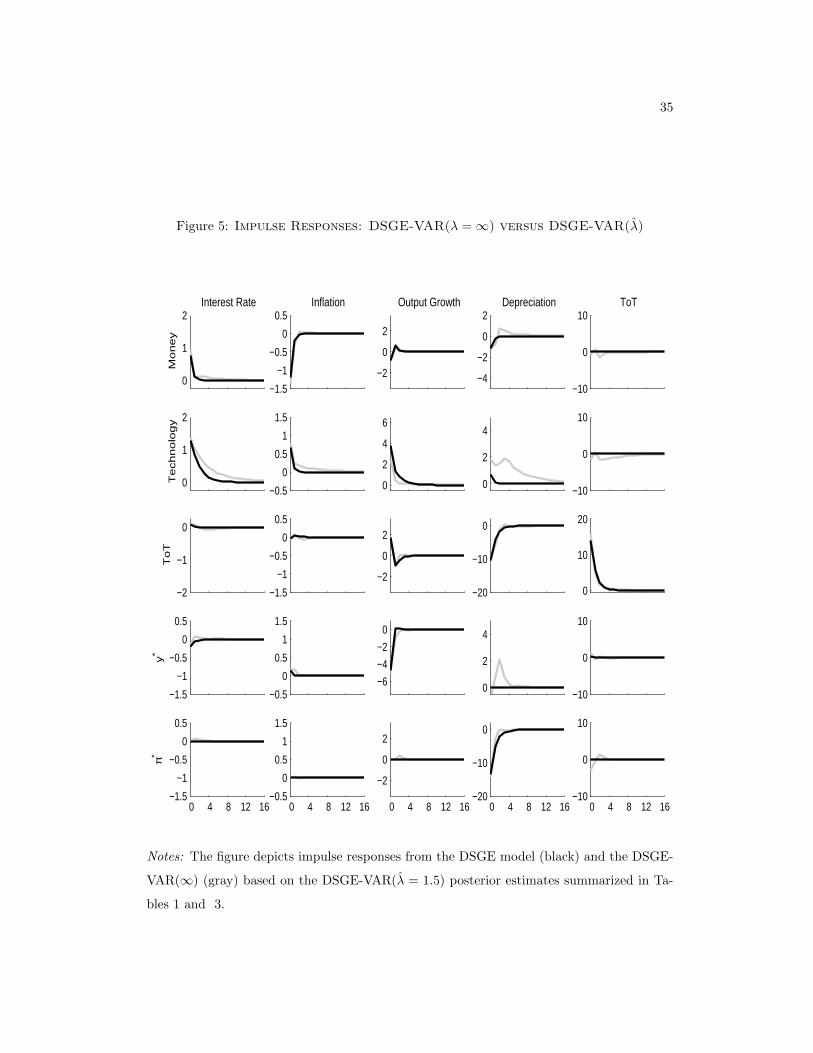
35

Figure 5: Impulse Responses: DSGE-VAR(λ = ∞) versus DSGE-VAR(λ)

0

1

2Interest Rate

Money

−1.5

−1

−0.5

0

0.5Inflation

−2

0

2

Output Growth

−4

−2

0

2Depreciation

−10

0

10ToT

0

1

2

Technolo

gy

−0.5

0

0.5

1

1.5

0

2

4

6

0

2

4

−10

0

10

−2

−1

0

ToT

−1.5

−1

−0.5

0

0.5

−2

0

2

−20

−10

0

0

10

20

−1.5

−1

−0.5

0

0.5

y*

−0.5

0

0.5

1

1.5

−6

−4

−2

0

0

2

4

−10

0

10

0 4 8 12 16−1.5

−1

−0.5

0

0.5

π*

0 4 8 12 16−0.5

0

0.5

1

1.5

0 4 8 12 16

−2

0

2

0 4 8 12 16−20

−10

0

0 4 8 12 16−10

0

10

Notes: The figure depicts impulse responses from the DSGE model (black) and the DSGE-

VAR(∞) (gray) based on the DSGE-VAR(λ = 1.5) posterior estimates summarized in Ta-

bles 1 and 3.

36

Figure 6: DSGE Model Impulse Responses as Function of ψ1

0

1

2Interest Rate

Money

−1.5

−1

−0.5

0

0.5Inflation

−2

0

2

Output Growth

−4

−2

0

2Depreciation

−10

0

10ToT

0

1

2

Technolo

gy

−0.5

0

0.5

1

1.5

0

2

4

6

0

2

4

−10

0

10

−2

−1

0

ToT

−1.5

−1

−0.5

0

0.5

−2

0

2

−20

−10

0

0

10

20

−1.5

−1

−0.5

0

0.5

y*

−0.5

0

0.5

1

1.5

−6

−4

−2

0

0

2

4

−10

0

10

0 4 8 12 16−1.5

−1

−0.5

0

0.5

π*

0 4 8 12 16−0.5

0

0.5

1

1.5

0 4 8 12 16

−2

0

2

0 4 8 12 16−20

−10

0

0 4 8 12 16−10

0

10

Notes: The figure plots the posterior mean of the DSGE model impulse responses computed

for three different values of the response to inflation in the policy rule, ψ1: 3.5 (black), 2.75

(dark gray), and 1.25 (light gray). The remaining policy parameters ψ2, ψ3, ψ4, and ρr are

kept at the baseline values of 0.125, 0, 0, and 0.5, respectively. For all impulse responses we

use the DSGE model posterior estimates of the non-policy parameters θ(np), summarized in

Table 3.

37

Figure 7: Comparative Performance of Policy Rules: Benchmark DSGE versus

DSGE-VAR(λ = 2) Parameter Estimates

1 1.5 2 2.5 3 3.5−2

0

2

4

6

8

10

12

14

ψ1

Notes: Posterior expected variance differentials as a function of ψ1 relative to baseline policy

rule ψ1 = 2.75. The remaining policy parameters ψ2, ψ3, ψ4, and ρr are kept at the baseline

values of 0.125, 0, 0, and 0.5, respectively. Negative differentials signify a variance reduction

relative to baseline rule. Differentials are computed using DSGE-VAR posterior (gray) and

DSGE model (black) posterior estimates of the non-policy parameters θ(np), summarized in

Table 3.

38

Figure 8: Comparative Performance of Policy Rules: DSGE versus DSGE-

VAR/Policy-Invariant Misspecification and DSGE-VAR/Backward-Looking

Analysis

1 1.5 2 2.5 3 3.5−2

0

2

4

6

8

10

12

14

ψ1

Notes: Posterior expected variance differentials as a function of ψ1 relative to baseline policy

rule ψ1 = 2.75. The remaining policy parameters ψ2, ψ3, ψ4, and ρr are kept at the baseline

values of 0.125, 0, 0, and 0.5, respectively. Negative differentials signify a variance reduc-

tion relative to baseline rule. Differentials are computed using the DSGE-VAR/Backward-

Looking Analysis (light gray), the DSGE-VAR/Policy-Invariant Misspecification scenario

(dark gray) and the DSGE model (black), where the latter uses the DSGE-VAR(λ = 2)

posterior estimates of the non-policy parameters θ(np), summarized in Table 3.

39

A Appendix: Model Derivation

Time t decisions are made after observing all current shocks. Variables with subscript t− s

where s ≥ 0 are known at time t. We assume that asset markets are complete. For each

state of nature there is a security that pays 1 Peso or 1 $.

A.1 Households

Domestic households solve the following decision problem

maxCht ,Nht ,Dht ,D∗

ht∞t=1

∞∑t=0

∑ht

βtP(ht|h0)

((Ct/Zt)1−σ − 1

1− σ− N1+ϕ

t

1 + ϕ

)(A.1)

s.t. PhtCht

+∑ht+1

(Qht+1|htDht+1 + Eht

Q∗ht+1|ht

D∗ht+1

)

≤WhtNht

+Dht+ Eht

D∗ht

+∫

Ωht(i)di,

where ht+τ denotes the history of events up to time t + τ , P(ht+τ |ht) its probability con-

ditional on time t information, Chtis consumption of a composite good in state ht, Nht

is

hours worked, Phtis the nominal price level of the composite good, Dht+τ

(D∗ht+τ

) is hold-

ings of a security that pays 1 unit of the domestic currency (foreign currency) in state ht+τ ,

Qht+τ |ht(Q∗

ht+τ |ht) its current price in Pesos (in state ht), Eht is the nominal exchange rate

(domestic currency/foreign currency), Thtare nominal transfers, and Ωht

(i) are (nominal)

dividends earned from domestic firm i. Note that∑

ht+1Qht+1|ht

= 1/Rhtis the inverse of

the one period gross nominal risk-free interest rate in Peso, and∑

ht+1Q∗

ht+1|ht= 1/R∗

htthe

inverse of the one-period gross nominal risk-free interest rate in $. Zt is a world technology

process, which is assumed to follow a random walk with drift. From now on we will use Xt

to denote a variable Xht, and IEt to denote

∑ht+τ

P(ht+τ |ht).

After detrending consumption and nominal wages according to ct = Ct/Zt and wt =

Wt/(PtZt), the first-order conditions can be written as

Nϕt = c−σ

t wt (A.2)

c−σt = βIEt[Rtc

−σt+1(zt+1πt+1)−1] (A.3)

0 = IEt

[(Rt −R∗

t et+1)c−σt+1

c−σt

(zt+1πt+1)−1

], (A.4)

where zt = Zt/Zt−1, πt = Pt/Pt−1 is the gross inflation rate, and et = Et/Et−1 is the gross

depreciation rate.

40

A.2 Terms of Trade and Real Exchange Rate

Let PH,t and PF,t be the domestic price of home and foreign produced goods, respectively.

Define the terms of trade:

Qt = PH,t/PF,t. (A.5)

We assume that the law of one price for foreign goods holds:

PF,t = EtP∗F,t, . (A.6)

Here P ∗F,t is the price of the foreign produced good in the foreign country, measured in

foreign currency. We also assume that domestically produced goods have a negligible weight

in foreign consumption. Specifically, let ϑ be the relative size of the domestic economy (to

be defined more precisely below). We define α∗ = ϑα and we let ϑ −→ 0. Hence, P ∗F,t will

be approximately equal to the foreign CPI P ∗t and we can express the terms of trade as

Qt = PH,t/(EtP∗t ). (A.7)

Both an exchange rate depreciation and foreign inflation reduce the terms of trade, i.e., make

imports more expensive. Let Pt be the domestic CPI. The real exchange rate is defined as:

St = EtP∗t /Pt. (A.8)

Thus, the relative price PH,t/Pt can be expressed as

PH,t/Pt = QtSt. (A.9)

A.3 Composite Goods

There are firms that buy quantities CH,t and CF,t of domestic and foreign produced goods

and package them into a composite good that is used for consumption by the households.

These firms maximize profits in a perfectly competitive environment:

maxCt,CH,t,CF,t

PtCt − PH,tCH,t − PF,tCF,t (A.10)

s.t. Ct =[(1− α)1/ηC

η−1η

H,t + α1/ηCη−1

η

F,t

] ηη−1

.

We deduce from the first-order conditions and a zero profit condition that

CH,t = (1− α)(PH,t

Pt

)−η

Ct, CF,t = α

(PF,t

Pt

)−η

Ct (A.11)

Pt =[(1− α)P 1−η

H,t + αP 1−ηF,t

] 11−η

. (A.12)

41

Dividing (A.12) by Pt and rearranging terms leads to the following relationship between the

real exchange rate and the terms of trade:

St =[(1− α)Q1−η

t + α] 1

η−1. (A.13)

The domestically produced good, supplied in overall quantity Yt, is itself a composite

made of a continuum of domestic intermediate goods Yt(i):

Yt =[∫ 1

0

Yt(i)ε−1

ε di

] εε−1

. (A.14)

We assume that there are perfectly competitive firms that buy the domestic intermediate

goods, package them, and resell the composite good to the firms that aggregate CH,t and

CF,t as well as abroad. These firms solve the following problem:

maxYt,Yt(i)

PH,tYt −∫ 1

0

PH,t(i)Yt(i)di (A.15)

s.t. Yt =[∫ 1

0

Yt(i)ε−1

ε di

] εε−1

.

The first order conditions and a zero-profit condition lead to

Yt(i) =(PH,t(i)PH,t

)−ε

Yt, PH,t =[∫ 1

0

PH,t(i)1−εdi

] 11−ε

. (A.16)

A.4 Domestic Intermediate Goods

The producers of the domestic intermediate goods Yt(i) are monopolistic competitors. Firms

can re-optimize prices in each period with probability 1 − θ. We assume that firms that

are unable to re-optimize their price, PH,t(i) will increase according to the steady state

inflation rate πH,∗. The firms use today’s prices of state-contingent securities to discount

future nominal profits. The firms’ production function is linear in labor:

Yt(i) = ZtNt(i), (A.17)

where productivity Zt is not firm specific and its growth rate zt = Zt/Zt−1 follows an AR(1)

process:

(ln zt − γ) = ρz(ln zt−1 − γ) + εzt , (A.18)

where γ is the steady state growth rate of productivity. The firms’ problem is given by:

maxPH,t(i), Yt+τ (i)∞τ=0

IEt

[ ∞∑τ=0

θτQt+τ |tYt+τ (i)(PH,t(i)πτ

H,∗ −MCnt+τ

)](A.19)

s.t. Yt+τ (i) ≤

(PH,t(i)πτ

H,∗

PH,t+τ

)−ε

Yt+τ ,

42

where MCnt+τ = Wt+τ/Zt+τ is the nominal marginal cost and Qt+τ |t is the time t price of

a security that pays 1 unit of domestic currency in period t+ τ .

We are considering a symmetric equilibrium in which all firms solve the same problem

and we eliminate the index i. The firms’ first-order condition can then be written as:

IEt

∞∑τ=0

θτQt+τ |t

(PH,tπ

τH,∗

PH,t+τ

)−ε

Yt+τ [(ε− 1)PH,tπτH,∗ − εMCn

t+τ ]

= 0. (A.20)

The fraction of firms that are allowed to re-optimize their price is 1 − θ, while all others

update their price by the steady state inflation rate. Hence

PH,t =[θP 1−ε

H,t + (1− θ)(πH,∗PH,t−1)1−ε] 1

1−ε

. (A.21)

We now express both the nominal marginal costs and the price chosen by firms that are

able re-optimize in terms of the price of the domestic good:

mct =MCn

t

PHt

=Wt

ZtPt

Pt

PHt

= wtQ−1t S−1

t and pH,t =PH,t

PH,t. (A.22)

Moreover, in equilibrium

Qt+τ |t = βτ λt+τ

λt= βτ c−σ

t+τPtZt

c−σt Pt+τZt+τ

. (A.23)

Thus, the optimal pricing rule can be re-stated as

pH,t =ε

ε− 1

IEt

[∑∞τ=0(βθ

τ )c−σ

t+τ

c−σt

(πτ

H,∗Qτs=1 πH,t+s

)−ε

St+τQt+τyt+τmct+τ

∏τs=1 πH,t+s

]IEt

[∑∞τ=0(βθτ )

c−σt+τ

c−σt

(πτ

H,∗Qτs=1 πH,t+s

)−ε

St+τQt+τyt+τπτH,∗

] .

(A.24)

Here we used the fact that PH,t/Pt = StQt. Moreover, we can re-write (A.21) as

1 =[θp1−ε

H,t + (1− θ)(πH,∗/πH,t−1)1−ε] 1

1−ε

. (A.25)

A.5 Domestic Market Clearing and Aggregate Production Func-

tion

The market for domestically produced goods clears if the following condition in terms of

variables detrended by Zt is satisfied

yt = cH,t + c∗H,t. (A.26)

43

After substituting (A.11) into (A.26) one obtains:

yt = cH,t + c∗H,t = (1− α)(PH,t

Pt

)−η

ct + αϑ

(PH,t/Et

P ∗t

)−η

c∗t

= (1− α) (StQt)−ηct + αϑQ−η

t c∗t . (A.27)

Finally, the aggregate production function for the domestic economy is given by

yt = Nt

[∫ (PH,t(i)PH,t

)−ε

di

]−1

. (A.28)

The households receive the profits generated by the monopolistically competitive do-

mestic intermediate goods producers. Firm i generates the following profit:

Ωt(i) = Yt(i)PH,t(i)−Nt(i)Wt.

Using the demand function (A.16) we can write

Ωt(i) = P 1−εH,t

Yt

P εH,t

−Nt(i)Wt.

Integrating both sides and using the expression for the price of the composite good, we

obtain ∫Ωt(i)di = PH,tYt −WtNt. (A.29)

Finally, we deduce from the budget constraint that

PhtCht

− PH,htYht

= Dht+ Eht

D∗ht−∑ht+1

(Qht+1|htDht+1 + Eht

Q∗ht+1|ht

D∗ht+1

). (A.30)

A.6 The Rest of the World

We begin by exploiting the perfect-risk-sharing assumption to obtain a relationship between

domestic and foreign consumption:(ct+1

ct

)σ

πt+1 =(c∗t+1

c∗t

)σ

π∗t+1et+1. (A.31)

Equation (A.31) can be rewritten as:(ct+1

c∗t+1

)σPt+1

Et+1P∗t+1

=(ctc∗t

)σPt

EtP∗t

.

This equation links consumption growth at home and abroad. To obtain implications about

the level of consumption in the two countries we assume that in period t = 0 S0 = 1.

Moreover, we let ϑ = C0/C∗0 . Hence, we deduce that in period t:

ct = ϑc∗tS1/σt . (A.32)

44

We can now rewrite the market clearing condition for the domestically produced good,

recalling that PH,t/Pt = QtSt. Substitute (A.32) into (A.27) and obtain:

yt = ϑc∗tQ−ηt

[(1− α)S1/σ−η

t + α]. (A.33)

In slight abuse of notation, the foreign analog of (A.30) is

EhtP ∗

htC∗

ht− Eht

P ∗F,ht

Y ∗ht

= DF,ht+ Eht

D∗F,ht

−∑ht+1

(Qht+1|htDF,ht+1 + EhtQ

∗ht+1|ht

D∗F,ht+1

).

Since all state-contingent securities are in zero net supply we obtain the following global

resource constraint from the budget constraints of the domestic and foreign households:

ct + Stc∗t = QtStyt + Sty

∗t . (A.34)

The equilibrium conditions are given by Equations (A.2), (A.3), (A.4), (A.8), (A.9),

(A.13), (A.22), (A.24), (A.25), (A.28), (A.32), (A.33). Moreover, we let ϑ −→ 0 and use

the approximation c∗t = y∗t . The system can be closed with interest rate feedback rules for

the domestic and foreign central banks.

A.7 Steady States

The central banks at home and abroad are determining the steady state inflation rates

π∗ and π∗∗ . Moreover, we assume that S0 = S∗ = 1. The consumption Euler equation

implies that the domestic nominal interest rate is R∗ = z∗π∗/β. A constant real interest

rate implies that the nominal exchange rate depreciation in steady state is e∗ = π∗/π∗∗ .

Uncovered interest rate parity determines the foreign nominal rate: R∗∗ = R∗/e∗. The terms

of trade are

Q∗ =[

11− α

(Sη−1∗ − α

)] 11−η

= 1.

Steady state inflation for the domestic good is πH,∗ = π∗. According to the small open

economy assumption c∗∗ = y∗∗ . Clearing of the domestic goods market requires y∗ = ϑy∗∗ .

Perfect risk sharing implies c∗ = ϑc∗∗. The supply side condition for the domestic good

determines the steady state labor input N∗ = y∗. Finally, we can determine y∗ from the

marginal cost condition

y∗ =(ε− 1ε

) 1ϕ+σ

.

Notice that now the global resource constraint (A.34) is indeed satisfied for Q∗ = 1.

45

A.8 Log-linearizations

We use the notation Xt to denote deviations of a variable Xt from its steady state X∗:

Xt = lnXt/X∗. The relationship between the real exchange rate and the terms of trade is

given by

St = −(1− α)Qt. (A.35)

Nominal exchange rates evolve according to

et = ∆St + πt − π∗t = −(1− α)qt + πt − π∗t , (A.36)

where qt = ∆Qt. Inflation in the relative price of the domestic good is given by

πH,t = πt + αqt. (A.37)

We can use the market clearing condition for the domestically produced good to determine

the level of the terms of trade

Qt = − 1η + (1− α)2(1/σ − η)

(yt − y∗t ). (A.38)

From perfect risk sharing and the market clearing condition for the foreign good we

have:

ct = c∗t + 1/σSt = y∗t − (1− α)/σQt

where we substituted for St using (A.35). We can now write the marginal costs as

mct = ϕyt + σy∗t +1

η + (1− α)2(1/σ − η)(yt − y∗t ) (A.39)

Define κ = (1 − θβ)(1 − θ)/θ. Marginal costs determine the inflation of the domestically

produced goods via the following Phillips curve:

πH,t = βIEt[πH,t+1] + κmct. (A.40)

The consumption Euler equation is of the form

ct = IEt[ct+1]−1σ

(Rt − IEt[πt+1 + zt+1]). (A.41)

Moreover, by combining the market clearing condition for the domestic good with the perfect

risk sharing condition, we deduce that

yt = ct − α(η + (1− α)(η − 1/σ))Qt. (A.42)

46

Equations (A.35) to (A.42) determine the evolution of Qt, St, et, πt, πH,t, mct, ct, and yt.

We treat π∗t and y∗t as exogenous and close the system with an interest rate feedback rule

that determines Rt.

In Section 2 of the main text we consider a version of the open economy model in which

ϕ = 0, η = 1, and 1/σ = τ . Notice that

η + (1− α)2(1/σ − η) = τ + α(2− α)(1− τ) = τ + λ,

where

λ = α(2− α)(1− τ).

We begin by determining the level of output yt in the absence of nominal rigidities, which

has to satisfy

0 = mct =1τy∗t +

1τ + λ

(yt − y∗t ).

We deduce that

yt = −λτy∗t .

The marginal costs satisfy

mct =1

τ + λ(yt − yt), (A.43)

which leads to the Phillips curve (5) reported in the main text:

πH,t = βIEt[πH,t+1] +κ

τ + λ(yt − yt). (A.44)

We will now manipulate the Euler equation. Using (A.42), replacing CPI inflation by

πH,t − α∆Qt, and plugging in (A.38) we can re-write the consumption Euler equation as

yt − yt = IEt[yt+1 − yt+1]− (τ + λ)(Rt − IEt[πH,t+1 + zt+1]), (A.45)

which is Equation (3) in the main text.

47

Figure A-1: VAR Approximation Error: DSGE vs DSGE-VAR(λ = ∞) Impulse

Responses

0

1

2Interest Rate

Money

−1.5

−1

−0.5

0

0.5Inflation

−2

0

2

Output Growth

−4

−2

0

2Depreciation

−10

0

10ToT

0

1

2

Technolo

gy

−0.5

0

0.5

1

1.5

0

2

4

6

0

2

4

−10

0

10

−2

−1

0

ToT

−1.5

−1

−0.5

0

0.5

−2

0

2

−20

−10

0

0

10

20

−1.5

−1

−0.5

0

0.5

y*

−0.5

0

0.5

1

1.5

−6

−4

−2

0

0

2

4

−10

0

10

0 4 8 12 16−1.5

−1

−0.5

0

0.5

π*

0 4 8 12 16−0.5

0

0.5

1

1.5

0 4 8 12 16

−2

0

2

0 4 8 12 16−20

−10

0

0 4 8 12 16−10

0

10

Notes: The figure depicts impulse responses from the DSGE model (black) and the DSGE-

VAR(∞) (gray) based on the DSGE-VAR(λ) posterior estimates summarized in Tables 1

and 3. The DSGE-VAR is estimated with two lags.