2

The authors wish to acknowledge financial assistance provided through Australian National Low Emissions Coal

Research and Development (ANLEC R&D). ANLEC R&D is supported by Australian Coal Association Low Emissions

Technology Limited and the Australian Government through the Clean Energy Initiative.

The authors also acknowledge Nick Hudson (CTSCo), Rob Heath (CTSCo) and Kevin Dodds (ANLEC) for their

exceptional support during the project. Thanks also to Rick Matthews, Nikki Accornero, and Paul Jensen.

Table of Contents 1 Executive Summary…………………………………………………………………………………………………………………………...…1

2 Introduction…………………………………………………………………………………………………………………………………….……2

3 Objectives and Approach……………………………………………………………………………………………………………….…....3

3.1 CTSCo’s Approach in the Context of Best Practice in Environmental Monitoring………...…3

3.1.1 Leakage Location…………………………….…………………………………………………...……….….4

3.1.2 Leakage Attribution……………………………………………………………………………………..……5

3.1.3 Leakage Quantification…………………………….……………………………………………………..…8

4 Process-based Approach for Signal Source Attribution……………………………..………………………….………………9

4.1 Relationship #1, O2 versus CO2………………………………………………………….……………………...……9

4.2 Relationship #2, CO2 versus N2………………………………………………………………………………..……10

4.3 Relationship #3 - CO2 versus N2/O2…………………………………………………………………………….…11

5 Materials and Methods………………………………………………………………………………………………………..………….…11

5.1 Field Methods…………………………………………………………………………………………..………….………11

5.1.1 Galvanic Cell Technology (O2) …………………………………………………….………….….……12

5.1.2 NDIR Technology (CO2 and CH4) …………………………………………………………….…..……13

5.1.3 Gas Chromatography (CO2, CH4, O2+Ar, N2) …………………………………………….…...…13

6 Data Assessment Methods…………………………………………………………………………………..……………………….……14

6.1 Standard GC data Reduction Method……………………………………………………….…………….……14

6.2 Sensor Data Reduction Method………………………………………………………………………..…………15

6.3 Data Quality Assessment……………………………………………………………………………………..………15

7 Results and Discussion……………………………………………………………………………………………………..……………..…16

7.1 Long-term Continuous Measurements………………………………………………..……….………………19

7.2 System and instrument sensitivity to Leakage……………………………………………….…….………21

7.3 Isotopes as an Attribution Tool…………………………………………………………………………………….25

8 Conclusions and Recommendations………………………………………………………………………………………….….…….27

9 References………………………………………………………………………………………………………………………………………….29

10 Appendices…………………………………………………………………………………………………………………………………….…33

Figures and Tables Figure 1. Flowchart of a process-based attribution method……………………………………………………………….……7

Figure 2. Stable carbon isotope signatures at CCS sites…………………………………………………………….…………..…8

Figure 3. Process-based relationship #1……………………..…………………………………………………………………….……10

Figure 4 Process-based relationship #2…………………………………………………………………………………………….……10

Figure 5. Process-based relationship #3………………………………………………………………………………………………...11

Figure 6. CTSCo's monitoring infrastructure………………………………………………………………………………………..…12

Figure 7. On-site GC analysis………………………………………………………………………………………………………………….14

Figure 8. Graphical description of the data comparison method used by Von Bobrutzki……………………....17

Figure 9. Statistical comparison of sensor versus GC data ………………………………………………..…………………..17

Figure 10. Sensor and GC data graphical interpretations…………………………………………………………….…………18

Figure 11. Data collected during the long-term tests…………………………………………………………..……….……….20

Figure 12. Process-based graphical representation of the long-term GC and sensor data sets……….….…21

Figure 13. Representation of volumes used in the leakage sensitivity modeling………………………….…….….22

Figure 14. Overall data trends for leakage input………………………………………………………………………………..….23

Figure 15. Magnified view of leakage input trends………………………………………………………………………………..24

Figure 16. Keeling isotope regression ........................................................................................................26

Figure 17. Isotope mixing model ……………………………………………………………………………………………………….….26

Table 1. Sensor technologies for continuous monitoring……………………………………………………………………… 12

Table 2. Average soil vapour concentrations measured at the site………………………………………………………..16

Table 3. Long-term test accuracies………………………………………………………………………………………………………..19

Table 4. Carbon and hydrogen isotope values………………………………………………………………………………….….. 25

Appendix 1. Point measurements analyzed by the GC at each monitoring site………………………………….… 33

Appendix 2. All soil vapour measurements (lab and field)…………………………………………………………………... 34

Appendix 3. Long term sensor and GC data for Site 2 SV01…………………………………………………………………. 35

Appendix 4. Long term sensor and GC data for Site 2 SV05…………………………………………………….........…… 36

1

1 Executive Summary

From February 24- March 7, 2017, Katherine Romanak travelled to Queensland Australia to provide

expertise and conduct research in environmental monitoring for the Carbon Transport and Storage

Corporation Pty Ltd (CTSCo) Surat CCS demonstration project. The project is designed to demonstrate

the technical viability, integration and safe operation of Carbon Capture and Storage (CCS) in the Surat

Basin. Currently in the feasibility study stage, the project is undergoing assessments and approvals in

environmental, social and technical aspects, under the relevant government regulation.

CTSCo’s overall approach to environmental M&V was found to be thorough and well-planned,

incorporating a variety of innovative and proven technologies for all of the major components of

environmental M&V: leakage location, attribution and quantification. A high priority is placed on the

well-being of the local community and the protection of the resources of local importance.

A gas chromatograph (gold standard approach) was used to characterize the dominant processes

occurring in the near-surface unsaturated zone and to test the performance of sensor installations to

perform process-based monitoring at the site. Process-based monitoring utilizes soil gas ratios to

indicate if CO2 is attributable to natural processes or CO2 leakage. The geochemistry of the near-surface

system was found to be simple with respiration as the main process and no detectable methane. The

system is therefore highly sensitive to indicating a leakage signal using a process-based monitoring

approach.

Sensor installations are well-constructed and robust, providing high quality real-time soil vapour data;

however there is an indication that sensors may lose accuracy over differing concentration ranges.

Carbon dioxide sensors appear to lose accuracy at higher concentrations, oxygen sensors may

potentially lose accuracy at lower concentrations, and there is an indication that methane sensors

overestimate concentrations. However, a sensitivity analysis of the system to leakage shows that sensor

inaccuracies are not large enough to significantly compromise the ability to detect leakage signal using

process-based geochemical relationships. The system is still extremely sensitive to leakage signals and

even with sensor error, leakage would be detected early and would be clearly identified.

The recommendation is to test the sensors in situ over varying gas concentration ranges to accurately

define sensor performance under fluctuating field conditions. This information is important for

understanding sensor performance over the long term when the environmental conditions may change.

Initial assessment of CO2 isotopic signature in the soil vapours and dissolved gases in underlying

groundwater suggests significant overlap among the various deep and shallow inputs. More assessment

of isotopic signatures, including characterization of 14C, is recommended.

2

2 Introduction

The Greenhouse Gas Storage Act 2009 (Queensland) was enacted to reduce the environmental impacts

of greenhouse gas (GHG) emissions by facilitating the storage of CO2 in subsurface geological formations

in the state of Queensland, Australia. This act provides for holders of GHG authorities to utilize

subsurface geological formations to store CO2 and to create a regulatory system to enable CO2 storage

activities. Under this Act, a monitoring and verification plan is required for observation and monitoring

any CO2 migration pathways that may occur before, during and after injection. In addition, the

Environmental Protection Act 1994 ensures the protection of Queensland’s environment during GHG

activities through implementation of effective environmental strategies with accountability for

environmental protection.

The Carbon Transport and Storage Corporation Pty Ltd (CTSCo) holds a Greenhouse Gas exploration

permit (EPQ7) issued by the Queensland Government under the Greenhouse Gas Storage Act 2009, to

demonstrate the technical viability, integration and safe operation of Carbon Capture and Storage (CCS)

in the Surat Basin. The project seeks to comply with the environmental requirements for Monitoring and

Verification (M&V) and lays the foundation for the development of best practice for future industrial

scale implementation of CCS in Australia onshore sedimentary basins.

In advance of CO2 storage, CTSCo is undergoing an Environmental Baseline Works (EBW) program at

their Glenhaven site, located 21 km SW of the town of Wandoan. The aim of the program is to

characterize the natural baseline conditions of the surface (atmosphere) and near-surface (shallow

groundwater of Surat Aquifers within the Springbok Sandstone and overlying unsaturated-zone soil

vapours). These shallow zones within the storage site are of great importance because; 1) they contain

the natural resources (groundwater and agricultural biosphere) that require the highest degree of

protection, 2) they are the regions of direct engagement between the project and local stakeholders,

and 3) they represent the surface boundary across which leakage to atmosphere is defined. Thus

accurately characterizing the natural baseline conditions lays the foundation for; 1) robust project

planning and development in predicting how a leakage signal might manifest in the near-surface, 2)

choosing the most useful parameters and strategies for identifying anomalous signals, and 3) attributing

the source of these signals as either being from CO2 storage activities or some other natural or

anthropogenic causes.

The main focus of the EBW is to implement a robust environmental M&V plan to support a fully-

integrated carbon capture and storage demonstration project planned for 2020. In addition, CTS l. c. is

seeking ways to balance robustness and cost-effectiveness to support industrial deployment of CCS. The

project proposes to make significant advances in method and instrument development towards

improving the following important components of near-surface M&V.

· Locating and anomaly that might signal leakage to atmosphere

· Correctly attributing the source of a detected anomaly

· Quickly and accurately responding to allegations of environmental harm

· Accurately delineating the areal extent of any leakage

3

· Predicting the fate of the CO2 within the environment

· Quantifying any CO2 lost from storage to atmosphere

· Monitoring to confirm that remediation efforts are effective

The University of Texas at Austin’s Bureau of Economic Geology (BEG) was contracted to assess the

quality of CTSCo’s environmental monitoring program and to recommend improvements, with a

particular focus on soil vapour monitoring. BEG’s experience includes developing and implementing

extensive near-surface monitoring, verification, and accounting programs at several United States

Department of Energy (US DOE) Regional Carbon Sequestration Partnership demonstration projects and

industrial sites (https://www.netl.doe.gov/research/coal/carbon-storage/carbon-storage-

infrastructure/rcsp). These sites include the Cranfield CO2-EOR site, where more than 2 million tonnes

of CO2 were stored over an 18-month period [1, 2], and the Hastings site, the geologic repository for

50,000 tonnes/year of CO2 captured from the world’s first fully-integrated CCS project on a coal-fired

power plant. Most recently, the BEG designed and implemented the environmental monitoring program

at West Ranch oilfield, the CO2 repository for the Petranova project, the world's largest post-combustion

carbon capture facility installed on an existing coal-fired power plant which recently began operation in

2016 (http://www.businesswire.com/news/home/20170109006496/en/). Here, more than 90 percent

of the CO2 from a 240 MW slipstream of flue gas is captured, yielding storage estimates of 1.6 million

tonnes/year at the West Ranch storage site. In 2011, the BEG was contracted by the International

Performance Assessment Centre for the Geologic Storage of Carbon Dioxide to (IPAC-CO2) to lead an

independent international team to assess the “Kerr leakage claim”. This was the first-ever claim of

leakage by a local landowner living above a geologic storage site; the Weyburn-Midale CO2 storage and

monitoring project in Saskatchewan Canada. This was a high-profile case where landowners publicly

claimed that CO2 from the CCS project was reaching ground surface and impacting their land [3]

(http://www.producer.com/2011/09/study-seeks-answers-to-farms-hydrocarbon-puzzle/). The project

was the first to attribute the source of an anomaly and the first to address a leakage claim which

required a prompt, cost effective and accurate response, and much was learned from the experience.

The claim was later disproven by three different research groups of which the BEG was the only

“independent” group lacking previous ties to the CO2 storage project. Thus BEG has extensive experience

in environmental monitoring with which to assess and inform activities at the CTSCo project site.

3 Objectives and Approach

The objective of this study is to assess the degree to which CTSCo’s environmental monitoring activities

are robust, including the approach, quality of monitoring installations and data collection systems with a

focus on soil vapour monitoring in the vadose zone. Such an assessment includes characterization of the

geochemical signatures in the near-surface at Glenhaven to indicate the sensitivity of the system to

leakage identification. The assessment also defines any potential interferences or challenges that should

be addressed and makes suggestions on how monitoring can be improved for ease of implementation

and cost-effectiveness without sacrificing accuracy. The project also has the goal of upscaling proven

technologies for industrial applications by implementing real-time continuous monitoring capabilities.

https://www.netl.doe.gov/research/coal/carbon-storage/carbon-storage-infrastructure/rcsp

https://www.netl.doe.gov/research/coal/carbon-storage/carbon-storage-infrastructure/rcsp

http://www.businesswire.com/news/home/20170109006496/en/

http://www.producer.com/2011/09/study-seeks-answers-to-farms-hydrocarbon-puzzle/

4

Thus an additional objective of BEG’s assessment is to ensure that these technological advancements

are performing with an accuracy and sensitivity adequate for the environmental M&V program.

Our approach was to conduct a short field campaign to collect data at the site using gas

chromatography. Gas chromatography is the current “gold standard” technology for implementing the

specific soil vapour monitoring approaches that will be applied at Glenhaven. These data were then used

to determine the accuracy and precision of the sensor installations that are providing real-time

continuous monitoring at the site. Field validation and performance assessment of the two

measurement techniques were accomplished by; 1) comparing the precision and accuracy of the two

measurement types as a function of environmental variability and 2) assessing the validity of an

amended data reduction protocol which is necessary when using sensors in place of a GC.

3.1 CTSCo’s Approach in the Context of Best Practice in Environmental

Monitoring

Here we discuss how CTSCo’s plan for near-surface monitoring aligns with current best practices for

environmental monitoring at geologic CO2 storage sites. Whereas we will briefly comment on CTSCo’s

overall approach, our main focus is on soil vapour monitoring applied in the vadose zone, with an

emphasis on source attribution.

Best practice for near-surface leakage assessment generally includes three main components which can

be applied in one or a combination of any of the surface/near surface environments (e.g. groundwater,

vadose zone, atmosphere): 1) detection or location of an anomaly that might represent leakage, 2)

source attribution of the anomaly, and 3) quantification monitoring of emissions from leakage [4]. Thus

an anomalous occurrence of CO2 must first be detected or located, then it must be attributed either to

leakage from the storage formation or some other source not related to CO2 storage. Then, if attributed

to leakage, leakage must be quantified. In all cases “trigger points” or criteria that determine when

additional or heightened next steps are warranted are critical to the decision-making process.

3.1.1 Leakage Location

A range of approaches and technologies can be used within the large monitoring areas associated with

geologic CO2 carbon storage sites to detect anomalies that might indicate CO2 leakage. First, routine

wide-area monitoring efforts can seek to cover wide areas using airborne or ground-based open-path

infrared or laser-based approaches [5] [6] [7] [8], or remote geochemical surveys [9] [7] [10, 11].

Biological monitoring methods [12, 13] can be used for delineating environmental change which may

signal leakage. Second, risk assessment can be used to inform and direct targeted monitoring to the

most likely areas of CO2 migration (e.g. near faults, fractures, or wellbores) [14] [15]. Risk assessment is

especially useful in areas where remote large-area monitoring is more challenging for example due to

interferences from thick vegetation and topography. Third, and perhaps one of the most important

ways in which leakage may be indicated is via local stakeholders living near geological storage sites.

Similar to the Kerr leakage claim, [3] landowners and local stakeholders may report what they perceive

as environmental impacts caused by leakage from the CO2 storage formation. In this case, protocols for

5

responding to concerns must be in place before a project begins and clearly defined with methods that

can attribute whether the environmental change is natural or results from subsurface activities either

related to CO2 storage or other industries that may be active in the area.

CTSCo’s plan for leakage location is robust in that it incorporates a well-thought mixture of the three

main approaches; wide-area monitoring, risk assessment, and stakeholder engagement as follows:

1. CTSCo is conducting a risk assessment following Glencore’s methodology which is based on

international standards for risk assessment. The approach incorporates a risk and consequence

matrix which will be used to target monitoring to higher-risk areas.

2. For wide-area monitoring, a combination of eddy covariance, remote hyperspectral imaging and

atmospheric tomography are being deployed. Eddy covariance is a low-cost and established

monitoring technique that can provide automated continuous measurement of CO2 surface

fluxes over a wide area for potential leakage location. The technique can be used in relatively

inaccessible areas and should be well-suited to the low topography and relatively unobstructed

terrain of the area [16-18]. Atmospheric tomography is similar in that it involves using several

sensors that measure atmospheric CO2 concentrations and a device to measure wind speed and

direction to determine the CO2 source location and size [19-21]. Remote spectral imaging will be

used to monitor ecosystem health with a particular focus on the health of buffel grass (Cenchrus

ciliaris), a ranchland grazing resource important to local stakeholders. Spectral imaging is a well-

established technique for accurately measuring the health of vegetation by detecting changes in

spectral reflectance due to changes in chlorophyll content and this technique has been

demonstrated in CO2 storage applications [12, 22, 23].

3. CTSCo’s monitoring approach focuses on protecting resources of local importance and

incorporates a high degree of engagement with the local community. This approach represents

a high value placed on stakeholder protection and values, and the open communication being

established between project and the community should ensure that any public leakage claim

will be easily communicated and quickly addressed.

Thus it is BEG’s assessment that CTSCo is currently planning a comprehensive and robust program for

locating leakage that surpasses most project designs. The combination of these approaches will provide

a thorough areal coverage for demonstrating storage permanence with respect to the biosphere. It

should be noted that the experience gained in using these methods may lead to a prioritization of

technologies. Not all methods deployed at the demonstration will necessarily be used at future sites.

Also, the research component of the project will provide technological advancement that will play into

future decisions regarding monitoring plan design. In these ways, the work being done by CTSCo is

important for finding an optimized balance between cost-effectiveness and robustness for upscaling CCS

technology.

3.1.2 Leakage Attribution

Leakage attribution is the main focus of BEG’s involvement. Once an anomaly that may indicate leakage

is detected, attribution must be quick and accurate. This is a critically important step yet it can be a

6

difficult task. Whereas vadose zone soil vapour methodologies are perhaps the most convenient

methods for assessment due to the inexpensive cost and ease of access to the vadose zone, soil vapour

CO2 concentrations are highly variable in space and time and affected by transient environmental

conditions and potential industrial interferences. Thus a challenge in this area has always been how to

identify a leakage signal in the presence of natural variations.

In the near surface environment at Glenhaven, production of natural CO2 and CH4 from in-situ biological

activity in both the unsaturated zone and shallow groundwater aquifers may input to the soil vapour

signal. Potential natural in-situ vadose zone processes may include 1) biologic respiration, 2) CO2

dissolution, 3) CH4 production, 4) transformation (oxidation) of CH4 into CO2, and 5) mixing between

atmosphere and soil vapour. Agricultural and ranching practices may also have an impact, but perhaps

of greatest importance is the potential for interferences from nearby coal seam gas (CSG) production.

Activities to recover hydrocarbon gases from the Walloon Coal Measures could release methane in the

project area, or methane from underlying coal may migrate into the near-surface from natural seepage

over geologic time. Additionally, methane may migrate through abandoned wells or wellbores that have

lost well bore integrity. Because CH4 readily transforms or “oxidizes” to CO2 in the vadose zone, CH4

could indirectly produce a secondary false leakage signal. If natural accumulations of CO2 exist within

the basin stratigraphy, these gases may also rise to the surface over geologic time mimicking the effects

of a CO2 storage release.

Many regulations (e.g. IPCC Greenhouse Gas Guidelines, EU CCS Directive, UNFCCC Clean Development

Mechanism, and US EPA Class VI and Subpart RR) require comparison of pre-injection baseline CO2

concentrations with post-injection concentrations for leakage attribution [4]. The purpose of such

monitoring is to define local, natural pre-injection CO2 distributions over space and time. In theory, with

“normal” CO2 concentrations defined, any statistically significant increases in CO2 during a storage

project would indicate leakage from the project. Whereas an increase in CO2 concentrations can signal

an anomalous change that may suggest leakage, this method will not be adequate to attribute the

source of the change. First, it has recently been understood that soil respiration rates, which are

responsible for most of the natural CO2 production in soils, are increasing due to climate change, itself

[24]. Thus we now understand that “baseline” CO2 concentrations will be moving targets over time.

Second, as we learned from the Kerr leakage claim, soil CO2 baselines cannot be measured everywhere

within the large storage project area. If concerns arise in an area lacking local baseline measurements,

the degree to which available measurements (from nearby locations) are representative as baseline may

be called into question. Soil vapour in areas without direct baseline data may be vulnerable to

misinterpretation and, if not properly assessed, could be mistaken for a leakage signal. Assuming

straight-away that any CO2 increase over baseline indicates leakage, will likely lead to a high occurrence

of false positives which may fuel unnecessary public concern and project delays.

Furthermore, methods relying on comparing pre- and post-injection CO2 soil vapour concentrations for

discriminating leakage are cumbersome and time-consuming because they require large and complex

spatial and temporal data sets. Whereas these data provide useful information, they should not be

solely relied upon for attribution. Such a methodology is challenged as an “industrial appropriate”

technique due to such complexity. In theory, pre-injection soil vapour measurements and supporting

7

weather data (rainfall, temperature, and barometric pressure) must be collected from between 1-3

years pre-injection [25] and assessed using complex statistical analysis to aid in understanding and ruling

out environmental variability as the cause of the anomaly. Defining clear trigger points using this

method is difficult and has not yet been documented in an actual in practice. Such a methodology does

not show promise for providing quick and accurate response to public concerns about environmental

impacts.

A development of the standard is the quicker, cheaper “process-based” method. Thus to enhance the

accuracy of using baseline measurements for attribution, CTSCo is implementing a process-based

monitoring technique [4, 26, 27] of which the BEG has been instrumental in developing. The technique

has gained endorsement as “an important development … and a powerful baseline-independent

method” as stated in a recent publication on the state of art in monitoring and verification 10 years on

[28] from the 2005 IPCC Special Report on Carbon Dioxide Capture and Storage [29]. In addition to the

BEG sites of Cranfield, Hastings, and West Ranch, and at the Kerr Farm, the method has been

implemented at a number of other project sites including the Otway project in Australia [30],the

Aquistore Project in Canada (Cameron McNaughton, personal communication), CO2Field Lab in Norway

[5], the U.S. Department of Energy Bell Creek demonstration site in Montana, USA (John Hamling,

personal communication), and at a CO2-rich artesian well failure analog at Qinghai, China [31]. Leading

Japanese scientists are now adapting the method for use in offshore environments [32].

Rather than solely relying on complex comparisons of CO2 concentrations pre- and post- injection, the

process-based method uses the geochemical relationships among simple gases (CO2, N2, O2, and CH4) to

describe natural soil processes. These relationships, which will be discussed in greater detail below,

account for naturally-occurring subsurface, biogeochemical processes that can add or deplete CO2 in the

vadose zone – hence the moniker “process-based”. Using this approach, potential leakage signals can

be identified instantaneously using

graphical representation of three

geochemical relationships. Trigger points

are clearly, simply, and universally defined.

CO2 concentrations exceeding the values

shown to be natural from a process-based

analysis are attributed to exogenous

sources such as CO2 leakage from the deep

storage formation and require further

assessment, and in this way, anomalies can

be quickly screened. Using such a method,

near-surface MVA is much simpler, and

more accurate and economical for large-

scale deployment of CCS, and make

evidence of storage permanence more Figure 1. Flowchart showing the components of a process-based attribution method. CTSCo is working on optimizing methods for determining the origin of an exogenous gas signature.

8

accessible to stakeholders and the general public because of its graphical nature and simplicity.

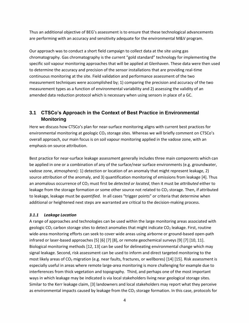
The flow chart in Figure 1 shows that a process-

based approach will indicate if a gas has been

naturally generated in situ or if it has an

exogenous origin. If generated in situ, no

additional action is needed. If the gas is

attributed to an exogenous source, more

assessment is required to link the anomaly to

either CCS or other non-CCS-related activities.

Carbon isotopes are thought to be an important

method for providing information on the origin

of CO2 and CH4 in soil vapour and the processes

that gave rise to their formation [33-37],

however, there can be strong limitations with

this method. We have observed considerable

overlap between the carbon isotopic signatures

(δ13C) of some anthropogenic CO2 emissions

that will be stored at geologic sites with

background sources [7, 38, 39] (Figure 2). Such isotopic overlap was responsible for the confusion at the

Kerr Farm where leakage was initially concluded based on the δ13C signature of the CO2 ‘anomaly’ which

matched that of the CO2 injected at the site [3]. Thus, confusion over carbon isotopes was a leading

factor in incorrect attribution. CTSCo and BEG hope to collaborate on an in-depth research project to

characterize the potential isotopic signals at Glenhaven to define how isotopes may contribute to a

robust attribution method. Preliminary results on isotopes are reported herein.

The only current drawback to process-based monitoring is a lack of measurement technology to

implement the methodology with real-time, continuous data collection. For most gases of interest,

currently-available sensors can provide continuous monitoring since they are compact, fully automated,

can be dedicated to a site, have data transmission capabilities, and do not require consumable supplies.

However, not all of the sensors needed for a process-based analysis are commercially-available.

Whereas compact cost-effective commercially-available sensors exist for some of the gases important to

a process-based analysis (O2, CO2, and CH4), none exist for field-based N2 measurement. One of the

research-related activities of the CTSCo Glenhaven project is to develop accurate real-time process-

based measurement technology. A process-based approach to addressing monitoring requirements,

together with advances in continuous real-time measurement capabilities will provide M&V that meets

the intent of the regulations with high confidence and low cost compared to alternate approaches.

3.1.3 Leakage Quantification

If leakage is unequivocally attributed, regulations require quantification of emissions. Quantification will

occur at or just above ground surface, the interface across which leakage to atmosphere is defined.

Figure 2. Stable carbon isotope signatures of various potential leakage and background signals at CCS sites.

9

Approaches and technologies that detect CO2 over large areas, such as eddy covariance and atmospheric

tomography, are also relevant for quantification; however, these methods will also require some type of

attribution technology to ensure that quantification only includes actual leakage emissions and not

natural baseline emissions. Quantification will require delineating the areal extent of leakage (apart

from natural signals), predicting the fate of the CO2 within the environment (e.g. what amount, if any,

will be naturally attenuated and how), and confirming if and to what degree remediation efforts are

effective. A process-based analysis is effective for quantification in that it can apportion naturally-

produced CO2 from CO2 contributed by leakage. If this apportionment can be correlated with surface

flux measurements, a definitive leakage quantification can be made. Thus the combination of CTSCo’s

wide area monitoring efforts with eddy covariance and atmospheric tomography, in addition to process-

based soil vapour analysis will provide a state-of the art foundation for emissions quantification and

remediation monitoring in the rare event that it is needed.

4 Process-based Approach for Signal Source Attribution

CTSCo’s vadose-zone monitoring plan incorporates process-based analysis as a primary technique, and

we will now give a general description of the technical aspects of this method to preface our

assessment.

Beginning with the composition of the natural atmosphere (78% N2, 21% O2, 0.04% CO2), carbon cycling

processes in the unsaturated zone will alter the geochemistry of soil vapour in predictable ways that can

be used to identify the processes involved [40], [41], [42]. When these processes are understood, the

dominant sources of soil vapours can be determined even in the absence of prolonged baseline data or

when naturally occurring in-situ and exogenous gases are mixed. If the observed CO2 concentration

exceeds the level that would be expected from the coexisting O2 concentration, then excess CO2 may be

attributed to leakage. Note that the absolute CO2 concentration is not significant; rather it is the

relationship of the CO2 to coexisting gases that is of importance. This is because the gas proportions of

vadose zone biogeochemical processes are preserved in the gas ratios. If the ratios indicate natural

processes, there is no leakage. If the ratios indicate addition of exogenous gas into the system, leakage

is possible and requires further assessment [43]. The level of certainty is increased by examination of

several different relationships in sequence which we will now explain further.

4.1 Relationship #1, CO2 versus O2

Air is constantly and naturally pumped in and out of soils by changes in barometric pressure. During low

barometric pressure fronts, vapours are drawn upward out of permeable soils and into the atmosphere.

Conversely, during high barometric pressure fronts, air is pushed downward into the soil. Diurnal and

seasonal air temperature fluctuations, surface wind speeds and evaporation also play a role. Thus, if no

biologic processes were active in soils, soil vapour concentrations would be those of air. According to

equation 1 below, biologic respiration in the soil will consume 1 mole (or 1 volume %) of soil O2 and

produce 1 mole (or volume %) of soil CO2 according to the reaction:

10

CH2O (organic matter) + O2 → CO2 + H2O (1)

Alternatively, when respiration rate outpaces that of O2

influx, such as in wet or waterlogged soils, O2 can

become severely depleted. When this occurs,

anaerobic bacteria produce CH4. When CH4 migrates

into oxygenated zones, or when environmental change

results in an influx of O2 into a previously oxygen-

devoid environment, CH4 is oxidized to CO2. This

process consumes 2 moles (or volume %) of O2 and

produces 1 mole (or volume %) CO2 according to the

following equation:

CH4 + 2O2 → CO2 + 2H2O (2)

These common natural processes result in predictable

deviations from atmospheric concentrations for CO2

and O2 along a trend with a slope of -1 for biologic

respiration and -0.5 for methane oxidation (Figure 3).

CO2 concentrations less than those predicted from O2 concentrations based on these relationships signal

either a mixture of gases undergoing multiple processes or most commonly a loss of CO2 via gas

dissolution into recharging groundwater. Alternatively, addition of CO2, such as might be released from a

CO2 storage formation will create CO2 concentrations larger than would be expected from corresponding

O2 concentrations. Thus in this graphical representation, vapour concentrations plotting on or to the left

of the line represent natural processes and concentrations to the right of the respiration line indicate

potential leakage signal. The main benefit to this criteria is that the respiration line represents a clear

and universal trigger threshold that is immediately understood by both experts and laymen.

4.2 Relationship #2, CO2 versus N2

Further knowledge of soil processes can be gained by

studying the relationship of N2 with CO2 (Figure 4).

Because gas concentrations are measured in percent

(by volume or molar), any non-reactive addition or

subtraction of a gas component will, by definition,

dilute or concentrate (respectively) all other gas

components. N2, a relatively non-reactive but major

component in air and soil vapour can be used as a

sort of “tracer” to indicate this process. Used in

conjunction with the relationships between CO2 and

O2 described above, CO2 that shows a negative

correlation with N2 signals dilution by input of

exogenous gas [41, 44] and CO2 that shows a positive

Figure 3. Process-based relationship showing the trends for respiration, methane oxidation, CO2 dissolution and leakage signal. Concentrations that lie to the left of the line indicate natural processes and concentrations that lie to the right of the line indicate potential leakage.

Figure 4. This process-based relationship gives a clear representation of whether a gas is being added from outside the system (exogenous), or whether a gas is lost through a process such as dissolution (natural).

11

correlation with N2 indicates dissolution of CO2. [40, 42]. This same relationship using CH4 versus N2 can

be used to indicate exogenous methane input into the system in the case of leakage from CSG

operations.

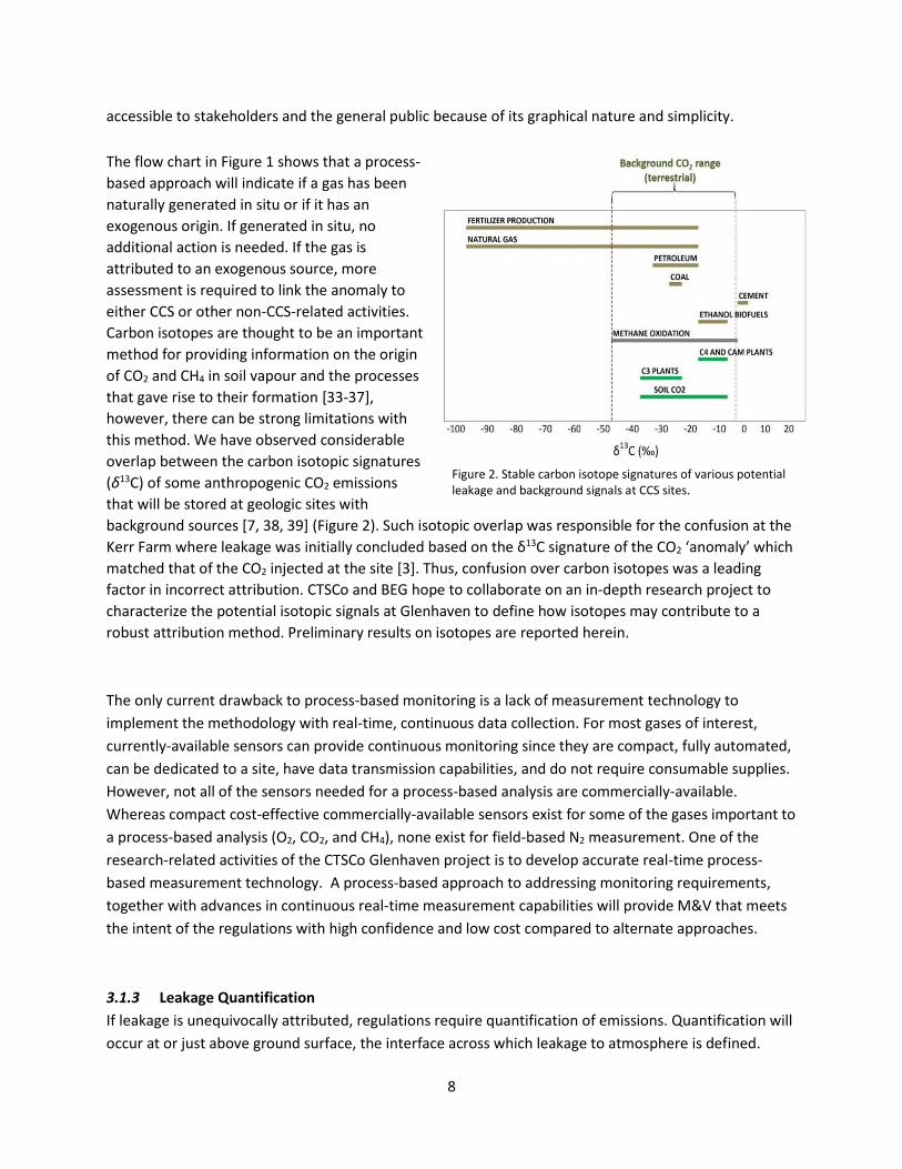
4.3 Relationship #3 - CO2 versus N2/O2

This relationship (Figure 5) indicates the degree to

which O2 is being utilized in the system. This

information is useful for understanding the magnitude

of methane oxidation. N2 is generally non-reactive, but

O2 is utilized in respiration, and to a larger degree in

CH4 oxidation. Air continuously invades the soil

supplying both N2 and O2 in a ratio of 3.4. When O2 is

utilized in biologic reactions, this ratio increases above

the atmospheric ratio of 3.4. In more complex systems,

especially where CH4 is abundant and vigorously

oxidized to CO2, the ratio of N2/O2 can reach several

orders of magnitude higher than 3.4 [42]. This effect is

especially enhanced when CH4 is not produced in-situ

but is exogenous, coming from depth at a high flux rate.

Thus this relationship, when used with the information provided from the relationships described above,

adds to the understanding of the processes acting in the system and on CO2 concentrations.

5 Materials and Methods

5.1 Field Methods

CTSCo’s near-surface EBW program comprises 5 monitoring sites within the monitoring area, one of

which measures weather parameters, and four which each contain 4 monitoring stations. The

monitoring stations include soil vapor monitoring wells at 1-meter (SV01) and 5-meter (SV05) depths

and groundwater wells at 10-meter (GW10) and 20 meter- (GW20) depths (Figure 6). Each soil vapour

installation contains a dedicated down-hole sensor cluster comprised of commercially-available sensors

for monitoring process-based gases (CO2, O2, CH4) (Table 1) either in the soils or in the head-space above

ground water. Commercially-available sensors do not currently exist for N2. Real-time data are acquired

and transferred by 3G-ftp to a cloud database (PI historian). Spot readings are also taken on-site during

site visits when sensors can be pulled out of the well and calibrated if needed.

Figure 5. This relationship illustrates the magnitude to which O2 is utilized due to respiration or methane oxidation.

12

5.1.1 Galvanic Cell Technology (O2)

Electrochemical (galvanic) sensors that measure O2 operate using a sensing electrode (cathode) and a

counter electrode (anode) separated by electrolyte. A hydrophobic membrane enables gas diffusion and

reaction with the sensor electrode, producing an electrical signal proportional to the concentration of

the gas. Electrochemical sensors generally have linear output with good selectivity, repeatability, and

accuracy. Cross sensitivity is not a concern. Instead, the greatest potential challenge to data quality is

degradation of sensor components. Extremely dry or humid environments can affect the water content

of the electrolyte solution and destabilize the sensor. Also, any condensation on the membrane will

inhibit gas diffusion into the cell and degrade response time and accuracy [45].

Figure 6. (Left) One of CTSCo's monitoring stations comprising two soil vapor wells and two groundwater wells. (Right) A sensor cluster has been pulled out of the well for maintenance. Instruments are deployed downhole within a packer system and provide real-time data acquisition.

Table 1. Sensor technologies used for continuous real-time measurement of geochemical components.

13

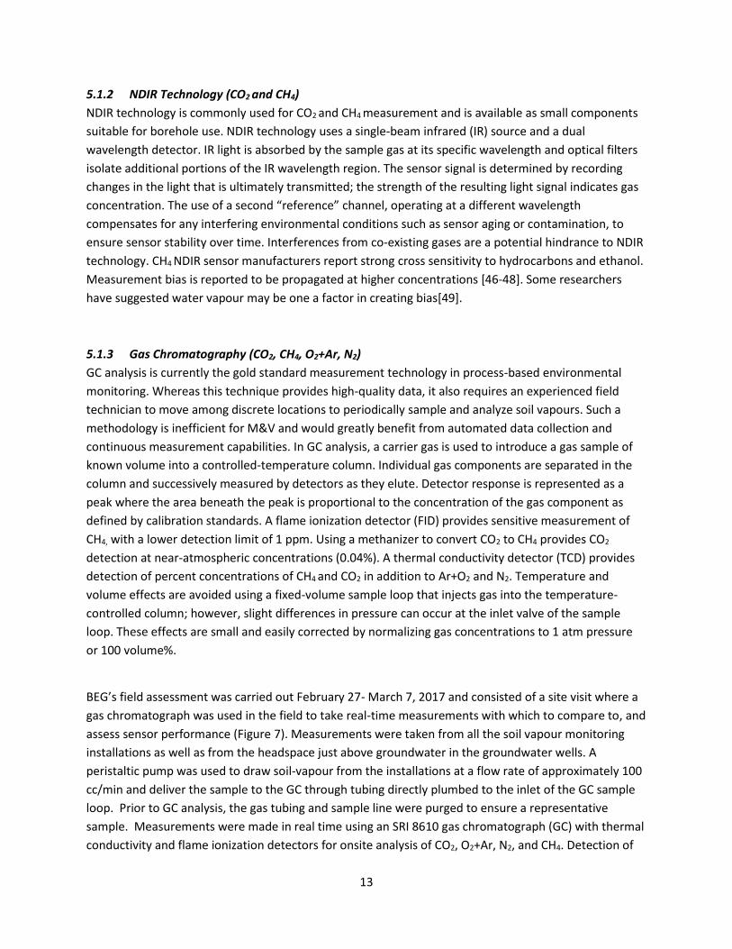
5.1.2 NDIR Technology (CO2 and CH4)

NDIR technology is commonly used for CO2 and CH4 measurement and is available as small components

suitable for borehole use. NDIR technology uses a single-beam infrared (IR) source and a dual

wavelength detector. IR light is absorbed by the sample gas at its specific wavelength and optical filters

isolate additional portions of the IR wavelength region. The sensor signal is determined by recording

changes in the light that is ultimately transmitted; the strength of the resulting light signal indicates gas

concentration. The use of a second “reference” channel, operating at a different wavelength

compensates for any interfering environmental conditions such as sensor aging or contamination, to

ensure sensor stability over time. Interferences from co-existing gases are a potential hindrance to NDIR

technology. CH4 NDIR sensor manufacturers report strong cross sensitivity to hydrocarbons and ethanol.

Measurement bias is reported to be propagated at higher concentrations [46-48]. Some researchers

have suggested water vapour may be one a factor in creating bias[49].

5.1.3 Gas Chromatography (CO2, CH4, O2+Ar, N2)

GC analysis is currently the gold standard measurement technology in process-based environmental

monitoring. Whereas this technique provides high-quality data, it also requires an experienced field

technician to move among discrete locations to periodically sample and analyze soil vapours. Such a

methodology is inefficient for M&V and would greatly benefit from automated data collection and

continuous measurement capabilities. In GC analysis, a carrier gas is used to introduce a gas sample of

known volume into a controlled-temperature column. Individual gas components are separated in the

column and successively measured by detectors as they elute. Detector response is represented as a

peak where the area beneath the peak is proportional to the concentration of the gas component as

defined by calibration standards. A flame ionization detector (FID) provides sensitive measurement of

CH4, with a lower detection limit of 1 ppm. Using a methanizer to convert CO2 to CH4 provides CO2

detection at near-atmospheric concentrations (0.04%). A thermal conductivity detector (TCD) provides

detection of percent concentrations of CH4 and CO2 in addition to Ar+O2 and N2. Temperature and

volume effects are avoided using a fixed-volume sample loop that injects gas into the temperature-

controlled column; however, slight differences in pressure can occur at the inlet valve of the sample

loop. These effects are small and easily corrected by normalizing gas concentrations to 1 atm pressure

or 100 volume%.

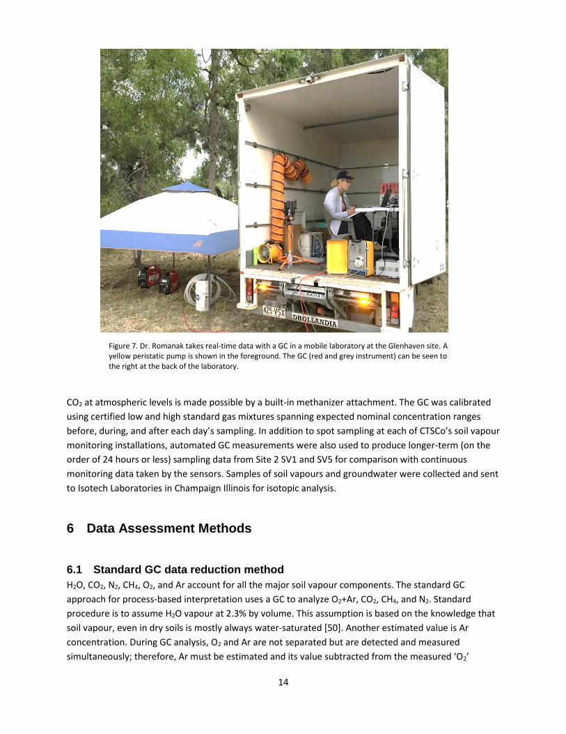
BEG’s field assessment was carried out February 27- March 7, 2017 and consisted of a site visit where a

gas chromatograph was used in the field to take real-time measurements with which to compare to, and

assess sensor performance (Figure 7). Measurements were taken from all the soil vapour monitoring

installations as well as from the headspace just above groundwater in the groundwater wells. A

peristaltic pump was used to draw soil-vapour from the installations at a flow rate of approximately 100

cc/min and deliver the sample to the GC through tubing directly plumbed to the inlet of the GC sample

loop. Prior to GC analysis, the gas tubing and sample line were purged to ensure a representative

sample. Measurements were made in real time using an SRI 8610 gas chromatograph (GC) with thermal

conductivity and flame ionization detectors for onsite analysis of CO2, O2+Ar, N2, and CH4. Detection of

14

CO2 at atmospheric levels is made possible by a built-in methanizer attachment. The GC was calibrated

using certified low and high standard gas mixtures spanning expected nominal concentration ranges

before, during, and after each day’s sampling. In addition to spot sampling at each of CTSCo’s soil vapour

monitoring installations, automated GC measurements were also used to produce longer-term (on the

order of 24 hours or less) sampling data from Site 2 SV1 and SV5 for comparison with continuous

monitoring data taken by the sensors. Samples of soil vapours and groundwater were collected and sent

to Isotech Laboratories in Champaign Illinois for isotopic analysis.

6 Data Assessment Methods

6.1 Standard GC data reduction method

H2O, CO2, N2, CH4, O2, and Ar account for all the major soil vapour components. The standard GC

approach for process-based interpretation uses a GC to analyze O2+Ar, CO2, CH4, and N2. Standard

procedure is to assume H2O vapour at 2.3% by volume. This assumption is based on the knowledge that

soil vapour, even in dry soils is mostly always water-saturated [50]. Another estimated value is Ar

concentration. During GC analysis, O2 and Ar are not separated but are detected and measured

simultaneously; therefore, Ar must be estimated and its value subtracted from the measured ‘O2’

Figure 7. Dr. Romanak takes real-time data with a GC in a mobile laboratory at the Glenhaven site. A yellow peristatic pump is shown in the foreground. The GC (red and grey instrument) can be seen to the right at the back of the laboratory.

15

concentration. Due to the overall non-reactivity of both Ar and N2 in most soils, the Ar/N2 ratio can be

assumed to be or 1/83 which is the ratio of the components found in the atmosphere. This assumption

holds true except in rare cases of extreme denitrification in sediments [51]. Using this approach, Ar is

therefore estimated as 1/83 the N2 concentration and subtracted from the O2 measurement. Finally,

when all components have been either measured or estimated, gas concentrations are then normalized

to 100 volume % [52]. In all instances, when more than one measurement was taken at a single location,

the average of those measurements are reported.

6.2 Sensor Data Reduction Method

Because the sensors do not analyze for N2, which is an important component of the process-based

analysis, N2 must be estimated by difference. With the concentrations of most major soil vapors (CO2,

O2, and CH4) measured by sensors, the difference between 100% and the total of these concentrations

will be equal to N2+H20+ Ar. For our analysis we allot 2.3% to H2O, 0.9% to Ar, and the rest of the

difference we allot as N2. Future data assessment can seek to utilize relative humidity (RH)

measurements to determine the accuracy of using 2.3% water vapor content.

6.3 Data Quality Assessment

In order to best compare the data quality of a method that utilizes sensors to a method that utilizes a

GC, it is necessary to evaluate the uncertainty of each measurement type. A simple sensitivity analysis

was performed to quantify and assesses the error in sensor measurement relative to GC. The main

components of our analysis are accuracy (defined as the agreement of a measured value with its true

value), and precision (defined as the degree of closeness in independent measurements made under the

same conditions). For the purposes of this study, we define the “measured value” as the sensor data and

the “true value” as the GC data. We also consider the two data collection methods to be independent

measurements made under the same conditions; thus both accuracy and precision are represented as

absolute error (also termed absolute uncertainty) and reported as the difference (denoted as ∆) in gas

concentrations measured by each of the methods. In some instances we ignore the absolute notation to

show the direction of the inaccuracy. For example, we calculate the ∆ in gas concentrations as GC data -

Sensor data and we report the numerical sign to indicate whether the sensor measurement was higher

or lower than the GC, as this discussion becomes relevant to our assessment.

The accuracy of GC measurements is widely known to be 2% of each measurement (e.g relative

uncertainty). Assuming O2 concentrations as high as 21%, the acceptable relative uncertainty of this

measurement is 0.4%. Assuming CO2 which can be as high as 18% in natural environments [42, 53], the

relative uncertainty of this measurement is also about 0.4%. Rounding these uncertainties up to 0.5%,

and assuming the rest of the measured vapour components (Ar, CH4, and H2O) are negligible, the

combined uncorrelated uncertainty for N2 is 0.7%. Thus the difference (denoted as ∆) in gas

concentrations between the GC and sensors should not exceed 0.5 for CO2 and O2 measured by sensors

16

and 0.7 for N2 calculated by difference in order for the sensors to meet the same standards as are

provided by using gas chromatography.

7 Results and Discussion

We compare data sets from two types of sample collection methods; point measurements and long-

term measurements. We also compare two methods of data analysis and reduction techniques: those

that measure N2 and those that calculate N2 by difference. This comparison of measurement techniques

is necessary because of the lack of currently available continuous monitoring sensor capabilities for N2.

In essence, the data reduction method for sensors, if accurate, could suffice for the lack of real-time N2

data supplied by sensors.

Average data concentrations measured during the BEG field visit are reported in Table 2. GC point

measurements at all the monitoring sites ranged from 0.04% to 3.17% CO2 and from 18.35% to 20.71%

O2. CH4 was not detected by the GC. N2 measured by the GC ranged from 74.98% to 77.46%. Sensor

measurements ranged from non-detectable to 2.60% for CO2, and 18.80% to 20.90% for O2. The in-situ

sensors yielded a maximum reading of 0.33% for CH4 in soil vapours. This reading was unsubstantiated

by GC measurements, none of which showed measurable CH4 to be present in soil vapours at the site

except for traces found in the headspace above deep (20-meter) groundwater above the Walloon coal

measures. N2 calculated by difference using the sensor data ranged from 75.48% to 76.4%.

A comparison of the error in each sensor measurement to the defined relative uncertainty of the

corresponding GC measurement shows that 91% of CO2 measurements and 73% of the O2

measurements are within the acceptable accuracy range of a GC. 73% of the calculated N2 values fit the

requirement for 0.7% absolute accuracy.

To further assess the agreement between sensor and GC measurements, data were compared and

statistically evaluated according to the method employed by Von Bobrutzki et al. [54]. This method is used

to compare the accuracy of data measured by the sensors to that of the GC. As shown in Figure 8, perfect

agreement between GC and sensor measurements would yield a regression through the origin with a

Table 2. Average soil vapour concentrations measured at the site. Sensor measurements are compared to the GC data for accuracy and precision. Highlighted values are out of the range of our defined acceptable accuracy range.

17

slope of 1. If sensor error propagates systematically as a function of concentration, two potential linear

trends could result. If error overestimates values at high concentrations, Δ values (GC-Sensor) will be

negative and regressions will indicate positive y-intercepts (left). Conversely when sensor error

underestimates values, Δ values will be positive and regressions will have negative y-intercepts (right).

Regressions (Figure 9) on data collected at the Glenhaven site show that CO2 sensor data are highly

correlated with GC measurements at the concentrations measured at the site, with a slope of 1.24, a y-

intercept near 0 (-0.051) and a high R2 of 0.979. The regression hints at a slight but potentially systematic

linear error where the CO2 sensor underestimate concentrations at high concentrations. In any case, CO2

sensor measurements performed very well, with 91% of the measurements falling within the defined

acceptable accuracy.

Statistical analysis of O2 measurements indicate slightly less accuracy than CO2 measurements, having a

y-intercept for the regression of 3.9 and an R2 of 0.55. Note that the y-intercept for O2 data regression is

highly positive, whereas the y-intercept for CO2 data is a slightly negative value. This difference in the

regressions suggest that, in contrast to CO2 sensors may potentially underestimate values at high

concentrations, O2 sensors may potentially overestimate values at high O2 concentrations.

Figure 9. Statistical comparison of sensor versus GC data.

Figure 8. Graphical description of the data comparison method used by Von Bobrutzki.

18

The accuracy of N2 calculated by difference using sensor O2 and CO2 data are compared to N2

concentrations directly measured with the GC. The comparison shows low accuracy with a y-intercept of

71.66 and an R2 of near zero. However such a comparison for N2 may be less relevant because N2

concentrations do not significantly deviate in natural environments. As previously discussed, N2 acts as a

conservative tracer and its concentration does not change during the natural processes of respiration or

methane oxidation or mixing with air. Therefore this regression represents scatter within the data rather

than a trend over a range of concentrations. Despite the apparent lack of correlation, N2 data calculated

by difference have the same accuracy as O2 measurements with 71% of the data falling within the

acceptable defined limits.

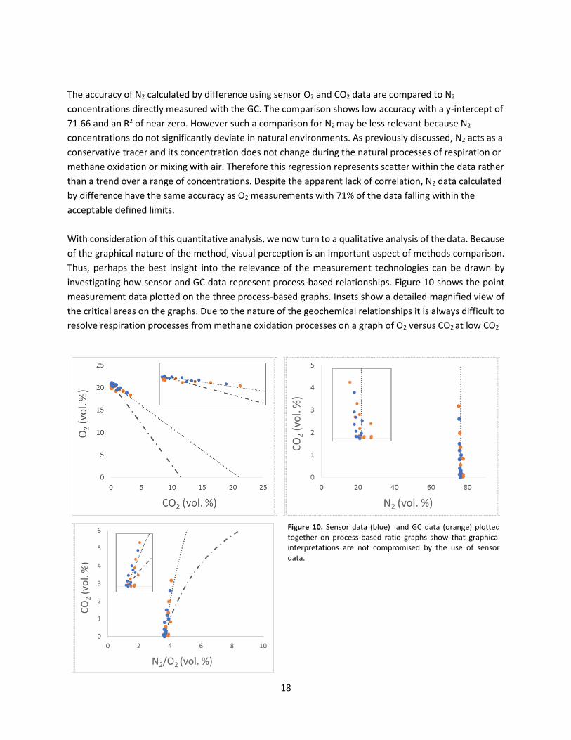
With consideration of this quantitative analysis, we now turn to a qualitative analysis of the data. Because

of the graphical nature of the method, visual perception is an important aspect of methods comparison.

Thus, perhaps the best insight into the relevance of the measurement technologies can be drawn by

investigating how sensor and GC data represent process-based relationships. Figure 10 shows the point

measurement data plotted on the three process-based graphs. Insets show a detailed magnified view of

the critical areas on the graphs. Due to the nature of the geochemical relationships it is always difficult to

resolve respiration processes from methane oxidation processes on a graph of O2 versus CO2 at low CO2

Figure 10. Sensor data (blue) and GC data (orange) plotted together on process-based ratio graphs show that graphical interpretations are not compromised by the use of sensor data.

19

concentrations: however at CO2 concentrations above about 2% the respiration and methane oxidation

trends begin to deviate, making the distinction clearer. At these concentrations, the respiration trend is

clearly discernable with both sensor and GC data indicating respiration. Thus the same conclusions about

the system would be drawn from either data measurement technique. Despite some data scatter, the

same conclusions are drawn upon inspection of the remaining concentration relationships, indicating that

the sensor data are accurately displaying the correct relationships required for attribution using a process-

based method.

7.1 Long-term continuous measurements

The main advantage of data collection using sensors is the continuous real-time data measurement

capabilities. Two longer-term experiments were performed to compare continuous data acquisition of

sensors and the GC. The GC was deployed in automated mode to take measurements every 15 minutes

to compare to the sensor’s continuous data collection at Site 2, both within the 1-meter and 5-meter

depths. The test at SV01 occurred from March 3 at 18:36 to March 4 13:06 (18.5 hours) and the test at

SV05 occurred from March 4 at 14:15 to March 5 at 7:15 (17 hours). During the tests, soil vapours were

continuously pumped at a slow rate of about 80 mls/minute from the borehole into the GC. Because

most sensors are designed for installation in heating and air conditioning ducts, sensors should tolerate

flow rates of many liters per minute. Long-term GC measurements at Site 2 SV01 ranged from 0.89% to

1.19% for CO2, 19.86% to 20.17% for O2, and 75.81% to 76.02% for N2. Sensor readings ranged from

1.14% to 1.27% for CO2, 18.95% to 19.12% for O2, and 76.52% to 76.75% for N2 as calculate by

difference. Long term GC measurements at Site 2 SV05 ranged from 2.55% to 2.72% for CO2, 17.49% to

17.65% for O2, and 76.44% to 76.64% for N2 and sensor readings ranged from 1.14% to 1.27% for CO2,

18.95% to 19.12% for O2, and from 76.60% and 76.73% for N2 as calculated by difference.

A graph of soil vapour concentrations measured by both the GC and sensors over time in both wells is

shown in Figure 11 and calculated accuracies for the long term test measurements are shown in Table 3.

Although not perfectly correlated, the data from both methods show relatively similar concentration

variations over time. Perhaps the most meaningful observation is that the CO2 sensor is in very good

agreement with the GC at SV01 where CO2 is relatively low (about 1 %). At this site, 100% of sensor

accuracies and precisions are in acceptable ranges (Table 3). However, at SV05, where CO2

concentrations are significantly higher (about 2.5 %), the CO2 sensor critically underestimates CO2

concentrations. None of the

accuracies are within acceptable

ranges and their Δ values are >

1. This trend is consistent with

the results shown in Figure 9. Statistical comparison of sensor versus

GC data. which suggests that the

CO2 sensor may underestimate

values at higher CO2

concentrations.

Table 3. Calculated accuracies for the long term tests at SV01 (36 measurements) and SV05 (33 measurements).

20

The O2 sensor data do not conform to the assumption that O2 sensors will overestimate concentrations at higher O2 values. Instead, the O2 sensor reads slightly lower than the GC at SV01 where O2 is relatively high (about 20 %) and yields positive Δ values that average ~ 1 %. However at SV05 where the O2 concentration is slightly lower (about 18 %) the sensor does overestimate the values with an average Δ value of -0.74. It is interesting to note that if sensor technologies are found to systematically underestimate CO2 and overestimate O2, these imprecisions may counterbalance each other to yield relatively accurate N2 concentrations by difference. Thus even when individual CO2 and O2 measurements are imprecise, they may yield precise and accurate N2 values. Such an effect is clearly seen at SV05 where none of the sensor CO2 or O2 readings fall within the desired accuracy, however all of the N2 by differences are highly accurate and precise. This is not the case at SV01 where all of the CO2

Figure 11. Sensor data (shown in blue) and GC data (shown in orange) collected during the long-term tests.

21

sensor readings are acceptable, none of the O2 readings are acceptable, and only 19% of the N2 by difference are achieve the desired accuracy and precision.

7.2 System and instrument sensitivity to leakage

Baseline soil vapour values indicate respiration is the main process at Glenhaven. In the absence of

complex processes, the system is theoretically simple and highly sensitive to a leakage signal. As

previously stated, grab samples yielded good relationships between the GC and the sensors despite an

indication of some bias at certain concentration levels. We now compare the long-term continuous GC

and sensor data in Figure 12 with the understanding that continuous pumping may create a

measurement artifact in the sensor data. Sensor data collected at SV01 do not appear to significantly

compromise the ability to identify a leakage signal, however the sensor data at SV05 do appear as

Figure 12. Process-based graphical representation of the long-term GC and sensor data sets.

SV01 SV05

22

though they might compromise the ability to interpret leakage at the site. To quantitatively assess and

understand the consequences of this degree of sensor inaccuracy, average soil vapour concentrations

for each well depth were calculated from the long-term data and a hypothetical leak of CO2 was

modelled into each representative gas mixture until the soil vapour approached 100% CO2. For purely

illustration purposes, if we take a random representative volume of 3 liters of soil with a porosity of 0.3,

we assume a constant gas-filled pore volume of 1 liter at normal temperature and pressure (NTP) of

20⁰C and 1 atm. We then add CO2 in increments of 0.446 mmoles to reach a total of 100% CO2 or a total

of 44.6 mmoles CO2. To put this amount of CO2 into an understandable perspective, each increment of

leakage amounts to about 9 ml of pure CO2 invading 1000 mls of gas-filled pore space within a 3-liter

package of soil with 30% porosity. These relative volumes are represented in Figure 13 to attempt to

show the relatively small volume of CO2 that is incrementally added to the system in the model. Given

that 1 tonne of CO2 contains 22.7 x 106

mmoles of CO2 and occupies a volume of 556

liters at NTP, each increment of modeled CO2

accounts for a tiny fraction of a tonne of CO2.

The total amount added is on the order of

1/50,000 or 0.002% leakage of a tonne of

CO2.

Figure 14 shows the overall leakage trends

for each process-based graph at both soil

vapor wells and Figure 15 shows the detailed

trends with modelled leakage increments. To

understand the degree to which sensor

inaccuracies could be detrimental to

identifying a leakage signal, we assess the

amount of

CO2 required to push the soil vapor concentrations into the leakage fields on process-based graphs and

compare the differences between the sensor and GC data. Each of the first five data points on each

leakage trend represents the addition of 9 mls of CO2 gas leakage into the liter of pore space. We

assume the sensors retain their initial degree of accuracy as CO2 increases. First, it is apparent that

regardless of the initial condition as defined by the sensors, the two leakage scenarios eventually

converge towards 100% CO2. Thus with our assumptions in place, over time the two measurements will

converge. Looking at Figure 15, there is no difference between sensor and GC data in the amount of CO2

gas input that would be recognized as leakage in process-based relationship #1 at SV1 or in process-

based relationship 2 at SV05. Both assessments would lead to leakage recognition within the first

modelled increment of CO2 input. For relationship 2 at SV01 and relationships 1 and 3 at SV05, only 1

additional increment of leakage would be required for the sensors to indicate leakage (9 mls more than

with sensors). Only process-based relationship 2 at SV1 would require significantly more CO2 input

(45mls) for sensors to register a leakage signal, and even this amount is tiny when compared to the 1000

mls of gas-filled pore space. (45mls) for sensors to register a leakage signal, and even this amount is tiny

when compared to the 1000 mls of gas-filled pore space.

Figure 13. Representation of volumes used in modelling leakage sensitivity.

23

Figure 14. Modelled leakage trends indicated by a grey arrow, show how gas concentrations in the near-surface system at Glenhaven would react to leakage input. A more detailed assessment is presented in Figure 15.

Leakage trend

Leakage trend

Respiration line Respiration line

Res

pir

atio

n li

ne

Res

pir

atio

n li

ne

24

Figure 15. Magnified view of incremental modelled leakage input at SV01 and SV05. Despite a slight lack of accuracy for sensor data, the system is very sensitive to leakage whether using sensors or a GC to implement a process-based approach.

25

7.3 Isotopes as an Attribution Tool

As previously discussed there are a number potential inputs to the soil vapour signal at Glenhaven. A

thorough assessment of these inputs will be critical for understanding if and how isotopes might be used

as a leakage attribution tool in the event that data from process-based monitoring exceeds a trigger

point, indicating a potential CO2 leakage from the storage project. Some of the most relevant of these

may be to compare the oxidation products of CH4 from Walloon coal, flue gas from the Millmerran

power station, and natural soil respiration values. Another indicator with perhaps the most promising

potential is radiogenic carbon (14C). A recent advance comparing the stable carbon isotopic ratio of CO2

(δ 13C) with its radiogenic carbon (14C) signature was used at the Kerr Farm [55] and shows promise for

attribution. A value of 14C near 100 percent modern carbon (pMC) indicates young CO2 produced by

plants and microbes in the near-surface. Values of 14C close to 0 pMC are significantly older and

represent carbon from deeper ancient geologic formations, including from coal and natural gas, and are

likely to represent leakage. By adding 14C to an isotopic assessment, attribution of a gas anomaly may be

more accurately achieved. BEG and CTSCo hope to investigate the potential for these isotopic methods

at Glenhaven.

To carry out a preliminary assessment of isotopic signals at Glenhaven, soil vapors from the unsaturated

zone and dissolved gases in groundwater were collected from the four monitoring stations during the

BEG field campaign. These samples were analyzed for carbon isotopes of CO2 (δ13CO2) and CH4 (δ13CH4)

and hydrogen (deuterium) isotopes of CH4 (δDCH4). Data are shown in Table 4.

Of the 15 soil vapor samples submitted for analysis, 8 samples yielded CO2 concentrations high enough

(>0.60 %) to determine δ13CO2 values. These data ranged from -11.38 ‰ to -18.09 ‰. None of the soil

vapour samples contained CH4.

Table 4. Carbon and hydrogen isotope values for gases and dissolved gases at Glenhaven. All data are reported in ‰. The designation of “LT” refers to samples collected during the long term test.

Soil vapour samples δ13CO2

GH-0317-2-SV5 -18.09

GH-0317-2-SV5-LT -17.98

GH-0317-2-SVI -16.46

GH-0317-2-SVI-LT -17.11

GH-0317-3-SV5 -16.33

GH-0317-3-SVI -11.38

GH-0317-4-SV5 -15.54

GH-0317-5-SVI -14.87Dissolved gases in

groundwater δ13CO2 δ13CH4 δDCH4

GH-0317-2-GW10 -21.55

GH-0317-5-GW10 -22.08

GH-0317-2-GW20 -23.39 -63.35 -219.4

GH-0317-4-GW20 -29.38

GH-0317-3-GW20 -26.62 -74.94 -218.6

GH-0317-5-GW20 -24.33 -75.31 -223.3

26

Of the 6 groundwater samples submitted for dissolved gas analysis, all of the samples contained

sufficient CO2 and three of the samples contained sufficient CH4 (> 1%) for isotopic analysis. All of the

groundwater samples with sufficient CH4 for isotopic analysis were from GW20 wells which are

completed in Surat Basin formations above the Walloon Coal Measures. Isotopic data were not assessed

for this report.

The CO2 isotopic data were analyzed in two stages.

First, a Keeling plot [56, 57] was constructed with

the soil vapour isotope values (Figure 16). This type

of plot is standard for assessing the overall isotopic

value of respired CO2 in a system with multiple

respiration inputs that vary over space and time

and mix with air. With the exception of one outlier

sample (-17.11), the data are well-correlated. The y-

intercept points to an overall respiration value of -

18.97. This value was then used to represent the

isotopic signature of natural CO2 respiration at

Glenhaven within our mixing models (Figure 17)

The mixing model provides a preliminary view of a 3-component mixing system that includes CO2 from

soil respiration, air, and dissolved gases in groundwater that might migrate into the vadose zone. Our

first assessment investigated if simple mixing between the Keeling respiration value and air (CO2 = -7.2

‰) could account for the variation in soil vapor data. This model is represented in figure 17 as a black

-35

-30

-25

-20

-15

-10

-5

0

0 5 10 15 20 25 30 35 40

δ13

CO

2 (‰

)

CO2 (volume %)

Soil vapour

GW 20

GW10

Keeling value mixed with air

Keeling value mixed with 3-SV01

Air

Figure 17. Mixing model using carbon isotopic signatures of air, soil vapors and dissolved gases in underlying groundwater at the Glenhaven site.

Figure 16. A Keeling regression indicates the carbon isotope signature of the Glenhaven soil vapour system.

27

dotted line. This scenario could not account for the variation in samples because the resultant δ13CO2 are

significantly more negative than the measured soil vapour samples. Next, CO2 from Springbok

groundwater wells (GW20) and shallow intervals in the Springbok alluvial groundwater (GW10), and the

respiration value supplied by the Keeling plot were mixed with the least negative of the soil vapor

samples (- 11.38 at 3-SV-01). The data envelope defined by these curves were relatively consistent with

the data, however significant input into the vadose zone from gases dissolved in underlying

groundwater would show an exogenous signal on process-based ratio plots. Thus it appears that there

may be significant isotopic overlap among the various potential inputs at the site. More in-depth

assessment is needed.

8 Conclusions and Recommendations

The BEG visited the Glenhaven field site from February 24- March 7, 2017 to provide an initial site

characterization and assessment of CTSCo’s environmental M&V. BEG has designed and implemented

environmental monitoring programs at several demonstration and industrial geologic CO2 storage sites

and found CTSCo’s overall approach to be well-balanced and robust, surpassing many other project

designs currently in operation worldwide. CTSCo’s approach includes a wide array of the most

innovative proven technologies for location and attribution of potential leakage signals. These

technologies can also be applied to quantification if needed. CTSCo is also commended for placing a high

importance on stakeholder priorities and for their efforts in establishing open and transparent

communication with the local community.

CTSCo is implementing a process-based soil vapour monitoring methodology of which the BEG has been

involved in developing. The method has been used successfully at several CCS sites worldwide and in

several different CCS applications, however a main drawback to the method is a lack of continuous

monitoring capabilities for effective use at industrial scale. CTSCo is researching whether currently

existing sensor technologies could provide the needed measurement capabilities. Thus a main focus of

BEGs visit was to provide an initial characterization of the geochemical signatures at the site and to test

the quality of monitoring installations and data collection systems. A preliminary assessment of the

isotopes signatures was also undertaken.

The results of the field test are as follows:

The vadose zone geochemistry at Glenhaven is simple and straightforward with respiration as

the dominant process. Methane is virtually absent from the vadose zone.

CO2 sensors are accurate and precise at low CO2 concentrations (~1%), but there is indication

that accuracy may be lost at higher concentrations (~2.5%). O2 sensors hint at a similar but

opposite effect in data quality. Thus even when CO2 and O2 are not precise or accurate, N2

calculated by difference can be fortuitously precise and accurate. Future investigations should

seek to understand the degree to which continuous pumping may affect sensor accuracy.

Methane sensors appeared to overestimate the methane in the system but have not been

thoroughly tested due to the lack of methane in the Glenhaven near-surface.

28

The apparent lack of sensor performance under certain conditions does not compromise the

ability to indicate leakage using process-based ratios. The system is still extremely sensitive to

leakage signals and even with sensor error, leakage would be detected early and would be

clearly identified.

Initial assessment of CO2 isotopic signature in the soil vapours and dissolved gases in underlying

formations suggests overlap among the various deep and shallow inputs.

In summary, the approach and monitoring installations at Glenhaven are sufficiently robust and

adequate for leakage detection, however more investigation is needed to understand how sensors will

perform at different concentration ranges. It is recommended that the sensors be subjected in situ to

higher CO2 and CH4 concentrations, perhaps with small controlled releases within the boreholes. Such a

test would indicate the sensors response and performance under changing conditions. Isotopic

signatures also warrant further and more intricate analysis and should include an assessment of 14C as a

potential tracer of leakage.

29

9 References [1] S.D. Hovorka, T.A. Meckel, R.H. Trevino, Monitoring a large-volume injection at Cranfield, Mississippi—Project design and recommendations, International Journal of Greenhouse Gas Control, (2013) 345-360. [2] C. Yang, K. Romanak, S.D. Hovorka, R.M. Holt, J. Lindner, R. Trevino, Near-surface monitoring of large-volume CO2 injection at Cranfield: Early field test of SECARB phase III, SPE Journal, 18 (2013) 486-494. [3] P. Lafleur, Geochemical Soil Gas Survey: A Site Investigation of SW30-5-13-W2M, Weyburn Field, Saskatchewan, Monitoring Project Number 2. Saskatoon, SK, in, Petro-Find Geochem Ltd., 2011. [4] T. Dixon, K.D. Romanak, Improving monitoring protocols for CO2 geological storage with technical advances in CO2 attribution monitoring, International Journal of Greenhouse Gas Control, 41 (2015) 29-40. [5] D.G. Jones, Monitoring of near surface gas seepage from a shallow injection experiment at the CO2 Field Lab, Norway, International Journal of Greenhouse Gas Control, 28 (2014) 300-317. [6] L. Spangler, L. Dobeck, K. Repasky, A. Nehrir, S. Humphries, J. Barr, C. Keith, J. Shaw, J. Rouse, A. Cunningham, S. Benson, C. Oldenburg, J. Lewicki, A. Wells, Diehl, B. Strazisar, J. Fessenden, T. Rahn, J. Amonette, J. Barr, W. Pickles, J. Jacobson, E. Silver, E. Male, H. Rauch, K. Gullickson, R. Trautz, Y. Kharaka, J. Birkholzer, L. Wielopolski, A shallow subsurface controlled release facility in Bozeman, Montana, USA, for testing near surface CO2 detection techniques and transport models, Environmental Earth Sciences, 60 (2010) 227-239. [7] R. Govindan, A. Korre, S. Durucan, C.E. Imrie, A geostatistical and probabilistic spectral image processing methodology for monitoring potential CO 2 leakages on the surface, International Journal of Greenhouse Gas Control, 5 (2011) 589-597. [8] J. Dobler, T. Zaccheo, N. Blume, M. Braun, C. Botos, T.G. Pernini, Spatial mapping of greenhouse gases using laser absorption spectrometers at local scales of interest, in: SPIE Remote Sensing, International Society for Optics and Photonics, 2015, pp. 96450K-96450K-96413. [9] P. Shuler, Y. Tang, Atmospheric CO2 monitoring systems, Carbon Dioxide Capture for Storage in Deep Geologic Formations—Results from the CO2 Capture Project, v. 2: Geologic Storage of Carbon Dioxide with Monitoring and Verification, SM Benson, in, Elsevier Science, London, 2005. [10] J.C. Pashin, P.E. Clark, M.R. McIntyre-Redden, R.E. Carroll, R.A. Esposito, A.Y. Oudinot, G.J. Koperna, SECARB CO 2 injection test in mature coalbed methane reservoirs of the Black Warrior Basin, Blue Creek Field, Alabama, International Journal of Coal Geology, 144 (2015) 71-87. [11] A. Marchese, T. Vaughn, D. Zimmerle, D. Martinez, L. Williams, A. Robinson, A. Mitchell, R. Subramanian, D. Tkacik, J. Roscioli, S. Herndon, Methane Emissions from United States Natural Gas Gathering and Processing, Environ. Sci. Technol., (2015). [12] E.J. Male, W.L. Pickles, E.A. Silver, G.D. Hoffmann, J. Lewicki, M. Apple, K. Repasky, E.A. Burton, Using hyperspectral plant signatures for CO2 leak detection during the 2008 ZERT CO2 sequestration field experiment in Bozeman, Montana, Environmental Earth Sciences, 60 (2010) 251-261. [13] R.R. Noble, L. Stalker, S.A. Wakelin, B. Pejcic, M.I. Leybourne, A.L. Hortle, K. Michael, Biological monitoring for carbon capture and storage–A review and potential future developments, International Journal of Greenhouse Gas Control, 10 (2012) 520-535. [14] M. Buric, K. Chen, J. Falk, S. Woodruff, Enhanced spontaneous Raman scattering and gas composition analysis using a photonic crystal fiber, Applied Optics, 47 (2008) 4255. [15] R. Chen, P. Codella, R. Guida, A. Zribi, A. Vert, R. Potyrailo, M. Baller, Photonic bandgap fiber-enabled Raman detection of nitrogen gas, in: Defense, Security, and Sensing, SPIE, 2009, pp. 73220N.

30

[16] J. Lewicki, G. Hilley, M. Fischer, L. Dobeck, L. Spangler, Eddy Covariance Detection, Mapping, and Quantification of Surface CO2 Leakage Fluxes: Examples from Mammoth Mountain, CA and the ZERT CO2 Release Facility, MT, in: AGU Fall Meeting Abstracts, 2009, pp. 0892. [17] J. Lewicki, C. Oldenburg, L. Dobeck, L. Spangler, Surface CO2 leakage during two shallow subsurface CO2 releases, Geophysical Research Letters, 34 (2007). [18] J.L. Lewicki, G.E. Hilley, M.L. Fischer, L. Pana, C.M. Oldenburg, L. Dobeck, L. Spangler, Detection of CO 2 leakage by eddy covariance during the ZERT project’s CO 2 release experiments, Energy Procedia, 1 (2009) 2301-2306. [19] R. Humphries, C. Jenkins, R. Leuning, S. Zegelin, D. Griffith, C. Caldow, H. Berko, A. Feitz, Atmospheric tomography: a Bayesian inversion technique for determining the rate and location of fugitive emissions, Environmental science & technology, 46 (2012) 1739-1746. [20] T. Kuske, C. Jenkins, S. Zegelin, M. Mollah, A. Feitz, Atmospheric Tomography as a Tool for Quantification of CO 2 Emissions from Potential Surface Leaks: Signal Processing Workflow for a Low Accuracy Sensor Array, Energy Procedia, 37 (2013) 4065-4076. [21] C. Jenkins, R. Leuning, Z. Loh, Atmospheric tomography to locate CO2 leakage at storage sites, Energy Procedia, 4 (2011) 3502-3509. [22] R. Govindan, A. Korre, S. Durucan, C.E. Imrie, Comparative assessment of the performance of airborne and spaceborne spectral data for monitoring surface CO2 leakages, Energy Procedia, 4 (2011) 3421-3427. [23] J. Litynski, D. Vikara, M. Webster, R. Srivastava, US Department of Energy Efforts to Advance Remote Sensing Technologies for Monitoring Geologic Storage Operations, Energy Procedia, 37 (2013) 4114-4127. [24] B. Bond-Lamberty, A. Thomson, Temperature-associated increases in the global soil respiration record, Nature, 464 (2010) 579-582. [25] S. Schloemer, M. Furche, I. Dumke, J. Poggenburg, A. Bahr, C. Seeger, E. Faber, A review of continuous soil gas monitoring related to CCS–Technical advances and lessons learned, Applied Geochemistry, 39 (2013) 148-160. [26] K.D. Romanak, Application of the process‐based method in various geologic media: Preliminary results, in: D.S. Bomse (Ed.), 2012, pp. 1. [27] K. Romanak, G.W. Sherk, S. Hovorka, C. Yang, Assessment of Alleged CO2 Leakage at the Kerr Farm using a Simple Process-based Soil Gas Technique: Implications for Carbon Capture, Utilization, and Storage (CCUS) Monitoring, Energy Procedia, 37 (2013) 4242-4248. [28] C. Jenkins, A. Chadwick, S.D. Hovorka, The state of the art in monitoring and verification—ten years on, International Journal of Greenhouse Gas Control, 40 (2015) 312-349. [29] IPCC, Carbon dioxide capture and storage : IPCC special report, Cambridge University Press, Cambridge, 2005. [30] U. Schacht, C. Jenkins, Soil gas monitoring of the Otway Project demonstration site in SE Victoria, Australia, International Journal of Greenhouse Gas Control, 24 (2014) 14-29. [31] I. Schroder, H. Zhang, C. Zhang, A. Feitz, The role of soil flux and soil gas monitoring in the characterisation of a CO 2 surface leak: A case study in Qinghai, China, International Journal of Greenhouse Gas Control, 54 (2016) 84-95. [32] K. Uchimoto, Kita, J., and Xue, Z., A novel method to detect CO2 leak in offshore storage: focusing on relationship between dissolved oxygen and partial pressure of CO2 in the sea, Energy Procedia, (2017). [33] M. Alperin, W. Reeburgh, M. Whiticar, Carbon and hydrogen isotope fractionation resulting from anaerobic methane oxidation, Global Biogeochemical Cycles;(USA), 2 (1988). [34] M.J. Whiticar, Carbon and hydrogen isotope systematics of bacterial formation and oxidation of methane, Chemical Geology, 161 (1999) 291-314.

31

[35] M.J. Whiticar, E. Faber, Methane oxidation in sediment and water column environments—isotope evidence, Organic Geochemistry, 10 (1986) 759-768. [36] M.J. Whiticar, E. Faber, M. Schoell, Biogenic methane formation in marine and freshwater environments: CO2 reduction vs. acetate fermentation—isotope evidence, Geochimica et Cosmochimica Acta, 50 (1986) 693-709. [37] D.D. Coleman, J.B. Risatti, M. Schoell, Fractionation of carbon and hydrogen isotopes by methane-oxidizing bacteria, Geochimica et Cosmochimica Acta, 45 (1981) 1033-1037. [38] U. EPA, General technical support document for injection and geologic sequestration of carbon dioxide: Subparts RR and UU, report, Washington, D. C., (2010). [39] U. EPA, Mandatory reporting of greenhouse gases: Injection and geologic sequestration of carbon dioxide, Fed. Regist., 75, 75,060–75,089., (2010). [40] K.D. Romanak, Vadose-Zone Geochemistry of Playa Wetlands, High Plains, Texas, in, University of Texas, Austin, 1997. [41] J. Riding, C. Rochelle, Subsurface characterization and geological monitoring of the CO2 injection operation at Weyburn, Saskatchewan, Canada, Geological Society Special Publication, 313 (2010) 227-256. [42] K.D. Romanak, P.C. Bennett, C. Yang, S. Hovorka, Process-based approach to CO2 leakage detection by vadose zone gas monitoring at geologic CO2 storage sites, Geophysical Research Letters, 39 (2012) L15405. [43] J.S. Anderson, K.D. Romanak, C. Yang, J. Lu, S.D. Hovorka, M.H. Young, Gas source attribution techniques for assessing leakage at geologic CO 2 storage sites: Evaluating a CO 2 and CH 4 soil gas anomaly at the Cranfield CO 2-EOR site, Chemical Geology, 454 (2017) 93-104. [44] K.D. Romanak, B. Wolaver, C. Yang, G.W. Sherk, J. Dale, L. Dobeck, L. Spangler, Process-based soil gas leakage assessment at the Kerr Farm: comparison of results to leakage proxies at ZERT and Mt. Etna, International Journal of Greenhouse Gas Control, in press (2014). [45] R. Ramamoorthy, P. Dutta, S. Akbar, Oxygen sensors: materials, methods, designs and applications, Journal of materials science, 38 (2003) 4271-4282. [46] S.S. Shrestha, D.G. Maxwell, An Experimental Evaluation of HVAC-Grade Carbon-Dioxide Sensors: Part 3, Humidity, Temperature, and Pressure Sensitivity Test Results, 2010. [47] S.K. Pandey, K.-H. Kim, The relative performance of NDIR-based sensors in the near real-time analysis of CO2 in air, Sensors, 7 (2007) 1683-1696. [48] S. Shrestha, G.M. Maxwell, An Experimental Evaluation of HVAC-Grade Carbon Dioxide Sensors-Part 1: Test and Evaluation Procedure, ASHRAE Trans, 115 (2009) 471-483. [49] Y. Sun, C. Liu, K. Chan, P. Xie, W. Liu, Y. Zeng, S. Wang, S. Huang, J. Chen, Y. Wang, Stack emission monitoring using non-dispersive infrared spectroscopy with an optimized nonlinear absorption cross interference correction algorithm, Atmospheric Measurement Techniques, 6 (2013) 1993-2005. [50] N. Edlefsen, A. Anderson, Thermodynamics of soil moisture, California Agriculture, 15 (1943) 31-298. [51] B.D. Eyre, S. Rysgaard, T. Dalsgaard, P.B. Christensen, Comparison of isotope pairing and N2: Ar methods for measuring sediment denitrification—assumption, modifications, and implications, Estuaries, 25 (2002) 1077-1087. [52] D. Crisp, B.M. Fisher, C. O’Dell, C. Frankenberg, R. Basilio, H. Bosch, L.R. Brown, R. Castano, N.M. Deutscher, A. Eldering, D. Griffith, M. Gunson, A. Kuze, L. Mandrake, J. McDuffie, C.E. Miller, I. Morino, V. Natraj, j. Notholt, 5, D.M.O.B. , 2, F.O. , 1, I.P. , , R. Salawitch, 11, V.S. , 10, M.S. , 1, H.S. , 7, T.E.T. , 2, D.R.T. , 1, 2, 1, 1, B.C. , J.M. , J.R. , P.O.W. , a. , Y.L. Yung, 8, 8, 10, D.W. , 8, 4, 8, The ACOS CO2 retrieval algorithm – Part II: Global XCO2 data characterization, Atmospheric Measurement Techniques, 5 (2012) 687707.

32

[53] K.D. Romanak, P.C. Bennett, C. Yang, S.D. Hovorka, Process-Based Approach to Soil Gas Monitoring at Geologic Carbon Storage Sites, in, 2012. [54] K. von Bobrutzki, C.F. Braban, D. Famulari, S.K. Jones, T. Blackall, T.E.L. Smith, M. Blom, H. Coe, M. Gallagher, M. Ghalaieny, M.R. McGillen, C.J. Percival, J.D. Whitehead, R. Ellis, J. Murphy, A. Mohacsi, A. Pogany, H. Junninen, S. Rantanen, M.A. Sutton, E. Nemitz, Field inter-comparison of eleven atmospheric ammonia measurement techniques, Atmospheric Measurement Techniques, 3 (2010) 91-112. [55] Trium Environmental Inc., Site assessment Weyburn Unit SW30-5-13W2, in, 2011. [56] C. Keeling, The concentration and isotopic abundances of carbon dioxide in the atmosphere, Tellus, 12 (1960) 200-203. [57] D.E. Pataki, J.R. Ehleringer, L. Flanagan, D. Yakir, D.R. Bowling, C. Still, N. Buchmann, J. Kaplan, J. Berry, The application and interpretation of Keeling plots in terrestrial carbon cycle research, Global Biogeochemical Cycles, 17 (2003).

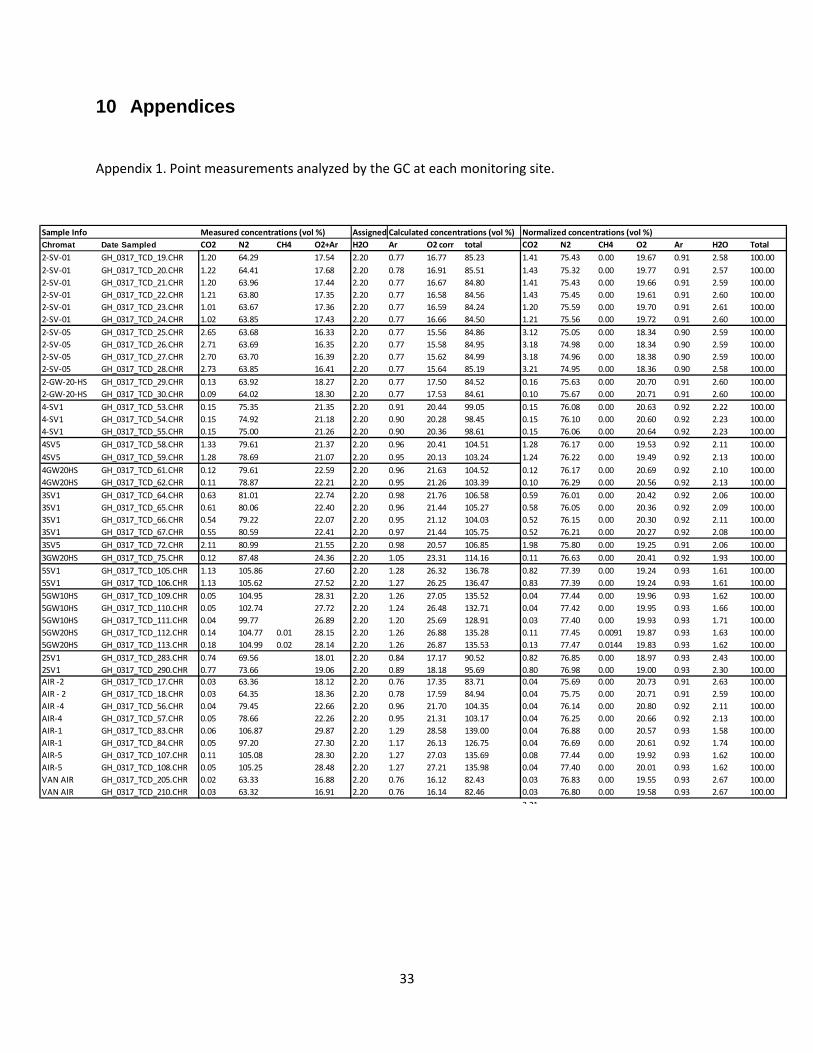
33

10 Appendices

Appendix 1. Point measurements analyzed by the GC at each monitoring site.

Sample Info Assigned (vol %)

Chromat Date Sampled CO2 N2 CH4 O2+Ar H2O Ar O2 corr total CO2 N2 CH4 O2 Ar H2O Total

2-SV-01 GH_0317_TCD_19.CHR 1.20 64.29 17.54 2.20 0.77 16.77 85.23 1.41 75.43 0.00 19.67 0.91 2.58 100.00

2-SV-01 GH_0317_TCD_20.CHR 1.22 64.41 17.68 2.20 0.78 16.91 85.51 1.43 75.32 0.00 19.77 0.91 2.57 100.00

2-SV-01 GH_0317_TCD_21.CHR 1.20 63.96 17.44 2.20 0.77 16.67 84.80 1.41 75.43 0.00 19.66 0.91 2.59 100.00

2-SV-01 GH_0317_TCD_22.CHR 1.21 63.80 17.35 2.20 0.77 16.58 84.56 1.43 75.45 0.00 19.61 0.91 2.60 100.00

2-SV-01 GH_0317_TCD_23.CHR 1.01 63.67 17.36 2.20 0.77 16.59 84.24 1.20 75.59 0.00 19.70 0.91 2.61 100.00

2-SV-01 GH_0317_TCD_24.CHR 1.02 63.85 17.43 2.20 0.77 16.66 84.50 1.21 75.56 0.00 19.72 0.91 2.60 100.00

2-SV-05 GH_0317_TCD_25.CHR 2.65 63.68 16.33 2.20 0.77 15.56 84.86 3.12 75.05 0.00 18.34 0.90 2.59 100.00

2-SV-05 GH_0317_TCD_26.CHR 2.71 63.69 16.35 2.20 0.77 15.58 84.95 3.18 74.98 0.00 18.34 0.90 2.59 100.00

2-SV-05 GH_0317_TCD_27.CHR 2.70 63.70 16.39 2.20 0.77 15.62 84.99 3.18 74.96 0.00 18.38 0.90 2.59 100.00

2-SV-05 GH_0317_TCD_28.CHR 2.73 63.85 16.41 2.20 0.77 15.64 85.19 3.21 74.95 0.00 18.36 0.90 2.58 100.00

2-GW-20-HS GH_0317_TCD_29.CHR 0.13 63.92 18.27 2.20 0.77 17.50 84.52 0.16 75.63 0.00 20.70 0.91 2.60 100.00

2-GW-20-HS GH_0317_TCD_30.CHR 0.09 64.02 18.30 2.20 0.77 17.53 84.61 0.10 75.67 0.00 20.71 0.91 2.60 100.00

4-SV1 GH_0317_TCD_53.CHR 0.15 75.35 21.35 2.20 0.91 20.44 99.05 0.15 76.08 0.00 20.63 0.92 2.22 100.00

4-SV1 GH_0317_TCD_54.CHR 0.15 74.92 21.18 2.20 0.90 20.28 98.45 0.15 76.10 0.00 20.60 0.92 2.23 100.00

4-SV1 GH_0317_TCD_55.CHR 0.15 75.00 21.26 2.20 0.90 20.36 98.61 0.15 76.06 0.00 20.64 0.92 2.23 100.00

4SV5 GH_0317_TCD_58.CHR 1.33 79.61 21.37 2.20 0.96 20.41 104.51 1.28 76.17 0.00 19.53 0.92 2.11 100.00

4SV5 GH_0317_TCD_59.CHR 1.28 78.69 21.07 2.20 0.95 20.13 103.24 1.24 76.22 0.00 19.49 0.92 2.13 100.00

4GW20HS GH_0317_TCD_61.CHR 0.12 79.61 22.59 2.20 0.96 21.63 104.52 0.12 76.17 0.00 20.69 0.92 2.10 100.00

4GW20HS GH_0317_TCD_62.CHR 0.11 78.87 22.21 2.20 0.95 21.26 103.39 0.10 76.29 0.00 20.56 0.92 2.13 100.00

3SV1 GH_0317_TCD_64.CHR 0.63 81.01 22.74 2.20 0.98 21.76 106.58 0.59 76.01 0.00 20.42 0.92 2.06 100.00

3SV1 GH_0317_TCD_65.CHR 0.61 80.06 22.40 2.20 0.96 21.44 105.27 0.58 76.05 0.00 20.36 0.92 2.09 100.00

3SV1 GH_0317_TCD_66.CHR 0.54 79.22 22.07 2.20 0.95 21.12 104.03 0.52 76.15 0.00 20.30 0.92 2.11 100.00

3SV1 GH_0317_TCD_67.CHR 0.55 80.59 22.41 2.20 0.97 21.44 105.75 0.52 76.21 0.00 20.27 0.92 2.08 100.00

3SV5 GH_0317_TCD_72.CHR 2.11 80.99 21.55 2.20 0.98 20.57 106.85 1.98 75.80 0.00 19.25 0.91 2.06 100.00

3GW20HS GH_0317_TCD_75.CHR 0.12 87.48 24.36 2.20 1.05 23.31 114.16 0.11 76.63 0.00 20.41 0.92 1.93 100.00

5SV1 GH_0317_TCD_105.CHR 1.13 105.86 27.60 2.20 1.28 26.32 136.78 0.82 77.39 0.00 19.24 0.93 1.61 100.00

5SV1 GH_0317_TCD_106.CHR 1.13 105.62 27.52 2.20 1.27 26.25 136.47 0.83 77.39 0.00 19.24 0.93 1.61 100.00

5GW10HS GH_0317_TCD_109.CHR 0.05 104.95 28.31 2.20 1.26 27.05 135.52 0.04 77.44 0.00 19.96 0.93 1.62 100.00

5GW10HS GH_0317_TCD_110.CHR 0.05 102.74 27.72 2.20 1.24 26.48 132.71 0.04 77.42 0.00 19.95 0.93 1.66 100.00

5GW10HS GH_0317_TCD_111.CHR 0.04 99.77 26.89 2.20 1.20 25.69 128.91 0.03 77.40 0.00 19.93 0.93 1.71 100.00

5GW20HS GH_0317_TCD_112.CHR 0.14 104.77 0.01 28.15 2.20 1.26 26.88 135.28 0.11 77.45 0.0091 19.87 0.93 1.63 100.00

5GW20HS GH_0317_TCD_113.CHR 0.18 104.99 0.02 28.14 2.20 1.26 26.87 135.53 0.13 77.47 0.0144 19.83 0.93 1.62 100.00

2SV1 GH_0317_TCD_283.CHR 0.74 69.56 18.01 2.20 0.84 17.17 90.52 0.82 76.85 0.00 18.97 0.93 2.43 100.00

2SV1 GH_0317_TCD_290.CHR 0.77 73.66 19.06 2.20 0.89 18.18 95.69 0.80 76.98 0.00 19.00 0.93 2.30 100.00

AIR -2 GH_0317_TCD_17.CHR 0.03 63.36 18.12 2.20 0.76 17.35 83.71 0.04 75.69 0.00 20.73 0.91 2.63 100.00

AIR - 2 GH_0317_TCD_18.CHR 0.03 64.35 18.36 2.20 0.78 17.59 84.94 0.04 75.75 0.00 20.71 0.91 2.59 100.00

AIR -4 GH_0317_TCD_56.CHR 0.04 79.45 22.66 2.20 0.96 21.70 104.35 0.04 76.14 0.00 20.80 0.92 2.11 100.00

AIR-4 GH_0317_TCD_57.CHR 0.05 78.66 22.26 2.20 0.95 21.31 103.17 0.04 76.25 0.00 20.66 0.92 2.13 100.00

AIR-1 GH_0317_TCD_83.CHR 0.06 106.87 29.87 2.20 1.29 28.58 139.00 0.04 76.88 0.00 20.57 0.93 1.58 100.00

AIR-1 GH_0317_TCD_84.CHR 0.05 97.20 27.30 2.20 1.17 26.13 126.75 0.04 76.69 0.00 20.61 0.92 1.74 100.00

AIR-5 GH_0317_TCD_107.CHR 0.11 105.08 28.30 2.20 1.27 27.03 135.69 0.08 77.44 0.00 19.92 0.93 1.62 100.00

AIR-5 GH_0317_TCD_108.CHR 0.05 105.25 28.48 2.20 1.27 27.21 135.98 0.04 77.40 0.00 20.01 0.93 1.62 100.00

VAN AIR GH_0317_TCD_205.CHR 0.02 63.33 16.88 2.20 0.76 16.12 82.43 0.03 76.83 0.00 19.55 0.93 2.67 100.00

VAN AIR GH_0317_TCD_210.CHR 0.03 63.32 16.91 2.20 0.76 16.14 82.46 0.03 76.80 0.00 19.58 0.93 2.67 100.00

3.21

Measured concentrations (vol %) Calculated concentrations (vol %) Normalized concentrations (vol %)

34

Appendix 2. All soil vapour measurements including on-site GC, sensors, and samples collected in gas

bags and canisters and analyzed in the laboratory.

CO

2O

2C

H4

N2

Po

int

me

asu

rem

en

tsB

ulk

me

asu

rem

en

tsP

oin

t m

eas

ure

me

nts

Bu

lk m

eas

ure

me

nts

Po

int

me

asu

rem

en

tsB

ulk

me

asu

rem

en

tsP

oin

t m

eas

ure

me

nts

Bu

lk m

eas

ure

me

nts

Fie

ld G

CSe

nso

rLa

b M

eas

Lab

Cal

cFi

eld

GC

Sen

sor

Lab

Me

asLa

b C

alc

Fie

ld G

CSe

nso

rLa

b M

eas

Lab

Cal

cFi

eld

GC

Sen

sor

Lab

Me

asLa

b C

alc

GH

-031

7-2-

SVI

1.20

1.20

1.18

1.01

19.7

119

.70

19.8

617

.51

0.00

0.33

0.00

0.00

75.5

775

.67

75.8

978

.45

GH

-031

7-2-

SV5

3.17

2.60

2.71

2.88

18.3

518

.80

18.5

618

.60

0.00

0.03

0.00

0.00

74.9

875

.48

75.6

775

.48

GH

-031

7-3-

SVI

0.55

0.40

0.50

0.37

20.3

420

.80

20.0

919

.87

0.00

0.00

0.00

0.00

76.1

075

.70

76.3

576

.73

GH

-031

7-3-

SV5

1.98

1.50

1.73

1.83

19.2

519

.90

19.4

318

.89

0.00

0.00

0.00

0.00

75.8

075

.50

75.7

776

.25

GH

-031

7-4-

SVI

0.15

0.30

0.17

0.17

20.6

220

.30

20.7

519

.97

0.00

0.00

0.00

0.00

76.0

876

.30

76.0

176

.83

GH

-031

7-4-

SV5

1.34

1.00

1.07

1.11

19.5

219

.50

19.7

719

.17

0.00

0.01

0.00

0.00

76.1

076

.40

76.1

076

.69

GH

-031

7-5-

SVI*

0.82

0.80

0.83

0.89

19.2

420

.60

20.1

719

.37

0.00

0.00

0.00

0.00

77.3

975

.50

75.9

476

.71

GH

-031

7-2-

GW

20-H

S0.

130.

000.

1220

.71

20.8

020

.24

0.00

0.00

0.00

75.6

576

.10

76.5

9

GH

-031

7-3-

GW

20-H

S0.

110.

100.

1220

.41

21.1

020

.37

0.00

0.00

0.00

76.6

375

.70

76.4

5

GH

-031

7-4-

GW

20-H

S0.

110.

200.

1220

.63

20.4

020

.82

0.03

0.05

0.00

76.2

376

.25

75.9

9

GH

-031

7-5-

GW

20-H

S0.

120.

1919

.85

20.7

00.

010.

0177

.46

76.0

3

GH

-031

7-5-

GW

10-H

S0.

040.

100.

040.

0519

.95

20.9

019

.95

19.6

80.

000.

0077

.42

75.9

077

.42

77.2

4

GH

-031

7-5-

AIR

0.04

0.05

0.05

20.3

120

.43

19.6

80.

000.

000.

0076

.59

76.4

577

.24

35

Appendix 3. Long term sensor and GC data for Site 2 SV01.

Sensor GC

Time CO2 O2 N2 by diff Time CO2 O2 N2 ΔCO2 ΔO2 ΔN2

3/3/17 7:20 1.21 19.10 76.49 3/03/1707:21:43 1.07 19.95 76.00 -0.14 0.85 -0.49

3/3/17 7:50 1.21 19.10 76.59 3/03/1707:51:43 1.10 19.99 75.93 -0.11 0.89 -0.66

3/3/17 8:20 1.23 19.03 76.64 3/03/1708:21:43 1.07 19.96 76.00 -0.16 0.93 -0.64

3/3/17 8:50 1.26 19.01 76.63 3/03/1708:51:43 1.07 20.01 75.98 -0.18 1.00 -0.65

3/3/17 9:20 1.27 18.97 76.66 3/03/1709:21:43 1.06 20.02 75.95 -0.21 1.05 -0.72

3/3/17 9:50 1.27 18.95 76.68 3/03/1709:51:43 1.10 19.91 76.00 -0.16 0.96 -0.68

3/3/17 10:20 1.27 18.96 76.67 3/03/1710:21:43 1.10 19.98 75.93 -0.17 1.02 -0.74

3/3/17 10:50 1.26 18.95 76.69 3/03/1710:51:44 1.08 20.02 75.92 -0.18 1.07 -0.77

3/3/17 11:20 1.26 18.96 76.68 3/03/1711:21:44 1.04 20.02 75.96 -0.23 1.06 -0.71

3/3/17 11:50 1.26 19.04 76.60 3/03/1711:51:44 1.05 20.06 76.02 -0.21 1.02 -0.58

3/3/17 12:20 1.25 18.93 76.72 3/03/1712:21:44 1.03 20.08 75.96 -0.23 1.15 -0.75

3/3/17 12:50 1.25 18.97 76.69 3/03/1712:51:44 0.94 20.12 75.95 -0.30 1.15 -0.73

3/3/17 13:20 1.25 18.96 76.69 3/03/1713:21:44 1.00 20.06 75.95 -0.25 1.10 -0.74

3/3/17 13:50 1.24 18.96 76.71 3/03/1713:51:45 0.98 20.12 75.89 -0.26 1.16 -0.82

3/3/17 14:20 1.25 18.93 76.72 3/03/1714:21:45 0.98 20.07 75.93 -0.27 1.14 -0.79

3/3/17 14:50 1.24 18.92 76.74 3/03/1714:51:45 0.99 20.07 75.93 -0.25 1.15 -0.80

3/3/17 15:20 1.23 18.92 76.75 3/03/1715:21:45 0.98 20.07 75.98 -0.25 1.15 -0.77

3/3/17 15:50 1.17 19.00 76.73 3/03/1715:51:45 0.91 20.08 75.97 -0.27 1.08 -0.76

3/3/17 16:20 1.14 19.06 76.70 3/03/1716:21:45 0.91 20.14 75.91 -0.23 1.08 -0.79

3/3/17 16:40 1.14 19.05 76.71 3/03/1716:51:45 0.89 20.13 75.93 -0.25 1.08 -0.77

3/3/17 17:10 1.17 19.01 76.72 3/03/1717:21:45 0.94 20.10 75.93 -0.23 1.09 -0.79

3/3/17 17:40 1.19 19.00 76.71 3/03/1717:51:46 0.91 20.13 75.90 -0.27 1.13 -0.81

3/3/17 18:10 1.16 19.03 76.71 3/03/1714:21:46 0.96 20.10 75.90 -0.20 1.07 -0.81

3/3/17 18:40 1.17 19.03 76.70 3/03/1714:51:46 0.92 20.16 75.86 -0.24 1.13 -0.84

3/3/17 19:10 1.19 19.01 76.70 3/03/1715:21:46 0.94 20.11 75.94 -0.25 1.10 -0.76

3/3/17 19:40 1.18 19.03 76.69 3/03/1715:51:46 0.99 20.14 75.84 -0.19 1.11 -0.85

3/3/17 20:10 1.18 19.02 76.70 3/03/1716:21:46 0.89 20.16 75.90 -0.29 1.14 -0.79

3/3/17 20:40 1.20 19.04 76.66 3/03/1716:51:46 1.00 20.01 75.93 -0.20 0.97 -0.73

3/3/17 21:10 1.21 19.02 76.67 3/03/1717:21:46 0.98 20.03 75.91 -0.23 1.01 -0.76

3/3/17 21:40 1.22 19.06 76.63 3/03/1717:51:47 1.08 19.91 75.93 -0.14 0.85 -0.70

3/3/17 22:10 1.21 19.04 76.65 3/03/1718:21:47 1.15 19.90 75.89 -0.06 0.86 -0.76

3/3/17 22:40 1.22 19.03 76.65 3/03/1718:51:47 1.10 19.95 75.88 -0.12 0.92 -0.78

3/3/17 22:50 1.22 19.05 76.63 3/03/1719:21:47 1.10 19.94 75.89 -0.12 0.89 -0.74

3/3/17 23:20 1.21 19.06 76.63 3/03/1719:51:47 1.08 19.98 75.84 -0.14 0.92 -0.79

3/3/17 23:50 1.22 19.03 76.65 3/03/1720:21:47 1.10 19.91 75.87 -0.12 0.88 -0.78

36

Appendix 4. Long term sensor and GC data for Site 2 SV05.

Sensor GC

Time CO2 O2 N2 by diff Time CO2 O2 N2 ΔCO2 ΔO2 ΔN2

03-Mar-17 18:50:00 1.17 19.02 76.70 3/03/17 18:51:44 2.65 18.31 76.60 1.48 -0.71 -0.11

03-Mar-17 19:20:00 1.19 19.04 76.67 3/03/17 19:21:44 2.70 18.41 76.45 1.51 -0.63 -0.22

03-Mar-17 19:50:00 1.18 19.04 76.68 3/03/17 19:51:44 2.73 18.37 76.56 1.55 -0.67 -0.12

03-Mar-17 20:20:00 1.19 19.01 76.70 3/03/17 20:21:44 2.70 18.32 76.63 1.51 -0.69 -0.07

03-Mar-17 20:50:00 1.20 19.03 76.67 3/03/17 20:51:44 2.71 18.32 76.61 1.50 -0.71 -0.06

03-Mar-17 21:20:00 1.21 19.04 76.65 3/03/17 21:21:44 2.73 18.35 76.59 1.52 -0.69 -0.06

03-Mar-17 21:50:00 1.21 19.03 76.66 3/03/17 21:51:44 2.73 18.37 76.56 1.51 -0.66 -0.09

03-Mar-17 22:20:00 1.21 19.04 76.65 3/03/17 22:21:44 2.71 18.40 76.57 1.50 -0.64 -0.08

03-Mar-17 22:50:00 1.22 19.05 76.63 3/03/17 22:51:45 2.71 18.36 76.63 1.49 -0.69 0.00

03-Mar-17 23:20:00 1.21 19.06 76.63 3/03/17 23:21:45 2.73 18.36 76.58 1.52 -0.70 -0.05

03-Mar-17 23:50:00 1.22 19.03 76.65 3/03/17 23:51:45 2.76 18.36 76.56 1.54 -0.67 -0.09

04-Mar-17 00:20:00 1.22 19.02 76.66 3/04/17 00:21:45 2.79 18.35 76.55 1.56 -0.67 -0.10

04-Mar-17 00:50:00 1.22 19.04 76.64 3/04/17 00:51:45 2.76 18.36 76.56 1.55 -0.68 -0.08

04-Mar-17 01:20:00 1.22 19.04 76.64 3/04/17 01:21:45 2.77 18.39 76.52 1.56 -0.65 -0.13

04-Mar-17 01:50:00 1.22 19.06 76.62 3/04/17 01:51:46 2.78 18.37 76.53 1.56 -0.69 -0.09

04-Mar-17 02:20:00 1.22 19.05 76.63 3/04/17 02:21:46 2.74 18.33 76.64 1.52 -0.72 0.01

04-Mar-17 02:50:00 1.22 19.06 76.62 3/04/17 02:51:46 2.77 18.34 76.59 1.55 -0.72 -0.03

04-Mar-17 03:20:00 1.23 19.03 76.64 3/04/17 03:21:46 2.75 18.36 76.62 1.52 -0.67 -0.03

04-Mar-17 03:50:00 1.22 19.15 76.53 3/04/17 03:51:46 2.77 18.33 76.60 1.56 -0.82 0.07

04-Mar-17 04:20:00 1.22 19.15 76.53 3/04/17 04:21:46 2.80 18.33 76.57 1.58 -0.82 0.03

04-Mar-17 04:50:00 1.21 19.07 76.62 3/04/17 04:51:46 2.78 18.31 76.60 1.57 -0.76 -0.02

04-Mar-17 05:20:00 1.21 19.10 76.59 3/04/17 05:21:46 2.78 18.31 76.59 1.57 -0.79 0.00

04-Mar-17 05:50:00 1.21 19.09 76.60 3/04/17 05:51:47 2.79 18.31 76.58 1.58 -0.78 -0.03

04-Mar-17 06:20:00 1.20 19.09 76.61 3/04/17 06:21:47 2.82 18.28 76.57 1.61 -0.81 -0.04

04-Mar-17 06:50:00 1.20 19.17 76.53 3/04/17 06:51:47 2.78 18.32 76.57 1.58 -0.85 0.04

04-Mar-17 07:20:00 1.20 19.19 76.51 3/04/17 07:21:47 2.81 18.32 76.55 1.61 -0.87 0.04

04-Mar-17 07:50:00 1.21 19.11 76.58 3/04/17 07:51:47 2.81 18.31 76.56 1.60 -0.80 -0.03

04-Mar-17 08:20:00 1.20 19.16 76.54 3/04/17 08:21:47 2.79 18.32 76.58 1.59 -0.84 0.04

04-Mar-17 08:50:00 1.21 19.07 76.62 3/04/17 08:51:47 2.81 18.32 76.55 1.60 -0.75 -0.07

04-Mar-17 09:20:00 1.22 19.05 76.63 3/04/17 09:21:47 2.83 18.33 76.52 1.61 -0.72 -0.11

04-Mar-17 09:50:00 1.23 19.09 76.58 3/04/17 09:51:48 2.80 18.36 76.53 1.57 -0.73 -0.05

04-Mar-17 10:20:00 1.24 19.08 76.58 3/04/17 10:21:48 2.81 18.36 76.53 1.57 -0.72 -0.05

04-Mar-17 10:50:00 1.24 19.02 76.64 3/04/17 10:51:48 2.77 18.36 76.56 1.53 -0.66 -0.08

0.00

5.00

10.00

15.00

20.00

25.00

0.00

initial site characterisation and assessment of

Documents