insight into the flow-condition-based interpolation finite...
TRANSCRIPT
INTERNATIONAL JOURNAL FOR NUMERICAL METHODS IN ENGINEERINGInt. J. Numer. Meth. Engng 2005; 63:197–217Published online 15 February 2005 in Wiley InterScience (www.interscience.wiley.com). DOI: 10.1002/nme.1276
Insight into the flow-condition-based interpolation finite elementapproach: solution of steady-state advection–diffusion problems
Haruhiko Kohno and Klaus Jürgen Bathe∗,†
Department of Mechanical Engineering, Massachusetts Institute of Technology, 77 Massachusetts Avenue,Cambridge, MA, 02139-4307, U.S.A.
SUMMARY
The flow-condition-based interpolation (FCBI) finite element approach is studied in the solution ofadvection–diffusion problems. Two FCBI procedures are developed and tested with the original FCBImethod: in the first scheme, a general solution of the advection–diffusion equation is embedded into theinterpolation, and in the second scheme, the link-cutting bubbles approach is used in the interpolation.In both procedures, as in the original FCBI method, no artificial parameters are included to reachstability for high Péclet number flows. The procedures have been implemented for two-dimensionalanalysis and the results of some test problems are presented. These results indicate good stabilityand accuracy characteristics and the potential of the FCBI solution approach. Copyright � 2005John Wiley & Sons, Ltd.
KEY WORDS: advection–diffusion; stabilization; flow-condition-based interpolations
1. INTRODUCTION
The numerical solution of high Péclet and high Reynolds number flows is of great importance inresearch and industry. For this reason and because the development presents a great challenge,a very large research effort has been focused on improving the methods of solution over thelast decades, and this effort is still continuing very widely.
The finite element method is clearly the most effective numerical solution technique for theanalysis of solids and structures [1, 2]. However, considering fluid flows, while much researchhas been focused on the development of finite element methods (see, e.g. References [1–7]),finite difference, finite volume and spectral methods are still considerably more effective inmost practical applications. Indeed, almost all fluid flow problems in industry are still solved
∗Correspondence to: K. J. Bathe, Department of Mechanical Engineering, Massachusetts Institute of Technology,77 Massachusetts Avenue, Cambridge, MA, 02139-4307, U.S.A.
†E-mail: [email protected]
Contract/grant sponsor: Ministry of Education, Culture, Sports, Science and Technology (MEXT), Japan
Received 5 May 2004Revised 9 July 2004
Copyright � 2005 John Wiley & Sons, Ltd. Accepted 8 November 2004
198 H. KOHNO AND K. J. BATHE
using finite volume techniques. On the other hand, if a finite element method were availablethat is clearly more effective, then such a method would find wide usage.
We have focused our research on the development of the flow-condition-based interpolation(FCBI) procedure [8–10] for the finite element solution of incompressible fluid flows, includingfluid–structure interactions. This method might be referred to as a hybrid of the traditional finiteelement and finite volume methods. The key aspects of the FCBI procedure are that, firstly,finite element interpolations considering flow conditions are used which lead to stability and,secondly, local flux equilibrium (that is, mass and momentum conservation) is satisfied. Ourobjective in this development is to reach a method that is more effective in stability, accuracyand computational effort than the traditional finite element and finite volume techniques.
Specifically, the basic aim in our development is to reach a numerical scheme that is stablewith optimal accuracy characteristics, for low and high Péclet and Reynolds number flows[8–11]. In particular, considering a high Reynolds number flow, the scheme should give areasonable solution, even when using a rather coarse mesh and without the use of artificialsolution parameters. The global flow characteristics should be correctly displayed, and in fluid–structure interactions, the tractions on the structural surfaces should be reasonable. As the fluidmesh is then refined, more details of the flow should be revealed, and ideally the numericalsolution would converge with optimum rate to the ‘exact’ solution of the mathematical model.In practice, of course, the solution of the Navier–Stokes equations at high Reynolds numberwould not be obtained with high accuracy. The mesh would have to be too fine. Instead, aturbulence model would be used at some stage of mesh refinement. However, the solutionproperty that stability is preserved at high Reynolds and Péclet number flows with coarsemeshes and optimal accuracy is of much value in practical analysis.
The possible use of coarse meshes without artificial solution parameters implies that ananalyst does not need to spend undue effort on meshing the domain and experimenting withnumerical parameters merely to obtain a first reasonable flow solution. Also, if a discretizationscheme is employed with goal-oriented error measures [12], then it is assumed that solutionscan directly be obtained for all meshes used. The goal-oriented discretization approach isparticularly valuable in the solution of fluid–structure interactions where the fluid mesh onlyneeds to be fine enough to solve accurately for the pressure/tractions on the structure.
The basic philosophy of our developments was presented earlier [8–10], and the FCBIapproach is already quite widely used [10]. However, we are of course aiming to furtherstudy the solution properties and increase the effectiveness of the original procedure. Sincethe method is a hybrid of the finite element and finite volume techniques, the FCBI schemeis naturally also related to the much researched streamline upwind/Petrov–Galerkin (SUPG)method [3], the Galerkin/least-squares (GLS) method [4], the use of bubble functions [6], andother schemes [1, 2, 7]. However, a distinguishing feature is that an analytical solution of theone-dimensional advection–diffusion equation (to stabilize the convective terms in the Galerkinformulation) is used over a control volume, and hence the FCBI method is also related to thecubic interpolated pseudoparticle/propagation (CIP) method [13].
The objective of this paper is to study the spatial solution accuracy of the original FCBIscheme [9] and two variations thereof for advection–diffusion problems in order to obtainfurther insight into the solution approach. Whereas in the original FCBI scheme one-dimensionalanalytical flow conditions are used in two- and three-dimensional interpolations, we considerhere, in an additional FCBI scheme, a general two-dimensional solution. Furthermore, in a thirdscheme we embed the interpolations of the link-cutting bubbles proposed by Brezzi et al. [14]
Copyright � 2005 John Wiley & Sons, Ltd. Int. J. Numer. Meth. Engng 2005; 63:197–217
FLOW-CONDITION-BASED INTERPOLATION FINITE ELEMENT APPROACH 199
into the FCBI approach. In the paper, we first present the numerical procedures used and thengive the solutions of various test problems. The numerical experiments indicate the stabilityand accuracy of the FCBI procedures and also show that the FCBI approach has significantfurther potential to reach improved solution methods.
2. FCBI METHODS FOR ADVECTION–DIFFUSION PROBLEMS
In this section we review the original FCBI method and introduce two additional FCBI proce-dures. We consider an incompressible flow advection–diffusion problem in a two-dimensionaldomain in which the velocity is prescribed. A steady-state analysis is carried out with Dirichletboundary conditions. We assume that the problem is well-posed in the Hilbert space �. Thenon-dimensional governing equation in conservative form is:
Find the temperature �(x) ∈ � such that
∇·(
v� − 1
Pe∇�
)= 0, x ∈ � (1)
where v is the prescribed velocity and � ∈ �2 is a domain with boundary S = S̄�. The Pécletnumber is defined as Pe = UL/�; U , L and � are the representative velocity, the representativelength and the thermal diffusivity, respectively. The above equation is subject to the followingboundary condition:
� = �s , x ∈ S̄� (2)
where �s is the prescribed temperature on the boundary S̄�.
2.1. The original method
For the finite element solution, we use a Petrov–Galerkin variational formulation with subspaces�h, �h and Wh of � of the problem in Equations (1) and (2). The formulation for the numericalsolution is
Find � ∈ �h, � ∈ �h such that for all w ∈ Wh∫�
w
{∇·(
v� − 1
Pe∇�
)}d� = 0 (3)
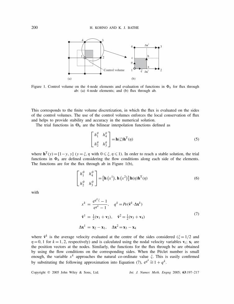
Figure 1(a) shows a mesh of elements in the natural co-ordinate system. Here, both velocityand temperature are defined at each node of the 4-node elements.
The weight functions in the space Wh are step functions. For example, we have at node 1in Figure 1(b),
hw1 =
{1 (�, �) ∈ [0, 1
2
]× [0, 12
]0 else
(4)
Copyright � 2005 John Wiley & Sons, Ltd. Int. J. Numer. Meth. Engng 2005; 63:197–217
200 H. KOHNO AND K. J. BATHE
Control volume 1
4
a
bc
ξ
η
1 2
1x∆
2x∆
4 3
2
3
(a) (b)
Figure 1. Control volume on the 4-node elements and evaluation of functions in �h for flux throughab: (a) 4-node elements; and (b) flux through ab.
This corresponds to the finite volume discretization, in which the flux is evaluated on the sidesof the control volumes. The use of the control volumes enforces the local conservation of fluxand helps to provide stability and accuracy in the numerical solution.
The trial functions in �h are the bilinear interpolation functions defined as h�
1 h�4
h�2 h�
3
= h(�)hT(�) (5)
where hT(y) = [1−y, y] (y = �, � with 0 � �, � � 1). In order to reach a stable solution, the trialfunctions in �h are defined considering the flow conditions along each side of the elements.The functions are for the flux through ab in Figure 1(b),
h�1 h
�4
h�2 h
�3
= [h (x1), h
(x2)]h(�)hT(�) (6)
with
xk = eqk� − 1
eqk − 1, qk = Pe(v̄k ·�xk)
v̄1 = 12(v1 + v2), v̄2 = 1
2(v3 + v4)
�x1 = x2 − x1, �x2 = x3 − x4
(7)
where v̄k is the average velocity evaluated at the centre of the sides considered (� = 1/2 and� = 0, 1 for k = 1, 2, respectively) and is calculated using the nodal velocity variables vi ; xi arethe position vectors at the nodes. Similarly, the functions for the flux through bc are obtainedby using the flow conditions on the corresponding sides. When the Péclet number is smallenough, the variable xk approaches the natural co-ordinate value �. This is easily confirmedby substituting the following approximation into Equation (7), eqk ∼= 1 + qk .
Copyright � 2005 John Wiley & Sons, Ltd. Int. J. Numer. Meth. Engng 2005; 63:197–217
FLOW-CONDITION-BASED INTERPOLATION FINITE ELEMENT APPROACH 201
Using Equations (5)–(7) the temperatures � and � are, respectively, calculated with the trialfunctions in �h and �h as follows:
� = h�i �i (8)
� = h�i �i (9)
where �i are the nodal temperature variables. The trial functions used here satisfy the require-ment �hi = 1. The flux is calculated with the interpolated values at the centre of the sides ofthe control volumes. For example, the flux through ab is obtained as follows:∫ b
a
n · f ds = (n · f)|�=1/2,�=1/4�sab (10)
with
f(�, �) = v� − 1
Pegj ��
��j(11)
where n, �sab and gj are the unit normal vector pointing to the outside of the control volume,the length of ab and the contravariant base vector, respectively. In Equation (10), the velocityis interpolated with the trial functions in �h; v = h�
i vi .This approach of solution was first introduced into the Navier–Stokes equations with the
primary aim to have stability of the solution [9, 15], because in practice a stable and reason-able solution is ideally obtained at any Reynolds (and Péclet) number flow. Of course, wealso endeavour to have a solution as accurate as possible, and this aim motivates the furtherdevelopment of the scheme.
2.2. Using a general solution
In the advection-dominated regime, an effective stabilizing scheme is required in order toobtain reliable results with a reasonable mesh. This requirement is fulfilled in the originalFCBI method in a physically based manner by introducing the one-dimensional exact solutionof the advection–diffusion equation into the trial functions in �h as shown in Equations (6)and (7). However, since the flow conditions are estimated on the sides of the elements andthen linearly interpolated in the elements, fine grids are necessary to obtain accurate resultswhen very high Péclet number flows are analysed in multi-dimensional domains. For thisreason, possibly more efficient trial functions in �h, which are based on two-dimensional flowconditions, are considered in this section.
In two-dimensional analysis, it is not possible to obtain the exact solution of the advection–diffusion equation in an element since the exact boundary conditions on the sides are unknownas long as the temperatures are defined only at the nodes. Hence, the following trial functions arecreated by multiplying the one-dimensional exact-solution-based interpolation in the � directionby that in the � direction, which are in an analogous form with Equation (5):
h�1 h
�4
h�2 h
�3
= h(�)hT(�) (12)
Copyright � 2005 John Wiley & Sons, Ltd. Int. J. Numer. Meth. Engng 2005; 63:197–217
202 H. KOHNO AND K. J. BATHE
x
y
v
ξ
η
12
3
4
ηh
ξh
2
1=η
2
1=ξ
ηe
ξe
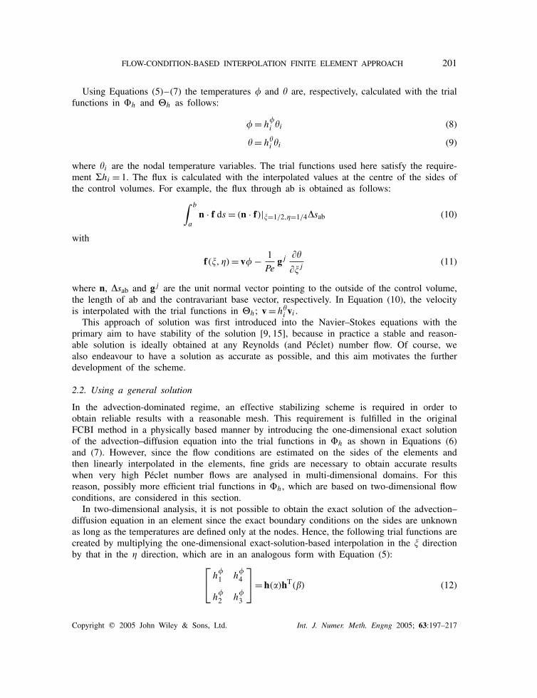
Figure 2. Illustration of the projections of velocity and the element lengths in the � and � directions.
with
� = ePee�� − 1
ePee� − 1
, � = ePee�� − 1
ePee� − 1
Pee� = Pe
(v̄ · e�
)h� = Pe v̄�h�, Pee
� = Pe(v̄ · e�
)h� = Pe v̄�h�
h� =∥∥�x1 + �x2
∥∥2
, h� =∥∥�y1 + �y2
∥∥2
(13)
�y1 = x4 − x1, �y2 = x3 − x2
where Pee� and Pee
� are the element Péclet numbers corresponding to the projections of thevelocity vector v̄ evaluated at the centre of the element onto the � and � directions, seeFigure 2.
It should be emphasized that in a rectangular element the above trial functions correspondto the two-dimensional general solution which consists of four independent basic solutionsconnected linearly as follows:
� =[1, ePee
��, ePee��, ePee
��+Pee��]
C1
C2
C3
C4
(14)
Equations (8), (12) and (13) are obtained by substituting the following boundary condi-tions into Equation (14): �1 = �(0, 0), �2 = �(1, 0), �3 = �(1, 1), �4 = �(0, 1). Note that thesetrial functions also meet the requirement �hi = 1 regardless of the element Pécletnumbers.
Copyright � 2005 John Wiley & Sons, Ltd. Int. J. Numer. Meth. Engng 2005; 63:197–217
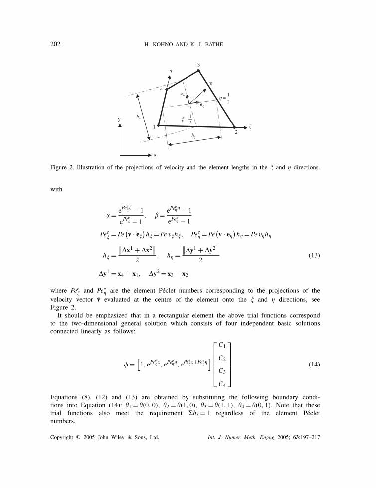
FLOW-CONDITION-BASED INTERPOLATION FINITE ELEMENT APPROACH 203
a
d b d
a
c
b
c
°45
A cd
ba Flow direction
(a) (b) (c)
Figure 3. Trial functions in �h for node A in two elements: (a) problemdefinition; (b) Pee = 1; and (c) Pee = 10.
Figure 3 shows the profiles of the trial functions for Pee = Pee� = Pee
� = 1, 10 in two ele-ments in case a 45◦ advective velocity is prescribed. When the element Péclet numbers aresmall enough, the trial functions in Equation (12) approach the bilinear interpolation func-tions in Equation (5) since ePee
� ∼= 1 + Pee�, ePee
� ∼= 1 + Pee�. Of course, using the same pro-
cedure, the proposed trial functions can, also, be developed directly for three-dimensionalsolutions.
2.3. Using link-cutting bubbles
Another approach to stabilize the solution can be established by adopting an augmented strategy,in which the finite element space is enriched by bubble functions. In this section, we proposea scheme that introduces the link-cutting bubbles [14], suitably located in the augmented spaceconsidering flow conditions, into the FCBI procedure.
Consider a one-dimensional advection–diffusion problem solved with 2-node equal lengthelements. Here, the element Péclet number is positive and we define it to be qk/2. In thiscase, the exponential scheme [16], which gives the exact solution at each node, can be writtenas follows:
−eqk/2�j−1 +(
eqk/2 + 1)
�j − �j+1 = 0 (15)
where �j−1, �j and �j+1 are the temperature variables at the consecutive nodes. Then thevariable �j is obtained in terms of �j−1 and �j+1 as follows:
�j = eqk − eqk/2
eqk − 1�j−1 + eqk/2 − 1
eqk − 1�j+1 = hT(xk(1/2)
) [ �j−1
�j+1
](16)
Note that Equation (16) contains the same vector h(xk)
that is used in Equation (6), when� = 1/2. Similarly, the following equation is obtained in the Galerkin method coupled with thelink-cutting bubbles:(
−qk
4− 1 − qk
2U
)�j−1 + 2
(1 + qk
2U
)�j +
(qk
4− 1 − qk
2U
)�j+1 = 0 (17)
Copyright � 2005 John Wiley & Sons, Ltd. Int. J. Numer. Meth. Engng 2005; 63:197–217
204 H. KOHNO AND K. J. BATHE
1 2
34
a
b
1x∆
2x∆
ξ
η
Figure 4. Evaluation of the trial functions based on link-cutting bubbles in �h for flux through ab.
where the term qkU/2 represents the stabilizing effect. Then the variable �j is obtained asfollows:
�j = qk + 4 + 2qkU
8 + 4qkU�j−1 + −qk + 4 + 2qkU
8 + 4qkU�j+1 = hT(bk
) [ �j−1
�j+1
](18)
with
bk = −qk + 4 + 2qkU
8 + 4qkU(19)
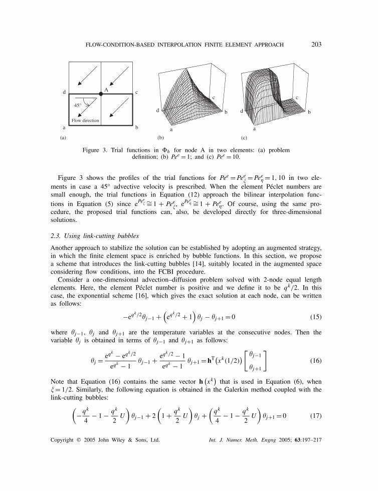
Therefore, this bubble stabilization technique can be naturally introduced into the original FCBImethod by replacing xk in Equation (7) with bk . When the link-cutting bubbles are set on thevectors �x1 and �x2 as shown in Figure 4, at � = 1/2 the trial functions in �h are for theflux through ab,
h
�1 h
�4
h�2 h
�3
= [h (b1), h
(b2)]h(�)hT(�) (20)
if uk � 0 then bk = − ∣∣qk∣∣+ 4 + 2
∣∣qk∣∣U
8 + 4∣∣qk∣∣U (21)
if uk<0 then bk =∣∣qk∣∣+ 4 + 2
∣∣qk∣∣U
8 + 4∣∣qk∣∣U (22)
with
U = d1(d1S2,2 − d2S1,2
)− d2(d1S2,1 − d2S1,1
)S1,1S2,2 − S1,2S2,1
|uk|
Copyright � 2005 John Wiley & Sons, Ltd. Int. J. Numer. Meth. Engng 2005; 63:197–217
FLOW-CONDITION-BASED INTERPOLATION FINITE ELEMENT APPROACH 205
d1 = 1
lk
(�k
2+ �k
2
), d2 = 1
lk
(�k
2+ k
2
)
S1,1 = 1
Pe
(1
�k+ 1
�k
), S1,2 = − 1
Pe�k+∣∣uk∣∣
2
S2,1 = − 1
Pe�k−∣∣uk∣∣
2, S2,2 = 1
Pe
(1
�k+ 1
k
)
lk =∥∥�xk
∥∥2
, uk = v̄k ·�xk∥∥�xk∥∥ (23)
The two-bubble subgrid is determined by putting two points, zk1, zk
2, in the half length of eachside as follows:
if6
Pe� |uk|lk then �k = k = �k = lk
3(24)
if6
Pe< |uk|lk then �k = lk − 4∣∣uk
∣∣Pe, k = �k = 2∣∣uk
∣∣Pe(25)
with
�1 = ∥∥z11 − x1
∥∥, 1 =∥∥∥∥x1 + x2
2− z1
2
∥∥∥∥, �1 = ∥∥z12 − z1
1
∥∥�2 = ∥∥z2
1 − x4∥∥, 2 =
∥∥∥∥x3 + x4
2− z2
2
∥∥∥∥, �2 = ∥∥z22 − z2
1
∥∥ (26)
when uk � 0, while the roles of these points are exchanged when uk<0. Equations (24) and(25) are based on the work of Brezzi et al. [14].
Since Equation (12) is obtained by multiplying the one-dimensional exact-solution-based in-terpolations in the � and � directions, the same strategy can also be applied to the FCBIprocedure with link-cutting bubbles. By using the one-dimensional interpolation functionsincluding link-cutting bubbles, which are evaluated on the element lengths h� and h� de-fined in Equation (13), the following trial functions in �h can be established in analogyto Equations (12) and (13):
h�1 h
�4
h�2 h
�3
= h
(�′)hT (�′) (27)
if v̄� � 0 then �′ =�
−
∣∣∣Pee�
∣∣∣2
(1 − �) + 1 +∣∣∣Pee
�
∣∣∣ (1 − �)U2�
1 +∣∣∣Pee
�
∣∣∣ �(1 − �)(U1� + U2�
) (28)
Copyright � 2005 John Wiley & Sons, Ltd. Int. J. Numer. Meth. Engng 2005; 63:197–217
206 H. KOHNO AND K. J. BATHE
if v̄�<0 then �′ =�
∣∣∣Pee
�
∣∣∣2
(1 − �) + 1 +∣∣∣Pee
�
∣∣∣ (1 − �)U1�
1 +∣∣∣Pee
�
∣∣∣ �(1 − �)(U1� + U2�
) (29)
if v̄� � 0 then �′ =�
−
∣∣∣Pee�
∣∣∣2
(1 − �) + 1 +∣∣∣Pee
�
∣∣∣ (1 − �)U2�
1 +∣∣∣Pee
�
∣∣∣ �(1 − �)(U1� + U2�
) (30)
if v̄�<0 then �′ =�
∣∣∣Pee
�
∣∣∣2
(1 − �) + 1 +∣∣∣Pee
�
∣∣∣ (1 − �)U1�
1 +∣∣∣Pee
�
∣∣∣ �(1 − �)(U1� + U2�
) (31)
with
Uir = d1(d1S2,2 − d2S1,2
)− d2(d1S2,1 − d2S1,1
)S1,1S2,2 − S1,2S2,1
∣∣∣∣∣ir
|v̄r |
(d1)ir = 1
lir
(�ir
2+ �ir
2
), (d2)ir = 1
lir
(�ir
2+ ir
2
)
(S1,1
)ir
= 1
Pe
(1
�ir
+ 1
�ir
),(S1,2
)ir
=− 1
Pe�ir
+ |v̄r |2
(S2,1
)ir
= − 1
Pe�ir
− |v̄r |2
,(S2,2
)ir
= 1
Pe
(1
�ir
+ 1
ir
)
l1� = h��, l2� = h� (1 − �)
l1� = h��, l2� = h�(1 − �)
(32)
where i = 1, 2 and r = �, �. The two-bubble subgrid in each direction is determined as follows:
if6
Pe� |v̄r | lir then �ir = ir = �ir = lir
3(33)
if6
Pe< |v̄r | lir then �ir = lir − 4
|v̄r | Pe, ir = �ir = 2
|v̄r | Pe(34)
Figure 5 gives an illustration of the trial functions in �h, as per Equation (27). In this figure,for simplicity, a rectangular element is considered. We use the scheme defined by Equation (27)in the numerical example solutions.
Copyright � 2005 John Wiley & Sons, Ltd. Int. J. Numer. Meth. Engng 2005; 63:197–217
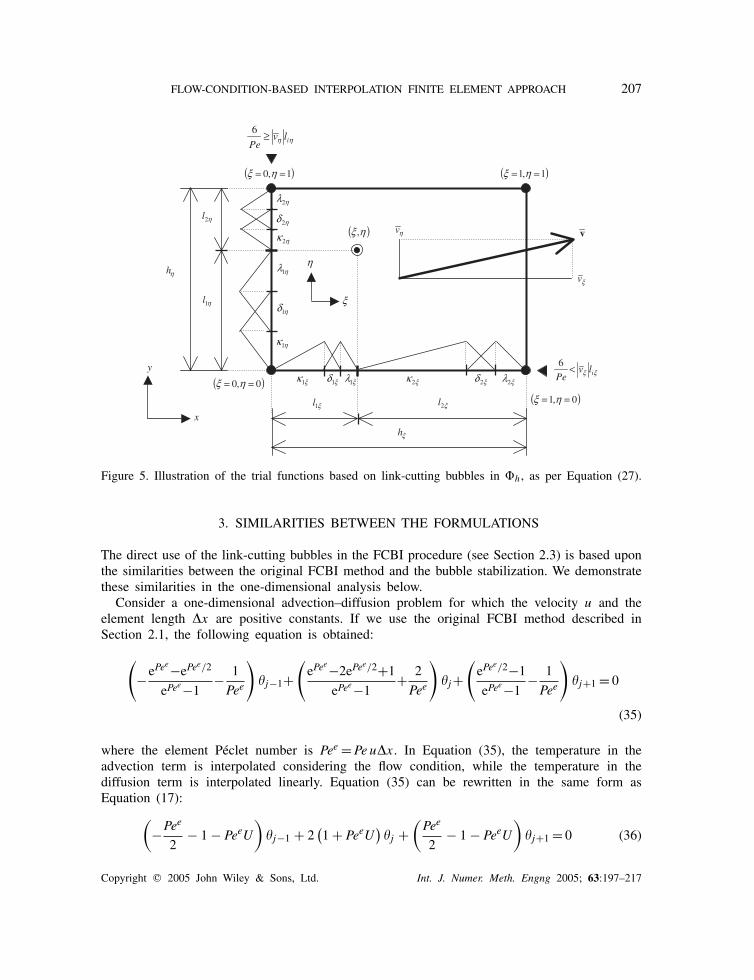
FLOW-CONDITION-BASED INTERPOLATION FINITE ELEMENT APPROACH 207
ξ
η
( )ηξ ,
ξκ1 ξδ1 ξλ1 ξκ2 ξδ2 ξλ2
v
ηκ1
ηδ1
ηλ1
ηκ2
ηδ2
ηλ2
ξh
ξ1l ξ2l
η1l
η2l
ηh
x
y
( )0,0 == ηξ( )0,1 == ηξ
( )1,1 == ηξ( )1,0 == ηξ
ξv
ηv
ηη ilvPe
≥6
ξξ ilvPe
<6
Figure 5. Illustration of the trial functions based on link-cutting bubbles in �h, as per Equation (27).
3. SIMILARITIES BETWEEN THE FORMULATIONS
The direct use of the link-cutting bubbles in the FCBI procedure (see Section 2.3) is based uponthe similarities between the original FCBI method and the bubble stabilization. We demonstratethese similarities in the one-dimensional analysis below.
Consider a one-dimensional advection–diffusion problem for which the velocity u and theelement length �x are positive constants. If we use the original FCBI method described inSection 2.1, the following equation is obtained:
(−ePee−ePee/2
ePee−1− 1
Pee
)�j−1+
(ePee−2ePee/2+1
ePee−1+ 2
Pee
)�j+
(ePee/2−1
ePee−1− 1
Pee
)�j+1 = 0
(35)
where the element Péclet number is Pee = Pe u�x. In Equation (35), the temperature in theadvection term is interpolated considering the flow condition, while the temperature in thediffusion term is interpolated linearly. Equation (35) can be rewritten in the same form asEquation (17):(
−Pee
2− 1 − PeeU
)�j−1 + 2
(1 + PeeU
)�j +
(Pee
2− 1 − PeeU
)�j+1 = 0 (36)
Copyright � 2005 John Wiley & Sons, Ltd. Int. J. Numer. Meth. Engng 2005; 63:197–217
208 H. KOHNO AND K. J. BATHE
with
U = 1 − e−Pee/2
2(1 + e−Pee/2
) (37)
Therefore, Equation (36) can also be the basis of using link-cutting bubbles by substituting forU in Equation (36):
U = d1(d1S2,2 − d2S1,2
)− d2(d1S2,1 − d2S1,1
)S1,1S2,2 − S1,2S2,1
u (38)
where uk and lk used in Equation (23) are, respectively, replaced by u and �x, and Equation (17)is obtained when Pee = qk/2.
In the advection-dominated regime, we see that in the two-bubble subgrid considered inEquation (25) Pe→∞, �→�x, = �→0, uPe� = uPe = 2. Consequently, we have
d1→ 12 , d2→0, (39)
so that Equation (38) becomes
U = d1(d1S2,2 − d2S1,2
)− d2(d1S2,1 − d2S1,1
)S1,1S2,2 − S1,2S2,1
u→1412
= 1
2(40)
As a result, Equation (36) then corresponds to ‘full upwinding.’ The same can be easily provedusing Equation (37); as Pee→∞, U→1/2. On the other hand, these stabilizing variablesapproach zero in the diffusion-dominated regime; Pee→0, U→0 in Equations (37) and (38).As a result, Equation (36) then corresponds to the formulation of the standard Galerkin methodin which linear shape functions are used.
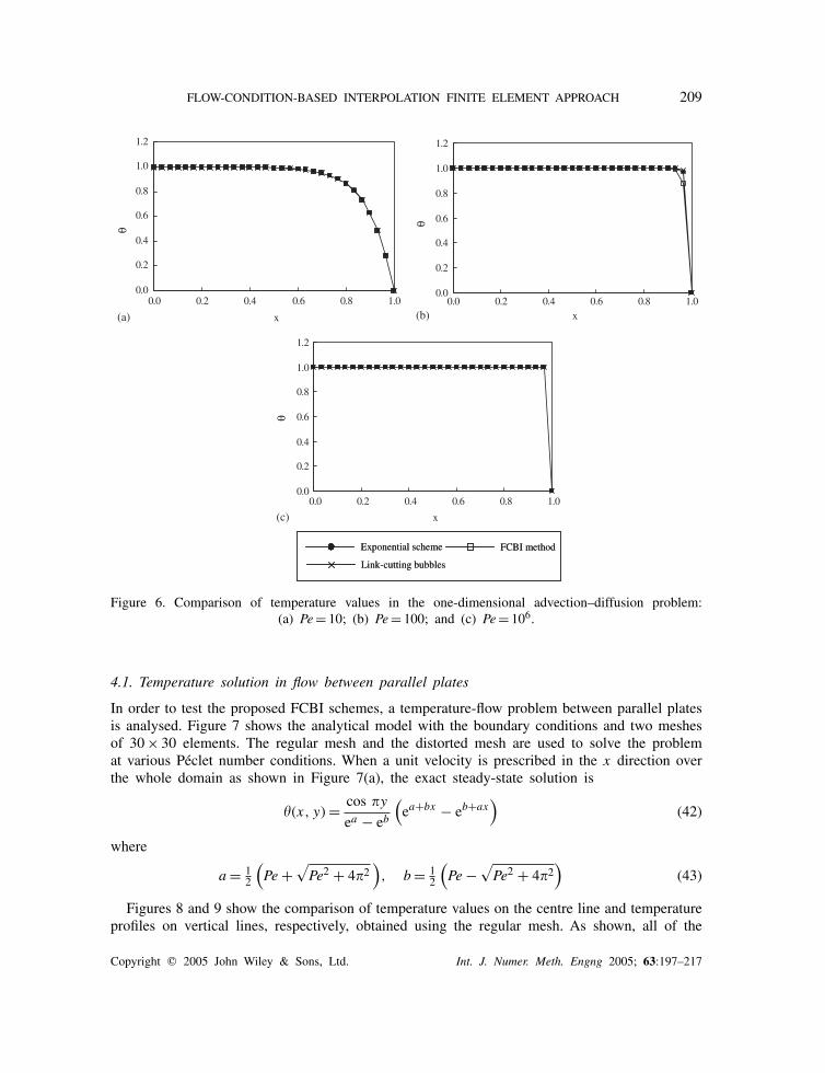
Figure 6 shows a comparison of temperature distributions obtained using the exponentialscheme, the FCBI method (Equation (35)) and the link-cutting bubbles scheme (Equations (36)and (38)) for the conditions Pe = 10, 100 and 106. The boundary conditions are
� = 1 at x = 0
� = 0 at x = 1(41)
The solution is obtained with 30 2-node equal-length elements. As shown, good agreement isobtained in the solution for a wide range of Péclet number problems. The small error in theFCBI temperature solution near x = 1 when Pe = 100 is due to using the linear temperatureinterpolation in the diffusion term.
4. NUMERICAL EXAMPLES
In this section we present some solution results that we use to study the stability and accuracyof the FCBI schemes.
Copyright � 2005 John Wiley & Sons, Ltd. Int. J. Numer. Meth. Engng 2005; 63:197–217
FLOW-CONDITION-BASED INTERPOLATION FINITE ELEMENT APPROACH 209
0.0
0.2
0.4
0.6
0.8
1.0
1.2
0.0 0.2 0.4 0.6 0.8 1.0
0.0
0.2
0.4
0.6
0.8
1.0
1.2
0.0 0.2 0.4 0.6 0.8 1.00.0
0.2
0.4
0.6
0.8
1.0
1.2
0.0 0.2 0.4 0.6 0.8 1.0
x
Exponential scheme FCBI method
Link-cutting bubbles
Exponential scheme FCBI method
Link-cutting bubbles
(a) x(b)
x(c)
θ θ
θ
Figure 6. Comparison of temperature values in the one-dimensional advection–diffusion problem:(a) Pe = 10; (b) Pe = 100; and (c) Pe = 106.
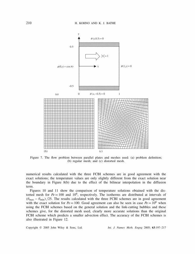
4.1. Temperature solution in flow between parallel plates
In order to test the proposed FCBI schemes, a temperature-flow problem between parallel platesis analysed. Figure 7 shows the analytical model with the boundary conditions and two meshesof 30 × 30 elements. The regular mesh and the distorted mesh are used to solve the problemat various Péclet number conditions. When a unit velocity is prescribed in the x direction overthe whole domain as shown in Figure 7(a), the exact steady-state solution is
�(x, y) = cos y
ea − eb
(ea+bx − eb+ax
)(42)
where
a = 12
(Pe +
√Pe2 + 42
), b = 1
2
(Pe −
√Pe2 + 42
)(43)
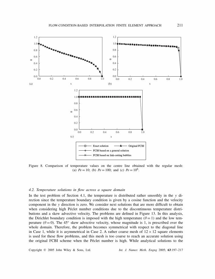
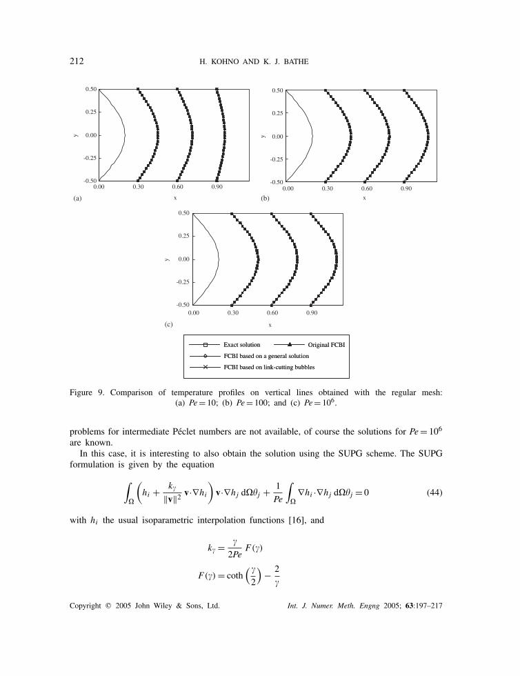
Figures 8 and 9 show the comparison of temperature values on the centre line and temperatureprofiles on vertical lines, respectively, obtained using the regular mesh. As shown, all of the
Copyright � 2005 John Wiley & Sons, Ltd. Int. J. Numer. Meth. Engng 2005; 63:197–217
210 H. KOHNO AND K. J. BATHE
(b)
(a)
(c)
x
y
0 1
θ
θ
θ
yπθ (0,y) = cos (1,y) = 0
1=v
-0.5
0.5
(x,−0.5) = 0
(x,0.5) = 0
Figure 7. The flow problem between parallel plates and meshes used: (a) problem definition;(b) regular mesh; and (c) distorted mesh.
numerical results calculated with the three FCBI schemes are in good agreement with theexact solutions; the temperature values are only slightly different from the exact solution nearthe boundary in Figure 8(b) due to the effect of the bilinear interpolation in the diffusionterm.
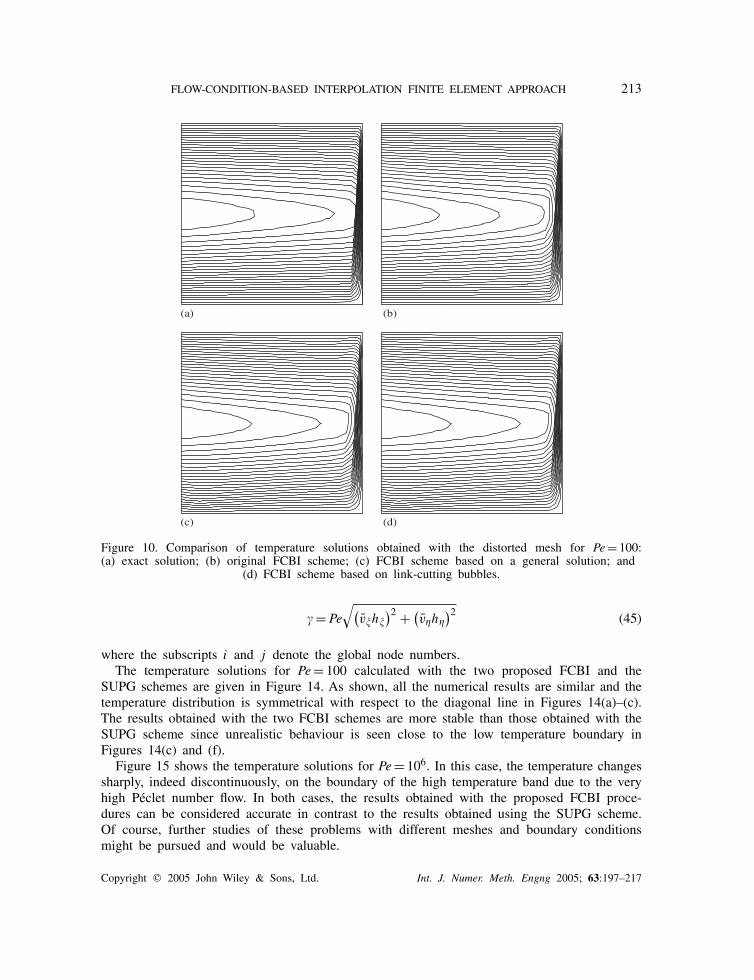
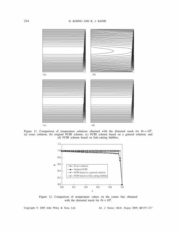
Figures 10 and 11 show the comparison of temperature solutions obtained with the dis-torted mesh for Pe = 100 and 106, respectively. The isotherms are distributed at intervals of(�max − �min) /25. The results calculated with the three FCBI schemes are in good agreementwith the exact solution for Pe = 100. Good agreement can also be seen in case Pe = 106 whenusing the FCBI schemes based on the general solution and the link-cutting bubbles and theseschemes give, for the distorted mesh used, clearly more accurate solutions than the originalFCBI scheme which predicts a smaller advection effect. The accuracy of the FCBI schemes isalso illustrated in Figure 12.
Copyright � 2005 John Wiley & Sons, Ltd. Int. J. Numer. Meth. Engng 2005; 63:197–217
FLOW-CONDITION-BASED INTERPOLATION FINITE ELEMENT APPROACH 211
0.0
0.2
0.4
0.6
0.8
1.0
1.2
0.0 0.2 0.4 0.6 0.8 1.0
0.0
0.2
0.4
0.6
0.8
1.0
1.2
0.0 0.2 0.4 0.6 0.8 1.00.0 0.2 0.4 0.6 0.8 1.00.0
0.2
0.4
0.6
0.8
1.0
1.2
x
θ θ
θ
Exact solution Original FCBI
FCBI based on a general solution
FCBI based on link-cutting bubbles
Exact solution Original FCBI
FCBI based on a general solution
FCBI based on link-cutting bubbles
(a) x(b)
x(c)
Figure 8. Comparison of temperature values on the centre line obtained with the regular mesh:(a) Pe = 10; (b) Pe = 100; and (c) Pe = 106.
4.2. Temperature solutions in flow across a square domain
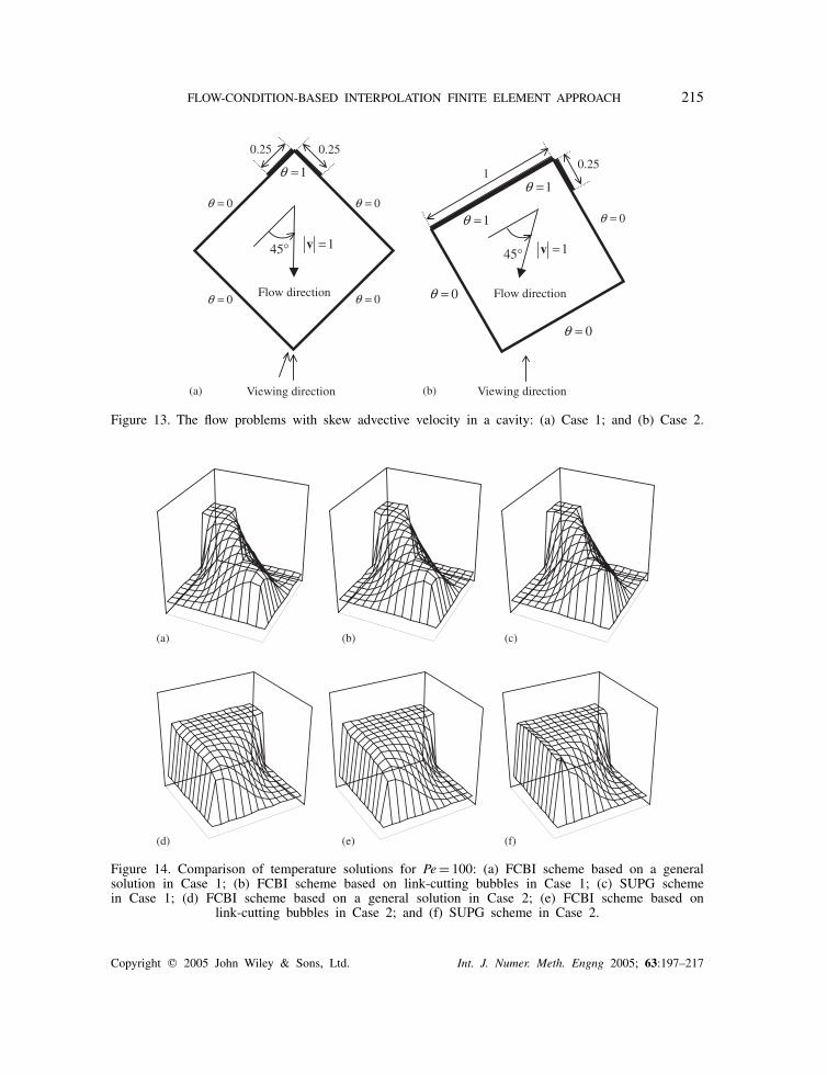
In the test problem of Section 4.1, the temperature is distributed rather smoothly in the y di-rection since the temperature boundary condition is given by a cosine function and the velocitycomponent in the y direction is zero. We consider next solutions that are more difficult to obtainwhen considering high Péclet number conditions due to the discontinuous temperature distri-butions and a skew advective velocity. The problems are defined in Figure 13. In this analysis,the Dirichlet boundary condition is imposed with the high temperature (� = 1) and the low tem-perature (� = 0). The 45◦ skew advective velocity, whose magnitude is 1, is prescribed over thewhole domain. Therefore, the problem becomes symmetrical with respect to the diagonal linein Case 1, while it is asymmetrical in Case 2. A rather coarse mesh of 12 × 12 square elementsis used for these flow problems, and this mesh is too coarse to reach an accurate solution usingthe original FCBI scheme when the Péclet number is high. While analytical solutions to the
Copyright � 2005 John Wiley & Sons, Ltd. Int. J. Numer. Meth. Engng 2005; 63:197–217
212 H. KOHNO AND K. J. BATHE
-0.50
-0.25
0.00
0.25
0.50
0.00 0.30 0.60 0.90
x
y
-0.50
-0.25
0.00
0.25
0.50
0.00 0.30 0.60 0.90
x
y
-0.50
-0.25
0.00
0.25
0.50
0.00 0.30 0.60 0.90
x
y
Exact solution Original FCBI
FCBI based on a general solution
FCBI based on link-cutting bubbles
Exact solution Original FCBI
FCBI based on a general solution
FCBI based on link-cutting bubbles
(a) (b)
(c)
Figure 9. Comparison of temperature profiles on vertical lines obtained with the regular mesh:(a) Pe = 10; (b) Pe = 100; and (c) Pe = 106.
problems for intermediate Péclet numbers are not available, of course the solutions for Pe = 106
are known.In this case, it is interesting to also obtain the solution using the SUPG scheme. The SUPG
formulation is given by the equation
∫�
(hi + k�
‖v‖2 v·∇hi
)v·∇hj d��j + 1
Pe
∫�
∇hi ·∇hj d��j = 0 (44)
with hi the usual isoparametric interpolation functions [16], and
k� = �
2PeF(�)
F (�) = coth( �
2
)− 2
�
Copyright � 2005 John Wiley & Sons, Ltd. Int. J. Numer. Meth. Engng 2005; 63:197–217
FLOW-CONDITION-BASED INTERPOLATION FINITE ELEMENT APPROACH 213
(a) (b)
(c) (d)
Figure 10. Comparison of temperature solutions obtained with the distorted mesh for Pe = 100:(a) exact solution; (b) original FCBI scheme; (c) FCBI scheme based on a general solution; and
(d) FCBI scheme based on link-cutting bubbles.
� = Pe√(
v̄�h�)2 + (v̄�h�
)2 (45)
where the subscripts i and j denote the global node numbers.The temperature solutions for Pe = 100 calculated with the two proposed FCBI and the
SUPG schemes are given in Figure 14. As shown, all the numerical results are similar and thetemperature distribution is symmetrical with respect to the diagonal line in Figures 14(a)–(c).The results obtained with the two FCBI schemes are more stable than those obtained with theSUPG scheme since unrealistic behaviour is seen close to the low temperature boundary inFigures 14(c) and (f).
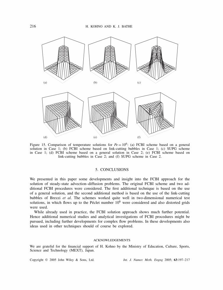
Figure 15 shows the temperature solutions for Pe = 106. In this case, the temperature changessharply, indeed discontinuously, on the boundary of the high temperature band due to the veryhigh Péclet number flow. In both cases, the results obtained with the proposed FCBI proce-dures can be considered accurate in contrast to the results obtained using the SUPG scheme.Of course, further studies of these problems with different meshes and boundary conditionsmight be pursued and would be valuable.
Copyright � 2005 John Wiley & Sons, Ltd. Int. J. Numer. Meth. Engng 2005; 63:197–217
214 H. KOHNO AND K. J. BATHE
(a) (b)
(c) (d)
Figure 11. Comparison of temperature solutions obtained with the distorted mesh for Pe = 106:(a) exact solution; (b) original FCBI scheme; (c) FCBI scheme based on a general solution; and
(d) FCBI scheme based on link-cutting bubbles.
0.0
0.2
0.4
0.6
0.8
1.0
1.2
0.0 0.2 0.4 0.6 0.8 1.0
x
θ Exact solution
Original FCBIFCBI based on a general solution
FCBI based on link-cutting bubbles
Figure 12. Comparison of temperature values on the centre line obtainedwith the distorted mesh for Pe = 106.
Copyright � 2005 John Wiley & Sons, Ltd. Int. J. Numer. Meth. Engng 2005; 63:197–217
FLOW-CONDITION-BASED INTERPOLATION FINITE ELEMENT APPROACH 215
(a) (b)
1=θ
0=θ
1=v°45
0.25
Flow direction 0=θ
0=θ
0=θ
0.25
Viewing direction
1=θ1
1=θ
1=v°45
0=θ
0=θ
0=θ
Flow direction
0.25
Viewing direction
Figure 13. The flow problems with skew advective velocity in a cavity: (a) Case 1; and (b) Case 2.
(a) (b) (c)
(d) (e) (f)
Figure 14. Comparison of temperature solutions for Pe = 100: (a) FCBI scheme based on a generalsolution in Case 1; (b) FCBI scheme based on link-cutting bubbles in Case 1; (c) SUPG schemein Case 1; (d) FCBI scheme based on a general solution in Case 2; (e) FCBI scheme based on
link-cutting bubbles in Case 2; and (f) SUPG scheme in Case 2.
Copyright � 2005 John Wiley & Sons, Ltd. Int. J. Numer. Meth. Engng 2005; 63:197–217
216 H. KOHNO AND K. J. BATHE
(a) (b) (c)
(d) (e) (f)
Figure 15. Comparison of temperature solutions for Pe = 106: (a) FCBI scheme based on a generalsolution in Case 1; (b) FCBI scheme based on link-cutting bubbles in Case 1; (c) SUPG schemein Case 1; (d) FCBI scheme based on a general solution in Case 2; (e) FCBI scheme based on
link-cutting bubbles in Case 2; and (f) SUPG scheme in Case 2.
5. CONCLUSIONS
We presented in this paper some developments and insight into the FCBI approach for thesolution of steady-state advection–diffusion problems. The original FCBI scheme and two ad-ditional FCBI procedures were considered. The first additional technique is based on the useof a general solution, and the second additional method is based on the use of the link-cuttingbubbles of Brezzi et al. The schemes worked quite well in two-dimensional numerical testsolutions, in which flows up to the Péclet number 106 were considered and also distorted gridswere used.
While already used in practice, the FCBI solution approach shows much further potential.Hence additional numerical studies and analytical investigations of FCBI procedures might bepursued, including further developments for complex flow problems. In these developments alsoideas used in other techniques should of course be explored.
ACKNOWLEDGEMENTS
We are grateful for the financial support of H. Kohno by the Ministry of Education, Culture, Sports,Science and Technology (MEXT), Japan.
Copyright � 2005 John Wiley & Sons, Ltd. Int. J. Numer. Meth. Engng 2005; 63:197–217
FLOW-CONDITION-BASED INTERPOLATION FINITE ELEMENT APPROACH 217
REFERENCES
1. Bathe KJ (ed.). Computational fluid and solid mechanics. Proceedings of the First MIT Conference onComputational Fluid and Solid Mechanics. Elsevier: Amsterdam, 2001.
2. Bathe KJ (ed.). Computational fluid and solid mechanics 2003. Proceedings of the Second MIT Conferenceon Computational Fluid and Solid Mechanics. Elsevier: Amsterdam, 2003.
3. Brooks AN, Hughes TJR. Streamline upwind/Petrov–Galerkin formulations for convection dominated flowswith particular emphasis on the incompressible Navier–Stokes equations. Computer Methods in AppliedMechanics and Engineering 1982; 32:199–259.
4. Hughes TJR, Franca LP, Hulbert GM. A new finite element formulation for computational fluid dynamics:VIII. The Galerkin/least-squares method for advective–diffusive equations. Computer Methods in AppliedMechanics and Engineering 1989; 73:173–189.
5. Franca LP, Frey SL. Stabilized finite element methods: II. The incompressible Navier–Stokes equations.Computer Methods in Applied Mechanics and Engineering 1992; 99:209–233.
6. Brezzi F, Russo A. Choosing bubbles for advection–diffusion problems. Mathematical Models and Methodsin Applied Sciences 1994; 4:571–587.
7. Zienkiewicz OC, Taylor RL. The Finite Element Method—Volume 3 Fluid Dynamics (5th edn). Butterworth-Heinemann: Stoneham, MA, 2000.
8. Bathe KJ, Pontaza JP. A flow-condition-based interpolation mixed finite element procedure for higher Reynoldsnumber fluid flows. Mathematical Models and Methods in Applied Sciences 2002; 12:525–539.
9. Bathe KJ, Zhang H. A flow-condition-based interpolation finite element procedure for incompressible fluidflows. Computers and Structures 2002; 80:1267–1277.
10. Bathe KJ, Zhang H. Finite element developments for general fluid flows with structural interactions.International Journal for Numerical Methods in Engineering 2004; 60:213–232.
11. Hendriana D, Bathe KJ. On upwind methods for parabolic finite elements in incompressible flows.International Journal for Numerical Methods in Engineering 2000; 47:317–340.
12. Grätsch T, Bathe KJ. Goal-oriented error estimation in the analysis of fluid flows with structural interactions,in preparation.
13. Yabe T. A universal numerical solver for solid, liquid and gas. In Proceedings of the First MIT Conferenceon Computational Fluid and Solid Mechanics, Bathe KJ (ed.). Elsevier: Amsterdam, 2003; 1424–1425.
14. Brezzi F, Hauke G, Marini LD, Sangalli G. Link-cutting bubbles for the stabilization of convection–diffusion–reaction problems. Mathematical Models and Methods in Applied Sciences 2003; 13:445–461.
15. Bathe KJ. The inf-sup condition and its evaluation for mixed finite element methods. Computers andStructures 2001; 79:243–252,971.
16. Bathe KJ. Finite Element Procedures. Prentice-Hall: Englewood Cliffs, NJ, 1996.
Copyright � 2005 John Wiley & Sons, Ltd. Int. J. Numer. Meth. Engng 2005; 63:197–217