1

Instrumentation IIMagnetometers and Calibration

2

Generic Space Instrument

Instrument

Analogue

SpacecraftInstrument

Digital

3

Sensor Technology Range (T) Suitable for space

SQUID 10-14 – 10 No – Cryostat needed

Optically Pumped 10-14 – 10-4 Yes – B and |B|

Fluxgate 10-10 – 10-4 Yes – B

Nuclear Precession 10-11 – 10-2 Yes - |B|

Hall Effect 10-3 – 10-2 No

Search Coil 10-12 – 106 Yes for AC fields

• Three B field components in range 0 - 30Hz• Wide measurement range 0.01nT – 50,000nT• Robust, reliable, high performance (low noise – stable offsets) • Optimised for power, mass, radiation etc.• Sensors fitted to a boom away from S/C magnetic disturbance

What do we mean by DC space magnetometer?

4

Optically Pumped Magnetometers • Heritage as a vector magnetometer • Vector and Scalar Operation (on Cassini)• Vector Mode

– RF discharge maintained in a He lamp – 1.08um– Creates radiation - channelled into a He absorption cell– He cell atoms are in meta-stable state also by RF discharge – Presence of ambient field causes Zeeman splitting– Emergent radiation is measured by IR detector– The measured absorption depends on efficiency of the optical pumping – Helmholtz coils around cell apply rotating sweep fields– Signal is obtained by measuring the modulation of rotating sweep fields

applied by surrounding Helmholtz coils– Results in a sinusoid whose magnitude and phase give the size and

direction of the field – Signal detected and fedback into the sensor coils

• Scalar mode – 1.08um radiation and frequency modulated AC field applied.– Absorption greatest when AC frequency = Larmor frequency. – Larmor frequency related to |B| by fundamental constants – Result is a very accurate measure of absolute field

Smith 1975

5

Proton Precession Magnetometers

• Proton rich material eg distilled water• Surrounded by induction coil • AC field induces proton precession • Once induced field switched off• Protons relax back to ambient field

precession • This induces a small AC signal in coil• Proportional to ambient field• Suitable for slow varying fields• Used for absolute measurement of B• Used on Earth mapping missions eg

Oested, CHAMP

Huggard 1970

6

FluxgateMGMs

Rotating coilMGMs

Search Coil MGMs

Induction Magnetometers

Faraday induction law →

)/)()(( Since /)(...

/

dttHtNAdVHBdtBAd

dtdV

roi

ro

i

μμμμ

===

Φ=

Expanded

dttHdNAdttHdANdttdHNA rororo /)( /)(/)(Vi μμμμμμ ++=

7

Anatomy of a Fluxgate• Operating Principle

– Soft permeable core driven around hysterisis loop– HEXT results in a net changing flux– Field proportional voltage induced in sense

winding– Closed loop improves linearity

• Advantages– Low noise ~ 20pT/ √Hz @1Hz– Wide dynamic range– Mature technology– Relatively inexpensive

• Disadvantages– Sensor mass– Sensor offset– Power ~ 1W– In-flight calibration overhead

8

HDVi 2f0

B

H

C1

C2HD

B

H

Drive (f0)

ΦCASE A: Zero external DC fieldHalf cores saturate synchronously – no net change of flux seen by sense wining

CASE B: Non-zero external DC fieldHalf cores do not saturate synchronously – a net change of flux seen by sense wining

Change of flux in sense winding at the 4 crossing of the B-H infection points in each drive period induced voltage at 2 x fo according to Faraday

CASE A

CASE B

9

Field magnitude determined by 2f magnitude

Field direction determined by 2f phase relative to reference

Reference 2f

Measured 2f

Fluxgate Control Electronics: Open Loop

10

Fluxgate Control Electronics: Closed Loop

Benefits include improved linearity and temperature stability. Scale factor depends only on feedback resistor/gain stage and coil constant.

Considerable effort spent minimising even harmonics in drive signal some odd harmonics due to transformer effect.

Includes anti-aliasing filter

11

Measured signal

Feedback signal

(Magnes 1999)

12

Equating terms and re-arranging

And if kSFLG2G1 >> 1

Two conclusionsMeasurement range only set by feedback circuit

Output noise is dominated by input amplifier and sensor noise only

(Very low noise analogue pre-amps available)

13

Fluxgate Noise

• Best expressed as a Noise Spectral Density (NSD) often at1Hz• Characteristic typically has a 1/f fall off

• Between 0 and Nyquist can use following expression to calculate RMS Noise

• Above Nyquist noise will be flat (ie white noise) due to ADC quantization

• Best quality fluxgates have NSD ~5pT/Root Hz at 1Hz

Ripka (1998)

14

Imperial fluxgate instrument performance– Industrial partner - Ultra Electronics– Cassini/Double Star Heritage– Two core sensor– Tuned second harmonic detection– Dual sense and feedback windings– Offset stability < 0.05 nT/°C – Scale factor drift < 40 ppm/°C – Noise density < 8pT/root Hz @1Hz – Operating range

• -80oC to 70oC (operational)• -130oC to 90oC (non-operational)

15

– Large number of bits N – Ideal linearity– No missing codes– Radiation tolerance– Ideal quantization noise

Importance of ADC: Quantization Noise

16

Quantization Noise – Large N Rad-tolerant ADCs are a ‘big’ problem for all instruments – Solution: MIL-STD devices with spot shields (N ~14)– Traditionally a separate self contained card – Cluster, Rosetta, Cassini – Use oversampling to reduce Q noise – Q noise should be matched to intrinsic sensor noise based on desired

range, resolution sensor scale factor and N and LSB

17

Digital Magnetometers – Means migrating control loop into digital domain – ADC and DAC utilised within sensor control loop – Offers increased flexibility - programmable– First Missions late 90s - ROMAP, VEX, Astrid, Oersted – Shown to reduce analogue content and power consumption– Numerous designs – still being played out - a very active field

Sensor core

Serial link to PC 22Hz

V to I converter

Sense winding

Drive winding

48kHzf (12kHz)

Drive circuitry

ADC48/96kHz(AD1835)

DAC6kHz

(AD1835)

ΣIntegrator

Field Correlation

(ADSP-21262)

ADSP 21262 Ex-Kit Eval. Board

A digital fluxgate control loop

18

Delta Sigma Fluxgates – A hot topic

– Single bit quantization at very high frequency– linear by definition– Tracks changes in consecutive samples rather than absolute value– ‘Ones’ density of the 1 bit data stream provides an average value of Vin– Can be implemented with a rad-hard analogue discretes and rad-hard

digital logic – mixed signal ASIC– Additional gain due to noise shaping– Eliminates need for old fashioned non rad-hard ADCs

19

Noise shaping effect

20

Delta-Sigma Magnetometer

O’Brien (2007)

Replace

+ + with

21

Anisotropic Magnetoresistance

• Magneto Resistance Effect– Change of resistance in magnetic field– AMR single layer permalloy, – AMR ΔR/Rmin of order 1- 2%– AMR has lowest noise floor – Johnson noise limited - no shot noise

• Barber Poles– Max, sensitivity & linearity at M v H 45o

– Conductive strips for linear operation

• AMR Sensors– Thin film solid state devices– Implemented as Wheatstone bridge– Mass <1g, Ceramic package – Sensitivity increases with increasing

bridge voltage, VB

( )( )Hθ2cos0ΔR0RR +=

Philips

22

Integrated coils

• Set - Reset Coils– Planar coils around each bridge resistor– Coil axis parallel to Easy axis– Used to re-align the anisotropic direction– Large current spike needed – Can extract sensor offset (unlike fluxgate)– Requires de-modulation to DC– Compensates for offset and offset drift– Improves sensor noise floor

• Offset coils – Integrated coils around the bridge– Coil axis parallel to Hard (sensitive) axis– Permits electromagnetic feedback– Used in closed loop back off measured field – Improves linearity and variation of sensitivity with

temperature– Suppresses Barkhausen noise

23

Single axis AMR magnetometer

• Analog build• Set-Rest 4A with 2μs τC

• Sensitivity proportional to VB

• Closed loop

COIL

FByo A

RHV ×=

24

Stimulus measurement – Fluxgate vs AMR

• Three layer Mu-Metal shield• 3Hz sine wave – 5nT ptp• Optimal AMR configuration• Closed loop, RFB=9kΩ• Bridge voltage 12V• Offset compensation• Flip frequency, 1.1kHz• Sensitivity ~ 11mV/nT• Sensitivity not linear with

increasing RFB

• Some residual offset in closed lop

• Temperature measurement outstanding

DSP (20mV/div scale)

AMR (20mV/div

scale)

25

Calibration equation for a vector magnetometer• Calibration Matrix 12 paramaters needed to transform measured volts to accurate

field components into a physically useful co-ordinate system eg GSE, GSM

– Calibration Matrix• Sensor gains – convert from raw volts to nT• Sensor mis-alignments – correct from deviation from nominal sensor axis• Euler angles –transform othogonalised components into required system

– Offset vector:• Sensor offset - correct for zero level readings (due to sensor, electronics or S/C)

– Calibration Files• Text files with calibration matrix & offset vector for each sensor on a daily or

orbit basis :

26

Imperial’s Magnetic Coil Facility

3 axis Helmholtz Coils

Sensor thermal chamber

Pit for long terms offset and noise measurement

27

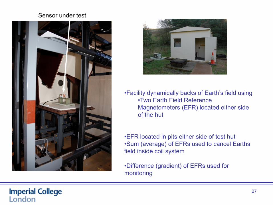
Sensor under test

•Facility dynamically backs of Earth’s field using•Two Earth Field Reference Magnetometers (EFR) located either side of the hut

•EFR located in pits either side of test hut•Sum (average) of EFRs used to cancel Earths field inside coil system

•Difference (gradient) of EFRs used for monitoring

28

Practical calibration models• Ground Calibration - we determine

– Sensor calibration parameters on ground,– Their associated temperature coefficients, – Their variations with input power– The sensor noise

• Magnetic Cleanliness Program - includes– Maximum length boom – Low field requirement at boom tip – Magnetic screening of materials and units– A spacecraft magnetic model– System level magnetic test

• In-flight – range switching, calibration steps– In-flight calibration techniques– Use of multiple sensors– Use of absolute and vector sensors– Use of dual-gradiometer modes

OB IB

29

System Level Magnetic Test: Cluster Example

Cluster had a very rigorous (and expensive) magnetic cleanliness program

A S/C magnetic field of < 0.25nT is almost NOT the case on the vast majority of S/C

30

In-flight calibration techniques• Spin stabalised spacecraft

– Fourier analysis on spinning data– Permits recovery of 8 of the 12 cal parameters– Major error – spin axis offset – Residual spin tone indicates calibration error– Example Missions:

• Cluster, Ulysses, Double Star, Equator-S, Themis

• Three-axis stabalised spacecraft– More difficult to calibrate – Utilise S/C rolls for offset measurement– Statistical analyses of solar wind data– Looks for correlations between B and B components– Additional absolute reference magnetometer useful– Example Missions

• Cassini, Rosetta, Oersted, Venus Express

• Multiple spacecraft missions = multiple calibration references

31

Multi-S/C Calibration – Cluster Example

Courtesy J. Gloag

32

Solution 2:p~ =+20cmm~=229mAm2

Bam~=9.6nT

Solution 1: p~ = - 20cmm~=594mA2

Bam~=6.31nT

Mod.dip. field

Obs. field

Real ambient field

Dual Magnetometer Mode – Used in cases where S/C field

contaminates measurement– IB and OB sensor used as a

gradiometer– Ambient field same at both IB & OB– S/C field NOT same at IB & OB– Number of sensors is proportional

to multipole moment that may be extracted

– Two sensors limit model to a dipole of fixed position

– Other techniques utilising pattern recognition in operation

– Relative sampling of both sensors important especially on spinning S/C

– Usually results in reduced data rates

– Example missions: Double Star, Venus Express

Example (1 dim.): Real Bam=10 nTReal SC dipole:

p =25 cmm =200 mAm2

Figure courtesy Delva

33

Case Study. Double Star magnetometer• OB sensor 5m, IB sensor 3.5m• Spin synchronised disturbance due to unbalanced solar array current• Amplitude varies with S/C shunting mode• Data cleaned using gradiometer mode • Resulting data set is spin averaged resolution (0.25Hz) compared to 11Hz on-board

Un-cleaned data and shunting modes Un-cleaned and cleaned data Carr (2005)

34

A new magnetometer model?

• Fluxgate - AMR combination • Single fluxgate at end of a (shorter boom) • Several AMR sensors inward of the fluxgate• Permits multipole expansion of S/C field• Accurate separation ambient field at instrument

intrinsic data rate• Precise tracking of fluxgate offsets• Required for space plasma constellations• Potential for automation• Could be applied acoss missions• Extendable to an array of AMR sensors

S/C

Fluxgatesensor

AMR sensors

Question – How to validate concept ?

Short boom

35

A magnetometer array• Imperial College student satellite program

– Milestone - Two spacecraft in LEO – 10cm cube, 1kg modules– Injection into LEO approx $30,000

• Aims– Measure ULF wave field in dayside

magnetosphere– Flight qualify FPGA controlled AMR array– Validate S/C field rejection algorithms– Extract accurate magnetic field vector

• Ground validation– Mobile Coil Facility– ESTEC MDM to calculate E-box moments– Measure both S/C components and

assembled S/C– Measured moments fitted to S/C model– Permits validation test of field rejection on

ground

Image courtesy of C. Howell

36

Potential Flight Opportunity 2010

• Collaboration between UCB, IC & NASA AMES• Space plasma science measurement on 3U CubeSat• Led by UCB/SSL• LEO with >65o inclination (72o nominal), 650km•1m deployable boom• Spin stabalised at ~1rpm• Two MAG sensors• Submitted to NSF Space Weather Competition 2008• To be re-submitted 2009• Heritage: GeneSat & STEREO

CINEMA- CubeSat for measurement of ions, neutrals and magnetic fields

37

Magnetometer1m boom

MAGIC Sensor head

MAGIC Magnetometer ModesAttitude ModeAccuracy <25nT, <150mWScience ModeAccuracy <2nT, <750mWInstrument Range +/-65536nTResolution: 0.25nT

CINEMA Magnetometer

MAG Boom Harness

1m extendable boom Boom mass ~120gMAG orientation not controlledDetermined by magneto-torquer pulse post deployment Following de-tumble CubeSat spun up and spin axis aligned normal to ecliptic