integrated models and methodologies for parameter …

The Pennsylvania State University

The Graduate School

Department of Industrial and Manufacturing Engineering

INTEGRATED MODELS AND METHODOLOGIES FOR PARAMETER AND

TOLERANCE DESIGNS

A Dissertation in

Industrial Engineering and Operations Research

by

Jawad S. Hassan

2012 Jawad S. Hassan

Submitted in Partial Fulfillment

of the Requirements

for the Degree of

Doctor of Philosophy

August 2012

ii

The dissertation of Jawad S. Hassan was reviewed and approved* by the following:

M. Jeya Chandra

Professor of Industrial and Manufacturing Engineering

Dissertation Advisor, Chair of Committee

Paul Griffin

Professor of Industrial and Manufacturing Engineering

Peter and Angela Dal Pezzo Department Head Chair

Tao Yao

Assistant Professor of Industrial and Manufacturing Engineering

David R. Hunter

Associate Professor of Statistics

*Signatures are on file in the Graduate School

iii

ABSTRACT

Most products are mixtures or assemblies of multiple components. These

components require determining the means (nominal values) and acceptable tolerances of

their relevant quality characteristics. The process of setting the means and tolerances of

the components characteristics is called parameter and tolerance designs. These designs

are found to be most effective when conducted simultaneously (integrated designs). In

the classical models of integrated parameter and tolerance designs, the objective is to

minimize the total costs while meeting the customer requirements and expectations using

available technological capabilities. Total costs can be divided into two categories. The

first category is the manufacturing costs, which include production and internal failure

costs, i.e. costs incurred before the product is shipped to the customer. The second

category is the quality losses or external failure costs, which include warranty costs, loss

of market share, etc., i.e. costs incurred after the product is shipped to the customer. The

major limitation of most existing integrated parameter and tolerance designs models is

the use of the quadratic loss function. It is used to capture all external failure costs

incurred by the manufacturer, customer, and the society as a whole as a function of the

deviation of the product’s quality characteristic from its ideal value using a single

proportionality constant. Despite the merits of its idea, the quadratic loss function suffers

from its simplistic form and the difficulty of estimating its proportionality constant.

In this research, integrated parameter and tolerance designs models are proposed

that use warranty costs instead of the quadratic loss function for estimating external

failure costs. The advantage of using warranty costs is that they are related to product

iv

reliability, which can be modeled fairly accurately using empirical product failure data.

However, since warranty costs are only part of the external failure costs, the first set of

proposed integrated models run the risk of underestimating the external failure costs and

jeopardizing the accuracy of the models results. This issue is addressed by proposing a

second set of integrated parameter and tolerance designs models, which incorporate in

them microeconomic and marketing concepts, such as pricing and demand functions. In

these integrated models, instead of listing and estimating all external failure costs other

than the warranty costs, these external failure costs are modeled as part of the customer’s

decision of the amount he or she is willing to pay for the product. That is, the customer

sets the purchase price based on a tradeoff between the amount of gained satisfaction and

the perceived risk of using the product. As a result, the objective of these integrated

models is to maximize the profit, which is the difference between the selling price and the

total cost of the product, as opposed to minimizing total cost. After surveying pricing and

demand models from the microeconomic and marketing literature, it is found that most

pricing models use product manufacturing and quality costs in a very crude manner.

Therefore, not only do the proposed integrated parameter and tolerance designs models

provide a better representation of the external failure costs, but they also provide a better

representation of manufacturing and quality costs of the product in the microeconomic

and marketing decisions models. That is, the proposed integrated models bridge the gap

between marketing and manufacturing operations and decisions by eliminating

unnecessary assumptions and poor links from both areas.

Several numerical examples are presented to validate the proposed models and

show their flexibility and applicability to a wide range of problems. For the first set of

v

integrated models, in which microeconomic and marketing decisions are not considered,

the examples include the cases of linear and nonlinear relationships between the

product’s main quality characteristic and the quality characteristics of its components as

well as the case of finite manufacturing processes. For the second set of integrated

models, in which microeconomic and marketing decisions are considered, the numerical

examples include the cases of static market analysis approach for a general demand

function, a monopoly, and a duopoly competition as well as the case of a dynamic market

analysis approach. In the different numerical examples, a variety of optimization and

analysis techniques, such as nonlinear programming, integer programming, response

surface methodology, simulation, and sensitivity analysis, are employed to show the

methodology of handling the different design problems.

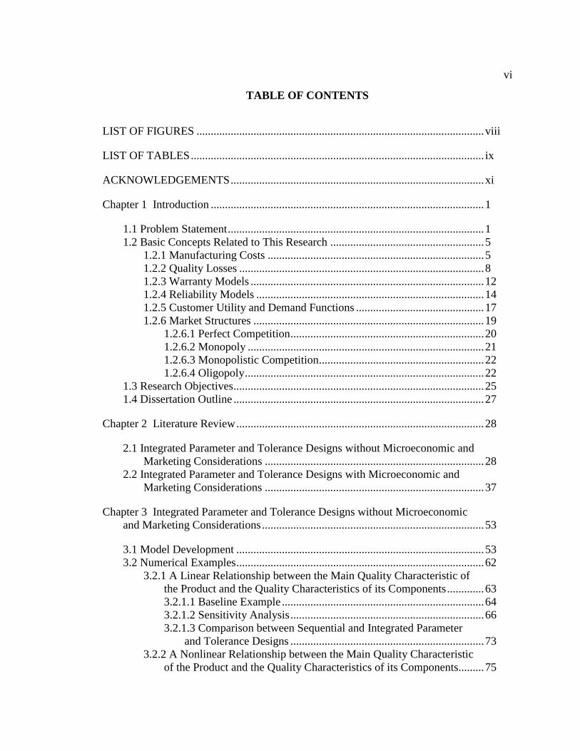
vi

TABLE OF CONTENTS

LIST OF FIGURES ..................................................................................................... viii

LIST OF TABLES ....................................................................................................... ix

ACKNOWLEDGEMENTS ......................................................................................... xi

Chapter 1 Introduction ................................................................................................ 1

1.1 Problem Statement .......................................................................................... 1

1.2 Basic Concepts Related to This Research ...................................................... 5 1.2.1 Manufacturing Costs ............................................................................ 5

1.2.2 Quality Losses ...................................................................................... 8 1.2.3 Warranty Models .................................................................................. 12

1.2.4 Reliability Models ................................................................................ 14 1.2.5 Customer Utility and Demand Functions ............................................. 17 1.2.6 Market Structures ................................................................................. 19

1.2.6.1 Perfect Competition .................................................................... 20 1.2.6.2 Monopoly ................................................................................... 21

1.2.6.3 Monopolistic Competition .......................................................... 22 1.2.6.4 Oligopoly .................................................................................... 22

1.3 Research Objectives ........................................................................................ 25

1.4 Dissertation Outline ........................................................................................ 27

Chapter 2 Literature Review ....................................................................................... 28

2.1 Integrated Parameter and Tolerance Designs without Microeconomic and

Marketing Considerations ............................................................................. 28

2.2 Integrated Parameter and Tolerance Designs with Microeconomic and

Marketing Considerations ............................................................................. 37

Chapter 3 Integrated Parameter and Tolerance Designs without Microeconomic

and Marketing Considerations .............................................................................. 53

3.1 Model Development ....................................................................................... 53 3.2 Numerical Examples ....................................................................................... 62

3.2.1 A Linear Relationship between the Main Quality Characteristic of

the Product and the Quality Characteristics of its Components ............. 63 3.2.1.1 Baseline Example ....................................................................... 64 3.2.1.2 Sensitivity Analysis .................................................................... 66 3.2.1.3 Comparison between Sequential and Integrated Parameter

and Tolerance Designs .................................................................... 73 3.2.2 A Nonlinear Relationship between the Main Quality Characteristic

of the Product and the Quality Characteristics of its Components......... 75

vii

3.2.2.1 Baseline Example ....................................................................... 76 3.2.2.2 Sensitivity Analysis .................................................................... 80

3.2.2.3 Comparison between Sequential and Integrated Parameter

and Tolerance Designs .................................................................... 84 3.2.3 Dealing with Discrete Tolerance-Costs Data Using Integer

Programming .......................................................................................... 86 3.3 Discussion ....................................................................................................... 89

Chapter 4 Integrated Parameter and Tolerance Designs with Microeconomic and

Marketing Considerations ..................................................................................... 92

4.1 Model Development ....................................................................................... 93

4.1.1 Example 1: Using a Demand Function to Capture Total Sales

during a Given Planning Horizon ........................................................... 98 4.1.2 Example 2: Using the Length of the Warranty Period and the

Process Capability Index as Signals for the Quality Level of the

Product ................................................................................................... 104

4.1.3 Example 3: A Duopoly Competition .................................................... 108 4.1.4 Example 4: A Dynamic Market Analysis Approach ............................ 112

4.2 Discussion ....................................................................................................... 115

Chapter 5 Research Contributions and Directions for Future Research ..................... 118

5.1 Research Contributions ................................................................................... 119

5.2 Directions for Future Research ....................................................................... 122

Appendix A Minitab Output of the Central Composite Design (CCD)...................... 124

Appendix B Cholesky Decomposition of a Two-by-Two Covariance Matrix ........... 126

Appendix C Normality Check for 1 2X X X ............................................................ 128

Bibliography ................................................................................................................ 131

viii

LIST OF FIGURES

Figure 1.1: Illustration of the phases of new product development. ............................ 2

Figure 2.1: Decisions and influences affecting product design. .................................. 38

Figure 3.1: Illustration of the stack-up constraint for t . a) The extreme case

where is as small as possible while maintaining , minpk actual pkC C , b) the

other extreme case where is as large as possible while maintaining

, minpk actual pkC C , c) a general case where , minpk actual pkC C . (Note: in the

figures, the distribution of the main product characteristic X is normal and

min 1pkC ). ............................................................................................................ 61

Figure 3.2: Illustration of the difference between the effect of varying pkC on the

optimal solution versus varying minpkC in the model. ........................................... 71

Figure 4.1: Illustration of the change in quantity demanded Q as a function of the

selling price P and the length of the warranty period w ( 2.5 and

0.3 ). ................................................................................................................ 99

Figure 4.2: Illustration of the change in selling price P as a function of the length

of the warranty period w and the process capability index pkC . ......................... 106

Figure C.1: Probability Density Functions (PDFs) of 1 2X X X and the normally

distributed X . ...................................................................................................... 129

Figure C.2: Normal probability plot for 1 2X X X . ................................................... 130

Figure C.3: Normal probability plot for the normally distributed X . ........................ 130

ix

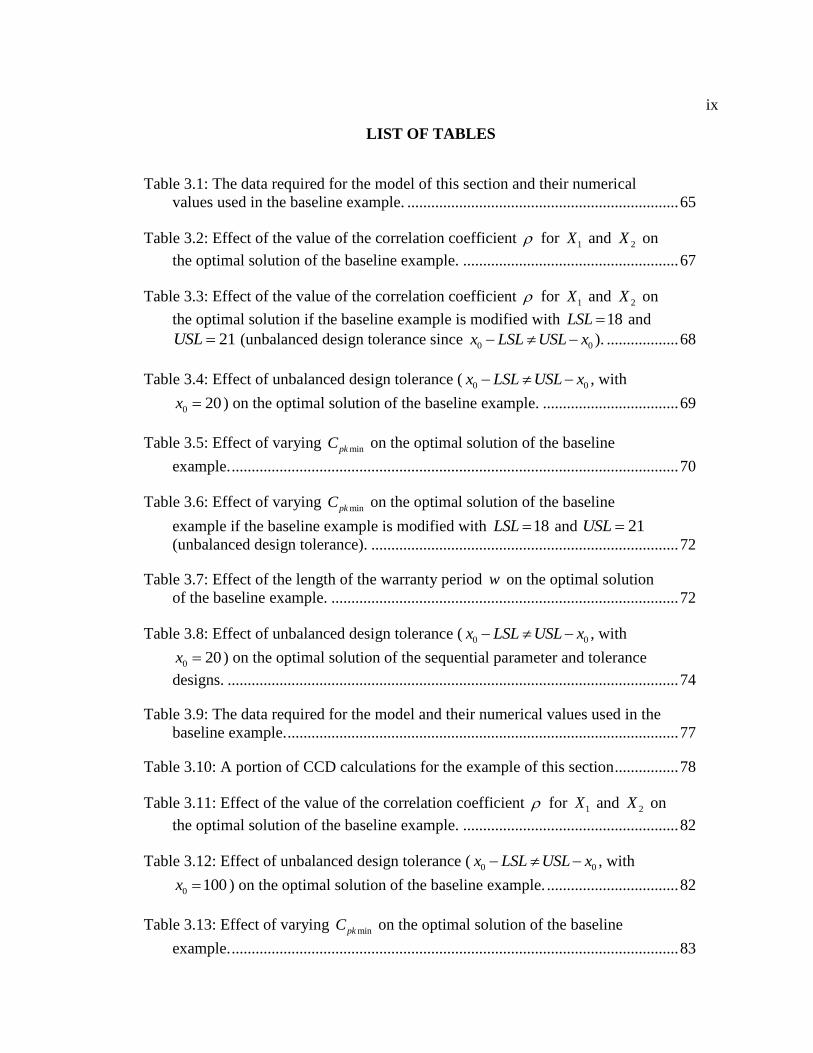
LIST OF TABLES

Table 3.1: The data required for the model of this section and their numerical

values used in the baseline example. .................................................................... 65

Table 3.2: Effect of the value of the correlation coefficient for 1X and 2X on

the optimal solution of the baseline example. ...................................................... 67


the optimal solution if the baseline example is modified with 18LSL and

21USL (unbalanced design tolerance since 0 0x LSL USL x ). .................. 68

Table 3.4: Effect of unbalanced design tolerance ( 0 0x LSL USL x , with

0 20x ) on the optimal solution of the baseline example. .................................. 69

Table 3.5: Effect of varying minpkC on the optimal solution of the baseline

example. ................................................................................................................ 70


example if the baseline example is modified with 18LSL and 21USL

(unbalanced design tolerance). ............................................................................. 72

Table 3.7: Effect of the length of the warranty period w on the optimal solution

of the baseline example. ....................................................................................... 72


0 20x ) on the optimal solution of the sequential parameter and tolerance

designs. ................................................................................................................. 74

Table 3.9: The data required for the model and their numerical values used in the

baseline example. .................................................................................................. 77

Table 3.10: A portion of CCD calculations for the example of this section ................ 78


the optimal solution of the baseline example. ...................................................... 82


0 100x ) on the optimal solution of the baseline example. ................................. 82


example. ................................................................................................................ 83

x

Table 3.14: Effect of the length of the warranty period w on the optimal solution

of the baseline example. ....................................................................................... 84

Table 3.15: Effect of the correlation coefficient on the optimal solution of the

sequential parameter and tolerance designs. ......................................................... 85


0 100x ) on the optimal solution of the sequential parameter and tolerance

designs. ................................................................................................................. 86

Table 3.17: Example of a tolerance-costs data list for the quality characteristics of

two components of a product. ............................................................................... 87

Table 4.1: The values of the model parameters and constraints that are common

among all the examples of the integrated models presented in this chapter. ........ 97

Table 4.2: The values of the model parameters and constraints that are specific to

the example of this section. .................................................................................. 100

Table 4.3: Effect of the selling price elasticity on the optimal solution. ................ 101

Table 4.4: Effect of the length of the warranty period elasticity on the optimal

solution. ................................................................................................................ 102







Table 4.8: The optimal solution for each of the ten half year periods. ........................ 115

xi

ACKNOWLEDGEMENTS

First of all, I would like to thank everyone who had a hand in the success of this

work and my years of education at Penn State. In particular, I would like to show my

gratitude to my advisor Dr. M. Jeya Chandra for his guidance, patience, and friendship. I

would also like to express my appreciation to my Ph.D. committee members: Dr. Paul

Griffin, Dr. Tao Yao, and Dr. David Hunter for their kindness, professionalism,

constructive comments, and valuable suggestions. I am forever grateful to the Penn State

community as a whole for being great hosts and giving me the best years of my life.

I would also like to thank all of my friends over the years in the United States for

making me feel right at home and my friends in Kuwait for staying as close of friends as

ever, even with the long years of separation.

I am forever indebted to my caring and loving parents and great brothers and

sisters. Their constant encouragement and prayers helped me through all the difficulties

and challenges of my life. I would like to specifically acknowledge my older brothers,

Sadeq and Dr. Mahdi, for the great impact they have had on my education and career.

There are no words that can describe my appreciation for my wife and her

unconditional love and support. I can only thank God Almighty, Allah, for blessing me

with her and with our two beautiful daughters, Mariam and Zainab.

Chapter 1

Introduction

1.1 Problem Statement

In today’s economy, fierce competition requires manufacturers to strive for

perfection and operate at the highest levels of efficiency when it comes to fulfilling and

exceeding customer requirements and expectations. This cannot be achieved without

taking full advantage of the enormous amounts of data collected about the marketplace

and customer behavior as well as the financial resources and technological capabilities of

the firm in making critical decisions about the products being manufactured. This

requires proper data analysis, model building and finding solutions while taking into

consideration every issue that could impact the success of the product.

The focus of this research is on parameter and tolerance designs, which are part of

the product design phase of new product development. The different phases of new

product development are presented in Figure 1.1.

2

Figure 1.1: Illustration of the phases of new product development.

Typically, new product lifecycle starts with surveying customer preferences and

market information (Park et al., 2008). Then, product design and process design are

conducted. After that, actual production, sales, and after-sales services follow. It is

important to emphasize that not only does product design highly depend on the

information collected about the marketplace and customer preferences, but it also greatly

influences the later phases of process design, production, sales, and after-sales services.

Thus, the key idea is that, even though the actual implementation of the different phases

of new product development occurs sequentially, the decision making process and the

mathematical models used in product design ought to encompass all the information

related to customer preferences, market structure, selling price, manufacturing

capabilities and costs, product reliability, and warranty costs as well as any other

information that could contribute to the success and profitability of the product. This idea

is the main premise of this research.

Surveying Customer

Preferences and

Market Information

Product Design

• System Design

• Parameter Design

• Tolerance Design

Process Design

• System Design

• Parameter Design

• Tolerance Design

Production Sales After-Sales Services

3

As shown in Figure 1.1, product design consists of three main steps that are

conventionally followed in sequence as advocated by Dr. Genichi Taguchi (Park et al.,

2008). These three steps of product design are system design, parameter design, and

tolerance design. System design is the process of developing a prototype of the product

detailing its features, components, assembly, functionality, etc. Parameter design is the

process of determining the means (nominal values) for all the quality characteristics of

the components of the final product, which are typically optimized to achieve the

functional requirements of the product with the least variability and maximum robustness

against uncontrollable noise factors. Tolerance design is the final process of assigning

tolerances to the quality characteristics of the product and its components with the

objective of minimizing manufacturing costs in order to further reduce the variability, if

the variability could not be satisfactorily minimized by parameter design (Chandra,

2001). It is worth mentioning that process design also consists of the same three steps of

system design, parameter design, and tolerance design. In system design, the

manufacturing process with all the steps required for production is developed based on

available resources and technologies. In parameter design, the operating conditions and

machine settings for the product manufacturing process are determined. Lastly, in

tolerance design, tolerances are assigned to the manufacturing process conditions and

settings (Park et al., 2008).

In the product design phase, the sequential application of system design,

parameter design, and tolerance design has been criticized as being suboptimal. For

instance, there are several studies that argue that adjusting the tolerances of the

components characteristics in tolerance design after their mean values have been set in

4

parameter design could affect the optimality of these mean values (e.g., Li et al., 1999;

Jeang, 1999; Cho et al., 2000; etc.). These studies focus on the integration of parameter

and tolerance designs with the objective of minimizing costs. That is, it is suggested that

parameter and tolerance designs ought to be conducted simultaneously in order to achieve

an optimal design. Furthermore, there are other studies that argue that an integrated

approach, which utilizes all the information related to the manufacturing and marketing

operations during product development, would result in a more profitable outcome for the

firm (e.g., Bagajewicz, 2005; Karmarkar et al., 1997; etc.). Often, a product is

manufactured based on what is best or optimal from the point of view of the

manufacturer and then the marketing team is asked to try and sell the product

(Bagajewicz, 2005). Other times, a product is designed with all the functional

requirements, parameters and tolerances based on market information and what the

customer wants, while manufacturing process selection and costs involved are ignored.

These practices can either result in unnecessary costs and wasted resources with little

return on investment or they can result in lost opportunities and the failure to meet

expectations. Thus, it seems more logical to include marketing decisions and the voice of

the customer in all the stages of product development along with full consideration of the

manufacturing capabilities and costs in order to achieve maximum efficiency and

profitability.

The only downside of such approaches, which call for more holistic

methodologies for the implementation of product design, is the added complexity of the

models and the difficulty to solve them. Then again, with the rapid improvements in the

technological and computer capacities, optimization algorithms, data mining, etc., solving

5

massive numerical problems and complex models can be performed more easily today

than ever before.

The problem with previous studies that attempt to provide integrated models for

parameter and tolerance designs (or product development in general), as presented in

more detail in the literature review of Chapter 2, is that there tends to be an emphasis by

some studies on manufacturing issues while having a very simplistic treatment of

marketing issues. On the other hand, there are other studies that have the exact opposite

problem where there tends to be an emphasis on marketing issues while crudely

representing manufacturing issues. Therefore, the main contribution of this research is to

propose integrated parameter and tolerance designs models that emphasize the

importance of both manufacturing and marketing issues. However, before presenting the

detailed objectives of this research in section 1.3, a brief description of the basic concepts

related to the proposed models in this research is presented. These basic concepts include

manufacturing costs, quality losses, warranty models, reliability models, customer utility

and demand functions, and market structure types.

1.2 Basic Concepts Related to This Research

1.2.1 Manufacturing Costs

In manufacturing and quality engineering literatures, manufacturing costs are

typically modeled as a function of the natural process tolerances of the quality

characteristics of the product components. The tighter the tolerances, the higher the

6

manufacturing costs and vice versa. This is because it takes more effort and perhaps

slower production rate as well as more skilled workers, more expensive production and

monitoring equipments with high precision, etc., in order to maintain tighter tolerances

(Jeang, 2001). The relationship between manufacturing costs and the natural process

tolerances of the components characteristics could be presented in the form of a

tolerance-cost table, which lists the level of tolerance and the cost associated with it (Li et

al., 1999), or it could be presented in functional form using, for instance, the reciprocal or

the exponential relationships given by (Wu et al., 1998):

2

0 1

dMC d d t

(1.1)

and

0 1 2expMC d d td (1.2)

respectively, where t is the natural process tolerance of the component characteristic and

0d , 1d and 2d are model parameters. These formulations are typical in the literature and

many studies define manufacturing costs only as a function of the natural process

tolerances of the components characteristics. However, there are other studies (e.g. Jeang,

2003) that include a separate internal failure costs term, i.e. scrap and rework costs, in

addition to the tolerance costs in the manufacturing costs relationship since they are

affected by the means as well as the natural process tolerances of the components

characteristics. If the mean of the main quality characteristic of the product is set at the

midpoint within the allowable design tolerance or very close to it, then the internal failure

costs could be modeled as a function of the natural process tolerances of the components

characteristics alone and lumped into the tolerance-cost relationships mentioned above

7

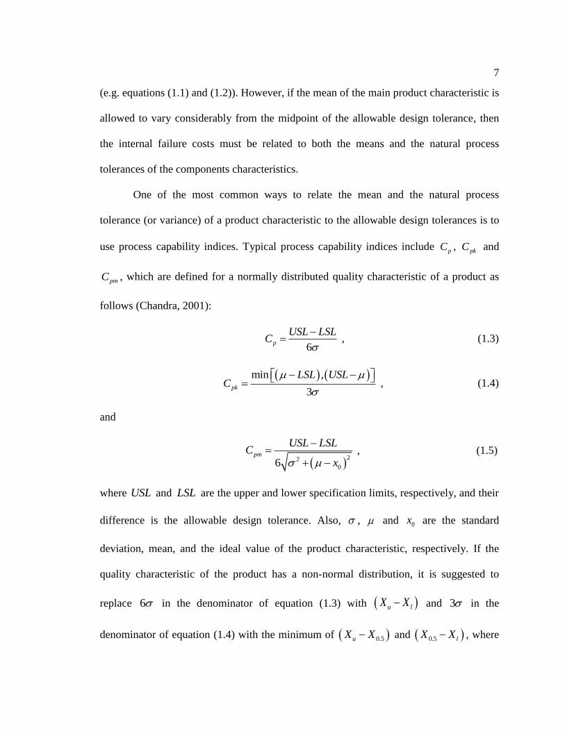
(e.g. equations (1.1) and (1.2)). However, if the mean of the main product characteristic is

allowed to vary considerably from the midpoint of the allowable design tolerance, then

the internal failure costs must be related to both the means and the natural process

tolerances of the components characteristics.

One of the most common ways to relate the mean and the natural process

tolerance (or variance) of a product characteristic to the allowable design tolerances is to

use process capability indices. Typical process capability indices include pC ,

pkC and

pmC , which are defined for a normally distributed quality characteristic of a product as

follows (Chandra, 2001):

6

p

USL LSLC

, (1.3)

min ,

3pk

LSL USLC

, (1.4)

and

22

06pm

USL LSLC

x

, (1.5)

where USL and LSL are the upper and lower specification limits, respectively, and their

difference is the allowable design tolerance. Also, , and 0x are the standard

deviation, mean, and the ideal value of the product characteristic, respectively. If the

quality characteristic of the product has a non-normal distribution, it is suggested to

replace 6 in the denominator of equation (1.3) with u lX X and 3 in the

denominator of equation (1.4) with the minimum of 0.5uX X and 0.5 lX X , where

8

pX is the 100p percentile of the product characteristic and values for u and l include

1 and 0 , 0.99865 and 0.00135 , or 0.995 and 0.005 (Chandra, 2001; Clements, 1989;

and McCormack et al., 2000). It is worth mentioning that six-sigma companies require

their process capability indices to be around two.

In microeconomic and marketing literatures, on the other hand, manufacturing

costs, in general, are not related to the means and the natural process tolerances of the

product or components characteristics as in the manufacturing and quality engineering

literatures. Instead, manufacturing costs are either modeled as a function of some

attribute, such as quality level (Teng et al., 1996), product reliability (Huang, et al.,

2007), etc., or defined as the sum of fixed and variable costs (Miller, 2006). Here, fixed

costs are the costs that are independent of the production rate, which include costs related

to investment costs in facilities, heavy machinery, etc. Conversely, variable costs are the

costs that depend on the production rate, which include the costs of raw materials,

personnel, electricity, etc.

1.2.2 Quality Losses

In quality engineering literature, the most widely used formulation for estimating

the quality losses (external failure costs) is the quadratic loss function, which was first

developed by Dr. Taguchi. It is arrived at by employing the Taylor series expansion and

ignoring higher order terms. The final form of the quadratic loss function for a nominal-

the-best (N-type) quality characteristic X of a product is given by (Chandra, 2001):

2

0( ) ( ) ,L X k X x LSL X USL (1.6)

9

where k is a constant that represents the monetary loss incurred by the society after the

product is shipped due to a unit deviation of the product characteristic from its ideal value

0x . Also, LSL and USL are the lower and upper specification limits of the product

characteristic, respectively. The quadratic loss function states that quality losses increase

(quadratically) as the difference between the value of the product characteristic and its

ideal value increases, while there are no losses incurred if the value of the product

characteristic is equal to its ideal value. The main advantage for the use of the quadratic

loss function is this ability to capture the effect of the product characteristic deviation

from its ideal value in monetary value. The result is that any deviation from the ideal

value incurs losses, even if the product meets all the specifications and tolerances. This is

a big improvement over the “goal-post mentality” that assumes all products that meet the

specifications are identical in terms of quality (Chandra, 2001).

The expected value of the quadratic loss function (equation (1.6)) is given by:

2 2

0( ) ( )E L X k x (1.7)

where and 2 are the mean and variance of the product characteristic X . One of the

most significant and practical results of equation (1.7) is that the expected quality losses

are directly proportional to the variance and the deviation of the mean from the ideal

value of the product characteristic. Thus, the quadratic loss function suggests that setting

the mean equal to the ideal value and minimizing variability of the product characteristic

should be the goal of any manufacturing process in order to achieve high quality

products. That is, for a product with one main quality characteristic X that is a function

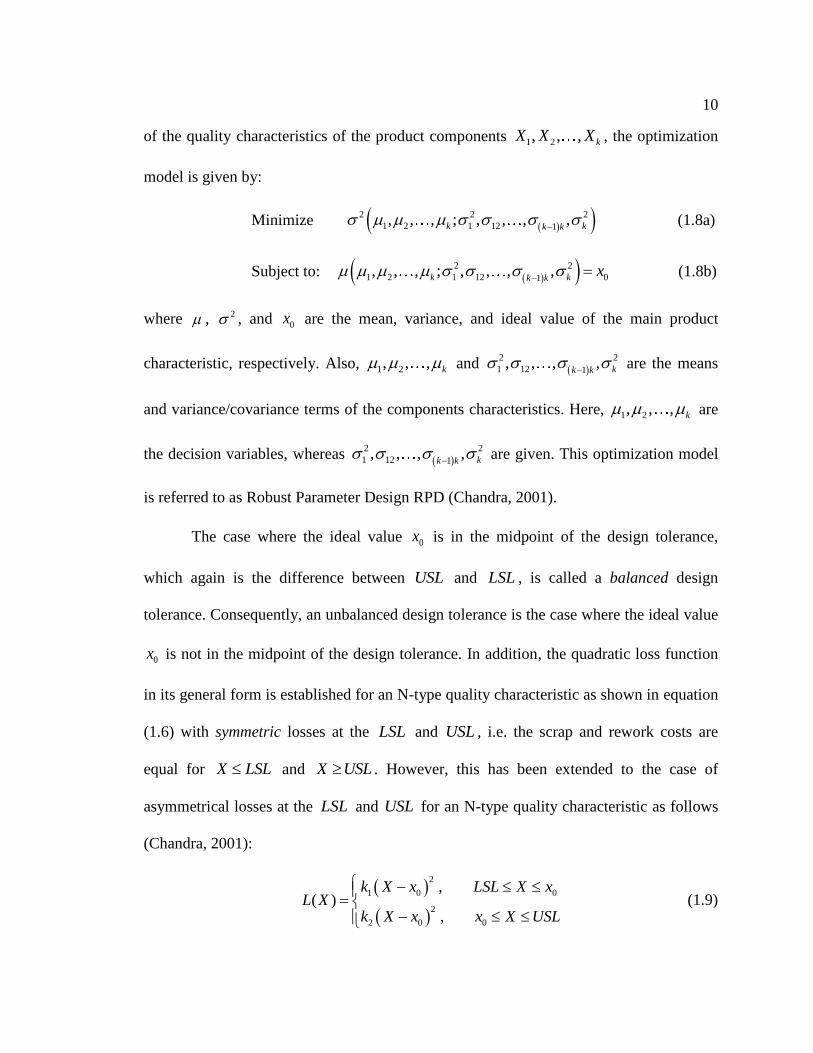
10

of the quality characteristics of the product components 1 2, , , kX X X , the optimization

model is given by:

Minimize 2 2 2

1 2 1 12 1, , , ; , , , ,k kk k

(1.8a)

Subject to: 2 2

1 2 1 12 01, , , ; , , , ,k kk k

x

(1.8b)

where , 2 , and 0x are the mean, variance, and ideal value of the main product

characteristic, respectively. Also, 1 2, , , k and 2 2

1 12 1, , , , kk k

are the means

and variance/covariance terms of the components characteristics. Here, 1 2, , , k are

the decision variables, whereas 2 2

1 12 1, , , , kk k

are given. This optimization model

is referred to as Robust Parameter Design RPD (Chandra, 2001).

The case where the ideal value 0x is in the midpoint of the design tolerance,

which again is the difference between USL and LSL , is called a balanced design

tolerance. Consequently, an unbalanced design tolerance is the case where the ideal value

0x is not in the midpoint of the design tolerance. In addition, the quadratic loss function

in its general form is established for an N-type quality characteristic as shown in equation

(1.6) with symmetric losses at the LSL and USL , i.e. the scrap and rework costs are

equal for X LSL and X USL . However, this has been extended to the case of

asymmetrical losses at the LSL and USL for an N-type quality characteristic as follows

(Chandra, 2001):

2

1 0 0

2

2 0 0

,( )

,

k X x LSL X xL X

k X x x X USL

(1.9)

11

where 1k and 2k are the monetary values of the loss to society for a unit deviation either

below or above the ideal value 0x , respectively. The cases of a smaller-the-better (S-type)

and larger-the-better (L-type) quality characteristics are also considered. For these cases,

the quadratic loss functions are given, respectively, by (Chandra, 2001):

2( ) ,L X k X X USL (1.10)

and

2

( ) ,k

L X X LSLX

(1.11)

The main limitation of the quadratic loss function is that it tries to lump all costs

associated with the deviation of the product from its ideal value into a single vaguely

defined parameter. The proportionality constant k of the quadratic loss function is

supposed to capture the loss to society as a whole due to the imperfection of the product

in monetary value. This loss could mean the liability and warranty costs incurred by the

manufacturer, the inconvenience and waste of time that the customer is faced with when

having to fix or replace the product, loss of future sales and the decline in the market

share of the firm, any environmental or unforeseen problems, lawsuits, etc. (Hassan,

2009). As it can be seen, even if it was possible to list all possible losses to society,

similar to those mentioned and others, putting a dollar value on each of these losses is

practically impossible in most cases. Moreover, these losses tend to be related to many

factors that could be interdependent. Thus, lumping all these losses into a single

parameter k is too simplistic and restrictive.

To Dr. Taguchi’s credit, however, it is mentioned in Taguchi et al. (1990) that the

quadratic loss function (QLF) “is a simple approximation, to be sure, not a law of

12

nature”. The authors continue to say that “actual field data cannot be expected to

vindicate QLF precisely, and if your corporation has a more exacting way of tracking the

costs of product failure, use it” (Taguchi et al., 1990).

Despite the limitations of the quadratic loss function, it is still widely used in the

literature perhaps for no reason other than not having a practical replacement.

It is worth mentioning that the quadratic loss function focuses on conformance

quality, whereas many microeconomic and marketing studies focus on performance

quality (Karmarkar et al., 1997). Thus, in the microeconomic and marketing literatures,

quality levels are commonly defined based on ordinal scales. For instance, the quality

levels are defined as grades or classes, i.e., grade A, grade B; class 1, class 2; etc. (Teng

et al., 1996), or other more descriptive classifications, such as worse than average,

average, better than average, etc. (Menezes et al., 1992). Then, quality losses are

estimated in relation to the defined quality levels.

1.2.3 Warranty Models

Generally, a warranty can be defined as “a contract or an agreement under which

the manufacturer of a product or service must agree to repair, replace, or provide service

when the product fails or the service does not meet the customer’s requirements before a

specified time (length of warranty)” (Elsayed, 1996). Thus, depending on the type of the

product and the type of service desired by the customer, manufacturers could offer a wide

range of warranty policies. To the customer, the warranty policy can serve as a signal for

the quality of the product in addition to the obvious purpose of protection against faulty

13

products. To the manufacturer, the warranty policy can be used as an advertising tool as

well as protection against the customer’s misuse of the product by providing clear

guidelines and detailed rights and responsibilities for both the customer and the

manufacturer (Monga et al., 1998).

Warranty policies could be for a finite period of time or lifetime warranties; they

could require the manufacturer to repair, replace, or provide a pro-rated or a lump-sum

rebate; or they could be a combination of the simpler warranty policies with specific rules

and requirements. Moreover, besides specifying the type of warranty policy to offer to

the customer, the manufacturer has to decide the length of the warranty period and the

cost of the warranty as well (Elsayed, 1996). Despite the fact that there are various types

of warranty models, only one simple warranty model, which is called the minimal repair

warranty model, is considered in this research to show how warranty models are

implemented in the proposed models. Other warranty models, which can be found in

Elsayed (1996) and Blichke et al. (1996), can be implemented in a similar manner. More

recent advances on the topic of warranty and its relation to reliability can be found in

Murthy (2006).

The minimal repair warranty model considered in this research was first

developed by Barlow et al. (1960). In this model, “it is assumed that the failure rate of the

product remains unchanged after a repair” (Nguyen et al. (1984)). This is typically the

case for a minor repair, which brings the system back to its original condition just before

the failure, or the replacement of a component that is a small part of a larger system such

that the reliability of the system remains practically unchanged due to the degradation of

its other components.

14

For the minimal repair warranty model, the expected number of failures during

the warranty period 0, w is given by (Nguyen et al. (1984)):

0

ln

w

M w h d R w (1.12)

where h is the hazard rate function and R w is the reliability at the end of the

warranty period w . Thus, the total warranty costs WC can be found by:

lnr rWC C M w C R w (1.13)

where rC is the expected repair cost per failure.

1.2.4 Reliability Models

A formal definition of reliability is given by Leemis (2009) and it states that “the

reliability of an item is the probability that it will adequately perform its specified

purpose for a specified period of time under specified environmental conditions”. Thus, it

follows from the definition that the main random variable of traditional reliability models

is time to failure . However, other random variables or parameters can also be included

in the reliability models resulting in reliability models with covariates. The studies by

Deleveaux (1997), Blue (2001), Zhang (2006) and Hassan (2009) try to relate the mean

and variance of the main quality characteristic of the product to warranty costs through

the use of reliability models with covariates. The reliability models that are considered in

this research are the ones developed by Blue (2001) and Hassan (2009), which are based

15

on the Weibull lifetime distribution. The conditional reliability for a product with a single

main N-type quality characteristic is given by (Blue, 2001):

2

0( | ) exp c

NR x a b x x

(1.14)

where a , b , and c are model parameters, x and 0x are the observed and ideal values of

the product characteristic, respectively, and is the time to failure. It is to be noted that

the model parameters, i.e. a , b , and c , are all nonnegative. The parameter a , when

0a , captures the rate at which the reliability of an item with an observed product

characteristic that is equal to the ideal value, i.e. 0x x , decreases over time. However,

when 0a and 0x x , the reliability is equal to one at all times, which means that the

item never fails. This situation is very unlikely especially for consumer products, where

used items tend to be less reliable than new items. Thus, the parameter a provides the

flexibility in the model to capture the wear of an item over time, even if its quality

characteristic equals the ideal value. In contrast, the quadratic loss function assumes the

external failure costs of an item with a product characteristic that is equal to its ideal

value is zero. The parameter b captures the intensity at which the reliability is penalized

for deviating from the ideal value. Lastly, the parameter c is a scaling parameter for the

time used in the model.

Analogous to the asymmetrical loss function case of an N-type quality

characteristic (equation (1.9)), if experience or life testing shows that the reliability is

affected differently when the value of the product characteristic is greater than its ideal

value 0x compared to when it is smaller than 0x , then an asymmetric conditional

16

reliability function can be used. That is, for an N-type product characteristic, the

asymmetric conditional reliability function is given by:

1

2

2

1 1 0 0

2

2 2 0 0

exp ,

( | )

exp ,

c

Nc

a b x x x x

R x

a b x x x x

(1.15)

where 1a , 1b , 1c , 2a , 2b , and 2c are model parameters, x and 0x are the observed and

ideal values of the product characteristic, respectively, and is the time to failure.

Moreover, similar to equation (1.14), the conditional reliabilities for S-type and L-type

product characteristics, respectively, are given by (Hassan, 2009):

2( | ) exp c

SR x a bx

(1.16)

and

2

( | ) exp c

L

bR x a

x

(1.17)

The unconditional reliabilities for normally distributed N-type and S-type product

characteristics, respectively, are given by (Blue, 2001; Hassan, 2009):

2

0

22

1exp

1 21 2

c

N cc

b xR a

bb

(1.18)

and

2

22

1exp

1 21 2

c

S cc

bR a

bb

(1.19)

17

where and 2 are the mean and variance of the product characteristic X . As for the

normally distributed L-type product characteristic X , the unconditional reliability can be

approximated by:

2

22

44

1

1exp

1 21 2

c

L

cc

b

R a

bb

(1.20)

The approximation in equation (1.20) is fairly accurate ( 5% error) for the case

when the ratio is large ( 10 ) (Hassan, 2009). This result is evident from a

Taylor series expansion of 1 X around , which is given by:

2

2 3

1 1 1 1X X

X

Remainder (1.21)

where the second- and higher-order terms in equation (1.21) can often be neglected when

the ratio is large. For example, the second-order term in equation (1.21) is simply a

chi-squared random variable with one degree of freedom divided by 2

. This

means that 1 X can be approximated with a first-order Taylor series expansion, which

results in the distribution of 1 X to be approximately normal with mean 1 and

variance 2 4 .

1.2.5 Customer Utility and Demand Functions

The level of customer satisfaction with respect to product attributes and price can

be captured by the customer’s utility function, where customer utility simply means

18

customer satisfaction. Even though customer utility can be a highly subjective concept

and differs from one customer to another, customer utility functions can still be useful in

capturing customer satisfaction trends and reactions to variations in product price and

attributes (Miller, 2006). One of the major phenomena that the concept of customer

utility is based upon is the law of diminishing marginal utility, where marginal utility

refers to the satisfaction a customer achieves from consuming an additional unit of the

product or commodity. The law of diminishing marginal utility states that “as an

individual consumes more of a particular commodity, the total level of utility or

satisfaction derived from that consumption usually increases. Eventually, however, the

rate at which it increases diminishes as more is consumed” (Miller, 2006).

The key idea that is relevant to this research is that customer utility functions can

be used as a measure of customer satisfaction relative to variations in product price and

quality. An intuitive relationship between customer satisfaction, on one hand, and product

price and quality, on the other, is that as the product price decreases and its quality

increases, customer satisfaction increases. In addition, the idea presented by the law of

diminishing marginal utility suggests that as the quality increases, the rate at which

customer satisfaction increases drops and, at some point, the customer would be willing

to pay less and less for further increases in quality. For instance, it is logical to say that

increasing the reliability of a refrigerator such that its useful life is improved from 7 to 17

years is more satisfying to the customer than improving the useful life from 25 to 35

years or, perhaps less realistically, from 40 to 50 years, even though the improvement in

useful life is ten years for all cases.

19

Alternatively, demand functions can be used to serve a similar purpose as the

customer utility functions. Since demand is directly affected by customer preferences and

utility, demand functions can be related to product price and quality to represent customer

and market behaviors. In this research, both customer utility and demand functions are

used to model the effects of price and quality on customer or market behaviors.

It is worth mentioning that, in elementary microeconomics, the relationship

between price and quantity demanded is commonly represented by a demand curve.

When there is a change in price only, the quantity demanded changes based on the

demand curve, i.e. moving along the demand curve. However, when there is a change in

factors other than price, such as customer preferences, product quality, market size, etc.,

the whole demand curve shifts (Miller, 2006). Demand curves are nothing but graphical

representations of demand functions.

1.2.6 Market Structures

In economic theory, there are several types of market structures. A monopoly, a

monopolistic competition, an oligopoly, and a perfect competition are examples of the

types of market structures. Pure monopoly and perfect competition market structures are

idealistic cases and fairly rare in real life. That is why “the vast majority of firms in

modern economies are either oligopolistic firms or monopolistic competitors” (Friedman,

1983). However, for completeness, the four types of market structure and their

characteristics are discussed briefly in this section. It is important to appreciate the

complex relationships among product price, demand, and quality as well as other factors

20

and dynamics in a given market structure in addition to the discrepancies across the

different types of market structures. Market structures and their characteristics can be

found in almost any microeconomic book (e.g. Miller, 2006; Boyes et al., 2011; etc.).

1.2.6.1 Perfect Competition

The perfect competition market structure has the following characteristics:

1. The numbers of producers and buyers are large.

2. The products are identical (homogenous), i.e. the quality is set.

3. Entering and exiting the market is easy.

4. Producers are price takers, i.e. the price is set.

5. The demand curve is horizontal, i.e. perfect demand elasticity.

6. Advertisement is not used, in general, since there is no product

differentiation.

7. Any quantity produced can be sold at the market price.

In perfect competition, the price and quality level of the product are set by the

market since individual producers constitute a very small portion of the market such that

their individual effects on market price and quality level are negligible. Thus, the task for

the producer is to determine the quantity of product to produce while minimizing cost,

subject to achieving a product that has a quality level that is commonly accepted or

expected in the market. This decision about the quantity of the product is made

independently from other producers’ decisions since the number of producers in the

21

market is large. Here, it is assumed that the customer has perfect knowledge and clear

expectation of the quality of the product that is to be purchased at the market set price.

Again, it is unlikely to find a market in real life that possesses all the characteristics of a

perfect competition market. However, well-established products, such as wheat and milk,

could be examples of a market that is close to a perfect competition.

1.2.6.2 Monopoly

The monopoly market structure has the following characteristics:

1. There is a single producer.

2. The product has no close substitute.

3. Entering the market is extremely difficult.

4. The demand curve is downward sloping but not perfectly inelastic.

A monopoly can be established and maintained when there is a huge barrier of

entry in the market by competitors. Barriers of entry include government regulations,

patents, economies of scale, high initial fixed costs, ownership of a rare resource, etc.

(Miller, 2006). Unlike a perfect competitor, whose main decision is the optimal output

level, a monopolist needs to simultaneously determine both the optimal selling price and

the optimal output level in order to maximize profit.

22

1.2.6.3 Monopolistic Competition

The monopolistic competition market structure has the following characteristics:

1. The numbers of producers and buyers are large.

2. The products offered in the market are differentiated (heterogeneous) but

they are close substitutes of each other.

3. Entering and exiting the market is relatively easy.

4. The demand curve is downward sloping but it is not as steep as that in a

monopoly.

5. Advertisement is used since there is product differentiation.

Since the demand curve is downward sloping, a monopolistically competitive

firm has some control over pricing unlike a perfectly competitive firm, which is a price

taker. However, this control over pricing does not reach the level of control enjoyed by a

monopolist. Moreover, similar to the perfect competition market structure, since there are

many producers in the market and entry into the market is relatively easy, decisions about

pricing and output level are made independently from other producers’ decisions and

reactions.

1.2.6.4 Oligopoly

The oligopoly market structure has the following characteristics:

1. The number of producers is small but the number of buyers is large.

23

2. Producers’ price, quantity and quality decisions in the market are

interdependent.

3. The products offered in the market could be identical or differentiated.

4. Entering and exiting the market is fairly difficult.

5. The demand curve is downward sloping and it can exhibit a discontinuity

(kinked demand curve).

6. Advertisement is used in the case of differentiated products.

In this market structure, since the whole market is composed of a few competitive

producers, decisions about product price, quality, quantity, etc., are made by each

producer while considering not only what is best for their firms, but also how the other

competitors are likely to react. Thus, game theory is used extensively in the modeling and

analysis of oligopolistic market structures. Moreover, reaction functions are employed by

each producer to model the strategies of the competitors in response to their actions.

One of the key characteristics of oligopolistic markets is that the dynamics, rules,

and interactions among the producers in these markets could be very different from one

case to another (Kuenne, 1998). As a result, the models used in the analysis of

oligopolistic markets tend to be highly dependent on the assumptions and scenarios

considered in these markets. For instance, Banker et al. (1998) developed a model that is

based on a duopoly competition, i.e. an oligopoly with two competitors, with each

competitor offering a single product. The scenario laid out for the analysis starts with the

two competitors simultaneously specifying the quality levels of their products. The two

competitors then observe each other’s chosen quality levels. After that, based on the

24

quality levels observed, the two competitors set their prices. Finally, based on the chosen

prices and quality levels, the quantities demanded from each competitor are determined

using the demand function. According to this specific scenario, a model is developed and

analyzed. The model and solution changes considerably if a completely different scenario

is considered. Identical versus differentiated products, single period versus multi-period

analysis, cooperative versus non-cooperative competition, price versus output quantity as

decision variable, etc., are all examples of market considerations that could entirely

change the analysis and solution of the oligopoly competition problem. In spite of that,

there is still a common classification of models that are used in the analysis of

oligopolistic market structures (Puu et al., 2002). For instance, the model developed by

Banker et al. (1998) is considered a Bertrand oligopoly since the decision variable is the

selling price, which was first proposed by Bertrand (1883). Similar classifications include

Cournot, Hotelling, Chamberlin, and Stackelberg oligopolies. Cournot (1838) was the

first to analyze and discuss oligopoly market structures. His model assumed the

competitors produced identical products and the decision variable was the production

quantity. Bertrand (1883) criticized the model by Cournot (1838) and changed the

decision variable to the selling price instead of the production quantity. Hotelling (1929)

considered a duopoly, which was similar to the model by Bertrand (1883) with identical

products and selling price as the decision variable. However, Hotelling (1929) also

included transportation costs. Thus, in the model, each producer enjoys a local monopoly

whereas competition arises at the boundaries where the two producers’ sum of price and

transportation cost are equal. A producer can capture more of the market share by

lowering the product price. Chamberlin (1932) considered product differentiation, i.e.

25

heterogeneous but close substitutes products, as opposed to identical products. It is

assumed in this model that customers have their preferences among the products in the

market and only shift to another product if their preferred product becomes too expensive

compared to the substitute product. Stackelberg (1934) considered the dynamic case

where producers know the reaction functions of each other, i.e. observe and then react to

each other over a multi-period time horizon.

Again, besides the classification that is based on the basic characteristics of the

few classical oligopolistic models, i.e. Cournot oligopoly, Bertrand oligopoly, etc., there

is no single model or framework that can always be used in the analysis of oligopolistic

market structures. Instead, models are developed for each specific case based on the

assumptions and dynamics of the oligopoly problem at hand.

1.3 Research Objectives

The overall objective of the research in this dissertation is developing new

comprehensive models for the integration of parameter and tolerance designs that are

easily implementable in practice and capture real phenomena related to both

manufacturing and marketing operations of the product. Moreover, the focus is on

replacing vague concepts, such as the loss to society in the quadratic loss function, and

replacing them with variables based on empirically measurable data, such as those related

to customer satisfaction and behavior, warranty policies, product reliability, process

selection and robustness, etc. Thus, in this dissertation, two sets of integrated parameter

and tolerances designs models are proposed. First, integrated designs models are

26

developed with the objective of minimizing manufacturing and warranty costs. For these

models, it is assumed that all functional requirements and specifications are

predetermined and fixed. Second, integrated designs models are developed with the

objective of maximizing the profit. The profit is the difference between the selling price

and the total cost of manufacturing and warranty costs. Pricing theory and customers

behavior (captured by customer’s utility or demand functions) along with the ideas

developed in the first set of models, i.e. integrated parameter and tolerance designs

without microeconomic and marketing considerations, are used in this second set of

models. Furthermore, the procedure of implementing and solving the integrated designs

models under different conditions and assumptions is illustrated through several

examples. The first set of models considers the cases of linear and nonlinear relationships

between the main quality characteristic of the product and the quality characteristics of its

components as well as the case of finite manufacturing processes. The second set of

models, on the other hand, considers static market analysis approach for the cases of a

general demand function, a monopoly, and a duopoly competition as well as the case of a

dynamic market analysis approach. Sensitivity analysis is conducted on some of the

critical parameters in the different models both to verify the correct behavior of the

models and to examine the robustness of the models against variations in their

parameters.

27

1.4 Dissertation Outline

The literature review for each of the two sets of proposed models, i.e. the

integrated parameter and tolerance designs without and with microeconomic and

marketing considerations, is presented in Chapter 2. Then, model development and

numerical examples are presented for the two sets of proposed models in Chapters 3 and

4, respectively. Finally, Chapter 5 presents the research contributions and suggestions for

future research.

28

Chapter 2

Literature Review

In this chapter, a detailed survey of a number of studies, which are relevant to this

research, is presented. First, the studies that focus on parameter and tolerance designs

models, which do not involve microeconomic and marketing considerations, such as

market structure types, product pricing and demand models, etc., are discussed in section

2.1. Then, the studies that focus on microeconomic and marketing considerations and

their connection to product design and development are discussed in section 2.2.

2.1 Integrated Parameter and Tolerance Designs without Microeconomic and

Marketing Considerations

The economic parameter and tolerance designs and their integration based on

manufacturing and quality costs considerations have been studied by many researchers

(e.g., Jeang et al., 2002a; Jeang, 2003; Parkinson, 2000; Kim et al., 2000a and 2000b;

etc.). In the following, a detailed literature review of some of the studies in this area is

presented.

Zhang et al. (2010) consider the problem of incorporating manufacturing costs

into Robust Parameter Design (RPD). A product having N main quality characteristics

(functional requirements) is considered, where each of the quality characteristics is a

function of jk components quality characteristics ( 1,2,...,j N ). The mathematical

model of the RPD is essentially a minimization problem of the sum of the variances of

29

the main product characteristics with the means of these main characteristics set equal to

their respective ideal values. This RPD model is similar to that considered in equation

(1.8). However, the major difference is that a constraint is added to restrict manufacturing

costs, which is a function of the natural process tolerances of the components

characteristics. These tolerances, in turn, are incorporated into the variance equation

using six-sigma design, i.e. 2

2

36

ii

t , where 2

i and it are the variance and the natural

process tolerance of component i , respectively, for 1,2,..., ji k and 1,2,...,j N . Thus,

the RPD model determines the means and the natural process tolerances of the

components characteristics that minimize the variance, achieve zero-bias, are within

tolerance limits, and do not exceed a given maximum manufacturing costs for each of the

main product characteristics. The main issue with this model is that it requires

determining the maximum allowable manufacturing costs. This approach could be

suboptimal since it is possible that very little improvement might be added with too much

manufacturing costs as long as these costs are less than the maximum allowable

manufacturing costs.

Wu et al. (1998) propose a systematic procedure for allocating tolerances to the

quality characteristics of the product components based on the minimization of

manufacturing costs and quality losses. The model considers both symmetric and

asymmetric quality losses. Also, an assumption is made that the main quality

characteristic of the product is set at its ideal value. The tolerance of the main product

characteristic rt is related to the tolerances of the components characteristics it , for

1,...,i n , using two methods, namely, the worst-case method:

30

r i

i i

Gt t

X

(2.1)

and the statistical (probabilistic) method:

0.52

2

r i

i i

Gt t

X

(2.2)

where G is the function that relates the main product characteristic to the components

characteristics iX , for 1,...,i n . The manufacturing costs are directly related to the

tolerances using data that are fitted to two models in functional form, i.e. the reciprocal

function:

3

1 2

aC t a a t

(2.3)

and the exponential function:

6

4 5

a tC t a a e

(2.4)

where 1a , 2a , 3a , 4a , 5a , and 6a are model parameters. The quality losses, represented

by the quadratic loss function, are related to the tolerances using the relationship between

the standard deviation and the tolerance. For instance, for a normally distributed product

characteristic X , 3t , which covers 99.7% of the distribution of X . Finally, other

constraints are added that restrict the maximum allowable tolerance of the main product

characteristic based on functional requirements and impose minimum limits on the

tolerances of the components characteristics based on the manufacturing process

capabilities. The main limitation of the proposed model is the use of the quadratic loss

function to estimate quality losses. Again, the vagueness of the proportionality constant

in the quadratic loss function compromises the usefulness of the whole model since it has

31

a profound impact on the final optimal solution yet it is, at best, just a very rough

estimate of the quality costs. Also, the model should be modified if the zero-bias

assumption were to be relaxed.

Jeang (1999) considers the problem of finding the optimal tolerances of the

components quality characteristics of a product by minimizing the total cost TC , which

is calculated as the sum of manufacturing costs and quality losses. The manufacturing

costs term is assumed to be a function of only the tolerances of the components

characteristics. The quality losses term, which is again modeled by the quadratic loss

function, is also transformed into a function of only the tolerances of the components

characteristics. This is done by assuming that the mean of the main quality characteristic

of the product can be set equal to its ideal value so that the bias term in the expected

quadratic loss function vanishes. The model uses

2

2

9

y

y

pm

t

C for the variance of the main

product characteristic, where pmC is the process capability index and

1

n

y i

i

t t

is the

worst-case scenario tolerance for the main product characteristic. Thus, given a set of

tolerances of the components characteristics, the total cost is calculated. Then, using

Response Surface Methodology (RSM), a relationship is found between the response,

which is the total cost TC , and the tolerances of the components characteristics, i.e.

1 2, ,..., nTC f t t t , such that this function is directly optimized to find the set of

tolerances for the components characteristics that result in the minimum TC . Some of the

limitations of this study include the model’s restriction to zero-bias and balanced

tolerances, which are not necessarily optimal based on cost considerations. Also, the use

32

of the quadratic loss function and having to estimate its proportionality constant is yet

another limitation.

Zhang et al. (2008) use the dual response surface methodology to relate the mean

and standard deviation of the main quality characteristic of a product to the tolerances of

the quality characteristics of the product components. Then, the optimal tolerances are

obtained by minimizing the total cost, which again is the sum of manufacturing costs and

quality losses. Manufacturing costs are related to the tolerances using discrete data

without fitting these data to a continuous function. Quality losses are modeled using the

quadratic loss function, which is the main drawback of the model. The study also

considers two cases with respect to the mean setting of the main product characteristic.

First, the zero-bias case is considered, which is handled in the model by adding a

constraint that requires the mean of the product characteristic to be equal to its ideal

value. The other case is when the mean is allowed to be set at a value that is different

from the ideal value. In this situation, a constraint is added that limits the mean deviation

from the ideal value with a specified maximum allowable bias value.

Li et al. (1999) also propose the integration of parameter and tolerance designs.

Using a detailed example from the field of chemical engineering, a comparison is made

between the sequential approach of parameter and tolerance designs as advocated by Dr.

Taguchi and three different integration methodologies of parameter and tolerance

designs. The three integration methodologies are essentially three different approaches

for the evaluation of the quality losses term by relating the mean and variance of the main

quality characteristic of the product to the means and variances of the quality

characteristics of its components. The first method is the use of Taylor series expansion,

33

which is only viable when there is a known functional relationship between the main

product characteristic and the components characteristics. When this functional

relationship is unknown, the second methodology is used, which is based on Monte Carlo

simulation. In this approach, a number of random realizations of the components

characteristics are created and are directly used to evaluate the quality losses. If the

system is too large and prohibitively costly to use the Monte Carlo simulation

methodology, the third methodology is used, which is the orthogonal-array (OA) Monte

Carlo simulation. In this method, design of experiments is used to reduce the number of

simulation runs required to a manageable size and obtain an approximate solution with

reasonable accuracy. The main limitation of these methodologies is again the use of the

quadratic loss function to estimate quality losses. Moreover, even though the authors

claim that no functional relationship is required between the main product characteristic

and the components characteristics when using the two simulation methodologies, the

function that relates the main product characteristic and the components characteristics

still appears in the formulation of these two methods.

Jeang (2001) combines quality losses and manufacturing costs in the simultaneous

parameter and tolerance designs. This paper makes the case that the strategy of aiming

for zero-bias and minimum variability might not be optimal when asymmetric quality

losses and unbalanced tolerances are considered in the optimization model that minimizes

the total costs. Here, the total costs consist of three main components. The first

component is the manufacturing costs, which are assumed to be independent of the mean

of the product characteristic and only affected by its natural process tolerance. The

second component is the quality losses (external failure costs), which are estimated using

34

the quadratic loss function. The third component is the internal failure costs, which

consist of scrap and rework costs and depend on both the mean and the natural process

tolerance of the product characteristic. One unique feature of the model in this study is

that it considers the allowable design tolerance as a decision variable unlike all other

studies surveyed, which assume the allowable design tolerance to be given. However, this

study unlike conventional parameter design, considers only a single quality characteristic

of the product without it being a function of different components characteristics. The

goal of the model is to determine the optimal mean, the natural process tolerance, and

design tolerances of the single product characteristic such that the total costs are

minimized. Thus, the models developed are relatively limited, despite considering the

three types of quality characteristics, namely, the nominal-the-best (N-type), the larger-

the-better (L-type), and the smaller-the-better (S-type) quality characteristics. Another

limitation of the model is that the quality losses are still very simplistic and involve the

use of the quadratic loss function even though the paper develops very detailed

manufacturing costs models based on asymmetric scrap and rework costs as well as

material and inspection costs.

Cho et al. (2000) provide a comprehensive model for integrated parameter and

tolerance designs. First, response surface methodology is used to find a relationship

between the mean and variance of the main quality characteristic of the product in terms

of the controllable factors. Based on that, closed-form solutions of optimal tolerances for

the main product characteristic are found by minimizing the total costs of manufacturing

and product quality. One of the key features of the model is that zero-bias is not required

in the solution but rather the objective is to simultaneously optimize bias and variability

35

such that the minimum total costs are achieved. Another feature of the model is the use of

asymmetric quality losses where the cost of rework is different from the cost of scrap.

This allows for considering unbalanced tolerances. One of the limitations of the model is

the fact that the model does not consider individual tolerances of the controllable factors

as decision variables but rather assumes that they all have predetermined values. Thus, it

is possible that better solutions could be achieved if the tolerances of the controllable

factors were allowed to vary while constraining the tolerances of the main product

characteristic with maximum allowable values. The use of the quadratic loss function is

yet another limitation of the model. However, the authors defend the use of the quadratic

loss function by saying that its use is justified in situations where “there is little

information known about the functional relationship between quality and cost, or where

there is no direct evidence to refute a quadratic representation” (Cho et al., 2000).

Feng et al. (1997) propose a stochastic integer programming model for the

selection of the natural process tolerances and manufacturing processes that minimize

manufacturing costs. One of the main issues raised in this study is the use of cost

functions by other researchers for relating manufacturing costs to tolerances, which treat

tolerances as continuous variables and require the estimation of model parameters. The

problem with these functions is that the uncertainty in the model parameters and the

regression errors cannot be avoided. Thus, it is suggested instead to treat tolerances as

discrete variables based on available manufacturing processes. This, however, requires

knowing and listing all available processes and their variances and costs, which could be

cumbersome. One of the limitations of the proposed model is ignoring the quality costs in

the optimization model’s objective function. This is done in order to avoid having to

36

estimate the proportionality constant of the quadratic loss function used by the majority

of the studies in this area. As a result, the optimal trade-off between manufacturing costs

and quality losses cannot be captured by the model. Instead, the model finds the

tolerances that achieve the minimum manufacturing costs based on several constraints

including one that caps the overall variance of the main product characteristic.

As it can be seen from the literature review of this section, the main idea of the

integrated parameter and tolerance designs is to determine the optimal means and

tolerances of the quality characteristics of product components that minimize the total

costs by specifying the best trade-off between manufacturing costs and quality losses.

Again, the reason for the integrated approach is that if the effects of the means and

tolerances on the total costs are not independent, which is most likely to be the case in

real life applications, then, sequential parameter and tolerance designs would almost

always result in a suboptimal design (Li et al., 1999). This is because any modification in

the tolerances in the second step (tolerance design) could result in losing the optimality of

the means achieved in the first step (parameter design).

For achieving the minimum total costs, the dilemma is that tight tolerances on the

quality characteristics of product components tend to increase manufacturing costs while

decrease quality losses, whereas loose tolerances have the opposite effect on

manufacturing costs and quality losses. Moreover, the choice of the means of the

components characteristics has a profound effect on quality losses since they influence

both the variance and the amount of deviation of the mean of the main product

characteristic from its ideal value, which in turn could indirectly affect the manufacturing

costs as well. These influences that the means and the tolerances of the components

37

characteristics have on the total costs are what the integrated models try to capture and

optimize.

The main limitation of previous works in this area is the use of the quadratic loss

function to model quality losses. Estimating the proportionality constant of the quadratic

loss function is practically impossible due to the vagueness of its definition. Another

major limitation of many previous studies is defining manufacturing costs as a function

of the natural process tolerances alone, while ignoring internal failure costs incurred due

to the mean settings, which could be significant. To overcome this problem, these studies

impose a constraint in their models to limit the stack-up tolerance of the main product

characteristic, which essentially eliminates internal failure costs if the process capability

index is high enough. Even with the use of this approach, almost all studies surveyed fail

to incorporate the process capability index properly in their models.

2.2 Integrated Parameter and Tolerance Designs with Microeconomic and


The integration of microeconomic and marketing considerations with product

design and manufacturing has been studied by many researchers (e.g., Banker et al.,

1998; Monga et al., 1998; Whitnack et al., 2008; Wu et al., 2009; etc.). In the following, a

detailed literature review of some of the studies in this area is presented.

Bagajewicz (2005) suggests that product design should not be conducted without

taking financial considerations into account. That is, advertizing, pricing and consumer

behavior along with financial risks and market types should be considered in the initial

stages of product design and optimization. Ultimately, profit needs to be maximized

38

while taking into consideration all the stages of the product’s lifecycle as well as all the

processes and operations associated with it. The logic behind this idea is that product

design sets the product’s attributes, such as composition, structure, functionality, etc.

However, each combination of product attributes has certain costs associated with it,

which could be different from any other combination. This requires the selling price of

the product to be greater than all the costs if any profit were to be achieved. Selling price

in turn greatly influences the demand for the product, which is ultimately related to the

customer’s satisfaction and preferences. Then again, customer preferences and

expectations are the basis for product design. This logic is depicted in Figure 2.1, which

shows the decisions and influences that affect product design.

Figure 2.1: Decisions and influences affecting product design.

Product Design,

Composition and

Functionality

Production and

Servicing Costs

Selling Price Demand for

Product

Customer

Preferences

39

Following this logic, it can be seen that product design is directly related to the

market. However, too often, the product is developed to achieve highest possible quality

and then it is left to the marketing team to find a market and optimal price for the

product. Thus, the key idea here is that the best product in terms of quality is not

necessarily the most profitable and in order to maximize profit, an integrated framework

must be considered in which marketing and pricing decisions are involved in the initial

stages of product design. The author also presents an empirical study in which results

show that there tends to be an optimal combination of price and quality levels in a given

market. This is as opposed to the two extreme cases of cheap with undesirably low

quality product and high quality product but prohibitively expensive, where both result in

losses to the manufacturer. The mathematical model for this study and its detailed

derivations are better presented in Bagajewicz (2007).

Bagajewicz (2007) presents a product design model for the case where there

exists a product that has a well-established market. The task is to design a new more

profitable product that substitutes the existing product in the market. The new product

composition and selling price are the decision variables and maximizing the net present

value is the objective of the optimization model. The net present value is the difference

between revenues and total costs. The revenues term is defined as the discounted value of

the product of demand and the selling price. The total costs term is defined as the

discounted value of the sum of manufacturing costs and fixed costs. In order to find the

demand for the new product, a pricing model that relates demand to price and product

composition is developed. This is achieved by solving a maximization problem where the

demands for the existing and new product are to be specified such that the customer’s

40

utility is maximized, subject to a constraint that is related to the customer’s budget

limitations. This optimization model is given by (Bagajewicz, 2007):

Maximize 1

1 2 1 2,u d d d d

(2.5a)

Subject to: 1 1 2 2p d p d Y (2.5b)

where 1d and 2d are the demands for the new and existing products, respectively, is a

measure of consumer knowledge about the relative quality of the new and existing

products, is a measure of consumer preference of existing product over new product,

is a model parameter, 1p and 2p are the prices for the new and existing products,

respectively, Y is the consumer budget limitation. The solution to this maximization

problem is found to be (Bagajewicz, 2007):

1

1 11 1 2 1

2

0Y p d

p d p dp

(2.6)

Moreover, the way the consumer preferences are captured using is by first identifying

the product properties that are important and desired by the consumer. These product

properties are related to product composition using a process such as Quality Function

Deployment (QFD). Then, is defined as (Bagajewicz, 2007):

2 2

2

1 1 1

j j

j

j j

j

w yH

H w y

(2.7)

where 1H and 2H are the preference functions for the new and existing products,

respectively, ijy is the contribution of property j to the preference function of product i

41

0,1ijy , ijw is the weight given to property j of product i that determines its

relative importance with respect to other properties 0,1 , 1ij ij

j

w w

. Then, using

this model, the new product composition and its selling price are determined such that the

net present value is maximized. It is to be noted that the resultant product from this model

is the most profitable product and it could be different from the best product in terms of

quality. The best product in terms of quality is achieved by minimizing . Limitations of

the proposed model include not considering tolerance design and neglecting the type of

competition and market structure.

Karmarkar et al. (1997) also try to bridge the gap between manufacturing and

marketing by first recognizing that the notion of quality is used differently in

manufacturing and marketing literatures. Conformance to specifications is the prevalent

definition of quality in manufacturing applications whereas the performance or class of

the product is what defines quality in the field of marketing. Then, the basic framework

for an integrated product design is suggested. First, the customer’s utility function is

defined in terms of both price and quality level. Next, manufacturing costs are defined in

terms of the quality level. Then, either profit, which is the difference between selling

price and the manufacturing costs, is maximized, for the case of a monopolistic market,

subject to the customer’s utility being greater than some minimum value, or customer’s

utility is maximized, for the case of perfect competition, subject to achieving some

nonnegative profit. The case of an oligopolistic competition is also addressed by

considering production quantity in the model. For a product with a single normally

42

distributed L-type quality characteristic, the quality level is defined in terms of the mean

(performance quality proportional to ) and variance (conformance quality proportional

to 2

1

) of the product characteristic. Using this representation of the quality level, simple

functions for the expected customer utility and manufacturing costs are proposed, which

are given by (Karmarkar et al., 1997):

2( , , )U p a b p (2.8)

and

2

2( , )

dC c

(2.9)

respectively, where p is the selling price, is the mean of the product characteristic,

2 is the variance of the product characteristic, a , b , c and d are model parameters.

With this basic framework, the authors then list and discuss several issues that can be

considered that add to the complexity and flexibility of the model. One of these issues is

related to quality attributes that are observable by the consumer and how to relate them to

the design specifications, which are mostly unobservable by the consumer but essential to

the manufacturer. That is, the manufacturer needs to know how to translate or map

consumer needs and desires into product specifications, such as mean settings and

tolerances, for manufacturing purposes. It is suggested that Quality Function Deployment

(QFD) can be used to address this issue. Another issue is customer perception of the

product and its quality as oppose to true quality. This matter involves advertising,

competition, market uncertainty, etc. Other issues that are discussed by the authors are

different market types and competitions as well as heterogeneous customers and the

43

tradeoffs that need to be made in these different situations. One limitation of the models

proposed in this study is the simplistic form of the manufacturing costs function, even

though the manufacturing costs are related to the mean and variance of the product

characteristic. Another limitation is that, since the focus is mainly on microeconomic and

marketing issues, such as different market structures, customer homogeneity, customer

preference uncertainty, etc., the models neither involve warranty costs nor parameter and

tolerance designs explicitly. As a result, for determining the optimal mean and variance

of the product characteristic, the tradeoff is only between manufacturing costs and selling

price, both of which increase (decrease) as the quality level of the product increases

(decreases).

Teng et al. (1996) study optimal price and quality decisions for a new product

with a dynamic market analysis approach. An optimization model is considered where

the product selling price and quality level are the decision variables and the objective is

to maximize the total present value of profit over the planning time horizon L as

follows (Teng et al., 1996):

Maximize 0

, , ,

L

e p C q Q Q p q Q d (2.10)

where is the discount rate, is time, p is the selling price at time , C is the

manufacturing cost per item, q is the quality level at time , Q is the cumulative

sales at time , and Q is the sales rate, which is analogous to the customer demand

function and it is formulated such that the sales rate increases as the selling price

44

decreases and the quality level increases. Examples of the sales rate function Q used

in the study include (Teng et al., 1996):

0 1 2 3,q

Q p q a a p a q ap

, (2.11)

,p

Q p q bq

, (2.12)

and

1 2 3 4, ,Q p q Q p e e q M Q e e q M Q Q , (2.13)

where p , q , and Q are the product’s selling price, quality level, and cumulative sales,

respectively; 0a , 1a , 2a , 3a , b , 1e , 2e , 3e , and 4e are model parameters; “ M is the total

number of potential purchasers over the life cycle of the product” (Teng et al., 1996).

When solving the optimization problem using the proposed formulation, not only does

the solution provide the optimal price and quality level, but it also provides the optimal

strategy of how price and quality level should vary during the predetermined planning

horizon L . Some of the interesting results presented are that sometimes price and quality

level should be set low (high) initially and then both be raised (lowered) simultaneously

and some other times price should be lowered and quality level should be raised

continuously. These different situations depend on conditions that are related to the type

of product, type of competition, time horizon, product demand, etc. Even though the

model includes learning effects due to experience and captures the influences of demand

diffusion and saturation, the quality of the product is not well defined and it is only

represented by a random variable called quality level. It is assumed that the customer can

45

easily identify the quality level of the product. However, it is not shown how the quality

is measured and what the underlying decisions are for achieving a certain level of quality.

Voros (2006) borrows from Teng et al. (1996) the same ideas of price and quality

affecting product demand and learning effects due to experience but makes a number of

modifications to the model by Teng et al. (1996). First, the demand for the product is a

function of time in addition to price and quality. The idea is that the demand for the

product drops over time even if the price and quality stay the same. This phenomenon is

called quality inflation and it is due to the increasing number of competitors and imitators

over time, even if the product started in a monopolistic environment. Second, the learning

effects are modeled as a function of both experience and investment in training. Third,

quality attributes are divided into strategic and non-strategic attributes. Strategic

attributes require development paths, such as increasing the efficiency of a car’s fuel

consumption, while non-strategic attributes can be bought and do not require

development paths, such as adding diamonds to a watch. Even with this classification of

quality attributes, similar to the model by Teng et al., (1996), quality is still modeled as a

random variable without any elaboration as to how to achieve a certain level of quality

for manufacturing purposes.

There are several studies (e.g., DeCroix, 1999; Lin et al., 2005; Jaykumar et al.,

2010; etc.) that consider the case where the product warranty can be used as the main

signal for the quality of the product. That is, longer warranty period and better warranty

policy are seen by the customer as indications for a higher quality and more reliable

product. There are different justifications for replacing quality attributes with warranty.

One justification is that “certain attributes of quality may be difficult to quantify” (Lin et

46

al., 2005). Another justification is given by Huang et al. (2007) who argue that “of course

other attributes, such as style, size, performance, etc., will also influence consumer

demand, but these factors are suppressed in our analysis to allow us to focus on the

variables of interest” (Huang et al., 2007). In the following, some of the ideas and

methodologies related to these studies, which use warranty as the main signal for quality,

are presented in more detail.

Huang et al. (2007) make the case that marketing and engineering decisions ought

to be made simultaneously. They argue that selling price is related to reliability and

warranty. The higher the reliability, the higher the selling price and perhaps the better

warranty terms for the customer. However, higher reliability means higher manufacturing

costs but less warranty related costs. Higher manufacturing costs could be accounted for

by higher selling price, which in turn negatively affects sales volume. Thus, in order to

maximize the profit, the manufacturer has to consider both manufacturing issues, which

influence product’s reliability, and marketing issues, which are related to price and

warranty, in the development of a new product. The model and the solution approach in

this study are similar to those in the study by Teng et al. (1996). However, the main

difference between the two studies is replacing the quality level of the product with the

product reliability. Moreover, it is assumed that the customer uses warranty information

to assess product reliability. Thus, the selling price p , reliability parameter , and the

length of the warranty period W are the decision variables of the proposed

optimization model and maximizing the expected discounted profit over the planning

time horizon L is the objective function, which is given by (Huang et al., 2007):

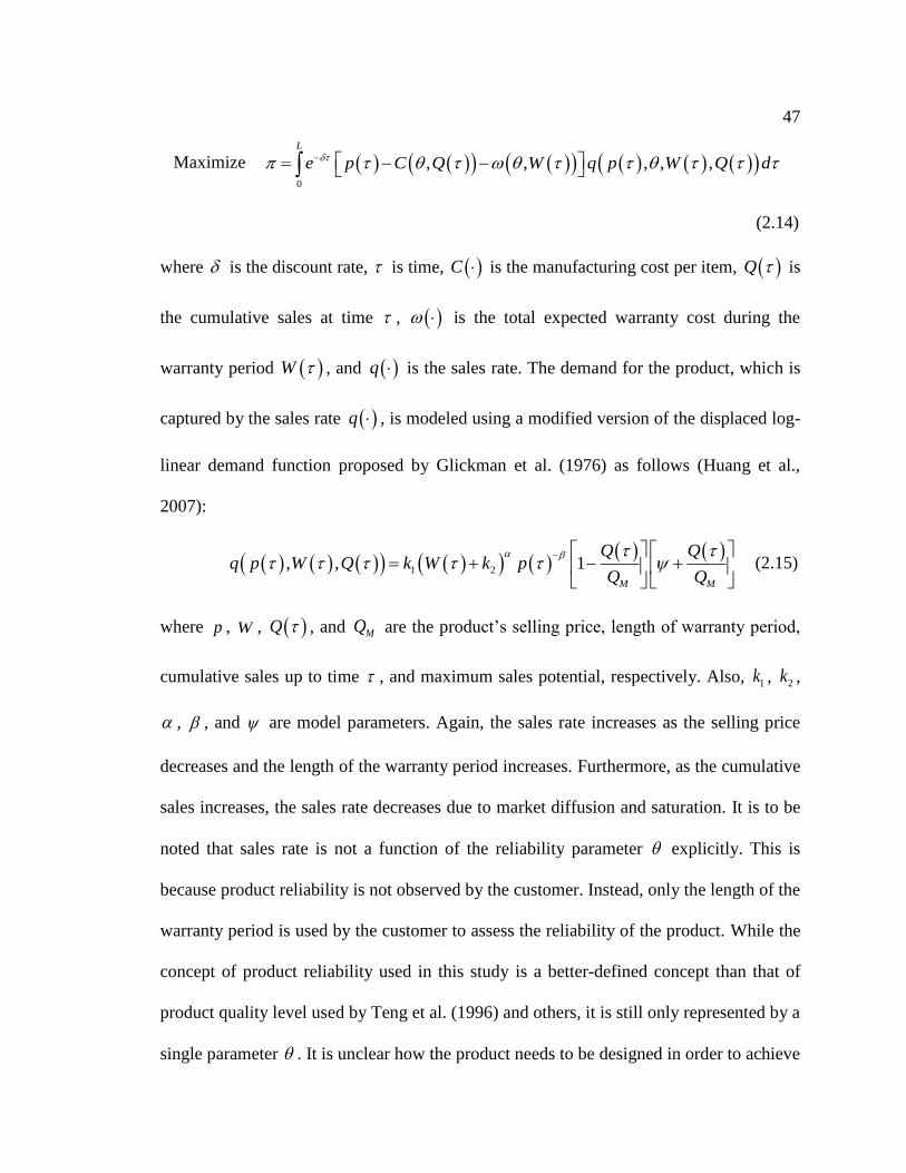
47

Maximize 0

, , , , ,

L

e p C Q W q p W Q d

(2.14)

where is the discount rate, is time, C is the manufacturing cost per item, Q is

the cumulative sales at time , is the total expected warranty cost during the

warranty period W , and q is the sales rate. The demand for the product, which is

captured by the sales rate q , is modeled using a modified version of the displaced log-

linear demand function proposed by Glickman et al. (1976) as follows (Huang et al.,

2007):

1 2, , 1M M

Q Qq p W Q k W k p

Q Q

(2.15)

where p , W , Q , and MQ are the product’s selling price, length of warranty period,

cumulative sales up to time , and maximum sales potential, respectively. Also, 1k , 2k ,

, , and are model parameters. Again, the sales rate increases as the selling price

decreases and the length of the warranty period increases. Furthermore, as the cumulative

sales increases, the sales rate decreases due to market diffusion and saturation. It is to be

noted that sales rate is not a function of the reliability parameter explicitly. This is

because product reliability is not observed by the customer. Instead, only the length of the

warranty period is used by the customer to assess the reliability of the product. While the

concept of product reliability used in this study is a better-defined concept than that of

product quality level used by Teng et al. (1996) and others, it is still only represented by a

single parameter . It is unclear how the product needs to be designed in order to achieve

48

a certain level of reliability. Thus, from a practical point of view, the way product

reliability is modeled in this study is in effect as vague as product quality level used in

the other studies.

Ladany et al. (2007) study the problem of finding the optimal length of the

warranty period while maximizing the total net profit for a given planning period. The

total net profit is given by (Ladany et al., 2007):

Q R c K (2.16)

where Q is the total quantity of the product sold during the planning period, R is the

expected revenue per item, c and K are the variable and fixed costs of manufacturing

and servicing the product, respectively. Here, Q is related to the selling price P and the

length of the warranty period w using the Cobb-Douglas-type demand function given by

(Ladany et al., 2007):

Q P w (2.17)

where , , and are model parameters. Furthermore, it is assumed that P is related to

w according to the linear relationship given by (Ladany et al., 2007):

P a bw (2.18)

where a and b are model parameters. In the proposed model, it is assumed that a longer

warranty period is an indication of higher quality, which results in higher demand for the

product for a given selling price. In addition, the length of the warranty period is related

to the lifetime distribution of the product. It is assumed that there are both lower and

upper specification limits for this lifetime distribution and that the manufacturer wants to

align the length of the warranty period with the lower specification limit of the product’s

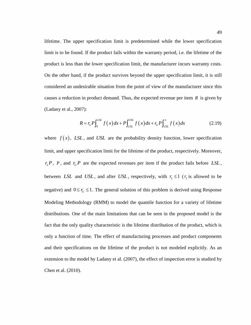
49

lifetime. The upper specification limit is predetermined while the lower specification

limit is to be found. If the product fails within the warranty period, i.e. the lifetime of the

product is less than the lower specification limit, the manufacturer incurs warranty costs.

On the other hand, if the product survives beyond the upper specification limit, it is still

considered an undesirable situation from the point of view of the manufacturer since this

causes a reduction in product demand. Thus, the expected revenue per item R is given by

(Ladany et al., 2007):

0

LSL USL

L ULSL USL

R r P f x dx P f x dx r P f x dx

(2.19)

where f x , LSL , and USL are the probability density function, lower specification

limit, and upper specification limit for the lifetime of the product, respectively. Moreover,

Lr P , P , and Ur P are the expected revenues per item if the product fails before LSL ,

between LSL and USL , and after USL , respectively, with 1Lr ( Lr is allowed to be

negative) and 0 1Ur . The general solution of this problem is derived using Response

Modeling Methodology (RMM) to model the quantile function for a variety of lifetime

distributions. One of the main limitations that can be seen in the proposed model is the

fact that the only quality characteristic is the lifetime distribution of the product, which is

only a function of time. The effect of manufacturing processes and product components

and their specifications on the lifetime of the product is not modeled explicitly. As an

extension to the model by Ladany et al. (2007), the effect of inspection error is studied by

Chen et al. (2010).

50

Sinha et al. (2011) study price and warranty competition in a duopoly market

structure. It is assumed that the two firms produce differentiated but substitutable

products. Each firm tries to maximize its total expected profit during a given planning

horizon while considering not only its own decisions about the product selling price and

the length of its warranty period, but also the competitor’s price and warranty decisions

as well. The total expected profit i for firm i during the planning horizon is given by

(Sinha et al., 2011):

i i i i i iD p c w

(2.20)

for 1,2i , where iD is the total demand during the planning horizon for product i , ip is

the selling price, is the manufacturing cost per item, i i ic w

is the warranty cost per

item since a Weibull lifetime distribution with scale parameters i and shape parameter

is assumed for each of the two products. iD is based on the demand function proposed

by Banker et al. (1998), which is given by (Banker et al., 1998):

i i i j i jD k p p x x (2.21)

for , 1,2i j and i j , where p is the selling price of the product, x is the quality level,

ik , , , , , and are nonnegative model parameters with 1 2 1k k , , and

. Sinha et al. (2011) modify equation (2.21) by replacing the quality levels ix with

the length of the warranty periods iw and ignoring the parameters ik , for 1,2i . With

this model, Nash-Bertrand equilibrium is derived for the cases of price competition alone,

warranty competition alone, and simultaneous price and warranty competitions.

51

Moreover, for each of these three competition cases, the multi-period dynamics of the

iterative interactions between the two competitors from the start of the competition until

reaching Nash-Bertrand equilibrium are studied. Furthermore, the case of coordination

between the two firms, as oppose to competition, is also considered. It is to be noted that,

while this study is quite detailed in terms of the important aspects of the duopoly market

structure, product design and its connection to product price and warranty are not

considered in any of the proposed models.

It can be seen from the literature review of this section that critical decisions

related to the selling price, quality level, warranty policy, production rate, etc., of the

product are made in the initial stages of product development based on customer and

market behaviors as well as manufacturing costs. Customer and market behaviors are

assessed in a fairly detailed manner in most of the studies. However, manufacturing costs

are modeled with very crude representations and simple equations, which compromise

the accuracy and optimality of the results obtained. Thus, it can be seen that the proposed

models of the studies reviewed in this section make many assumptions about the

production process, whereas the studies reviewed in section 2.1, i.e. integrated parameter

and tolerance designs without microeconomic and marketing considerations, make many

assumptions about the customer and market behaviors.

In this research, new integrated parameter and tolerance designs models are

proposed to address the main limitations of the previous studies. In Chapter 3, integrated

parameter and tolerance designs models are considered without discussing

microeconomic and marketing issues, such as pricing, market structure, customer utility

52

and demand functions, etc. Microeconomic and marketing issues are considered in the

integrated parameter and tolerance designs models of Chapter 4.

53

Chapter 3

Integrated Parameter and Tolerance Designs without Microeconomic and


In this chapter, new integrated parameter and tolerance designs models are

developed that resolve the main limitations of previous models discussed in the literature

review of section 2.1. Most importantly, the quadratic loss function that is used by all

studies to estimate quality losses is replaced with the warranty costs model. This is

because the warranty costs model is better defined conceptually when compared to the

quadratic loss function and is related to measurable quality attributes, such as product

reliability. With the use of the warranty and reliability models presented in sections 1.2.3

and 1.2.4, respectively, the deviation of the product quality characteristic from its ideal

value is related to warranty costs in an analogous manner as the way it is related to

external failure costs in the quadratic loss function.

3.1 Model Development

In this model, X is the main quality characteristic of a product and it is a function

of the quality characteristics of k components 1 2, ,..., kX X X . The functional form

1 2, ,..., kX e X X X , which defines the relationship between the main product

characteristic and the components characteristics, is assumed to be known. Starting with

the functional form 1 2, ,..., kX e X X X , Chandra (2001) shows that the mean and

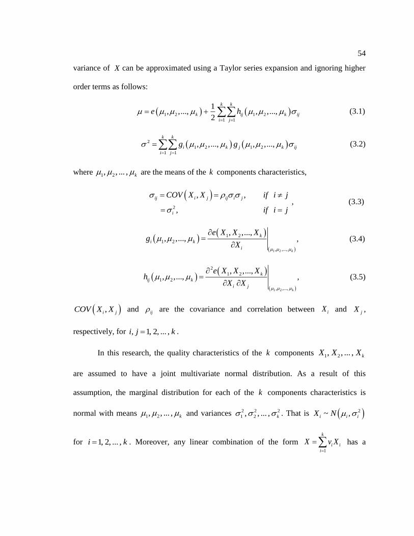
54

variance of X can be approximated using a Taylor series expansion and ignoring higher

order terms as follows:

1 2 1 2

1 1

1, ,..., , ,...,

2

k k

k ij k ij

i j

e h

(3.1)

2

1 2 1 2

1 1

, ,..., , ,...,k k

i k j k ij

i j

g g

(3.2)

where 1 2, , ... , k are the means of the k components characteristics,

2

, ,

,

ij i j ij i j

i

COV X X if i j

if i j

, (3.3)

1 2

1 2

1 2

, ,...,

, ,...,, ,...,

k

k

i k

i

e X X Xg

X

, (3.4)

1 2

2

1 2

1 2

, ,...,

, ,...,, ,...,

k

k

ij k

i j

e X X Xh

X X

, (3.5)

,i jCOV X X and ij are the covariance and correlation between iX and jX ,

respectively, for , 1, 2, ... ,i j k .

In this research, the quality characteristics of the k components 1 2, , ... , kX X X

are assumed to have a joint multivariate normal distribution. As a result of this

assumption, the marginal distribution for each of the k components characteristics is

normal with means 1 2, , ... , k and variances 2 2 2

1 2, , ... , k . That is 2~ ,i i iX N

for 1, 2, ... ,i k . Moreover, any linear combination of the form 1

k

i i

i

X v X

has a

55

univariate normal distribution with exact mean and variance, which are given by (Hogg,

2006):

1

k

i i

i

v

(3.6)

and

2

1 1

k k

i j ij

i j

v v

(3.7)

respectively, where i is the mean of the quality characteristic of component i for

1,2,...,i k and ij is the covariance term as defined in equation (3.3). It is worth

mentioning that it is quite common in practice for the k components characteristics

1 2, , ... , kX X X to be independent. That is why the majority of the studies in the literature

assume that 1 2, , ... , kX X X are independent in their models. Therefore, if the

independence of 1 2, , ... , kX X X is assumed, the mean and variance of the main product

characteristic X are reduced from equations (3.1) and (3.2) to:

2

1 2 1 2

1

1, ,..., , ,...,

2

k

k ii k i

i

e h

(3.8)

and

22 2

1 2

1

, ,...,k

i k i

i

g

(3.9)

where .ig and .iih are defined in equations (3.4) and (3.5), respectively.

Given the relationship between the main product characteristic and the

components characteristics, the idea of an integrated parameter and tolerance designs

model is to specify the means and the natural process tolerances (or equivalently the

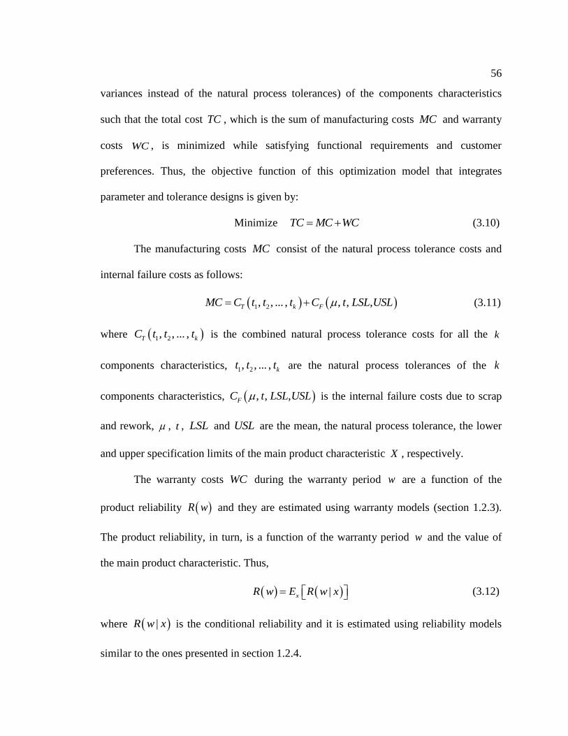
56

variances instead of the natural process tolerances) of the components characteristics

such that the total cost TC , which is the sum of manufacturing costs MC and warranty

costs WC , is minimized while satisfying functional requirements and customer

preferences. Thus, the objective function of this optimization model that integrates

parameter and tolerance designs is given by:

Minimize TC MC WC (3.10)

The manufacturing costs MC consist of the natural process tolerance costs and

internal failure costs as follows:

1 2, , ... , , , ,T k FMC C t t t C t LSL USL (3.11)

where 1 2, , ... ,T kC t t t is the combined natural process tolerance costs for all the k

components characteristics, 1 2, , ... , kt t t are the natural process tolerances of the k

components characteristics, , , ,FC t LSL USL is the internal failure costs due to scrap

and rework, , t , LSL and USL are the mean, the natural process tolerance, the lower

and upper specification limits of the main product characteristic X , respectively.

The warranty costs WC during the warranty period w are a function of the

product reliability R w and they are estimated using warranty models (section 1.2.3).

The product reliability, in turn, is a function of the warranty period w and the value of

the main product characteristic. Thus,

|xR w E R w x (3.12)

where |R w x is the conditional reliability and it is estimated using reliability models

similar to the ones presented in section 1.2.4.

57

It is to be noted that, since the marginal distribution for each of the k components

characteristics is normal and the range of all possible values of these characteristics is

infinite, it is conventional to define the natural process tolerances of the components

characteristics as:

6i it (3.13)

such that, it contains 99.73% of all possible values of the quality characteristic of

component i , for 1,2, ... ,i k . As a result of equation (3.13), the natural process

tolerance costs term in equation (3.11), i.e. 1 2, , ... ,T kC t t t , is in effect a relationship

between the costs and the variances of the k components characteristics. That is why the

natural process tolerances and the variances of the components characteristics can be

used interchangeably as decision variables in the optimization model. Moreover, the

natural process tolerance t of the main product characteristic X can be defined using

either the worst-case relationship or the probabilistic relationship, where the use of the

worst-case relationship results in tighter constraints on the tolerances of the components

characteristics and smaller failure rates (larger pkC ) than the use of the probabilistic

relationship. The worst-case relationship for t is defined as (Wu et al., 1998):

1 2

1

, ,...,k

i k i

i

t g t

(3.14)

where .ig is given by equation (3.4), i and it are the mean and the natural process

tolerance of the quality characteristic of component i , respectively, for 1,2, ... ,i k . The

probabilistic relationship for t , on the other hand, is derived starting with the relationship

58

for the variance of the main quality characteristic X of the product, i.e. equation (3.2),

which can be rewritten as:

22 2

1 2

1

1 2 1 2

, ,...,

2 , ,..., , ,...,

k

i k i

i

i k j k ij i j

i j

g

g g

(3.15)

for , 1, 2, ... ,i j k . Then, replacing the standard deviations 1 2, ..., k of the

components characteristics with the natural process tolerances 1 2, , ... , kt t t using equation

(3.13), equation (3.15) becomes:

222

1 2

1

1 2 1 2

, ,...,6

2 , ,..., , ,...,6 6

ki

i k

i

jii k j k ij

i j

tg

ttg g

Finally, is replaced with t G to give:

0.52 2

1 2

1

1 2 1 2

, ,...,

6 2 , ,..., , ,...,

k

i k i

i

i k j k ij i j

i j

g tG

tg g t t

(3.16)

where G is the coefficient that makes 100% or at least 99.73% of all possible values of

the main product characteristic X fall within the range G , i.e. t G . Examples for

G values include 6 for a normal distribution and 12 for a uniform distribution

(Chandra, 2001). If the distribution of X is unknown, empirical or simulated data can be

used, based on 1 2, ,..., kX e X X X and known 1 2, ,..., kX X X distributions, to estimate

the natural process tolerance t , which is the range of 100% or close to 100% of all

59

possible values of X . Then, G is calculated as the ratio of t and , where is

calculated from equation (3.2) or (3.15).

Besides the objective function (equation (3.10)), several constraints are added to

the optimization model in order to insure proper solutions. The means and standard

deviations of the components characteristics are constrained by minimum and maximum

values as follows:

min maxi i i (3.17)

min maxi i i (3.18)

for 1,2, ... ,i k . These constraints imply that even though the choices for the means and

standard deviations of the components characteristics are generally flexible, they are still

expected to be within certain ranges (Jeang et al., 2002b). The constraints in (3.17) are

imposed based on customer preferences and feasible process ranges while the constraints

in (3.18) are imposed based on available manufacturing processes and their capabilities.

Again, since the standard deviations and natural process tolerances of the components

characteristics are related as in equation (3.13), the constraints in (3.18) can be

equivalently presented as:

min maxi i it t t (3.19)

for, 1,2, ... ,i k . Furthermore, another constraint is added to insure that the resultant

natural process tolerance t of the main product characteristic X is not too wide from the

customer’s point of view. This constraint, which is typically referred to as the stack-up

constraint for t , is defined as:

60

min

2 min ,

pk

LSL USLt

C

(3.20)

where , minpkC , LSL , and USL are the mean, minimum allowable process capability

index, the lower and upper specification limits, respectively, for the main product

characteristic. Equation (3.20) is derived from the fact that, in order to guarantee the

achievement of an actual pkC that is at least equal to

minpkC , should be constrained as

follows:

min min

2 2pk pk

t tLSL C USL C (3.21)

Solving for t , the constraint in (3.21) becomes:

min

2

pk

LSLt

C

(3.22a)

and

min

2

pk

USLt

C

(3.22b)

which is equivalent to equation (3.20). Figure 3.1 illustrates the effect of imposing the

constraint of equation (3.20), where the distribution of the main product characteristic X

is normal and min 1pkC . Figures 3.1a and 3.1b show, respectively, the minimum and

maximum values of the mean of the main product characteristic that can be chosen while

the actual pkC is still at least equal to minpkC . Also, Figure 3.1c shows a general case

where the mean of the main product characteristic falls within the minimum and

maximum values such that the actual pkC is greater than minpkC .

61

Figure 3.1: Illustration of the stack-up constraint for t . a) The extreme case where is

as small as possible while maintaining , minpk actual pkC C , b) the other extreme case where

is as large as possible while maintaining , minpk actual pkC C , c) a general case where

, minpk actual pkC C . (Note: in the figures, the distribution of the main product characteristic

X is normal and min 1pkC ).

(c) t

USL min

max LSL

(b)

USL

t

min max

LSL

(a)

USL

t

min max LSL

62

If the ideal value 0x of the main product characteristic X is set at the midpoint

between the lower and upper specification limits, i.e. the allowable design tolerance

T USL LSL is balanced, then, the stack-up constraint for t of equation (3.20)

reduces to:

0

min

2

pk

T xt

C

(3.23)

where and minpkC are the mean and the minimum allowable process capability index,

respectively, for X . Again, equation (3.23) is derived in a similar manner as equation

(3.20) using the following constraint on :

0 min 0 min

2 2 2 2pk pk

T t T tx C x C (3.24)

Solving for t , the constraint in (3.24) becomes:

0

0

min

0

0

min

2,

2,

pk

pk

T xif x

Ct

T xif x

C

(3.25)

which is equivalent to equation (3.23).

3.2 Numerical Examples

In this section, several numerical examples are used to illustrate the methodology

of setting up and solving a verity of problems with different assumptions and challenges

based on the general optimization model for integrating parameter and tolerance designs

developed in section 3.1. Moreover, sensitivity analysis is conducted to validate the

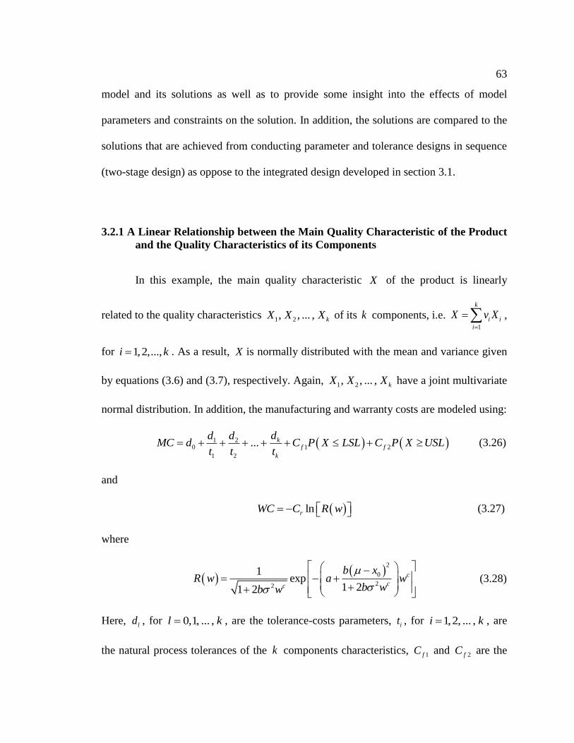
63

model and its solutions as well as to provide some insight into the effects of model

parameters and constraints on the solution. In addition, the solutions are compared to the

solutions that are achieved from conducting parameter and tolerance designs in sequence

(two-stage design) as oppose to the integrated design developed in section 3.1.

3.2.1 A Linear Relationship between the Main Quality Characteristic of the Product

and the Quality Characteristics of its Components

In this example, the main quality characteristic X of the product is linearly

related to the quality characteristics 1 2, , ... , kX X X of its k components, i.e. 1

k

i i

i

X v X

,

for 1,2,...,i k . As a result, X is normally distributed with the mean and variance given

by equations (3.6) and (3.7), respectively. Again, 1 2, , ... , kX X X have a joint multivariate

normal distribution. In addition, the manufacturing and warranty costs are modeled using:

1 20 1 2

1 2

... kf f

k

dd dMC d C P X LSL C P X USL

t t t (3.26)

and

lnrWC C R w (3.27)

where

2

0

22

1exp

1 21 2

c

cc

b xR w a w

b wb w

(3.28)

Here, ld , for 0,1, ... ,l k , are the tolerance-costs parameters, it , for 1,2, ... ,i k , are

the natural process tolerances of the k components characteristics, 1fC and 2fC are the

64

internal failure costs per item when X is less than LSL and X is greater than USL ,

respectively, LSL , USL , , 2 , and 0x are the lower specification limit, upper

specification limit, mean, variance, and ideal value for the main product characteristic,

respectively, rC is the warranty repair cost per item, , ,a b and c are the reliability

model’s parameters, and w is the length of the warranty period. Therefore, the

optimization model for integrating parameter and tolerance designs for this example has

an objective function (equation 3.10) that is calculated by summing equations (3.26) and

(3.27) subject to the constraints (3.17), (3.18) or (3.19), and (3.20).

3.2.1.1 Baseline Example

A simple numerical example for this model is presented for 1 2X X X . Thus,

X is normally distributed with mean 1 2 and variance 2 2 2

1 2 1 22 ., i.e.

2 2

1 2 1 2 1 2~ , 2X N . The optimization model seeks to determine the

optimal means and natural process tolerances (or variances instead of the natural process

tolerances according to equation (3.13)) of the two components characteristics that

minimize the total cost. This is a nonlinear optimization problem that can be solved using

programs, such as LINGO or Excel’s Solver. The data required for the model and the

values used in the baseline example are shown in Table 3.1.

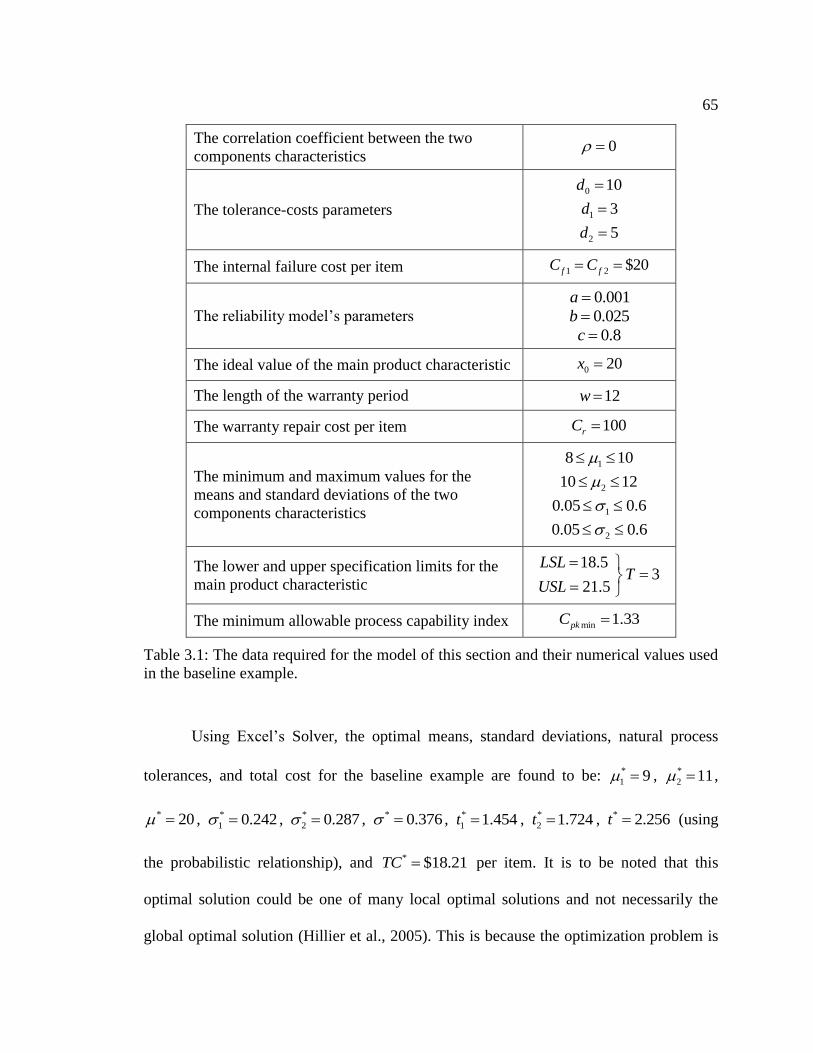
65

The correlation coefficient between the two

components characteristics 0

The tolerance-costs parameters

0 10d

1 3d

2 5d

The internal failure cost per item 1 2 $20f fC C

The reliability model’s parameters

0.001a

0.025b

0.8c

The ideal value of the main product characteristic 0 20x

The length of the warranty period 12w

The warranty repair cost per item 100rC

The minimum and maximum values for the

means and standard deviations of the two

components characteristics

18 10

210 12

10.05 0.6

20.05 0.6

The lower and upper specification limits for the

main product characteristic

18.53

21.5

LSLT

USL

The minimum allowable process capability index min 1.33pkC

Table 3.1: The data required for the model of this section and their numerical values used

in the baseline example.

Using Excel’s Solver, the optimal means, standard deviations, natural process

tolerances, and total cost for the baseline example are found to be: *

1 9 , *

2 11 ,

* 20 , *

1 0.242 , *

2 0.287 , * 0.376 , *

1 1.454t , *

2 1.724t , * 2.256t (using

the probabilistic relationship), and * $18.21TC per item. It is to be noted that this

optimal solution could be one of many local optimal solutions and not necessarily the

global optimal solution (Hillier et al., 2005). This is because the optimization problem is

66

nonlinear and the solution might depend on the initial values used to start the

optimization algorithm. This issue can be thoroughly investigated by studying the

convexity of the nonlinear problem’s objective function and constraints as well as

considering different initial values or even alternative optimization algorithms. However,

this matter is not pursued in this dissertation.

3.2.1.2 Sensitivity Analysis

Sensitivity analysis can be conducted by varying the assumptions and parameters

of the baseline example and studying the model behavior and solution in response to

these changes in model assumptions and parameters. Again, the purpose of conducting

sensitivity analysis is to validate the model and its solution as well as to gain some insight

into the effects of model assumptions, parameters, and constraints on the solution.

The effect of the correlation between 1X and 2X can be studied by considering

values for the correlation coefficient other than zero, where 1 1 . Table 3.2

shows the optimal means, standard deviations, the natural process tolerance of the main

product characteristic, process capability index, and total cost for several values of the

correlation coefficient (the optimal natural process tolerances 1t and 2t can be found

from the optimal standard deviations 1 and 2 using equation (3.13)).

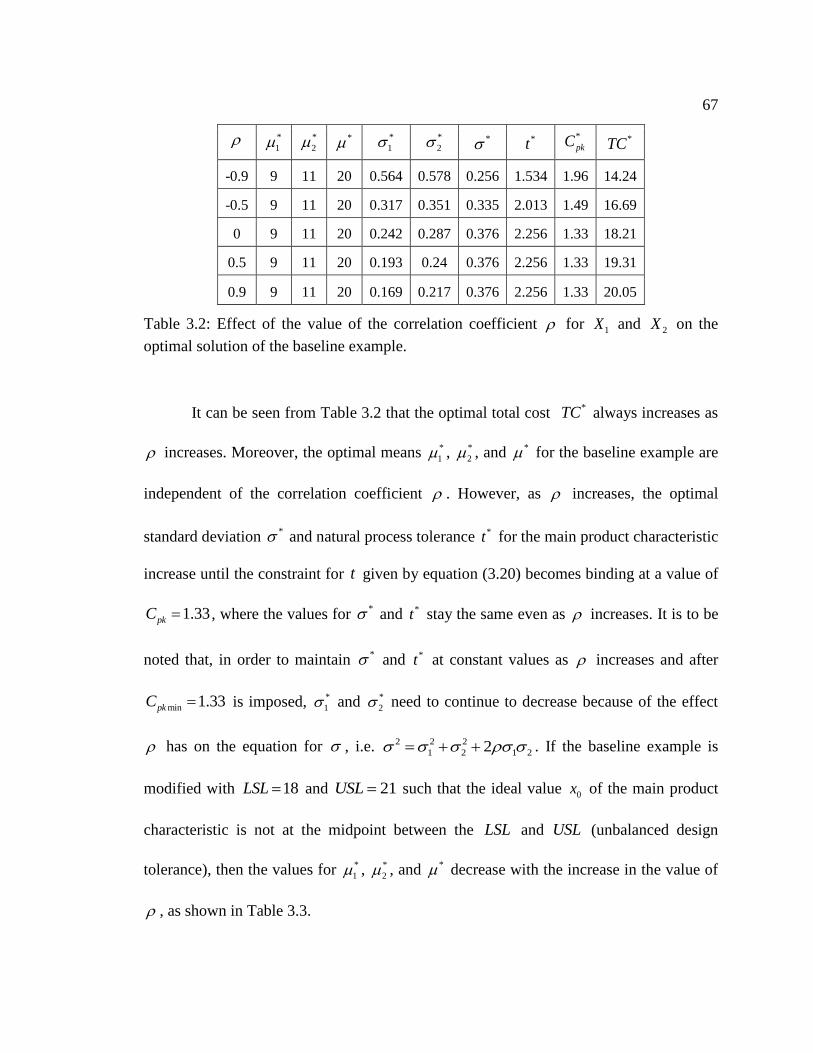
67

*

1 *

2 * *

1 *

2 * *t

*

pkC *TC

-0.9 9 11 20 0.564 0.578 0.256 1.534 1.96 14.24

-0.5 9 11 20 0.317 0.351 0.335 2.013 1.49 16.69

0 9 11 20 0.242 0.287 0.376 2.256 1.33 18.21

0.5 9 11 20 0.193 0.24 0.376 2.256 1.33 19.31

0.9 9 11 20 0.169 0.217 0.376 2.256 1.33 20.05

Table 3.2: Effect of the value of the correlation coefficient for 1X and

2X on the

optimal solution of the baseline example.

It can be seen from Table 3.2 that the optimal total cost *TC always increases as

increases. Moreover, the optimal means *

1 , *

2 , and * for the baseline example are

independent of the correlation coefficient . However, as increases, the optimal

standard deviation * and natural process tolerance *t for the main product characteristic

increase until the constraint for t given by equation (3.20) becomes binding at a value of

1.33pkC , where the values for * and *t stay the same even as increases. It is to be

noted that, in order to maintain * and *t at constant values as increases and after

min 1.33pkC is imposed, *

1 and *

2 need to continue to decrease because of the effect

has on the equation for , i.e. 2 2 2

1 2 1 22 . If the baseline example is

modified with 18LSL and 21USL such that the ideal value 0x of the main product

characteristic is not at the midpoint between the LSL and USL (unbalanced design

tolerance), then the values for *

1 , *

2 , and * decrease with the increase in the value of

, as shown in Table 3.3.

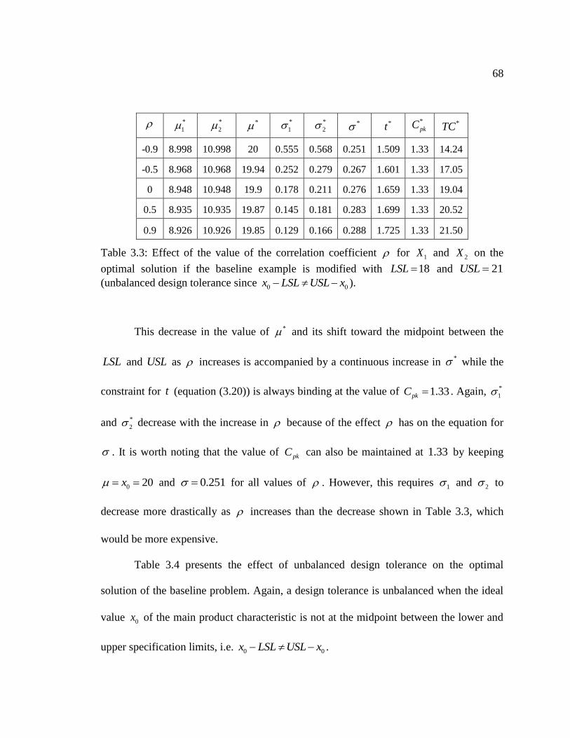
68

*

1 *

2 * *

1 *

2 * *t

*

pkC *TC

-0.9 8.998 10.998 20 0.555 0.568 0.251 1.509 1.33 14.24

-0.5 8.968 10.968 19.94 0.252 0.279 0.267 1.601 1.33 17.05

0 8.948 10.948 19.9 0.178 0.211 0.276 1.659 1.33 19.04

0.5 8.935 10.935 19.87 0.145 0.181 0.283 1.699 1.33 20.52

0.9 8.926 10.926 19.85 0.129 0.166 0.288 1.725 1.33 21.50

Table 3.3: Effect of the value of the correlation coefficient for 1X and 2X on the

optimal solution if the baseline example is modified with 18LSL and 21USL

(unbalanced design tolerance since 0 0x LSL USL x ).

This decrease in the value of * and its shift toward the midpoint between the

LSL and USL as increases is accompanied by a continuous increase in * while the

constraint for t (equation (3.20)) is always binding at the value of 1.33pkC . Again, *

1

and *

2 decrease with the increase in because of the effect has on the equation for

. It is worth noting that the value of pkC can also be maintained at 1.33 by keeping

0 20x and 0.251 for all values of . However, this requires 1 and 2 to

decrease more drastically as increases than the decrease shown in Table 3.3, which

would be more expensive.

Table 3.4 presents the effect of unbalanced design tolerance on the optimal

solution of the baseline problem. Again, a design tolerance is unbalanced when the ideal

value 0x of the main product characteristic is not at the midpoint between the lower and

upper specification limits, i.e. 0 0x LSL USL x .

69

LSL USL *

1 *

2 * *

1 *

2 * *t

*

pkC *TC

17.5 20.5 8.857 10.857 19.71 0.127 0.151 0.197 1.182 1.33 22.38

18 21 8.948 10.948 19.9 0.178 0.211 0.276 1.659 1.33 19.04

18.5 21.5 9 11 20 0.242 0.287 0.376 2.256 1.33 18.21

19 22 9.052 11.052 20.1 0.178 0.211 0.276 1.659 1.33 19.04

19.5 22.5 9.143 11.143 20.29 0.127 0.151 0.197 1.183 1.33 22.38

Table 3.4: Effect of unbalanced design tolerance ( 0 0x LSL USL x , with 0 20x ) on

the optimal solution of the baseline example.

As it can be seen in Table 3.4, when 0 20x shifts from the midpoint between

LSL and USL , * tends to be different from 0x and * decreases in order to satisfy the

constraint on t (equation (3.20)). This, in turn, results in an increase in *TC .

The constraint on t given by equation (3.20) is imposed, as mentioned

previously, to insure that the optimal solution, which minimizes the total costs, is not

obtained at an excessively wide value of t (low pkC ) that would be unsatisfactory to the

customer. Table 3.5 shows the effect of varying the value of minpkC in equation (3.20) on

the optimal solution of the baseline example.

70

minpkC *

1 *

2 * *

1 *

2 * *t

*

pkC *TC

0.67 9 11 20 0.243 0.288 0.377 2.261 1.327 18.21

1 9 11 20 0.243 0.288 0.377 2.261 1.327 18.21

1.33 9 11 20 0.242 0.287 0.376 2.256 1.33 18.21

1.67 9 11 20 0.193 0.229 0.299 1.796 1.67 18.57

2 9 11 20 0.161 0.191 0.25 1.5 2 19.32

Table 3.5: Effect of varying minpkC on the optimal solution of the baseline example.

It can be seen from Table 3.5 that minpkC values less than 1.327 result in the

constraint in equation (3.20) to be nonbinding. This means that the optimal solution

without imposing the constraint in equation (3.20) or when the constraint is nonbinding is

* $18.21TC , which is achieved at * 1.327pkC . For

minpkC values greater than 1.327, on

the other hand, the constraint in equation (3.20) is binding. This results in *

minpk pkC C

and *TC increasing with the increase in minpkC . It is worth emphasizing that the results in

Table 3.5 do not suggest that *TC increases monotonically with the increase in the value

of pkC used. In order to observe the effect of varying pkC on the optimal solution, the

constraint in equation (3.20) should be changed to equality. Figure 3.2 illustrates the

difference between the results obtained in Table 3.5 and the results that would be

obtained if the constraint in equation (3.20) is changed to equality.

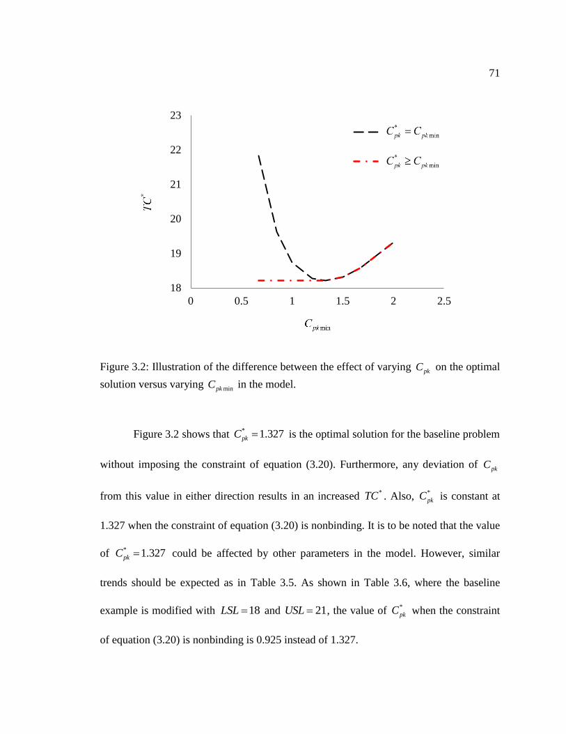
71

Figure 3.2: Illustration of the difference between the effect of varying pkC on the optimal

solution versus varying minpkC in the model.

Figure 3.2 shows that * 1.327pkC is the optimal solution for the baseline problem

without imposing the constraint of equation (3.20). Furthermore, any deviation of pkC

from this value in either direction results in an increased *TC . Also,

*

pkC is constant at

1.327 when the constraint of equation (3.20) is nonbinding. It is to be noted that the value

of * 1.327pkC could be affected by other parameters in the model. However, similar

trends should be expected as in Table 3.5. As shown in Table 3.6, where the baseline

example is modified with 18LSL and 21USL , the value of *

pkC when the constraint

of equation (3.20) is nonbinding is 0.925 instead of 1.327.

18

19

20

21

22

23

0 0.5 1 1.5 2 2.5

Cpk*=Cpkmin

Cpk*>=Cpkmin

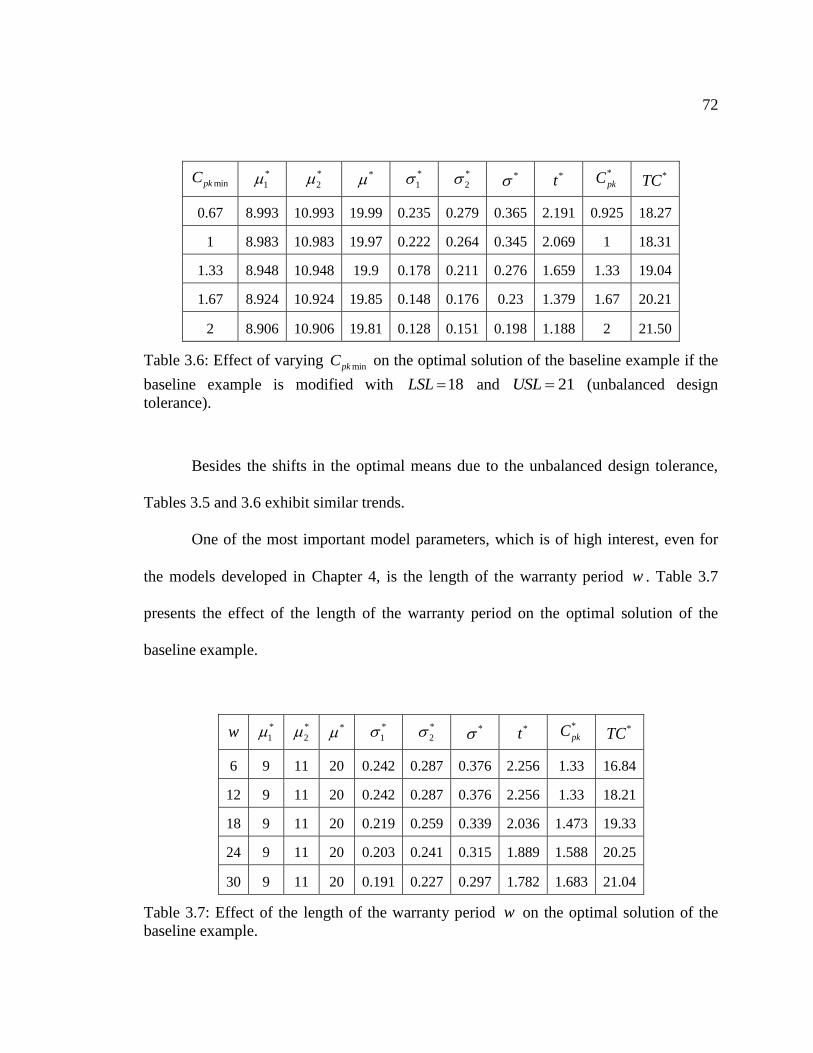
72

minpkC *

1 *

2 * *

1 *

2 * *t

*

pkC *TC

0.67 8.993 10.993 19.99 0.235 0.279 0.365 2.191 0.925 18.27

1 8.983 10.983 19.97 0.222 0.264 0.345 2.069 1 18.31

1.33 8.948 10.948 19.9 0.178 0.211 0.276 1.659 1.33 19.04

1.67 8.924 10.924 19.85 0.148 0.176 0.23 1.379 1.67 20.21

2 8.906 10.906 19.81 0.128 0.151 0.198 1.188 2 21.50

Table 3.6: Effect of varying minpkC on the optimal solution of the baseline example if the

baseline example is modified with 18LSL and 21USL (unbalanced design

tolerance).

Besides the shifts in the optimal means due to the unbalanced design tolerance,

Tables 3.5 and 3.6 exhibit similar trends.

One of the most important model parameters, which is of high interest, even for

the models developed in Chapter 4, is the length of the warranty period w . Table 3.7

presents the effect of the length of the warranty period on the optimal solution of the

baseline example.

w *

1 *

2 * *

1 *

2 * *t

*

pkC *TC

6 9 11 20 0.242 0.287 0.376 2.256 1.33 16.84

12 9 11 20 0.242 0.287 0.376 2.256 1.33 18.21

18 9 11 20 0.219 0.259 0.339 2.036 1.473 19.33

24 9 11 20 0.203 0.241 0.315 1.889 1.588 20.25

30 9 11 20 0.191 0.227 0.297 1.782 1.683 21.04

Table 3.7: Effect of the length of the warranty period w on the optimal solution of the

baseline example.

73

Table 3.7 shows that, not surprisingly, the optimal total cost *TC increases as the

length of the warranty w increases. Moreover, as w increases, *

pkC increases by

decreasing * and *t .

The results shown above are only a sample of the full sensitivity analysis that can

be conducted for every model assumption and parameter. There are obviously other

parameters and many interactions among these parameters and model constraints that

could be studied in a similar manner as the results shown above. However, since the idea

is to only show the methodology and some of the interesting results of conducting

sensitivity analysis, the full sensitivity analysis results are not presented.

3.2.1.3 Comparison between Sequential and Integrated Parameter and Tolerance

Designs

The sequential parameter and tolerance designs approach is a two-stage design

approach. In the first stage, parameter design is conducted using the Robust Parameter

Design (RPD) model of equation (1.8). Thus, for the simple example considered so far,

i.e. 1 2X X X , RPD determines the optimal 1 and 2 values for a given set of values

for 1 and 2 , such that, 0x and is minimized. Typically, for economical reasons,

1 and 2 are chosen to be large, i.e. low grade processes (Jeang, 2003). Then, in the

second stage, tolerance design is conducted by determining the optimal values for 1 and

2 (or equivalently 1t and 2t according to equation (3.13), hence the name tolerance

design) that minimize the total cost. Thus, this tolerance design uses the same objective

74

function and constraints as the integrated parameter and tolerance design developed in

this chapter except that 1 and 2 are predetermined from the RPD model.

Since 2 2

1 2 1 2 1 2~ , 2X N , the mean and variance 2 of X are

independent. Thus, the only situation where the integrated approach is superior to the

sequential approach is when the design tolerance for X is unbalanced such that 0x is not

at the midpoint between LSL and USL . Table 3.8 presents the effect of unbalanced

design tolerance on the optimal solution of the sequential parameter and tolerance design,

where 0 20x .

LSL USL *

1 *

2 * *

1 *

2 * *t

*

pkC *TC

17.5 20.5 9 11 20 0.081 0.096 0.125 0.752 1.33 25.90

18 21 9 11 20 0.162 0.192 0.251 1.504 1.33 19.31

18.5 21.5 9 11 20 0.242 0.287 0.376 2.256 1.33 18.21

19 22 9 11 20 0.162 0.192 0.251 1.504 1.33 19.31

19.5 22.5 9 11 20 0.081 0.096 0.125 0.752 1.33 25.90

Table 3.8: Effect of unbalanced design tolerance ( 0 0x LSL USL x , with 0 20x ) on

the optimal solution of the sequential parameter and tolerance designs.

Comparing Tables 3.4 and 3.8, it can be seen that, when the design tolerance is

unbalanced, the integrated approach results in better optimal solutions than the sequential

approach. Moreover, * is restricted to being always equal to 0x in the sequential

approach. This is in contrast to the integrated approach, where * can shift from 0x if

minimizing the total cost requires that.

75

3.2.2 A Nonlinear Relationship between the Main Quality Characteristic of the

Product and the Quality Characteristics of its Components

There are many forms of nonlinear relationships between the main quality

characteristic X of the product and the quality characteristics of its k components that

can be considered for analysis. However, since the purpose of this example is to present

the solution and analysis methodology for the nonlinear relationship case, a simple

nonlinear relationship is chosen for analysis. Thus, in this example, the relationship

between the main product characteristic X and the characteristics of only two product

components 1X and 2X is given by 1 2X X X . Due to this nonlinear relationship, the

distribution of X is treated as being unknown. Nonetheless, using equations (3.1) and

(3.2), the mean and variance of X can be approximated as 1 2 1 2 and

2 2 2 2 2

2 1 1 2 1 2 1 22 , respectively. Again, 1X and 2X have a joint

multivariate normal distribution with a correlation coefficient . In addition, the

manufacturing and warranty costs are modeled using:

1 20 1 2

1 2

f f

d dMC d C P X LSL C P X USL

t t (3.29)

and

ln |r xWC C E R w x (3.30)

where

2

0| exp cR w x a b x x w

(3.31)

76

Here, ld , for 0,1, 2l , are the tolerance-costs parameters,

it , for 1,2i , are the natural

process tolerances of the two components characteristics, 1fC and

2fC are the internal

failure costs per item when X is less than LSL and X is greater than USL ,

respectively, LSL , USL , x and 0x are the lower specification limit, upper specification

limit, observed value, and ideal value for the main product characteristic, respectively,

rC is the warranty repair cost per item, , ,a b and c are the reliability model’s

parameters, and w is the length of the warranty period. It is to be noted that the

unconditional reliability could not be represented in closed-form as in equation (3.28) due

to the nonlinear relationship between the main product characteristic and the two

components characteristics. That is why the conditional reliability is used in the model

instead (equation (3.31)). Therefore, the optimization model for integrating parameter

and tolerance designs has an objective function (equation 3.10) that is calculated by

summing equations (3.29) and (3.30) subject to the constraints (3.17), (3.18) or (3.19),

and (3.20).

3.2.2.1 Baseline Example

The data required for the model and the values used in the baseline example are

shown in Table 3.9.

77




0 10d

1 6d

2 10d



0.0001a

0.001b

0.8c


The length of the warranty period 12w





18 10

210 12

10.05 0.3

20.05 0.3



9020

110

LSLT

USL

The minimum allowable process capability index min 1.33pkC

Table 3.9: The data required for the model and their numerical values used in the baseline

example.

Again, since the unconditional reliability cannot be represented in closed-form

due to the nonlinear relationship 1 2X X X , which results in an unknown distribution for

X , the total cost, which is the objective function of the optimization model (equation

3.10), cannot be represented in closed-form either. As a result, conventional nonlinear

optimization algorithms cannot be used directly. Instead, the well-known Central

Composite Design (CCD) used in Response Surface Methodology (RSM) is employed to

78

find an approximate second-order objective function that relates the total cost to the

decision variables. This objective function is then minimized to achieve an approximate

optimal solution (Jeang, 2003). In this example, since the decision variables are the

means and standard deviations of the two components characteristics, i.e., 1 , 2 ,

1 ,

and 2 , a four factor CCD is used. The coded CCD for four factors as generated by

Minitab is given in Appendix A. Again, based on equation (3.13), the natural process

tolerances 1t and 2t could have been used instead of 1 and 2 as decision variables.

Table 3.10 shows a portion of the calculations for one replication used in the CCD

approach.

1 2 1 2 1x 2x x |R w x TC

8.5 10.5 0.113 0.113 8.492 10.770 91.46 0.587 87.03

9.5 10.5 0.113 0.113 9.396 10.657 100.14 0.999 33.79

8.5 11.5 0.113 0.113 8.623 11.430 98.56 0.984 35.29

9.5 11.5 0.113 0.113 9.425 11.632 109.63 0.508 101.52

8.5 10.5 0.238 0.113 8.417 10.598 89.20 0.426 114.25

9.5 10.5 0.238 0.113 9.293 10.554 98.08 0.973 31.78

8.5 11.5 0.238 0.113 8.286 11.642 96.47 0.912 38.19

9.5 11.5 0.238 0.113 9.724 11.552 112.33 0.329 140.07

8.5 10.5 0.113 0.238 8.587 10.518 90.33 0.505 94.31

Table 3.10: A portion of CCD calculations for the example of this section

79

Table 3.10 shows the uncoded values for 1 , 2 ,

1 , and 2 , which are obtained

from their allowable ranges provided in Table 3.9. Then, for each of the specific values of

1 , 2 , 1 , and 2 , random sample values,

1x and 2x , of the components characteristics

are generated, where 2~ ,i i iX N for 1, 2i , and the resultant main product

characteristic x is calculated using the relationship 1 2x x x . After that, |R w x is

found using equation (3.31) and the total cost is calculated by summing equations (3.29)

and (3.30). After replicating the CCD calculations several times, a second-order model is

fitted to the total cost TC as a function of 1 , 2 , 1 , and 2 . The second-order model

obtained for this example is:

1 2 1 2

2 2 2 2

1 2 1 2

1 2 1 1 1 2

2 1 2 2 1 2

28259 3149 2527 176 321.3

87.79 56.54 416 619.1

141.4 3.956 3.802

3.755 0.725 53.13

TC

(3.32)

with 2 68%R . Now, the optimization model for integrating parameter and tolerance

designs consists of an objective function that is given by equation (3.32) and is subject to

the constraints (3.17), (3.18) or (3.19), and (3.20). Using Excel’s Solver, the optimal

means, standard deviations, natural process tolerances, and total cost are found to be:

*

1 9.567 , *

2 10.45 , * 100 , *

1 0.162 , *

2 0.193 , * 2.506 , *

1 0.972t ,

*

2 1.159t , * 15.037t (using the probabilistic relationship), * $29.25TC per item.

When the correlation coefficient between the two components characteristics is

nonzero, the solution procedure is slightly modified to account for this correlation

between 1X and 2X . This is done by generating correlated random samples 1x and 2x in

80

the CCD calculations instead of the independent random samples used above (1x and

2x

columns in Table 3.10). Correlated random samples are obtained by first generating two

independent and identically distributed random samples from the standard normal

distribution, i.e. 1 2, ~ 0,1Z Z N , (Kroese et al., 2011). Then, 1X and 2X become

correlated random variables using the relationship:

11 1 1

22 2 22 2

0

1

X Z

X Z

(3.33)

where 1 , 2 , 1 , 2 , and are the means, standard deviations, and the correlation

coefficient of 1X and 2X , respectively. Also, the matrix

1

2

2 2

0

1C

is

obtained from the Cholesky decomposition as shown in Appendix B. After generating

correlated random samples, the same calculations and solution procedure are followed as

in the case for 0 shown above. It is worth noting that the same steps can be followed

to generate more than two correlated random variables using the appropriate C matrix,

which is obtained from the covariance matrix using the relationship TCC .

3.2.2.2 Sensitivity Analysis

Conducting sensitivity analysis for this example is not as straightforward as it is

shown for the example of section 3.2.1.2. This is because using the second-order fitted

relationship of equation (3.32) to conduct sensitivity analysis might not be appropriate

since this fitted relationship is only valid for the example parameters given in Table 3.9.

81

Therefore, any changes in the parameters of the original example could result in a

different fitted relationship between the total cost TC and the decision variables 1 , 2 ,

1 , and 2 . Nonetheless, sensitivity analysis can be conducted for a given parameter by

including this parameter as a decision variable in the fitted relationship for the total cost

TC . Another way to conduct sensitivity analysis, which is shown by Jeang (2003), is to

repeat the whole solution procedure for different values of the parameter of interest.

If the main product characteristic X is assumed to be normally distributed,

sensitivity analysis can be conducted in a similar manner as in section 3.2.1.2. This is

because equation (3.28) can be used for the unconditional reliability. As a result, the

model objective function, which is the total cost, is represented in closed-form by

summing the warranty and manufacturing costs of equations (3.28) and (3.29),

respectively. The normality assumption for X is quite appropriate for the parameter

values considered in this example as shown in Appendix C. It is to be noted that, even

though X is assumed to be normally distributed, its mean and variance are not

independent since 1 2 1 2 and 2 2 2 2 2

2 1 1 2 1 2 1 22 .

Table 3.11 presents the effect of the correlation coefficient on the optimal

solution of the baseline example.

82

*

1 *

2 * *

1 *

2 * *t

*

pkC *TC

-0.9 10 10.01 99.991 0.3 0.3 1.342 8.0527 2.481 20.26

-0.5 8.354 11.97 100 0.209 0.3 2.506 15.038 1.33 24.79

0 8.333 12 100 0.144 0.218 2.506 15.038 1.33 29.06

0.5 8.332 12 100 0.117 0.179 2.506 15.038 1.33 32.33

0.9 8.332 12 100 0.103 0.16 2.506 15.038 1.33 34.57

Table 3.11: Effect of the value of the correlation coefficient for 1X and

2X on the

optimal solution of the baseline example.

As it can be seen from Table 3.11, the optimal total cost *TC increases as

increases. Moreover, for 0.9 , even though 1 and 2 reach their maximum values

of 0.3 (given in Table 3.9), a low value for * is achieved with a

* 2.481pkC . Then, as

increases, *

1 and *

2 decrease to maintain * at 2.506 (

*

min 1.33pk pkC C ).

Table 3.12 shows the effect of unbalanced design tolerance, i.e.

0 0x LSL USL x , with 0 100x , on the optimal solution of the baseline example.

LSL USL *

1 *

2 * *

1 *

2 * *t

*

pkC *TC

85 105 8.178 12 98.138 0.099 0.152 1.72 10.32 1.33 35.68

87.5 107.5 8.25 12 98.995 0.123 0.187 2.132 12.789 1.33 31.05

90 110 8.333 12 100 0.144 0.218 2.506 15.038 1.33 29.06

92.5 112.5 8.41 12 100.92 0.121 0.182 2.11 12.661 1.33 31.22

95 115 8.483 12 101.79 0.098 0.146 1.702 10.214 1.33 36.09

Table 3.12: Effect of unbalanced design tolerance ( 0 0x LSL USL x , with 0 100x )

on the optimal solution of the baseline example.

83

It can be seen from Table 3.12 that, the more 0x shifts from the midpoint between

the LSL and USL , the higher are the optimal total cost *TC and the difference between

* and 0x . Moreover, in order to maintain *

pkC at 1.33 , * decreases as 0x shifts from

the midpoint between the LSL and USL .

The effect of the value of minpkC on the optimal solution of the baseline example

is shown in Table 3.13.

minpkC *

1 *

2 * *

1 *

2 * *t

*

pkC *TC

0.67 8.329 12 99.952 0.174 0.264 3.032 18.191 1.094 28.45

1 8.329 12 99.952 0.174 0.264 3.032 18.191 1.094 28.45

1.33 8.333 12 100 0.144 0.218 2.506 15.038 1.33 29.06

1.67 8.333 12 100 0.115 0.173 1.996 11.976 1.67 31.23

2 8.333 12 100 0.096 0.145 1.667 10 2 34.01

Table 3.13: Effect of varying minpkC on the optimal solution of the baseline example.

Table 3.13 shows that *

pkC is achieved at a value of 1.094 when minpkC is low. As

minpkC increases, the constraint on t (equation (3.20)) becomes binding, where

*

minpk pkC C . Thus, *TC is initially constant at 28.45 when * 1.094pkC . Then, *TC

increases with the increase in minpkC .

Lastly, the effect of the length of the warranty period w on the optimal solution

of the baseline example is presented in Table 3.14.

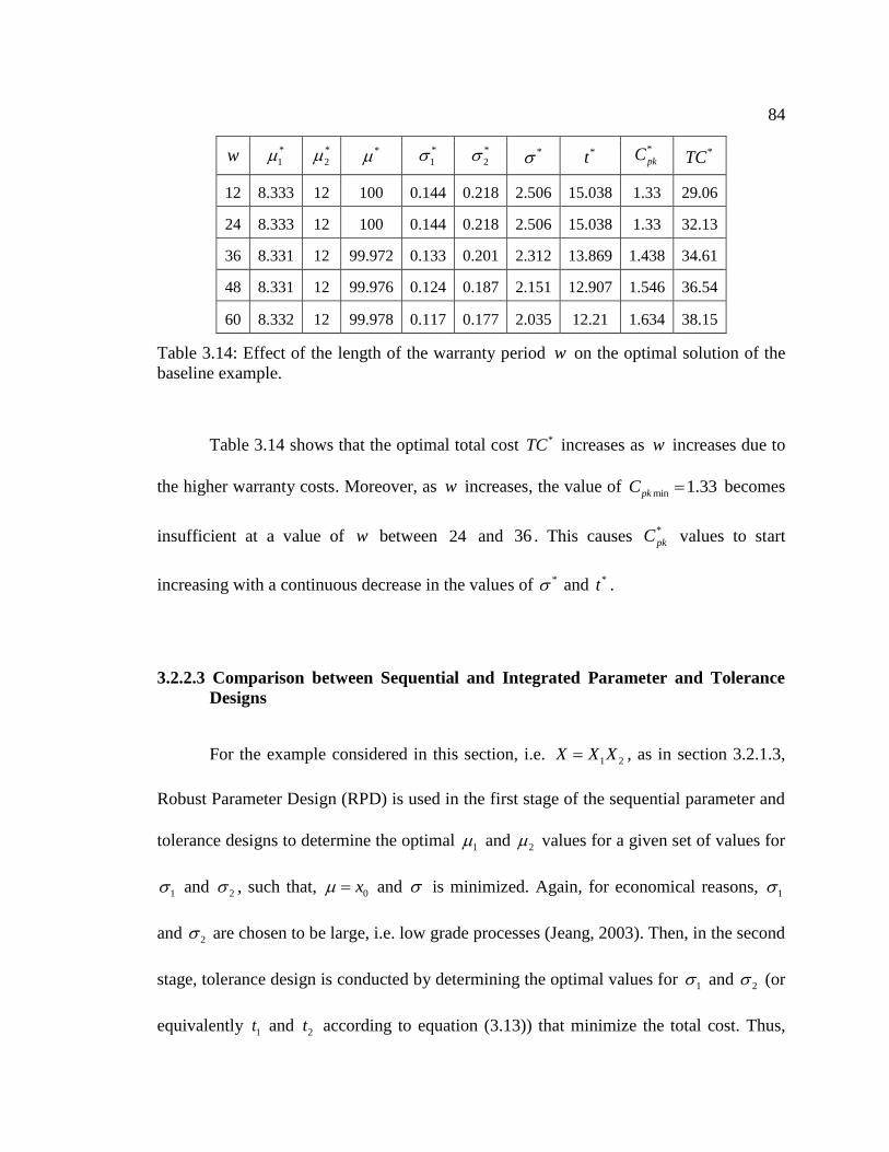
84

w *

1 *

2 * *

1 *

2 * *t

*

pkC *TC

12 8.333 12 100 0.144 0.218 2.506 15.038 1.33 29.06

24 8.333 12 100 0.144 0.218 2.506 15.038 1.33 32.13

36 8.331 12 99.972 0.133 0.201 2.312 13.869 1.438 34.61

48 8.331 12 99.976 0.124 0.187 2.151 12.907 1.546 36.54

60 8.332 12 99.978 0.117 0.177 2.035 12.21 1.634 38.15

Table 3.14: Effect of the length of the warranty period w on the optimal solution of the

baseline example.

Table 3.14 shows that the optimal total cost *TC increases as w increases due to

the higher warranty costs. Moreover, as w increases, the value of min 1.33pkC becomes

insufficient at a value of w between 24 and 36 . This causes *

pkC values to start

increasing with a continuous decrease in the values of * and *t .

3.2.2.3 Comparison between Sequential and Integrated Parameter and Tolerance

Designs

For the example considered in this section, i.e. 1 2X X X , as in section 3.2.1.3,

Robust Parameter Design (RPD) is used in the first stage of the sequential parameter and

tolerance designs to determine the optimal 1 and 2 values for a given set of values for

1 and 2 , such that, 0x and is minimized. Again, for economical reasons, 1

and 2 are chosen to be large, i.e. low grade processes (Jeang, 2003). Then, in the second

stage, tolerance design is conducted by determining the optimal values for 1 and 2 (or

equivalently 1t and 2t according to equation (3.13)) that minimize the total cost. Thus,

85

this tolerance design uses the same objective function and constraints as the integrated

parameter and tolerance design developed in this chapter except that 1 and 2 are

predetermined from the RPD model.

Once again, the normality assumption for 1 2X X X is assumed to be valid, as

verified in Appendix C. However, the mean 1 2 1 2 and variance

2 2 2 2 2

2 1 1 2 1 2 1 22 of X are not independent. Thus, unlike the example

presented in section 3.2.1.3, the integrated approach is superior to the sequential approach

in cases other than the case of an unbalanced design tolerance, i.e. 0 0x LSL USL x .

Table 3.15 presents the effect of the correlation coefficient on the optimal solution of

the sequential parameter and tolerance designs.

*

1 *

2 * *

1 *

2 * *t

*

pkC *TC

-0.9 10 10.01 100 0.3 0.3 1.342 8.0531 2.484 20.26

-0.5 9.996 10.01 100.01 0.236 0.262 2.503 15.017 1.33 25.04

0 10 10 100 0.162 0.192 2.506 15.038 1.33 29.35

0.5 9.995 10 99.965 0.128 0.16 2.498 14.985 1.33 32.67

0.9 9.992 10 99.933 0.112 0.144 2.49 14.938 1.33 34.96

Table 3.15: Effect of the correlation coefficient on the optimal solution of the

sequential parameter and tolerance designs.

A comparison between Tables 3.11 and 3.15 shows that, besides the case for

0.9 , where the maximum values of *

1 and *

2 of 0.3 are reached, the integrated

approach always results in better optimal solutions than the sequential approach. In

86

addition, Table 3.16 presents the effect of unbalanced design tolerance on the optimal

solution of the sequential parameter and tolerance designs, where 0 100x .

LSL USL *

1 *

2 * *

1 *

2 * *t

*

pkC *TC

85 105 10 10 100 0.081 0.096 1.253 7.5188 1.33 40.98

87.5 107.5 10 10 100 0.121 0.144 1.88 11.278 1.33 32.44

90 110 10 10 100 0.162 0.192 2.506 15.038 1.33 29.35

92.5 112.5 10 10 100 0.121 0.144 1.88 11.278 1.33 32.44

95 115 10 10 100 0.081 0.096 1.253 7.5188 1.33 40.98

Table 3.16: Effect of unbalanced design tolerance ( 0 0x LSL USL x , with 0 100x )

on the optimal solution of the sequential parameter and tolerance designs.

Comparing Tables 3.12 and 3.16, it can be seen that the integrated approach

always results in better optimal solutions than the sequential approach. Moreover, the

better results of the integrated approach are more profoundly exhibited as the shift of 0x

from the midpoint between LSL and USL becomes larger. Also, since *

1 and *

2 are

obtained from the first stage of the sequential approach, they are independent of the LSL

and USL .

3.2.3 Dealing with Discrete Tolerance-Costs Data Using Integer Programming

This example addresses the situation where the combined natural process

tolerance cost, i.e. tolerance-costs 1 2, , ... ,T kC t t t that appear in equation (3.11) for

manufacturing costs, is provided in the form of a table as opposed to a continuous

87

function. This is a more realistic situation in real life problems since typically there are

only a finite number of available manufacturing processes. Consequently, using the

continuous tolerance-costs function in the optimization model could result in

manufacturing processes that do not exist. Table 3.17 presents an example of a tolerance-

costs data set for the quality characteristics of two components that constitute a given

product.

Component i Process l 6

ilil

t Unit Cost ilD $

1

1 0.1 35

2 0.2 20

3 0.3 15

2

1 0.1 55

2 0.2 30

3 0.25 25

Table 3.17: Example of a tolerance-costs data list for the quality characteristics of two

components of a product.

Table 3.17 shows 2k components each of which having 3im available

processes for their manufacturing. Also, the standard deviation of the quality

characteristic of component i that manufacturing process l is capable of achieving and

the corresponding cost per unit produced ilD are shown in Table 3.17 as well.

The optimization model for integrating parameter and tolerance designs for this

example still consists of an objective function (equation 3.10) that is calculated by

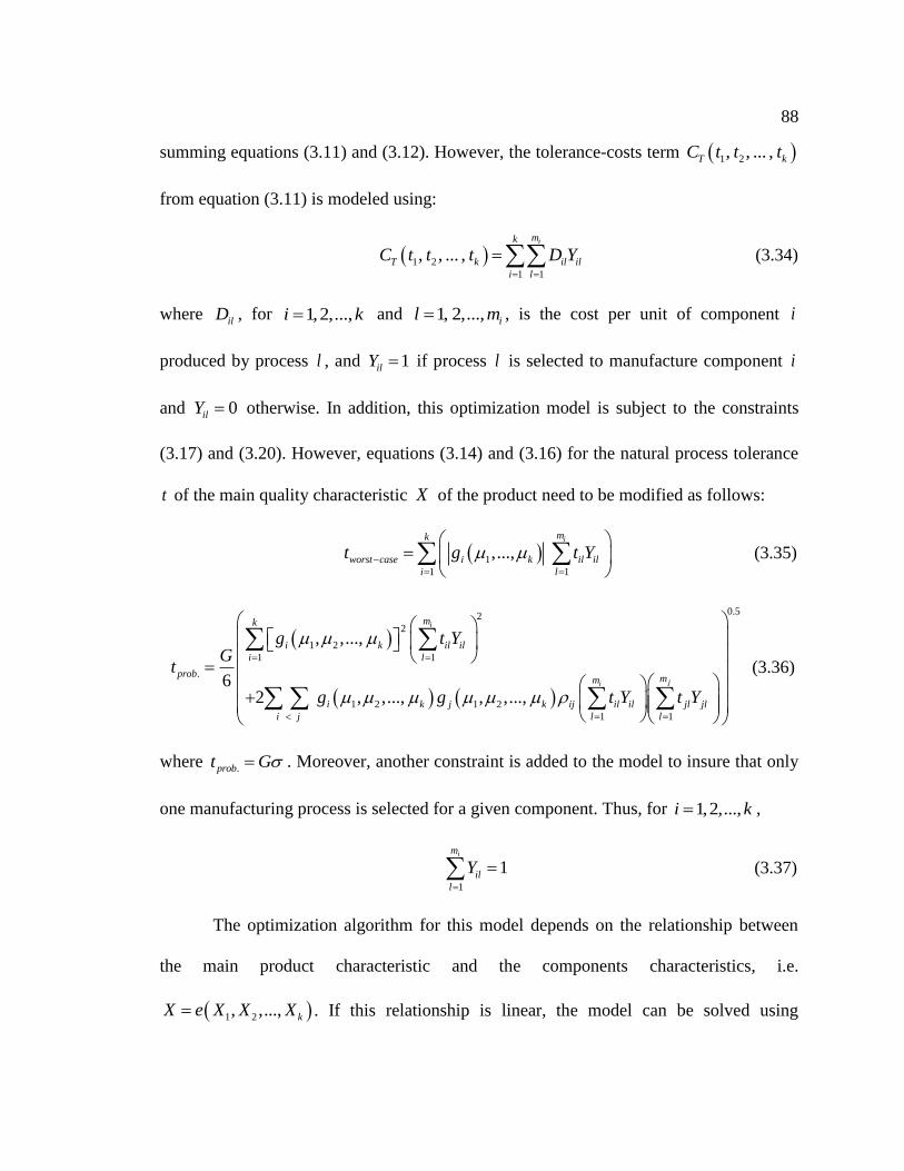
88

summing equations (3.11) and (3.12). However, the tolerance-costs term 1 2, , ... ,T kC t t t

from equation (3.11) is modeled using:

1 2

1 1

, , ... ,imk

T k il il

i l

C t t t D Y

(3.34)

where ilD , for 1,2,...,i k and 1, 2,..., il m , is the cost per unit of component i

produced by process l , and 1ilY if process l is selected to manufacture component i

and 0ilY otherwise. In addition, this optimization model is subject to the constraints

(3.17) and (3.20). However, equations (3.14) and (3.16) for the natural process tolerance

t of the main quality characteristic X of the product need to be modified as follows:

1

1 1

,...,imk

worst case i k il il

i l

t g t Y

(3.35)

0.52

2

1 2

1 1

.

1 2 1 2

1 1

, ,...,

62 , ,..., , ,...,

i

ji

mk

i k il il

i l

probmm

i k j k ij il il jl jl

i j l l

g t YG

t

g g t Y t Y

(3.36)

where .probt G . Moreover, another constraint is added to the model to insure that only

one manufacturing process is selected for a given component. Thus, for 1,2,...,i k ,

1

1im

il

l

Y

(3.37)

The optimization algorithm for this model depends on the relationship between

the main product characteristic and the components characteristics, i.e.

1 2, ,..., kX e X X X . If this relationship is linear, the model can be solved using

89

programs, such as LINGO or Excel’s Solver as in section 3.2.1. On the other hand, if the

relationship 1 2, ,..., kX e X X X is nonlinear and the distribution for X is unknown,

the model can be solved using the same solution methodology as in section 3.2.2.

However, the standard deviations 1 2, ,..., k of the k components characteristics are

treated as continuous variables when fitting the second-order relationship (using the CCD

approach) between the total cost TC and the means 1 2, ,..., k and standard deviations

1 2, ,..., k of the k components characteristics. Then, 1 2, ,..., k are replaced with

1

im

il il

l

Y

or 1 6

im

il il

l

t Y

, for 1,2,...,i k and 1, 2,..., il m , and the model is optimized.

3.3 Discussion

The integrated parameter and tolerance designs models proposed in this chapter

are flexible enough to handle a wide range of real-life problems. This is evident from the

different variety of models, numerical examples, and solution methodologies presented in

this chapter. However, it is important to realize that the proposed models are by no means

exhaustive or rigidly applicable to every real-life problem. The models used in the

numerical examples represent only a sample of the different reliability, warranty, and

manufacturing costs models that can be used. Furthermore, there are other issues that can

be considered within the same framework of the proposed models. These issues include

setup costs, monitoring and control costs, maintenance costs, measurement error

considerations, updating model parameters (adaptive models), etc. Again, the focus of

this chapter has been mainly to show the merit of using integrated models for parameter

90

and tolerance designs and the benefit of using well-defined and empirically measurable

concepts in the models. Consequently, it is left to the designers and engineers to select

the appropriate model components that best fit their application.

It is to be noted that one area of concern about the proposed models of this

chapter is the fact that finding a solution for the models could be time consuming or even

impossible when the size of the problem is large. This concern is especially relevant

when there is a nonlinear relationship between the main quality characteristic of the

product and the quality characteristics of the components. Obviously, this issue can be

addressed, at least partially, with advances in computer-related technologies, better

optimization algorithms, etc. However, even if the size of the problem is a concern, it is

worth emphasizing that the usefulness of the proposed models is not limited to solving

the full model for a new product. Instead, the proposed models can be used to study the

economic viability (return-on-investment decisions) of certain adjustments in the design,

manufacturing processes, warranty policies, etc., of existing products as well. That is, the

proposed models that integrate all major parameters, decision variables, and constraints

can be used to study the effects of changing a small number of model parameters,

constraints, or variables of interest.

Another issue that is important to mention is the viability of replacing the

quadratic loss function with warranty costs. As stated previously, one of the main

contributions of the models developed in this chapter for integrating parameter and

tolerance designs is replacing the quadratic loss function with warranty costs. Again, the

quadratic loss function suffers from its simplistic formulation making it difficult to

estimate external failure costs accurately. Warranty costs, on the other hand, are based on

91

solid empirical and financial grounds where they are related to the quality characteristics

of the product through the use of warranty and reliability models. However, the quadratic

loss function by definition encompasses all external failure costs, part of which is the

warranty costs. Thus, there exists the risk of underestimating the external failure costs

when the quadratic loss function is replaced with warranty costs. This underestimation is

compensated for by including the constraint on t (equation (3.20)) and the specification

of minpkC in the proposed models. The minimum allowable process capability index

minpkC introduces the voice of the customer in the proposed models through specifying

the minimum level of conformance quality required by the customer. Then again,

determining the appropriate value for minpkC that is satisfactory to the customer and both

technologically and economically viable for the manufacturer could be a challenge.

Addressing the issue of underestimating external failure costs when the quadratic loss

function is replaced with warranty costs is the topic of Chapter 4.

92

Chapter 4

Integrated Parameter and Tolerance Designs with Microeconomic and Marketing

Considerations

One of the key features of the integrated parameter and tolerance designs models

of Chapter 3 is the replacement of the quadratic loss function with warranty costs. Due to

the simple form of the quadratic loss function and the vague definition of its loss to

society parameter, estimating external failure costs using the quadratic loss function can

be quite a challenge in real-life problems. Warranty models are both conceptually and

mathematically sound and can be developed using reliability models and empirical data.

If the warranty costs are the only major external failure costs to the manufacturer and any

other losses, such as loss of customer’s trust, loss of market-share, lawsuits, etc., are so

minimal or inconsequential that they can be neglected, then replacing the quadratic loss

function with the warranty costs is justified. However, if external failure costs other than

warranty costs cannot be neglected, then replacing the quadratic loss function with the

warranty costs alone results in underestimated external failure costs, which would affect

the appropriateness of the proposed models and their solutions. Therefore, this chapter

introduces integrated parameter and tolerance designs models that address external failure

costs other than the ones covered under warranty by modeling their effects on customer

utility and product demand instead of treating them as actual costs that require listing and

estimation in monetary values. This is achieved by introducing microeconomic and

marketing concepts, such as pricing models, market structure types, consumer and

93

competitor behaviors, etc., into the integrated models and relating the customer utility

function or the demand function to the purchase price and product quality.

It is typical to assume that the price a customer is willing to pay for a given

product increases as the quality of the product increases. The key idea is that the increase

in purchase price for a higher quality product relative to another lower quality one

reflects, among other decision making criteria, the customer’s assessment of external

failure costs other than the warranty costs covered by the manufacturer. That is why, a

four-year-old used car with a mileage of 60,000 miles, for instance, can be as attractive as

a new car of the same model and options if its purchase price is significantly lower than

that of the new car, even for a customer who can afford the new car. This is because the

difference in price compensates for the obvious difference in quality (especially the

perceived reliability) making the two cars comparable in terms of customer utility. Again,

this approach is quite different from the approach of the quadratic loss function that tries

to list all possible losses to the manufacturer, customer, and the society as a whole and

estimate their monetary costs as a function of conformance quality.

4.1 Model Development

In the development of new products, information about the customer and the

market has to be known beforehand since this information greatly influences the analysis

approach and solution methodology. This is because different rules, dynamics, and

challenges are exhibited depending on the type of the market structure, i.e. monopoly,

oligopoly, perfect competition, etc., and depending on considering a static or a dynamic

94

market analysis approach. For instance, for the case of a monopoly in a static market,

Karmarkar et al. (1997) suggest maximizing the profit while satisfying a certain level of

customer utility. On the other hand, for the case of a perfect competition also in a static

market, it is suggested to maximize customer’s utility while maintaining a nonnegative

profit. These two models are given by (Karmarkar et al., 1997):

Maximize P TC (4.1a)

Subject to: 0U u (4.1b)

and

Maximize U (4.2a)

Subject to: 0P TC (4.2b)

where P is the selling price of an item, TC is the total cost of producing an item, U is

the expected customer utility, 0u is the minimum acceptable customer utility. However,

in the case of a dynamic market, models (4.1) and (4.2) are not sufficient. This is because

the effects of market dynamics, i.e. product expansion and saturation in the market,

learning effects, imitators and innovators influences, price variations, etc., over time

cannot be captured by these models. Instead, the model by Teng et al. (1996), for

instance, can be used. This model is given by equation (2.10) and it is shown here again

for convenience (Teng et al., 1996):

Maximize 0

, , ,

L

e p C q Q Q p q Q d (4.3)

where is the total present value of profit over the planning time horizon L , is the

discount rate, p is the selling price at time , C is the manufacturing cost per

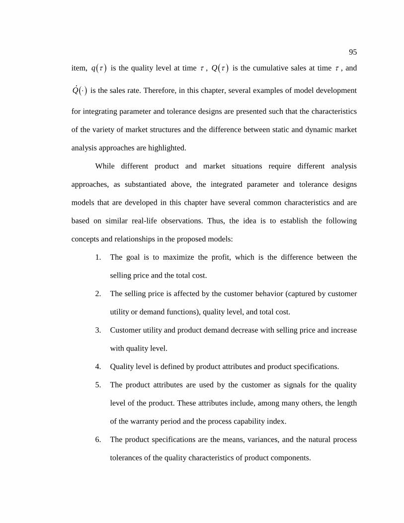
95

item, q is the quality level at time , Q is the cumulative sales at time , and

Q is the sales rate. Therefore, in this chapter, several examples of model development

for integrating parameter and tolerance designs are presented such that the characteristics

of the variety of market structures and the difference between static and dynamic market

analysis approaches are highlighted.

While different product and market situations require different analysis

approaches, as substantiated above, the integrated parameter and tolerance designs

models that are developed in this chapter have several common characteristics and are

based on similar real-life observations. Thus, the idea is to establish the following

concepts and relationships in the proposed models:

1. The goal is to maximize the profit, which is the difference between the

selling price and the total cost.

2. The selling price is affected by the customer behavior (captured by customer

utility or demand functions), quality level, and total cost.

3. Customer utility and product demand decrease with selling price and increase

with quality level.

4. Quality level is defined by product attributes and product specifications.

5. The product attributes are used by the customer as signals for the quality

level of the product. These attributes include, among many others, the length

of the warranty period and the process capability index.

6. The product specifications are the means, variances, and the natural process

tolerances of the quality characteristics of product components.

96

7. Product attributes and specifications along with the selling price are the

decision variables of the integrated models.

8. Total cost is the sum of manufacturing and warranty costs. These costs

depend on the quality level of the product, which in turn depends on product

attributes and specifications.

For simplicity, in all of the examples of this chapter, the relationship between the

main quality characteristic X of the product that is being designed and the quality

characteristics of the product’s only two components 1X and 2X is given by

1 2X X X . Thus, similar to the baseline example of section 3.2.1.1,

2 2

1 2 1 2 1 2~ , 2X N , where 1X and 2X have a multivariate normal

distribution with a correlation coefficient . In addition, the manufacturing and warranty

costs are modeled using:

1 20 1 2

1 2

f f

d dMC d C P X LSL C P X USL

t t (4.4)

and

lnrWC C R w (4.5)

where

2

0

22

1exp

1 21 2

c

cc

b xR w a w

b wb w

(4.6)

Here, ld , for 0,1, 2l , are the tolerance-costs parameters, it , for 1,2i , are the natural

process tolerances of the two components characteristics, 1fC and 2fC are the internal

97

failure costs per item when X is less than LSL and X is greater than USL ,

respectively, LSL , USL , , 2 , and 0x are the lower specification limit, upper

specification limit, mean, variance, and ideal value for the main product characteristic,

respectively, rC is the warranty repair cost per item, , ,a b and c are the reliability

model’s parameters, and w is the length of the warranty period. Moreover, the values of

the model parameters and constraints, which are common among all of the examples

presented in this chapter, are given in Table 4.1.




0 10d

1 3d

2 5d



0.001a

0.025b

0.8c






18 10

210 12

10.05 0.6

20.05 0.6



18.53

21.5

LSLT

USL

Table 4.1: The values of the model parameters and constraints that are common among

all the examples of the integrated models presented in this chapter.

98

It is worth mentioning that the constraint on the natural process tolerance t of the

main product characteristic X , which is given by equation (3.20) and used in the models

of Chapter 3, is unnecessary for the models of this chapter since the voice of the customer

is captured by the customer utility or demand functions.

4.1.1 Example 1: Using a Demand Function to Capture Total Sales during a Given

Planning Horizon

This example follows a similar modeling approach as the study by Ladany et al.

(2007), which is one of the simplest cases where pricing models and demand functions

are used for warranty decisions. The objective function of the integrated parameter and

tolerance designs model is given by:

Maximize P MC WC Q (4.7)

where is the total profit during a given planning horizon, P is the selling price of an

item, MC and WC are the manufacturing and warranty costs per item, which are given

by equations (4.4) and (4.5), respectively, and Q is the total quantity demanded (total

sales) during the planning horizon, which is given by (Ladany et al., 2007):

Q P w (4.8)

where is a proportionality constant, P is again the selling price, w is the length of the

warranty period, which is used as the only signal for the product quality level observed

by the customer, ( 1 ) and ( 0 1 ) are the selling price elasticity and the length

of the warranty period elasticity, respectively (Huang et al., 2007). It can be seen from

equation (4.8) that Q increases as P decreases and w increases. Moreover, as and

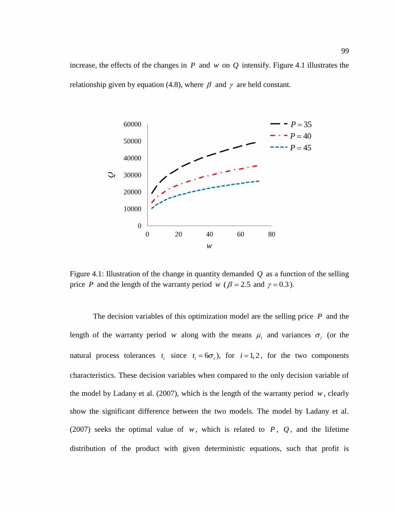
99

increase, the effects of the changes in P and w on Q intensify. Figure 4.1 illustrates the

relationship given by equation (4.8), where and are held constant.

Figure 4.1: Illustration of the change in quantity demanded Q as a function of the selling

price P and the length of the warranty period w ( 2.5 and 0.3 ).

The decision variables of this optimization model are the selling price P and the

length of the warranty period w along with the means i and variances i (or the

natural process tolerances it since 6i it ), for 1,2i , for the two components

characteristics. These decision variables when compared to the only decision variable of

the model by Ladany et al. (2007), which is the length of the warranty period w , clearly

show the significant difference between the two models. The model by Ladany et al.

(2007) seeks the optimal value of w , which is related to P , Q , and the lifetime

distribution of the product with given deterministic equations, such that profit is

0

10000

20000

30000

40000

50000

60000

0 20 40 60 80

Series1

Series2

Series3

w

35P

40P

45P

100

maximized. Parameter and tolerance designs, which are the focus of the models in this

dissertation, are not considered in their model.

The values of the model parameters and constraints used in this example, besides

the ones that are already shown in Table 4.1, are given in Table 4.2.

The total demand function parameters

100,000,000

2.5

0.3

The minimum and maximum price values 0 60P

The minimum and maximum values for the length

of the warranty period 3 72w

The minimum and maximum total product

quantity demanded during the planning horizon 0 200,000Q

Table 4.2: The values of the model parameters and constraints that are specific to the

example of this section.

Using Excel’s Solver, the optimal selling price, length of the warranty period,

means, standard deviations, natural process tolerances, process capability index, quantity

demanded, and total profit during the planning horizon for this example are found to be:

* 38.25P , * 47.56w , *

1 9 , *

2 11 , * 20 , *

1 0.170 , *

2 0.201 , * 0.263 ,

*

1 1.019t , *

2 1.208t , * 1.581t (using the probabilistic relationship), * 1.898pkC ,

* 35196Q , and * $538,551.89 .

In this example, two of the key parameters that appear in the integrated model are

the selling price elasticity and the length of the warranty period elasticity . These

two parameters represent the sensitivity of the demand for the product (the customer’s

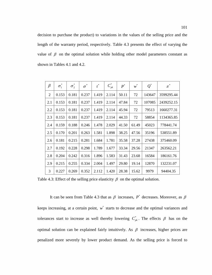
101

decision to purchase the product) to variations in the values of the selling price and the

length of the warranty period, respectively. Table 4.3 presents the effect of varying the

value of on the optimal solution while holding other model parameters constant as

shown in Tables 4.1 and 4.2.

*

1 *

2 * *t

*

pkC *P *w

*Q *

2 0.153 0.181 0.237 1.419 2.114 50.11 72 143647 3599295.44

2.1 0.153 0.181 0.237 1.419 2.114 47.84 72 107085 2439252.15

2.2 0.153 0.181 0.237 1.419 2.114 45.94 72 79513 1660277.31

2.3 0.153 0.181 0.237 1.419 2.114 44.33 72 58854 1134365.85

2.4 0.159 0.188 0.246 1.478 2.029 41.50 61.49 45023 778441.74

2.5 0.170 0.201 0.263 1.581 1.898 38.25 47.56 35196 538551.89

2.6 0.181 0.215 0.281 1.684 1.781 35.58 37.28 27438 375460.09

2.7 0.192 0.228 0.298 1.789 1.677 33.34 29.56 21347 263562.21

2.8 0.204 0.242 0.316 1.896 1.583 31.43 23.68 16584 186161.76

2.9 0.215 0.255 0.334 2.004 1.497 29.80 19.14 12870 132231.07

3 0.227 0.269 0.352 2.112 1.420 28.38 15.62 9979 94404.35

Table 4.3: Effect of the selling price elasticity on the optimal solution.

It can be seen from Table 4.3 that as increases, *P decreases. Moreover, as

keeps increasing, at a certain point, *w starts to decrease and the optimal variances and

tolerances start to increase as well thereby lowering *

pkC . The effects has on the

optimal solution can be explained fairly intuitively. As increases, higher prices are

penalized more severely by lower product demand. As the selling price is forced to

102

decrease, offering long warranty periods becomes more difficult and financially

unjustifiable. As a result of the shorter warranty periods in addition to the lower selling

prices, it becomes unnecessary to maintain high levels of pkC values. Therefore,

pkC is

lowered by increasing the variances.

The effect of varying the value of on the optimal solution while holding other

model parameters constant is shown in Table 4.4.

*

1 *

2 * *t

*

pkC *P *w

*Q *

0.15 0.315 0.373 0.488 2.930 1.024 26.46 3.842 33975 359611.84

0.175 0.286 0.340 0.444 2.666 1.125 27.82 6.09 33618 374048.17

0.2 0.255 0.303 0.396 2.378 1.262 29.53 9.838 33323 393677.17

0.225 0.227 0.269 0.352 2.112 1.420 31.53 15.62 33241 419284.39

0.25 0.204 0.242 0.316 1.896 1.583 33.68 23.68 33518 451497.74

0.275 0.185 0.219 0.287 1.722 1.742 35.92 34.22 34175 490966.70

0.3 0.170 0.201 0.263 1.581 1.898 38.25 47.56 35196 538551.89

0.325 0.157 0.186 0.244 1.463 2.051 40.70 64.06 36572 595388.84

0.35 0.153 0.181 0.237 1.419 2.114 41.76 72 39640 662170.53

0.375 0.153 0.181 0.237 1.419 2.114 41.76 72 44114 736890.85

0.4 0.153 0.181 0.237 1.419 2.114 41.76 72 49091 820042.71

Table 4.4: Effect of the length of the warranty period elasticity on the optimal solution.

Table 4.4 shows that as increases, *P , *w , and *

pkC keep increasing and the

optimal variances and tolerances keep decreasing until the maximum value of w is

reached (at 0.3355 ), where they stay constant even with further increases in . On

103

the other hand, it is interesting to see that *Q decreases as increases until it reaches a

minimum at around 0.225 , where it then starts increasing again. These results can be

explained by the fact that higher values imply better customer responsiveness to longer

warranty periods. As a result, higher prices can be charged to cover the expenses of the

longer warranty periods and achieve higher profitability.

It is to be noted that the optimal means for the main product characteristic and the

two components characteristics are not shown in Tables 4.3 and 4.4. This is because the

optimal means are always given by *

1 9 , *

2 11 , and * 20 since they are

independent of the values of and . It is worth mentioning, however, that the values

of these optimal means are expected to vary with changes in and if the design

tolerance was unbalanced, i.e. 0 0x LSL USL x , or if 0 for 1X and 2X .

Furthermore, it can be seen from the results presented above that the constraints on the

selling price and the total quantity demanded, which are shown in Table 4.2, are never

binding and the same results could be achieved without including these constraints in the

optimization model. Nonetheless, it is still recommended to include these constraints in

the model since not only do they insure achieving reasonable solutions, but also it might

be more realistic to expect constrained selling price and quantity demanded in real-life

situations.

104

4.1.2 Example 2: Using the Length of the Warranty Period and the Process

Capability Index as Signals for the Quality Level of the Product

In this example, a modified version of the model proposed by Karmarkar et al.

(1997) for a monopolist in a static market (equation (4.1)) is used. This example is

chosen to show how utility functions, as opposed to demand functions, can be used to

capture customer preferences with respect to product price and quality level. The

objective function and the minimum customer utility constraint are given by (Karmarkar

et al., 1997):

Maximize P MC WC (4.9a)

Subject to: 0U u (4.9b)

where is the profit per item, P is the selling price of an item, MC and WC are the

manufacturing and warranty costs per item, which are given by equations (4.4) and (4.5),

respectively, U is the expected customer utility, and 0u is the minimum acceptable

customer utility that results in a purchase of the product. The expected customer utility

U is given by:

22

max

1 1

, , pk BA

pk

EU P w C P P

A w B C

(4.10)

where P is again the selling price of an item, w is the length of the warranty period, pkC

is the process capability index, maxP is the maximum price the customer is willing to pay

for the product, and E , 1A , 2A , 1B , and 2B are the model parameters, which capture the

effects of w and pkC on U . It is worth mentioning that equation (4.10) is quite different

from the equation used by Karmarkar et al. (1997), where the expected customer utility is

105

related to the mean and variance 2 of the product quality characteristic in addition to

the selling price P (e.g. equation (2.8)). While it is reasonable, in theory, to expect the

customer utility to be related to and 2 , it could be fairly difficult in practice to

capture this relationship. Instead, it is easier to relate the customer utility to w and pkC

as in equation (4.10). For example, it is much harder for customers to provide the price

that they are willing to pay for a product, such as an energy-efficient lamp, in terms of the

values of its inner dimensions and tolerances than it is to do so in terms of w and the

maximum expected proportion of defects of the product (conveyed by the value of pkC ).

Setting 0 0u as in the model by Karmarkar et al. (1997), the minimum customer

utility constraint (equation (4.9b)) becomes:

22

max

1 1

BA

pk

EP P

A w B C

(4.11)

which can be replaced with an equality constraint since, in the optimal solution, the right-

hand-side of the constraint would never be greater than the selling price (the left-hand-

side). This is because maximizing the profit forces the selling price to be set at the

highest acceptable value (Karmarkar et al., 1997).

Again, equation (4.11) suggests that the customer uses w and pkC as signals for

the quality of the product. The greater the values of w and pkC , the higher the value of

P that the customer is willing to pay for the product. However, as w and pkC keep

increasing, P gets asymptotically closer to maxP . Figure 4.2 shows the relationship

106

represented by equation (4.11) when the constraint is binding (equality constraint), where

max 32P , 29E , 1 0.1A , 2 0.7A , 1 1B , and

2 0.9B .

Figure 4.2: Illustration of the change in selling price P as a function of the length of the

warranty period w and the process capability index pkC .

It can be seen from Figure 4.2 that, at low w values, P is quite sensitive to the

change in the value of pkC . However, as w increases,

pkC values become less relevant

and P changes less drastically. It can also be seen from the figure that the customer is

willing to pay around the same price for a product with 10w and 2pkC , for instance,

and another product with 25w and 1pkC . This means that customers would only be

willing to pay the same price for a product with a lower pkC value (lower conformance

quality) if they are offered longer warranty coverage.

0

5

10

15

20

25

30

0 20 40 60 80

Series1

Series2

Series3

w

1pkC

1.5pkC

2pkC

107

The decision variables of this optimization model are the selling price P , the

length of the warranty period w , and the process capability index pkC along with the

means i and variances i (or the natural process tolerances it ), for 1,2i , for the two

components characteristics. Table 4.5 shows the values of the model parameters and

constraints used in this example besides the ones that are already shown in Table 4.1.

The expected customer utility model parameters

max 32P

29E

1 0.1A

2 0.7A

1 1B

2 0.9B

The minimum and maximum price values 0 60P


of the warranty period 3 72w

The minimum acceptable customer utility 0 0u



Using Excel’s Solver, the optimal selling price, length of the warranty period,

means, standard deviations, natural process tolerances, process capability index, and the

profit per item for this example are found to be: * 24.40P , * 26.05w , *

1 9 ,

*

2 11, * 20 , *

1 0.162 , *

2 0.192 , * 0.251 , *

1 0.971t , *

2 1.150t , * 1.505t

(using the probabilistic relationship), * 1.993pkC , and * $3.51 .

108

4.1.3 Example 3: A Duopoly Competition

One of the most interesting market structure types in terms of product competition

and market dynamics is the case of an oligopoly competition. In order to show how the

proposed integrated parameter and tolerance designs models can be developed for this

type of market structure, a representative example of a duopoly competition is chosen. A

duopoly competition is an oligopoly market structure with only two firms. In this market

structure, the two firms consider the reaction of the customers as well as the reaction of

their competitor when making pricing and quality decisions for their products. Similar to

one of the models considered by Sinha et al. (2011), the two firms are involved in a

simultaneous price and warranty competition. However, it is assumed in this example that

one firm is designing a new product (product 1) to be introduced in the market while the

other firm already has an existing product (product 2) in the market. This is different

from the model by Sinha et al. (2011) where the two products exist in the market, i.e.

product design is not considered, and both follow known Weibull lifetime distributions.

In addition, it is assumed in this example that the customer assesses the quality level of

the two products only by the length of the warranty periods offered with these products.

Also, even though the two products are differentiated, they are considered to be close

substitutes of each other.

In this example, an integrated parameter and tolerance designs model is developed

for the new product in the duopoly competition described above. The objective function

of the integrated model is given by:

Maximize 1 1 1P MC WC Q (4.12)

109

where 1 is the total profit of the firm with the new product during a given planning

horizon, 1P is the selling price of an item, MC and WC are the manufacturing and

warranty costs per item, which are given by equations (4.4) and (4.5), respectively, and

1Q is the total demand for the new product during the planning horizon. The total

demand iQ for product i , where again 1i refers to the new product and 2i refers to

the existing product, during the planning horizon is given by (Banker et al., 1998; Sinha

et al., 2011):

i i j i jQ P P w w (4.13)

for , 1,2i j and i j , where P is the selling price of the product, w is the length of the

warranty period, , , , , and are nonnegative model parameters with and

. The decision variables for maximizing 1 (equation (4.12)) are the selling prices

1P and 2P , the length of the warranty periods 1w and 2w , the means 1 and 2 , and

variances 1 and 2 (or the natural process tolerances 1t and 2t ) of the quality

characteristics of the new product components.

At first glance, it seems that the model is complete. However, if this model is

optimized the way it is, the optimal solution most definitely would be achieved at the

highest and lowest possible values of 2P and 2w , respectively. This is unrealistic since

the competitor firm with the existing product is simultaneously maximizing its profit 2 .

Thus, it is necessary to include the optimality conditions for the competitor as well.

The total profit 2 for the firm with the existing product during the planning

horizon is given by (Sinha et al., 2011):

110

2 2 2 2P w Q

(4.14)

where 2P is the selling price of an item of the existing product, is the manufacturing

costs per item, is the minimum-repair warranty costs per item, 2w

is the expected

number of failures during the warranty period 2w since the existing product is assumed to

have a Weibull lifetime distribution with scale parameter and shape parameter , and

2Q is given by equation (4.13). Moreover, in order to achieve Nash equilibrium for the

simultaneous price and warranty competition between the two firms, it is important to

add to the optimization model the following best response functions for 2P and 2w of the

firm with the existing product, which are derived from the first-order conditions 2

2

0P

and 2

2

0w

(Sinha et al., 2011):

1 2 2 1

22

P w w wP

(4.15)

1

12

2

2 2

Pw

w Q

(4.16)

where, again, 2Q is given by equation (4.13). These best response functions are

guaranteed to provide a unique maximum value for the profit 2 if the determinant of the

Hessian of 2 is negative, i.e. (Sinha et al., 2011):

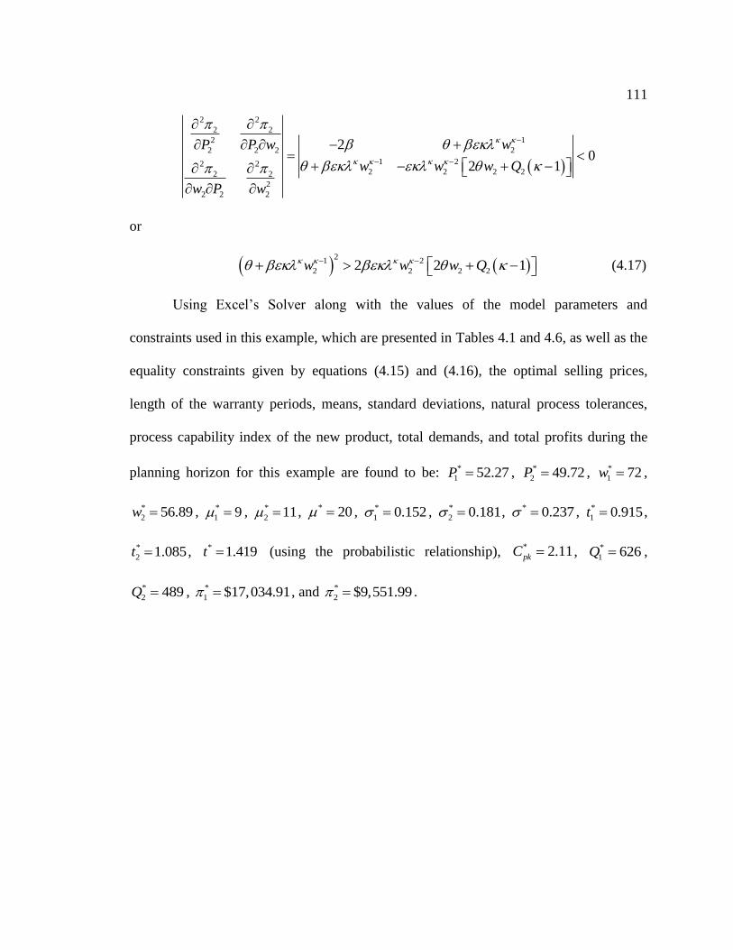
111

2 2

2 2

12

22 2 2

1 22 22 2 2 22 2

2

2 2 2

20

2 1

wP P w

w w w Q

w P w

or

2

1 2

2 2 2 22 2 1w w w Q (4.17)

Using Excel’s Solver along with the values of the model parameters and

constraints used in this example, which are presented in Tables 4.1 and 4.6, as well as the

equality constraints given by equations (4.15) and (4.16), the optimal selling prices,

length of the warranty periods, means, standard deviations, natural process tolerances,

process capability index of the new product, total demands, and total profits during the

planning horizon for this example are found to be: *

1 52.27P , *

2 49.72P , *

1 72w ,

*

2 56.89w , *

1 9 , *

2 11 , * 20 , *

1 0.152 , *

2 0.181 , * 0.237 , *

1 0.915t ,

*

2 1.085t , * 1.419t (using the probabilistic relationship), * 2.11pkC , *

1 626Q ,

*

2 489Q , *

1 $17,034.91 , and *

2 $9,551.99 .

112

The total demand function parameters

1000

25

10

10

5

The manufacturing and warranty costs per item of

the existing product (product 2)

15

100

The scale and shape parameters of the Weibull

lifetime distribution of the existing product

0.005

1.5

The minimum and maximum price values for the

two products

10 60P

20 60P


of the warranty periods of the two products

13 72w

23 72w

The minimum and maximum total demands for

the two products during the planning horizon

10 2000Q

20 2000Q



4.1.4 Example 4: A Dynamic Market Analysis Approach

In this example, unlike the other examples considered so far where the market

analysis approach is static, the selling price and the length of the warranty period are

allowed to vary during the planning horizon. Thus, this example is a case of dynamic

market analysis approach. The model considered here is based on the work by Huang et

al. (2007). It is assumed that the selling price and the length of the warranty period can be

modified every six months during a sixty-month ( 60L ) planning horizon. The

objective function for the integrated parameter and tolerance designs model is to

maximize the total discounted profit over the planning horizon L , which is given by

(Huang et al., 2007):

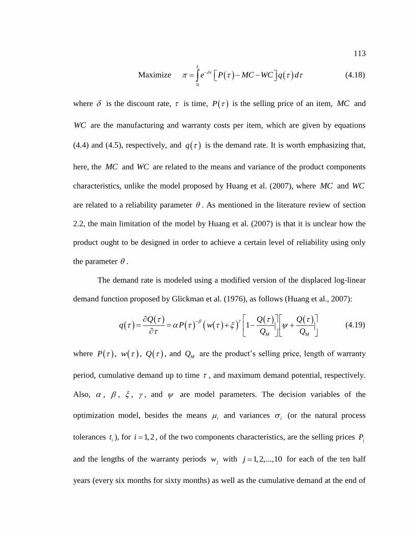
113

Maximize 0

L

e P MC WC q d (4.18)

where is the discount rate, is time, P is the selling price of an item, MC and

WC are the manufacturing and warranty costs per item, which are given by equations

(4.4) and (4.5), respectively, and q is the demand rate. It is worth emphasizing that,

here, the MC and WC are related to the means and variance of the product components

characteristics, unlike the model proposed by Huang et al. (2007), where MC and WC

are related to a reliability parameter . As mentioned in the literature review of section

2.2, the main limitation of the model by Huang et al. (2007) is that it is unclear how the

product ought to be designed in order to achieve a certain level of reliability using only

the parameter .

The demand rate is modeled using a modified version of the displaced log-linear

demand function proposed by Glickman et al. (1976), as follows (Huang et al., 2007):

1M M

Q Q Qq P w

Q Q

(4.19)

where P , w , Q , and MQ are the product’s selling price, length of warranty

period, cumulative demand up to time , and maximum demand potential, respectively.

Also, , , , , and are model parameters. The decision variables of the

optimization model, besides the means i and variances i (or the natural process

tolerances it ), for 1,2i , of the two components characteristics, are the selling prices jP

and the lengths of the warranty periods jw with 1,2,...,10j for each of the ten half

years (every six months for sixty months) as well as the cumulative demand at the end of

114

the planning horizon LQ . The reason for using 60LQ Q as a decision variable is

because q depends on the value of Q , as shown in equation (4.19). Thus, after

finding 60q from equation (4.19), backward induction is used to find all values of

Q using (Huang et al., 2007):

6 6Q Q q (4.20)

for 0,6,12,...,54 with q calculated from equation (4.19), such that, 00Q Q .

The values of the model parameters and constraints used in this example, besides the

ones that are already shown in Table 4.1, are given in Table 4.7.

The discounted rate 0.1

The demand rate function parameters

10,000,000

2.5

0.1

0.3

0.03

The initial demand (added to the model as an

equality constraint) 0 2000Q

The total demand potential 30,000MQ

The minimum and maximum price values for the

ten half years ( 1,2,...,10j ) 0 60jP


of the warranty periods for the ten half years

( 1,2,...,10j )

3 72jw



115

Using Excel’s Solver, the optimal means, standard deviations, natural process

tolerances, and process capability index for this example are found to be: *

1 9 ,

*

2 11, * 20 , *

1 0.175 , *

2 0.208 , * 0.272 , *

1 1.051t , *

2 1.246t , * 1.63t

(using the probabilistic relationship), and * 1.84pkC . Moreover, the optimal selling

prices, lengths of the warranty periods, cumulative demand, and discounted profit for

each of the ten half years are given in Table 4.8.

*P *w

*q *Q *

0 – – – 2000 –

6 31.09 34.54 1285.32 9712 54166.47

12 43.27 52.95 707.78 13959 34146.07

18 49.29 63.02 524.48 17106 17438.24

24 53.41 70.23 407.92 19553 8479.40

30 55.45 72 332.30 21547 4042.84

36 57.09 72 268.07 23155 1887.28

42 58.15 72 218.36 24465 871.61

48 57.50 64.64 182.02 25558 399.08

54 52.38 40.17 161.56 26527 178.29

60 44.29 26.77 162.19 27500 76.65

Table 4.8: The optimal solution for each of the ten half year periods.

4.2 Discussion

Similar to the proposed models of Chapter 3, it is important to note that the

purpose of the integrated parameter and tolerance designs models, which are presented in

116

the examples of section 4.1, is not to serve as comprehensive models for new product

development to be used blindly by designers and practitioners. Instead, the main goal of

these integrated models is to present the viability and flexibility of the general framework

of introducing microeconomic and marketing decisions at the early stages of new product

development. It is left to the designer and practitioner to use the right model elements that

best fit their real-life applications.

In this chapter, besides the new expected utility function given by equation (4.10),

there is no attempt or claim to develop new microeconomic and marketing models. Thus,

it can be noticed from the examples of section 4.1 that the aspects of the integrated

parameter and tolerance models related to microeconomic and marketing modeling, i.e.

demand functions, market structures, equilibrium conditions for the duopoly competition,

etc., follow closely existing models from the microeconomic and marketing literature. A

conscious decision is made not to alter these existing models except when it is necessary

to fit the general framework of the proposed models and to better convey the purpose of

using them. This is to show that there is already a well-established field of study related

to pricing decisions and modeling customer preferences, which leaves no room for poor

representation of customer and market behaviors as it is with the use of the quadratic loss

function. Again, while the idea of the quadratic loss function is a novel one, where it is

used to capture the cost of low product quality, modeling the cost of low product quality

as the cost of warranty and the relatively low product selling price due to low quality is a

more logical and practical approach than trying to list and estimate all possible external

failure costs.

117

The optimal solutions obtained using the integrated parameter and tolerance

designs models of section 4.1 are determined such that the maximum profitability is

achieved while taking virtually all costs, manufacturing capabilities, and market

dynamics as well as the voice of the customer into consideration. As a result, there is no

need to set pkC to an arbitrarily high value, such as 2pkC used by six-sigma

companies, or to impose a lower-bound on pkC as it is done by introducing the constraint

for the natural process tolerance t (equation (3.20)) in the models of Chapter 3.

It is worth mentioning that, even though sensitivity analysis is conducted for two

model parameters from the example of section 4.1.1, full sensitivity analysis is not

pursued for any of the examples of section 4.1. This is because the focus of the examples

is not on drawing specific results and conclusions as much as it is on presenting the

variety of scenarios, challenges, and solution approaches for the integrated parameter and

tolerance designs models with microeconomic and marketing considerations. Despite

that, it is important to note that it is highly recommended in practice to conduct

sensitivity analysis, at least for the main model parameters, since this analysis both

validates the appropriateness of the proposed models and provides additional insights into

the models and their solutions. Obviously, for the examples of section 4.1, sensitivity

analysis can easily be conducted for any model parameter of interest in a similar manner

as it is conducted for the two parameters of the example of section 4.1.1.

118

Chapter 5

Research Contributions and Directions for Future Research

It is concluded from this research that, in order to develop a product that is

competitive and successful in the marketplace, the decisions related to both marketing

and manufacturing operations must be considered simultaneously in an efficient and

optimal manner. This is because the main decisions from both these areas are

interdependent. Setting the selling price and positioning the product in the right market

environment require the knowledge of manufacturing capabilities and costs. On the other

hand, designing the product and the manufacturing processes require the knowledge of

customer preferences and market constraints. Despite that, existing design models from

each of the two fields of marketing and manufacturing lack the required rigor in assessing

the other field’s input to their models. More specifically, it is found that virtually all

existing integrated parameter and tolerance designs models use the quadratic loss

function to capture the voice of the market and customer. The quadratic loss function is

well-known to suffer from its vague definition, simplistic form, and difficult to estimate

proportionality constant. On the other hand, manufacturing and quality costs are grossly

underrepresented in most existing pricing models, where simple functions and

parameters, such as categorical grades and classes for the product quality levels or fixed

and variable costs for the product total costs, are used.

In this research, new integrated parameter and tolerance designs models are

proposed that address the main limitations of existing models and bridge the gap between

119

manufacturing and marketing operations and decisions. The contributions of this research

are highlighted in section 5.1 and the directions for future research are presented in

section 5.2.

5.1 Research Contributions

In this section, the main contributions of this research are presented as follows:

1. One of the most important contributions of this research is proposing

integrated parameter and tolerance designs models that eliminate the

quadratic loss function and replace it with warranty costs. Warranty costs can

be estimated more easily and accurately using warranty and reliability

models, which are well-defined and are based on measurable empirical data.

This greatly simplifies the task of communicating with top management and

making critical decisions about product design and marketing. Moreover, the

warranty and reliability models as well as the manufacturing costs used in the

proposed integrated models are related to product attributes and

specifications, i.e. means and tolerances of all the quality characteristics of

the product and its components, length of the warranty period, process

capability index, etc., thereby establishing a logical and concise framework

for integrating parameter and tolerance designs.

2. The first set of integrated models proposed in this research assumes that the

external failure costs other than warranty costs are negligible. For the cases

where these external failure costs cannot be neglected, a second set of

120

integrated parameter and tolerance designs models are proposed. For these

models, marketing tools, such as pricing models, market structure analysis,

product demand and customer utility functions, etc., are used. These

proposed integrated models are based on the idea that external failure costs

other than warranty costs can be estimated as the increase (decrease) in the

price the customer is willing to pay for the product relative to the amount of

increase (decrease) in product quality. In other words, the opportunity costs

of using low quality products are considered as opposed to actual costs and

losses. Consequently, the benefits of the second set of the proposed

integrated parameter and tolerance designs models is twofold. First, the issue

of the external failure costs other than warranty costs is addressed. Second,

existing pricing and competition models from the microeconomic and

marketing fields are improved by introducing in them better models for the

manufacturing and warranty costs of the product, which are related to

product attributes and specifications.

3. The flexibility of the general framework of the proposed integrated parameter

and tolerance designs models and its applicability to a wide range of

problems are clearly demonstrated using a variety of numerical examples and

solution methodologies. The numerical examples include the cases of linear

and nonlinear relationships between the main quality characteristic of the

product and the quality characteristics of its components as well as the case

of finite manufacturing processes. Moreover, numerical examples for the

cases of static market analysis approach for a general demand function, a

121

monopoly, and a duopoly competition as well as the case of a dynamic

market analysis approach are also considered. In these different numerical

examples, a variety of optimization and analysis techniques, such as

nonlinear programming, integer programming, response surface

methodology, simulation, and sensitivity analysis, are employed to show the

methodology of handling the different design problems.

4. There are several specific contributions that can be mentioned, which are

consequences of the more technical part of this research. These contributions

include:

a. Improving the stack-up constraint for the allowable design tolerance t

of the main product characteristic by relating t to the means and the

natural process tolerances of the product components characteristics

using the process capability index pkC (equation (3.20)). Most existing

integrated parameter and tolerance designs models either fail to

properly include the effects of the means of the components

characteristics in the stack-up constraint for t or simply ignore them

altogether.

b. Proposing a new customer utility function that is related to the product

selling price P , the length of the warranty period w , and the process

capability index pkC . Not only does this new utility function include

more than one metric of product quality, i.e. w and pkC , but also the

quality metrics w and pkC better resonate with the customer when

122

assessing the product quality as opposed to relating product quality

directly to product specifications, such as means and variances of the

quality characteristics of the product and its components. Details about

the formulation of this new utility function are found in section 4.1.2.

5.2 Directions for Future Research

In this section, several directions for future research are suggested as follows:

1. The methodology of implementing and validating the integrated parameter

and tolerance designs models proposed in this dissertation have been shown

using simple and fictitious numerical examples. An area of future research

would be to see how the proposed models perform using real-life problems.

2. The proposed models can be extended and modified to include other issues

that have not been considered, such as fixed costs, inventory costs, quality

inflation, advertisement, cooperation of rival firms, transportation, etc.

3. The product demand and customer utility are represented in the proposed

models using deterministic functions, i.e. the expected demand and expected

utility are used. These functions can probably better represent the customer

and market behaviors by replacing them with stochastic functions that follow

certain probability distributions, as suggested by Lin et al. (2005).

4. In real life problems, the costs of monitoring and maintaining the means of

the quality characteristics at their intended nominal values can be significant.

These costs are not considered in the proposed models. Thus, the proposed

123

models can be modified to include these costs and to allow for some level of

deviation from the optimal values. The implications of these modifications

should be taken into consideration, especially their effects on the reliability

model.

5. Another area of future research is to analyze the model complexity and

compare different optimization algorithms, heuristics, etc., in order to

identify ways to simplify the problem and its solution without sacrificing

real-life representation.

6. In the proposed models, the length of the warranty period is the main metric

used as the signal for product quality to the customer. A direction of future

research can be to study other metrics that affect the customer’s purchasing

decisions and patterns. Product effectiveness, weight, brightness, toxicity,

scent, durability, texture, quietness, etc., are examples of product metrics.

These metrics are likely to vary greatly from one product (or one market) to

another.

7. In order to take full advantage of the proposed models, the Graphic User

Interface (GUI) capabilities of software programs, such as MATLAB, can be

used to program the process of importing and reading data, fitting models,

optimizing, and conducting sensitivity analysis in a user-friendly manner.

This way, the procedure of implementing the proposed models by designers

and practitioners and communicating their results to top management is

greatly simplified.

124

Appendix A

Minitab Output of the Central Composite Design (CCD)

One replication of the Central Composite Design (CCD) generated by Minitab for

the example of section 3.2.2.1 is shown below:

Central Composite Design Factors: 4 Replicates: 1

Base runs: 31 Total runs: 31

Base blocks: 1 Total blocks: 1

Two-level factorial: Full factorial

Cube points: 16

Center points in cube: 7

Axial points: 8

Center points in axial: 0

Alpha: 2

Design Table

Run Blk A B C D

1 1 -1 -1 -1 -1

2 1 1 -1 -1 -1

3 1 -1 1 -1 -1

4 1 1 1 -1 -1

5 1 -1 -1 1 -1

6 1 1 -1 1 -1

7 1 -1 1 1 -1

8 1 1 1 1 -1

9 1 -1 -1 -1 1

10 1 1 -1 -1 1

11 1 -1 1 -1 1

12 1 1 1 -1 1

13 1 -1 -1 1 1

14 1 1 -1 1 1

15 1 -1 1 1 1

16 1 1 1 1 1

17 1 -2 0 0 0

18 1 2 0 0 0

19 1 0 -2 0 0

20 1 0 2 0 0

21 1 0 0 -2 0

22 1 0 0 2 0

23 1 0 0 0 -2

125

24 1 0 0 0 2

25 1 0 0 0 0

26 1 0 0 0 0

27 1 0 0 0 0

28 1 0 0 0 0

29 1 0 0 0 0

30 1 0 0 0 0

31 1 0 0 0 0

126

Appendix B

Cholesky Decomposition of a Two-by-Two Covariance Matrix

Given a covariance matrix that is positive definite, the Cholesky decomposition

is defined as the matrix C such that TCC (Kroese et al., 2011). For a two-by-two

covariance matrix, let:

1 2

3 4

0

0

Ts s a a b

CCs s b c c

(B.1)

Then,

2

1

2

3

2 2

4

s a

s ab

s ab

s b c

(B.2)

Solving for a , b , and c ,

1

2

1

2

24

1

a s

sb

s

sc s

s

(B.3)

Thus, for a covariance matrix given by:

2

1 1 2

2

1 2 2

(B.4)

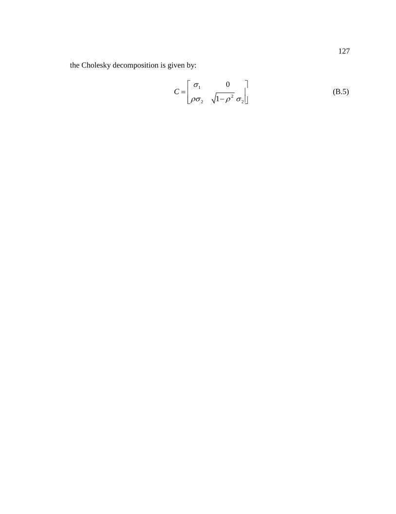
127

the Cholesky decomposition is given by:

1

2

2 2

0

1C

(B.5)

128

Appendix C

Normality Check for 1 2

X X X

In section 3.2.2.2, it is assumed that 1 2X X X is normally distributed so that

sensitivity analysis can be conducted in a straightforward manner as in section 3.2.1.2. In

order to check the appropriateness of the normality assumption, a comparison is made

between random samples that are generated for 1 2X X X , where 1X and 2X have a

joint multivariate normal distribution with a correlation coefficient , and a normally

distributed X with mean and variance 1 2 1 2 and

2 2 2 2 2

2 1 1 2 1 2 1 22 , respectively. Figure C.1 shows the Probability Density

Functions (PDFs) for 1 2X X X and the normally distributed X , where the PDFs are

obtained using histograms of the randomly generated samples for 1 9 , 2 11 ,

1 0.3 , 2 0.3 , and 0.8 (different values for 1 , 2 , 1 , 2 , and were used

to generate the random samples and similar results were obtained). It can be seen from

Figure C.1 that the random sample of 1 2X X X has the appropriate bell-shaped PDF,

which is almost identical in shape to the PDF of the random sample of the normally

distributed X . Moreover, the values of the means and standard deviations of the two

random samples are also very similar.

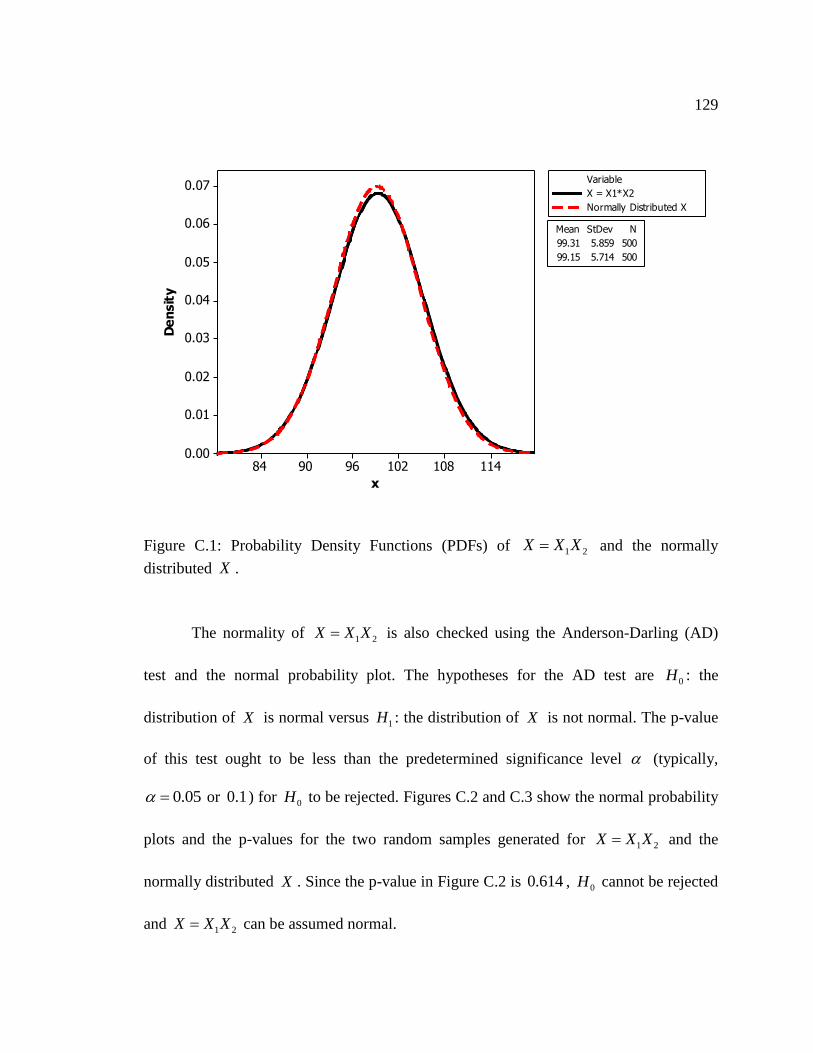
129

114108102969084

0.07

0.06

0.05

0.04

0.03

0.02

0.01

0.00

x

De

nsit

y

99.31 5.859 500

99.15 5.714 500

Mean StDev N

X = X1*X2

Normally Distributed X

Variable

Figure C.1: Probability Density Functions (PDFs) of 1 2X X X and the normally

distributed X .

The normality of 1 2X X X is also checked using the Anderson-Darling (AD)

test and the normal probability plot. The hypotheses for the AD test are 0H : the

distribution of X is normal versus 1H : the distribution of X is not normal. The p-value

of this test ought to be less than the predetermined significance level (typically,

0.05 or 0.1 ) for 0H to be rejected. Figures C.2 and C.3 show the normal probability

plots and the p-values for the two random samples generated for 1 2X X X and the

normally distributed X . Since the p-value in Figure C.2 is 0.614 , 0H cannot be rejected

and 1 2X X X can be assumed normal.

130

1201101009080

99.9

99

95

90

80

70

605040

30

20

10

5

1

0.1

X = X1*X2

Pe

rce

nt

Mean 99.31

StDev 5.859

N 500

AD 0.289

P-Value 0.614

Figure C.2: Normal probability plot for 1 2X X X .

1201101009080

99.9

99

95

90

80

70

605040

30

20

10

5

1

0.1

Normally Distributed X

Pe

rce

nt

Mean 99.15

StDev 5.714

N 500

AD 0.281

P-Value 0.641

Figure C.3: Normal probability plot for the normally distributed X .

131

Bibliography

Bagajewicz, M., “On the Integration of Process and Product Design with

Microeconomics and Finances,” Enpromer 2005, 2nd Mercosur Congress on

Chemical Engineering, 4th Mercosur Congress on Process Systems Engineering,

Rio de Janeiro, Brazil, 2005.

Bagajewicz, M., “On the Role of Microeconomics, Planning, and Finances in Product

Design,” AIChE Journal, 53, 12, 3155-3170, 2007.

Banker, R., I. Khosla, and K. Sinha, “Quality and Competition,” Management Science,

44, 9, 1179-1192, 1998.

Barlow, R. and L. Hunter, “Optimum Preventive Maintenance Policies,” Operations

Research, 8, 1, 90-100, 1960.

Bertrand, J., “Book Review of Theorie Mathematique de la Richesse Sociale and of

Recherches sur les Principes Mathematiques de la Theorie des Richesses,”

Journal des Savants, 67, 499-508.

Blischke, W. and D. Murthy, Product Warranty Handbook, Marcel Dekker, New York,

NY, 1996.

Blue, J., Reliability Functions Incorporating the Mean and the Variance, M.S. Thesis,

Industrial and Manufacturing Engineering, Penn State University, 2001.

Boyes, W. and M. Melvin, Microeconomics, 8th

Edition, South-Western, Mason, OH,

2011.

132

Casella, G. and R. Berger, Statistical Inference, 2nd

Edition, Duxbury Press, Pacific

Grove, CA, 2002.

Chamberlin, E., The Theory of Monopolistic Competition, Harvard University Press,

Cambridge, MA, 1932.

Chandra, M. J., Statistical Quality Control, CRC Press, Boca Raton, FL, 2001.

Chen, C. and W. Chang, “Optimal Design of Expected Lifetime and Warranty Period for

Product with Quality Loss and Inspection Error,” Expert Systems with

Applications, 37, 3521-3526, 2010.

Cho, B., Y. Kim, D. Kimbler, and M. Phillips, “An Integrated Joint Optimization

Procedure for Robust and Tolerance Design,” International Journal of Production

Research, 38, 10, 2309-2325, 2000.

Clements, J., “Process Capability Calculations for Non-normal Calculations,” Quality

Progress, 22, 95-100, 1989.

Cournot, A., Recherches sur les Principes Mathematiques de la Theorie des Richesses,

Hachette, Paris, 1838.

DeCroix, G., “Optimal Warranties, Reliabilities and Prices for Durable Goods in an

Oligopoly,” European Journal of Operational Research, 112, 554-569, 1999.

Deleveaux, V., Analytical Models for Justification of Investment in Continuous Quality

Improvement, Ph.D. Dissertation, Industrial and Manufacturing Engineering, Penn

State University, 1997.

133

Elsayed, E., Reliability Engineering, Addison Wesley Longman, Inc., Reading, MA,

1996.

Feng, C. and A. Kusiak, “Robust Tolerance Design with the Integer Programming

Approach,” Journal of Manufacturing Science and Engineering, 119, 603-610,

1997.

Friedman, J., Oligopoly Theory, Cambridge University Press, Cambridge, UK, 1983.

Glickman, T. and P. Berger, “Optimal Price and Protection Period Decisions for a

Product under Warranty,” Management Science, 22, 1381-1389, 1976.

Hassan, J., External Failure Cost Estimation Using Reliability Models: an Alternative to

Taguchi’s Loss Function, M.S. Thesis, Industrial and Manufacturing Engineering,

Penn State University, 2009.

Hillier, F. and G. Lieberman, Introduction to Operations Research, 8th

Edition, McGraw-

Hill, New York, NY, 2005.

Hotelling H. “Stability in Competition,” Economic Journal, 39, 41-57, 1929.

Hogg, R. and E. Tanis, Probability and Statistical Inference, 7th

Edition, Pearson Prentice

Hall, Upper Saddle River, NJ, 2006.

Huang, H., Z. Liu, and D. Murthy, “Optimal Reliability, Warranty and Price for New

Products,” IIE Transactions, 39, 819-827, 2007.

Jeang, A., “Robust Tolerance Design by Response Surface Methodology,” The

International Journal of Advanced Manufacturing Technology, 15, 399-403,

1999.

134

Jeang, A., “Combined Parameter and Tolerance Design Optimization with Quality and

Cost,” International Journal of Production Research, 39, 5, 923-952, 2001.

Jeang, A., “Simultaneous Parameter and Tolerance Design for an Electronic Circuit via

Computer Simulation and Statistical Optimization,” The International Journal of

Advanced Manufacturing Technology, 21, 1035-1041, 2003.

Jeang, A. and C. Chang, “Combined Robust Parameter and Tolerance Design using

Orthogonal Arrays,” The International Journal of Advanced Manufacturing

Technology, 19, 442-447, 2002a.

Jeang, A. and C. Chang, “Concurrent Optimization of Parameter and Tolerance Design

via Computer Simulation and Statistical Method,” The International Journal of

Advanced Manufacturing Technology, 19, 432-441, 2002b.

Jeyakumar, K. and T. Robert, “Joint Determination of Price, Warranty Length and

Production Quantity for New Products under Free Renewal Warranty Policy,” 4th

International Quality Conference, 105-114, 2010.

Karmarkar, U. and R. Pitbladdo, “Quality, Class, and Competition,” Management

Science, 43, 1, 27-39, 1997.

Kim, Y. and B. Cho, “Economic Considerations on Parameter Design,” Quality and

Reliability International, 16, 501-514, 2000a.

Kim, Y. and B. Cho, “Economic Integration of Design Optimization,” Quality

Engineering, 12, 4, 561-567, 2000b.

135

Kroese, D., T. Taimre, and Z. Botev, Handbook of Monte Carlo Methods, Wiley,

Hoboken, NJ, 2011.

Kuenne, R., Price and Nonprice Rivalry in Oligopoly: The Integrated Battleground, St.

Martin’s Press, New York, NY, 1998.

Ladany, S. and H. Shore, “Profit Maximizing Warranty Period with Sales Expressed by a

Demand Function,” Quality and Reliability Engineering International, 23, 291-

301, 2007.

Lee, H., “The Investment Model in Preventive Maintenance in Multi-Level Production

Systems,” International Journal of Production Economics, 112, 2, 816-828, 2008.

Leemis, L., Reliability: Probabilistic Models and Statistical Methods, 2nd

Edition,

Prentice Hall, Englewood Cliffs, New Jersey, 2009.

Li, W. and C. Wu, “An Integrated Method of Parameter Design and Tolerance Design,”

Quality Engineering, 11, 3, 417-425, 1999.

Lin, P. and L. Shue, “Application of Optimal Control Theory to Product Pricing and

Warranty with Free Replacement under the Influence of Basic Lifetime

Distributions,” Computers and Industrial Engineering, 48, 69-82, 2005.

McCormack, D., I. Harris, A. Huwitz, and P. Spagon, “Capability Indices for Non-

normal Data,” Quality Engineering, 12, 489-495, 2000.

Menezes, M. and I. Currim, “An Approach for Determination of Warranty Length,”

International Journal of Research in Marketing, 9, 177-195, 1992.

136

Miller, R., Economics Today: The Micro View, 13th

Edition, Pearson Addison Wesley,

Boston, MA, 2006.

Monga, A. and M. Zuo, “Optimal System Design Considering Maintenance and

Warranty,” Computers and Operations Research, 25, 9, 691-705, 1998.

Murthy, D., “Product Warranty and Reliability,” Annals of Operations Research, 143,

133-146, (2006).

Nguyen, D. and D. Murthy, “A General Model for Estimating Warranty Costs for

Repairable Products,” IIE Transactions, 16, 4, 379-386, 1984.

Parkinson, D., “The Application of a Robust Design Method to Tolerancing,” Journal of

Mechanical Design, 122, 149-154, 2000.

Puu, T. and I. Sushko, Oligopoly Dynamics: Models and Tools, Springer-Verlag, Berlin,

Germany, 2002.

Sauer, T., Numerical Analysis, Pearson Addison Wesley, Boston, MA, 2006.

Sinha, S. and S. Sarmah, Price and Warranty Competition in a Duopoly Supply Chain, In

T. Choi and T. Cheng (Eds.), Supply Chain Coordination under Uncertainty,

International Handbooks on Information Systems (pp. 281-314), Springer-Velag

Berlin Heidelberg, 2011.

Stackelberg, H., Marktform und Gleichgewicht, Springer, Vienna, Austria, 1934.

Taguchi, G., and D. Clausing, “Robust Quality,” Harvard Business Review, 68, 1, 65-75,

1990.

137

Teng, J. and G. Thompson, “Optimal Strategies for General Price-Quality Decision

Models of New Products with Learning Production Costs,” European Journal of

Operational Research, 93, 476-489, 1996.

Voros, J., “The Dynamics of Price, Quality and Productivity Improvement Decision,”

European Journal of Operational Research, 170, 809-823, 2006.

Whitnack, C., A. Heller, and M. Bagajewicz, “A Microeconomics-Based Approach to

Product Design under Uncertainty,” 18th European Symposium on Computer

Aided Process Engineering, 181-186, 2008.

Wu, C., C. Chou, and C. Huang, “Optimal Price, Warranty Length and Production Rate

for Free Replacement Policy in the Static Demand Market,” Omega – The

International Journal of Management Science, 37, 29-39, 2009.

Wu, C., Z. Chen, and G. Tang, “Component Tolerance Design for Minimum Quality

Loss and Manufacturing Cost,” Computers in Industry, 35, 223-232, 1998.

Wu, C., P. Lin, and C. Chou, “Determination of Price and Warranty Length for a Normal

Lifetime Distributed Product,” International Journal of Production Economics,

102, 95-107, 2006.

Zhang, J., S. Li, N. Bao, G. Zhang, D. Xue, and P. Gu, “A Robust Design Approach to

Determination of Tolerances of Mechanical Products,” CIRP Annals –

Manufacturing Technology, 59, 195-198, 2010.

138

Zhang, Y., An Alternative to Taguchi’s Loss Function Using Capability Index, M.Eng.

Scholarly Paper, Industrial and Manufacturing Engineering, Penn State

University, 2006.

Zhang, Z., X. Bai, and Z. He, “Construction of Six Sigma Tolerance Design Model Based

on Dual Response Surface Methodology,” Proceedings of the 7th World Congress

on Intelligent Control and Automation, Chongqing, China, 2008.

Vita

Jawad S. Hassan

Jawad S. Hassan is currently in the process of finishing his dual-title Ph.D. degree in

Industrial Engineering and Operations Research with a minor in Statistics from The

Pennsylvania State University. After graduation, he will join the department of Industrial

and Management Systems Engineering at Kuwait University as an assistant professor.

Jawad received his B.S. and M.S. degrees in Mechanical Engineering from The

Pennsylvania State University in 2003 and 2005, respectively. His M.S. thesis is titled:

“Numerical Study of the Effect of High Free-Stream Turbulence on Flat-Plate Film

Cooling Effectiveness using FLUENT”, and it was under the supervision of Professor

Savas Yavuzkurt. With a teaching assistantship from the Mechanical and Nuclear

Engineering Department at The Pennsylvania State University and after spending a year

in its Mechanical Engineering Ph.D. program, Jawad was offered a full scholarship from

Kuwait University to pursue his M.S. and Ph.D. degrees in Industrial Engineering. He

received his dual-title M.S. degree in Industrial Engineering and Operations Research

with a Quality Engineering option from the Pennsylvania State University in 2009. His

second M.S. thesis is titled: “External Failure Cost Estimation using Reliability models:

an Alternative to Taguchi’s Loss Function”, and it was under the supervision of Professor

M. Jeya Chandra.

integrated models and methodologies for parameter …

Documents