integrating financial statement modeling and sales ... · integrating financial statement modeling...

Integrating Financial Statement Modeling and Sales Forecasting Using EViews

John T. Cuddington

Colorado School of Mines

Irina Khindanova University of Denver

This paper shows how to integrate pro forma financial statement analysis and sales forecasting using the EViews software package. The integration enables us to use the forecast of future sales and the associated standard errors to carry out an empirically-based Monte Carlo simulation of the future paths of all income and balance sheet items in the pro forma statements. This provides useful additional information to the financial analyst. Not only does he/she obtain expected future values for the various pro forma statement items, there are also confidence intervals that can be used to assess the uncertainty of the financial forecasts. INTRODUCTION

In most business school programs students are exposed to financial statement modeling1 and to introductory statistical and econometric methods, including forecasting (especially – sales forecasting).2 However, there is seldom an attempt to integrate them within a unified framework. The objectives of this paper are to show how such integration can be done using the EViews econometrics package.

The paper begins by showing how to implement a simple sales-driven model of financial statements using EViews, rather than Excel. Our illustration uses a model from Simon Bennninga’s popular Financial Modeling textbook (2008, Ch.3). The EViews model is transparent and easy to audit and debug because the financial equations are written out explicitly in a MODEL object in EViews rather than being embedded in Excel’s cell formulas. Although the steps can be carried out using EViews’ graphical user interface, we provide a well-documented EViews program to automate the entire exercise. Thus, it should be easy for other researchers to replicate and extend the EViews model.

Next, we calibrate our EViews version of the Benninga model using historical data for Home Depot, then generate pro forma statements over the 2011-2016 time span. This projection exercise like Benninga’s is deterministic not stochastic; i.e. sources of uncertainty are not explicitly modeled. To develop a stochastic generalization of the model, we estimate a simple univariate forecasting equation for Home Depot sales. The uncertainty regarding future sales captured by the standard error of the forecast in future years is used to ‘drive’ stochastic simulation of the entire pro forma statement model where all of the items depend directly or indirectly (via the model’s ratio assumptions and accounting identities) on future sales.

100 Journal of Applied Business and Economics vol. 12(6) 2011

By integrating sales forecasting and the financial statement model we create an empirically-based stochastic generalization of the model. The stochastic model provides a wealth of useful additional information to the financial analyst. Not only does she obtain expected future values for the various pro forma statement variables, but also the corresponding confidence intervals that can be used to assess uncertainty of the financial forecasts. We illustrate the stochastic model output with an analysis of projected sales, profits, cash balances, and outstanding debt.

Although our estimated sales equation is a simple one for illustrative purposes, the procedures outlined in this paper can be implemented with any sales forecasting equation one prefers. It may be a single equation (univariate or reduced form) or one equation in a multi-equation model – be it a vector autoregression (VAR) or structural model. Indeed, with the latter, it is straightforward to introduce several sources of uncertainty, while correctly capturing interactions among the forecasted variables. Confidence intervals would then reflect the error variances in all equations as well as their covariances.

The remainder of the paper is structured as follows. The second section describes an EViews implementation of a simple pro forma statement model from Benninga, 2008. The third section shows how to calibrate and simulate the EViews version of the financial statement model using data for Home Depot. The fourth section develops an illustrative sales forecasting equation. The fifth section explains how to integrate sales forecasting and pro forma models in order to carry out empirically-based stochastic simulation of Home Depot’s financial statements. The sixth section summarizes our findings. PRO FORMA STATEMENT MODELING IN EVIEWS

Benninga (2008, Ch.3) introduces a series of sales-driven Excel models for financial statements.3 In this section, we describe the EViews implementation of his second model. In this model, as long as cash balances remain positive, CASH (which equals cash and marketable securities) is the plug4 and paid-in capital and outstanding long-term debt remain constant (by rolling over any maturing debt). In situations where there is a ‘run down’ in CASH, however, it is assumed that the firm will issue new debt as needed in order to prevent CASH from going negative. Thus, DEBT, in effect, becomes the plug when CASH drops to zero. (It would be straightforward and more realistic to set a minimum CASH threshold at a positive number rather than zero.)

Benninga sets up the model with a set of hypothesized initial figures for the income statement and balance sheet items shown in Table 1. In real-world applications, these figures would be taken from actual financial statements. For ease of reference, we have added our chosen EViews series names in the left-most column of Table 1.

Benninga lays out a simple set of equations and identities to describe the interrelationships among the income statement and balance sheet variables at each future date. These equations are shown in Table 2. Note that the sales growth rate is assumed to be constant (at 20%) over time. The model is ‘sales driven’ in the sense that several key variables are proportional to sales: Cost of Goods Sold, Other Current Assets, Net Fixed Assets, and Current Liabilities. As described above, CASH is the plug with DEBT unchanged as long as CASH is positive. Using the balance sheet identity, therefore, we can write CASH as:

min[0, ( 1) ]CASH CL DEBT EQUITY OCA NFA= + − + − −

where DEBT(-1) denotes debt in the previous period. OCA is Other Current Assets, NFA is Net Fixed Assets, CL is Current Liabilities, and EQUITY= CAPITAL+ACC_EARNINGS. See Table 1 for all variable definitions. When CASH hits zero, however, DEBT becomes the plug. Thus,5

]),1(max[ EQUITYCLNFAOCADEBTDEBT −−+−= .

Journal of Applied Business and Economics vol. 12(6) 2011 101

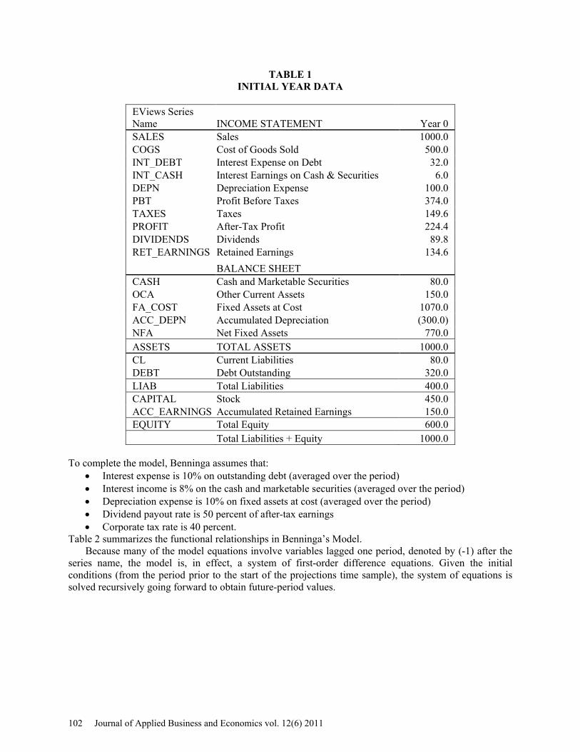
TABLE 1 INITIAL YEAR DATA

EViews Series Name INCOME STATEMENT Year 0 SALES Sales 1000.0 COGS Cost of Goods Sold 500.0 INT_DEBT Interest Expense on Debt 32.0 INT_CASH Interest Earnings on Cash & Securities 6.0 DEPN Depreciation Expense 100.0 PBT Profit Before Taxes 374.0 TAXES Taxes 149.6 PROFIT After-Tax Profit 224.4 DIVIDENDS Dividends 89.8 RET_EARNINGS Retained Earnings 134.6 BALANCE SHEET CASH Cash and Marketable Securities 80.0 OCA Other Current Assets 150.0 FA_COST Fixed Assets at Cost 1070.0 ACC_DEPN Accumulated Depreciation (300.0) NFA Net Fixed Assets 770.0 ASSETS TOTAL ASSETS 1000.0 CL Current Liabilities 80.0 DEBT Debt Outstanding 320.0 LIAB Total Liabilities 400.0 CAPITAL Stock 450.0 ACC_EARNINGS Accumulated Retained Earnings 150.0 EQUITY Total Equity 600.0 Total Liabilities + Equity 1000.0

To complete the model, Benninga assumes that:

• Interest expense is 10% on outstanding debt (averaged over the period) • Interest income is 8% on the cash and marketable securities (averaged over the period) • Depreciation expense is 10% on fixed assets at cost (averaged over the period) • Dividend payout rate is 50 percent of after-tax earnings • Corporate tax rate is 40 percent.

Table 2 summarizes the functional relationships in Benninga’s Model. Because many of the model equations involve variables lagged one period, denoted by (-1) after the

series name, the model is, in effect, a system of first-order difference equations. Given the initial conditions (from the period prior to the start of the projections time sample), the system of equations is solved recursively going forward to obtain future-period values.


TABLE 2 FORMULAS FOR PRO-FORMA FINANCIAL STATEMENTS

Formula for Subsequent Periods Assumptions SALES = SALES(-1)*1.20 Constant Sales growth rate COGS = 0.50*SALES Sales Driven INT_DEBT = .10*(DEBT+DEBT(-1))/2 Given percentage INT_CASH = .08*(CASH+CASH(-1))/2 Given percentage DEPN = .10*(FA_COST+FA_COST(-1))/2 Given percentage PBT = SALES-COGS - INT_DEBT + INT_CASH - DEPN Identity TAXES = .40*PBT Given percentage PROFIT = PBT – TAXES Identity DIVIDENDS = .50*PROFIT Given percentage RET_EARNINGS = PROFIT – DIVIDENDS Identity CASH = CL+DEBT(-1)+EQUITY- OCA + NFA if positive = 0, otherwise The "Plug" OCA = .20*SALES Sales Driven FA_COST = NFA + ACC_DEPN Identity ACC_DEPN = ACC_DEPN(-1) + DEPN Identity NFA = .80*SALES Sales Driven ASSETS = CASH + OCA + NFA Identity CL = .08*SALES Sales Driven; DEBT = DEBT(-1) if CASH ≥ 0 = OCA + NFA - CL – EQUITY otherwise

Debt increases if needed to prevent CASH<0

LIAB = CL + DEBT Identity CAPITAL = CAPITAL(-1) Stock remains constant ACC_EARNINGS = ACC_EARNINGS(-1) + RET_EARNINGS Identity EQUITY = CAPITAL + ACC_EARNINGS Identity

The Benninga model is straightforward to implement and solve using EViews. The steps, which can

be carried out using the user-friendly graphical interface or using an EViews program (see Appendix), are:

(1) Create an EViews workfile with annual frequency and a range that spans the historical data and the desired forecast or projection interval (say, five years). For the Benninga example, we use an undated (rather than annual) EViews workfile with six periods, one for the initial period of data (or initial conditions) and five for the pro forma projections.

(2) Import the income and balance sheet data from Excel file. Be sure to label each series in the Excel file before importing into EViews.

(3) Declare a MODEL object and append all of the model equations, as summarized in Table 2 above.

(4) Solve the model and create two GROUPS with the income statement series and the balance sheet series in order to show the model ‘solutions’ for future periods. If desired, these pro forma statements can be exported to an Excel file for ‘beautification.’ Alternatively, this can be done by creating and formatting a TABLE object within EViews.

The program can easily be adapted for annual, quarterly, or monthly frequencies. Figure 1 shows the generated EViews workfile, which contains series with the initial year data, the Model object named


“model2”, the model solution series with an extension “_0” added to the end of the names, and the income statement and balance sheet tables.

FIGURE 1 EVIEWS WORKFILE FOR BENNINGA’S MODEL

Figure 2 shows the equations as entered into the EViews MODEL object following the Table 2 structure. One of equations constructs a dummy variable (DUM) to determine the sign of CASH balances. When CASH is positive, it is the plug. If CASH can become negative, it is constrained to equal zero and DEBT increases.


FIGURE 2 BENNINGA’S MODEL IN THE EVIEWS MODEL OBJECT

' Income Statement SALES = 1.20 * SALES(-1) COGS = 0.50 * SALES INT_DEBT = (DEBT(-1) + DEBT) / 2 * 0.10 INT_CASH = (CASH(-1) + CASH) / 2 * 0.08 PBT = SALES - COGS - INT_DEBT + INT_CASH - DEPN TAXES = 0.40 * PBT PROFIT = PBT - TAXES DIVIDENDS = 0.50 * PROFIT RET_EARNINGS = PROFIT - DIVIDENDS ' Balance Sheet ' create a dummy variable that is 1 if CASH would be negative in the absence of additional debt, and zero otherwise. ' Using EViews syntax, everything after the equal sign is treated as a logical condition. If it holds, DUM is 1; zero otherwise. DUM = - OCA - NFA + CL + DEBT(-1) + EQUITY < 0 ' define CASH as the balance sheet plug, if positive, and ZERO otherwise by creative use of the dummy: CASH = (- OCA - NFA + CL + DEBT(-1) + EQUITY) * (1 - DUM) OCA = 0.20 * SALES NFA = 0.80 * SALES DEPN = 0.10 * (FA_COST(-1) + FA_COST) / 2 ACC_DEPN = ACC_DEPN(-1) + DEPN FA_COST = NFA + ACC_DEPN ASSETS = CASH + OCA + NFA CL = 0.08 * SALES ' when DUM=1, cash is negative, so DEBT is the plug; ' when DUM=0, cash is positive, so debt is unchanged from the previous period DEBT = (OCA + NFA - CL - EQUITY) * DUM + DEBT(-1) * (1 - DUM) LIAB = DEBT + CL CAPITAL = CAPITAL(-1) ACC_EARNINGS = ACC_EARNINGS (-1) + RET_EARNINGS EQUITY = CAPITAL + ACC_EARNINGS


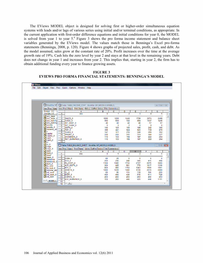
The EViews MODEL object is designed for solving first or higher-order simultaneous equation systems with leads and/or lags of various series using initial and/or terminal conditions, as appropriate. In the current application with first-order difference equations and initial conditions for year 0, the MODEL is solved from year 1 to year 5.6 Figure 3 shows the pro forma income statement and balance sheet variables generated by the EViews model. The values match those in Benninga’s Excel pro-forma statements (Benninga, 2008, p. 120). Figure 4 shows graphs of projected sales, profit, cash, and debt. As the model assumed, sales grow at the constant rate of 20%. Profit increases over the time at the average growth rate of 19%. Cash hits the zero level by year 2 and stays at that level in the remaining years. Debt does not change in year 1 and increases from year 2. This implies that, starting in year 2, the firm has to obtain additional funding every year to finance growing assets.

FIGURE 3 EVIEWS PRO FORMA FINANCIAL STATEMENTS: BENNINGA’S MODEL


FIGURE 4 PROJECTED SALES, PROFIT, CASH, AND DEBT

HOME DEPOT PRO FORMA STATEMENT MODELING IN EVIEWS

In this section we show how to calibrate and solve the EViews version of the financial statement model using historical data for Home Depot.

Based on the financial statements for the last five years, 2006-2010, the following ratios and rates were obtained:7

• sales growth rate = -1.38%, the average over 2006-2010 • COGS/Sales ratio = 89%, the average over 2006-2010 • interest rate on debt = 7%, the 2010 estimate • interest rate earned on cash and cash equivalents = 1%, the 2010 estimate • tax rate = 36%, the average over 2006-2010 • dividend payout ratio = 58%, the 2010 estimate; the average dividend payout ratio over 2006-

2010 was 36% • OCA/Sales ratio = 18% • NFA/Sales ratio = 34% • depreciation rate = 5% • CL/Sales ratio = 16%.

Using these parameter values and starting values for 2010, we solved the EViews financial model for the next six years, 2011-2016.8 Figure 5 shows the initial and simulated balance sheets and income statements for Home Depot. Our analysis of the simulation results focuses on projections of four key items: SALES (model’s “driver”), PROFIT (the income statement bottom line item), CASH (model’s main plug) and DEBT (model’s ancillary plug). Figure 6 presents graphs of these variables. The simulations were based on the assumption that SALES will decline over the projection period of 2011-2016. The model predicts that PROFIT will increase in 2011 but will decline thereafter. As SALES decline, so does cost of goods sold (COGS), TAXES, other current assets (OCA), net fixed assets (NFA), etc. As a result (and given the Home Depot parameter assumptions above), CASH is projected to rise over time! Hence, DEBT stays constant at the 2010 level.


FIGURE 5 HOME DEPOT PRO FORMA STATEMENTS -- SALES DECLINE SCENARIO


FIGURE 6 PROJECTED SALES, PROFIT, CASH, AND DEBT FOR HOME DEPOT:

SALES DECLINE SCENARIO

For comparison, we run the Home Depot model simulations assuming sales increase at the constant

rate of 2.3%.9 The resulting graphs of SALES, PROFIT, CASH, and DEBT are shown in Figure 7. The increasing sales scenario shows that PROFIT will rise in 2011 by about 17% and from 2012 will grow at the declining rates hovering under 1%. The CASH balances are expected to increase to $11.4 billion by 2016, what is lower than the 2016 projection for CASH ($15.5 billion) under the sales decline scenario. The DEBT level is not expected to change.

The Home Depot cash projections in both the sales decline and sales increase scenarios show that the sales-driven model might produce ever increasing cash. That’s not the always the case. The results are, of course, sensitive to the parameter assumption. For example, if we assume that sales increase at 2.3% and change only the NFA/SALES ratio assumption from 34% to 60%, then the model shows that CASH will decline from the 2010 level of $1,421 million to zero in the first projection year 2011 and will stay at the zero level afterwards.


FIGURE 7 PROJECTED SALES, PROFIT, CASH, AND DEBT FOR HOME DEPOT:

SALES INCREASE SCENARIO

The Home Depot model in this section supposes that sales grow at the constant rate. In the next

section we forecast sales assuming the variable growth. THE SALES FORECASTING EQUATION

This section summarizes the estimation of a simple univariate sales forecasting equation for Home Depot. This equation will be incorporated into the EViews model of pro forma statements in the next section.

Figure 8 shows the time plots of sales (on a log scale) and the sales growth rates from 1986 through 2010. Sales growth has declined from a rather spectacular 62% rate in 1986 to sharply negative growth in 2008-2010 (-15%, -8%, and -7%, respectively).


FIGURE 8 HOME DEPOT SALES IN 1985-2010

The negative growth rates are undoubtedly due, at least in part, to the U.S. recession and worldwide

slowdown in 2008-2009, but the declining growth rates prior to that leave concern about longer term prospects. In this situation, univariate forecasting techniques may not provide especially accurate forecasts. Multivariate approaches may produce superior results. This, however, is not of particular importance here as our objective is to illustrate how forecasting equations – whether univariate or multivariate, single equation or multiple-equations systems – can be used to carry out empirically based stochastic simulations using EViews. Our estimated sales equation is a linear time trend model10 for the continuously compounded annual SALES growth rate (equal to the first difference of the natural logarithm of SALES): ttt tSALESLOGSALESLOG ε+−=− − 019215.0450985.0)()( 1 , (1) where LOG denotes the natural logarithm function, t is time, εt is the residual term,

))(()()( 1 SALESLOGDSALESLOGSALESLOG tt =− − in the EViews notations. The estimation output results are displayed in Table 3. The equation is estimated with Newey-West robust standard

TABLE 3 ESTIMATED SALES EQUATION

Dependent Variable: D(LOG(SALES)) Method: Least Squares Date: 02/20/11 Time: 21:49 Sample (adjusted): 1986 2010 Included observations: 25 after adjustments Newey-West HAC Standard Errors & Covariance (lag truncation=2) Coefficient Std. Error t-Statistic Prob. C 0.450985 0.023881 18.88463 0.0000 @TREND -0.019215 0.002208 -8.702750 0.0000 R-squared 0.866251 Mean dependent var 0.201194 Adjusted R-squared 0.860436 S.D. dependent var 0.151942 S.E. of regression 0.056763 Akaike info criterion -2.823245 Sum squared resid 0.074107 Schwarz criterion -2.725735 Log likelihood 37.29056 Hannan-Quinn criter. -2.796200 F-statistic 148.9637 Durbin-Watson stat 1.484233 Prob(F-statistic) 0.000000


errors. The t-statistics, derived with these standard errors, are above two, what shows that the intercept term and the time coefficient are statistically significant. The adjusted R2 value (.86) is high. It indicates that model (1) provides a good fit. Graphs of actual and fitted values of the dependent variable D(LOG(SALES)) and graphs of the residuals are shown in Figure 9. The correlogram of the residuals is flat, suggesting an absence of serial correlation. The Breusch-Godfrey LM test of the null hypothesis that there is no first or second-order correlation is not rejected (χ2=1.41).

FIGURE 9 SALES EQUATION RESIDUALS

INTEGRATING THE SALES FORECAST AND THE PRO FORMA STATEMENT MODEL

This section describes integration of the sales forecast and the financial statement model. First, we link the sales forecasting equation (estimated in the fourth section) with the model of financial statements (explained in the third section). Next, we use the stochastic simulation features in the EViews MODEL to forecast sales and all of the other income and balance sheet items into the future. Through Monte Carlo simulation methods (using 10,000 stochastic repetitions), the means and confidence bands for each variable at each future dates are obtained. We show the results for PROFIT and CASH balances.

In order to integrate the sales forecast and the pro forma statement model, we replace the constant sales growth equation in the deterministic version of the Home Depot model (SALES = 0.9862*SALES(-1)) with a link to the estimated sales equation in the workfile (:SALES_EQ). This link is a basis of stochastic simulations of pro forma statements.

We wrote a program that automates the EViews implementation of both deterministic and stochastic models for Home Depot. The program creates an annual frequency workfile with the time range 1985-2016, imports the balance sheet and the income statement for the initial year - 2010, creates and solves the deterministic model for 2011-2016, shows the projected income statement and balance sheet, and exports them into Excel files. Next, the program integrates sales forecasting and the pro forma statement model.11 The steps are:


• Copy the EViews page with Benninga's model of financial statements for Home Depot to a new page within the workfile. This new page will integrate sales forecasts and pro forma financial statements

• Load a page with an estimated sales equation • Make the integrating page the active page • Copy the sales equation to the integrating page • Create a stochastic model, which links sales forecasting equation with the earlier deterministic

model of financial statements • Solve the stochastic model from 2011 to 2016. Figure 10 shows the created EViews workfile with pages for solving the deterministic model

(MODEL2_HD), for integrating sales forecasts and the pro forma statement model (SALES_F_STMNTS), and estimating the sales equation. The SALES_F_STMNTS page is active.

FIGURE 10 EVIEWS WORKFILE FOR INTEGRATING SALES FORECASTS AND PRO FORMA

STATEMENT MODEL


It contains the following items: • series with the initial year data • two Model objects (“model2” – deterministic model; “model2s” – stochastic model) • the deterministic model solution series with an extension ”_0” added to the end of the

names • the stochastic model solution series with four different name extensions:

o “_0h” – upper forecasts, the upper 95% confidence bounds o “_0l” – lower forecasts, the lower 95% confidence bounds o “_0m” – mean forecasts o “_0s” – standard deviations of the mean forecasts

Solving the model with the incorporated sales equation allows us to easily produce the future SALES forecasts and their 95% (or other user selected) confidence intervals, shown in Figure 11. The model projects that SALES will decline from $66,176 million in 2010 to $37,491 million in 2016.

FIGURE 11 UNIVARIATE SALES FORECASTS FOR HOME DEPOT

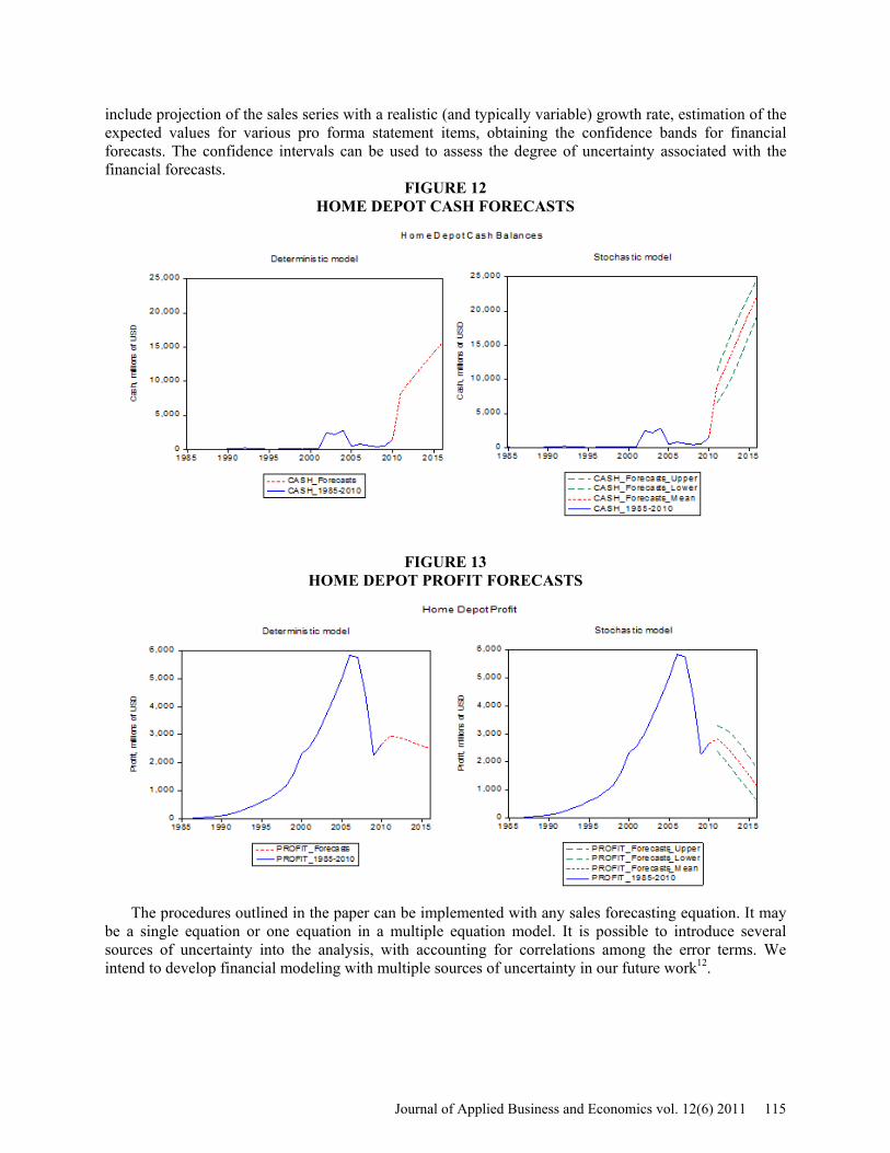
We depict CASH and PROFIT forecasts generated by the stochastic model in Figures 12 and 13.

Comparing to the deterministic model forecasts (derived under the assumption of the constant sales growth rate = -1.38%), the stochastic model projects a steeper increase of the CASH balances and a faster decline in PROFIT. CONCLUSIONS

This paper demonstrates how to integrate pro forma financial statements with sales forecasting. The integration was performed in four steps: (i) modeling of financial statements in the EViews; (ii) estimation of a sales forecasting equation; (iii) linkage of the sales forecasting equation and the EViews model of financial statements; (iv) forecasting sales and other items in the pro forma statements and constructing confidence intervals for those forecasts.

The illustration developed in this paper shows that EViews modeling of financial statements has the benefit of being more transparent and easier to audit and debug than the same financial model implemented in the Excel spreadsheet program. Advantages of the use of sales forecasting equation


include projection of the sales series with a realistic (and typically variable) growth rate, estimation of the expected values for various pro forma statement items, obtaining the confidence bands for financial forecasts. The confidence intervals can be used to assess the degree of uncertainty associated with the financial forecasts.

FIGURE 12 HOME DEPOT CASH FORECASTS

FIGURE 13 HOME DEPOT PROFIT FORECASTS

The procedures outlined in the paper can be implemented with any sales forecasting equation. It may

be a single equation or one equation in a multiple equation model. It is possible to introduce several sources of uncertainty into the analysis, with accounting for correlations among the error terms. We intend to develop financial modeling with multiple sources of uncertainty in our future work12.


ENDNOTES

1. See Benninga (2008), Charnes (2007), Holden (2009), Sengupta (2007), Winston (2008) for detailed examples of financial statement modeling.

2. See Diebold (2007) for a representative discussion of forecasting methods. 3. The sales-driven models assume that the key variables in financial statements are functions of

sales. 4. The plug guarantees that assets are equal to liabilities and equity. 5. In EViews, we use a dummy variable rather than the min and max functions shown here to

determine whether CASH is positive or not. This dummy is then used to determine whether CASH or DEBT, in effect, becomes the plug in any given year.

6. The model can be solved forward for as many periods as the analyst is interested in. 7. The Home Depot financial statements were downloaded from the Mergent Online database. 8. The EViews program for solving the Home Depot model is available at

http://inside.mines.edu/~jcudding/. 9. This is Home Depot’s estimate for the fiscal year ending on January 31, 2011, as reported by

Associated Press on December 8, 2010. 10. We also considered quadratic time trend terms and specifications that assumed two rather than

one unit roots. But they proved to be inferior to the specification reported. 11. The EViews program for integrating sales forecasting and financial statement modeling is

available at http://inside.mines.edu/~jcudding/. 12. Aljihrish et al (2011) are considering multiple sources of uncertainty for projecting Newmont

Mining Corporation’s financial variables.

REFERENCES Aljihrish A., Anouti Y., Cuddington J.T.,, Curado M. & Everett B. (2011). An Integrated Approach to Corporate Financial Planning: The Case of Newmont Mining Corporation. Colorado School of Mines working paper. Diebold, F. X. (2007), Elements of Forecasting. Fourth Edition, South-Western College Publishing Co. Benninga, S. (2008), Financial Modeling. Third Edition, Cambridge, MA: MIT Press. Charnes, J. (2007), Financial Modeling with Crystal Ball and Excel, Hoboken, New Jersey: John Wiley &Sons, Inc. Holden, C. W. (2009), Excel Modeling and Estimation in the Fundamentals of Corporate Finance. Third Edition, Upper Saddle River, New Jersey: Pearson Education, Inc., Person Prentice Hall. Sengupta, C. (2010), Financial Analysis and Modeling Using Excel and VBA. Second Edition, Hoboken, New Jersey: John Wiley &Sons, Inc. Winston, W. (2008), Financial Models Using Simulation and Optimization. Third Edition, Ithaca, New York: Palisade Corporation.


http://inside.mines.edu/~jcudding/�

http://inside.mines.edu/~jcudding/�

APPENDIX

EVIEWS PROGRAM FOR RUNNING BENNINGA’S MODEL ' ================================================= ' 06/05/11 IK JC ' This program implements Benninga's second model of financial statements (Model 2) in EViews ' The model is described in Benninga (2008, Ch. 3) ' Model 2 assumptions: ' (i) Cash and marketable securities is the plug ' (ii) No negative cash balances ' (iii) Debt increases if CA + NFA > CL + Debt(-1) + Accumulated Retained Earnings ' Initial year: 0 ' Projected years: 1-6 ' The program steps: ' 1. Create an annual WORKFILE ' 2. Import the balance sheet and income statement for the initial year - year 0 ' 3. Create and solve Benninga's model of financial statements (Model 2) to generate pro forma statements ' 4. Export the generated financial statements into Excel files. ' 5. Show the generated income statement and balance sheet ' ================================================== ‘ Set default directory where Excel data input files are located CD “c:\jc_1\jc120910” ' 1. Create an undated WORKFILE ' the created workfile will contain a page named (Benninga) Model2 WFCREATE(PAGE = "Model2") MY_WORK U 0 5 ' 2. Import the balance sheet and income statement for the initial year - year 0 SMPL @first @first READ(B2,T) BS_Model2_year0.XLS 10 READ(B2,T) IS_Model2_year0.XLS 10 ' 3. Create and solve Benninga's model of financial statements (Model 2) to generate pro forma statements ' Declare model object named MODEL2 MODEL MODEL2 ' Declare a string and append to the model object as a comment line %Z = " ' Income Statement " MODEL2.APPEND {%Z} ' Add/append the income statement equations to Model 2


' The sales growth rate = 20% MODEL2.APPEND SALES = 1.20*SALES(-1) ' COGS/Sales ratio = 50% MODEL2.APPEND COGS = 0.50 * SALES ' interest rate on debt = 10% MODEL2.APPEND INT_DEBT = (DEBT(-1) + DEBT)/2 * 0.10 ' interest rate earned on cash and cash equivalents = 8% MODEL2.APPEND INT_CASH = (CASH(-1) + CASH)/2 * 0.08 ' Profit Before Taxes MODEL2.APPEND PBT = SALES - COGS - INT_DEBT + INT_CASH - DEPN ' tax rate = 40% MODEL2.APPEND TAXES = 0.40 * PBT MODEL2.APPEND PROFIT = PBT - TAXES 'the dividend payout ratio = 50% MODEL2.APPEND DIVIDENDS = 0.50 * PROFIT MODEL2.APPEND RET_EARNINGS = PROFIT - DIVIDENDS ' Declare a string and append to the model object as a comment line %Z = " ' Balance Sheet " MODEL2.APPEND {%Z} 'Add the balance sheet equations to Model 2 %Z = " ' create a dummy variable that is 1 if CASH would be negative in the absence of additional debt, and zero otherwise. " MODEL2.APPEND {%Z} %Z = " ' Using EViews syntax, everything after the equal sign is treated as a logical condition. If it holds, DUM is 1; zero otherwise. " MODEL2.APPEND {%Z} MODEL2.APPEND DUM = - OCA - NFA + CL + DEBT(-1) + EQUITY < 0 %Z = " ' define CASH as the balance sheet plug, if positive, and ZERO otherwise by creative use of the dummy: " MODEL2.APPEND {%Z} MODEL2.APPEND CASH = (- OCA - NFA + CL + DEBT(-1) + EQUITY) * (1 - DUM) ' OCA/Sales ratio = 20% MODEL2.APPEND OCA = 0.20 * SALES


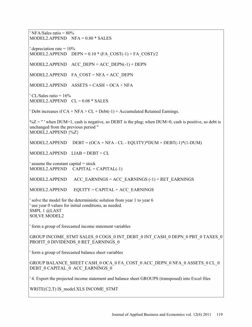
' NFA/Sales ratio = 80% MODEL2.APPEND NFA = 0.80 * SALES ' depreciation rate = 10% MODEL2.APPEND DEPN = 0.10 * (FA_COST(-1) + FA_COST)/2 MODEL2.APPEND ACC_DEPN = ACC_DEPN(-1) + DEPN MODEL2.APPEND FA_COST = NFA + ACC_DEPN MODEL2.APPEND ASSETS = CASH + OCA + NFA ' CL/Sales ratio = 16% MODEL2.APPEND CL = 0.08 * SALES ' Debt increases if CA + NFA > CL + Debt(-1) + Accumulated Retained Earnings. %Z = " ' when DUM=1, cash is negative, so DEBT is the plug; when DUM=0, cash is positive, so debt is unchanged from the previous period " MODEL2.APPEND {%Z} MODEL2.APPEND DEBT = (OCA + NFA - CL - EQUITY)*DUM + DEBT(-1)*(1-DUM) MODEL2.APPEND LIAB = DEBT + CL ' assume the constant capital = stock MODEL2.APPEND CAPITAL = CAPITAL(-1) MODEL2.APPEND ACC_EARNINGS = ACC_EARNINGS (-1) + RET_EARNINGS MODEL2.APPEND EQUITY = CAPITAL + ACC_EARNINGS ' solve the model for the deterministic solution from year 1 to year 6 ' use year 0 values for initial conditions, as needed. SMPL 1 @LAST SOLVE MODEL2 ' form a group of forecasted income statement variables GROUP INCOME_STMT SALES_0 COGS_0 INT_DEBT_0 INT_CASH_0 DEPN_0 PBT_0 TAXES_0 PROFIT_0 DIVIDENDS_0 RET_EARNINGS_0 ' form a group of forecasted balance sheet variables GROUP BALANCE_SHEET CASH_0 OCA_0 FA_COST_0 ACC_DEPN_0 NFA_0 ASSETS_0 CL_0 DEBT_0 CAPITAL_0 ACC_EARNINGS_0 ' 4. Export the projected income statement and balance sheet GROUPS (transposed) into Excel files WRITE(C2,T) IS_model.XLS INCOME_STMT


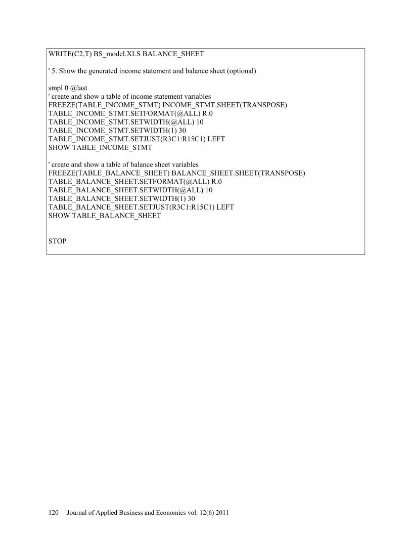
WRITE(C2,T) BS_model.XLS BALANCE_SHEET ' 5. Show the generated income statement and balance sheet (optional) smpl 0 @last ' create and show a table of income statement variables FREEZE(TABLE_INCOME_STMT) INCOME_STMT.SHEET(TRANSPOSE) TABLE_INCOME_STMT.SETFORMAT(@ALL) R.0 TABLE_INCOME_STMT.SETWIDTH(@ALL) 10 TABLE_INCOME_STMT.SETWIDTH(1) 30 TABLE_INCOME_STMT.SETJUST(R3C1:R15C1) LEFT SHOW TABLE_INCOME_STMT ' create and show a table of balance sheet variables FREEZE(TABLE_BALANCE_SHEET) BALANCE_SHEET.SHEET(TRANSPOSE) TABLE_BALANCE_SHEET.SETFORMAT(@ALL) R.0 TABLE_BALANCE_SHEET.SETWIDTH(@ALL) 10 TABLE_BALANCE_SHEET.SETWIDTH(1) 30 TABLE_BALANCE_SHEET.SETJUST(R3C1:R15C1) LEFT SHOW TABLE_BALANCE_SHEET STOP


integrating financial statement modeling and sales ... · integrating financial statement modeling...

Documents