intelligent interpolation for population … · regression-based population estimation models and...

INTELLIGENT INTERPOLATION FOR POPULATION DISTRIBUTION MODELING

by

HWA HWAN KIM

(Under the Direction of XIAOBAI YAO)

ABSTRACT

Dasymetric mapping is an intelligent interpolation method to accurately disaggregate

population distribution with assistance of ancillary data describing the underlying pattern of

geographical phenomena. Many studies have demonstrated that the dasymetric mapping method

can substantially improve accuracy of population estimation by areal interpolation. Despite the

significant performance advantages of the dasymetric method, it has not been widely adopted

amongst broader geography community because of its relative complexity to implement and the

difficulties to acquire high quality ancillary data. This research aims to investigate how to

elaborate the method of dasymetric mapping for population distribution modeling while

minimizing the effort for data acquisition and processing, so as to encourage more users to take

advantage of the dasymetric mapping method for applications involving population distribution

data. This dissertation addresses two questions related to efficient implementation of dasymetric

mapping for population distribution modeling. First is how to improve the performance of

dasymetric mapping method. Second is what kind of public-domain land cover data could be

utilized.

Regression-based population estimation models and three dasymetric mapping methods

are briefly reviewed and tested with the National Land Cover Dataset (NLCD). Although, the

correlation between residential land cover and population density is clearly proved, the relative

performance of the three dasymetric methods (binary, three-class, and limiting variable) is

inconclusive. A hybrid dasymetric method integrating the pycnophylactic interpolation and the

dasymetric mapping significantly outperforms the other methods (areal weighting interpolation,

binary dasymetric mapping, and pycnophylactic interpolation method). Sensitivity analysis

shows that the hybrid method can be further improved with appropriate selection of search radius

size. Geographical weighted regression (GWR) modeling performs very well to estimate

population density weight for each land cover class of the NLCD 2001 data. GWR based multi-

class dasymetric method outperforms other interpolation methods (areal weighting interpolation,

pycnophylactic interpolation, binary dasymetric method, and globally fitted ordinary least

squared (OLS) regression based multi-class dasymetric method). This is attributed to the fact that

spatial heterogeneity is accounted for in the process of determining density parameters for land

cover classes.

INDEX WORDS: Intelligent interpolation, Population, Pycnophylactic interpolation,

Dasymetric mapping, NLCD, Geographically weighted regression


by

HWA HWAN KIM

B.A., Seoul National University, South Korea, 1997

M.A., Seoul National University, South Korea, 2000

B.M., Korean National Open University, South Korea, 2003

A Dissertation Submitted to the Graduate Faculty of The University of Georgia in Partial

Fulfillment of the Requirements for the Degree

DOCTOR OF PHILOSOPHY

ATHENS, GEORGIA

2009

© 2009

HWA HWAN KIM

All Rights Reserved


by

HWA HWAN KIM

Major Professor: Xaiobai Yao

Committee: Thomas Hodler Marguerite Madden Kavita Pandit

Electronic Version Approved: Maureen Grasso Dean of the Graduate School The University of Georgia August 2009

iv

ACKNOWLEDGEMENTS

I would like to express my sincere gratitude to many people. Without their considerable

support, my dissertation research would not have been accomplished. I am deeply indebted to my

major advisor, Dr. Xiaobai Yao for her guidance, encouragement, and support for my doctoral

study and research. Thanks also are due to my committee, Dr. Thomas Hodler, Dr. Marguerite

Madden, and Dr. Kavita Pandit, for their timely assistance and advice. My former advisor, Dr.

Chor-Pang Lo will always remain in my heart. It is so sad to lose such a great mentor. My

appreciations also go to Dr. E. Lynn Usery for his guidance as my first advisor.

I would also like to acknowledge Dr. George Brook, Dr. Steven Holloway, Dr. Marshall

Shepherd, and Dr. Fausto Sarmiento for their thoughtful advice and support. I was more than

happy to have such a nice helping hands of Audrey Hawkins, Kate Blane, Jodie Guy, Emily

Duggar, Loretta Scott, Donna Johnson, and Emily Coffee during my doctoral study in the

Department of Geography. I would also like to thank my fellow graduate students and friends,

Hunter Allen, Sergio Bernades, Bo Xu, Mario Giraldo, Fuyuan Liang, Matt Miller, Minho Kim,

Matt Michelson, Woo Jang, Zaroo Jeong, and Byungyun Yang for their support and friendship in

the last six years.

My sincere thanks also go to the Department of Geography, Graduate School of the

University of Georgia, and the National Science Foundation Dissertation Improvement Grant for

the financial support to my doctoral study and dissertation research. Finally I am grateful to my

parents and my family for their patience, understanding, and support.

v

TABLE OF CONTENTS

Page

ACKNOWLEDGEMENTS........................................................................................................... iv

CHAPTER

1 INTRODUCTION .........................................................................................................1

Research Background................................................................................................1

Research Objectives ..................................................................................................4

Dissertation Organization..........................................................................................5

References .................................................................................................................7

2 POPULATION ESTIMATION USING LAND USE LAND COVER DATA FROM

LANDSAT TM IMAGES .......................................................................................11

Abstract ...................................................................................................................12

Introduction .............................................................................................................13

Study area and data..................................................................................................15

Methodology ...........................................................................................................17

Results .....................................................................................................................21

Conclusion and discussion ......................................................................................25

References ...............................................................................................................27

3 COMPARISON OF THREE DASYMETRIC METHODS FOR POPULATION

DENSITY MAPPING.............................................................................................28

Abstract ...................................................................................................................29

vi

Introduction .............................................................................................................30

Dasymetric mapping approaches.............................................................................32

Study area and data..................................................................................................34

Methodology ...........................................................................................................36

Results .....................................................................................................................41

Discussion and Conclusion .....................................................................................45

References ...............................................................................................................47

4 PYCNOPHYLACTIC INTERPOLATION REVISITED: INTEGRATION WITH

DASYMETRIC MAPPING METHOD..................................................................48

Abstract ...................................................................................................................49

Introduction .............................................................................................................50

Areal interpolation for population estimation .........................................................53

A Hybrid approach for population estimation.........................................................58

Discussion and future research................................................................................73

References ...............................................................................................................75

5 LOCALLY ADAPTIVE INTELLIGENT INTERPOLATION METHOD FOR

POPULATION DISTRIBUTION MODELING USING PRE-CLASSIFIED

LAND COVER DATA ...........................................................................................79

Abstract ...................................................................................................................80

Introduction .............................................................................................................81

Literature review .....................................................................................................85

A GWR-based intelligent interpolation method for population estimation ............96

Conclusions ...........................................................................................................120

vii

References .............................................................................................................121

6 CONCLUSIONS AND FUTURE RESEARCH .......................................................128

Conclusions ...........................................................................................................128

Future Research.....................................................................................................132

References .............................................................................................................135

1

CHAPTER 1

INTRODUCTION

RESEARCH BACKGROUND

Knowledge of the size, characteristics, and spatial distribution of human population is

essential to many applications for governing and planning. Although population data are crucial,

they are typically only available in aggregate forms, such as census blocks or tracts in the United

States, and enumeration districts or wards in the United Kingdom. The spatial aggregation of

census data by street blocks, tracts, and districts is necessary to mask out confidential

information relating to individuals. However, this makes it difficult to map or model the

population distribution accurately, especially when a choropleth mapping approach is used. This

kind of aggregate data cannot sufficiently represent the underlying geographical distributions

fundamental to many planning studies (Bracken 1989; Bracken and Martin 1989; Goodchild et al.

1993; Bracken and Martin 1995; Moon and Farmer 2001). Further, there are well-known scale

and unit specification issues, the modifiable areal unit problem (MAUP), that must be addressed

when statistical or spatial models are applied in the context of planning and decision making

(Fotheringham and Wong 1991; Openshaw and Rao 1995).

In order to address the shortcomings of aggregate census data, researchers have

developed interpolation approaches for transforming areal population counts to raster-based

population density surfaces, which is a process of spatial disaggregation. These interpolation

2

methods can be divided into two groups: simple interpolation and intelligent interpolation

(Langford et al. 1991; Okabe and Sadahiro 1997). Simple interpolation methods include all data

transferring approaches that do not use ancillary data. Many simple interpolation methods have

been detailed in the literature, including area weighted polygon overlay (Lam 1983; Goodchild et

al. 1993), pycnophylactic interpolation (Tobler 1979; Rase 2001), and kernel density functions

(Bracken and Martin 1989, 1995; Martin 1989, 1996; Martin and Bracken 1991). In contrast to

these simple methods, intelligent interpolation methods involve integration with ancillary

information to shed light on the internal variation of population density within each aggregation

unit. Dasymetric mapping method is an example of the intelligent interpolation method, which

has been increasingly popular due to the emergence and growing popularity of Geographic

Information System (GIS) and Remote Sensing (RS) technologies. Various data sources have

been used as ancillary information. Examples include nighttime satellite imagery using the

visible near-infrared(IR) band (Sutton 1997; Dobson et al. 2000; Sutton et al. 2001), housing

distribution data (Moon and Farmer 2001), land property parcel data (Luo 2005), vector street

networks (Mrozinski and Cromley 1999; Reibel and Bufalino 2005), vector land cover data

(Eicher and Brewer 2001; Mennis 2003), and raster land cover data derived from classified

satellite imagery (Langford and Unwin 1994; Yuan et al. 1997; Holt et al. 2004; Sleeter 2004;

Reibel and Agrawal 2007). Among those, land use and land cover dataset is the most commonly

used, given that it is highly correlated with population density (Wright 1936; Flowerdew and

Green 1989; Langford et al. 1991; Langford and Unwin 1994; Langford 2006). Many studies

have demonstrated that the dasymetric mapping method can substantially improve the accuracy

of population density estimation (Fisher and Langford 1995; Cockings et al. 1997; Mrozinski

and Cromley 1999; Langford 2006; Reibel and Agrawal 2007).

3

Despite the significant performance advantages of the dasymetric mapping method, there

has been little evidence to suggest widespread adoption amongst the broader GIS community

(Langford 2007). Langford (2007) stated that intelligent methods, such as dasymetric mapping

method, were not widely adopted because of two reasons. Firstly, an implementation of

intelligent interpolation is much more complicated than simple interpolation. Furthermore, most

intelligent interpolation methods require an additional process to prepare ancillary information.

Therefore, it is no wonder that many users still prefer the traditional simple interpolation method

despite the superior performances by intelligent interpolation methods reported in many studies.

There are positive and negative factors that encourage or discourage users from adopting

dasymetric mapping method. To encourage a broader geography community to employ

dasymetric mapping methods for its advantages in population distribution estimation accuracy,

efforts should be made to overcome the problems of excessive processing time and

implementation difficulty while ensuring its performance. Regarding the acquisition of high

accuracy ancillary information, there are several types of public-domain high quality datasets

available in the United States such as the Multi-Resolution Land Characteristic Consortium

(MRLC) National Land Cover Dataset (NLCD).

4

RESEARCH OBJECTIVES

The overall aim of this research is to investigate how to elaborate the method of

dasymetric mapping for population distribution modeling while minimizing effort for ancillary

data acquisition and processing, so as to encourage more users to exploit advantages of

dasymetric mapping method for their applications involving population distribution data. This

dissertation addresses two questions related to efficient implementation of dasymetric mapping

method for population distribution modeling. The first is how to improve the performance of

dasymetric mapping method. Second is what kind of public-domain land use land cover data are

available, and how those could be utilized. Specifically, the objectives of this dissertation are:

1. To evaluate the performance of different population estimation models based on

multiple regression analysis,

2. To present and examine correlations between population density and land use land cover

classes of the public-domain National Land Cover Dataset (NLCD),

3. To investigate and compare performances of different dasymetric mapping methods

using the NLCD data,

4. To examine advantages of pycnophylactic interpolation for population distribution

modeling, and to investigate merits of integrating pycnophylactic interpolation with

dasymetric mapping method,

5. To investigate the spatial heterogeneity of the relationship between land cover types and

population densities, and to develop an intelligent interpolation method to account for

the spatial heterogeneity in population distribution modeling.

5

DISSERTATION ORGANIZATION

The dissertation consists of four interrelated research papers. The first paper in Chapter 2

briefly reviews population estimation research using remotely sensed data. It evaluates the

performance of four statistical estimation models using the NLCD 1992 and the U.S. Census

1990 population count data. The results of the chapter show how the distribution of land use land

cover is closely related to population distribution. The ‘focused’ and ‘simple’ models that use

only residential land use class give the best estimation in terms of the absolute mean relative

error measure. Spatial distribution of relative errors shows a clear tendency of underestimation in

high-density populated area and overestimation in the low-density area. The second paper in

Chapter 3 compares performances of different dasymetric methods. Three schemes (binary,

three-class, and limiting variable) of dasymetric mapping method are tested on Athens, GA using

the NLCD 1992 and the 1990 U.S. Census population count data. All three dasymetric methods

perform significantly better than the conventional areal weighting interpolation method. The

limiting variable method seems to perform best according to the root mean squared error

(RMSE) measure. However its superiority is inconclusive. The third paper in Chapter 4 presents

the development a hybrid intelligent interpolation method integrating the pycnophylactic

interpolation and the dasymetric mapping method. Each of the methods has its own strength but

also suffers obvious shortcomings. The hybrid approach takes advantage of the strengths of both

methods while overcoming the drawbacks of them.

The performance of the hybrid method is evaluated by comparing its estimation

accuracy with those of other popular methods including areal weighting interpolation, binary

dasymetric mapping, and pycnophylactic interpolation method. The comparison results prove

that the hybrid method significantly outperforms the other methods. A sensitivity analysis

6

examining the effect of search radius size shows that the hybrid method can be further improved

with appropriate choice of search radius. The fourth paper in Chapter 5 examines the benefits of

the geographical weighted regression (GWR) model for dasymetric density parameter estimation

using the pre-classified NLCD 2001 land cover dataset. The performance of the GWR based

multi-class dasymetric mapping method is examined by a comparative accuracy assessment with

four other areal interpolation methods including areal weighting interpolation, pycnophylactic

interpolation, binary dasymetric method, and globally fitted ordinary least squared (OLS) based

multi-class dasymetric method. GWR based multi-class dasymetric method outperforms the

other methods. It is attributed to the fact that spatial heterogeneity is accounted for in the process

of determining density parameters for land cover classes.

7

REFERENCES

Bracken, I. 1989. The generation of socioeconomic surfaces for public policymaking.

Environment & Planning B: Planning and Design 16:307-325.

Bracken, I., and D. Martin. 1989. The generation of spatial population distributions from census

centroid data. Environment & Planning A 21:537-543.

———. 1995. Linkage of the 1981 and 1991 UK Censuses using surface modelling concepts.

Environment & Planning A 27:379-390.

Cockings, S., P. F. Fisher, and M. Langford. 1997. Parameterization and Visualization of the

Errors in Areal Interpolation. Geographical Analysis 29 (4):314-328.

Dobson, J. E., E. A. Bright, R. Coleman, R. G. Durfee, and B. A. Worley. 2000. LandScan: A

global population database for estimating population at risk. Photogrammetric

Engineering & Remote Sensing 66 (7):849-857.

Eicher, C., and C. Brewer. 2001. Dasymetric mapping and areal interpolation: implementation

and evaluation. Cartography and Geographic Information Science 28:125-138.

Fisher, P. F., and M. Langford. 1995. Modelling the errors in areal interpolation between zonal

systems by Monte Carlo Simulation. Environment & Planning A 27:211-224.

Flowerdew, R., and M. Green. 1989. Statistical methods for inference between incompatible

zonal systems. In The Accuracy of Spatial Databases, eds. M. F. Goodchild and S. Gopal,

239-247. London: Taylor and Francis.

Fotheringham, A. S., and D. W. S. Wong. 1991. The modifiable areal unit proble in multivariate

statistical analysis. Environment & Planning A 23:1025-1044.

Goodchild, M. F., L. Anselin, and U. Deichmann. 1993. A framework for the areal interpolation

of socioeconomic data. Environment and Planning A 25 (3):383-397.

8

Holt, J. B., C. P. Lo, and T. W. Hodler. 2004. Dasymetric estimation of population density and

areal interpolation of census data. Cartography and Geographic Information Science 31

(2):103-121.

Lam, N. S. 1983. Spatial interpolation methods: a review. The American Cartographer 10

(2):129-149.

Langford, M. 2006. Obtaining population estimates in non-census reporting zones: An evaluation

of the 3-class dasymetric method. Computers, Environment and Urban Systems 30

(2):161-180.

———. 2007. Rapid facilitation of dasymetric-based population interpolation by means of raster

pixel maps. Computers, Environment and Urban Systems 31 (1):19-32.

Langford, M., D. J. Maguire, and D. J. Unwin. 1991. The areal interpolation problem: estimating

population using remote sensing within a GIS framework. In Handling Geographical

Information: Methodology and Potential Applications, eds. I. Masser and M. Blackmore,

55-77. London: Longman.

Langford, M., and D. J. Unwin. 1994. Generating and mapping population density surfaces

within a geographical information system. The Cartographic Journal 31 (June):21-25.

Luo, J. 2005. Analyzing urban spatial structure with GIS population surface model. Paper read at

UCGIS summer assembly, at Jackson hall, Wyoming.

Mennis, J. 2003. Generating Surface Models of Population Using Dasymetric Mapping. The

Professional Geographer 55 (1):31-42.

Moon, Z. K., and F. L. Farmer. 2001. Population Density Surface: A New Approch to an Old

Problem. Society and Natural Resources 14:39-49.

9

Mrozinski, R. D., and R. G. Cromley. 1999. Singly - and Doubly - Constrained Methods of Areal

Interpolation for Vector-based GIS. Transactions in GIS 3 (3):285-301.

Okabe, A., and Y. Sadahiro. 1997. Variation in count data transferred from a set of irregular

zones to a set of regular zones through the point-in-polygon method. International

Journal of Geographical Information Science 11:93-106.

Openshaw, S., and L. Rao. 1995. Algorithms for reengineering 1991 Census geography.


Rase, W. 2001. Volume-preserving interpolation of a smooth surface from polygon-related data.

Journal of Geographical Systems 3 (2):199.

Reibel, M., and A. Agrawal. 2007. Areal Interpolation of Population Counts Using Pre-classified

Land Cover Data. Population Research and Policy Review 26:619-633.

Reibel, M., and M. E. Bufalino. 2005. Street-weighted interpolation techniques for demographic

count estimation in incompatible zone systems. Environment and Planning A 37:127-139.

Sleeter, R. 2004. Dasymetric mapping techniques for the San Francisco bay region, California.

Paper read at Urban and Regional Information Systems Association Annual Conference,

November 7–10, 2004., at Reno, NV.

Sutton, P. 1997. Modeling population density with night-time satellite imagery and GIS.

Computers, Environment and Urban Systems 21 (3-4):227-244.

Sutton, P., D. Roberts, C. Elvidge, and K. Baugh. 2001. Census from Heaven: an estimate of the

global human population using night-time satellite imagery. International Journal of

Remote Sensing 22 (16):3061-3076.

Tobler, W. 1979. Smooth pycnophylactic interpolation for geographic regions. Journal of the

American Statistical Association 74 (367):519-536.

10

Wright, J. K. 1936. A method of mapping densities of population with Cape Cod as an example.

Geographical Review 26:103-110.

Yuan, Y., R. M. Smith, and W. F. Limp. 1997. Remodeling census population with spatial

information from LandSat TM imagery. Computers, Environment and Urban Systems 21

(3-4):245-258.

11

CHAPTER 2

POPULATION ESTIMATION USING LAND USE LAND COVER DATA FROM

LANDSAT TM IMAGES - IMPLEMENTATION AND LIMITATIONS 1

1 Kim, H, 2006. The Geographical Journal of Korea. 40(4):489-496. Reprinted here with permission of publisher.

12

ABSTRACT

Accurate population estimation is one of the most essential techniques to supplement

decennial census data. The expanded and timely availability of remotely sensed data provides a

practical way to estimate between-census population for a small area by incorporating land use

land cover information extracted from satellite images into estimation process. The accuracy of

population estimation with land use land cover data is determined by several factors. Besides the

accuracy of image classification, the explicit statistical relationship between land use land cover

information and actual population count has a critical importance for effective estimation. The

statistical relationship is modeled by a regression analysis where pixel counts of land use land

cover are used as independent variables and population counts as the dependent variable,

respectively. This research tests several regression models to explore the statistical relationship

between land use characteristic and population counts. The performance of each model is

evaluated in two ways. First, the estimated total population of the study area is compared to the

actual census population. The allometric growth model based on the strong relationship between

the logarithmic value of population and the number of high-density residential pixels gives the

closest estimate in terms of total population count. Second, the regression coefficients calculated

by the regression analysis with sampled U.S. Census Bureau block groups are utilized to estimate

population counts in the all census block groups. The ‘focused’ model and ‘simple’ model that

use only residential pixels give the best estimation in terms of the absolute mean relative error.

Spatial distribution of relative errors shows a clear tendency of underestimation in high-density

populated area and overestimation in the low-density area. Keywords: population estimation,

census population, land use land cover, remote sensing, Landsat TM imagery, regression

analysis, allometric growth model

13

INTRODUCTION

Accurate and timely population data are essential to most regional policy issue and

related geographic research using socio-economic variables. Most population censuses are very

expensive, and normally conducted only every decade even in the developed countries (Lo 1995;

Qiu et al. 2003). For these reasons, demographic models have been employed in order to predict

intercensal population based on previous census figures combined with a variety of other data,

such as local economic indicators, counts obtained from consumer marketing databases, postal

service delivery statistics, etc. These methods may provide reasonable estimations, but the

implementation of these models is often complex and expensive due to the requirement for

collecting multiple inputs and the need of significant manpower for analysis.

Remotely sensed images provide alternative opportunities for estimating population in

urban and suburban areas. Large scale aerial photographs have long been used to count the

number of dwelling units observed from the sky and to estimate total population based on

average household size for each dwelling type (Lo 1986a). This method provides very accurate

counts of dwelling units, but it requires a large number of aerial photographs and is very time-

consuming, so it is only suited for use in small areas. With the increased availability of high

resolution satellite images such as SPOT 20-meter spatial resolution multi-spectral scanner data

and LANDSAT Thematic Mapper (TM) 30-meter resolution data, they can be imported to a

computer and analyzed by a raster-based geographic information system (GIS).

14

Lo (1986b) distinguished four different approaches to population estimation from

remotely sensed imagery as following:

a) Counts of dwelling units;

b) Measurement of areas of urbanization;

c) Measurement of areas of different land use;

d) Automated digital image analysis

Among these categories, the third approach, applicable at small to medium scales with

medium resolution imagery, has been applied in various ways to estimated population and related

demographic characteristics. Increases in areas of urbanization have been monitored in many

studies using techniques for change detection and land use classification (Harvey 2002).

Langford et al. (1991) used a classification approach to estimate the populations of 49 census

wards in northern Leicestershire in United Kingdom. The explanatory variables were the

numbers of pixels in each of five land use categories (dense residential, ordinary residential,

industrial / commercial, logically with no population, agricultural), obtained by supervised

classification of a Landsat TM image. Lo (1995) used a mixture of both types of predictor (mean

reflectance and counts of pixels in classes) to estimate the population and dwelling unit numbers

in 44 tertiary planning units of Kowloon, Hong Kong, using multi-spectral SPOT imagery.

The purpose of this paper is to implement the population estimation in Athens-Clarke

County, Georgia. according to the methods suggested by Langford et al. (1991) and Lo (1995)

using land use land cover data, and visually explore the spatial variations of estimation accuracy

in the context of regional characteristics. Some limitations of implementing these methods and

considerations are commented upon.

15

STUDY AREA AND DATA

Study Area

Athens-Clarke County, a university town in north east of the state of Georgia, is used as

the study area (Figure 2-1). The County has total population of 87,594 according to the U. S.

Census Bureau’s 1990 census.

Figure 2-1. Study area; Athens-Clarke County, Georgia in Census block groups

16

Data

The two datasets used for the case study are as follows:

U.S. Census Bureau, TIGER 98 Block Groups (UTM) joined with 1990 census data

National Land Cover Dataset (NLCD) 1992 from Georgia GIS Data Clearinghouse

This land cover dataset was produced as part of a cooperative project between the U.S.

Geological Survey (USGS) and the U.S. Environmental Protection Agency (EPA) to produce a

consistent, land cover data layer for the conterminous U.S. based on 30-meter Landsat Thematic

Mapper (TM) images. The base dataset for this project was leaf-on Landsat TM data, nominal-

1992 acquisitions (Figure 2-2). The 23-Class National Land Cover Data Key is used for

supervised classification (Vogelmann et al. 1998).

Figure 2-2. The National Land Cover Dataset (NLCD) 1992

17

METHODOLOGY

Data preparation

For analytical purposes, the 23-class National Land Cover Dataset was reclassified into a

simplified land cover dataset with only 5 land cover classes as following (Figure 2-3):

a) Low Intensity Residential - Low_res

b) High Intensity Residential - High_res

c) Commercial/Industrial/Transportation - Comm

d) Areas that logically have no population (Water, Barren lands, Forested Uplands,

Wetlands, and Urban/Recreational Grasses) - Nobody

e) Agricultural Lands (Pasture/Hay, Row Crops) - Agric

Figure 2-3. Reclassified land cover of study area

18

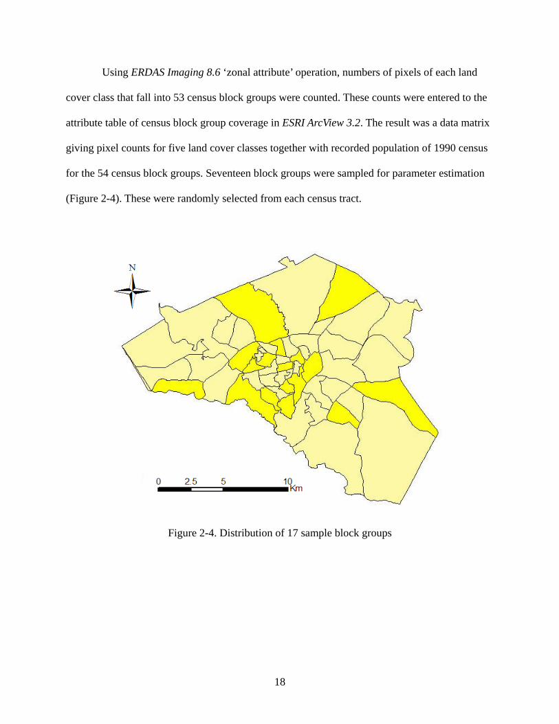
Using ERDAS Imaging 8.6 ‘zonal attribute’ operation, numbers of pixels of each land

cover class that fall into 53 census block groups were counted. These counts were entered to the

attribute table of census block group coverage in ESRI ArcView 3.2. The result was a data matrix

giving pixel counts for five land cover classes together with recorded population of 1990 census

for the 54 census block groups. Seventeen block groups were sampled for parameter estimation

(Figure 2-4). These were randomly selected from each census tract.

Figure 2-4. Distribution of 17 sample block groups

19

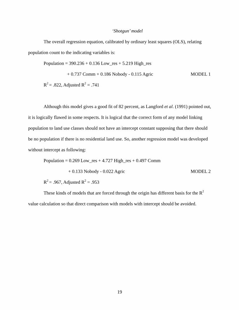
‘Shotgun’ model

The overall regression equation, calibrated by ordinary least squares (OLS), relating

population count to the indicating variables is:

Population = 390.236 + 0.136 Low_res + 5.219 High_res

+ 0.737 Comm + 0.186 Nobody - 0.115 Agric MODEL 1

R2 = .822, Adjusted R2 = .741

Although this model gives a good fit of 82 percent, as Langford et al. (1991) pointed out,

it is logically flawed in some respects. It is logical that the correct form of any model linking

population to land use classes should not have an intercept constant supposing that there should

be no population if there is no residential land use. So, another regression model was developed

without intercept as following:

Population = 0.269 Low_res + 4.727 High_res + 0.497 Comm

+ 0.133 Nobody - 0.022 Agric MODEL 2

R2 = .967, Adjusted R2 = .953

These kinds of models that are forced through the origin has different basis for the R2

value calculation so that direct comparison with models with intercept should be avoided.

20

‘Focused’ model

Any statistical model linking pixel counts of land cover to population should be simple,

linear, additive, and without any intercept constant. In this model, the individual coefficients

have a direct interpretation as the average density of people in each pixel of specified type. With

only residential (high intensity and low intensity) land use pixel counts, following model were

developed:

Population = 0.915 Low_res + 3.668 High_res MODEL 3

R2 = .917, Adjusted R2 = .906

‘Simple’ model

As the simplest of all, pixel counts of high intensity residential and low intensity

residential were summed up and regressed against population in simple linear model:

Population = 1.370 Residential MODEL 4

R2 = .865, Adjusted R2 = .857

Allometric growth method

Allometric growth model is based on the strong relationship between the common

logarithmic value of population and the absolute number of high-density residential pixels (Lo

1995). The equation took the following allometric growth form:

Log10population = 2.623 + 0.281 log10 High_res MODEL 5

R2 = .632, Adjusted R2 = .612

21

RESULTS

According to the coefficients extracted from the 17 sample census block groups by five

different models, five population value matrices were calculated for all 54 block groups of the

study area. Relative errors of population estimation by each model for the whole study area were

summarized in Table 2-1. In each result, relative error after exclusion of extreme outliers that are

over or underestimated over 100% is additionally calculated.

Table 2-1. Relative errors respective to each model

MODEL 1 MODEL 2 MODEL 3 MODEL 4 MODEL 5

Estimated population 106,228 96,370 79,638 77,297 86,303

Relative error (%) 21.27% 10.02% -9.08% -11.76% -1.47%

Relative error after exclusion of extreme outliers

8.89% 9 excluded

1.49% 6 excluded

-10.71% 2 excluded

-12.55% 1 excluded

-8.09% 5 excluded

Absolute mean relative error (%) 85.55% 49.08% 34.68% 34.75% 55.15%

Note: 1990 Census population of Athens-Clarke county is 87,594

‘Shotgun’ model

The first method which employed regression model using 5 explanatory variables of

land cover classes overestimated overall population by 21.27% and 10.02% (the model without

intercept) respectively. These relative errors improved to 8.89%, 1.49% after excluding extreme

outliers. But, those outliers make up considerable proportion of total census block groups so that

this result is hard to be evaluated as a good estimation.

22

‘Focused’ and ‘Simple’ model

The second and third method which employed regression models with only residential

land cover classes underestimated overall population by -9.08% and -11.76% respectively. These

relative errors deteriorated to -10.71% and -12.55% after excluding extreme outliers. But, few

outliers and relatively small amount of absolute mean relative errors showed that it can be

evaluated as meaningful in micro level.

Allometric growth model

The fourth method that employed the allometric growth relationship estimated overall

population with a relative error of -1.47%. It is the most accurate estimation out of all models.

But, after exclusion of five extreme outliers, relative error deteriorated to -8.09%. It can be said

that the allometric growth approach was the most accurate method to estimate population for the

whole area. But, for population at the census block group level, Model 3 and 4 which use only

residential land cover can be preferred.

23

Relative error distribution

In addition to the descriptive evaluation about the results of the five estimation models,

relative error for each census block group can be displayed and visually interpreted so the spatial

implication of those methods can be explored.

Figures 2-5 and 2-6 show the spatial distribution of relative errors estimated by Model 1

and 2 which employed all land cover categories. In the relation with population density map of

study area (Figure 2-10), both figures show that overestimated block groups tends to be found in

low population density area, and by contrast, underestimated block groups mainly can be found

in high population density area. In Model 3 and 4, this tendency is reduced, but still city center

area tends to be underestimated by these models (Figure 2-7 and 2-8). In case of Model 5 which

employed logarithmic relationship between population and high intensity residential land cover,

this tendency hardly can be found (Figure 2-9).

Figure 2-5. Error distribution (Shotgun) Figure 2-6. Error distribution

(Shotgun without intercept)

24

Figure 2-7. Error distribution (Focused) Figure 2-8. Error distribution (Simple)

Figure 2-9. Error distribution

(Allometric growth)

Figure 2-10. Actual population density

distribution

25

CONCLUSIONS AND DISCUSSION

In this paper, a number of population estimation models are implemented and evaluated

with the NLCD 1992 that is produced by classification of Landsat TM satellite images. In overall

population estimation, the allometric growth model was found to make the best estimation. On

the other hand, in census block group level, those methods which employ regression model

between population and counts of pixels that fall into residential land cover classes (high

intensity residential and low intensity residential) showed the best results. These methods

however did not increase accuracy and generally it can be said that the accuracy of estimation at

the census block group level was much lower. This can be on account of various causes. First,

Athens-Clarke County is a university town encompassing complicated housing patterns like

student dormitory and family housing complexes for married students, as well as ordinary style

single-family housing units. Those high intensity residential land uses are not common in other

parts of the city, which may create a difficulty in accurate population estimation using land cover

data from satellite images. Second, in spite of the small size of the study area, Athens-Clarke

County encompasses 54 census block groups which have various population density levels from

29 persons to 10,865 persons per kilometer square. So, it is naturally hard to make a common

population estimation model.

26

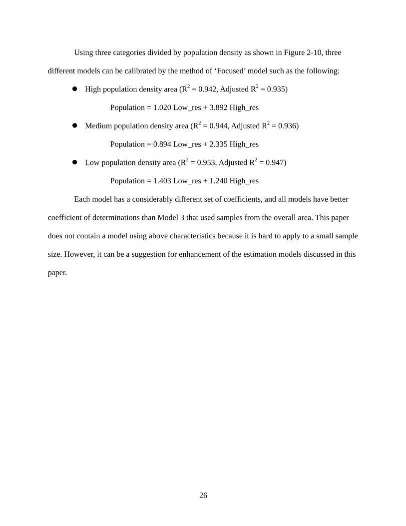
Using three categories divided by population density as shown in Figure 2-10, three

different models can be calibrated by the method of ‘Focused’ model such as the following:

High population density area (R2 = 0.942, Adjusted R2 = 0.935)

Population = 1.020 Low_res + 3.892 High_res

Medium population density area (R2 = 0.944, Adjusted R2 = 0.936)


Low population density area (R2 = 0.953, Adjusted R2 = 0.947)


Each model has a considerably different set of coefficients, and all models have better

coefficient of determinations than Model 3 that used samples from the overall area. This paper

does not contain a model using above characteristics because it is hard to apply to a small sample

size. However, it can be a suggestion for enhancement of the estimation models discussed in this

paper.

27

REFERENCES

Harvey, J. T. 2002. Estimating census district populations from satellite imagery: some

approaches and limitations. International Journal of Remote Sensing 23 (10):2071-2095.





Lo, C. 1986a. Accuracy of population estimation from medium-scale aerial photography.

Photogrammetric Engineering and Remote Sensing 52:1859-1869.

———. 1986b. Applied Remote Sensing: Harlow: Longman.

———. 1995. Automated population and dwelling unit estimation from high-resolution satellite

images: a GIS approach. International Journal of Remote Sensing 16:17-34.

Qiu, F., K. L. Woller, and R. Briggs. 2003. Modeling Urban Population Growth from Remotely

Sensed Imagery and TIGER GIS Road Data. Photogrammetric Engineering and Remote

Sensing 69 (5):1031-1042.

Vogelmann, J. E., T. L. Sohl, P. V. Campbell, and D. M. Shaw. 1998. Regional Land Cover

Characterization Using Landsat Thematic Mapper Data And Ancillary Data Sources.

Environmental Monitoring and Assessment 51:415-428.

28

CHAPTER 3

COMPARISON OF THREE DASYMETRIC METHODS FOR POPULATION DENSITY

MAPPING 2

2 Kim, H, 2007. The Geographical Journal of Korea. 41(4):411-419. Reprinted here with permission of publisher.

29

ABSTRACT

This paper explores a raster-based population estimation using dasymetric mapping

techniques that incorporate land use land cover data as a means to redistribute the original census

population value into a surface grid. The three methods reviewed by Eicher and Brewer (2001)

are tested in Athens-Clarke County, Georgia. Using the three (binary, three-class, and limiting

variable) methods, and the conventional choropleth method, I estimate total populations of 54

U.S. Census Block Groups to quantify how well those models reflect real population distribution.

Bivariate regression analysis is used to look at how estimation errors vary across cases. All three

dasymetric methods perform significantly better than the conventional choropleth method. In

terms of RMS error and mean coefficient of variation, the limiting variable method performs

slightly better than others. The correlation coefficients for dasymetric methods are high, ranging

from 0.916 to 0.94. Also, a simple form of error distribution maps is used to visualize how

estimation errors are spatially distributed for each estimation model. Keywords: Dasymetric

mapping, Choropleth mapping, Population density, Land use land cover

30

INTRODUCTION

Demographic data are commonly displayed cartographically using the choropleth

mapping technique. For example, choropleth maps are used to display U.S. Census data, a

geographic standard for demographics, and are used as a medium by virtually all geographers

and many non-geographers (Slocum and Egbert 1993). The choropleth map spatially aggregates

data into geographic areas or areal units (e.g., county, census tract, block group, etc.). Because

the value in the enumeration unit is assumed to be uniform throughout the areal unit, continuous

geographic phenomena cannot be properly displayed (Goodchild 1992). Dorling (1993) noted

that choropleth maps of population by areal unit system give the notion that population is

distributed homogeneously throughout each areal unit, even when proportions of the region are,

in reality, uninhabited. This discrepancy is greatest in areas with mixed urban, agricultural, and

uninhabitable land uses.

Dasymetric mapping is a potential solution for the dilemma of portraying population

data that have been aggregated into areal units. The dasymetric mapping depicts quantitative

areal data using boundaries that divide the mapped area into zones of relative homogeneity with

the purpose of portraying the underlying statistical surface (Eicher and Brewer 2001). This type

of mapping has been described as an intelligent approach to choropleth mapping in an attempt to

improve areal homogeneity. Thus, new zones are created that directly relate to the function of the

map, which is to show spatial variations in population density. Land cover data can indicate

residential areas for the delineation of new homogeneous zones. The census populations can be

redistributed to the new zones, resulting in a more accurate portrayal of where people live within

an enumeration boundary.

31

Dasymetric mapping differs from choropleth mapping in that the boundaries of

cartographic representation are not arbitrary but reflect the spatial distribution of the variable

being mapped. Eicher and Brewer (2001) reviewed and evaluated a number of dasymetric

mapping techniques to allot population to dasymetric zones: binary, three-class, and limiting

variable.

This study explores a surface-based representation of population, using a dasymetric

mapping technique that incorporates land cover data as a means to redistribute the original

census population value into a surface grid. Specifically, the three methods reviewed by Eicher

and Brewer (2001) are tested for more accurate representation of where people live in Athens-

Clarke County, Georgia. The results are evaluated by comparison between original zonal

population of smaller spatial units (census block group) and estimated population using the three

methods built from larger spatial units (census tract). I hypothesize that the census tracts

populations on the dasymetric map will show a statistically superior match to the census block

group populations over those on the choropleth map.

32

DASYMETRIC MAPPING APPROACHES

An essential step in dasymetric mapping is the creation of zones within the areal unit that

correspond to the variable being mapped. To create intra-unit zones of relative homogeneity

among population, ancillary data must be used to interpret relative levels of habitation. Past

approaches have focused on using ownership records, topography, and land cover classifications

to identify and mask uninhabited areas. Holloway et al. (1999) used multiple datasets to detect

and remove uninhabited lands from the area of analysis. Four types of area were ruled out,

including census blocks with zero population, all lands owned by local, State, or Federal

government, all corporate timberlands, and all water or wetlands, as well as all open and wooded

areas with elevation data that have a slope of less than 15% (Holloway et al. 1999). To

redistribute the census population to the ancillary feature classes, Eicher and Brewer (2001)

compares three methods: binary, three-class, and limiting variable. In the binary method, the land

use land cover classes are split into two groups: habitable and uninhabitable. The habitable group

may include urban and agricultural categories, and the uninhabitable group consists of the water

and forested categories. One hundred percent of the population is assigned to the habitable group

and zero percent to the uninhabitable group.

In the three-class method, land use land cover classes are grouped into three classes in

addition to uninhabitable group, and then a predetermined percentage is assigned to each class.

While improving the accuracy of population distribution, this method suffers from a critical

weakness. The subjectivity and accuracy of this percentage assignment (e.g., 70% of the

population to residential pixels, 20% to commercial, and 10% to agricultural) can be argued

because of the absence of empirical evidence.

33

Limiting variable method is an approach developed by Wright (1936). In this approach,

the population is first assigned so that the density of the habitable categories is identical. At this

step, uninhabitable class is “limited” to zero density. Next, we set thresholds of maximum

density for particular land uses and apply these throughout the study area. For example,

commercial / industrial areas are limited to 50 people per square kilometer and agricultural areas

are assigned a lower threshold of 15 people per square kilometer for the total population variable

to be mapped. The final step in the mapping process is the use of these threshold values to make

adjustments to the data distribution within each source zone. Population density of sub-regions

other than that of limiting variable is calculated by following:

m

mmn a

aDDD

−−

=1

Where a region has been divided into two areas n and m, D is the overall density of the

region, Dm is the threshold density set to sub-region m, am is the fractional area of region n

(relative to the entire region), and Dn is the density of region n. To decide the upper limits on the

densities of the limiting variable, Eicher and Brewer (2001) used source zones that were

classified entirely as one class to set the threshold value.

34

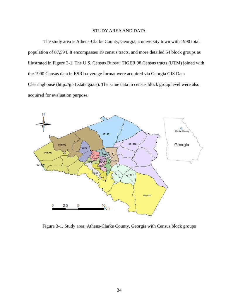
STUDY AREA AND DATA

The study area is Athens-Clarke County, Georgia, a university town with 1990 total

population of 87,594. It encompasses 19 census tracts, and more detailed 54 block groups as

illustrated in Figure 3-1. The U.S. Census Bureau TIGER 98 Census tracts (UTM) joined with

the 1990 Census data in ESRI coverage format were acquired via Georgia GIS Data

Clearinghouse (http://gis1.state.ga.us). The same data in census block group level were also

acquired for evaluation purpose.

Figure 3-1. Study area; Athens-Clarke County, Georgia with Census block groups

35

A necessary element for dasymetric mapping is an ancillary dataset. This information is

used to assist interpolation of data from the original source zones to new target zones (e.g.

regular grid). The National Land Cover Dataset (NLCD) 1992 of the study area (Figure 3-2) was

also acquired for this purpose via Georgia GIS Data Clearinghouse.

The land cover dataset was produced as part of a cooperative project between the U.S.

Geological Survey (USGS) and the U.S. Environmental Protection Agency (USEPA) to produce

a consistent, land cover data layer for the conterminous U.S. based on 30-meter Landsat

Thematic Mapper (TM) data. The base dataset for this project was leaf-on Landsat TM data,

nominal-1992 acquisitions. The total 23-Class National Land Cover Data Keys were used for

supervised classification (Vogelmann et al. 1998).

Figure 3-2. The National Land Cover Dataset (NLCD) 1992

36

METHODOLOGY

My approach combines the methodologies of Mennis (2003) and Holloway et al. (1999)

by choosing four land cover classes, using a three-tier urbanization classification and adding an

excluded class representing zero population. The 23 class NLCD is recoded into four classes;

high-intensity residential, low-intensity residential, commercial / Industrial, agricultural, and

uninhabitable as shown in Figure 3-3. The uninhabitable class incorporates lands that have some

recreational, open-space, and water. The advantage of incorporating an uninhabitable class is to

more accurately display population density by weeding out large areas of the areal interpolation,

allowing the visual depiction of population to be strictly within those areas that are actually

populated.

Figure 3-3. Reclassified land cover of study area

37

After the recoding process, the new zones that have enhanced homogeneity are prepared

in a raster format. Using ERDAS Imagine 8.6 zonal attribute operation, numbers of pixels of each

category that fall into 19 census tracts are counted. These counts are entered to the attribute table

of census tract coverage in ESRI ArcView 3.2. The result is a data matrix giving pixel counts for

five land cover types together with recorded population of 1990 census for the 19 census tract as

shown in Table 3-1. Based on the land cover information for each census tract, population

densities for the whole set of land cover categories are calculated using three dasymetric methods

are developed in addition to simple choropleth method. Finally, the density values are assigned to

census block groups that are included in each tract to estimate block group populations through

reverse calculation.

38

Table 3-1. Census tract attribute table joined with land cover pixel counts

ID AREA(m2) POP TOTAL LOW RES

HIGH RES COMM AGRIC Uninhabitable

9 866411.0 921 978 140 16 640 19 163

7 2651041.4 1864 2940 917 362 1077 37 547

6 6807517.8 6119 7547 2647 843 750 213 3094

13 2984265.2 3225 3284 435 530 929 540 850

14 398242.0 4326 461 152 249 8 1 51

11 1601578.5 3563 1780 617 519 431 8 205

8 3077218.6 3513 3439 1618 756 502 21 542

4 7709715.2 3349 8587 3112 508 752 125 4090

12 2359420.1 3646 2665 1068 723 369 10 495

15 1878919.6 3707 2073 1036 457 230 1 349

17 4621401.4 4941 5251 1993 558 389 95 2216

16 3555512.0 2550 3825 1699 448 166 13 1499

2 38338464.8 7104 42541 4848 372 1545 5528 30119

5 38715338.8 6956 43277 5154 1046 1855 3500 31648

1 40324537.6 5554 44738 3425 257 1023 6813 32939

3 62863954.7 6756 70053 4690 677 2532 20601 41496

19 17131226.6 11685 19301 6927 1590 840 806 9138

18 77875384.0 7788 87105 5760 264 953 16913 62948

10 486084.3 27 669 9 0 1 38 135

39

Choropleth method

The choropleth method divides tract population with the number of all pixels that fall

into the tract boundary to get a single density value regardless of difference in land cover.

i

ii A

PD = Where, Pi is population of tract i and Ai is area of tract i.

Binary method

In the binary method, the land use land cover categories are split into two groups:

residential and non-residential. All categories other than high density residential and low density

residential are included in the non-residential group. Then, a hundred percent of the population is

assigned to the residential and zero percent to the non-residential group.

ri

iri A

PD = Where, Dri is population density for residential area only and Ari is

residential sub-area of tract i.

Three-class method

In the three-class method, land use land cover categories are grouped into three classes

other than uninhabitable class, and then a predetermined percentage is assigned to each class. In

this study, 70% of the population is assigned to residential pixels, 20% to commercial, 10% to

agricultural, and 0% to uninhabitable class.

ki

ikik A

PfD ×= Where, Dik is population density for class k of tract i, fk is the fraction

of population assigned to the class k, and Aki is area of class k in tract i.

40

Limiting variable method

Limiting variable method assigns population to each class so that the density of the

habitable categories is identical. Next, threshold density values for particular land uses are set

and applied. In this study, commercial / industrial areas are limited to 50 people per km2 and

agricultural areas are assigned a lower threshold of 30 people per km2 for the total population

variable to be mapped. The final step in the mapping process is the use of these threshold values

to make adjustments to the data distribution within each source zone. Since the density values for

the other two habitable classes are set, adjustment by limiting variables is applied only to

residential class as follow:

ri

kkkii

ri A

DAPD

∑ ×−=

)( Where, Dk is predetermined density threshold for class k.

Using the above four methods, I estimate total populations of 54 census block groups to

quantify how well those models reflect real population distribution. Population density values

acquired by the four methods are assigned each census block group by which census tract the

block group is included. Total population of each block group is also calculated by equations

above.

41

A variety of ways of measuring error have been used in areal interpolation research. I

followed Fisher and Langford (1995) in their use of root mean squared error (RMSE) and a

coefficient of variation (C.V.) to describe errors in dasymetric zones because RMSE can be

applied to count data (e.g., total number of people) and is easily interpreted as a value with the

same units as the mapped variable. The coefficient of variation for each block group is calculated

by dividing the RMSE by the correct block group population. To further test a positive

association between the block group population totals and the dasymetric mapping distributions,

I conducted a correlation analysis. The correlation coefficient, denoted by r of the pairs (x, y), is

calculated as following:

∑ ∑∑=

)( 22yx

yx

dd

ddr .

The strength of the relation between the estimated dasymetric population per block

group and the observed block group population is tested by using a bi-variate or simple

correlation analysis (Burt and Barber 1996). A bi-variate regression analysis is used to look at

how estimation errors vary across cases. Also, a simple form of error map is used to visualize

how estimation errors are spatially distributed.

RESULTS

Accuracy assessment

Table 3-2 lists means of coefficients of variation for 54 block groups for each of the four

methods examined in the analysis. All three dasymetric methods perform significantly better than

conventional choropleth method. In terms of RMS error and mean coefficient of variation,

limiting variable method performs best followed by binary method and three-class method.

42

Table 3-2. Summary of block group population estimation error

Model RMSE Mean C.V.

1 Choropleth 722.41 1.12 2 Binary 345.81 0.54 3 Three-class 385.24 0.60 4 Limiting var. 341.09 0.53

Note: 1990 Census population of Athens-Clarke County is 87,594 and mean block group population is 1,622.

Table 3-3. Correlation coefficient between block group population and estimated population

Model r

1 Choropleth .719 2 Binary .940 3 Three-class .916 4 Limiting var. .935

The correlation coefficients for dasymetric methods are high, ranging from 0.916 to 0.94

(Table 3-3). This statistic can be interpreted as a standardized measure of the degree of similarity

between estimated and original population counts (Burt and Barber 1996). I also computed a

correlation coefficient to compare the choropleth map of block group level summations derived

from tract population densities to the actual block group population densities.

43

Visual analysis of the results

Scatter plots of estimation error with population size of the block group (Figure 3-3)

show how errors vary with population value. According to Figure 3-3, it is noticed in Model 1

that a number of relatively large estimation errors are found in mid-population block groups.

Those block groups are located in suburban areas of Athens-Clarke County and mainly consist of

low density residential areas. On the contrary, all the dasymetric methods show rather compact

distribution around the fitted line. It is also worth noting that the spatial distribution of estimation

error is one of the most important things to consider for calibration of the models.

Model 1

POP100

500040003000200010000- 1000

Regr

essi

on S

tand

ardi

zed

Pred

icte

d Va

lue

3

2

1

0

- 1

- 2

Model 2

POP100

500040003000200010000- 1000

Regr

essi

on S

tand

ardi

zed

Pred

icte

d Va

lue

3

2

1

0

- 1

- 2

Model 3

POP100

500040003000200010000- 1000

Regr

essi

on S

tand

ardi

zed

Pred

icte

d Va

lue

3

2

1

0

- 1

- 2

Model 4

POP100

500040003000200010000- 1000

Regr

essi

on S

tand

ardi

zed

Pred

icte

d Va

lue

3

2

1

0

- 1

- 2

Figure 3-3. Scatter plots of estimation errors around the fitted line

44

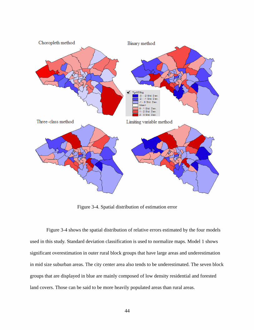
Figure 3-4. Spatial distribution of estimation error

Figure 3-4 shows the spatial distribution of relative errors estimated by the four models

used in this study. Standard deviation classification is used to normalize maps. Model 1 shows

significant overestimation in outer rural block groups that have large areas and underestimation

in mid size suburban areas. The city center area also tends to be underestimated. The seven block

groups that are displayed in blue are mainly composed of low density residential and forested

land covers. Those can be said to be more heavily populated areas than rural areas.

45

However, these areas tend to be underestimated because their areas are smaller than rural

areas, and their population density values are not as high as those of high density residential area.

This problem is because the choropleth approach does not take into account various land cover

types within units, but uses only area information to compute population density. In contrast, the

dasymetric methods compute population density with concern about the variation of land cover

types within units.

DISCUSSION AND CONCLUSION

This study has shown that the dasymetric methods are viable approaches to take into

account the underlying statistical surface from spatial data that are aggregated and attributed to

large areal units. The process may seem laborious to some geographers for mapping population

density because urban core areas typically show the same distributions. However, in large block

groups with sparse population, the dasymetric map demonstrates an intuitive and more

informative distribution. The inclusion of enhanced ancillary data can improve accuracy within

all land cover types, owing to the identification and elimination of all areas with zero population.

There are significant differences in accuracy between the choropleth method and the other three

dasymetric methods tested in this study. The limiting variable method produces a better

estimation result than the other methods in terms of RMSE. The success of the limiting variable

method may be due to its customized approach. Threshold values used to shift data between

zones are based on the data distribution for a mapped variable.

This approach contrasts with three-class method, in which the same 70-20-10 percentage

weightings are applied. The arbitrary percentage assignment of the three-class method is why the

method performs worse than other dasymetric methods. For addressing the weakness of the

46

three-class method, Mennis (2003) proposes empirical sampling strategy to determine

appropriate percentage assignment values. This technique mitigates the subjectivity of the

assignment of a percentage of population to a given ancillary data class (i.e., land use or urban

land cover). Also important are methods of determining the limiting variable threshold values.

Perhaps the reassignment schemes used for limiting variable method could also be made less

arbitrary and more specific to the geography of each source zone by making the threshold

dependent on the land cover characteristics within each source zone. For example, a threshold of

50 people per km2 used for commercial / industrial areas could be increased to 100 in tracts with

more than 50 percent urban land uses. A standardized and generalized decision process with a

statistical basis needs to be developed for this purpose.

47

REFERENCES

Burt, J. E., and G. M. Barber. 1996. Elementary Statistics for Geographers. New York: Guilford

Press.

Dorling, D. 1993. Map Design for Census Mapping. Cartographic Journal 30:167-183.





Goodchild, M. F. 1992. Geographical Data Modeling. Computers and Geosciences 18 (4):401-

408.

Holloway, S. R., J. Schumacher, and R. L. Redmond. 1999. People and Place: Dasymetric

Mapping Using ARC/INFO. In GIS Solutions in Natural Resource Management, ed. S.

Morain, 283-291. Santa Fe, NM.: Onword Press.



Slocum, T. A., and S. L. Egbert. 1993. Knowledge acquisition from choropleth maps.

Cartography and Geographic Information Systems 20 (2):83-95.

Vogelmann, J. E., T. L. Sohl, P. V. Campbell, and D. M. Shaw. 1998. Regional Land Cover

Characterization Using Landsat Thematic Mapper Data And Ancillary Data Sources.

Environmental Monitoring and Assessment 51:415-428.



48

CHAPTER 4

PYCNOPHYLACTIC INTERPOLATION REVISITED: INTEGRATION WITH

DASYMETRIC MAPPING METHOD 3

3 Kim, H. and X. Yao. Submitted to International Journal of Remote Sensing, 6/10/2009.

49

ABSTRACT

Dasymetric mapping and pycnophylactic interpolation method have solid theoretical

foundations and empirical support in population estimation research. Each of the methods has its

own strength but also suffers obvious shortcomings. In this paper, we develop a hybrid approach

that takes advantage of the strengths of both methods while overcoming their drawbacks. The

hybrid method is tested with a case study. To evaluate the performance of the proposed hybrid

method, this study compares its estimation accuracy with those of other popular methods

including areal weighting interpolation, binary dasymetric mapping, and pycnophylactic

interpolation method. The comparison results prove that the proposed hybrid method

significantly outperforms the other methods. In addition, the study conducts a sensitivity analysis

to examine the effect of search radius size, which is the key parameter of the hybrid method, on

estimation accuracy. The analysis result shows that the hybrid method can be further improved

with appropriate choice of search radius. Keyword: dasymetric, pycnophylactic, population

50

INTRODUCTION

Availability of high precision population data is one of the most important factors in

many decision making processes to address numerous spatial problems. Examples range from

site location for business development, public health (Hay et al. 2005; Langford and Higgs 2006),

to inland security issues such as emergency contingency plans (Dobson et al. 2003; Garb et al.

2007). Decennial censuses have been the primary source of spatio-demographic information.

However, to protect confidentiality and for other reasons, census data are released only as

spatially aggregated attributes of census units such as county, census tract, block group, and

block. The recently launched American Community Survey (ACS) is planning to release annual

population estimates. Although the much improved frequency of data collection and release is

well worth praising, the ACS data have even coarser spatial granularity which significantly limits

its usability for many studies. The finest ACS data are aggregated at the county level for most

areas. This coarse spatial granularity of available population data imposes many limitations and

barriers of application. For example, researchers and practitioners need to take caution against

ecological fallacy and modifiable area unit problems when using such spatially aggregated data.

Furthermore, the census enumeration units may not be compatible with some other areal units for

which other spatial data are collected, which creates problems for spatial data integration. A

common solution is to interpolate spatially aggregated population data into a different spatial

zoning system or a raster system of higher spatial resolution, which falls in the research field of

population interpolation and estimation.

Research on population estimation has been generally classified into two categories:

areal interpolation and statistical modeling (Wu et al. 2005). The statistical modeling approach

employs statistical methods such as regression model to estimate total population based on

51

urban morphological or socioeconomic indicators instead of census data (Lo 1986). Examples of

these morphological indicators include the extent of built-up and other areas that can be extracted

from remotely sensed data. Although statistical modeling methods are appropriate when census

data are not available, they produce essentially the same type of spatially aggregated population

counts with coarse spatial granularity. Therefore they share the same weaknesses as discussed

earlier.

To investigate local variations of population distribution and to estimate population data

of higher spatial granularity, many prior studies have explored the areal interpolation approach

for population estimation. Areal interpolation refers to the process of transferring data from one

set of areas (source zones) to another (target zone) (Lam 1983). For instance, it can be the

process of disaggregating population counts of census zones to smaller spatial units such as

raster grid cells. Spatial interpolation methods for population estimation can be further classified

according to whether ancillary information is utilized (Wu et al. 2005). The simplest areal

interpolation approach without ancillary information is probably the areal weighting method

which assumes population is uniformly distributed within each source zone. Many studies are

found in the literature that aim to overcome the oversimplified ‘uniform distribution’ assumption

by smooth density functions, for instance, using a kernel-based surface function around

population centroids (Bracken 1989; Bracken and Martin 1989; Martin 1989, 1996). A well-

known example of this is Tobler’s (1979) pycnophylactic method. This method replaces the

uniform distribution assumption by a smooth density function extending to adjacent source zones

while preserving its original volume (count) of each zone. More recently, the type of spatial

interpolation that integrates ancillary information has gain more visibility. This type of method is

commonly called the dasymetric mapping method. Since Wright (1936) introduced the

52

dasymetric mapping method with a rather loose definition, many researchers elaborate the

method with specifics in various studies (Eicher and Brewer 2001; Langford 2003; Mennis 2003;

Langford 2006; Mennis and Hultgren 2006). The basic principle of dasymetric mapping remains

as simple as subdividing source zones into smaller spatial units that possess greater internal

consistency in population distribution (Langford 2003). The ancillary data are usually spatially

referenced categorical information that helps to shed light on more detailed variations of

population density within source zones. For instance, the ancillary information is classified

remote sensing data revealing residential locations (cells), thus population counts can be re-

distributed to the residential cells only.

Although both types of fine-grained areal interpolation methods have solid theoretical

foundation and empirical support, each of the methods has its own strength and shortcomings.

Dasymetric mapping makes good use of ancillary information to infer most likely population

distribution, while the limitation lies in its assumption of uniform distribution of population

among all eligible locations. The pycnophylactic interpolation warrants a smooth population

surface in the study area without any presumption of uniform distribution. However, the

pycnophylactic method does not draw on information about real population distribution so that

its estimation accuracy cannot benefit from such information. It is interesting to see that the

advantages and shortcomings of the two methods are complementary to each other. With

particular interest in high resolution population estimation, this study focuses on the interpolation

type of population estimation. The objective of this study is to develop a population interpolation

method that combines the strengths of both dasymetric mapping and pycnophylactic

interpolation while overcoming the shortcomings of both.

53

The rest of the manuscript is organized as follows. The next section provides a review of

literature on the population interpolation with critiques for each method. Section 3 presents a

new hybrid approach, conducts a case study using the reviewed methods and our hybrid method,

evaluates and compares all methods, and finally performs a sensitivity analysis to examine the

impact of parameter choices on estimation results. The manuscript concludes with a summary of

research findings and a discussion of possible further research avenues.

AREAL INTERPOLATION FOR POPULATION ESTIMATION

Areal interpolation and dasymetric mapping

Areal interpolation concerns the transformation of geographic data from one zonation of

a region to another (Fisher and Langford 1995). The problem of population estimation from

aggregated census levels to more disaggregated areas is areal interpolation of population counts

(Mennis 2003). The traditional areal weighting method is the most straightforward areal

interpolation approach that can be easily implemented (Lam 1983; Flowerdew and Green 1992;

Goodchild et al. 1993). The method simply allocates a fraction of population count in a source

zone to a target zone by the proportion of the target zone overlapping the source zone. The major

flaw of this method is the oversimplified assumption that people are evenly distributed within

each source zone. This assumption is unfounded and generally inaccurate but acceptable if

nothing else is known about the population distribution (Fisher and Langford 1996). Various

methods have been proposed to overcome the fundamental flaw of the areal weighting method.

The increasing availability of remotely sensed imagery, which is able to reveal detailed

distribution of residential areas (Holt et al. 2004), has driven much of recent research on

population interpolation using dasymetric mapping method. Many researchers find that

54

dasymetric mapping gives the best estimation result among those by all other popular methods

tested (Fisher and Langford 1995; Cockings et al. 1997; Mrozinski and Cromley 1999).

The original definition of dasymetric mapping provides a general idea with no specific

rules for implementation. Basically, the method aims to utilize any available spatial information

that can provide further insight into the probable structure of source zones and thus can be

informative for redistributing population counts (Langford 2003, 142). Regarding the data source

for ancillary information, classified remotely sensed imagery has been commonly used, although

there are also several exceptions such as street networks (Xie 1996; Mrozinski and Cromley

1999; Reibel and Bufalino 2005) and rasterized topographic maps (Langford 2007).

The simplest scheme for implementing dasymetric mapping with remotely sensed data is

to use a binary mask of land cover types. The binary mask has pixels classified as, for instance,

occupied or unoccupied. Census population counts are then redistributed to those occupied pixels

only (Langford and Unwin 1994; Fisher and Langford 1996; Holt et al. 2004). It is also possible

to use more than two land cover classes for more detailed land cover information (Langford et al.

1991; Yuan et al. 1997; Eicher and Brewer 2001; Mennis 2003) as long as the way to determine

population density for each land cover class are defined. For example, Eicher and Brewer (2001)

used pre-defined population density statistics. Others used regression analysis to derive

population density estimates for each class (Langford et al. 1991; Yuan et al. 1997). There are

also studies applying empirical sampling results (Mennis 2003; Mennis and Hultgren 2006) to

establish the relationship between density values and land use land cover classes. However,

regardless of the method in use, there is little evidence that shows any clear benefit of the multi-

class method over the simpler binary dasymetric method (Langford and Higgs 2006).

55

Although the dasymetric mapping method is a favorable areal interpolation method due

to its superior performance over others, it has several methodological and cartographical

shortcomings. First, uniform distribution is still assumed among pixels of the same land use land

cover type. As a result, abrupt changes of population density can be found at borders of source

zones and those between different land use land cover types. Secondly, there is a conceptual flaw

with the population density calculation used in dasymetric mapping. Population is discrete in

nature, however population density is not. Dixon (1972) argued that population density cannot be

observed at a point. Without referring to an area over which it is evaluated, population density at

a point does not make any sense. One may argue that a pixel in the land cover map derived from

a remotely sensed imagery can be regarded as a small areal unit with the size equivalent to its

spatial resolution. However, the area is too small to completely justify the true meaning of

population density as a per-pixel value. Suppose there are two adjacent pixels with different land

use land cover classes, the contrast between the two neighboring cells could be mistakenly

exaggerated due to the flaw of this rather discrete measure of population density. The above two

shortcomings also brings about cartographic and visualization limitations. As argued by

Langford and Unwin (1994), a population density map produced by dasymetric mapping is not

suitable for cartographic purposes.

In response to these problems, Langford and Unwin (1994) suggested applying simple

low-pass filtering operation to the initial output of dasymetric mapping. The solution adds a

smoothing effect and allows for effective isarithmic or pseudo-three-dimensional representation.

Using a given radius, Langford and Unwin (1994)’s method uses a floating circular window of

the given radius over each point of the study area. It replaces population density at every point

with the average density in the floating window when the center of the circular window is on the

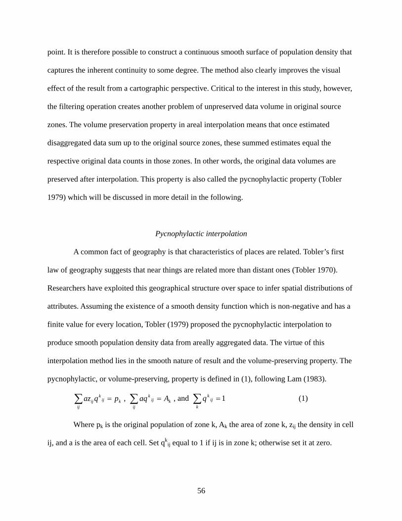
56

point. It is therefore possible to construct a continuous smooth surface of population density that

captures the inherent continuity to some degree. The method also clearly improves the visual

effect of the result from a cartographic perspective. Critical to the interest in this study, however,

the filtering operation creates another problem of unpreserved data volume in original source

zones. The volume preservation property in areal interpolation means that once estimated

disaggregated data sum up to the original source zones, these summed estimates equal the

respective original data counts in those zones. In other words, the original data volumes are

preserved after interpolation. This property is also called the pycnophylactic property (Tobler

1979) which will be discussed in more detail in the following.

Pycnophylactic interpolation

A common fact of geography is that characteristics of places are related. Tobler’s first

law of geography suggests that near things are related more than distant ones (Tobler 1970).

Researchers have exploited this geographical structure over space to infer spatial distributions of

attributes. Assuming the existence of a smooth density function which is non-negative and has a

finite value for every location, Tobler (1979) proposed the pycnophylactic interpolation to

produce smooth population density data from areally aggregated data. The virtue of this

interpolation method lies in the smooth nature of result and the volume-preserving property. The

pycnophylactic, or volume-preserving, property is defined in (1), following Lam (1983).

∑ =ij

kijk

ij pqaz , ∑ =ij

kijk Aaq , and ∑ =

kij

kq 1 (1)

Where pk is the original population of zone k, Ak the area of zone k, zij the density in cell

ij, and a is the area of each cell. Set qkij equal to 1 if ij is in zone k; otherwise set it at zero.

57

The interpolation procedure begins by assigning the mean density to each grid cell

superimposed on the source zones, and then modifies the assigned values by slight amounts to

bring the density closer to the value required by the governing partial differential equation

(Tobler, 1979).

Where, Ri denotes the ith region and Hi is the total population count in region i. The

volume-preserving condition is then enforced by either incrementing or decrementing all the

density values within individual zone at the end of each iteration. To elaborate the details, the

procedure may consists of six steps: 1) overlay a high resolution raster grid system over the study

area; 2) divide each source zone's total value equally among the raster cells that fall within the

zone; 3) smooth the values by replacing each cell's value with the average in its neighborhood;

4) sum the values of the cells in each zone; 5) adjust the values of all cells within each zone

proportionally so that the zone's total is the same as the original total. For instance, if the total is

10% lower than the original zonal total, increase the value of each cell by 10%; and 6) repeat

steps 3, 4 and 5 until no more changes are necessary. As Lam (1983) noted, the choices of an

appropriate smooth density function and of a search window size heavily depend on the

characteristics of individual applications.

∫∫ =iR

iHdxdyyxZ ),( (2)

58

A HYBRID APPROACH FOR POPULATION ESTIMATION

Summarizing the literature review and critique on popular population interpolation

methods, it is interesting to find that dasymetric and pycnophylactic method have

complementary strengths and shortcoming for population estimation. The dasymetric mapping

method is regarded as the most accurate interpolation approach among all tested popular

methods (Wu et al. 2005). It is not surprising because this method has particular strength of

making use of additional information revealing useful spatial structure of the study area.

However, it does have the drawback of unfounded assumption of uniform distribution among

eligible pixels and the conceptual flaw in calculating population density. The pycnophylactic

method presents conceptual improvements because spatial continuity is assumed and

incorporated so that a more realistic, smooth density surface can be produced. Meanwhile it also

has the desired volume-preserving quality. The major limitation of pycnophylactic method is the

lack of additional supporting information that reveals the real world spatial structure of the study

area. Interestingly, this limitation happens to be the strength of dasymetric mapping method.

Therefore, this study proposes a hybrid pycnophylactic-dasymetric method to take advantage of

the strengths and overcome the weaknesses of both methods.

The Hybrid method and research design

The general steps of the hybrid pycnophylactic-dasymetric interpolation method are

illustrated in Figure 4-1. It consists of two consecutive steps, the dasymetric mapping for a

preliminary population re-distribution and an iterative pycnophylactic interpolation process for a

volume-preserved smoothed surface. We choose binary dasymetric mapping because prior

studies found no evidence to support any extra benefits of using multi-class dasymetric mapping.

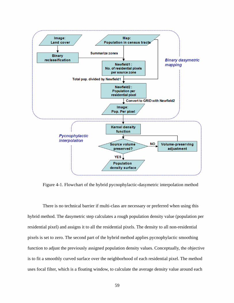
59

Figure 4-1. Flowchart of the hybrid pycnophylactic-dasymetric interpolation method

There is no technical barrier if multi-class are necessary or preferred when using this

hybrid method. The dasymetric step calculates a rough population density value (population per

residential pixel) and assigns it to all the residential pixels. The density to all non-residential

pixels is set to zero. The second part of the hybrid method applies pycnophylactic smoothing

function to adjust the previously assigned population density values. Conceptually, the objective

is to fit a smoothly curved surface over the neighborhood of each residential pixel. The method

uses focal filter, which is a floating window, to calculate the average density value around each

60

output pixel. The size of the floating window is called search distance. This search distance is

user-defined and is the key parameter in the method. We use the focal statistics tool provided by

ESRI ArcGIS® 9.3. A fundamental requirement of pycnophylactic approach is volume-preserving.

This process is designed to be an iterative process of fine-tuning until the integral of smoothed

density values in the source zone matches the original value of source zone. Finally, a smooth

population surface dataset is obtained from the interpolation result. As such, the hybrid method

makes use of ancillary information that shed lights on the population distribution and also adopts

conceptually more plausible calculation of population density by implementing smoothed

transition of densities over neighborhoods. Therefore, it benefits from the strength of both

methods and overcomes their weaknesses.

Figure 4-2 shows the overall research design of this study to carry out and evaluate the

proposed method. The input data are the same as that of dasymetric mapping, including the

aggregated census population data and classified land cover data from remote sensing imagery.

Four methods of population interpolation methods, including the proposed hybrid method and all

three popular methods are critiqued in the literature review section. Each of these methods is

applied independently. We follow procedures of the three existing methods as described in the

literature review section and the procedure of the hybrid method as discussed earlier in this

section.

61

Figure 4-2. Research Design

Once the results of all three methods are out, these results will be evaluated against each

other for a comparison of the methods’ performances. Our hypothesis is that the hybrid method

will output perform the other methods. One of the major obstacles to the evaluation of estimation

result is the absence of definitive high resolution population data to compare with. To deal with

this problem, this study aggregates the estimated population surface data to a census spatial level

that is finer than that of the original source data. The census population counts at this finer spatial

level are then used as ground truth data for the evaluation of estimation performance. In this

study, we choose census population at the block group level as ground truth data. The process

also involves an accuracy assessment component as shown in Figure 4-2. We use both the root

mean squared error (RMSE) and the mean absolute percent error (MAPE) to measure the overall

62

accuracy for each method. In addition, to investigate the effect of the choice of the key parameter,

the size of search radius, on the estimation accuracy, the study carries out a sensitivity analysis

on this parameter.

All tasks in the research design are developed in a GIS environment. In this study, we

used ERDAS Imagine® 9.2 and ESRI ArcGIS® 9.3 for converting vector population map to GRID

format and other processing of the spatially referenced population data. The pycnophylactic

interpolation and hybrid dasymetric mapping method developed in this study were implemented

by Python2.4® script in the ArcGIS environment.

Case Study

A case study is carried out according to the research design. The study area is the Atlanta

Metropolitan Statistical Area (MSA) in Georgia. As shown in Figure 4-3, the study area

encompasses 28 counties with diverse land use land cover types. It has a total population of over

4 million according to the 2000 national census. Input data includes the 2000 population census

at census tract level, and the 1998 land cover map (Figure 4-4) acquired via Georgia GIS Data

Clearinghouse (http://www.gis.state.ga.us) as ancillary information. In addition, we use the U.S.

Census Bureau’s 2000 census population data at block group level as ground truth data for

accuracy assessment of estimated population data.

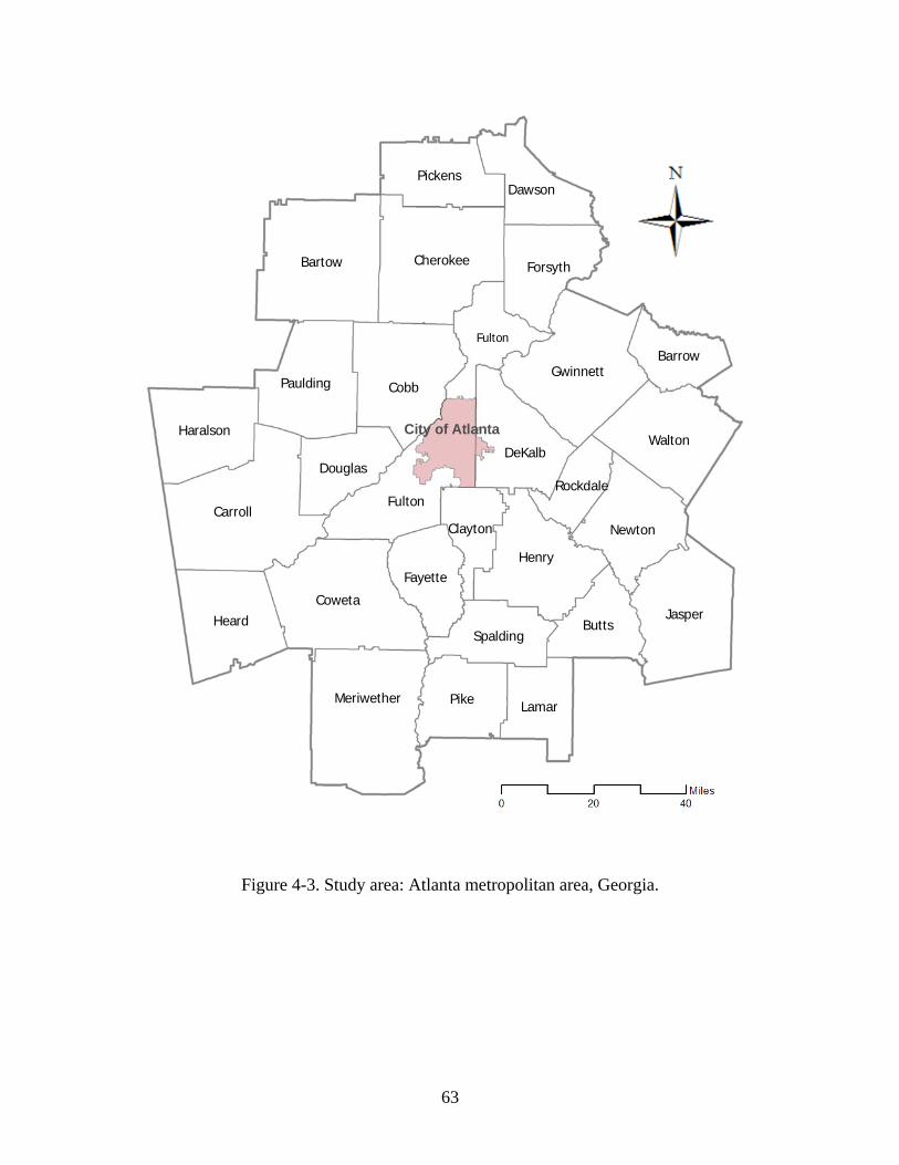
63

City of Atlanta

Fulton

Meriwether

FultonCarroll

Cobb

Bartow

CowetaJasper

Henry

Pike

Heard

Gwinnett

Walton

Cherokee

DeKalb

Paulding

Butts

Newton

Forsyth

Haralson

Pickens

Lamar

Fayette

Dawson

Douglas

Spalding

Barrow

Clayton

Rockdale

Figure 4-3. Study area: Atlanta metropolitan area, Georgia.

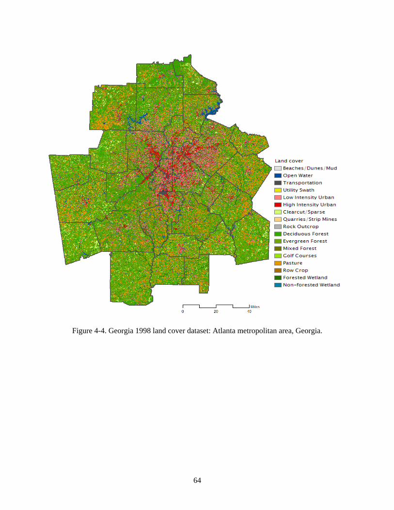
64

Figure 4-4. Georgia 1998 land cover dataset: Atlanta metropolitan area, Georgia.

65

The study area of 690 census tracts or 1,923 block groups covers a wide range of

landscapes. There are highly populated urban areas, low density suburbs, forests, vacant lands,

and agriculture land, as shown in the image of land cover map in Figure 4-4. The land cover

dataset was produced by the Natural Resource Spatial Analysis Laboratory at the University of

Georgia using leaf-off Landsat TM images taken between 1996 and 1998. Two classes in the

classified image are associated with residential land use. They are the low intensity urban and

high intensity urban as described in Table 4-1. The problem is developed land cover classes are

associated with not only residential land use but also other urban land uses including commercial,

industrial, leisure, transportation, and so on. Isolating residential land use from other urban land

uses could be one of the best ways to enhance the accuracy of dasymetric method. However, it is

a practically impossible or at least extremely time-consuming task, if possible at all. In this

research, we reclassified the land cover data to make a binary mask of residential area assuming

that all urban pixels are eligible for population distribution in the dasymetric mapping step.

Table 4-1. Urban land cover classes of the land cover dataset

Code Class Name Description

22 Low Intensity Urban

This class includes; single family residential areas, urban recreational areas, cemeteries, playing fields, campus-like institutions, parks, and schools.

24 High Intensity Urban

This class includes central business districts, multi-family dwellings, commercial facilities, industrial facilities, and high impervious surface areas of institutional facilities.

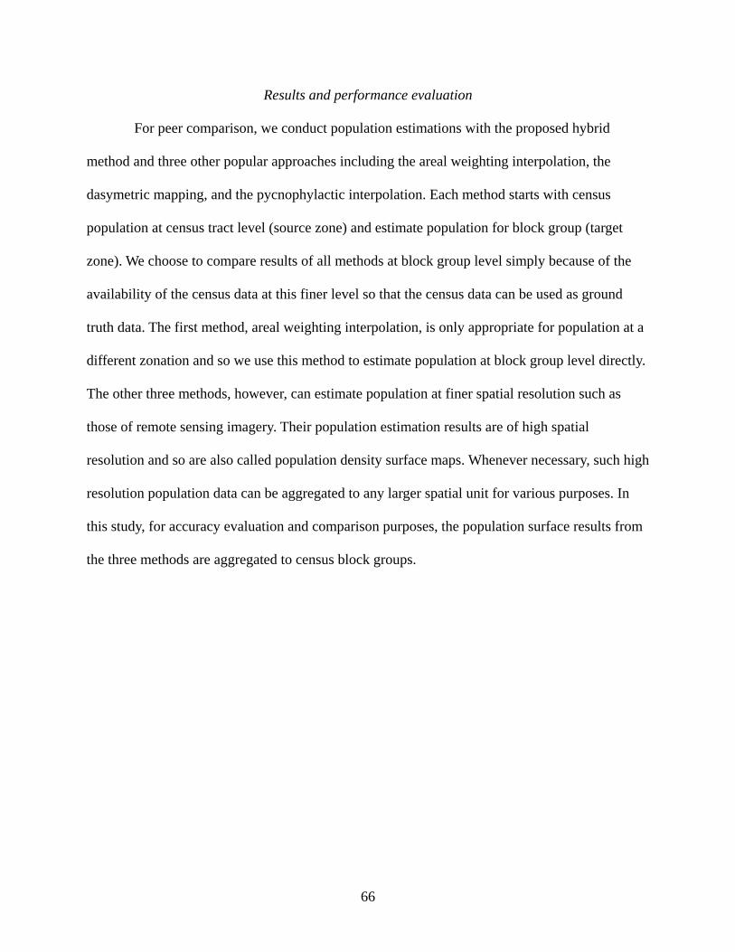
66

Results and performance evaluation

For peer comparison, we conduct population estimations with the proposed hybrid

method and three other popular approaches including the areal weighting interpolation, the

dasymetric mapping, and the pycnophylactic interpolation. Each method starts with census

population at census tract level (source zone) and estimate population for block group (target

zone). We choose to compare results of all methods at block group level simply because of the

availability of the census data at this finer level so that the census data can be used as ground

truth data. The first method, areal weighting interpolation, is only appropriate for population at a

different zonation and so we use this method to estimate population at block group level directly.

The other three methods, however, can estimate population at finer spatial resolution such as

those of remote sensing imagery. Their population estimation results are of high spatial

resolution and so are also called population density surface maps. Whenever necessary, such high

resolution population data can be aggregated to any larger spatial unit for various purposes. In

this study, for accuracy evaluation and comparison purposes, the population surface results from

the three methods are aggregated to census block groups.

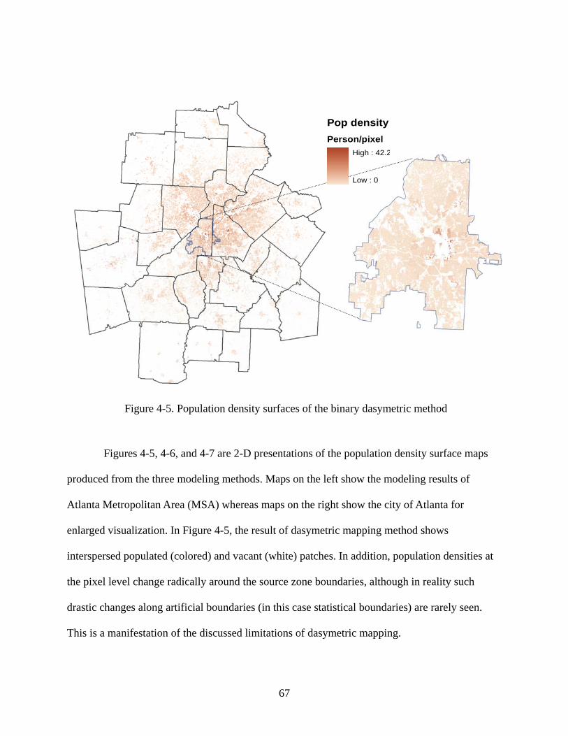
67

Figure 4-5. Population density surfaces of the binary dasymetric method

Figures 4-5, 4-6, and 4-7 are 2-D presentations of the population density surface maps

produced from the three modeling methods. Maps on the left show the modeling results of

Atlanta Metropolitan Area (MSA) whereas maps on the right show the city of Atlanta for

enlarged visualization. In Figure 4-5, the result of dasymetric mapping method shows

interspersed populated (colored) and vacant (white) patches. In addition, population densities at

the pixel level change radically around the source zone boundaries, although in reality such

drastic changes along artificial boundaries (in this case statistical boundaries) are rarely seen.

This is a manifestation of the discussed limitations of dasymetric mapping.

Pop densityPerson/pixel

High : 42.2

Low : 0

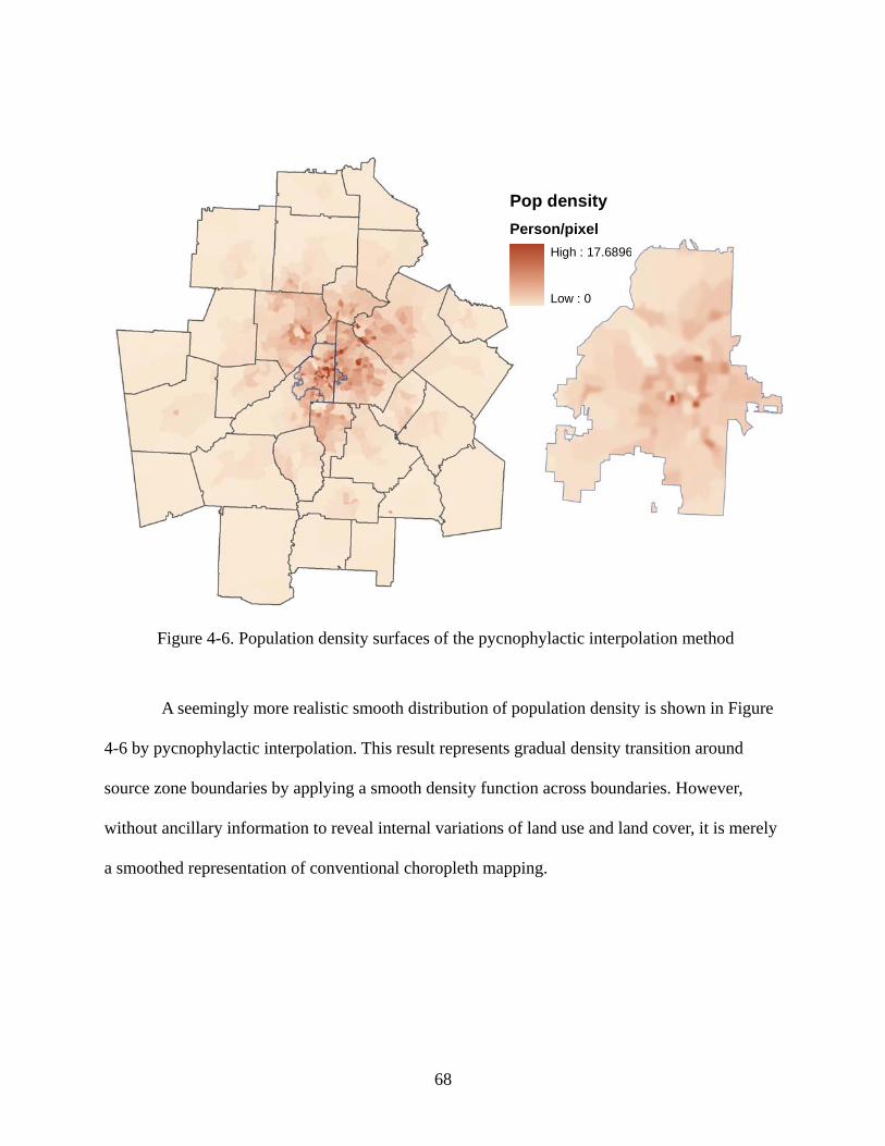
68

Figure 4-6. Population density surfaces of the pycnophylactic interpolation method

A seemingly more realistic smooth distribution of population density is shown in Figure

4-6 by pycnophylactic interpolation. This result represents gradual density transition around

source zone boundaries by applying a smooth density function across boundaries. However,

without ancillary information to reveal internal variations of land use and land cover, it is merely

a smoothed representation of conventional choropleth mapping.


High : 17.6896

Low : 0

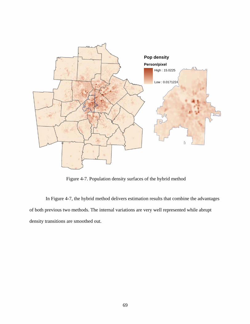
69

Figure 4-7. Population density surfaces of the hybrid method

In Figure 4-7, the hybrid method delivers estimation results that combine the advantages

of both previous two methods. The internal variations are very well represented while abrupt

density transitions are smoothed out.


High : 15.0225

Low : 0.0171224

70

Table 4-2 compares the estimation accuracy of all methods tested. The four methods are

put in two categories. One category has the two methods using ancillary information, while the

other category has methods that do not use any additional information. For each method, two

measures are calculated for accuracy assessment. The first is the root mean squared error

(RMSE) defined in Equation (3). The second measure is the mean absolute percent error

(MAPE) defined in Equation (4).

n

PPRMSE

n

jajej∑

=

−= 1

2)( (3)

n

PPPMAPE

n

jajajej∑

=

−= 1

/)(

(4)

Where Pej is the estimated population of the jth target zone; Paj is the actual census

population of the jth target zone; and n is the total number of target zones.

Table 4-2. Estimation accuracy results from four interpolation methods

Interpolator

Without ancillary information With ancillary information

Areal weighting Simple pycnophylactic

Binary dasymetric Hybrid method

RMS error 941 916 769 745

MAPE (%) 37.21 35.14 28.59 26.58

Note: total target zones N=1923, mean population of target zones = 6156

71

Several interesting findings are observed in Table 4-2. First, the advantage of using

ancillary information in population estimation is evident. Whether ancillary information is used

in the method becomes a natural divider to categorize them according to the estimation accuracy.

Secondly, between the two methods using ancillary information, the hybrid method clearly

outperforms the dasymetric method in both measures. Thirdly and not surprisingly, the areal

weighting interpolation gives the most inaccurate results, which is consistent with findings in the

literature. Finally, the proposed hybrid method gives the most accurate estimation.

Sensitivity analysis and optimization of search radius

Inherited from the conventional pycnophylactic interpolation, the hybrid method

imposes a moving window around each pixel when applying the smoothing kernel function. It is

important to investigate the effect of the varying window sizes and to find optimal radius of the

search window. Among the four tested methods, only the hybrid and the pycnophylactic

interpolation methods require the parameter of search radius. In the initial experiment that was

reported in Table 4-2, the search radius is arbitrarily chosen to be 90 meters, which is the size of

three pixels, for both methods. How sensitive are the results of these methods to the search

radius? More importantly, how sensitive is the comparative advantage of the hybrid method to

the parameter? We conduct a sensitivity analysis to answer these questions. Population

estimations were conducted repeatedly with varying search radii for both applicable methods. We

start with a small search radius, 90 meters. Then the radius gradually increases by 30 meters (one

pixel) each time. Figure 4-8 plots the relationship between search radius and the RMS error of

the estimation result for both methods. It clearly shows that both methods are sensitive to the

choice of search radius. The estimation accuracies of both the hybrid method and the

72

pycnophylactic method can be significantly improved by appropriate choice of the search radius.

The hybrid method consistently outperforms pycnophylactic interpolation regardless of the

search radius in use. In fact, the difference in RMS errors of the two methods can be as large as

80, roughly 10% of the RMS error. It is also found that the two methods reach optimal search

radius at a different point. For the hybrid method, the optimal search radius is roughly in the

range between 630 to 690 meters, while pycnophylactic method has its optimal search radius at

about 900 meters.

Figure 4-8. Effect of search radius in the population distribution estimation error

73

DISCUSSION AND FURTHER RESEARCH

Based on a careful examination of the strength and shortcomings of some popular areal

interpolation methods for population estimation, this study proposes a hybrid method that takes

advantages of both dasymetric mapping and pycnophylactic interpolation. The hybrid method

combines the strength and overcomes the weaknesses of both previous methods. Although we

present the method with specific focus on population estimation, the principle of the hybrid

approach is applicable to areal interpolation in general. Using classified high spatial resolution

land use and land cover data as ancillary information, the hybrid method disaggregates zone-

based census population data to high resolution population raster data. Such data can be

visualized as surface of population distribution. The case study validates and tests this proposed

method along with several other popular methods for comparative evaluation. The comparison

suggests several findings. Firstly, the methods using ancillary information give significantly

better estimate accuracy than those that do not use any of such information. This finding suggests

that remote sensing data and techniques are key elements to the quality of high resolution

population estimation. Secondly, the proposed hybrid method is the best among all other tested

approaches. Thirdly, it is found that estimation accuracy of any method that uses a smoothing

kernel density function parameterized by search radius is sensitive to the size of the search radius.

However, regardless of the size in use, the hybrid method shows consistent competitive edge

over the other tested methods. In summary, the proposed hybrid method is proven to be a

promising method that shows theoretical and accuracy advantage over other currently popular

methods.

During the course of this study, we have reflected on several issues regarding the quality

of population estimation, particularly concerning spatial precision and estimation accuracy. Some

74

of the issues remain open for further investigation. For population estimation methods (a typical

example is dasymetric mapping) that employ ancillary information, many factors could affect the

estimation accuracy but the key factor is the quality of ancillary data. The most popular type of

ancillary data for dasymetric mapping is classified remote sensing images of land cover and land

use types. Currently used are pixel-based classifications which focus on electromagnetic

reflectance values of individual pixels while other context information such as shape and size of

patches of pixels, as well as relationships among those patches or pixels, are not explored.

Further research can take advantage of additional information by using, for instance, the state-of-

the-art object-based classification techniques. Another issue relates to the classification scheme.

Often a binary classification of residential versus non-residential land use is used. However, clear

distinction between residential land use and other land uses, especially other developed land uses,

is very difficult and time-consuming, hence not widely available. Instead, most publically

available land cover datasets have multiple classes of developed land use and there is no well-

qualified method to separate residential areas out of other urban land uses. Thus a time-saving

alternative solution is to enhance the accuracy of dasymetric population estimation method that

uses multiple land cover classes directly. Another research avenue is to incorporate locally varied

spatial dependence of population density into population estimation methods. Although this

study reveals optimal range of search radius, the specific numbers are hardly applicable to other

areas. Optimal size of search radius needs to be explored on a case by case basis. Similarly, it

might be even oversimplified to assume that a search size is equally suitable to all portions in the

study area. Instead, it is reasonable to assume locally varied parameters. For study areas where

population density is expected or proven spatially autocorrelated, a locally adaptive modeling

approach is theoretically more plausible and thus absolutely worth pursuing.

75

REFERENCES







Dixon, O. M. 1972. Method and progress in choropleth mapping of population density. The

Cartographic Journal 9:19-29.

Dobson, J. E., E. A. Bright, P. R. Coleman, and B. L. Bhaduri. 2003. LandScan: A global

population database for estimating population at risk. In Remotely Sensed Cities, ed. V.

Mesev, 267-279. London: Taylor & Francis.





———. 1996. Modeling sensitivity to accuracy in classified imagery: A study of areal

interpolation. Professional Geographer 48 (3):299-309.




76

Garb, J. L., R. G. Cromley, and R. B. Wait. 2007. Estimating Populations at Risk for Disaster

Preparedness and Response. Journal of Homeland Security and Emergency Management

4 (1):1-17.



Hay, S. I., A. M. Noor, A. Nelson, and A. J. Tatem. 2005. The accuracy of human population

maps for public health application. Tropical Medicine and International Health 10

(20):1073-1086.



(2):103-121.


(2):129-149.

Langford, M. 2003. Refining methods for dasymetric mapping. In Remotely Sensed Cities, ed. V.


———. 2006. Obtaining population estimates in non-census reporting zones: An evaluation of

the 3-class dasymetric method. Computers, Environment and Urban Systems 30 (2):161-

180.



Langford, M., and G. Higgs. 2006. Measuring Potential Access to Primary Healthcare Services:

The Influence of Alternative Spatial Representations of Population. Professional

Geographer 58 (3):294-306.

77







Lo, C. 1986. Applied Remote Sensing: Harlow: Longman.

Martin, D. 1989. Mapping Population Data from Zone Centroid Locations. Transactions of the

Institute of British Geographers 14 (1):90-97.

———. 1996. An assessment of surface and zonal models of population. International Journal

of Geographical Information Science 10 (8):973-989.



Mennis, J., and T. Hultgren. 2006. Intelligent Dasymetric Mapping and Its Application to Areal

Interpolation. Cartography and Geographic Information Science 33 (3):179-194.





Tobler, W. 1970. A computer movie simulating urban growth in the Detroit region. Economic

Geography 46 (2):234-240.

———. 1979. Smooth pycnophylactic interpolation for geographic regions. Journal of the


78



Wu, S., X. Qiu, and L. Wang. 2005. Population estimation methods in GIS and remote sensing: A

review. GIScience & Remote Sensing 42 (1):80-96.

Xie, Y. 1996. The Overlaid Network Algorithms for Areal Interpolation Problem. Computers,

Environment and Urban Systems 19:287-306.



(3-4):245-258.

79

CHAPTER 5

A LOCALLY ADAPTIVE INTELLIGENT INTERPOLATION METHOD FOR

POPULATION DISTRIBUTION MODELING USING PRE-CLASSIFIED LAND

COVER DATA 4

4 Kim, H. and X. Yao. To be submitted to Professional Geographers.

80

ABSTRACT

Intelligent interpolation methods such as dasymetric mapping are considered to be the

best way to disaggregate zone-based population data by observing and utilizing the internal

variations within each source zone. In this paper, we critique the advantages and problems of the

dasymetric mapping method. The paper presents a geographically weighted regression (GWR)

based method to take into consideration the spatial heterogeneity of population density - land

cover relationship. The locally adaptive intelligent interpolation method is able to make use of

readily available ancillary information in the public domain without the need for additional data

processing. In a case study, we use the pre-classified National Land Cover Dataset (NLCD) 2001

to test the performance of the proposed method compared to four other popular population

estimation methods: areal interpolation methods including areal weighting interpolation,

pycnophylactic interpolation, binary dasymetric method, and globally fitted ordinary least

squared (OLS) based multi-class dasymetric method. The GWR-based multi-class dasymetric

method outperforms all other methods. It is attributed to the fact that spatial heterogeneity is

accounted for in the process of determining density parameters for land cover classes. Keywords:

Dasymetric; Heterogeneity; Geographically weighted regression; NLCD

81

INTRODUCTION

High precision population distribution data are extremely important in numerous

decision making and real world problem solving efforts. Examples include those in business,

health, national security, and emergency response applications (Dobson et al. 2003; Hay et al.

2005; Langford and Higgs 2006; Garb et al. 2007). Population estimation often boils down to the

re-distribution of spatial aggregated census data to spaital units of finer resolution – a process of

spatial intepolation. Population interpolation refers to the process of transferring population data

from one set of spatial units (source zones) to another (target zones). The literature is replete with

various population estimation methods using spatial interpolation. According to type of

information in use, we can classify population intepolation methods into two types (Wu et al.

2005). The first type uses no additional information besides the sets of spatial units and the

population counts in one set of spatial units (the source zones). Examples include the areal

weighting intepolation (Goodchild and Lam 1980), pycnophylactic interpolation (Tobler 1979),

and kernel-based interpolation (Martin 1989). The second type of population interpolation

employs not only the above information, but also so-called ancillary inforamation with the

purpose to integrate internal variations of source zone. These types of methods are also called

‘intelligent’ interpolation methods by some people as they have a common goal of exploiting

additional relevant knowledge to generate better target zone estimates (Flowerdew and Green

1994).

Dasymetric mapping method is a typical example of those intelligent interpolation

methods. It has been increasingly popular nowadays, especially due to the emergence and

growing popularity of GIS and remote sensing technologies. Since Wright (1936) introduced the

dasymetric mapping method (although the earliest reference to dasymetric mapping is the 1922

82

population map of European Russia by Semenov Tian-Shansky according to Mennis and

Hultgren (2006)), many researchers elaborate the method with specifics in various studies. The

basic principle of dasymetric mapping remains as simple as subdividing source zones into

smaller spatial units that possess greater internal consistency in population distribution (Langford

2003). The ancillary information is typically spatially referenced GIS data layers of land cover

land use that shed light on more detailed spatial structures of population distribution.

Many studies have demonstrated that the dasymetric method can substantially improve

population estimation accuracy (Mrozinski and Cromley 1999; Langford 2006; Reibel and

Agrawal 2007). In fact, some earlier comparative studies concluded that dasymetric mapping

was the best performer among all popular population interpolation methods (Fisher and Langford

1995; Cockings et al. 1997; Mrozinski and Cromley 1999). Despite the significant performance

advantages of the dasymetric mapping, there has been little evidence to suggest widespread

adoption amongst the broader GIS community (Langford 2007). Langford (2007) stated that

intelligent methods were not widely adopted because of two reasons. First, implementation of

intelligent interpolation is much more complicated than simple areal weighting interpolation

which can be implemented by a suitable overlay tool which is readily available in most GIS

software. Furthermore, most intelligent interpolation methods require additional process to

prepare ancillary information. For instance, many researchers had to perform land use land cover

classification with satellite images to obtain ancillary data for intelligent interpolation of

population (Langford and Unwin 1994; Yuan et al. 1997; Holt et al. 2004; Sleeter 2004; Reibel

and Agrawal 2007). Areal weighting interpolation does not require the user to be involved with

the preparation of ancillary data. Moreover, these additional processing may also introduce more

errors into the original dataset because accuracy of those ancillary data is not assured and errors

83

are inherent in almost all aspects of GIS analysis. Therefore, there is no wonder that many users

still prefer the traditional simple interpolation method despite of the superior performances by

the intelligent interpolation methods reported in many studies.

There are positive and negative factors that encourage or discourage users from adopting

intelligent interpolation methods. To encourage the GIS community to employ intelligent

interpolation methods for its advantage in estimation accuracy, efforts should be made to

overcome the problems of excessive processing time and implementation difficulty. Regarding

the acquisition of high accuracy ancillary information, there are several types of high quality

datasets available in the public-domain in the United States such as the National Land Cover

Dataset (NLCD). The NLCD data are free, seamless, and intended to be updated relatively

frequently, which provides the necessary data for timely estimation. Making use of the readily

available ancillary data not only guarantees the currency of data, but also helps to minimize the

data processing time.

Methodologically, the simplest implementation scheme for dasymetric mapping with

land cover data is to use a binary mask in which land cover is classified as ‘populated’ or ‘empty’,

and census population counts are redistributed to only populated areas (Langford and Unwin

1994; Fisher and Langford 1996; Holt et al. 2004). Like simple areal weighting interpolation,

this method is conceptually simple and relatively easy to implement, and previous studies have

shown that it performs well compared to other alternatives (Martin et al. 2000; Eicher and

Brewer 2001). Another problem with the dasymetric mapping and other ‘intelligent’ population

interpolation methods is that they ignore spatial heterogeneity (or non-stationarity) in the

relationship between population distribution and the distribution of explanatory variables (e.g.

land covers). Although the current method allows spatial heterogeneity of population density

84

within each source zone by incorporating, for instance, land use land cover ancillary information,

it assumes that the relationship between the population density and any specific land use land

cover type is spatially stationary. However, in reality, such relationships may vary across space.

It is likely that a range of residential densities are present within most census reporting zones

even though the corresponding land use land cover types are the same (Langford 2006). These

differences in residential densities may arise primarily due to different housing types in the urban

areas. It is highly probable that residential areas in a city center and in a suburban town have

different population densities. This problem has been realized by many researchers who make

use of the OLS regression model in population estimation. Some attempts have been made to

deal with this problem by adopting a regional regression approach, in which the whole study area

is subdivided into smaller regions, and an OLS regression model is applied to each region to

estimate the population. Such an approach seems to produce better results for each region (Yuan

et al. 1997; Langford 2006). Albeit a good try, such a solution has obvious flaws. First, it is

difficult to know how large or small a region should be. Therefore there is no guarantee of

sufficient account of spatial heterogeneity in a study. Secondly, repeating the same process over

multiple regions in one study is tedious and deficient.

This study responds to both of the above-discussed problems of intelligent interpolation

method by introducing geographically weighted regression (GWR). The GWR method has been

designed specifically to take care of the spatial heterogeneity problem (Fotheringham et al. 2002).

We intend to examine the effectiveness of the GWR-based intelligent interpolation method in

treating spatial heterogeneity of relationships and the usefulness of the method in directly

making use of readily available multi-class land use land cover data. The remainder of the paper

is organized as follows. The next section reviews the literature on population interpolation

85

methods in general and those with consideration of the spatial heterogeneity problem in

particular. Section 3 presents the GWR-based intelligent interpolation method and carries out a

case study with it. The paper concludes in Section 4 with a summary of findings and discussions

of future work.

LITERATURE REVIEW

This paper aims to develop a multi-class dasymetric method for areal interpolation, and

evaluate its performance for cross-area estimation of population census data. To achieve this goal,

it is necessary to review other interpolation methods. Different methods have been developed to

solve the problem of spatial unit mismatch as briefly discussed above. In this section, each

method is reviewed briefly to provide a basis for performance comparison with the method we

propose.

Cross-area estimation or areal interpolation (Goodchild and Lam 1980) is primarily

designed for transferring data between two sets of non-nesting spatial units. The two spatially

incompatible data location arrays are usually termed source zone and target zone. This approach

can be divided into two categories, those that incorporate ancillary information as surrogate

variables to aid the interpolation process, and those that do not use such ancillary information.

Areal weighting interpolation

The simplest areal interpolation technique is areal weighting interpolation. The

methodology is based only on the geometric intersection of the source and target zones. It

assumes homogeneity within source zones and therefore no further ancillary information is

required to guide the interpolation process.

86

Population of each target zone is estimated by (Fisher and Langford 1995):

∑=

×=

S

s s

stst A

PAP

1

ˆ (1)

Where, S is the number of source zones; Ats is the area of overlap between target zone t

and source zone s; Ps is the population of source zone s; and As is the area of source zone s. The

technique is rather easy to implement with simple overlay and field calculation functions

available in most GIS software without any ancillary data demand. The problem with this

method is that it is incorrect to assume that population density within each source zone is

uniform. There have been numerous studies that have shown the overall low accuracy of simple

area weighting in comparison to other techniques (see for example, Mrozinski and Cromley

1999; Sadahiro 2000; Gregory 2002; Langford 2006; Reibel and Agrawal 2007))

Pycnophylactic interpolation

Pycnophylactic interpolation is probably the most quoted interpolation method, which

does not require ancillary information while denying the assumption of homogeneity within

source zones. Tobler (1979) proposed the pycnophylactic interpolation for the preparation of a

smoothed map (or isopleth map) from data collected or published in discrete areal spatial unit

system, assuming the existence of a smooth density function which is non-negative and has a

finite value for every location. The virtue of this interpolation method is that it redistributes

source zone values by distance-decay density function while ensuring original value in the

source zone intact – the so called pycnophylactic or volume-preserving property.

87

This property can be defined in (2), according to Lam (1983).

∑ =ij

kijk

ij pqaz , ∑ =ij

kijk Aaq , and ∑ =

kij

kq 1 (2)

Where, pk is the original population of zone k, Ak is the area of zone k, zij is the density in

cell ij, and a is the area of each cell. Set qkij equal to 1 if ij is in zone k; otherwise set it at 0.

The interpolation procedure begins by assigning the mean density to each grid cell

superimposed on the source zones, and then modifies the assigned values by slight amounts to

bring the density closer to the value required by the governing partial differential equation

(Tobler, 1979).

(3)

Where, Ri denotes the ith region and Hi is the total population count in region i. The

volume-preserving condition is then enforced by either incrementing or decrementing all the

density values within individual zone at the end of each iteration. Compared to the areal

weighting interpolation, the pycnophylactic method represents conceptual improvements since

the effects of neighboring source zones have been taken into account. A smoothed surface map

by pycnophylactic interpolation is also desirable for improved cartographic representation.

Pycnophylactic interpolation might be a preferred choice in the absence of any available

information about the characteristics of the surface. When such ancillary information of the land

surface is available, however, incorporating detailed land use pattern can provide a more

informed alternative to the simple distance-decay function. Ancillary information allows the

internal structure of population distribution to be inferred more explicitly. It is reasonable to

assume that people are concentrated in developed areas, especially residential areas.

∫∫ =iR

iHdxdyyxZ ),(

88

Binary dasymetric mapping

Binary dasymetric mapping is one of the simplest intelligent interpolation methods

facilitating ancillary information to infer internal structure of variables within source zones.

Dasymetric mapping was first developed as a form of cartographic representation (McCleary

1984) and is defined as a method by which source zones are subdivided into smaller subregions

that possess greater internal consistency in the densities of the variable being mapped. As the

simplest form of dasymetric mapping methods, the binary dasymetric mapping takes a binary

land use classification to control the population allocation. It assumes a non-zero density in the

populated areas within each source zone and a zero density elsewhere which is assumed as

empty. The method is different from the areal weighting interpolation as it only considers the

populated areas in the target zones for allocating population. Population of each target zone is

estimated by (Fisher and Langford 1995; Fisher and Langford 1996):

∑=

×=

S

s sp

stspt A

PAP

1

ˆ (4)

Where, S is the number of source zones; Atsp is the area of populated land cover

overlapped with both target zone t and source zone s, and ; Ps is the population of source zone s;

and Asp is the area of populated land cover within source zone s. Binary dasymetric mapping is

conceptually simple and relatively easy to implement, and performs well compared to several

alternatives according to literatures (Martin et al. 2000; Eicher and Brewer 2001; Langford 2006,

2007). It is also locally fitted to each source zone assuring volume-preserving property.

89

Multi-class dasymetric mapping

In spite of the binary dasymetric mapping allowing spatial non-stationarity of population

density within each census zone to be incorporated in the model, it is unable to address more

complex relationships between land uses and a variety of population concentration. It seems

likely that, in reality, a range of population densities will be present within most census reporting

zones (Langford 2006) by different land uses. Such differences in densities arise primarily due to

different land uses in the urban areas. It is highly probable that residential areas in a city center

and in a suburban town have different population densities.

An incremental development for the binary dasymetric method is a multi-class model

that could better accommodate the variability with different land uses, although to what extent

such complexity can be identified and modeled using ancillary information is debatable. A multi-

class dasymetric method can be algebraically represented as follows (Langford 2006):

∑∑= =

×=

S

s

C

c sc

stsct A

PAP

1 1

ˆ =∑∑= =

×S

s

C

csctsc dA

1 1 (5)

Where, S is the number of source zones; C is the number of land cover classes

accounted; Atsc is the area of land cover class c overlapped with both target zone t and source

zone s, and; Ps is the population of source zone s; Asc is the area land cover class c within source

zone s; and dsc is the dasymetric density of land cover class c in source zone s.

With implementing a multi-class dasymetric method, the most important issue is how to

calibrate density parameters for different land cover classes. With a binary dasymetric method,

population density of ‘empty’ area is fixed to zero so the density of ‘populated’ area is calibrated

by as a simple algebra as used by areal weighting interpolation. However, in a multi-class

dasymetric model, it is complicated to calibrate the density parameters for each land cover class.

Even when one land cover class, say ‘empty’, is fixed to zero, the model is mathematically

90

under-constrained and thus an infinite number of parameters exist for remaining classes. There

are several ways that are reported to overcome this difficulty, and Langford (2006) grouped them

into three groups: proportion preset, selective sampling, and statistical modeling.

Proportion preset

Eicher and Brewer (2001) assigned a fixed proportion of the total population count to

each land cover for their three-class dasymetric method. They suggested that the proportions can

be determined subjectively by using evidence collected through field survey, or from any other

suitable information source. They assigned 70% of population to urban area, 20% to

agriculture/woodland, and 10% to forested area, while no population was assigned to water

bodies.

Selective sampling

Density parameters for land cover classes can be determined by a selective sampling

strategy. Mennis (2003) isolated a number source zones filled by a single land cover class.

Assuming enough samples can be found, population density of each class is determined by

simply dividing the total population of the sampled source zone by the area. The density

parameters established in this manner are then applied to all source zones where different land

covers are present. A problem with this approach is that, in many cases, it is difficult to find

enough number of source zones filled by a single land cover class, sometimes even not at all.

With his later research (Mennis and Hultgren 2006), he proposed some other loosened sampling

methods: centroid sampling, containment sampling, and percent cover sampling.

91

Statistical modeling

A more generalized solution is to use statistical modeling (Langford et al. 1991; Yuan et

al. 1997; Langford 2006). It is generally agreed that population will most likely be found in

residential areas. With such an assumption, a single land use variable (number of populated

pixels) is usually employed to relate to population in the form of an ordinary least square (OLS)

regression model. It is also possible to relate population to a greater variety of land cover classes

in the form of a multivariate regression model, considering that population may be found in more

than one type of land cover (Langford et al., 1991). The ratios between population densities and

land cover classes are determined by a regression model, in which areas of different land cover

classes are independent variables and population count is dependent variable. In other words, it is

assumed that the given source zone population may be expressed in terms of a set of densities

related to the areas assigned to the different land cover classes. Other ancillary variables may be

included for these area densities, but the basic model is (Yuan et al. 1997):

∑=

+×=C

csSCcs AdP

1)( ε (6)

Where, Ps is the population count for each source zone s; c is the land cover class; Asc is

the area for each land class within source zone s; dc is the coefficient of the regression model;

and sε is the random error.

92

Spatial heterogeneity problem

Several issues need to be handled to apply density parameters determined by a statistical

modeling to areal interpolation methods such as dasymetric mapping. First of all, density

parameters of a regression model need to be adjusted by each source zone before they can be

used for multi-class dasymetric mapping. Regardless of how many independent variables are

used in the model, it is impractical to establish a perfect regression model (i.e. with coefficient of

multiple determinations (R2) equal to 1). And, because the density parameters are derived from a

global context, they remain stable throughout the study area. To ensure that the populations

reported within target zones are constrained to match the overall sum of the source zones (the

pycnophylactic property), the globally estimated density parameters need to be locally adjusted

within each source zone by the ratio of the predicted population and census counts.

The locally fitted approach was introduced by Yuan et al. (1997) to improve the

reliability of estimated densities derived from the regression model. The mathematical

expression of the density-adjusting approach is:

cs

scs d

PP

d ×= ˆ (7)

Where, dcs is the specific density estimates for class c in zone s; Ps is the actual

population of source zones s; sP̂ is the estimated population of source zone s; and dc is the

initial global density estimate of land class c.

93

The use of locally fitted regression has modified the assumption of the regression model

by objectively allowing spatially inconsistent density values within each land class. This

approach is comparably simple, but based on the relaxed homogeneity assumptions regarding

density. Another problem of OLS regression model refers to spatial heterogeneity. OLS

regression models are all global models, which produce one set of density parameters to apply to

the whole study area. Recent research by Langford (2006) revealed the presence of spatial

heterogeneity in the relationship between population and land cover, for which the global

regression models cannot handle. According to Fotheringham et al. (2002), heterogeneity refers

to the fact that unlike physical laws, measurement of social processes tends to vary according to

where it is made. In the case of spatial processes, it is referred to as spatial heterogeneity, or in

other words, the relationship measurements tend to vary over space.

For population estimation, the OLS regression model assumes that there exists a

stationary relationship between population and land cover. Unfortunately, this is not true because

the land use land cover extracted from the satellite images cannot be 100% accurate and spatial

variability of classification errors occurs (Lo 2008). When we try to implement multi-class

dasymetric mapping with a pre-classified land cover data such as NLCD 2001 (Note that it is

land cover data not land use data), we have to bear in mind that land cover is not directly

associated with land use. Satellite images depict land cover such as man-made structures, water,

bare soil, trees, etc. Land use should be interpreted using the land cover information and many

other components such as shape, size, and association of the land cover. That is probably why

most agencies produce land cover data rather than land use. Land cover is more objective and

easy way to present their product. In fact, different land uses could be conjectured from a single

land cover dataset depending on the procedure that was used and who did the interpretation.

94

The NLCD 2001 does not explicitly represent how the land is used. It only shows if it is

developed and how much it is developed (open, low, medium, and high intensity). It provides

some information about what land uses might be associated with each land cover categories. For

example, high intensity developed pixels might be apartment complexes, row houses, and

commercial/industrial without saying what exactly it is. It is highly probable that pixels with the

same land cover class might have different land uses according to where the pixel is located.

Hence, a density parameter for each land cover class might vary spatially as well. All these give

rise to spatial heterogeneity, which the OLS model cannot address.

Such a problem has been realized by many researchers who make use of the OLS

regression model in population estimation. Some attempts have been made to deal with this

problem by adopting a regional regression approach, in which the whole study area is subdivided

into smaller regions, and an OLS regression model is applied to each region to estimate the

population. Such an approach seems to produce better results for each region (Yuan et al. 1997;

Huang and Leung 2002; Langford 2006). However, it is difficult to know how large a region

should be. Yuan et al. (1997) made use of counties as regions. This seems to produce good

population estimates for each county. However, this model also suffers from the same problem

of spatial heterogeneity as discussed above. The accuracy of a population–land use model for

population estimation does not depend totally on the independent variables used or any other

ancillary data included. It appears that a local rather than a global approach is needed to deal

with the spatial heterogeneity of the input data in the model.

Recently, there is an increased interest in the use of local geographically weighted

regression (GWR) in human geography, which has been designed specifically to take care of the

spatial heterogeneity problem (Fotheringham et al. 2002; Huang and Leung 2002).

95

Geographically weighted regression extends an ordinary least squares regression model

by allowing local variations in rates of changes (Lo 2008):

i

n

kikikii exaaY ++= ∑

=10 i=1,2,……,n (8)

Where, Yi and xik are the dependent and independent variables at point i; k = 1, 2,...n, a0

and ak are parameters to be estimated; aik is the value of the kth parameter at location i; and ei are

independent normally distributed error terms with zero mean and constant variance at point i.

In OLS regression model, it is assumed that the parameters are the same across the

whole study area and they are estimated with the least squares method. On the other hand, the

GWR model extends the OLS model by allowing the parameters to be estimated by a weighted

least squares procedure. By using the weighting system dependent on the location in the

geographic space, it allows local rather than global parameters to be estimated. Thus the GWR

equation can measure spatial variations in relationships.

96

A GWR-BASED INTELLIGENT INTERPOLATION METHOD FOR POPULATION

ESTIMATION

In light of recent development of GWR to take care of the spatial heterogeneity problem,

and the availability of high quality national land cover data, this paper intends to investigate the

usefulness of GWR for multi-class dasymetric mapping with pre-classified NLCD 2001 data

using the Atlanta metropolitan area as the case study. We expect these data and methods would

be a good fit for demographers who use GIS but are not GIS specialists, because they offer the

power and accuracy of land cover weighted interpolation without the need to classify remotely

sensed images.

Data and study area

The Atlanta Metropolitan Statistical Area (MSA) is a rapidly changing area, giving rise

to the problem of spatial heterogeneity in its population distribution and land use land cover. For

the past decades, the region has been one of the fastest growing metropolises in the U.S., with

population increasing 27%, 33%, and 39% during the periods 1970–1980, 1980–1990, and

1990–2000, respectively (http://www.censusscope.org). The region has expanded greatly as

suburbanization consumes large areas of forest and open land adjacent to the center city (city of

Atlanta), pushing the peri-urban fringe farther away from the original urban boundary. Because

of the significant physical growth, Atlanta’s urban spatial structure has changed dramatically

(Yang and Lo 2002). This rapid change in land use land cover has created social processes in

Atlanta that are highly spatially non-stationary, thus making it an ideal area to test the usefulness

of the GWR model in comparison with the OLS model in remotely sensed image data-based

population estimation.

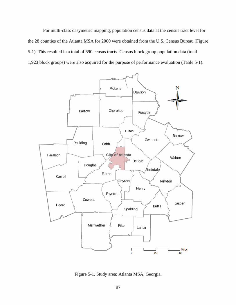
97

For multi-class dasymetric mapping, population census data at the census tract level for

the 28 counties of the Atlanta MSA for 2000 were obtained from the U.S. Census Bureau (Figure

5-1). This resulted in a total of 690 census tracts. Census block group population data (total

1,923 block groups) were also acquired for the purpose of performance evaluation (Table 5-1).

City of Atlanta

Fulton

Meriwether

FultonCarroll

Cobb

Bartow

CowetaJasper

Henry

Pike

Heard

Gwinnett

Walton

Cherokee

DeKalb

Paulding

Butts

Newton

Forsyth

Haralson

Pickens

Lamar

Fayette

Dawson

Douglas

Spalding

Barrow

Clayton

Rockdale

Figure 5-1. Study area: Atlanta MSA, Georgia.

98

Table 5-1. Census hierarchy in Atlanta MSA

Level # Zones

County 28 Census tract 690 Census block group 1,923

A land cover map for the 28 counties of Atlanta MSA (Figure 5-2) was extracted from

the National Land Cover Dataset (NLCD) 2001 downloaded from the Multi-Resolution Land

Characteristics Consortium (MRLC; http://www.mrlc.gov/). The MRLC is a group of federal

agencies that joined together in 1993 to purchase Landsat 5 imagery for the conterminous U.S.

and to develop a land cover dataset called the National Land Cover Dataset (NLCD 1992). In

1999, a second-generation MRLC consortium was formed to purchase three dates of Landsat 7

imagery for the entire United States (MRLC 2001) and to coordinate the production of a

comprehensive land cover database for the nation called the National Land Cover Database

(NLCD 2001). The NLCD 2001, derived from Landsat satellite images, provides pre-classified

information on land cover category types, including urban land covers, at 30 m resolution for the

entire United States. The NLCD data are free, seamless, and downloadable from

http://seamless.usgs.gov/website/seamless/viewer.php. The overall database philosophy and

classification methodology were presented by Homer et al (2004).

99

Figure 5-2. National Land Cover Dataset (NLCD) 2001

100

The NLCD program has many advantages for dasymetric mapping of population

distribution. Given that the difficulty of land cover classification is one of the main reasons why

the dasymetric mapping method is not being widely accepted for population distribution

mapping in spite of its better performance over simple areal weighting interpolation as briefly

discussed above, a freely available land cover dataset like NLCD provides a good alternative to

obtain land cover dataset for dasymetric mapping. Also since the first NLCD was distributed in

1992, it was updated in 2001. Another update is being undertaken by MRLC for 2006 as a

national land cover monitoring program. Regular updates of the national land cover maps would

also provide an opportunity for accurate population distribution mapping in timely manner.

To implement dasymetric mapping method with the NLCD dataset, the issue of land

cover classification scheme needs to be addressed properly. Whereas its predecessor, NLCD

1992, uses a classification scheme differentiating urban land cover into three classes that

explicitly describe land use (Low intensity residential, high intensity residential, and commercial

/ industrial / transportation), NLCD 2001 (and 2006 update) does not explicitly differentiate

urban land uses. Conceptually, dasymetric mapping utilizes land use information from the

ancillary data to redistribute population counts to residential area. The delineation of residential

land use therefore has a huge impact on the accuracy of the method. However, land cover may

not be directly associated with land use even though both terms are often used together.

Anticipated to be a more objective and consistent dataset that can accommodate a variety

of potential users and producers, the NLCD 2001 does not explicitly represent different urban

land uses. The NLCD 2001 does divide ‘developed’ areas into four land cover classes according

to their impervious surface fraction as summarized in Table 5-2 (Homer et al. 2004).

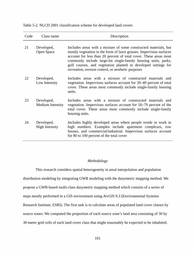
101

Table 5-2. NLCD 2001 classification scheme for developed land covers

Code Class name Description

21 Developed,

Open Space Includes areas with a mixture of some constructed materials, but mostly vegetation in the form of lawn grasses. Impervious surfaces account for less than 20 percent of total cover. These areas most commonly include large-lot single-family housing units, parks, golf courses, and vegetation planted in developed settings for recreation, erosion control, or aesthetic purposes

22 Developed, Low Intensity

Includes areas with a mixture of constructed materials and vegetation. Impervious surfaces account for 20–49 percent of total cover. These areas most commonly include single-family housing units.

23

Developed, Medium Intensity

Includes areas with a mixture of constructed materials and vegetation. Impervious surfaces account for 50–79 percent of the total cover. These areas most commonly include single-family housing units.

24

Developed, High Intensity

Includes highly developed areas where people reside or work in high numbers. Examples include apartment complexes, row houses, and commercial/industrial. Impervious surfaces account for 80 to 100 percent of the total cover

Methodology

This research considers spatial heterogeneity in areal interpolation and population

distribution modeling by integrating GWR modeling with the dasymetric mapping method. We

propose a GWR-based multi-class dasymetric mapping method which consists of a series of

steps mostly performed in a GIS environment using ArcGIS 9.3 (Environmental Systems

Research Institute, ESRI). The first task is to calculate areas of populated land cover classes by

source zones. We computed the proportion of each source zone’s land area consisting of 30 by

30-meter grid cells of each land cover class that might reasonably be expected to be inhabited.

102

The four ‘developed’ land cover classes of the NLCD 2001 classification scheme are assumed to

be inhabited and other non-residential land cover classes are omitted from the interpolation

entirely: thus, none of the population is assigned to these areas. The source zones’ population

counts are then regressed on the areas of populated land cover classes using the OLS regression

model and GWR model. Once the weights have been initially determined by both models, they

are applied to the NLCD data layer to generate a population density surface map. To evaluate the

performance of the proposed method, we will conduct a comparative investigation to determine

the accuracies of different areal interpolation methods: areal weighting interpolation, binary

dasymetric mapping, and multi-class dasymetric methods with a global regression model and

with GWR model. Each method is calibrated with 2000 census tract population and the NLCD

2001 data, and census block group population is estimated by each method. These estimates are

compared to the actual block group census data to evaluate the performance of the proposed

method.

The simplest scheme to implement dasymetric mapping with the NLCD 2001 data

would be the binary method in which NLCD 2001 map is reclassified to a binary map of

‘populated’ and ‘empty’ pixels and census population is redistributed to only those populated

pixels. Pixels of the low intensity developed and medium intensity developed classes are to be

reclassified as ‘populated’ pixels in the binary method, as those classes are described as related to

residential land use exclusively. Descriptions for the other two developed land cover classes

(Open space and High intensity), however, are rather generalized implying that those pixels

could be interpreted as different land use types according to where they belong. The binary

dasymetric method is conceptually simple and easy to implement. However, population

distribution in urban areas is thought to be more complex than that modeled by the simple

103

populated/empty distinction. It seems likely that population densities would vary by land cover

classes in reality. Various housing types ranging from large-lot single family housing to

apartment complexes would have completely different residential density values. Moreover it is

highly probable that pixels with a same land cover class might have different land uses according

to where they belong. For example, in an urban center, high intensity developed areas could be

interpreted as various urban land uses ranging from multi-family housing complexes to

commercial buildings, whereas, in a suburban area where multi-family housing unit is rare, those

areas are mostly not residential. The relationship between land cover class and population

density might vary spatially as well. The problem of spatial heterogeneity, which the OLS model

cannot address, makes the implementation of multi-class dasymetric method even harder.

Model calibration

Global regression model

Regression model calibration to determine density parameters for land cover classes

consists of step-by-step refinements to include relevant variables and exclude irrelevant ones.

Langford et al (1991) stated that there is a conflict between a desire to maximize the fit obtained,

by inclusion of as many statistically significant terms as possible, and simple logic which

suggests that the correct form of any fitted model should be a linear weighted sum of only those

land cover types that people actually live in, without any intercept term. With this in mind, we

calibrate the global OLS regression model for dasymetric mapping by a repetitive procedure

summarized in Table 5-3.

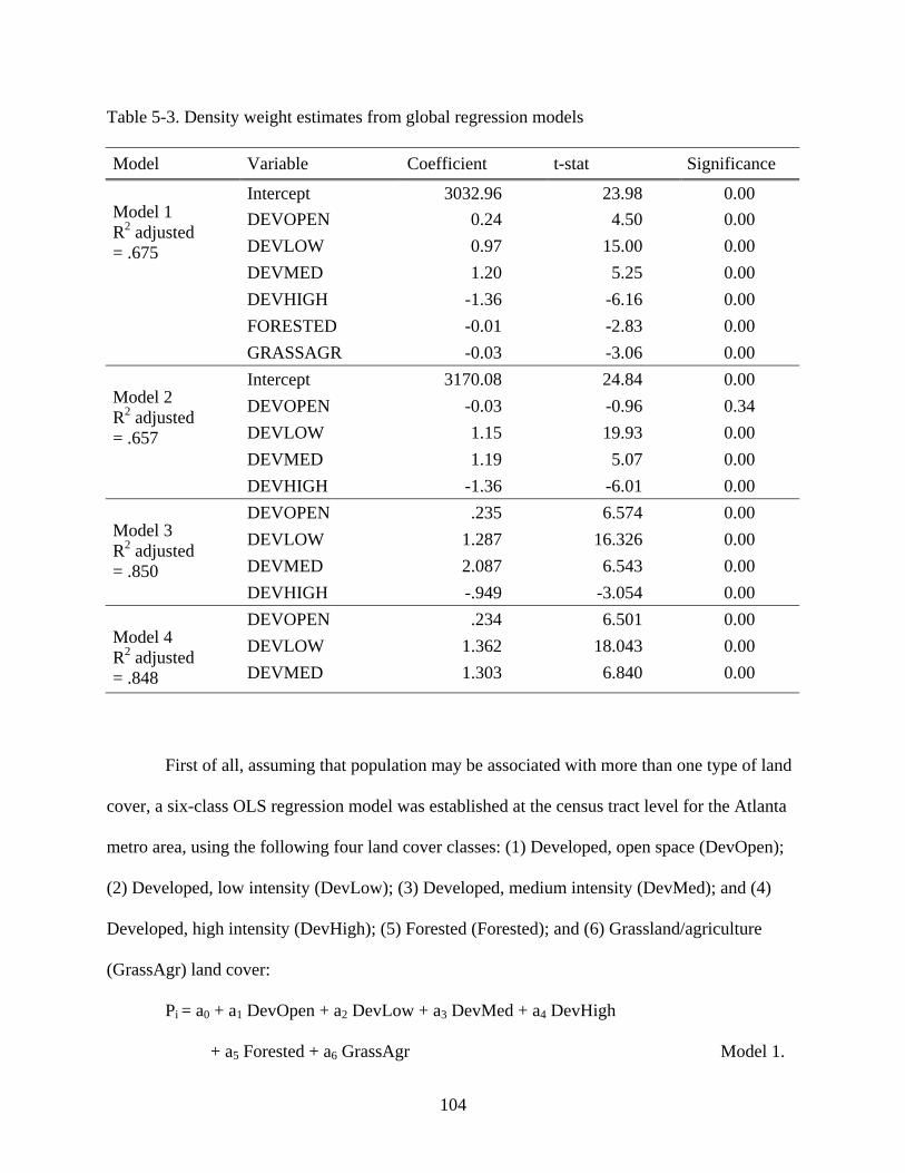
104

Table 5-3. Density weight estimates from global regression models

Model Variable Coefficient t-stat Significance Model 1 R2 adjusted = .675

Intercept 3032.96 23.98 0.00 DEVOPEN 0.24 4.50 0.00 DEVLOW 0.97 15.00 0.00 DEVMED 1.20 5.25 0.00 DEVHIGH -1.36 -6.16 0.00 FORESTED -0.01 -2.83 0.00 GRASSAGR -0.03 -3.06 0.00

Model 2 R2 adjusted = .657

Intercept 3170.08 24.84 0.00 DEVOPEN -0.03 -0.96 0.34 DEVLOW 1.15 19.93 0.00 DEVMED 1.19 5.07 0.00 DEVHIGH -1.36 -6.01 0.00


DEVOPEN .235 6.574 0.00 DEVLOW 1.287 16.326 0.00 DEVMED 2.087 6.543 0.00 DEVHIGH -.949 -3.054 0.00


DEVOPEN .234 6.501 0.00 DEVLOW 1.362 18.043 0.00 DEVMED 1.303 6.840 0.00

First of all, assuming that population may be associated with more than one type of land

cover, a six-class OLS regression model was established at the census tract level for the Atlanta

metro area, using the following four land cover classes: (1) Developed, open space (DevOpen);

(2) Developed, low intensity (DevLow); (3) Developed, medium intensity (DevMed); and (4)

Developed, high intensity (DevHigh); (5) Forested (Forested); and (6) Grassland/agriculture

(GrassAgr) land cover:

Pi = a0 + a1 DevOpen + a2 DevLow + a3 DevMed + a4 DevHigh

+ a5 Forested + a6 GrassAgr Model 1.

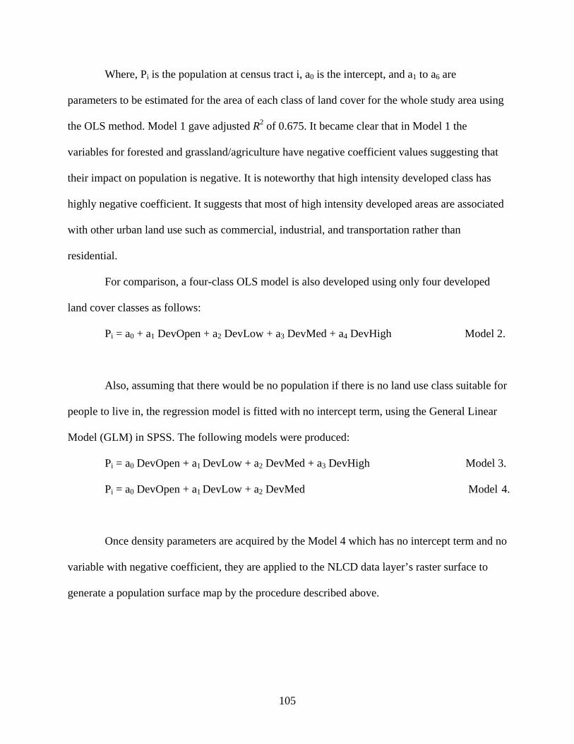
105

Where, Pi is the population at census tract i, a0 is the intercept, and a1 to a6 are

parameters to be estimated for the area of each class of land cover for the whole study area using

the OLS method. Model 1 gave adjusted R2 of 0.675. It became clear that in Model 1 the

variables for forested and grassland/agriculture have negative coefficient values suggesting that

their impact on population is negative. It is noteworthy that high intensity developed class has

highly negative coefficient. It suggests that most of high intensity developed areas are associated

with other urban land use such as commercial, industrial, and transportation rather than

residential.

For comparison, a four-class OLS model is also developed using only four developed

land cover classes as follows:

Pi = a0 + a1 DevOpen + a2 DevLow + a3 DevMed + a4 DevHigh Model 2.

Also, assuming that there would be no population if there is no land use class suitable for

people to live in, the regression model is fitted with no intercept term, using the General Linear

Model (GLM) in SPSS. The following models were produced:

Pi = a0 DevOpen + a1 DevLow + a2 DevMed + a3 DevHigh Model 3.

Pi = a0 DevOpen + a1 DevLow + a2 DevMed Model 4.

Once density parameters are acquired by the Model 4 which has no intercept term and no

variable with negative coefficient, they are applied to the NLCD data layer’s raster surface to

generate a population surface map by the procedure described above.

106

Geographically Weighted Regression model

The GWR model provides locally varying parameter estimates for regression models

where spatially varying relationships are hypothesized. The GWR software (version 3.0.16,

2003) produces unique parameter estimates for all observations by spatially weighting the

observations (i.e. census tract) according to their proximity to each other. Observations closer to

each other are given more weight than are observations further away. The weights are derived

through a distance-decay function to assign weights to data according to their proximity so that

near locations have more influence than further locations. To limit the number of data points

considered for each local parameter estimate, a spatial kernel is used at each observation. The

kernel can be either fixed, in which case the bandwidth of the kernel is also fixed, and thus

varying numbers of observations are weighted for the computation of each local parameter.

Because the census tracts in the Atlanta metro area have different sizes and are irregularly

distributed, an adaptive kernel is more appropriate. With an adaptive kernel, an equal number of

data observations are weighted and used for local parameter estimation. In addition to local

parameter estimates, the GWR program also provides local goodness-of-fit measures and local

residuals. The GWR model is compared with the global regression model (Model 2) of the same

dependent and independent variables. The Akaike Information Criteria (AIC) values and the

adjusted R2 are compared against each other.

For this analysis, a geographically weighted Gaussian regression is applied to the whole

study area at the census tract level using an adaptive kernel. The dependent variable is population

count, and the four developed land cover classes are used as independent variables as the third

OLS model: (1) Developed, open space (DevOpen); (2) Developed, low intensity (DevLow); (3)

Developed, medium intensity (DevMed); and (4) Developed, high intensity (DevHigh). We did

107

not exclude the high intensity developed land cover in the GWR model assuming that it might

have different density coefficients according to its location, even though it shows negative

coefficients in all the OLS regression models.

The results from the model show that the Akaike Information Criterion for the GWR

model (12,227) is smaller than that for the global OLS model (12,436), which indicates that the

GWR model is better than the global OLS model. Also, the adjusted R2 value of the local GWR

model is 0.787, a great improvement from the 0.657 of the global OLS model (Model 2). A test

for spatial variability of the five parameters in the GWR model using the Monte Carlo

significance test reveals that only high intensity developed land cover (DevHigh) is not

significant in spatial heterogeneity, while it is highly significant (at 0.1% level) for the other

three developed land cover classes (Open, Low, and Medium), which means those classes show

more spatial heterogeneity in the relationship with population density. Table 5-4 shows a sample

of input data, estimated parameters, local R2, and residual of census tracts for the four-class

GWR model.

108

Table 5-4. Parameter estimation using the Four-class GWR model (sampled)

Obs Cond Local R2 Pred Interc C1

DevOpenC2 DevLow

C3 DevMed

C4 DevHigh Residual

5118 10.42 0.71 6130.20 1742.20 0.25 0.89 0.83 -1.02 -1012.20 3161 10.21 0.74 5486.39 1643.88 0.27 1.10 -1.16 -0.38 -2325.39 5517 9.91 0.74 5938.06 1890.12 0.26 1.11 -1.24 -0.44 -421.06 6008 9.83 0.74 5892.76 2082.89 0.25 1.08 -0.90 -0.83 115.24 8498 9.49 0.76 7563.24 2728.00 0.24 0.94 0.87 -2.43 934.76 10595 9.39 0.86 9718.03 2878.50 0.27 1.09 -0.48 -1.47 876.97 10930 10.72 0.82 8644.43 2204.64 0.30 1.25 -2.35 0.88 2285.57 5212 10.01 0.75 5697.75 1840.76 0.28 1.18 -1.68 0.03 -485.75 5648 10.54 0.75 7005.03 1706.99 0.26 1.37 -2.28 0.83 -1357.03 10130 12.23 0.71 11455.30 1753.54 0.16 0.70 2.92 -1.59 -1325.30 4970 11.70 0.70 5822.27 1971.20 0.19 0.67 3.07 -1.95 -852.27 6098 10.60 0.71 7107.71 1490.47 0.21 0.72 2.58 -1.35 -1009.71 4641 10.34 0.71 5981.30 1455.97 0.22 0.74 2.36 -1.28 -1340.30 7071 10.49 0.72 8252.18 1368.84 0.21 0.72 2.48 -1.18 -1181.18 5632 10.47 0.72 7260.55 1122.09 0.24 0.78 1.88 -0.83 -1628.55 7602 10.46 0.71 9121.19 1500.77 0.24 0.76 2.05 -1.25 -1519.19 8667 13.28 0.75 7690.76 2152.08 0.02 1.46 1.20 -3.56 976.24 7756 13.11 0.77 8278.59 1810.84 0.03 1.61 0.70 -3.36 -522.59 4085 12.74 0.76 4749.18 1719.70 0.03 1.71 0.52 -3.34 -664.18 11846 12.83 0.75 13500.60 2126.64 0.01 1.59 0.91 -3.40 -1654.60 5211 12.52 0.76 7088.33 1915.96 0.01 1.69 0.62 -3.22 -1877.33 7604 12.32 0.77 7061.52 1800.51 -0.01 1.79 0.40 -2.91 542.48 5747 12.69 0.75 6118.50 2390.41 -0.04 1.59 0.95 -3.09 -371.50 3171 12.74 0.80 4947.80 2568.27 -0.19 1.89 -0.04 -1.58 -1776.80 2911 12.77 0.80 4979.51 2359.66 -0.17 1.94 -0.21 -1.44 -2068.51 4423 12.45 0.78 7337.75 1817.65 -0.05 1.89 0.03 -2.19 -2914.75 8389 12.03 0.77 7363.76 1566.25 0.01 1.86 0.15 -2.81 1025.24 6209 11.65 0.79 6611.16 1054.88 0.04 1.98 -0.22 -2.73 -402.16 3386 8.50 0.85 3276.81 590.12 0.01 2.01 -2.39 1.43 109.19 8607 8.73 0.83 9955.76 838.46 -0.03 1.98 -2.36 1.32 -1348.76 7374 9.24 0.78 7540.40 1184.71 -0.07 1.92 -2.26 1.08 -166.40 5336 10.14 0.75 5913.27 1792.95 -0.13 1.76 -2.09 1.17 -577.27 3649 10.44 0.75 4230.95 1931.79 -0.14 1.70 -1.99 1.26 -581.95 7114 10.48 0.78 5345.50 1794.23 -0.12 1.75 -2.17 1.48 1768.50 3547 10.52 0.78 3466.84 1784.49 -0.12 1.75 -2.22 1.56 80.16 4680 10.07 0.78 4339.32 1674.59 -0.11 1.80 -2.25 1.37 340.68 6221 10.56 0.82 5979.90 1593.52 -0.08 1.78 -2.29 1.64 241.10 7021 9.83 0.80 6975.67 1482.27 -0.09 1.85 -2.29 1.37 45.33 3903 11.25 0.87 4331.28 1410.12 -0.03 1.73 -1.85 1.26 -428.28 3494 11.27 0.81 3723.40 1911.23 -0.12 1.68 -2.00 1.62 -229.40

109

The performance of the GWR model can be accessed by comparing the accuracy of

population estimation with that of OLS model. The population estimation based on the Atlanta

census tracts produced from the local four-class GWR model is more accurate (a mean relative

error of –10.78% and a RMSE of ±1497.42) than that produced from the global OLS model (-

22.33% and ±2145.23). The GWR model produced local parameter estimates for each of the

variables in the model for each census tract, which can be mapped. These parameter estimates

show the strength of the relationship of each variable (land cover) to population by location.

Thus, for most land cover classes, there is high spatial heterogeneity and the local parameter

estimates change sign over space

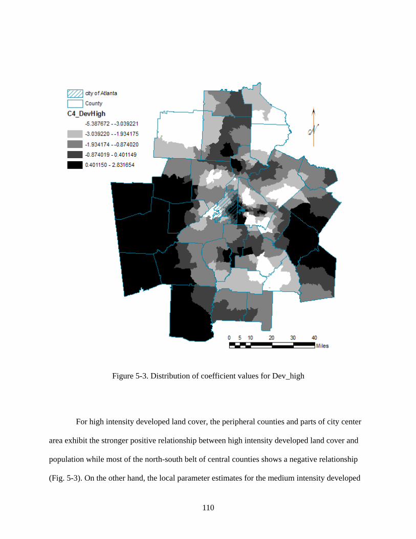
110

Figure 5-3. Distribution of coefficient values for Dev_high

For high intensity developed land cover, the peripheral counties and parts of city center

area exhibit the stronger positive relationship between high intensity developed land cover and

population while most of the north-south belt of central counties shows a negative relationship

(Fig. 5-3). On the other hand, the local parameter estimates for the medium intensity developed

111

land cover variable show high values (stronger relationship) in the core and rapidly growing

suburban counties (Gwinnett, Forsyth, and Barrow), gradually trending down to low values

(weaker relationship) in the periphery (Fig. 5-4). This displays a stronger core-periphery

influence for Dev_med than that for the Dev_high.

Figure 5-4. Distribution of coefficient values for Dev_med

112

Figure 5-5. Distribution of coefficient values for Dev_low

As for the local parameter estimates for the low intensity developed land cover variable,

which remain positive almost throughout (Figure 5-5), the spatial distribution of the parameter

estimates shows a inverse pattern from that of Dev_med. High population density areas such as

the city core and major suburban residential area show weaker relationship between the area of

Dev_low and population count while peripheral areas show stronger relationship. Finally, the

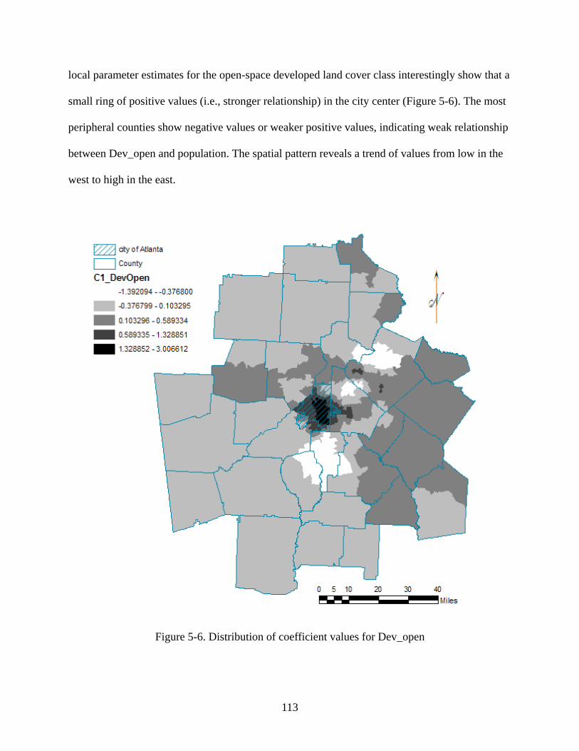
113

local parameter estimates for the open-space developed land cover class interestingly show that a

small ring of positive values (i.e., stronger relationship) in the city center (Figure 5-6). The most

peripheral counties show negative values or weaker positive values, indicating weak relationship

between Dev_open and population. The spatial pattern reveals a trend of values from low in the

west to high in the east.

Figure 5-6. Distribution of coefficient values for Dev_open

114

Figure 5-7. Local R2 values

Taking the four-class model as a whole, the map of pseudo local R2 values shows the

strongest relationship between population and land cover in some clusters south of the central

city and most of peripheral areas. The weakest relationship is found in high density urban areas

of Fulton, Cobb, DeKalb, and Clayton County around the central city (less than 0.5) (Figure 5-7).

This suggests that each of these parts has more complicated residential density pattern, which is

difficult to be modeled by only land cover areas.

115

Overall, the results of GWR model and the spatial pattern of parameter estimates for

each land cover class show that spatial heterogeneity problem is evident in the relationship

between land cover classes and population counts.

Implementation and performance evaluation

Once the weights (parameter estimates) have been initially determined by the GWR

modeling, they are applied to the NLCD data layer to generate population density surface map. It

is important to recall, however, because the model does not accounts for all the variation in the

source zone population, the density weights need to be locally scaled by the ratio of their

respective source zone’s observed population to its fitted population to account for the

proportion of source zone population not predicted in the model, thus preserving the

pycnophylactic property (Flowerdew and Green 1989; Flowerdew and Green 1992; Yuan et al.

1997) as in equation 7. For OLS regression model, where intercept and negative coefficient are

excluded assuming no population for no residential area, the grid cells forming the raw estimated

population surface were multiplied by the ratio of their respective source tracts’ observed

populations to the source tract’s fitted population computed by summing the raw estimates

across the source tract’s grid cells.

On the contrary, the GWR model does not exclude intercept term and negative parameter

estimates provided that land cover class does not directly associated with residential land use.

Hence, we assume that a certain land cover may have a negative effect on population density and

intercept term could be a part of variance not explained by the four land cover class variables.

Assuming that the intercept term and error term in the GWR model refer to the variance that is

not explained by the four developed land cover classes, those values are evenly redistributed to

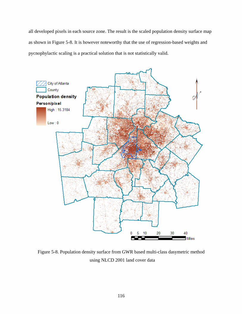
116

all developed pixels in each source zone. The result is the scaled population density surface map

as shown in Figure 5-8. It is however noteworthy that the use of regression-based weights and

pycnophylactic scaling is a practical solution that is not statistically valid.

Figure 5-8. Population density surface from GWR based multi-class dasymetric method

using NLCD 2001 land cover data

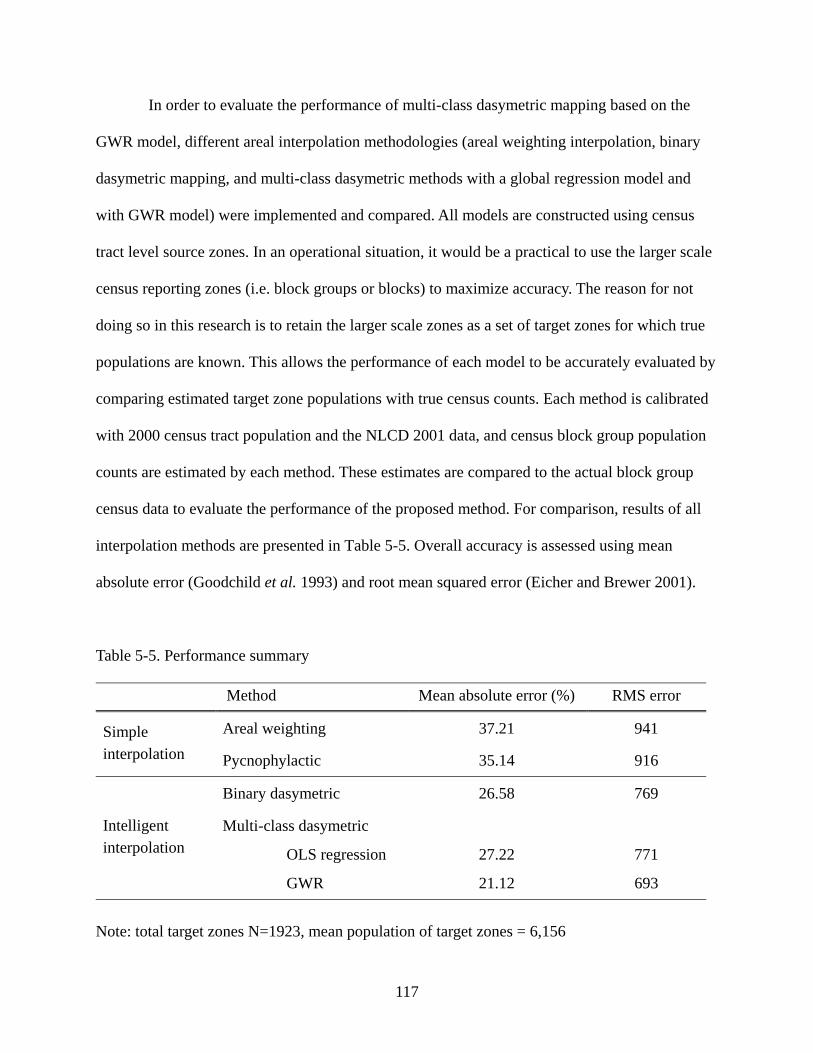
117

In order to evaluate the performance of multi-class dasymetric mapping based on the

GWR model, different areal interpolation methodologies (areal weighting interpolation, binary

dasymetric mapping, and multi-class dasymetric methods with a global regression model and

with GWR model) were implemented and compared. All models are constructed using census

tract level source zones. In an operational situation, it would be a practical to use the larger scale

census reporting zones (i.e. block groups or blocks) to maximize accuracy. The reason for not

doing so in this research is to retain the larger scale zones as a set of target zones for which true

populations are known. This allows the performance of each model to be accurately evaluated by

comparing estimated target zone populations with true census counts. Each method is calibrated

with 2000 census tract population and the NLCD 2001 data, and census block group population

counts are estimated by each method. These estimates are compared to the actual block group

census data to evaluate the performance of the proposed method. For comparison, results of all

interpolation methods are presented in Table 5-5. Overall accuracy is assessed using mean

absolute error (Goodchild et al. 1993) and root mean squared error (Eicher and Brewer 2001).

Table 5-5. Performance summary

Method Mean absolute error (%) RMS error

Simple interpolation

Areal weighting 37.21 941

Pycnophylactic 35.14 916

Intelligent interpolation

Binary dasymetric 26.58 769

Multi-class dasymetric

OLS regression 27.22 771

GWR 21.12 693 Note: total target zones N=1923, mean population of target zones = 6,156

118

Including the GWR based multi-class dasymetric method proposed in this study, a total

five interpolation methods are implemented. The simple areal weighting interpolation and

pycnophylactic interpolation provides benchmarks against which the intelligent methods can be

compared. All intelligent interpolation methods outperform areal weighting interpolation and

pycnophylactic interpolation. The overall accuracy of binary dasymetric method is better than

that of the multi-class dasymetric method based on OLS regression model. This result is

consistent with the previous finding of Fisher and Langford (1995): a globally fitted regression

model gives poorer accuracy than the locally fitted dasymetric method. It is interesting that OLS

regression based multi-class dasymetric method shows poorer performance even after the

parameter estimates of the regression model are locally fitted by pycnophylactic scaling. It seems

that, using a global regression model, benefits of employing multiple land cover classes rather

than one land cover class are not realized. It might be because of the ambiguity in the

relationship between land cover and land use as discussed above. Also, population density

parameters determined by global regression model are fixed throughout the study area and so

cannot account for spatial heterogeneity. Although the dasymetric approach inherently allows

local fitting by pycnophylactic scaling in nature, it is evident that further flexibility in parameter

specification might yield additional benefits.

Unlike OLS regression based method which excludes intercept and negative coefficient

assuming no population for no residential area, GWR based dasymetric mapping allows any land

cover class to have a negative density parameter as well as a positive parameter. Therefore, each

land cover class may have varying density parameters area by area as shown in Figures 5-3 to

Figure 5-6, and Table 5-4. Those figures show that a certain land cover class may have a

negative effect on the population density in some regions, while positively correlated with

119

population density in most areas, and vice versa. For instance, high intensity developed land

cover has positive density parameters in the eastern and western parts rural area while most of

study area have negative parameters. On the other hand, medium intensity developed land cover

shows negative parameters for those rural areas while positive parameters are prevalent in most

areas.

GWR based dasymetric allows the spatial heterogeneity of land cover – population

density correlation to be accounted. The intercept term is evenly distributed to all pixels in the

source zone to ensure any pixel not to have negative population density value. Accuracy

measures in Table 5-5 prove that multi-class dasymetric mapping can be improved by GWR

based parameter estimation to account for spatial heterogeneity.

120

CONCLUSIONS

This paper examined the benefits of the geographical weighted regression (GWR) for

dasymetric density parameter estimation in the context of population distribution modeling. For

ancillary dataset used in the dasymetric method, we used the pre-classified NLCD 2001 land

cover dataset that does not require digital image processing and classification. The performance

of the GWR based multi-class dasymetric mapping method was examined by a comparative

accuracy assessment with four other areal interpolation methods for population distribution

modeling. All intelligent interpolation methods outperformed the areal weighting interpolation

and the pycnophylactic interpolation, both of which do not utilized ancillary information. OLS

based multi-class dasymetric method did not show better performance than the binary dasymetric

method. GWR based multi-class dasymetric method was found to provide the most accurate

result. The degree to which this technique was found to be superior is attributed to the fact that

spatial heterogeneity was accounted for in the process of determining density parameters for land

cover classes.

Overall, this research showed that the performance of dasymetric mapping method can

be improved by integrating the geographically weighted regression model to determine weight

parameters of land cover classes on population density, which is a crucial part of the estimation

process. It is also noteworthy that the proposed method performed well with the NLCD 2001, a

publically available high quality national land cover dataset. We anticipate these data and

methods would fulfill the need for accurate population distribution data without the effort to

classify remotely sensed images.

121

REFERENCE





———. 1995. Linkage of the 1981 and 1991 UK Censuses using surface modelling concepts.




Dixon, O. M. 1972. Method and progress in choropleth mapping of population density. The

Cartographic Journal 9:19-29.




Dobson, J. E., E. A. Bright, R. Coleman, R. G. Durfee, and B. A. Worley. 2000. LandScan: A

global population database for estimating population at risk. Photogrammetric

Engineering & Remote Sensing 66 (7):849-857.







122




———. 1992a. Developments in areal interpolation methods and GIS. Annals of Regional

Science 26 (1):67.

———. 1992b. Statistical methods for inference between incompatible zonal systems. In The

Accuracy of Spatial Databases, eds. M. F. Goodchild and S. Gopal, 239-247. London:

Taylor and Francis.

———. 1994. Areal interpolation and types of data. In Spatial Analysis and GIS, eds. A. S.

Fotheringham and P. Rogerson. London: Talyor & Francis.

Fotheringham, A. S., C. Brunsdon, and M. Charlton. 2002. Geographically weighted regression :

the analysis of spatially varying relationships. Chichester: Wiley.

Fotheringham, A. S., and D. W. S. Wong. 1991. The modifiable areal unit proble in multivariate

statistical analysis. Environment & Planning A 23:1025-1044.

Garb, J. L., R. G. Cromley, and R. B. Wait. 2007. Estimating Populations at Risk for Disaster

Preparedness and Response. Journal of Homeland Security and Emergency Management

4 (1):1-17.



Goodchild, M. F., and N. S. Lam. 1980. Areal Interpolation: A variant of the traditional spatial

problem. Geo-Processing 1:297-312.

123

Gregory, I. N. 2002. The accuracy of areal interpolation techniques: standardising 19th and 20th

century census data to allow long-term comparisons. Computers, Environment and Urban

Systems 26 (4):293-314.

Hay, S. I., A. M. Noor, A. Nelson, and A. J. Tatem. 2005. The accuracy of human population

maps for public health application. Tropical Medicine and International Health 10

(20):1073-1086.



(2):103-121.

Homer, C., C. Huang, L. Yang, B. Wylie, and M. Coan. 2004. Development of a 2001 National

Landcover Database for the United States. Photogrammetric Engineering & Remote

Sensing 70 (7):829-840.

Huang, Y., and Y. Leung. 2002. Analysing Regional Industrialization in Jiangsu Province Using

Geographically Weighted Regression. Journal of Geographical Systems 4:233-249.


(2):129-149.

Langford, M. 2003. Refining methods for dasymetric mapping. In Remotely Sensed Cities, ed. V.


———. 2006. Obtaining population estimates in non-census reporting zones: An evaluation of

the 3-class dasymetric method. Computers, Environment and Urban Systems 30 (2):161-

180.



124

Langford, M., and G. Higgs. 2006. Measuring Potential Access to Primary Healthcare Services:

The Influence of Alternative Spatial Representations of Population. Professional

Geographer 58 (3):294-306.







Lo, C. 2008. Population Estimation Using Geographically Weighted Regression. GIScience &

Remote Sensing 45 (2):131-148.

Lo, C. P. 1986. Applied Remote Sensing: Harlow: Longman.

Luo, J. 2005. Analyzing urban spatial structure with GIS population surface model. Paper read at

UCGIS summer assembly, at Jackson hall, Wyoming.

Martin, D. 1989. Mapping Population Data from Zone Centroid Locations. Transactions of the

Institute of British Geographers 14 (1):90-97.

———. 1996. An assessment of surface and zonal models of population. International Journal

of Geographical Information Science 10 (8):973-989.

Martin, D., N. J. Tate, and M. Langford. 2000. Refining Population Surface Models:

Experiments with Northern Ireland Census Data. Transactions in GIS 4 (4):343.

McCleary, G. F., Jr. 1984. Cartography, geography and the dasymetric method. Paper read at 12th

conference of international cartographic association, at Perth, Australia.

125



Mennis, J., and T. Hultgren. 2006. Intelligent Dasymetric Mapping and Its Application to Areal

Interpolation. Cartography and Geographic Information Science 33 (3):179-194.

Moon, Z. K., and F. L. Farmer. 2001. Population Density Surface: A New Approch to an Old

Problem. Society and Natural Resources 14:39-49.



Okabe, A., and Y. Sadahiro. 1997. Variation in count data transferred from a set of irregular

zones to a set of regular zones through the point-in-polygon method. International

Journal of Geographical Information Science 11:93-106.

Openshaw, S., and L. Rao. 1995. Algorithms for reengineering 1991 Census geography.


Rase, W. 2001. Volume-preserving interpolation of a smooth surface from polygon-related data.

Journal of Geographical Systems 3 (2):199.

Reibel, M., and A. Agrawal. 2007. Areal Interpolation of Population Counts Using Pre-classified

Land Cover Data. Population Research and Policy Review 26:619-633.



Sadahiro, Y. 2000. Accuracy of Areal Interpolation: A Comparison of Alternative Methods.

Journal of Geographical Systems 1 (4):323-346.

126

Sleeter, R. 2004. Dasymetric mapping techniques for the San Francisco bay region, California.

Paper read at Urban and Regional Information Systems Association Annual Conference,

November 7–10, 2004., at Reno, NV.

Sutton, P. 1997. Modeling population density with night-time satellite imagery and GIS.

Computers, Environment and Urban Systems 21 (3-4):227-244.

Sutton, P., D. Roberts, C. Elvidge, and K. Baugh. 2001. Census from Heaven: an estimate of the

global human population using night-time satellite imagery. International Journal of

Remote Sensing 22 (16):3061-3076.

Tobler, W. 1970. A computer movie simulating urban growth in the Detroit region. Economic

Geography 46 (2):234-240.

———. 1979. Smooth pycnophylactic interpolation for geographic regions. Journal of the




Wu, S., X. Qiu, and L. Wang. 2005. Population estimation methods in GIS and remote sensing: A

review. GIScience & Remote Sensing 42 (1):80-96.

Xie, Y. 1996. The Overlaid Network Algorithms for Areal Interpolation Problem. Computers,

Environment and Urban Systems 19:287-306.

Yang, X., and C. P. Lo. 2002. Using a Time Series of Satellite Imagery to Detect Land Use and

Land Cover Changes in the Atlanta, Georgia Metropolitan Area. International Journal of

Remote Sensing 23 (9):1775-1798.

127



(3-4):245-258.

128

CHAPTER 6

CONCLUSIONS AND FUTURE RESEARCH

CONCLUSIONS

Demographic data are mostly aggregated into areal units designed to be homogeneous

with respect to population characteristics, economic status, and living conditions. Intelligent

interpolation and dasymetric mapping methods are techniques that utilize ancillary data (such as

that obtained from remotely sensed images) to redistribute population data from arbitrarily

delineated enumeration districts into units that are, internally, more homogenous in order to

better represent the actual underlying statistical surface. Due to the increasing availability of

remotely sensed data, it becomes pressing to develop an efficient methodology for

implementation of high-accuracy dasymetric mapping methods based on raster-based land cover

datasets.

This research has addressed several issues related to the accuracy and efficiency of

dasymetric mapping methods for high resolution population distribution surface modeling using

a pre-classified raster land cover dataset. In Chapter 2, I compared the performances of five

regression-based population estimation models using U.S. Census Bureau 1990 census block

group population count data and areas of the NLCD 1992 land cover classes. High and low

intensity residential land cover classes are found to have highly positive correlation with

population counts, while addition of other independent variables (other land cover classes) and

129

variable manipulation (logarithmic transformation) did not improve the performance. Once land

cover classes that have significant positive relationships with population density are determined

as in Chapter 2, the population density value of each land cover is obtained deterministically for

each source zone. In the binary dasymetric method, it is simply calculated by dividing population

count of the source zone by the number of residential pixels in the source zone. Even with multi-

class dasymetric methods in Chapter 3, a population density parameter for each land cover class

is assigned in similar ways, which could be arbitrary in the case of the three-class method or

deterministic as in the limiting variable method. Consequently, the performance superiority of

dasymetric methods with multiple land cover classes over that of the binary dasymetric method

is inconclusive in spite of their methodological complexity.

Given that binary dasymetric mapping has shown to be a robust and effective method for

enhancing areal interpolation and population mapping as reported in Chapter 3 and other

research (Fisher and Langford 1995; 1996), what lies in the future in terms of methodological

development? The aim must be to enhance its performance further by overcoming its

shortcomings. With the binary dasymetric method, any resultant error can arise from one of two

sources. The first is through the incorrect identification of residential areas in the satellite image.

If areas that are not residential are classified as residential, it will lower the mean population

density of all residential areas contained within the source unit, as well as it will distribute

population into places where it should not be present. So, higher classification accuracy is clearly

a desirable goal. The second source of errors is in the calibration of the dasymetric densities. In a

binary dasymetric map, the assumption is made that all residential areas in any specific source

unit will have the same population density. As reported in Chapter 3, this simple model has been

shown to be effective at enhancing the accuracy of areal interpolation when compared with a

130

choropleth or uniform density model. Despite this it still seems logical to assume that, in most

situations, there is likely to be some degree of variation in housing type, occupancy and thus

population density, within the boundaries of the source units. The differentiation of more than

one class of occupied land cover, each with an associated population density, is therefore another

area of potential development. The binary dasymetric method also suffers several methodological

and cartographical shortcomings. It assumes population densities are uniform among pixels of

the same land use land cover type within each source unit. As a result, abrupt changes of

population density can be found at borders of source zones and those between different land use

land cover. Therefore, the contrast of population density between two adjacent pixels with

different land use land cover classes is mistakenly exaggerated. Two adjacent residential pixels

may have much different population density values if those pixels fall into different source units

because the binary dasymetric method does not account for the neighborhood effect.

It seems logical, then, that there are three directions in which the dasymetric method can

be further advanced. First, we can refine the method of binary dasymetric method to account for

the neighborhood effect so that population densities of residential pixels are adjusted by those of

adjacent residential areas. In Chapter 4, we proposed a hybrid method integrating the

pycnophylactic interpolation with the binary dasymetric method. The subsequent pycnophylactic

interpolation creates a smoothed density surface by recalculating population density value of

each pixel with low-pass filtering process while preserving the original volume of each source

zone. The results show that the performance of the binary dasymetric method could be much

improved by a subsequent pycnophylactic smoothing. It proves that Tobler’s First Law of

geography is valid for population density distribution associated land cover.

131

Second, we can develop methods for the calibration of population densities associated

with multiple dasymetric classes. It is plausible to distinguish between several developed land

cover classes when classifying urban areas from satellite imagery, but the difficulty lies in

determining how appropriate density values should be assigned. It is even more difficult to

calibrate the relationship between land cover classes and population densities when the spatial

heterogeneity is present so the relationship varies place by place. In Chapter 5, we presented the

GWR based multi-class dasymetric mapping method to take into consideration the spatial

heterogeneity of underlying spatial relationships between population density and land cover

classes. Unlike the globally fitted regression model, GWR locally estimates the relationship of

each land cover class and the population density. Hence the proposed method allows each land

cover to have locally varied modeling parameters for the calculation of population density. The

benefits of accounting for spatial heterogeneity in population estimation are examined using the

pre-classified NLCD 2001 data. The performance of the proposed method is compared to four

other areal interpolation methods including areal weighting interpolation, pycnophylactic

interpolation, binary dasymetric method, and the globally fitted ordinary least squared (OLS)

based multi-class dasymetric method. By accounting for spatial heterogeneity, the GWR based

multi-class dasymetric method significantly outperforms all other methods.

Finally, the performance and applicability of the dasymetric mapping method can be

further improved by the accurate classification of the satellite image source and a choice of

appropriate spatial resolution of the ancillary dataset. The proposed methods in Chapter 3 and 4

utilize pre-classified, freely available land use land cover dataset with 30 meter spatial resolution.

It is worth noting that performances of the proposed methods are dependent on the accuracy and

the spatial resolution of those ancillary data, and are remained as avenues for future research.

132

FUTURE RESEARCH

Like any other areal interpolation method, the proposed methods of this dissertation have

limitations and problems also. These limitations are the starting point of future research.

Very high resolution ancillary data

It has long been argued that very high spatial resolution satellite imagery may not be

appropriate for the accurate identification of urban land cover, due to the complexity and

heterogeneity of the city landscape (Cushnie 1987; Woodcock and Srahler 1987; Hultgren 2005).

In the context of population mapping using ancillary data, the same relationship between spatial

resolution and accuracy ought to hold true. It has been suggested that regional population

estimation can be effectively performed at spatial resolution of 5 to 20 meter (Jensen and Cowen

1999). Others have speculated that as pixels are reduced to excessively small size in dasymetric

mapping, the overall error would increase (Eicher and Brewer 2001). However, this point of

view is generally founded on the assumption that a traditional per-pixel classification approach

has to be adopted. Very high spatial resolution imagery may result in better mapping of cities

provided alternative classification methods are adopted that can fully utilize texture

measurements, image segmentation, fuzzy classification, and object-based approaches (see Tso

and Mather 2001). Adaptations to the classification algorithms to make use of ancillary data

resources available in a GIS such as urban zonation and cadastral map, or even census-derived

statistics such as housing density measures (Mesev 1998), also offer an opportunity to enhance

urban image classification.

133

Error sources and error propagation

The proposed dasymetric methods use several sources of data and involve a few

analytical steps. The source data include the census data on the census tract and block group

level, and land use land cover data classified with the Landsat TM and ETM+ imagery. None of

the source data can be error free. The positional inaccuracy of census enumeration units, the

incorrect population counts, and the imperfect processing of the satellite imagery can all have an

impact on the performance of the proposed dasymetric methods. Further errors can also be

introduced and propagated during the intermediate stage of the method. To improve the

performance of the proposed methods, it is important to identify the critical data source and

method stage that have the most impact on the accuracy of the result. Monte Carlo simulation

can be run by making different scenarios with modified data source or method stage, and

examining the magnitude of changes in the method performance. The less the change, the less

impact that the data source or method stage has to the overall method. Anderson and Anderson

(1973) and Fisher and Langford (1995) both provided examples of evaluating the effect of the

land use land cover classification accuracy on population estimation. Those studies are valuable

for future research on error identification and propagation.

Nighttime vs. daytime population

In addition to the problem of spatial aggregation discussed throughout this dissertation,

the decennial population censuses conducted by the U.S. Census Bureau suffer from the

limitation of temporal scale. The U.S. Census uses de jure enumeration, which assigns persons

according to their usual place of residence. As a result, all the people recorded in a city are the

actual residents living in the city and exclude those who work but do not live in the city.

134

Moreover, the population is enumerated only at a specific moment in time. Daily movement of

the population is ignored. Because of the static nature of the population census, the U.S. Census

2000 indicated that there were only 55 people living in the large urban block that used to contain

the World Trade Center (Dobson et al. 2003). Since the World Trade Center attack of September

11, 2001, the Federal, State, and County governments are increasingly concerned about

homeland security, terrorism, and infectious diseases, among the many other threats to people’s

lives. An accurate estimation of the total population at a particular hour in a specific part of a city

is important to plan for evacuation in an emergency situation. A distinction between daytime

population and nighttime population is necessary in recognition of the diurnal space-time

dynamics of the population distribution. Some areas, such as employment centers, may contain

few residents, so that their nighttime population may be quite small. However, population in

these areas may swell substantially during the daytime, as thousands of people arrive to work

there. Conversely, other areas, such as those often described as bedroom communities, may see a

large proportion of their residents leaving the area in the morning for their jobs, with no

corresponding large inflow of people into the area. The daily expansion and contraction of

population experienced by different communities between nighttime and daytime is crucial

information to planners such as those dealing with crime prevention, transportation, disaster, and

relief planning.

135

REFERENCES

Anderson, D. E., and P. N. Anderson. 1973. Population estimates by humans and machines.

Photogrammetric Engineering:147-154.

Cushnie, J. L. 1987. The interactive effect of spatial resolution and degree of internal variability

within landcover types on classfication accuracies. International Journal of Remote

Sensing 8:15-29.










Hultgren, T. 2005. The Role of Resolution in Dasymetric Population Mapping, Department of

Geography, University of Colorado.

Jensen, J. R., and D. C. Cowen. 1999. Remote sensing of urban suburban infrastructure and

socio-economic attributes. Photogrammetric Engineering & Remote Sensing 22 (8):1441-

1455.

Mesev, V. 1998. The Use of Census Data in Urban Image Classification. Photogrammetric

Engineering and Remote Sensing 64 (5):431-438.

136

Tso, B., and P. M. Mather. 2001. Classification Methods for Remotely Sensed Data. London:

Taylor & Francis.

Woodcock, C. E., and A. H. Srahler. 1987. The facter of scale in remote sensing. Remote Sensing

of Environment 21:311-332.

intelligent interpolation for population … · regression-based population estimation models and...

Documents