intercomparison of daily precipitation statistics over the us...

1

Wayne Higgins and Vernon KouskyClimate Prediction Center / NWS / NOAA

October 2009

Thanks to Emily Becker, Pingping Xie, Viviane Silva, & Yun Fan

Intercomparison of Daily Precipitation Statistics Over the US in Observations and

in Reanalysis Products

Objectives: To examine the ability of the NCEP/NCAR,

NCEP/DOE, and CFS Reanalysis products to reproduce the statistics of daily precipitation found in observations.

To compare the error patterns in the Reanalysis products, thereby providing a suitable basis for confident conversion of CPCs operational monitoring and prediction activities to the new generation of analyses based on CFS.

2

– Analysis Period (1979-2006)– All daily data are (12Z-12Z)– Reanalysis Products

• NCEP/NCAR Reanalysis: R1 (Kalnay et al 1996)• NCEP/DOE Reanalysis: R2 (Kanamitsu et al 2002)• NCEP CFS Reanalysis: CFSR (Saha et al.)

–All available data were used

– Observations: Unified Raingauge Database;QC (Chen et al. 2008)

• OI (T62) daily analyses to match resolution of R1 and R2• OI (T382) daily analyses to match resolution of CFSR

Daily Precipitation Data

3

Daily Precipitation Statistics

Consider several simple independent measures that characterize the relationship between two time series:

– Mean & mean difference (“bias”)

– Probability histograms (P>= 1mm, P>=10mm)

– Monthly variance and ratio of variance patterns (“spread”)

– Monthly correlation patterns (“timing” and “phase”)

Seasonality is accounted for by examining each measure on a monthly basis, but using the daily data in each case.

4

R1, R2 Minus OI (T62)Mean Difference (mm/d) by Month (1979-2006)

• R1 & R2 have similar bias patterns for any given month.• R1 & R2 are too dry over the Gulf Coast states (Oct-Mar). • R1 & R2 are too wet over the Gulf Coast states and Mexico (Jun-Sep).• R1 has a Gibbs effect along the northern tier-of-states, especially in spring

5

CFSR Minus OI (T382) Mean Difference (mm/d) by Month (1979-2006)

• Unlike R1 & R2, CFSR is not too dry over the Gulf Coast states (Oct-Mar).• Like R1 & R2, CFSR is too wet over the Gulf Coast states and Mexico (Jun-Sep).• CFSR is also too dry over the S. Plains (May-Jun) and N. Plains and Midwest (Jul-Aug), and too wet along the northern tier-of-states (Nov-Apr).

6

R1, R2 Minus OI (T62)Probability (P>=1mm) Difference (%)

by Month (1979-2006)

• The probability difference patterns are similar to the mean difference patterns.• R1 & R2 underestimate observed probability over the Southwest, especially in summer. • R2 appears to be an improvement over R1 in the Southeast during spring and summer.

7

CFSR Minus OI (T382)Probability (P>=1mm) Difference (%)

by Month (1979-2006)

• The probability difference patterns are similar to the mean difference patterns.• CFSR is improved over R1 & R2 in the Southwest, where it does not significantly underestimate probabilities during the summer.• CFSR under (over) estimates probabilities over northern tier during Jul-Sep (Nov-Apr).

8

Annual Cycle of Probability (P>=1mm) at Selected Locations in the Southeast

The probabilities for P >= 1mm are generally lower in the higher resolution precipitation analyses [OI(T382) and CFSR] in comparison to the lower resolution analyses [OI(T62) and R1] , especially during May-Sep. Also, the differences in the probabilities are less between CFSR and OI(T382) than between R1 and OI(T62).

9


The probabilities for P >= 10mm in CFSR are close to those in the OI(T382) analyses at all of the selected grid points. CFSR displays considerably better probabilities than R1 in comparison with the OI analyses.

10

R1, R2 and OI (T62)Variance (mm2) & Ratio of Variance

by Month (1979-2006)

• R1 & R2 have similar large scale patterns• R1 & R2 overestimate observed P variance in much of the northern and westernUS (Jan-Dec) and underestimate observed P variance in the Southeast (Oct-Apr).

• A notable exception is the far Southwest where R1 underestimates and R2 overestimates the observed P variance (Apr-Sep).

11

CFSR and OI (T382)Variance (mm2) & Ratio of Variance

by Month (1979-2006)

• As in R1&R2, CFSR overestimates P variance in northern and western U.S. (Oct-May) and underestimates P variance in the Southeast (Dec-Mar). • Unlike R1&R2, CFSR underestimates P variance over the central U. S. (Jun-Aug).

12

Temporal Correlation by Month (1979-2006)

• (R1,OI) and (R2,OI) have similar large-scale correlation patterns in all seasons.• High correlations in winter and low correlations in summer.

• Likely due to the nature of P (dynamic –vs– convective). • The P initiation trigger in convective parameterization may be responsible.

• R1 & R2 are more highly correlated with each other than they are with observations.

(R1,OI) (R2,OI) (R1,R2)

13

Temporal Correlation by Month (1979-2006)

• High correlations in winter and low correlations in summer. Likely due to the nature of P (dynamic –vs– convective). The P initiation trigger in convective parameterization may be responsible.

(CFSR,OI)

14

Summary

• Overall, the CFSR represents an improvement over R1 and R2 over the US.• The CFSR has generally similar bias patterns to those in R1 and R2, but

with some unique features.– Comparisons of the annual cycle of probability (P>=1 mm) for selected locations

in the Southeast showed that CFSR and OI (T382) probabilities were less than those for R1, R2 and OI (T62). This is related to the difference in resolution.

– Comparisons of the annual cycle of probability (P>=10mm) showed excellent agreement between CFSR and OI (T382).

The improved data used in CFSR (relative to R1 & R2) did not have a large impact on reducing the bias (at least over the US). Thus, these results clearly illustrate that attention should be focused on the issue of model biases in future upgrades of CFS.

We recommend that future upgrades of CFS focus on improving the model physics (at the same resolution, e.g. T382). This would provide a better basis for evaluating improvements (at least for relatively unconstrained variables like precipitation).

15

Future Plans

• Daily Precipitation Statistics– Examine ability of CFS V2 Reforecasts to reproduce the daily

precipitation statistics found in nature; use results to develop suitable bias corrections for CFS in support of CPC operational forecasts.

– Examine dependence of daily precipitation statistics in CFSRR and observations on major climate modes (ENSO, MJO,…).

• Extremes– Examine extreme events in CFSRR and develop suitable bias

corrections for CFS towards the development of probabilistic extreme event outlooks (e.g. heat and cold waves; floods and droughts) at time ranges where none currently exist (e.g. weeks 3 and 4).

• CFSR Data Access– For CFSR data access at NCDC:

http://nomads.ncdc.noaa.gov/NOAAReanalysis/cfsrr

http://nomads.ncdc.noaa.gov/NOAAReanalysis/cfsrr�

16

Appendix

• Mean Precipitation• Extremes

17

Mean and Mean Difference (mm/d) by Month (1979-2006)

• R1 & R2 have similar bias patterns for any given month.• R1 & R2 are too dry over the Gulf Coast states (Oct-Mar). • R1 & R2 are too wet over the Gulf Coast states and Mexico (Jun-Sep).• R1 has a Gibbs effect along the northern tier-of-states, especially in spring

18

Mean and Mean Difference (mm/d) by Month (1979-2006)

• Unlike R1 & R2, CFSR is not too dry over the Gulf Coast states (Oct-Mar).• Like R1 & R2, CFSR is too wet over the Gulf Coast states and Mexico (Jun-Sep).• CFSR is also too dry over the S. Plains (May-Jun) and N. Plains and Midwest (Jul-Aug), and too wet along the northern tier-of-states (Nov-Apr).

19

Probability (P>=1mm) & Probability Difference (%)by Month (1979-2006)

• The probability difference patterns are similar to the mean difference patterns.• R1 & R2 underestimate observed probability over the Southwest, especially in summer. • R2 appears to be an improvement over R1 in the Southeast during spring and summer.

20

Probability (P>=1mm) & Probability Difference (%)by Month (1979-2006)

• The probability difference patterns are similar to the mean difference patterns.• CFSR is improved over R1 & R2 in the Southwest, where it does not significantly underestimate probabilities during the summer.• CFSR under (over) estimates probabilities over northern tier during Jul-Sep (Nov-Apr).

21

Probability (P>=10mm) & Probability Difference (%) by Month (1979-2006)

• Probability difference patterns for P>=10 mm are similar to those for P>=1 mm, except R1 & R2 do not underestimate observed probability over the Southwest in summer (perhaps because of the relatively few cases for P>=10 mm at T62 resolution). • R2 appears to be an improvement over R1 in the Southeast during spring and summer.

22

Probability (P>=10mm) & Probability Difference (%) by Month (1979-2006)

• Probability difference patterns for P>=10 mm are similar to those for P>=1 mm, but differences are much less. • CFSR overestimates the probability over the northwestern U.S. (Nov-Apr) and over the Southeast (Jun-Sep).

23


For the selected locations, the R1 and R2 probabilities are greater than observed during the warm season, with greater biases in R1, and smaller than observed during the cold season, with greater biases in R2.

24


For the selected locations, the CFSR probabilities are greater than observed, especially during the warm season.

Note: These probabilities are less than those depicted for R1, R2 and OI (T62) during Apr-Sep, which is probably related to the difference in resolution and its impact on convection.

25

Probability Differences and Resolution

• Are the changes in probability due to changes in resolution?– Compare OI(T62) vs OI(T382)– Compare R1 vs CFSR

32

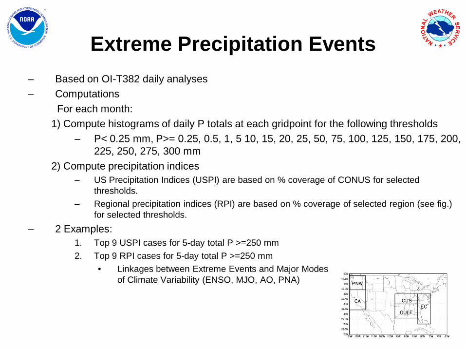
Extreme Precipitation Events– Based on OI-T382 daily analyses– Computations

For each month:1) Compute histograms of daily P totals at each gridpoint for the following thresholds

– P< 0.25 mm, P>= 0.25, 0.5, 1, 5 10, 15, 20, 25, 50, 75, 100, 125, 150, 175, 200, 225, 250, 275, 300 mm

2) Compute precipitation indices– US Precipitation Indices (USPI) are based on % coverage of CONUS for selected

thresholds.– Regional precipitation indices (RPI) are based on % coverage of selected region (see fig.)

for selected thresholds.– 2 Examples:

1. Top 9 USPI cases for 5-day total P >=250 mm 2. Top 9 RPI cases for 5-day total P >=250 mm

• Linkages between Extreme Events and Major Modes of Climate Variability (ENSO, MJO, AO, PNA)

33

Extreme Precipitation Events(Top 9 USPI cases for 5-day total P >=250 mm)

15-19 Feb 1986; USPI = 87

29 Sep-3 Oct 1986; USPI=85

4-8 Nov 2006; USPI = 71

1

2

3

7-11 Jan 1995; USPI = 62

4

29 Dec 96 -2 Jan 97; USPI=61

5

6

27 Jun -1 Jul 1989 USPI = 52

T.S. Allison; During ENSO neutral

6-10 June 2001; USPI = 51

7

Also T.S. Allison;During ENSO neutral

5-9 Feb 1996; USPI = 49

11-15 Sep 1998 ; USPI = 48

T.S. Frances;During La Niña

8

9

During ENSO neutral

During El Niño

During El Niño

During El Niño

During ENSO neutral During La Niña

34

Regional Precipitation Index: Extreme Cases

August 2009

35

Extreme Precipitation Events

36

Pacific Northwest

• Top 8 cases – based on percent coverage of 5-day totals equal to or exceeding 125 mm.– 25 November 1998 (30.8%)– 2 January 1997 (30.6%)– 8 November 2006 (30.2%)– 9 February 1996 (29.8%)– 10 January 1990 (28.4%)– 17 February 1982 (24.4%)– 29 December 1998 (24.0%)– 10 December 1987 (23.4%)

37

RPI125=30.8 RPI125=30.6 RPI125=30.2 RPI125=29.8

RPI125=28.4 RPI125=24.4 RPI125=24.0 RPI125=23.4

38

21-25 Nov98 29 Dec96-2 Jan97 4-8 Nov06 5-9 Feb96

6-10 Jan90 13-17 Feb82 25-29 Dec98 6-10 Dec87

All extreme event cases for the Pacific Northwest feature strong southwest 500-hPa flow into the region. In most cases this flow regime is accompanied by below-average 500-hPa heights over the Gulf of Alaska and western Canada and above-average heights from the Southwest U.S. northeastward into the central U.S.

39

Pacific Northwest

• Top 8 cases – based on percent coverage of 5-day totals equal to or exceeding 250 mm.– 8 November 206 (13.5%)– 9 February 1996 (9.9%)– 18 December 1979 (5.2%)– 17 February 1982 (3.6%)– 25 November 1990 (3.4%)– 8 January 1983 (3.2%)– 1 December 1995 (3.0%)– 31 January 1992 (2.6%)

40

RPI250=13.5 RPI250=9.9 RPI250=5.2 RPI250=3.6

RPI250=3.4 RPI250=3.2 RPI250=3.0 RPI250=2.6

41

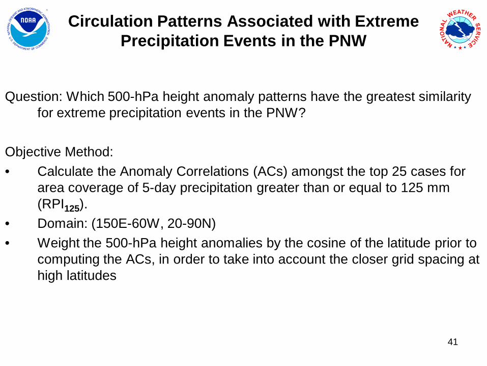
Circulation Patterns Associated with Extreme Precipitation Events in the PNW

Question: Which 500-hPa height anomaly patterns have the greatest similarity for extreme precipitation events in the PNW?

Objective Method:• Calculate the Anomaly Correlations (ACs) amongst the top 25 cases for

area coverage of 5-day precipitation greater than or equal to 125 mm (RPI125).

• Domain: (150E-60W, 20-90N)• Weight the 500-hPa height anomalies by the cosine of the latitude prior to

computing the ACs, in order to take into account the closer grid spacing at high latitudes

42

500-hPa Anomaly Pattern Correlations (x100) for top 25 cases (RPI125).

100. 33. 3. 40. 68. 32. 11. 67. -9. 25. 26. 21. 29. 57. 34. -14. 59. 61. 1. 78. 63. 32. 20. -13. -8.33. 100. 59. 24. 22. 65. 26. 24. 30. 25. 48. 19. 5. 11. -15. 61. 4. 6. 59. 34. 29. 24. 20. 1. 7.3. 59. 100. 36. 9. 75. 46. -9. 64. 20. 37. 58. 26. 8. -19. 76. -15. -2. 65. 3. 10. 34. 20. 29. -31.

40. 24. 36. 100. 55. 62. -3. 47. -6. 55. 37. 54. 55. 29. 4. 23. 39. 48. 56. 32. 46. 73. -8. -19. -33.68. 22. 9. 55. 100. 41. 12. 52. -11. 24. 8. 52. 41. 64. 25. -12. 33. 45. 11. 54. 63. 55. 11. -21. -33.32. 65. 75. 62. 41. 100. 36. 17. 51. 20. 27. 66. 33. 24. -15. 53. -2. 17. 67. 21. 38. 53. 31. 9. -45.11. 26. 46. -3. 12. 36. 100. -42. 66. -21. 10. 39. 29. 5. 27. 46. -33. -13. 30. -3. 2. -7. 22. 76. -28.67. 24. -9. 47. 52. 17. -42. 100. -48. 56. 25. 0. 9. 41. 17. -24. 80. 68. 4. 78. 66. 39. 0. -48. 27.-9. 30. 64. -6. -11. 51. 66. -48. 100. -16. 10. 44. 5. -6. -4. 63. -32. -9. 32. -31. -26. -14. 39. 58. -33.25. 25. 20. 55. 24. 20. -21. 56. -16. 100. 69. 16. 40. 24. 17. 23. 52. 40. 25. 33. 12. 42. -42. -21. 28.26. 48. 37. 37. 8. 27. 10. 25. 10. 69. 100. 12. 43. -2. 27. 50. 30. 6. 30. 13. -9. 18. -44. 7. 12.21. 19. 58. 54. 52. 66. 39. 0. 44. 16. 12. 100. 64. 52. 2. 21. -13. 15. 39. -1. 22. 65. 16. 17. -55.29. 5. 26. 55. 41. 33. 29. 9. 5. 40. 43. 64. 100. 31. 33. 11. 10. 12. 33. 7. 17. 60. -37. 16. -33.57. 11. 8. 29. 64. 24. 5. 41. -6. 24. -2. 52. 31. 100. 1. -28. 17. 33. -12. 48. 47. 59. 12. -28. -17.34. -15. -19. 4. 25. -15. 27. 17. -4. 17. 27. 2. 33. 1. 100. -19. 29. 25. -4. 7. -1. -6. 6. 41. 23.

-14. 61. 76. 23. -12. 53. 46. -24. 63. 23. 50. 21. 11. -28. -19. 100. -13. -9. 64. -9. -14. 2. -3. 36. -13.59. 4. -15. 39. 33. -2. -33. 80. -32. 52. 30. -13. 10. 17. 29. -13. 100. 80. -2. 63. 44. 7. -7. -26. 23.61. 6. -2. 48. 45. 17. -13. 68. -9. 40. 6. 15. 12. 33. 25. -9. 80. 100. 19. 60. 57. 24. 28. -12. 11.1. 59. 65. 56. 11. 67. 30. 4. 32. 25. 30. 39. 33. -12. -4. 64. -2. 19. 100. 6. 26. 48. 16. 25. -15.

78. 34. 3. 32. 54. 21. -3. 78. -31. 33. 13. -1. 7. 48. 7. -9. 63. 60. 6. 100. 75. 31. 9. -25. 11.63. 29. 10. 46. 63. 38. 2. 66. -26. 12. -9. 22. 17. 47. -1. -14. 44. 57. 26. 75. 100. 49. 23. -24. -12.32. 24. 34. 73. 55. 53. -7. 39. -14. 42. 18. 65. 60. 59. -6. 2. 7. 24. 48. 31. 49. 100. -6. -30. -28.20. 20. 20. -8. 11. 31. 22. 0. 39. -42. -44. 16. -37. 12. 6. -3. -7. 28. 16. 9. 23. -6. 100. 18. -5.

-13. 1. 29. -19. -21. 9. 76. -48. 58. -21. 7. 17. 16. -28. 41. 36. -26. -12. 25. -25. -24. -30. 18. 100. 1.-8. 7. -31. -33. -33. -45. -28. 27. -33. 28. 12. -55. -33. -17. 23. -13. 23. 11. -15. 11. -12. -28. -5. 1. 100.

• Patterns 5 and 6 have the largest number of other patterns with AC >=+0.5 (8 in each case, with 3 cases common to both groups).

• Together these two patterns have AC >=+0.5 with 15 (60%) of the patterns.What do these patterns look like?

43

5-9 February 1996

R=0.62

15-19 February 1981

R=0.53

4-8 January 1983

R=0.66

Pattern 6 “Blocking”

13-17 February 1982

29 Dec96-2 Jan97

R=0.65

4-8 November 2006

R=0.75

21-25 February 1986

R=0.67

22-26 December 1980

R=0.53

27 Nov-1 Dec 1995

R=0.51Block over AK/GOA with deep trough and southwesterly flow into west coast

44

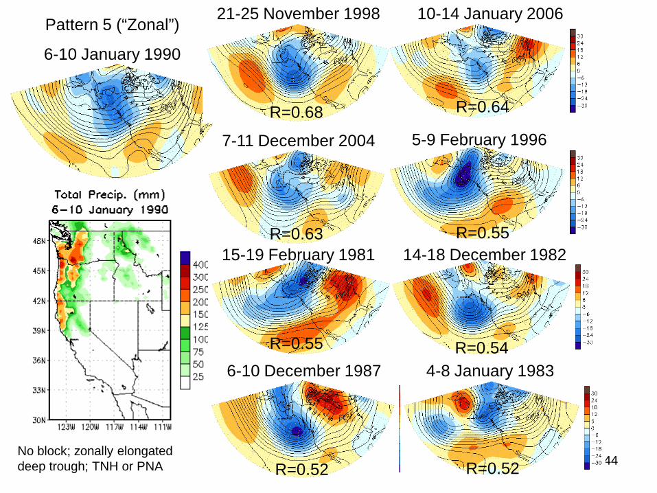
Pattern 5 (“Zonal”)

6-10 January 1990

21-25 November 1998

R=0.68

10-14 January 2006

R=0.64

7-11 December 2004

R=0.63

5-9 February 1996

R=0.5515-19 February 1981

R=0.55

14-18 December 1982

R=0.546-10 December 1987

R=0.52

4-8 January 1983

R=0.52No block; zonally elongated deep trough; TNH or PNA

45


Questions: How often do patterns 5 or 6 occur without 5-day precipitation greater than 125 mm in the PNW?

Objective Method:• Compute the ACs between the reference patterns (5 & 6) and all 5-d ave

height anomaly patterns in the historical record 1979-2006. • Determine:

a. Total number of cases with AC>=0.50b. Total number of cases with AC>=0.50 and RPI125>0 (i.e. 5 day rainfall

amounts greater than or equal to 125 mm somewhere in the region) c. Ratio (b/a) gives hit rate d. Show results by month

46


Pattern 5 (“Zonal”)

6-10 January 1990

Pattern 6 “Blocking”

13-17 February 1982

47

Summary:• When the observed 5-d 500 height anomaly patterns have an AC>=0.50 with either

patterns 5 or 6, there is a 70-98% chance that the PNW will experience 5-d rainfall amounts greater than or equal to 125 mm somewhere in the region.

• The results are remarkably better for the blocking pattern (pattern 6), presumably due to the tendency for blocks to produce more persistent flow over a period of several days.

• There are many extreme rainfall event days that are not captured by patterns 5 & 6 at the AC threshold of 0.50. However, these patterns individually are related to less than 20% (approx 65 out of 350) of the total number of extreme event days during the cool season.

Conclusion:• When either of these two patterns exist during Nov-Feb (Mar) the odds of having an

extreme event are very high. Next step:• Examine the composite evolution of the circulation and patterns of tropical

convection keyed to patterns 5 and 6. Look for connections to MJO, ENSO. • Examine to what extent we can forecast patterns 5 or 6 during Nov- Feb (Mar). Plan to

use CFS V2 reforecast datasets and validation / verification of operational CFS V2 forecasts to look at this question.


intercomparison of daily precipitation statistics over the us...

Documents