Banafsheh Barabadi

Yogendra K. Joshi1

Satish Kumar

G.W. Woodruff School of

Mechanical Engineering,

Georgia Institute of Technology,

Atlanta, GA, 30332

Gamal Refai-AhmedAdvanced Micro Devices, Inc.,

Markham, ON, Canada, L3T-7X6

Interconnect Joule Heatingunder Transient Currentsusing the Transmission LineMatrix MethodThe quality and reliability of interconnects in microelectronics is a major challenge con-sidering the increasing level of integration and high current densities. This work studiedthe problem of transient Joule heating in interconnects in a two-dimensional (2D) inho-mogeneous domain using the transmission line matrix (TLM) method. Computational effi-ciency of the TLM method and its ability to accept non-uniform 2D and 3D mesh andvariable time step makes it a good candidate for multi-scale analysis of Joule heating inon-chip interconnects. The TLM method was implemented with link-resistor (LR) andlink-line (LL) formulations, and the results were compared with a finite element (FE)model. The overall behavior of the TLM models were in good agreement with the FEmodel while, near the heat source, the transient TLM solutions developed slower than theFE solution. The steady-state results of the TLM and FE models were identical. The twoTLM formulations yielded slightly different transient results, with the LL result growingslower, particularly at the source boundary and becoming unstable at short time-steps. Itwas concluded that the LR formulation is more accurate for transient thermal analysis.[DOI: 10.1115/1.4006137]

Keywords: Joule heating, transient, thermal modeling

Introduction

A major concern in the design of microprocessors is the qualityand reliability of on-chip interconnects [1]. These interconnectsare usually Al-Cu- or Cu-based submicron lines deposited on aninsulation layer. Because of the increasing level of integration inmicroprocessors, interconnects are subjected to high current den-sity and; hence, to high temperature increase under operating con-ditions. Moreover, because of the large thermal expansionmismatch between the metallic line and the underlying dielectriclayer, high thermomechanical stresses develop. Several experi-mental and computational studies suggest that these factors areprimarily responsible for morphological changes in the lines thatresult in open-circuit and short-circuit failures in interconnectsand as a consequence, limiting the quality and reliability of theentire circuit. As an example, the basic elements of thermome-chanical fatigue behavior of microelectronic interconnect struc-tures, such as lines and vias, based on accelerated test results havebeen studied and FE analysis has been developed [2].

Interconnect lines always contain a variety of pre-existingdefects such as voids and cracks [3]. Local hot spots, which origi-nate from these defects, often have a major role in controlling themicro-mechanisms of interconnect line failures. Such failure proc-esses are governed by the kinetics of inhomogeneous diffusionsand/or reactions. For example, the effect of electromigration, aswell as the variation of diffusion rates, will accelerate void growthand translation, and their accompanied stress buildups, leading toa final failure of the interconnect line. The transient heat transferin the system greatly influences the morphology of failure and thepattern of damage evolution, which depend strongly on the elec-tric current loading rate.

The problem of steady state Joule heating in interconnects hasbeen studied using 2D analytical, finite difference (FD), and finiteelement (FE) 2D and 3D models [4–6]. Multi-stack interconnectarchitecture is characterized by wide range of length scales(from 10�9 m to 10�2 m) and significant material inhomogeneity(thermal conductivity variation from 0.1 W/mK to 400 W/mK).Different metal levels are connected through vias that provideelectrical connections. To reduce the total simulation time, it isoften desirable to use an inhomogeneous mesh that is more refinedin the areas if there is large temperature gradient. In existing FDand FE models, computational times are long even for a unit cell(micro-models). Some authors have proposed compact FE modelsto reduce the computational time, with the trade-off being reducedresolution and accuracy especially at the interface between themetal and dielectric [7,8]. It has been shown that using the methodof quad-tree mesh with the TLM method as well as algorithms foroptimizing the time stepping can reduces the execution time by100 times [9].

Recent multicore chip architectures which incorporate dynamicmigration of computing loads point to the importance of Jouleheating under transient conditions. In the present study, we inves-tigate transient heating effects using the Transmission Line Matrix(TLM) Method [10,11]. The TLM formulation is based on a re-sistance and capacitance network and allows for temperature-dependent and inhomogeneous material parameters, non-uniformmesh, and variable time-stepping. The conventional link-line (LL)TLM network used for 1D diffusion problems often results in nu-merical oscillations [12]. The link resistor (LR) method, with ca-pacitance centered on the nodes, with resistors placed mid-waybetween nodes, contrasts with the LL method, in which resistorsare placed at the nodes, with transmission lines linking adjacentnodes, yielding reduced oscillations. Comparisons between vari-ous LL and LR models indicate that, in general, 2D LR TLMmodels consistently produce more accurate results [12]. It shouldbe noted that, once the domain is approximated by a TLM model,the TLM solution is exact. The approximation of a TLM model isin the analogy of the physical system (in this case, heat diffusion)with an electrical circuit. In contrast, two approximations exist in

1Corresponding author. Yogendra K. Joshi, Ph.D., G.W. Woodruff School ofMechanical Engineering, Georgia Institute of Technology, 801 Ferst Dr, Atlanta,GA, 30332.

Contributed by the Electronic and Photonic Packaging Division of ASME forpublication in the JOURNAL OF ELECTRONIC PACKAGING. Manuscript received July 19,2010; final manuscript received December 2, 2011; published online March 21,2012. Assoc. Editor: Koneru Ramakrishna.

Journal of Electronic Packaging MARCH 2012, Vol. 134 / 011009-1Copyright VC 2012 by ASME

Downloaded From: http://electronicpackaging.asmedigitalcollection.asme.org/ on 01/08/2014 Terms of Use: http://asme.org/terms

the FE model: one approximation is in dividing the given geome-try into elements, the other is in approximating the solution in anelement. It is important to note that nonlinear material properties,dependent on time or temperature, can be implemented in theTLM algorithm as described by several authors in the literature(e.g., Refs. [10] and [11]).

Another advantage of the TLM method over FD and FE meth-ods is greater stability. In particular, for transient thermal analysis,this allows the time step to be increased as the simulation pro-gresses towards steady state; hence reducing the computationaltime significantly. Moreover, TLM has the possible use in multi-scale simulations by incorporating rapid local zoom-in approachessuch as the quad-tree mesh [9–11].

TLM Background

The original TLM differential equation is a hyperbolic equa-tion, which indicates that this method can also be used to simulatethe hyperbolic heat equation that is based on the Cattaneo equa-tion. The Cattaneo equation has been proposed as a more generalform of Fourier’s law and many researchers believe that Catta-neo’s equation extends the validation regime of Fourier’s law totime scales shorter than the relaxation time of a material. Catta-neo’s equation leads to a form of heat equation known as thehyperbolic heat equation, which is a damped wave equation thatpredicts heat will propagate in waves with a finite speed. How-ever, because of the lack of convincing experimental evidenceand contradictions with the second law of thermodynamics, justifi-cation for accepting Cattaneo’s equation has been questioned[13]. Several phenomenological theories have been developed todescribe transient heat transfer processes in solids and micro-/nano-structures. Applications of transient and ultra-fast heatinginclude laser processing, nanothermal fabrication, and the mea-surement of thermophysical properties. In the literature, thereappears to be controversial experimental evidence on the exis-tence of certain phenomena predicted by the hyperbolic heat con-duction. Furthermore, there exists a large division regarding theformulation and the interpretation of the theories of non-Fourierconduction. Consequently, to avoid the issues associated withhyperbolic heat conduction equation, the propagation term in Eq.(1) is kept small and negligible (see below), such that the analo-gous heat equation (Eq. (5)) can be approximated. As described inthe following section, this is verified with keeping the parameterm much smaller than unity.

Formulation

An electrical impulse in a transmission line matrix can be for-mulated using the Maxwell’s curl equation for propagation in alossy medium, also known as the Telegrapher’s Equation [14]:

r2V ¼ LdCd@2V

@t2þ RdCd

@V

@t� Rd

DxI (1)

where, Ld, Cd, and Rd are the distributed electrical inductance, ca-pacitance, and resistance per unit length in the transmission line,respectively. V and I are the nodal voltage and current in the elec-trical circuit.

Eq. (1) and transient heat conduction equation (Eq. (5)) have asimilar structure. In Eq. (1), voltage can be treated as temperature(V : T) and a network of electrical circuit elements can simulatethe medium, which means that temperature propagates in the formof a damped wave. This is only valid on the grounds that the spaceand time discretizations are properly chosen (explained in thissection). Using this approach, the transient heat conduction equa-tion can be solved explicitly. Some advantages of this method canbe found in Refs. [10,11]. Analytical solution of the transient heatconduction equation for interconnects is complicated due to: (a)non-continuum transport effects at sub 40 nm for copper, (b) tran-sient heat transfer at short-time scales associated with device

operational frequencies, (c) the large variation in thermal proper-ties of the material from metals to dielectrics, and (d) the non-uniformity of heat generation at the base of devices [13]. TLMbased formulation is of great value in simulations involvingmicro/nano-length and -time scales, variation in thermal proper-ties and non-uniform power generation. The physical interpreta-tion of the coefficients of Eq. (1) is related to the thermalparameters as described in the following analogies:

RdCd �1

a¼ qCP

j(2)

where a is the diffusion coefficient, and

LdCd �1

v2tw

(3)

where vtw is the speed of the temperature wave. By dividing Eq.(3) by Eq. (2), it can be seen that the relaxation time of the tem-perature wave, which is interpreted as the time of the collision ofthe particles [13], can be written as

s � LdCd

RdCd¼ Ld

Rd(4)

By substituting the thermal equivalence of the parameters backinto the Eq. (1), the Telegrapher’s Equation can be reduced to thetransient heat conduction equation:

r jðTÞrTð Þ ¼ qCP@T

@t� gðx; y; z; tÞ (5)

where j(T) is the thermal conductivity as a function of tempera-ture, Cp is the specific heat of the material, q is the material den-sity, and g(x,y,z,t) represents the local instantaneous volumetricheat generation.

Notably, the first term on the right-hand side of Eq. (1), thepropagation term, has no equivalent in the classical heat diffusionequation (Eq. (5)), and is therefore an error term in transmissionline modeling of diffusion problems. The error term is negligiblewhen [15]

RdCd@V

@t>> LdCd

@2V

@t2(6)

By defining the parameter m as

m ¼ LdCd@2V

@t2

�RdCd

@V

@t(7)

The restriction in Eq. (6) can be restated as m� 1. The errorparameter m, for a 2D heat diffusion problem with diffusion coef-ficient a, can be written as [15]

m ¼ aDt2

Dx2

@2V

@t2

�@V

@t

� �(8)

which shows that m is a function of both time step and spatial re-solution. The parameter m is a measure of how accurately the Tel-egrapher’s equation (Eq. (1)) models the diffusion equation. It isnot a measure of the accuracy of the numerical solution to the par-ticular problem, which ultimately depends on the spatial resolu-tion and time step, Dx and Dt. The parameter m allowsdetermination of an appropriate choice of Dt for the Dx beingemployed.

Once Rd and Cd have been determined by the physical problem,a requirement that the pulses travel from node to node in a time

011009-2 / Vol. 134, MARCH 2012 Transactions of the ASME

Downloaded From: http://electronicpackaging.asmedigitalcollection.asme.org/ on 01/08/2014 Terms of Use: http://asme.org/terms

step Dt results in the complex transmission line impedance Zbeing equal to Dt/(CdDx), where Dx is the local distance betweennodes. The requirement that the second term in Eq. (1) be negligi-ble then becomes a condition that Dt must be sufficiently small[9].

Methodology

The TLM approach is described here primarily following[10,11]. The TLM method is built on the rules governing thetravel of potential pulses. In a 1D horizontal model (Fig. 1), theincident pulse at an arbitrary node (x) travels along the transmis-sion lines approaching the node from either left or right. Thispulse will then be scattered passing the node. It either getsreflected back in the same line with the reflection coefficient q, orgets transmitted with the transmission coefficient s. These coeffi-cients are calculated based on the encountered resistance and im-pedance on the transmission line. A voltage impulse entering a LLnode will travel along a transmission line during a time Dt/2. Atthis point, it encounters a discontinuity, ZT¼ (RþRþZ). Thereflection coefficient q¼ (ZT – Z)/(ZTþZ) is then

q ¼ R

Rþ Z(9)

Based on the fact that qþ s¼ 1, the transmission coefficient willbe

s ¼ Z

Rþ Z(10)

The equivalent discretizations of the medium are analogous elec-trical network methods shown in Figs. 1(a) and 1(c). If the impe-dances are located at the interface between the nodes, it is called aLink-line (LL) representation (Fig. 1(b)). On the other hand, if theresistors are placed at the interface, it is called a Link-Resistor (LR)representation, which is implemented in the present work andshown in Fig. 1(d). To write the equation of transmission line based

on the electrical equivalent circuit, we focus on the three adjacentnodes in the line (x), (xþ 1), and (x� 1) demonstrated in Fig. 2. Atthe start of an iteration, six pulses share these three positions, whichare situated at the center of transmission lines. The interaction ofthese waves is described below and in Fig. 2.

The incident pulses from left and right for node (x) at any timestep are a combination of the pulses that have been scattered atthe previous time step from the adjacent nodes and node (x) itself.In other words, the pulse that is at (x� 1) traveling to the left is nolonger relevant to node (x) and is ignored. The same applies to theone that is traveling to the right from (xþ 1). These two pulses areshown with dotted line arrows. The other four pulses travel fortime Dt/2 before they are scattered at the resistors. They areshown as dashed line arrows. They then become incident on (x)from left and right, shown with solid line arrows. The formulationwill then be in the forms of:

(a) Incident pulse for node (x) at time step kþ 1:

kþ1iVLðxÞ ¼ qs

kVLðxÞ þ sskVRðx� 1Þ

kþ1iVRðxÞ ¼ qs

kVRðxÞ þ sskVLðxþ 1Þ

(11)

(b) Scattered pulse for node (x) at time step kþ 1. When anincident pulse passes a node from one side to another, itswitches from incident to scattered:

skþ1VLðxÞ ¼i

kþ1VRðxÞskþ1VRðxÞ ¼i

kþ1VLðxÞ(12)

(c) Instantaneous potential at node (x) at time step kþ 1 iswritten as the summation of simultaneously arrivingpulses at the node:

kþ1V ¼ikþ1VLðxÞ þi

kþ1VRðxÞ (13)

To complete the algorithm, Eqs. (11) – (13) are repeated for kiterations, where kDt is the total time of simulation.

Two types of boundary conditions (BCs) were considered in thiswork. As a heat pulse reaches an insulating boundary, it gets reflectedback into the physical domain. This is equivalent to an open-circuit(q¼ 1) condition. This condition should be applied at the interfacebetween nodes. Hence, a pulse traveling from a node during time Dt/2 faces the boundary and arrives back at the node at the end of thetime step. Assuming there is an insulating boundary on the right-handside of the 1D model, using Eq. (11), this BC can be formulated as:

ikþ1VLðxÞ ¼ qs

kVLðxÞ þ sskVRðx� 1Þ (14)

ikþ1VRðxÞ ¼ 1s

kVRðxÞ þ 0skVLðxþ 1Þ (15)

Eq. (15) can be simplified:

kþ1iVRðxÞ ¼s

k VRðxÞ (16)

For a constant temperature boundary, it is the resistor – not thetransmission line – that touches the boundary. There are two

Fig. 1 Analogous electrical circuit for (a) link-line TLM (LL TLM)method and (c) link-resistor TLM (LR TLM) method. Electrical cir-cuit representation of a single node of resistance-impedancenetwork by (b) LL TLM and (d) LR TLM methods [11].

Fig. 2 Three adjacent nodes located at the center of transmission line and theirpulses. Solid line arrows 5 incident pulse. Dashed and dotted line arrows 5 scatteredpulse. Pulse notation for left superscript: s 5 scattered and i 5 incident. Pulse nota-tion for left subscript: k 5 time step. Pulse notation for right subscript: pulseapproaching the node from left (L) and from right (R).

Journal of Electronic Packaging MARCH 2012, Vol. 134 / 011009-3

Downloaded From: http://electronicpackaging.asmedigitalcollection.asme.org/ on 01/08/2014 Terms of Use: http://asme.org/terms

separate considerations in this BC: (a) the input from the sourcecan now be placed at the boundary, and (b) the history of the pulsethat is scattered from node 1 subsequently approaches the bound-ary. The source (VC) on the boundary sees a series connection ofresistor and impedance, so the standard potential divider formulagives the signal injected into the line. The pulse scattered towardthe boundary sees a short circuit, so the total, which is incidentfrom the left at a new time step, is the sum of these contributions.This can be formulated as

kþ1iVLð1Þ ¼ VC

Z

Rþ Z

� �þs

k VLð1ÞR� Z

Rþ Z

� �(17)

In the LL method, Eqs. (11), (12), and (13) are replaced by the fol-lowing equations:

(a) At time k, two incident pulses travel along the transmis-sion line and approach the center of the node (x) fromleft and right. We can write Eq. (13) for time k:

kV ¼ik VLðxÞ þi

k VRðxÞ (18)

(b) Scattered pulse (reflection and transmission) for node (x)at time step k:

skVLðxÞ ¼ qi

kVLðxÞ þ sikVRðxÞ

skVRðxÞ ¼ si

kVLðxÞ þ qikVRðxÞ

(19)

(c) Incident pulse for node (x) at time step kþ 1. Each scat-tered pulse travels to the boundaries and becomes anincident pulse at the adjacent nodes:

kþ1iVLðxÞ ¼s

k VRðx� 1Þkþ!

iVRðxÞ ¼sk VLðxþ 1Þ

(20)

The iterative implementation of Eqs. (18) - (20) forms the LLalgorithm. It is clear that the main difference between the LR andLL methods is in the calculation of incident and scattered pulses(i.e., Eqs. (11) and (19)). An insulating BC at the right end will bethe same as described in Eq. (16). The formulation of theconstant-temperature boundary, however, is different for LL andLR models. In an LL model, the transmission line touches theboundary. To keep a constant temperature VC at the left boundary,a “fictitious” node outside the boundary is assumed together withits corresponding source and transmission line. The temperature atthe surface is calculated from the summation of the pulse incidenton node 1 at each new time step, and the pulse scattered fromnode 1 at the previous time step, which should stay constant:

kþ1iVLð1Þ ¼ �1s

kVLð1Þ þ VC (21)

Since the right-hand side of Eq. (21) is known at the presenttime step, the incident pulse approaching node (x) from the leftcan be calculated.

2D TLM algorithms follow the general principles discussed inEqs. (11) to (21) for two perpendicular transmission lines. Follow-ing Ref. [12], two TLM codes were developed for LR and LL for-mulations and implemented in MATLAB for the following casestudy. A finite difference expression was used in the derivation ofm for each node (n) at each time step (k). Following Ref. [15], themean values of the backward difference forms of the time deriva-tives were employed to reduce numerical oscillations:

kmðnÞ ¼ a2

Dt2

Dx2

½kVðnÞ þk�1 VðnÞ� � 2½k�2VðnÞ þk�3 VðnÞ� þ ½k�4VðnÞ þk�5 VðnÞ�½kVðnÞ þk�1 VðnÞ� � ½k�2VðnÞ þk�3 VðnÞ�

(22)

To avoid storing several generations of nodal temperatures at allthe nodes, the values of m were calculated at two representativenodes with higher temperatures, one in the interconnect and onein the dielectric.

2D Case Study

A simple case study of interconnect temperature increase forthe structure seen in Fig. 3 was performed to evaluate the TLMmodeling approach. Simulations of this configuration using FEwere used as a basis for the evaluation of the TLM results. Thisstructure closely approximates long, uniformly spaced intercon-nects [8]. The interconnect aspect ratio is close to 2 for structuresfound in microprocessors (Hint¼ 2W) and the dielectric thicknessis approximately equal to the interconnect height (Hd¼ 2W).Interconnect pitch P is variable; we took P¼ 4W in this study.The bottom surface is fixed at a constant temperature (T¼ 0) andall other surfaces are assumed to be adiabatic. The continuumassumption of our modeling approach was verified by calculatingthe Knudsen number:

Kn ¼ kL

(23)

where k is the molecular mean free path and L the smallest lengthscale in the problem [13]. The continuum approach is valid aslong as Kn� 1.0. We calculate Kn¼ 0.22 based on the mean freepath of copper molecules at 20 �C (k¼ 39 nm) and the width ofinterconnects (L¼ 180 nm); this justifies that the continuumapproach is valid.

The FE model consists of 561 nodes (17� 33) and 512 ele-ments. The TLM nodes were selected at the center of FE elements(512 nodes). The interconnect width chosen was W¼ 180 nm,similar to the interconnect width in Ref. [8]. The material proper-ties for the metal and dielectric were specific heat capacityCh¼ 380 and 1000 J/kgK, density q¼ 8933 and 2200 kg/m3, andthermal conductivity j¼ 400 and 0.17 W/mK, respectively. Thecomparisons made in this study are for a case when the left-mostinterconnect is carrying a current density of 10 MA/cm2 and thevolumetric heat generation is 2.2� 1014 W/m3 which is calculatedusing a resistivity of 2.2 lX-cm.

The FE solver LSDyna (LSTC, Livermore, Calif., USA) fornonlinear multi-physics problems is used, with a variable timestep Crank-Nicholson scheme. The FE solver was validated in a

Fig. 3 Schematic of the model consisting of a set of W 5 180nm wide interconnects that are evenly spaced and embedded inthe dielectric. The mesh used in the FEA technique is shown. Inthis study: Hint 5 Hd 5 2W and P 5 4W.

011009-4 / Vol. 134, MARCH 2012 Transactions of the ASME

Downloaded From: http://electronicpackaging.asmedigitalcollection.asme.org/ on 01/08/2014 Terms of Use: http://asme.org/terms

homogenous 2D problem for which an analytical solution existed[9]. The time step for FE simulations was 1.72 ns.

At each TLM node, considering the inhomogeneity of themodel, the resistance and capacitance were defined as [12]

Rðx; yÞ ¼ 0:5dx

Ajðx; yÞ (24)

Cðx; yÞ ¼ Adxqðx; yÞChðx; yÞ (25)

where dx is the length and A is the cross-sectional area of eachelement, with the thickness equal to 1 lm. The impedance at eachnode was, therefore,

Zðx; yÞ ¼ dt

0:5Cðx; yÞ (26)

The thermal time constant RC of the dielectric material was 25 ns.The TLM time step was chosen smaller than the minimum ther-mal time constant, i.e., dt¼ 10, 1.0, and 0.1 ns. For comparison,the TLM and FE results were stored at every 1 ls.

The source term in the TLM model was

Vexðx; yÞ ¼1

4AdxIðx; yÞZðx; yÞ (27)

for the LR model and

Vexðx; yÞ ¼1

4AdxIðx; yÞ Zðx; yÞ þ Rðx; yÞ½ � (28)

for the LL model. In Eqs. (27) and (28), I(x, y) is the volumetric heatsource. Vex was added to the nodal temperatures at each iteration.

Results and Comparison

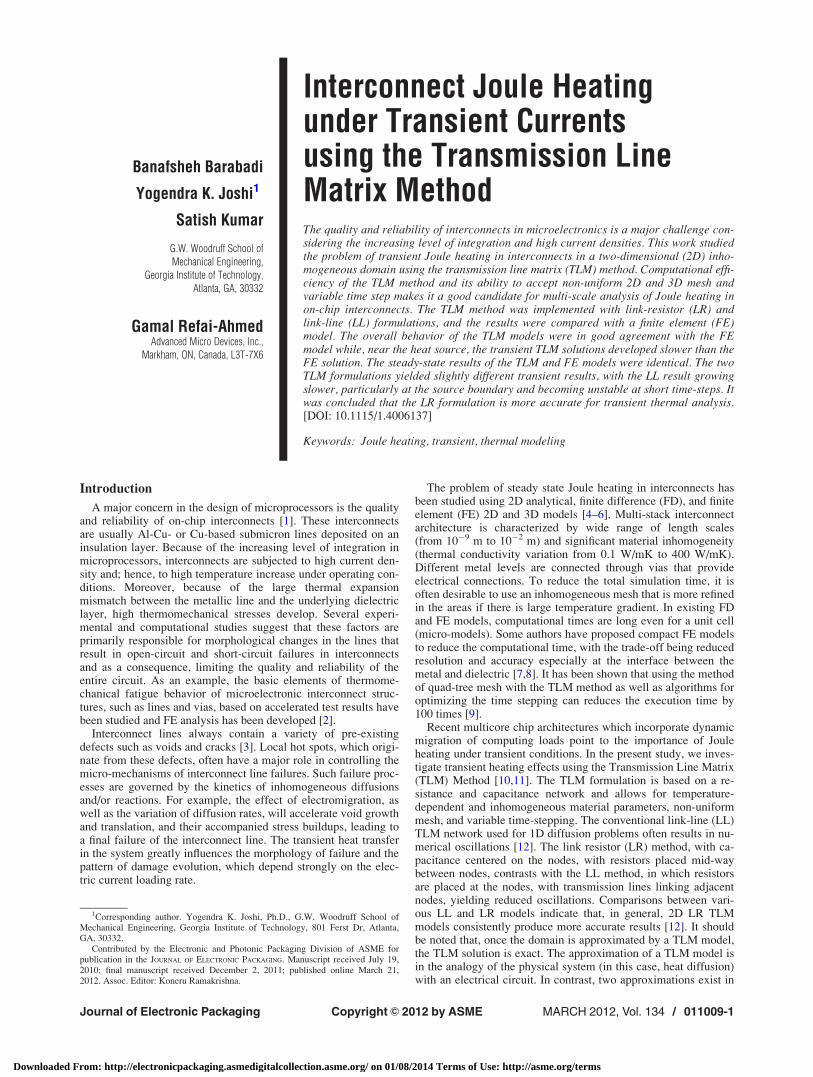
Figures 4(a) and 4(b) show the results for the spatial variationof temperature at 14 ls from FE and LR TLM respectively.As expected, heat propagates through the structure from left toright and top to bottom due to the heat source at the left-most

interconnect. The temperature within an interconnect stays almostconstant due to its relatively high conductivity. Due to theadiabatic boundary conditions, the temperature contours are per-pendicular to the top and left edges.

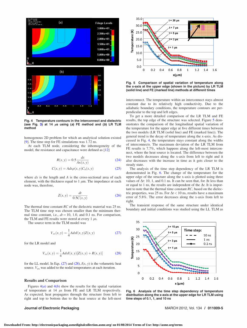
To get a more detailed comparison of the LR TLM and FEresults, the top edge of the structure was selected. Figure 5 dem-onstrates the comparison of the longitudinal spatial variation ofthe temperature for the upper edge at five different times betweenthe two models (LR TLM (solid line) and FE (marked line)). Thegeneral trend is the decay of temperature along the x-axis. As dis-cussed in Fig. 4, the temperature stays constant along the widthsof interconnects. The maximum deviation of the LR TLM fromFE results is 7.7%, which happens along the left-most intercon-nect, where the heat source is located. The difference between thetwo models decreases along the x-axis from left to right and italso decreases with the increase in time as it gets closer to thesteady state.

The analysis of the time step dependency of the LR TLM isdemonstrated in Fig. 6. The change of the temperature for theupper edge of the structure along the x-axis is plotted using threevalues of Dt: 10, 1, and 0.1 ns. It can be seen that, for Dt less thanor equal to 1 ns, the results are independent of the Dt. It is impor-tant to note that the thermal time constant RC, based on the dielec-tric properties, was 25 ns. For Dt< 10 ns, results have a maximumerror of 5.8%. The error decreases along the x-axis from left toright.

The transient response of the same structure under identicalboundary and initial conditions was studied using the LL TLM as

Fig. 4 Temperature contours in the interconnect and dielectric(see Fig. 3) at 14 ls using (a) FE method and (b) LR TLMmethod

Fig. 5 Comparison of spatial variation of temperature alongthe x-axis at the upper edge (shown in the picture) by LR TLM(solid line) and FE (marked line) methods at different times

Fig. 6 Analysis of the time step dependency of temperaturedistribution along the x-axis at the upper edge for LR TLM usingtime steps of 0.1, 1, and 10 ns

Journal of Electronic Packaging MARCH 2012, Vol. 134 / 011009-5

Downloaded From: http://electronicpackaging.asmedigitalcollection.asme.org/ on 01/08/2014 Terms of Use: http://asme.org/terms

well. Temperature along the x-axis at the upper edge at three dif-ferent times computed from various methods is shown in Fig. 7. Itcan be inferred from this figure that LL TLM grows slower thanLR TLM. In other words, the transient response of LL TLM lags

FE results more than LR TLM and thus, is less accurate. This hasalso been addressed in Ref. [12]. The difference between the twomodels, however, decreases along the x-axis as distance from theheat source increases. It also decreases with time.

One of the other differences between the LL and LR TLM is intheir dependency on Dt. As discussed earlier for LR TLM, for anyDt smaller than about one tenth of the smallest dielectric RC, themodel is independent of Dt. In this study for time-steps between10 ns and 1.92 ns, results are valid and accurate for both models,with a maximum error of 2.8% at steady state. For instance, thevariation of temperature in x-direction throughout the structurewith time step of 1.95 ns and 1.90 ns are demonstrated in Fig. 8(a)and 8(b), respectively. However, for LL TLM, Dt< 1.92 ns causesthe model to become unstable. As demonstrated in Fig. 8(b), theinstability grows from the far right corner of the structure (high-lighted in Fig. 8(c)) and arises closer to the steady-state situation.It can be seen that the instability also happens at an earlier time asthe time step decreases. The source term in the TLM modelsappears to be an important factor in the numerical oscillations andinstabilities mentioned above. Applying smoother input functions,increasing the dimensions of the problem, and using the LR versusLL formulations generally reduce such oscillations [11,12].

The value of m is calculated at two points: the upper-left cor-ner (the interconnect region) and at 90 nm to the right of the firstpoint (the dielectric region). The values of m, root mean square(RMS) over time for dt¼ 1 ns in the LR model, were 0.268 and3.69� 10�5, respectively, which confirmed that the propagationterm in the TLM formulation was negligible. The reason behindchoosing the points mentioned is the high temperatures at theselocations. In implementing the control of Dt using Eq. (22), it isimportant to avoid situations that lead to near-zero values of dV/dt (< 10�8). Therefore, by averaging the values of m withrespect to time, the effect of oscillations was eliminated. TheRMS values of m, for three cases of dt¼ 0.1, 1, and 10 ns aretabulated in Table 1.

The “average computational time” was defined as the ratio ofthe computational time to the simulation time. This ratio was 4.68s/ls for FE simulations. For the LR TLM code it was 1.20 s/ls fordt¼ 10 ns and 11.87 for dt¼ 1 ns. Considering that the TLM codewas running in MATLAB environment, it can be concluded that,with a standalone executable code, the TLM computational timewould decrease.

Discussion and Conclusions

In this study, 2D LR and LL TLM algorithms were imple-mented for transient heat conduction in inhomogeneous arrange-ments of interconnects and dielectrics. A two-dimensional casestudy was presented and the TLM results were compared with thetransient FE results. The overall behavior of the TLM models wassimilar to the FE model while, near the heat source, the transientTLM solutions developed slower than the FE solution. The issueof inaccuracy due to a voltage source being added at the boundaryhas been addressed previously by investigators such as Ref. [12].The steady-state results of the two models were in good agree-ment with a maximum error of 2.8%.

Fig. 7 Comparison of spatial variation of temperature alongthe x-axis at the upper edge by LR TLM (solid line), LL TLM(dashed line), and FE results (marked line) at three differenttimes

Fig. 8 Observation of the time step dependency of the temper-ature in LL TLM method along x-axis throughout the structurewith time steps of (a) Dt 5 1.95 ns and (b) Dt 5 1.9 ns. (c) Sche-matic of structure with highlighted region where the instabilitygrows when time step is less than 1.92 ns.

Table 1 The RMS values of m calculated at two points: theupper-left corner (the interconnect region) and at 90 nm to theright of the first point (the dielectric region) for three cases ofdt 5 0.1, 1, and 10 ns

RMS value of “m”

time step (ns)interconnect

with the sourcedielectric adjacent

to the source

10 ns 15.730 0.0061 ns 0.268 3.69� 10�5

0.1 ns 0.0003 1.96� 10�7

011009-6 / Vol. 134, MARCH 2012 Transactions of the ASME

Downloaded From: http://electronicpackaging.asmedigitalcollection.asme.org/ on 01/08/2014 Terms of Use: http://asme.org/terms

Two distinct TLM formulations, LR and LL, were implementedand compared. The two formulations yielded slightly differenttransient results, with the LL result growing slower, particularly atthe source boundary. The LR formulation results were closer tothe FE results. It was shown that the stability of the LL resultsdepends on the time step. Below a maximum time step, the LLresults showed instability that started from the insulating bound-ary. Similar observations have been reported by Refs. [11] and[12], who indicated that the LR formulation is more accurate fortransient thermal analysis.

An important feature to be added to this study is the use of aspecial type of mesh refinement called quad-tree mesh. Quad-treemesh has the ability to increase the mesh resolution dramaticallyin a rather short length scale and; therefore, to generate a non-uniform mesh along different directions. Using a quad-tree meshwith TLM method, an inhomogeneous multi-scale structure canbe simulated in a reasonable simulation time by having locallyrefined mesh resolution at points of interests.

In the transient solution of heat diffusion equation, the initialtime step should be smaller than the thermal time constant for thephysics of the problem to be captured accurately. However, for aconstant heat source, as the solution reaches the steady state, therate of change of temperature as a function of time decreases. Animportant feature of the TLM model is the ability to accept a vari-able time step. Therefore, by using an adjustable time step duringthe TLM simulation, the computational time can be dramaticallydecreased [9].

Acknowledgment

The funding for this study was provided by SemiconductorResearch Corporation (SRC) under task 1883.001.

References[1] Phan, T., Dilhaire, S., Quintard, V., Lewis, D., and Claeys, W., 1997,

“Thermomechanical Study of AlCu Based Interconnect Under Pulsed Thermo-electric Excitation,” J. Appl. Phys., 81, pp. 1157–1157.

[2] Evans, J. W., Evans, J. Y., Lall, P.,and Cornford, S. L., 1998,“Thermomechanical Failures in Microelectronic Interconnects,” Microelectron.Reliab., 38, pp. 523–529.

[3] Bastawros, A. F., and Kim, K. S., 1998, “Experimental Study on Electric-Current Induced Damage Evolution at the Crack Tip in Thin Film Conductors,”Trans. ASME J. Electron. Packag., 120, pp. 354–359.

[4] Bilotti, A. A., 1974, “Static Temperature Distribution in IC Chips with Isother-mal Heat Sources,” IEEE Trans. Electron Devices, ED-21, pp. 217–226.

[5] Teng, C. C., Cheng, Y.-K., Rosenbaum, E., and Kang, S.-M., 2002, “iTEM: ATemperature-Dependent Electromigration Reliability Diagnosis Tool,” IEEETrans. Comput.-Aided Des., 16, pp. 882–893.

[6] Chen, D. Li, E., Rosenbaum, E., and Kang, S.-M., 2002, “Interconnect ThermalModeling for Accurate Simulation of Circuit Timing and Reliability,” IEEETrans. Comput.-Aided Des., 19, pp. 197–205.

[7] Stan, M. R., Skadron, K., Barcella, M., Huang, W., Sankaranarayana, K., andVelusamy, S., 2003, “HotSpot: A Dynamic Compact Thermal Model at theProcessor-Architecture Level,” Microelectron. J., 34, pp. 1153–1165.

[8] Gurrum, S. P., Joshi, Y. K., King, W. P., Ramakrishna, K., and Gall, M., 2008,“A Compact Approach to On-Chip Interconnect Heat Conduction Modelingusing the Finite Element Method,” J. Electron. Packag., 130, p. 031001.

[9] Smy, T., Walkey, D., and Dew, S. K., 2001, “Transient 3D Heat Flow Analysisfor Integrated Circuit Devices using the Transmission Line Matrix Method on aQuad Tree Mesh,” Solid-State Electron., 45, pp. 1137–1148.

[10] Christopoulos, C., 1995, The Transmission-Line Modeling Method TLM, IEEEPress, New York.

[11] De Cogan, D., O’Connor, W. J., and Pulko, S., 2006, Transmission Line Matrixin Computational Mechanics, CRC, Boca Raton, FL.

[12] Ait-sadi, R., and Naylor, P., 1993, “An Investigation of the Different TLM Con-figurations used in the Modelling of Diffusion Problems,” Int. J. Numer.Model., 6, pp. 253–268.

[13] Zhang, Z. M., 2007, Nano/Microscale Heat Transfer, McGraw-Hill Professio-nal, New York.

[14] Johns, P. B., 1977, “A Simple Explicit and Unconditionally Stable NumericalRoutine for the Solution of the Diffusion Equation,” Int. J. Numer. MethodsEng., 11, pp. 1307–1328.

[15] Gui, X., Webb, P. W., and De Cogan, D., 1992, “An Error Parameter in TLMDiffusion Modelling,” Int. J. Numer. Model., 5, pp. 129–137.

Journal of Electronic Packaging MARCH 2012, Vol. 134 / 011009-7

Downloaded From: http://electronicpackaging.asmedigitalcollection.asme.org/ on 01/08/2014 Terms of Use: http://asme.org/terms