Munich Personal RePEc Archive

International tourism receipts and

economic growth in Kenya 1980 -2013

Akama, Erick

University of Nairobi

12 November 2016

Online at https://mpra.ub.uni-muenchen.de/78110/

MPRA Paper No. 78110, posted 12 Apr 2017 11:51 UTC

INTERNATIONAL TOURISM RECIEPTS AND ECONOMIC GROWTH IN KENYA

1980 -2013

AKAMA ERICK MAIKO

X50/67704/2013

A Research Project Submitted to the School of Economics in Partial Fulfillment of the

Requirement for the Award of Degree of Master of Arts in Economics of the University

of Nairobi.

2016

ii

DECLARATION

I hereby declare that this is my original work and that to the best of my knowledge has never

been presented for the award of any degree in any other university or institution.

CANDIDATE: AKAMA ERICK MAIKO

ADMISION NUMBER: X50/67704/2013

SIGNATURE……………………………………………DATE……………………………

APPROVAL

This MA Research project has been forwarded for examination with my approval as

University Supervisor:

DR. THOMAS ONGORO

SIGNATURE……………………………DATE………………………………………..

iii

DEDICATION

All my dedication goes to my mum (Grace Nyabisi), my wife(Mercy) brothers and sister for

their firm support in encouraging me and constantly reminding me for the value of time for

the duration I was undertaking my studies. Their inspirations and positive advices ensured my

accomplishing of this work. I appreciate them dearly.

iv

ACKNOWLEDGEMENT

It’s my greatest pleasure and humility to thank the following persons for their valuable inputs

in my work. First and foremost, Dr. Thomas Ongoro of UON, thank you very much for your

exemplarily guidance, monitoring and positive critics that led to a standard research paper.

Your value of the duration of a good research paper taught me patience and determination.

Secondly my gratitude goes to the University of Nairobi, School of Economics defense

panelist for their professionalism and convivial support that led to the successful completion

of my research.

My thanks goes also to all my brothers (Evans, Obadiah and Obae), my only sister (Lilian)

and my Mum Grace as well as Dad-David for their moral support and understanding during

this period. They were there for me when I needed them most.

Lastly, I thank in a special way Almighty God for the good health and wisdom during the

duration I was undertaking the research.

Thank you.

v

LIST OF FIGURES

Graph 1: Role of Tourism industry to the global economy in US dollar billions

Graph 2: The share of the Travel and Tourism sector to the world employment in thousands

Graph 3: World GDP growth rate and international receipts growth rate

Graph 4: Kenyan percentage share of GDP by main sector for some selected years

vi

LIST OF TABLES

Table1. Data type, source &Typology of all the variables

Table 2: Descriptive statistics

Table 3: Shapiro-Wilk normality test

Table 4: VIF and Tolerance results

Table 5: ADF test results

Table 6: ADF test results for differenced variables

Table 7: Engle-Granger Test for Cointegration

Table 8: Engle-Granger Test for Cointegration

Table 9: Long run Regression Results in Level

Table 10: Regression Results in First Difference

vii

LIST OF ACRONYMS AND ABBREVIATIONS

UNWTO - United Nations World Tourism Organization

GDP - Gross Domestic Product

ADF - Augmented Dickey-Fuller

KNBS - Kenya National Bureau of Statistics

OLS - Ordinary Least Squares

WTO - World Trade Organization

WTTC - World Travel and Tourism Council

OECD - Organization for economic cooperation and development

VECM - Vector Error Correcting Model

FDI - Foreign Direct Investment

TLGH - Tourism-led growth hypothesis

viii

TABLE OF CONTENT

DECLARATION .................................................................................................................................... ii

DEDICATION ....................................................................................................................................... iii

ACKNOWLEDGEMENT ..................................................................................................................... iv

LIST OF FIGURES ................................................................................................................................ v

LIST OF TABLES ................................................................................................................................. vi

LIST OF ACRONYMS AND ABBREVIATIONS .............................................................................. vii

TABLE OF CONTENT ....................................................................................................................... viii

ABSTARCT ............................................................................................................................................ x

CHAPTER ONE: INTRODUCTION ..................................................................................................... 1

1.1 Background ................................................................................................................................... 1

1.1.1 Economic role of Tourism sector ........................................................................................... 1

1.1.2 Impact of travel and tourism on world employment .............................................................. 3

1.1.3 International tourism arrivals. ................................................................................................ 4

1.1.4 Kenyan’s sector performance ................................................................................................. 5

1.1.5 History of the tourism sector since 1960................................................................................ 6

1.2 Statement of Research Problem .................................................................................................... 8

1.3 Study questions ............................................................................................................................. 9

1.4. Study Objectives .......................................................................................................................... 9

1.4.1 The general objective ............................................................................................................. 9

1.4.2 The specific objectives. .......................................................................................................... 9

1.5 Significance of the study ............................................................................................................. 10

1.6 Organization of the proposal ....................................................................................................... 10

CHAPTER TWO: LITERATURE REVIEW ....................................................................................... 12

2.1 Introduction ............................................................................................................................. 12

2.2 Theoretical literature review: ...................................................................................................... 12

Keynesian model of an open economy ............................................................................................. 12

2.2.2 Tourism-Led Growth Hypothesis (TLGH) .......................................................................... 14

2.3 Empirical literature review.......................................................................................................... 14

2.4 Overview of the literature ........................................................................................................... 18

CHAPTER THREE: METHODOLOGY ............................................................................................. 19

3.1 Introduction ................................................................................................................................. 19

3.2 Conceptual framework ................................................................................................................ 19

3.3 Theoretical frameworks .............................................................................................................. 20

ix

3.4 Empirical model .......................................................................................................................... 21

3.5 Data type, source and Typology of variables .............................................................................. 22

3.6. Estimation technique .................................................................................................................. 23

3.7. Statistical tests ............................................................................................................................ 24

3.7.1. Unit root and stationarity test .............................................................................................. 24

3.7.2. Cointegration test ................................................................................................................ 24

3.7.4 Granger Causality .............................................................................................................. 25

3.7.5 Diagnostics Tests for Normality and Serial Correlation ...................................................... 25

CHAPTER FOUR: ANALYSIS OF DATA AND DISCUSSION OF RESULTS .............................. 26

4.0 Introduction ................................................................................................................................. 26

4.1 Descriptive statistics ................................................................................................................... 26

Pre-estimation tests ........................................................................................................................... 29

4.2 Diagnostic tests ........................................................................................................................... 29

4.2.1Normality test ........................................................................................................................ 29

4.2.3 Stationarity (Unit root test) .................................................................................................. 30

4.2.4 Testing for Cointegration ..................................................................................................... 32

4.2.5 The Granger causality test .................................................................................................... 33

4.3 Empirical Findings ...................................................................................................................... 33

4.3.1 Discussion of the results ...................................................................................................... 35

4.3.2The short run regression ........................................................................................................ 38

Discussions ........................................................................................................................................... 39

CHAPTER FIVE: ................................................................................................................................. 40

5.0 SUMMARY, CONCLUSIONS AND POLICY IMPLICATIONS ................................................ 40

5.1 Motivation of the study .............................................................................................................. 40

5.2 Summary ..................................................................................................................................... 40

5.3 Policy implication ........................................................................................................................ 41

5.2 Limitations of the study .............................................................................................................. 42

5.3 Areas for further research ........................................................................................................... 42

REFERENCES .................................................................................................................................... 43

x

ABSTARCT

This study aimed at exploring the relationship between international tourism receipts and

economic growth in Kenya using a time series data of the period 1980 to 2013. Specifically it

sort to answer two questions on causality between international tourism receipts and

economic growth as well as the effect of international tourism receipt on Kenyan’s economic

growth. The study applied OLS regression, Cointegration and Granger causality test to obtain

the study objectives. Results from OLS regression showed that all variables are statistically

insignificant except average wage and gross fixed capital formation in determining the

economic growth of Kenya under the period of study. Equally result from the causality test

showed that all variables in the model were cointegrataed in the long run implying they could

be used to explain changes in Kenyan economic growth within the period under study.

However, in the short run, the study found a unidirectional causality which ran from

international tourism receipts to economic growth. The study findings conforms to Lee and

Chang (2008), Oh (2005), and Bridaet. al, (2008b) who found a causality running from

international tourism receipts to economic growth but contradicts Kim et. al, (2006) whose

causality was a bidirectional.

The study recommends government intervention into the sector through relevant policies

such as strengthening the tax body (KRA) on all foreign companies dealing with tourism

activities within the country so as to maximize gains from such companies, investing more

funds to the industry through improving infrastructure to the attraction sites as well as

incorporating the communities around the attraction sites as tour guides to enhance welfare

distributions from the gains from the tourism sector.

1

CHAPTER ONE: INTRODUCTION

1.1 Background

World development indicator (2015) defines receipts from international tourism as all

spending by foreign tourists on recipient country’s carriers for cross border transport. Such

expenditures could include buying goods and services in the host country by foreign tourist as

well as receipts for same day visit. On a global scene, tourism as an economic activity is

perceived as one of the main economic sectors especially in generation of wealth and creation

of employment (Africa Watch, 1993). The sector has a crucial role in foreign exchange

earning especially to the developing nations and small Islands. In addition, the sector has

been associated with the generation of sales and output, employment creation (accounting for

the raising of living standards of the local people), value addition, capital investments as well

as raising tax revenue to the economy (WTO, 2000). It thus implies that a nation without

such receipts could suffer shortage of the tools needed for a healthy economic growth.

1.1.1 Economic role of Tourism sector

The sector contributes approximately over eight percent of the global Gross Domestic

Product, about six point five percent of world exports as well as about eight percent of the

world’s employment (WTTC, 2012). For instance, according to the WTO (2000), tourism

sector is one of the major contributors of world’s export sector for about eighty three percent

of all the world countries. Its function to the economy is in three folds: the direct role; the

indirect role and the induce impact. The direct impacts are reflected through expenditures by

tourists on typical tourism products such as paying entry fee at the tourist attraction site like

Maasai Mara game reserve, fee charged on game sports as well as fee to shoot in the game

parks. The indirect impact arises when the tourism industry buys intermediate goods

produced locally as raw materials to produce their own goods (like vegetable from local

2

suppliers for their restaurants or hotels) which adds to the supply chain, while induced impact

happens when those nationals employed in the tourism sector spends on the locally produced

products (goods and services). According to the WTTC (2015) all these tourism impacts on

the world economy have been increasing over time (see graph 1 below)

Graph 1: Role of Tourism industry to the global economy in US dollar billions (horizontal

axis represents the year while vertical axis represents the contribution)

Source: WTTC, 2015

From the graph 1 above, the total contribution of the industry has shown an upward trend

since 2009 and is expected to do better by the end of 2016. This implies that the sector will

contribute much to the recovery of the world economy. Both direct and indirect contribution

has a steady improvement over the same period. Tourism sector is very crucial to the income

sector through increased sales, earned profits and tax revenue broadening. Part of this income

is used to pay rent, wages as well as interest payment while the other part can be used for

dividend distribution. If the government takes an initiative to invest in the sector, then such

investment yields more income through the multiplier thus leading to higher economic

growth.

3

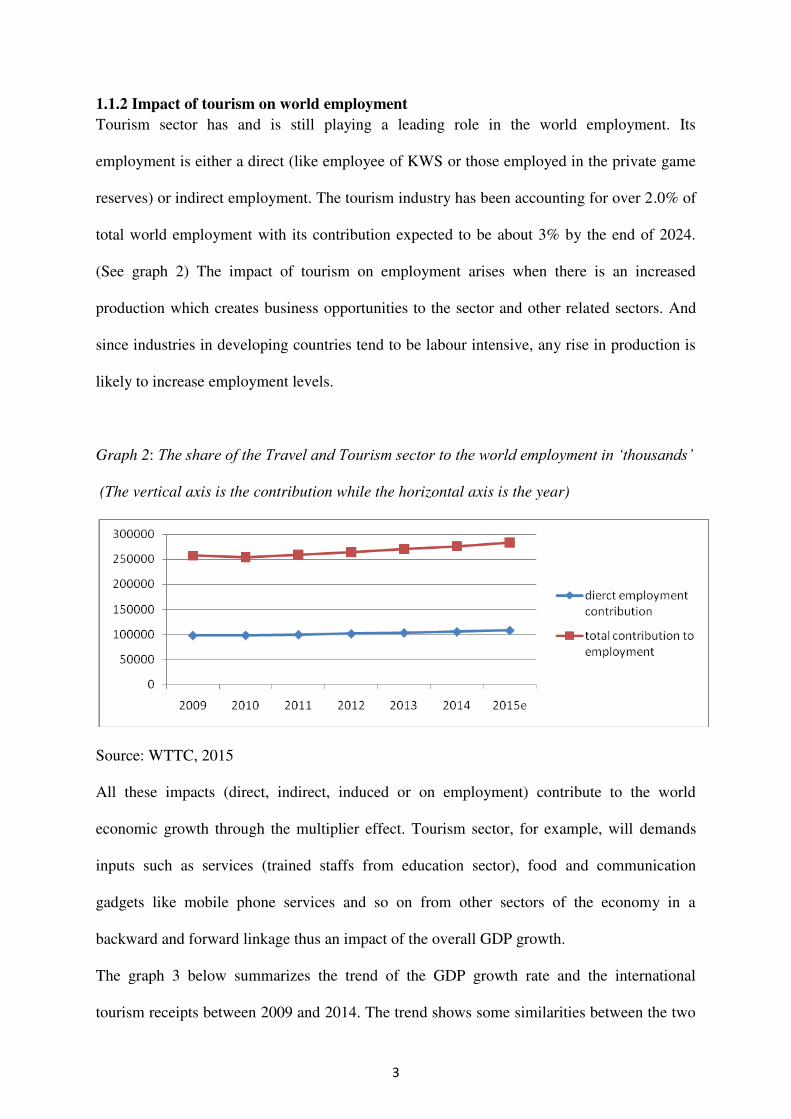
1.1.2 Impact of tourism on world employment

Tourism sector has and is still playing a leading role in the world employment. Its

employment is either a direct (like employee of KWS or those employed in the private game

reserves) or indirect employment. The tourism industry has been accounting for over 2.0% of

total world employment with its contribution expected to be about 3% by the end of 2024.

(See graph 2) The impact of tourism on employment arises when there is an increased

production which creates business opportunities to the sector and other related sectors. And

since industries in developing countries tend to be labour intensive, any rise in production is

likely to increase employment levels.

Graph 2: The share of the Travel and Tourism sector to the world employment in ‘thousands’

(The vertical axis is the contribution while the horizontal axis is the year)

Source: WTTC, 2015

All these impacts (direct, indirect, induced or on employment) contribute to the world

economic growth through the multiplier effect. Tourism sector, for example, will demands

inputs such as services (trained staffs from education sector), food and communication

gadgets like mobile phone services and so on from other sectors of the economy in a

backward and forward linkage thus an impact of the overall GDP growth.

The graph 3 below summarizes the trend of the GDP growth rate and the international

tourism receipts between 2009 and 2014. The trend shows some similarities between the two

4

macroeconomic variables. For instance between 2009 and 2010, both world GDP and

international receipts were rising. The trend also depicts a decline trend after 2010 for both

macroeconomic variables hinting some theoretical relationship.

Graph 3 World GDP growth rate and international receipts growth rate between 2009 and

2014

Source; UNCTAD, 2015

1.1.3 International tourism arrivals.

The international tourism arrival is closely related to the receipts. The arrivals have shown an

upward trend. For instance, the number of international tourist arrival worldwide reached

1138 million in 2014 which was 51 million more than the previous year 2013 (an equivalent

to a 4.7% increase in the two periods). However, there was a slight fall in the number of

international tourist arrival in 2003 and 2009 that has been associated with the financial crisis

in the developed economies especially the United States and Europe. Despite this impressive

rise of the tourism arrivals worldwide, the African economy’s share of the international

tourist arrivals remained dismal throughout the period.

5

1.1.4 Kenyan’s sector performance

In Kenya, tourism sector is a sub pillar in the economic pillar as stated in its vision 2030

which has been charged with the transformation of the country to better nation (Akama,

2000). Tourism is classified as a service sector among others such as social services, private

services, insurance, financial services and so on. Tourism share is captured by restaurants,

hotels and safari industry. There are three main sectors that contribute to the Kenyan GDP:

Agricultural sector, Service sector and the Industrial sector (Mings, 1978). (See the graph 4

below)

Graph 4Kenyan percentage share of GDP by main sector for some selected years

Source: KNBS, 2002

From the graph 4 above, the contribution of the service sector has been rising since 1960

where its share to the Kenyan GDP rose from 44% in 1960 to slightly above 62% in 2000.

Agriculture, which remains the backbone of Kenyan economy, has maintained a downward

trend with it share to the GDP being 38% in 1960 to 20% in 2000. The industrial sector on

the other hand has been fairly stagnant averagely at 19% throughout the last five decades.

Some of the reasons accounting for the dismal performance of the industrial sector have been

6

low level of domestic savings amongst the Kenyan citizens to finance acquisition of capital,

inappropriate technology and high cost of establishing business within the country (Mitchell,

1968).

1.1.5 History of the tourism sector since 1960

Kenyan’s tourism sector performed generally better in the 1960’s mainly due to her rich

endowment of tourist attraction sites or the natural resources as well as human factors such as

development of package tours by Kenyan government and the general hospitality of Kenyans

among other reasons. But in the early 1970’s the sector registered the first decline in the

number of tourist arrival to the country. Economic recession that had hit the traditional home

countries such as United Kingdom and USA were suggested as the possible causes of the

decline (Dieke, 1991). Internal shocks such as the closure of the Kenya-Tanzania border in

1977 and the attempted coup of 1982 did worsen the problem even further leading to a dismal

performance of this sector (Dieke, 1991). Graph 5 below that shows the international tourism

receipt for Kenya between 1995 and 2013

Graph 5.Trend of international tourism receipts to Kenya in thousand US dollars

Source: WDI, 2014

From the graph 5 above, international tourism to Kenya has a double maxima receipt regime

(at 1988 and 2007) with another promising after 2011. These receipts are very important in

7

the economy as they are used to purchase capital goods such as machines for further

production and hence improving the economic performance of the country (Chen and

Devereux, 1999).

The 1990’s witnessed yet another decline. This round it was because of political instigated

shock that was causing unrest ( 1991-1992 saw Kenya adopt multi-party state), sudden rise in

general oil prices as well as widened misleading perception ran by international media houses

about Kenya due to high incidences of insecurity and the spread of STD ( HIV in the

region) Ikiara et al. (1994). Starting 2010, earnings from tourism receipts rose by 18.5%.

This rise in tourism receipt continued all through to 2012 although at a lower percentage of

3.3% as compared to the period 2010-2011(KNBS, 2013).

For Kenya, the direct tourism impact accounted for Ksh. 167.6 billion (about 9.5% of the

GDP) in 2011. Full impact in the same year was estimated to13.7 % of GDP while direct

employment was 8.4% (created over 31300 jobs). Full employment impact stood at 11.9% in

the same year. From the graph 6, it is evident that the impact of travel and tourism was

negative in 2008 and attained its peak in 2010 before it started a declining trend up to 2013

(WTTC, 2015)

Graph 6. The role of Travel and tourism industry to the economic growth of Kenya

Source: WTTC (2015)

8

Despite the rising economic significance of tourism sector to the Kenyan economy, the sector

has attracted very little empirical research (Lanza et al, 2003). Some of the studies in this

area have been mainly focusing on the calculation of the demand of the industry and the gains

generated by the industry either directly or through the multiplier effect (Figini and Vici,

2010). The study fills the gap by analyzing the empirical effect of international tourism

receipts to the Kenyan’s economic growth using a time series data between 1980 and 2013. In

particular, the study tends to answer the question of the causality between the two

macroeconomic variables. The period under study is very unique since Kenya started

experiencing major internal shocks such as attempted coup of 1982; inter clashes due to

multiparty elections of 1991-92, terrorism attack of 1997, post-election violence of 2007/08

as well as political tension associated with 2013 elections. All this shocks affects the tourism

environment by portraying Kenya as a dangerous destination.

1.2 Statement of Research Problem

The Kenyan tourism industry has been singled out as the main sector for realizing the

country’s Vision 2030. It is critical for employment, foreign exchange earnings, foreign

investment and generally economic growth. According to the WTO report (2014), the

country’s share of global tourist arrivals rose from 0.17% in 1980’s to 0.19% in 1990’s. By

2000, Kenya was the 6th most visited nation in Africa after the traditional tourist destinations

such as South Africa, Tunisia, Morocco, Zimbabwe and Botswana in that order. But it lost

the leverage by 2001 when African destinations like Algeria and Nigeria overtook it. Since

then its position as one of the Africans most visited destination has been unstable with

internal shocks like the post-election violence of 2007/2008 as well as the fear from general

elections of 2013 threatening the sector from fully recovering.

9

These facts direct the interest of this study. Kenyan vision 2030 do recognize tourism sector

as one of the sub-pillar in the economic pillar yet very few empirical studies have been done

in Kenya with none focusing on the causality between the economic growth and the

international tourism earning. The study answers this critical linkage by analyzing the time

series data of Kenya between 1980 and 2013 using endogenous growth model and new

econometric techniques such as cointegration and Granger Causality test. Main variables will

be economic growth rate, fixed capital formation, total expenditure on education (as a proxy

of human capital), real exchange rate, share of ICT on exports (as a proxy of level of

technology), GDP per worker, internal shocks and international tourism receipts.

1.3 Study questions

The study intends to answer the following research questions:

I. What is the effect of international tourism receipts on economic growth in Kenya?

II. What causal relationship exists between international tourism receipts and economic

growth in Kenya?

1.4. Study Objectives

1.4.1 The general objective

The overall aim of this study is to analyze the relationship between international tourism

receipts and economic growth in Kenya.

1.4.2 The specific objectives.

1) To estimate the effect of international tourism receipts on economic growth in Kenya

2) To find the causal relationship between the international tourism receipt and

economic growth in Kenya.

3) To offer policy recommendation based on the study findings.

10

1.5 Significance of the study

The sector of tourism has drawn a lot of attention especially in diversification to the

economies of developing nations and small islands are concerned. However, the analysis

techniques employed in the previous studies on real influence of tourism on economic growth

have been inefficient and inadequate application of new developments in econometrics

analysis such as co-integration and Granger causality concepts. Based on these new

econometric techniques, the study outcome will be helpful in three folds: First is to the

economies of developing countries such as Kenya and small Islands that are aiming to either

diversify their economies or industrialize their production process, the policy makers will be

able to formulate informed decisions from the empirical results of this study. Secondly, the

local and international investors involved in tourism supply chain will stands to benefit from

the increased information and lastly it will add to the existing body of literature by using the

Kenyan data which will form the basis for further research.

1.6 Organization of the proposal

Following this introduction is Chapter Two which presents the theoretical literature review as

well as the empirical literature review and the overview of the two. Chapter Three is the

methodology and discusses the conceptual framework, model specification, empirical model,

data type, source and topology of the variables as well as the pre-test statistical tests that is

used to analysis the data. Chapter Four is the analysis of data and discussion of the result. It

thus presents the descriptive statistics, diagnostic tests and the empirical findings. Chapter

Five presents the summary of the study findings, conclusion and policy recommendation. It

begins with the motivation of the study followed by summary findings and policy

11

recommendation and then winds up with the limitations of the results and the areas for further

research.

12

CHAPTER TWO: LITERATURE REVIEW

2.1 Introduction

This chapter presents the theoretical literature review as well as the empirical review of

recent he same area. It then summarizes by discussing the overview of both the theoretical

and empirical review.

In a broad sense, tourism can be classified as mass tourism (usually characterized by short

term gains but with high density development) or alternative tourism which is characterized

by consumption of locally produced goods and services (Weaver, 1999, Woodside and

Lysonski, 1989). Therefore alternative tourism has been closely associated with ecotourism

and sustainable tourism according to WTO standards.

2.2 Theoretical literature review:

Keynesian model of an open economy

To develop our theoretical literature, assume two identical nations (Nation X and Nation Y).

Let the only difference between the two nations be nation X receives tourist inflow while

nation Y does not. If we considering an open market economy by the Keynesian school of

thought, then a consumption of services and goods (through increased aggregate demand) in

nation X by the foreign tourists will stimulate the production of more goods and services as

well as income to the sector. And since, according to Eugenio-Martin & Morales (2004),

tourism tends to be more of labour intensive then a rise in production is closely associated

with a rise in employment. They farther suggest that the increase in employment is crucial to

developing countries whose production is still below the full employment level. They

however warn that the high demand for employment may raise wages which may create a

shock in the job market inducing mobility across the sectors- what macroeconomist may term

as the Dutch diseases that may greatly affect the lagging sector of the economy.

13

Sinclair (1998) is of the idea that the economic influence the tourism sector on any nation’s

economic growth should be examined in two folds: that is the positive influence and the

negative influence on the society. The positive influences revolves around the provision of

hard currency that is very crucial in the purchases of capital goods, increased personal

income, raises the tax revenue base as well as additional employment opportunities.

Expenditure by foreign tourist may lead to accumulation of physical capital mainly due to

domestic tourism constructions as well as human capital development as the sector demand

for skilled labour. Negative impacts may arise, according to Hazari and Ng (1993), when

tourists spends on internally produced products thus affecting both the tertiary and non-

durable goods consumption sector. To them, a rise in demand of locally produced goods and

services due to demand from the foreign tourist, reduces the resident’s welfare as real wages

are affected by the demand cause inflation. However they are optimistic that this negative

impact is sometimes compensated by the positive/constructive effect on the overall welfare of

the country. Gursoy & Rutherford (2004) summarizes the negative influences of tourism as

rising pollution, traffic jams, degradation of the environment, emergency of crime as well as

violence related to tourism. The host country has therefore to spend a lot of resources in

improving the domestic security. The net effect is a reduction in the net benefit from the

tourism industry.

2.2.1 The theory of tourism consumption system

According to this theory, the influence of one tourism activity influences the decisions of a

potential tourist on subsequent activities. This theory therefore narrowly puts a prediction

behavioral pattern which should be observable in the consumption of the tourist products

(Woodside and Roberta, 1994). The theory goes on to highlight some of the main variables

14

that can be used to explain the choice of destination like the marketing strategy by the host

country and present/current trip planning by the tourist (Woodside and Roberta, 1994).

However, many scholars have criticized the inability of this theory to predict and explain the

choice of the tourist destination.

2.2.2 Tourism-Led Growth Hypothesis (TLGH)

This is a hypothesis that stipulates that an economy’s growth can be raised not just by adding

more labour units and/or capital units in the production process but also through expanding

export (Balassa, 1978). While using the endogenous growth model developed by Lucas

(1988), Pigliaru&Lanza (1995) compares two nations. One nation’s economy specializing in

the manufacturing/ processing of goods while the other economy specializing in production

of tourism goods in order to find out whether or not tourism sector leads to a lower economic

growth than manufacturing of goods. Their main assumption was that while the

manufacturing of goods benefited from technological progress, tourism industry lacked this

crucial technological advantage. They concluded that tourism industry would grow much

faster than the manufacturing sector if and only if the two goods or product in question were

not close substitute and an increase in the TOT was higher than the compensation of the gap

in technologic between the manufacturing sector and tourism sector. Candela and Cellini

(1997) later showed that the technological gap is usually smaller than the terms of trade in the

case of a small economy (smaller by size). Small economies were found to posses smaller

opportunity cost to specialize in tourism which is a good opportunity to developing nations

such as Kenya.

2.3 Empirical literature review

This part reviews some of the recent empirical studies done by other scholars in the area

under study and their findings.

15

Sinclair et al. (2010), in their study of TLGH, found out that tourism sector had a positive

influential role in economic growth through creating employment opportunities and income

generation to the government through foreign exchange earnings to the recipient economy.

The foreign exchange is usually a vital component in economic growth to especially

developing nations as it is used to purchase capital goods for further production and thus

expanding the output of such a recipient nation.

Lean and Tang (2010) investigated the causality among tourism receipts and gross domestic

product of Malaysia in the period 1989 - 2009 by a VAR (which suffers spurious regression

problem in case the data is non-stationary). The study revealed a causality running from the

receipts to economic growth for the country.

While investigating the causality between international tourism receipts and economic growth

in Greece using a VECM for the time period between 1960 and 2007, (Kasimati, 2011) found

out that the causality ran in both sides (bidirectional causality). This meant that previous

year’s tourism receipts could be used to explain the economic growth of preceding year and

vice versa.

Same study was carried on by Belloumi (2010) using Tunisia data of between 1970 and 2007

and applied a VECM and he found that the causality was bidirectional meaning tourism could

be used to explain the variation in economic growth and equally economic growth could

account for the variation in tourism sector.

Another study in Turkey by Zortuk (2009) investigating the relationship between economic

growth and tourism growth found out a unidirectional causality running from international

16

tourism receipts to Turkey’s economic growth. His time period was however less than the

minimum thirty years required in a time series data since it was between 1992 and 2008. This

study was improved by Katircioglu (2009) who applied VECM on Turkey on a larger data for

a 46 year period. The study findings reveal no causality between the two macro economic

variables. However, Arslanturk et al. (2011) used data from 1963- 2006 from the same

country to show an existence of a unidirectional causality running form the receipts to

economic growth by applying rolling window and time-varying coefficients estimation

methods.

On studying the contribution of tourism earnings on gross value addition, Odunga and Folmer

(2004) used a seven-year data from 1995 and 2001 and found out that tourism contributed to

an approximately twelve-percent of gross domestic product in this period. They also found an

existence of bidirectional causality between the two macroeconomic variables.

Lee & Chang (2008) studied the influence of tourism sector on the economies of both OECD

and Non-OECD countries using a panel data for twelve year period. Their result reveals a

contrary for the two regions. The results were interesting with a revelation of unidirectional

and bidirectional causality in OECD and Non-OECD respectively.

In their study of cointegration and causality between tourism growth and Taiwan’s economic

development, Kim et al. (2006) applies Cointegration and Granger causality tests. The study

revealed that all variable used were cointegrated and finds Granger causality test was

bidirectional causality.

17

Using Korean data to find causality between economic growth and tourism expansion, Oh

(2005), applies Engle-Granger two stage methods and VAR model. Although he found no

existence of long-run equilibrium between tourism growth and economic growth, his results

found out a unidirectional relationship between economic growth and tourism growth for

Korea.

Brida, et al, (2008b) studied data from Mexico to establish causality for three macroeconomic

involving current account, economic growth and tourism expenditures for the period 1980 to

2007. They found out a unidirectional relationship running from tourism expenditure to real

gross domestic product.

According to Tonamy and Swinscoe (2000), the impact of tourism on employment can either

be direct and indirect. The direct tourism jobs constitute approximately 5.7% of national

employment in Egypt while the indirect and induced jobs included are about 12.6%. They

further suggest that Tourism account for over 10% to Egypt’s GDP. But to Archer and

Fletcher (1996), Tourism expenditure’s Impact varied by the country of origin of the tourists

so that if the tourist originate from a country with a higher spending behavior, there will a

greater economic impact. Their study shows that tourism earning alone accounts for over

24% of GDP in Seychelles.

Durbarry (2004) while investigating the practicability of the Tourism-led growth hypothesis

using an endogenous growth model that assumed economic growth as a function of in three

variables (physical capital, human capita and tourism receipts), used value of exports to

proxy international tourism receipts. The study found a bi-directional causality. Our study

completes this study by using the international tourism receipts data to test for the causality

between the two macroeconomic variables.

18

2.4 Overview of the literature

Most theoretical and empirical literature review (above) supports an existence of a positive

and significant influence of international tourism receipts on economic growth of a nation.

While some studies such as Archer and Flestcher (1996) have found a positive impact of

international tourism receipts on economic growth, others such as Hazari and Ng (1993) have

warned of a possible negative influence resulting from insecurity brought by tourism

activities. For causality between the two macroeconomic variables, studies are dividing with

some finding a unidirectional causality like Lean & Tang (2010) while other finding a

bidirectional result like Kasimati (2011) and Belloumi (2010). However none of these studies

have been done in Kenya. This study therefore bridges the knowledge gap by extending the

study to Kenya.

19

CHAPTER THREE: METHODOLOGY

3.1 Introduction

This section presents the methodology of the study and thus discusses the conceptual

framework, the theoretical framework, empirical model and the pre test estimations.

3.2 Conceptual framework

There exist a powerful linkage between receipts from cross-border tourism and some key

economic sectors of the economy. For instance visitor’s arrival has a multiplier effect on the

economy where expenditure rise increasing the revenue of both the government and the

private firms associated with the tourism activities (Marin (1992). From the figure below, it’s

clear that the influence of the tourism sector is in three folds: through direct impact (that

involves expenditures by tourist within the tourism sector on the typical tourism products),

through the indirect impact (that entails consumption of all intermediate goods by the tourism

sectors such as goods that they buy from their suppliers. Usually forms the tourism supply

chain and crucial for the promotion of locally produced goods) or through induced impact

(that includes expenditures by employees of the tourism sector or companies that benefit

from tourism on locally produced goods and services).

20

3.3 Theoretical frameworks

Many different models have been used to study the influence of tourism industry on country’s

economic performance. While some have tried to incorporate the tourism demand on the

aggregate domestic demand ( Hazari et al, 1995), others have applied the growth model

(Durbarry, 2004).For instance, (Durbarry, 2004) model assumes that economic growth is a

function of three variables 𝑌𝑡 = 𝑓(𝑃ℎ𝑦𝐾𝑡, 𝐻𝑢𝑀𝑘𝑡 , 𝑒𝑥𝑃𝑡) … … … … … … … … .1

Where 𝑃ℎ𝑦𝐾𝑡is the Physical capital in period t 𝐻𝑢𝑀𝑘𝑡is the human capital in period t 𝑒𝑥𝑃𝑡is the total exports of a nation at period t

Our study extends the endogenous growth model adopted by Durbarry (2004) and contributes

to the existing literature through extending the study to the Kenya case as follows

DIRECT IMPACT

(Expenditure by tourist within

the tourism sector such as

buying of typical tourism

products, paying for entry fees

etc.)

INDIRECT IMPACT

(Includes all intermediate

goods produced locally

and used by the tourism

sector. Such goods are

obtained from suppliers

of the tourism sector)

INDUCED IMPACT

(This includes all expenditures by

tourism employees on the local

economy. May include the

expenditures of all companies

paid by the tourism sector on

the local economy

Economic

growth

21

𝑌𝑡 = 𝑓(𝑃ℎ𝑦𝐾𝑡 , 𝐸𝑑𝑢𝐸𝑥𝑝𝑡 , 𝐼𝑛𝑡. 𝑇𝑅𝑡, 𝐸𝑋𝑅𝑡, 𝑆ℎ. 𝐼𝐶𝑇𝑡, 𝑇𝑟𝑑. 𝑂𝑃𝑛𝐾𝑡, 𝐷𝐵𝑡. 𝐵𝑑𝐾𝑡, 𝐺𝐷𝑃/𝑊𝑜𝑟𝑘𝑒𝑟𝑡, 𝑀2/𝐺𝐷𝑃𝑡 , 𝐼𝑛𝑡. 𝑠ℎ𝑜𝑐𝐾𝑡)…………………………………………..2

Where: 𝒀𝒕= Gross Domestic Product growth rate representing the economic growth of Kenya at

period t 𝑬𝒅𝒖𝑬𝒙𝒑𝒕 = total expenditure in education and a proxy of the human capital and labour

productivity of the country measured in US Dollars at period t 𝑷𝒉𝒚𝑲𝒕= country’s Gross fixed capital formation in periodt 𝑬𝑿𝑹𝒕= country’s real exchange rate which is a proxy used to measure international

competitiveness 𝑰𝒏𝒕. 𝑻𝑹𝒕= international tourism receipts (US Dollars) and the main variable under study 𝑺𝒉. 𝑰𝑪𝑻𝒕= is the variable used to capture the level of infrastructure. It is the share of ICT as a

percentage of export. Trd. OPnKt= thetrade openness measured as (Exports + imports)/GDP time 100 DBt. BdKt= the debt burden of the country which is the ratio between debt services and

exports time 100 𝑴𝟐/𝑮𝑫𝑷𝒕= the percentage ratio of broad money (M2) and the GDP which is a proxy of the

financial deepening

= the ratio gross domestic product per employed person at constant1990and a

proxy of the average wage

= the internal shocks that have occurred for the past 34 years

3.4 Empirical model

To estimate the theoretical model in equation 1, the study adds an error term that will

capture the characteristics of the statistical nature of the empirical analysis as follows.

22

𝑌𝑡 = 𝑓(𝑃ℎ𝑦𝐾𝑡 + 𝐸𝑑𝑢𝐸𝑥𝑝𝑡 + 𝐼𝑛𝑡. 𝑇𝑅𝑡 + 𝐸𝑋𝑅𝑡 + 𝑆ℎ. 𝐼𝐶𝑇𝑡 + 𝑇𝑟𝑑. 𝑂𝑃𝑛𝐾𝑡 + 𝐷𝐵𝑡. 𝐵𝑑𝐾𝑡 +𝐺𝐷𝑃/𝑊𝑜𝑟𝑘𝑒𝑟𝑡 + 𝑀2/𝐺𝐷𝑃𝑡 + 𝐼𝑛𝑡. 𝑠ℎ𝑜𝑐𝐾𝑡 +∈𝑡…………………………………………..3

Where

α0 = the intercept

α1, α2, …, α5 are the unknown slope coefficients for the exogenous variables in the model ∈t = the term that captures error in measurements or variables not included in the model.

The subscript t captures the time period.

3.5 Data type, source and Typology of variables

This study will be based on the annual time series data (1980-2013) of the macroeconomic

variables GDP growth rate, physical capital accumulation, overall expenditure on education,

share of ICT on exports (as a proxy of the level of infrastructure), trade openness of the

country, GDP per worker (as a proxy of the average wage), the percentage ratio of M2 to

GDP (as a proxy of the financial deepening), internal shocks, the country’s competitive

advantage (represented by real exchange rate) and international tourism receipts. It utilizes

secondary data from World Bank Indicators (WDI), International Labour Organization (ILO),

various government documents and UNCTAD database.

Table 1.Shows the type of data, source &Typology of variables

Variable name Variable

proxy

Description Expected

sign

Source

Economic

growth

Yt Real GDP growth rate

expressed in percentage

Is the

dependent

variable

UNCTAD

2015

Human capital

accumulation

𝐸𝑑𝑢𝐸𝑥𝑝𝑡 Total expenditure on

Education in US Dollars

inconclusive WDI (2015)

23

Variable name Variable

proxy

Description Expected

sign

Source

International

competitiveness

𝐸𝑋𝑅𝑡 Real exchange rate of Kenya -/+ WDI (2015)

Gross fixed

capital

formation

𝑃ℎ𝑦𝐾𝑡 Gross fixed capital formation

in US Dollars

+ WDI (2015)

International

Tourism receipt

𝐼𝑛𝑡. 𝑇𝑅𝑡 International Tourism receipt

in US Dollars

+ WDI (2015)

Internal shocks 𝐼𝑛𝑡. 𝑠ℎ𝑜𝑐𝐾𝑡 Dummy variable1=if there

was an shock

0=otherwise

- Various

economic

surveys from

1980 to 2014

Debt burden 𝐷𝐵𝑡. 𝐵𝑑𝐾𝑡 (Debt service÷Exports)x100 - WDI (2015)

Level of

infrastructure

𝑆ℎ. 𝐼𝐶𝑇𝑡 Share of ICT as a percentage

of the exports

+/- WDI (2015)

(2015)

Gross domestic

product per

worker

𝐺𝐷𝑃/𝑊𝑜𝑟𝑘𝑒𝑟𝑡

Average wage +/- WDI (2015)

Trade openness 𝑇𝑟𝑑. 𝑂𝑃𝑛𝐾𝑡

(Exports+imports)÷GDPx100

+ WDI (2015)

Financial

deepening

𝑀2/𝐺𝐷𝑃𝑡 The percentage ratio of M2

and GDP

+ WDI (2015)

3.6. Estimation technique

The study will estimate the influence of exogenous variables on endogenous variable using

the ordinary least squares (OLS) method. The OLS has a unique advantage in this study as it

uses observable sample whose regression equation can be estimated (Hayakwawa et al.,

2008)

24

3.7. Statistical tests

3.7.1. Unit root and stationarity test

The data to be used in the analysis of this research is a macroeconomic time series which,

from a theoretical perspective suffers from non-stationarity (Nelson and Plosser, 1982). It

will be vital to run a stationarity test first before using it since running a regression on a non

stationary data may lead to invalid empirical result and therefore the study will test

stationarity using Augmented Dickey-Fuller (1979, 1981).

3.7.2. Cointegration test

When two or more macroeconomic variables have a long run relationship, we conclude that

those variables are cointegration. Suppose the economic variables in this study have unit root,

then the study will proceed to test for cointergration tests. To test for cointegration, the study

employed Engel-Granger (1987) test. According to Engel-Granger (1987), if the residuals

are stationary, then it means that the variables are co-integrated

3.7.3. Vector Error Correction Model

It determines whether the error correcting term has a long run causality effect. It is a special

model in that it ensures that the economic variables in the model are stationary after first

differencing. For its development, the economic variables must have cointergrating vectors

which will be done first in 3.7.2 above. This model is vital in checking whether an individual

lagged economic variable has any significant effect on the dependent variable. This will be

carried in this study through all the lagged variables and GDP. The sign of the coefficient of

ECT will guide in the conclusion of the direction of causality

25

3.7.4 Granger Causality

This will be to test for the existence of the short-run causality between macroeconomic

variables under investigation. The test checks whether one time series data could be used to

predict another time series data and therefore will be used in this study to check whether

tourism receipts could be used to forecast the GDP of Kenya in the future. The study will

therefore conduct a check on whether the lagged variables combined have any significant

influence on the depended variable. It will also be used to determine the type of causality

between GDP and tourism receipts.

3.7.5 Diagnostics Tests for Normality and Serial Correlation

This study will utilize Shapiro-Wilk test to conduct a normality test for the error term. It will

involve computation of the, W, V, Z and P-value. We use the p-value to make an inference of

normality. If our calculated p-value exceeds the critical value, then the variable will be

statistically significant or normal in our case. If the calculated p-value is smaller than the

critical value, then a variable is not significant or not normal. The credibility of the OLS

parameters will be test through testing for the degree of multicollinearity and

heteroscedasiticity.

26

CHAPTER FOUR: ANALYSIS OF DATA AND DISCUSSION OF RESULTS

4.0 Introduction

The section presents the study results from the empirical analysis and discusses their

economic interpretation. It begins with the description of all variables used in our model

followed by diagnostic tests of a time series data and finally an OLS regression and a

discussion of results.

4.1 Descriptive statistics

Descriptive statistics was mainly carried out in this study to ascertain the statistical

characteristics of the data used in the model. This study uses annual time-series data between

1980 and 2013. The main variables under study include GDP growth rate and the receipts

from international tourism (indicating the performance of the tourism sector) while other

variables like total expenditure in education, gross fixed capital formation, real exchange rate

(an indication of the international competitiveness), share of ICT on exports, trade openness,

debt burden, GDP per worker (a proxy of the average wage) ,the ratio of M2 and GDP

(proxy of financial deepening) and internal shocks acted as control variables. Most variables

were obtained from the world development indicator (WDI, 2015) while some were from the

UNCTAD (2015) online website.

27

Table 2: shows the descriptive statistics

Variables

name

Mean of

variable

Standard

Dev.

Maximu

m

Minimu

m

Kurtosis

Skewnes

s

Yt 3.680969 2.3232 -.793179 7.71446 2.087698 -

.3046491 𝑃ℎ𝑦𝐾𝑡 18.41025 .3006374 21.38559 15.3879 -.1554632 1.911264 𝐼𝑛𝑡. 𝑇𝑅𝑡 797000000 96500000 2000000

0

4000000 1.80325 .4808693

𝐸𝑑𝑢𝐸𝑥𝑝𝑡. 6.001101 1.253328 4.58096 7.33565 1.773207 .1525013 𝐸𝑋𝑅𝑡 51.13586 28.05369 7.568 88.72775 1.458144 -

.3066223 𝐼𝑛𝑡. 𝑠ℎ𝑜𝑐𝐾𝑡 .3235294 .4748581 0 1 1.56917 .7544335 𝑆ℎ. 𝐼𝐶𝑇𝑡 13.8537 19.19557 1.300369 70.04114 4.291739 1.655703 𝑇𝑟𝑑. 𝑂𝑃𝑛𝐾𝑡 14.70059 5.112746 9.62 27.47 3.74718 1.342622 𝐷𝐵𝑡. 𝐵𝑑𝐾𝑡 2798.476 1427.666 690.62 5270.46 1.853548 -

.0464977 𝐺𝐷𝑃/𝑊𝑜𝑟𝑘𝑒𝑟𝑡

3046.206 224.5863 2689 3448 1.973461 .0245852

𝑀2/𝐺𝐷𝑃𝑡 34.81621 4.580551 26.68185 42.23227 1.747896 -

.1961378

Source: Author’s calculation

From table 2 above, the GDP growth rate has a mean of 3.68% with a standard deviation of

2.32% and a respective minimum and maximum of -0.793% and 7.71%. The average gross

fixed capital formation within the 34 year period is 3511.643 million US dollars with a

28

standard deviation of 2751.722 million US dollars. The highest gross fixed capital formation

is 11276.95million US dollars and the lowest is 1199.945million US dollars. The mean of

international tourism receipts in US dollars is 647 million with a standard deviation of

671million and a minimum and maximum of 331740Us dollars and 200million US dollars

respectively. The international tourism receipts have steadily increased since 1980. The

average expenditure on education is 6.0 percent of total government expenditure while the

minimum and maximum expenditure on education is 4.58% and 7.34% of the total

government expenditures respectively. The average real exchange rate (real) is at 51.18824 in

the 34 year period with its standard deviation being 27.98382. The minimum real exchange

rate is at 7.57while maximum exchange rate (real) being 7.57.

Since the study used time series data, Kurtosis and Skewness were employed to give a clue of

the trend of the individual variable. Kurtosis measures the flatness of the distribution and

with the results from the table 2 above; it reveals that all the variables are leptokurtic since

their distributions are peaked sharper than a normal distribution. Skewness, which shows the

symmetry of the distribution around the mean of each variable, shows that gross fixed capital,

International tourism receipts, total expenditure on education, internal shocks, share of ICT,

trade openness and GDP per worker are positively skewed. This means that all these

variables have long right tails. The study also reveals that GDP growth rate; real exchange

rate, the percentage ratio of M2 to GDP and debt burden are negatively skewed, implying that

they have a long left tail.

29

Pre-estimation tests

4.2 Diagnostic tests

4.2.1Normality test

This study uses the Shapiro-Wilk test to determine normality of variables. A variable is

normal if the mean, median and mode are equal (that is normally skewed). The Shapiro-Wilk

test gives four options, a W, V, Z and P-value. We use the p-value to make an inference of

normality. If our calculated p-value exceeds the critical value then our conclusion is that the

variable is normal. But if the calculated p-value is smaller than the critical value, then a

variable will be non-normal.

Table 3: Shapiro-Wilk normality test

Variable observation W V Z Prob>z status

Yt 34 0.96098 1.363 0.645 0.25956 Normal 𝑃ℎ𝑦𝐾𝑡 34 0.73807 9.146 4.612 0.00000 Non-normal 𝐼𝑛𝑡. 𝑇𝑅𝑡 34 0.84420 5.440 3.529 0.00021 Non-normal 𝐸𝑑𝑢𝐸𝑥𝑝𝑡 34 0.67223 11.445 5.079 0.00000 Non-Normal 𝐸𝑋𝑅𝑡 34 0.87774 4.269 3.024 0.00125 Non-normal 𝐼𝑛𝑡. 𝑠ℎ𝑜𝑐𝐾𝑡 34 0.95630 1.526 0.881 0.18924 Normal 𝑆ℎ. 𝐼𝐶𝑇𝑡 34 0.66071 11.847 5.151 0.00000 Non-normal 𝑇𝑟𝑑. 𝑂𝑃𝑛𝐾𝑡 34 0.80700 6.739 3.976 0.00004 Non-normal 𝐷𝐵𝑡. 𝐵𝑑𝐾𝑡 34 0.93880 2.137 1.582 0.05678 Normal 𝐺𝐷𝑃/𝑊𝑜𝑟𝑘𝑒𝑟𝑡 34 0.95977 1.405 0.708 0.23945 Normal 𝑀2/𝐺𝐷𝑃𝑡 34 0.92787 2.519 1.925 0.02712 Normal

Source: Author’s computation

Results from table 3 above show that only GDP growth rate, the ratio of M2 to GDP, total

debt services and education expenditure are normal at 5% level of significant while the rest of

the variable are not normal.

30

4.2.2 Multicollinearity

This problem arises when two or more independent variables are strongly related. According

to Gujarati (2012), a correlation of 0.8 and above indicates the possibility of collinearity

between two variables. This study used the Vector Integrating Factor (VIF) and Tolerance

(1/VIF) to test for multicollinearity. The VIF test directs that one first runs a regression

followed by a VIF command in Stata. Then an inference is made based on the magnitude of

the VIF value. If the VIF value is less than 10, then a variable has no multicollinearity.

Conversely, if the VIF is greater than 10, then multicollinearity exists.

Table 4: VIF and Tolerance results

Variable VIF /1VIF Status Yt 5.406 0.042873 no multicollinearity 𝑃ℎ𝑦𝐾𝑡 2.332 0.088582 no multicollinearity 𝐼𝑛𝑡. 𝑇𝑅𝑡 9.99 0.100135 no multicollinearity 𝐸𝑑𝑢𝐸𝑥𝑝𝑡 2.45 0.407365 no multicollinearity 𝐸𝑋𝑅𝑡 1.475 0.067789 no multicollinearity 𝐼𝑛𝑡. 𝑠ℎ𝑜𝑐𝐾𝑡 1.541 0.090973 no multicollinearity 𝑆ℎ. 𝐼𝐶𝑇𝑡 1.09 0.913749 no multicollinearity 𝑇𝑟𝑑. 𝑂𝑃𝑛𝐾𝑡 4.44 0.225052 no multicollinearity 𝐷𝐵𝑡. 𝐵𝑑𝐾𝑡 8.00 0.125005 no multicollinearity 𝐺𝐷𝑃/𝑊𝑜𝑟𝑘𝑒𝑟𝑡 7.07 0.141497 no multicollinearity 𝑀2/𝐺𝐷𝑃𝑡 5.44 0.183797 no multicollinearity

Source: Author’s computation

Results from Table 4 above show that there is absence of multicollinearity among all our

variables because all our VIF values are less than 10.

4.2.3 Stationarity (Unit root test)

The study employs ADF test to test for stationarity in the individual variables. According to

ADF test, a variable is declared stationary when it’s t-calculated is smaller than the t-critical.

Table 5: ADF test results

31

Variable Test Statistic

1% critical

value 5% critical

value

10% critical

value

Nature

Yt -3.744 -3.696 -2.978 -2.620 Stationary 𝑃ℎ𝑦𝐾𝑡 3.881 -3.696 -2.978 -2.620 Non stationary 𝐼𝑛𝑡. 𝑇𝑅𝑡 -0.857 -3.696 -2.978 -2.620 Non stationary 𝐸𝑑𝑢𝐸𝑥𝑝𝑡 -3.565 -3.696 -2.978 -2.620 Non stationary 𝐸𝑋𝑅𝑡 -0.943 -3.696 -2.978 -2.620 Non stationary 𝐼𝑛𝑡. 𝑠ℎ𝑜𝑐𝐾𝑡 -4.930 -3.696 -2.978 -2.620 Stationary 𝑆ℎ. 𝐼𝐶𝑇𝑡 -0.717 -3.696 -2.978 -2.620 Non stationary 𝑇𝑟𝑑. 𝑂𝑃𝑛𝐾𝑡 -2.394 -3.696 -2.978 -2.620 Non stationary 𝐷𝐵𝑡. 𝐵𝑑𝐾𝑡 -1.217 -3.696 -2.978 -2.620 Non stationary 𝐺𝐷𝑃/𝑊𝑜𝑟𝑘𝑒𝑟𝑡

-0.717 -3.696 -2.978 -2.620 Non stationary 𝑀2/𝐺𝐷𝑃𝑡 -1.303 -3.696 -2.978 -2.620 Non stationary

Source: Author’s computation

From table 5, only GDP growth rate and internal shock are stationary because their test

statistics are less than the critical value at levels. On the contrary, real exchange, gross fixed

capital formation, International tourism receipts, the percentage ratio of M2 to GDP, GDP

/worker, debt burden, Share of ICT and education expenditure are non-stationary. These non-

stationary variables require additional attention to determine whether they are co-integrated.

Therefore, taking the first difference gives the results in table 6.

Table 6: ADF test results for differenced variables

Variable Test Statistic

1% critical

value 5% critical

value

10% critical

value

Nature

d_𝑃ℎ𝑦𝐾𝑡 -3.776 -3.702 -2.980 -2.622 Stationary

d_𝐼𝑛𝑡. 𝑇𝑅𝑡 -6.096 -3.702 -2.980 -2.622 Stationary

d_𝐺𝐷𝑃/𝑊𝑜𝑟𝑘𝑒𝑟𝑡

-3.287 -3.702 -2.980 -2.622 Non-

Stationary

d_𝑬𝒅𝒖𝑬𝒙𝒑𝒕 -8.128 -3.702 -2.980 -2.622 Stationary

d_𝐸𝑋𝑅𝑡 -6.160 -3.702 -2.980 -2.622 Stationary 𝑑_𝑆ℎ. 𝐼𝐶𝑇𝑡 -5.533 -3.702 -2.980 -2.622 Stationary

D_𝑇𝑟𝑑. 𝑂𝑃𝑛𝐾𝑡 -6.072 -3.702 -2.980 -2.622 Stationary 𝑀2/𝐺𝐷𝑃𝑡

Source: Author’s computation

32

The table above shows all variables that were non stationary at order zero being stationary at

order one i.e. I (1) except for GDP / worker. Taking the second differencing for GDP/worker

shows that it is stationary at the second difference as shown below

Variable Test Statistic

1% critical

value 5% critical

value

10% critical

value

Nature

DD_𝐺𝐷𝑃/𝑊𝑜𝑟𝑘𝑒𝑟𝑡

-12.193 -3.709 -2.983 -2.623 Stationary

4.2.4 Testing for Cointegration

When variables have a long run equilibrium relationship, we say they are cointegrated. Most

of the time when economic variables are individually non-stationary; it is likely that

cointegration may occur. Cointegration test is normally a pre-test for a time series data which

tries to eliminate spurious regression situations of non stationary data. Thus cointegration

relationship existence implies that the regression of non-stationary series in their levels yield

meaningful and not spurious results. To test for cointegration, the study employed Engel-

Granger (1987) test. According to Engel-Granger (1987), if the residuals are stationary, then

the variables in the model are co integrated.

Table7: Engle-Granger Test for Co integration

Variable t-statistic 1% level 5% level 10% level Nature

Residuals -5.088 -3.702 -2.980 -2.622 Stationary

Source: Author’s computation

From table 7, the t- value of test statistics are smaller than all the critical level and hence we

reject the null hypothesis of no co integration among the variables. This therefore implies that

variables in the model do have a long run equilibrium relationship. This shows that regression

of the non-stationary series in their levels will yield meaningful and not spurious results

33

4.2.5 The Granger causality test

To test for the existence of short run causality between macroeconomic variables used in the

model, we run the granger causality. The test checks whether one time series data could be

used to predict another time series data and therefore it has been used in this study to check

whether international tourism receipts could be used to forecast the GDP growth rate of

Kenya in the future

Table 8: Engle-Granger Test

Variable constants Z P>|z| [95% Conf. Interval]

GDP growth rate to

International tourism

L1 -5.42e-10 -0.36 0.722 -3.53e-09

L2 4.19e-10 0.28 0.782 -2.54e-09

International tourism to

GDP growth rate

L1 4.61e+07 2.29 0.022 6594753

L2 -5.21e+07 -2.45 0.014 -9.38e+07 Interpretation of the result

From the result in table 8 above the p-value of 0.022implies that the coefficient of

international tourism receipts is not zero or rather is statistically significant at 95% level.

This is a clear indication that international tourism receipts of the previous year do granger

cause economic growth in the current year. Equally the p-value of 0.722means thatthat the

sample parameter of economic growth rate is not statistically significant- a clear indication

that economic growth rate of the previous year does not cause any change in the receipts of

international tourism in the current year. This result reveals an one-directional causality

running from international tourism receipts to economic growth

4.3 Empirical Findings

Table 9: long run Regression Results in Level

Variable Coefficient t- Statistic P-values (at 5% levels) sign

Yt

d_𝑃ℎ𝑦𝐾𝑡 .0017614 2.50 0.021 +

d_𝐼𝑛𝑡. 𝑇𝑅𝑡 3.02e-10 0.21 0.839 +

34

d_𝐺𝐷𝑃/𝑊𝑜𝑟𝑘𝑒𝑟𝑡

.0107171 2.84 0.010 +

d_𝐸𝑑𝑢𝐸𝑥𝑝𝑡 .3568107 1.20 0.242 +

d_𝐸𝑋𝑅𝑡 -.0638995 0.81 0.425 - 𝑆ℎ. 𝐼𝐶𝑇𝑡 -.0404368 -0.99 0.332 -

d_𝑇𝑟𝑑. 𝑂𝑃𝑛𝐾𝑡 -.0498733 -0.40 0.690 -

d_𝐷𝐵𝑡. 𝐵𝑑𝐾𝑡 -.0006975 -1.28 0.213 - 𝑀2/𝐺𝐷𝑃𝑡 -.1394836 -0.99 0.334 - 𝐼𝑛𝑡. 𝑠ℎ𝑜𝑐𝐾𝑡 -.6345239 -0.91 0.373 -

_cons 3.440495 6.84 0.000

Number of obs = 32

F( 10, 21) = 4.09

Prob > F = 0.0031

R-squared = 0.6610

Adj R-squared = 0.4995

Root MSE = 1.6776

Source: Author’s computation

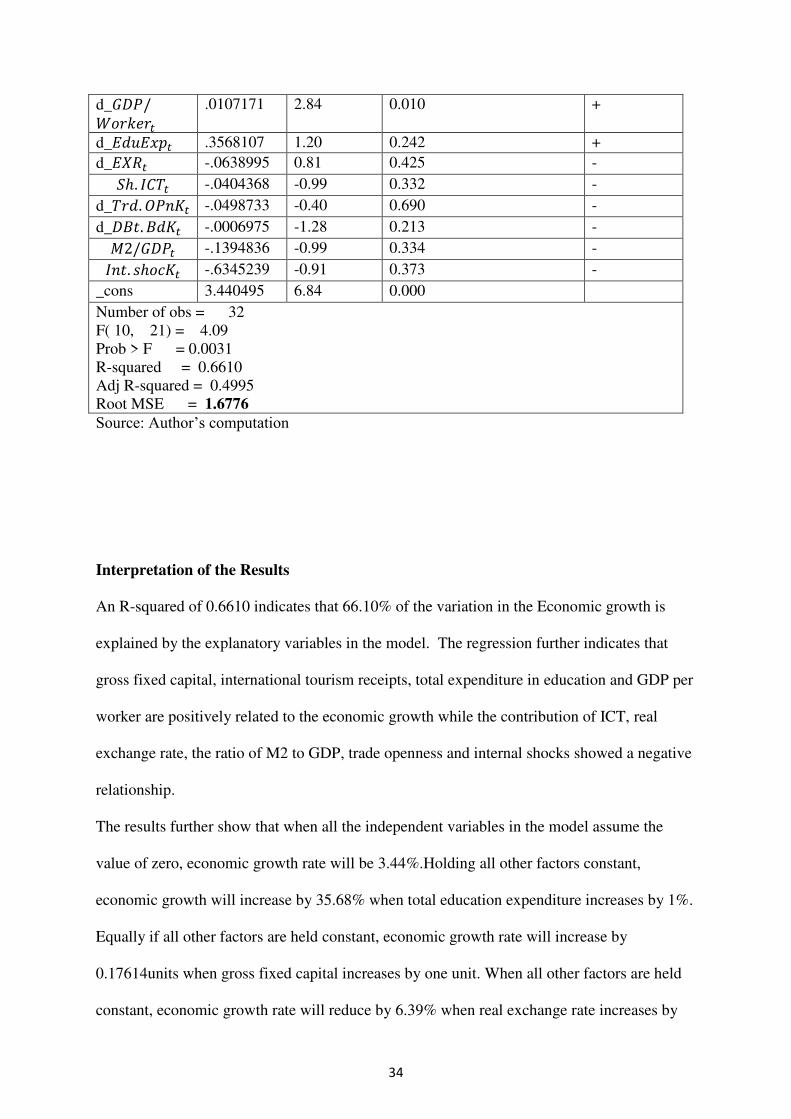
Interpretation of the Results

An R-squared of 0.6610 indicates that 66.10% of the variation in the Economic growth is

explained by the explanatory variables in the model. The regression further indicates that

gross fixed capital, international tourism receipts, total expenditure in education and GDP per

worker are positively related to the economic growth while the contribution of ICT, real

exchange rate, the ratio of M2 to GDP, trade openness and internal shocks showed a negative

relationship.

The results further show that when all the independent variables in the model assume the

value of zero, economic growth rate will be 3.44%.Holding all other factors constant,

economic growth will increase by 35.68% when total education expenditure increases by 1%.

Equally if all other factors are held constant, economic growth rate will increase by

0.17614units when gross fixed capital increases by one unit. When all other factors are held

constant, economic growth rate will reduce by 6.39% when real exchange rate increases by

35

1%. The result also reveals that holding other factors constant, an increase of the share of ICT

in export leads to a 4.04% drop in the economic growth. Equally, a rise in debt burden by one

unit will result to a drop of 0.007 units in the economic growth holding all other factors while

a rise of 1 unit in GDP per worker would result to 1.07%increase in economic growth.

Finally, when all other factors are held constant, economic growth rate will increase by

0.0000003 units when international tourism receipts increases by one unit

4.3.1 Discussion of the results

The coefficient of real exchange rate is positive and insignificant in determining economic

growth in Kenya in the period under study. The results confirm with economic theory since

when real exchange rate increases (what is commonly called devaluation of domestic

currency), imports becomes expensive while exports becomes cheaper in the eyes of

foreigners. Thus the net export should increase thus increasing the economic growth. These

results are also in agreement with Bailey et al. (1986) study which found a positive

relationship between exchange rate and economic growth through increasing of agricultural

exports. However, the results contradict Collins(1997) and Hilton (1984).

The coefficient of expenditure in education is positive and insignificant in determining

economic growth in Kenya. The results conform to economic theory since education

improves labour productivity by equipping workers with information and technology. The

insignificance means that an increase in education expenditure may lead to un-meaningful

result on economic growth. These results are also in agreement with Spence (1973) who

found that education cost was not a good measure of productivity. On contrary, the result

contradicts Mankiw et al. (1992) who found out accumulation of human capital through

education significant to economic growth. His study took into consideration different

36

disciplines where more expenditure on engineering subject lead to an improvement in

economic growth while more expenditure in courses such as law had no significant to

economic growth.

The coefficient of gross fixed capital formation is positive and significant in determining

economic growth in Kenya. The results conform to economic theory since gross fixed capital

formation improves capital productivity and thus improving the economic growth. The result

is in agreement with a study carried by Ku &Pravakar, (2010), Bakare (2011) and Orji, &

Mba, (2010)

The coefficient of share of ICT on exports is negative and insignificant in determining the

Kenyan economic growth within the study period. This study contradicts economic theory

since ICT is a technology which should improves the productivity of labour (Solow,

1956).The negative coefficient may imply that Kenya spends more in the buying of such

technology than what their real contribution to output. Most of the production with the

country is still labour intensive.

The coefficient of trade openness is negative and insignificant in determining the economic

growth in Kenya. This may imply that the country has more restrictions to external trade

through measures such as tariffs and non tariffs. Our study contradict theory that suggest that

a country with higher trade openness and exporting high quality products will grow faster- a

concept the classical economist such as Adam Smith and David Ricardo were advocating

through suggesting the adoption of lazier-fair.

37

The coefficient of debt burden is negative and insignificant at 5% level of significant in

determining the economic growth within the period under study. This confirms with theory

which suggest that at high indebtedness, economic growth will be negatively generated as

government may resort to fiscal policies such as high taxation to repay the tax. Such policies

reduce the money in circulation and reduce disposable income thus reducing the aggregate

demand. The ultimate effect is the reduction in economic growth.

The coefficient of the percentage ratio of M2 to GDP (a proxy of the financial deepening) is

negative and insignificant. This contradicts theory since higher financial deepening are

associate with an expansionary monetary policy which may lead to inflation that encourages

more production in the short run. However, higher inflation may lead low output in the long

run as the real wages are affected leading to a reduction in man hour by the workers.

Although our study contradicted the theory, the coefficient is found to be insignificant.

The coefficient of GDP per worker as a measure of average wage and is found to be positive

and significant. This contradicts theory since average was is a cost in production and should

have a negative effect on economic growth. Although higher wages may motivate the

workers to produce more, its cost implication is negative to growth. The international shocks

are found to have a negative coefficient but insignificant. This conforms to theory as internal

shocks may hinder economic growth.

Finally the coefficient of international tourism receipts is positive and insignificant in

determining economic growth in Kenya. The results conform to economic theory since

expenditures by tourist increases the aggregate demand in the economy leading to increase in

production. Equally an increase of sale of domestic product to the international tourist earns

foreign exchange that is crucial in the importation of capital goods. The result agrees with

38

Katircioglu (2009) who found that international tourism had no significant impact on

economic growth. The study contradicts studies by Arslanturk et al. (2011), Lee and Chang

(2008) and Kasimati (2011) who had found a significant impact of tourism receipts on

economic growth. This could be because tourism industry in Kenya is mostly owned and ran

by foreign investors who repatriate profit to their home country leaving little for the Kenyan

economy.

In the long run, all variable were cointergrated implying that they have a long run relationship

with economic growth. The study therefore conclude that over the period under which the

study has been undertaken, the key determinant of Economic growth in Kenya in the long run

is GDP per worker.

4.3.2The short run regression

Table 10: Regression Results in First Difference

Variable Coefficient

t- Statistic P-values (at 5% levels) sign

Yt

d_𝑃ℎ𝑦𝐾𝑡 .0022397 2.96 0.007 +

d_𝐺𝐷𝑃/𝑊𝑜𝑟𝑘𝑒𝑟𝑡 .0247356 9.04 0.000 +

d_𝐼𝑛𝑡. 𝑇𝑅𝑡 -3.25e-10 -0.21 0.838 -

d_𝐸𝑑𝑢𝐸𝑥𝑝𝑡 .465597 1.44 0.163 +

d_𝐸𝑋𝑅𝑡 .1036226 -1.21 0.236 +

d_𝑆ℎ. 𝐼𝐶𝑇𝑡 -.0641042 -1.44 0.162 -

d_𝑇𝑟𝑑. 𝑂𝑃𝑛𝐾𝑡 .0574952 0.45 0.654 +

d_𝐷𝐵𝑡. 𝐵𝑑𝐾𝑡 -.0005725 -1.00 0.329 - 𝑑_𝑀2/𝐺𝐷𝑃𝑡 -.1548187 -1.01 0.324 -

_cons 3.304004 6.91 0.000

39

Number of obs = 33

F( 8, 24) = 3.20

Prob > F = 0.0128

R-squared = 0.5162

Adj R-squared = 0.3550

Root MSE = 1.8747

Source: Author’s computation

Discussions

The short run regression did not perform different in terms of goodness of fit with an R2 of

0.5162. This implies that 51.62% of the changes in the Economic growth are accounted for

by the exogenous variables in our model. As the result in the diagnostic tests have shown,

autocorrelation and multi-collinearity were all absent. Some of the variables were non-

stationary but were differenced once to become stationary (with GDP per worker being

differenced twice). The short term dynamic allowed us to make some meaningful

interpretation of the dynamic process. One of the variables as depicted in table 10 above is

statistically significant. Thus with such results, the study can discuss the issue of concern.

International tourism receipts remained positive and non significant although it did well in

the short run regression. The only variables that were found to determine the economic

growth in the period under study was gross domestic product per worker and gross fixed

capital formation.

40

CHAPTER FIVE:

5.0 SUMMARY, CONCLUSIONS AND POLICY IMPLICATIONS

5.1 Motivation of the study

The success of any strategic plan of any nation lies behind the practicability of such plans.

Kenya as a nation has given much attention to the tourism sector in its vision 2030. However,

little empirical studies exist in Kenya to help policy planners make informed policies that will

see the vision 2030 a reality. Driven by this lack of information linking international tourism

receipts and economic growth, this study intended to investigate the causality between the

two macroeconomic variables for a period of 34 years

5.2 Summary

This study aimed at analyzing the influence of international tourism receipts on Kenyan’s

economic growth for the period 1980 - 2013 (chosen mainly because of the various internal

and external shocks that have affected the tourism sector such shocks terrorist attacks of

1997, attempted coup of 1982, post election violence of 2007/08). The study sought

specifically to investigate the effect of the receipts from international tourism on the

country’s economic growth as well as the causality between the two macroeconomic

variables. The study obtained its objectives by first identifying cointegration causality test-

for the long term causality followed by Engel-Granger (1987) - for the short term (run)

causality between international receipts from tourism sector and the country’s economic

growth. Results from cointergation test revealed an existence of the long term relationship of

all the variables used in the model while the short term relationship reveals an existence of a

unidirectional causality running form international receipts for tourism to Kenyan’s economic

growth under the time duration of the study. The second objective of our study attempted to

investigate the influence of international tourism on economic growth and was achieved

through regressing the first differencing (short run regression). From the result, despite our

41

main variable under study (international tourism receipts) remained statistically non-

significant in all levels, the result proved that the main determinants for Kenyan economic

growth under the period of study was GDP per worker and gross fixed capital formation.

5.3 Policy implication

Both regression (at long run and short run ), study’s main variable under study (international

tourism receipts) is insignificant. This means that the Kenya as the destination country do

receive very little benefits from tourism sector despite the role it has been assigned to in

achieving vision 2030. There is therefore a need for the government intervention into the

sector through relevant policies such as strengthening the tax body on all foreign companies

dealing with tourism activities within the country, investing more funds to the industry

through improving infrastructure to the attraction sites as well as incorporating the

communities around the attraction sites as tour guides. This will empower such communities

through increased wages and thus raising the aggregate demand to the country. Holding other

factors constant and increase in aggregated demand will boost output thus increasing

economic growth.

Since the study found the causality running from international receipts for tourism to

Kenyan’s economic growth (unidirectional), this justifies the need for the Kenyan

government to boost the tourism sector through advertisement and marketing to areas of the

world where our tourism product are less known since its contribution leads to economic

growth.

The government should also develop policies that will take care of the volatile exchange rate

for example through encouraging flexible exchange rate regime since it was found to be

42

significant in the short run. For the expenditure in education as a proxy of labour

productivity, certain courses like engineering have been found to have a significant role in

labour output compared to say law. It is thus crucial for the government to increase funds for

such disciplines like engineering but reduce expenditure on discipline that have little impact

to the economy. Finally, the government should increase funding to the physical capital

accumulation through encouraging saving in the country since it is significant in the short run

and also positive.

5.2 Limitations of the study

There several control variable that determine economic growth that were not included in the

study since their data was either not enough or was totally missing. Such variables like life

expectancy, fertility rate and inflation among other were we unavailable in the period of

study. Some were very scant and this led to R2 of 66 %. These are important variables that

should have been included in the study but were left out. The study relied mostly on data

available from in WDI and UNCTAD for consistency.

5.3 Areas for further research

The tourism industry is one of the service export sector that can be used to alleviate poverty

in some region in Kenya such as the coastal counties. There is a need for further research on

the impact of tourism industry and the reduction in poverty levels especially where the locals

are given an opportunity to be stakeholders in the sector. There has been an increasing

concern from the wildlife-people conflict just because they don’t feel the gains from the

sector and thus by involving them, they may benefit from the positive spillovers from the

sector.

43

REFERENCES

Archer, B. & Fletcher, J. (1996), ‘The Economic Impact of Tourism in the Seychelles. Annals

of Tourism Research, 23(1): 32-47.

Africa Watch. (1993). Divide and rule: State sponsored violence in Kenya. London,

Washington, New York: Human Rights Watch

Akama, J. (2000). The efficacy of tourism as a tool for economic development in Kenya. In

A. Bujra (Eds.), Development policy management in Sub-Saharan Africa: Tourism

and African development—Trends and critical issues. DPMN Bulletin, 7(1). Addis

Ababa: Commercial Printing Enterprise

Arrow, J. (1973). Higher education as a filter.Journal of Public Economics. 2(3): 193–216.

Arslanturk, Y., Balcilar, M, and Ozdemir, Z.(2011). Time- varying linkages between tourism

receipts and economic growth in a small open economy. Economic modeling. 28, 664-

671.

Bakare, A. (2011); “A Theoretical Analysis of Capital Formation and Growth in Nigeria” Far

East Journal of Psychology and Business Vol 3 No 1 April 2011

Balaguer, J. &Cantavella-Jorda, M.(2002). Tourism as a long-run economic growth factor:

The Spanish case. Applied Economics. 34: 877–84.

Balassa, B. (1978). Exports and economic growth: Further evidence, Journal of Development

Economics, 5, 181–189.

Belloumi, M. (2010). The relationship between tourism receipts, real effective exchange rate

and economic growth in Tunisia, International Journal of Tourism Research, DOI:

10.1002/jtr.774.

Blake, A., Durbarry, R., Sinclair, T., &Sugiyarto, G. (2001).Modeling tourism and travel

using tourism satellite accounts and tourism policy and forecasting models.Tourism

and Travel Research Institute, Discussion Paper 2001/4.

44

Bowcott, O. (1997). Kenya’s violence hurts tourism. The Guardian, August 26th 1997.

Brida, J., Sanchez, E. and Risso, W. (2008b). Tourism’s Impact on Long-Run Mexican

Economic Growth, Economics Bulletin, 3(21), 1–8.

Candela, G. and Cellini, R.(1997). Countries’ size, consumers’ preferences and specialization

in tourism: a note, RivistaInternazionale di ScienzeEconomiche e Commerciali, 44,

451 457.

Chen, F., Chiou-Wei, Z.(2009). Tourism expansion, tourism uncertainty and economic

growth: new evidence from Taiwan and Korea. Tourism Management 30(6): 812–8.

Chen, L., Devereux, J. (1999). Tourism and welfare in Sub-Saharan Africa: a theoretical

analysis. Journal of African Economies 8 (2): 209–27.

Dieke, P. (1991). Policies for tourism development in Kenya.Annals of Tourism Research 18,

no. 2: 269-294.

Dritsakis, N. (2004). Tourism as a long-run economic growth factor: an empirical

investigation for Greece using causality analysis. Tourism Economics 10: 305–16.

Dunn, H. and Dunn, L. (2002). People and tourism: Issues and attitudes in the Jamaican

hospitality industry. Kingston: Arawak Publications.

Durbarry, R.(2004). Tourism and economic growth: the case of Mauritius. Tourism

Economics 10(4): 389–401.

Eugenio-Martin, Juan L., Noelia M. and RiccardoS (2004). Tourism and Economic Growth

in Latin American Countries: A Panel DataApproach. FEEM Working Paper No.

26.2004.

Fayissa, B., Nsiah, C., Badassa, T. (2008).Impact of tourism on economic growth and

development in Africa.Tourism Economics 14(4): 807–18.

Figini, P., Vici, L. (2010). Tourism and growth in a cross section of countries.Tourism

Economics 16(4): 789–805.

45

Gursoy, D., and Rutherford, D. (2004). Host attitudes toward tourism: An improved structural

model. Annals of Tourism Research, 31(3), 495–516.

Hayakwawa K, Kurozumi E. 2008. The role of “leads” in the dynamic OLS estimation of

cointegrating regression models. Mathematics and Computers in Simulation 79: 555–

60.

Hazari, R. and Ng, A. (1993). An analysis of tourists’ consumption of non-traded goods and

services on the welfare of the domestic consumers.International Review of Economics

and Finance, 2, 3–58.

Hazari, R., &Sgro, M.(1995). Tourism and growth in a dynamic model of trade.Journal of

International Trade & Economic Development 4(2): 243–52.

Hazari, R.&Sgro, M. (2004).Tourism, trade and national welfare. Elsevier Science Published.

Ikiara, K., Nyangena, W. &Muriira, I.(1994). “Service in Kenya.” UNCTAD/ CAOAS

Report

Hilton, N.(1984). Exchange rate volatility and Trade: a literature survey. International journal

of Applied studies. Vol. 3-1

Jin, C. (2011). The effects of tourism on economic growth in Hong Kong.Cornell Hospitality

Quarterly 52(333): 333–40.

Kao, C. (1999). Spurious regression and residual-based tests for cointegration in panel

data.Journal of Econometrics 90: 1–44.

Kasimati E. (2011). Economic impact of tourism on Greece’s economy: cointegration and

causality analysis. International Research Journal of Finance and Economics 79: 79–

85.

Katircioglu S. (2009). Revisiting the tourism-led-growth hypothesis for Turkey using the

bounds test and johansen approach for cointegration.Tourism Management 30: 17–20.

46

Kim, J., Chen, M. & Jang S. (2006). Tourism expansion and economic development: the case

of Taiwan. Tourism Management 27: 925–33.

Kweka, J. (2004), ‘Tourism and the Economy of Tanzania: A CGE Analysis’, Retrieved

March 31, 2015, http://www.csae.ox.ac.uk/conferences/2004-GPRAHDIA/papers/1f-

Kweka-CSAE2004.pdf.

Ku DR, Pravakar S. 2010. Economic growth in India: the role of physical and social

infrastructure. Journal of Economic Policy Reform 13(4): 373–85.

Lanza, A., Temple, P., Urga, G. (2003). The implications of tourism specialization in the

long-run: an econometric analysis for 13 OECD economies. Tourism Management

24(3): 315–21.

Lanza, A. and Pigliaru, F. (1995). Specialization in tourism: the case of small open economy,

in Coccossis, H. and Nijkamp, P. (eds), Sustainable Tourism Development, Avebury,

Aldershort.

Lanza, A. and Pigliaru, F. (2000). Why are tourism countries small and fast-growing?, In

Fossati, A. and Panella, G. (eds), Tourism and Sustainable Economic Development,

Kluwer Academic Publisher,Dordrecht, 57–69.

Lean, H. and Tang, F. (2010). Is the tourism-led growth hypothesis stable for Malaysia? A

note, International Journal of Tourism Research, 12(4), 375–378.

Lee, C., Chang, P. (2008). Tourism development and economic growth: a closer look at

panels. Tourism Management 29: 180–92.

Lucas, R. (1988). On the mechanics of economic development, Journal of Monetary

Economics, 22, 3–42.

Mankiw NG, Romer D, Wei DN. 1992. A contribution of the empirics of economic growth.

Quarterly Journal of Economics 107(2): 407–37.

47

Mings, R. (1978).”The importance of more research on the impacts of tourism.”Annals of

tourism research 5(3):340-341

Mitchell, F.(1968). The cost and benefits of tourism in Kenya. Nairobi: Institute of

Development Studies, University of Nairobi

Odunga, O. &Folmer, H. (2004).Profiling tourists for balanced utilization of tourism-based

resources in Kenya. FEEM Working Paper No. 23.2004.

Oh C. (2005). The contribution of tourism development to economic growth in the Korean

economy.Tourism Management 26: 39–44.

Orji, A. & Mba, P. (2010) “Foreign Private Investment, Capital Formation and Economic

Growth in Nigeria: a two stage least square approach” Journal of Economics and Sustainable Development

Razin, O and Susan, M (1997).Real exchange rate misalignment and growth.Georgetown

university press.

Richter, L. K. 1992. Political instability and tourism in the Third World. In Tourism and less

developed countries, edited by D. Harrison, 35-46.

Solow, M.(1956). A contribution to the theory of economic growth.Quarterly Journal of

Economics and Finance 70(1): 65–94.

Sinclair, M. (1998). Tourism and economic development: A survey. Journal of Development

Studies, 34(5), 1–51

Sinclair, M., Stabler, J. &Papatheodorou A. (2010). The Economics of Tourism, London,

Routledge

Sugiyarto, G., A. Blake, and, M.T. Sinclair (2003), ‘Tourism and Globalization: Economic

Impact in Indonesia’, Annals of Tourism Research, 30(3): 683-701.

Spence M. 1973. Job market signaling.The QuarterlyJournal of Economics 87(3): 355–74.

Solow, R. (1956). A contribution of the theory of economic growth.Quarterly Journal of

Economics. 70. No.1:65-94

48

Summary, R. (1987), ‘Tourism's contribution to the economy of Kenya’, Annals of Tourism

Research, 14(4): 531–540

Syriopoulos, T. (1995).A dynamic model of demand for Mediterraneantourism.International

Review of Applied Economics, 9, 318–336.

Tonamy, S. and Swinscoe, A.(2000). ‘The Economic Impact of Tourism in Egypt’, Working

Paper No.40.

West, G. (1993), ‘Economic Significance of Tourism in Queensland’, Annals of Tourism

Research, 20: 490-504.

Weaver, D. (1999). “Magnitude of ecotourism in Costa Rica and Kenya.”Annals of tourism

Research 26(4):792-816

World Bank (2011), Kenya - Country Brief - World Bank

World Tourism Organisation (2001), ‘The Least Developed Countries and International

Tourism’, in Tourism in the Least Developed Countries, edited by the World Tourism

Organization. Madrid: World Tourism Organization.

World Travel and Travel Council (2011), ‘Kenya Economic Impact Report’, Retrieved

March 28, 2015,http://www.wttc.org/site_media/uploads/downloads/kenya2015_2.pdf.

Wattanakuljarus, A. and Coxhead, I. (2008). ‘Is tourism-based development good for the

poor?: A general equilibrium analysis for Thailand’, Journal of Policy Modeling,

30(6): 929–955.

Woodside, G. &Lysonski, S. (1989). “A General Model of Traveler Destination

Choice.”Journal of Travel Research, 27 (4):8-14.

Woodside G. & Roberta, M. (1994). “A General Systems Framework of Customer Choice

Processes of Tourism Services.”In Spoilt for Choice, edited by R. Gasser and K.

Weiermair.Vienna:Kul -turVerlag, pp. 30-59.

World Bank (2010): ‘Kenya’s Tourism: Polishing the Jewel’, Retrieved March 31, 2015,

49

World Bank (2012). Kenya - Country Brief - World Bank

World Tourism Organization, (2001), ‘The Least Developed Countries and International

Tourism’, in Tourism in the Least Developed Countries, edited by the World Tourism

Organization. Madrid: World Tourism Organization.

World Travel and Travel Council (2012), ‘Kenya Economic Impact Report’, Retrieved

March 28, 2015,http://www.wttc.org/site_media/uploads/downloads/kenya2015_2.pdf.

World Travel and Tourism Council (2012)

World Travel and Tourism Council (2015)

Zortuk, M.(2009). Economic Impact of Tourism on Turkey’s Economy: Evidence from

Cointegration Tests, International Research Journal of Finance and Economics, Issue

25, 231-239.