Introduction to Expectation Maximization

Assembled and extended by Longin Jan LateckiTemple University, latecki@temple.edu

based on slides by

Andrew Blake, Microsoft Research and Bill Freeman, MIT, ICCV 2003

and

Andrew W. Moore, Carnegie Mellon University

Learning and vision: Generative Methods

• Machine learning is an important direction in computer vision.

• Our goal for this class:– Give overviews of useful techniques.– Show how these methods can be used in vision.– Provide references and pointers.

What is the goal of vision?

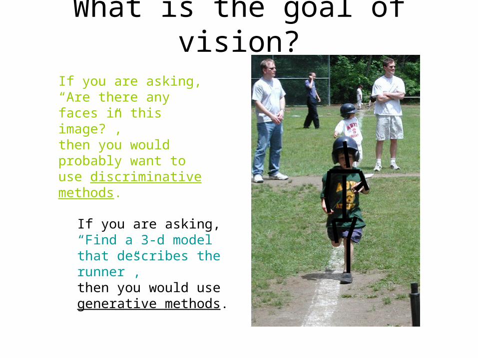
If you are asking,“Are there any faces in this image?”,then you would probably want to use discriminative methods.

What is the goal of vision?

If you are asking,“Are there any faces in this image?”,then you would probably want to use discriminative methods.

If you are asking,“Find a 3-d model that describes the runner”,then you would use generative methods.

Modeling

So we want to look at high-dimensional visual data, and fit models to it; forming summaries of it that let us understand what we see.

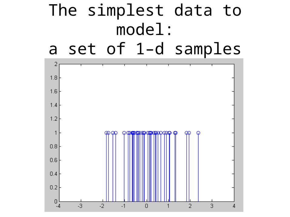
The simplest data to model:a set of 1–d samples

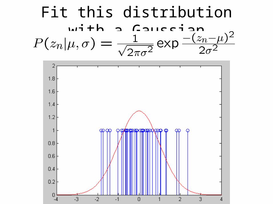
Fit this distribution with a Gaussian

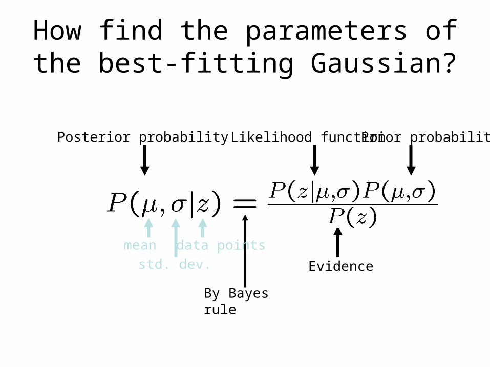
How find the parameters of the best-fitting Gaussian?

Posterior probability Likelihood function Prior probability

Evidence

By Bayes rule

mean

std. dev.

data points

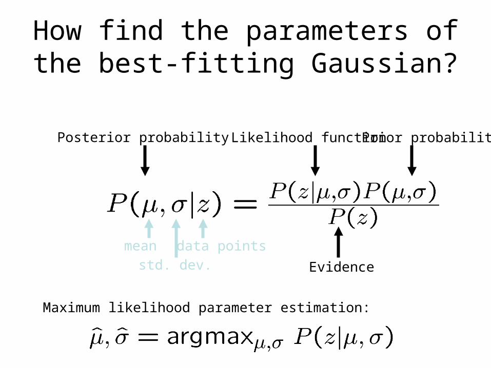
How find the parameters of the best-fitting Gaussian?

Posterior probability Likelihood function Prior probability

Evidence

Maximum likelihood parameter estimation:

mean

std. dev.

data points

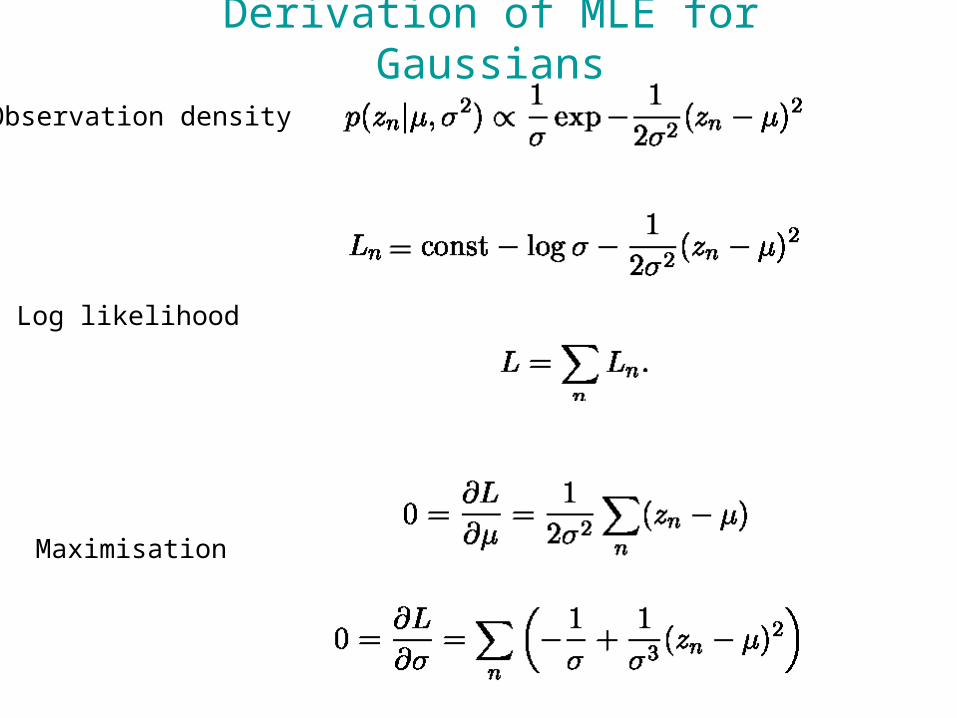
Derivation of MLE for Gaussians

Observation density

Log likelihood

Maximisation

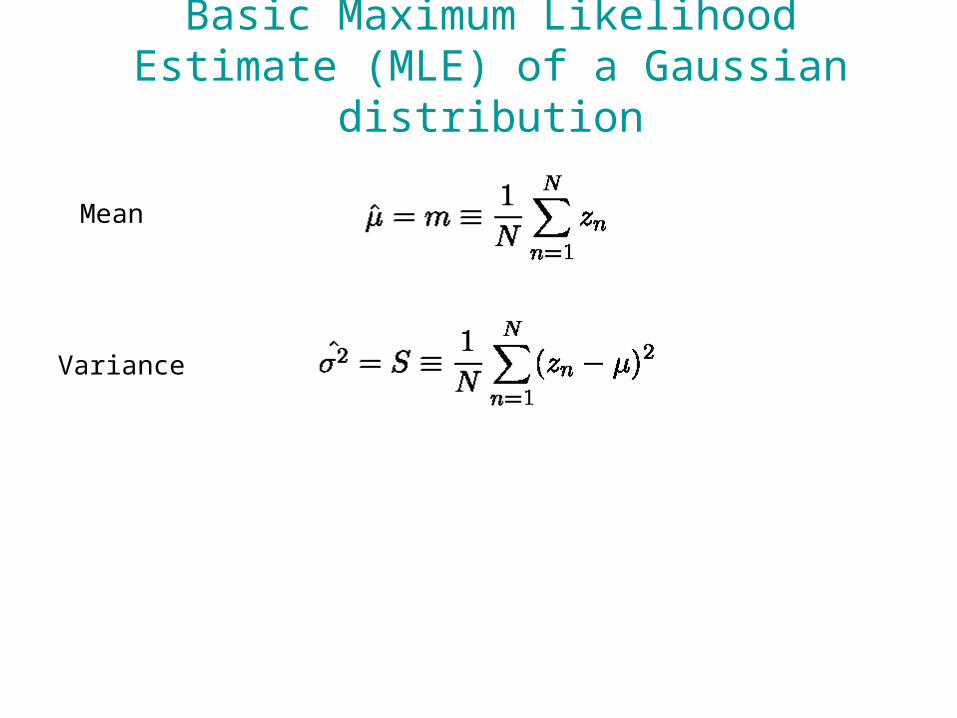
Basic Maximum Likelihood Estimate (MLE) of a Gaussian distribution

Mean

Variance

Covariance Matrix

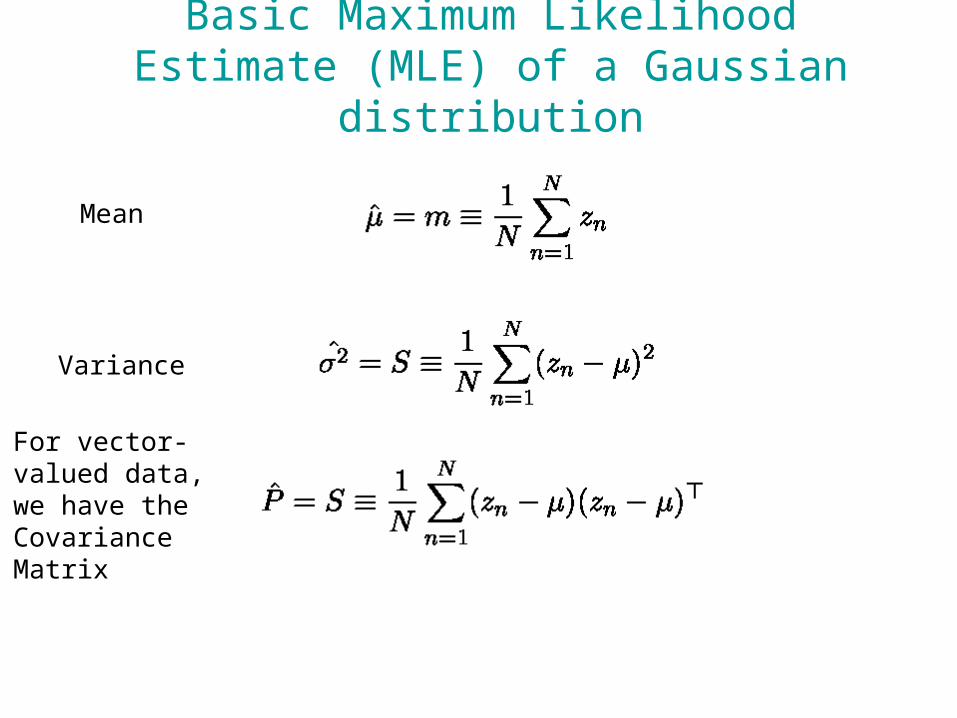
Basic Maximum Likelihood Estimate (MLE) of a Gaussian distribution

Mean

Variance

For vector-valued data,we have the Covariance Matrix

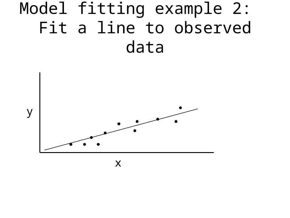
Model fitting example 2: Fit a line to observed data

x

y

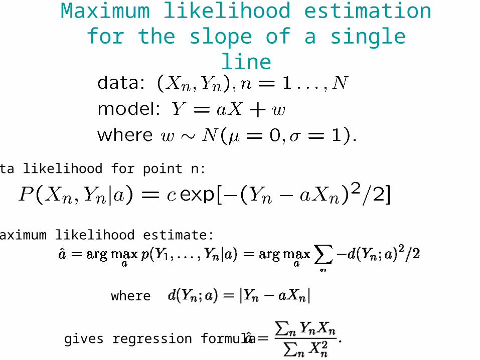
Maximum likelihood estimation for the slope of a single line

Maximum likelihood estimate:

where

gives regression formula

Data likelihood for point n:

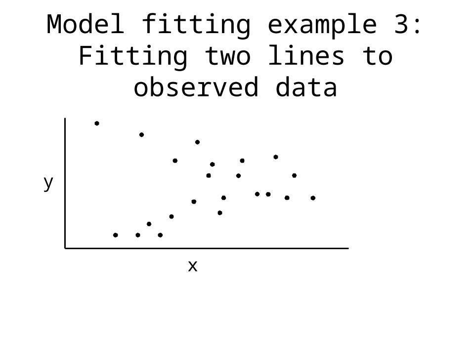
Model fitting example 3:Fitting two lines to observed data

x

y

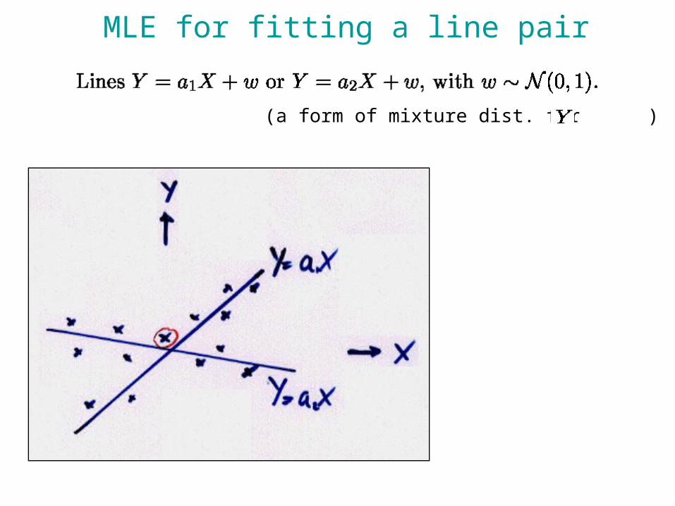
MLE for fitting a line pair

(a form of mixture dist. for )

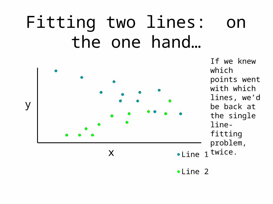
Fitting two lines: on the one hand…

x

y

If we knew which points went with which lines, we’d be back at the single line-fitting problem, twice.

Line 1

Line 2

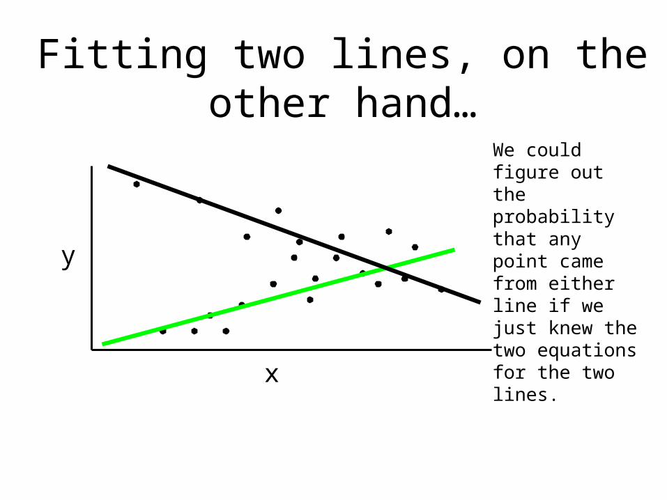
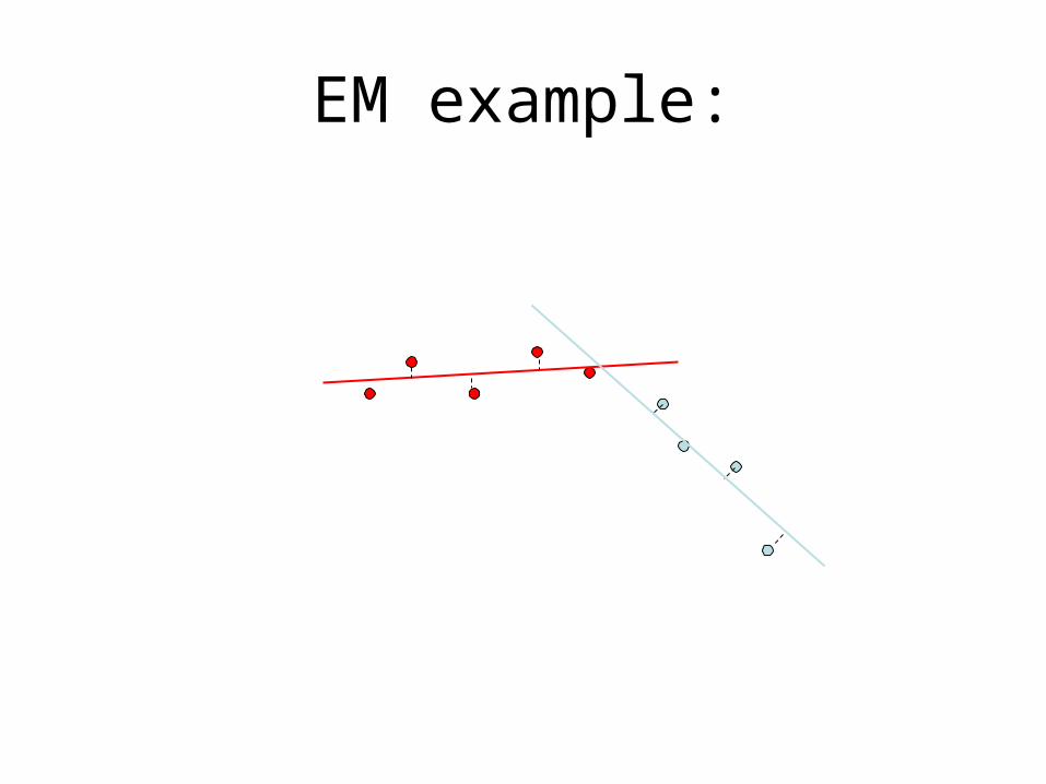
Fitting two lines, on the other hand…

x

y

We could figure out the probability that any point came from either line if we just knew the two equations for the two lines.

Expectation Maximization (EM): a solution to chicken-and-egg problems

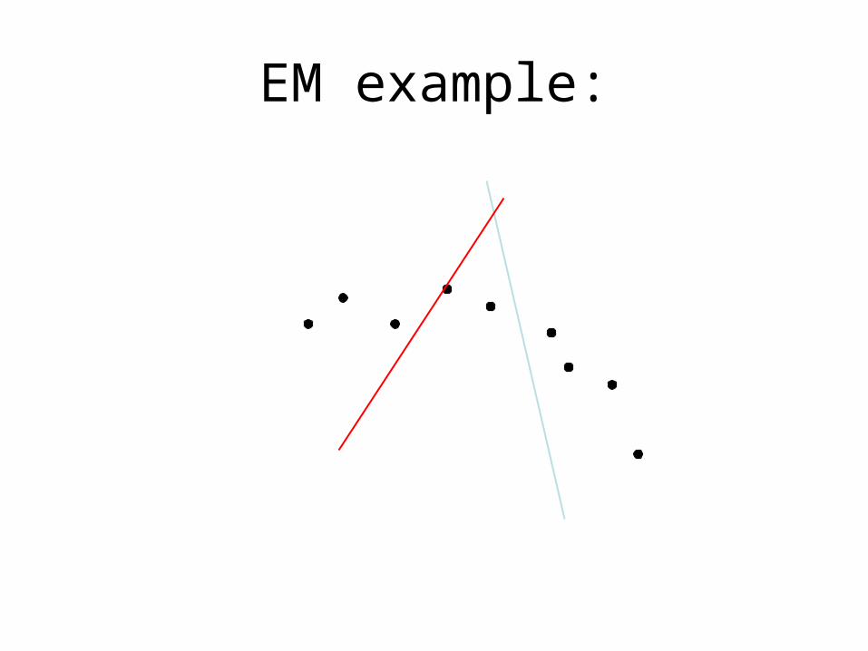
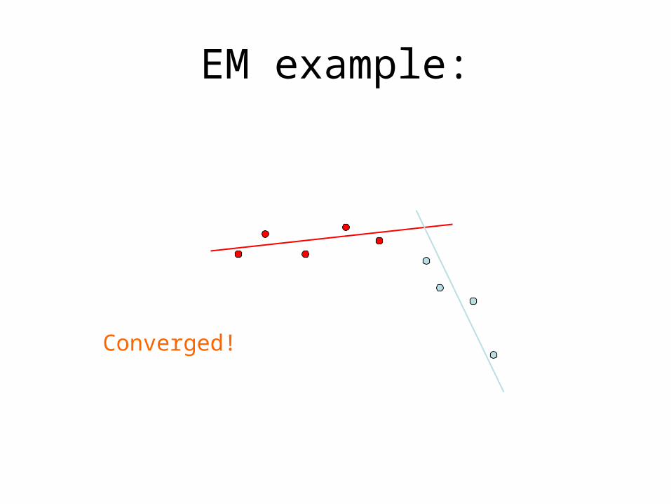
EM example:

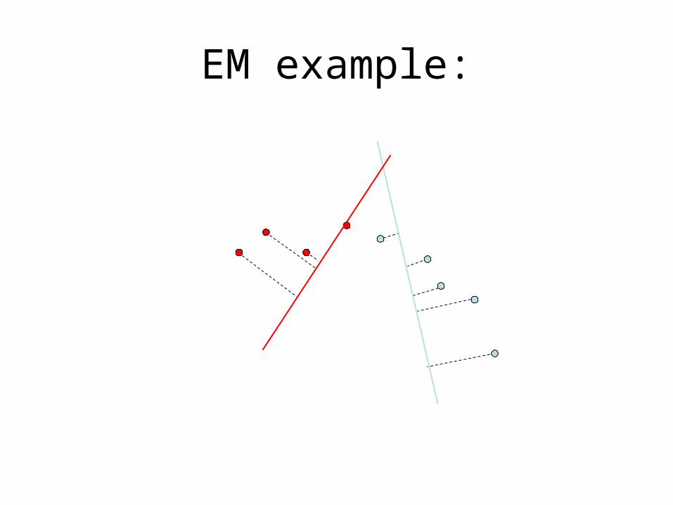
EM example:

EM example:

EM example:

EM example:

Converged!

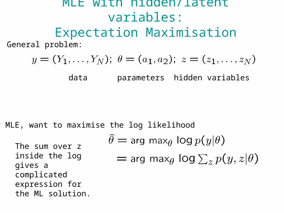
MLE with hidden/latent variables:Expectation Maximisation

General problem:

data parameters hidden variables

For MLE, want to maximise the log likelihood

The sum over z inside the log gives a complicated expression for the ML solution.

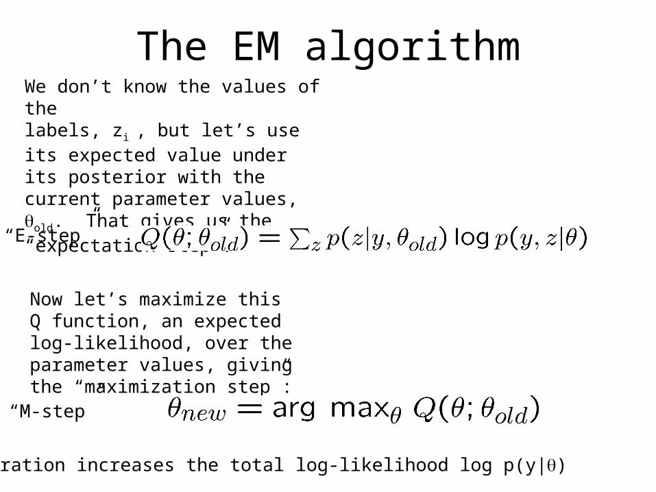
The EM algorithmWe don’t know the values of thelabels, zi , but let’s use its expected value under its posterior with the current parameter values, old. That gives us the “expectation step”:

“E-step”

“M-step”

Now let’s maximize this Q function, an expected log-likelihood, over the parameter values, giving the “maximization step”:

Each iteration increases the total log-likelihood log p(y|)

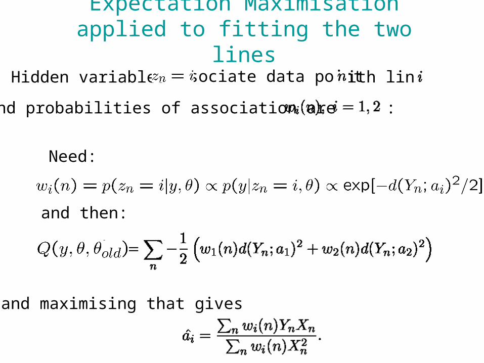
Expectation Maximisation applied to fitting the two lines

and maximising that gives

’ ’

Hidden variables associate data point with line

and probabilities of association are :

Need:

and then:

/2

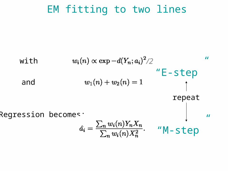
EM fitting to two lines

with

and

Regression becomes:

“E-step”

“M-step”

repeat

/2

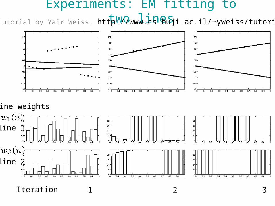
Experiments: EM fitting to two lines

Iteration 1 2 3

Line weights

line 1

line 2

(from a tutorial by Yair Weiss, http://www.cs.huji.ac.il/~yweiss/tutorials.html)

Applications of EM in computer vision

• Image segmentation

• Motion estimation combined with perceptual grouping

• Polygonal approximation of edges

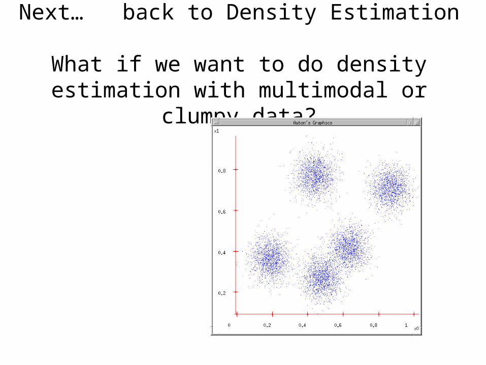
Next… back to Density Estimation

What if we want to do density estimation with multimodal or clumpy data?

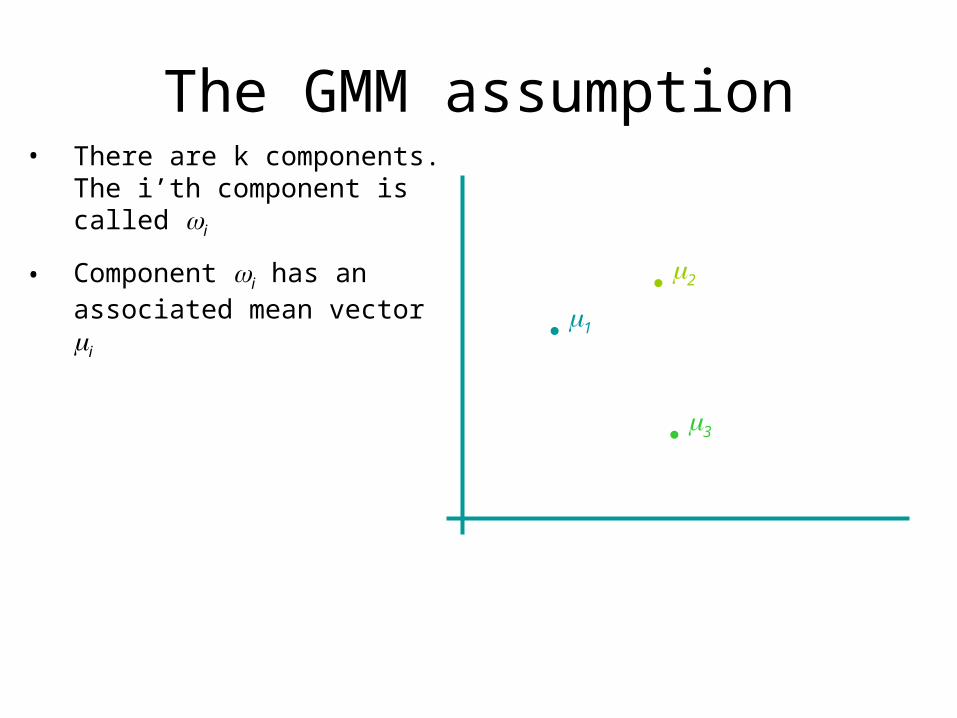
The GMM assumption• There are k components.

The i’th component is called i

• Component i has an associated mean vector i 1

2

3

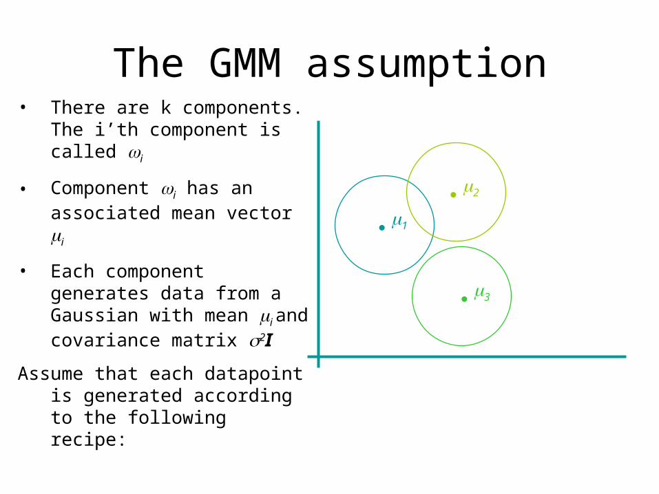
The GMM assumption• There are k components.

The i’th component is called i

• Component i has an associated mean vector i

• Each component generates data from a Gaussian with mean i and covariance matrix 2I

Assume that each datapoint is generated according to the following recipe:

1

2

3

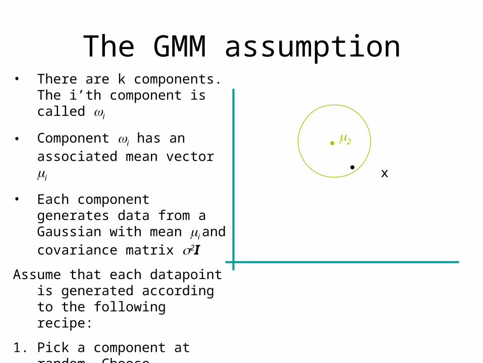
The GMM assumption• There are k components.

The i’th component is called i

• Component i has an associated mean vector i

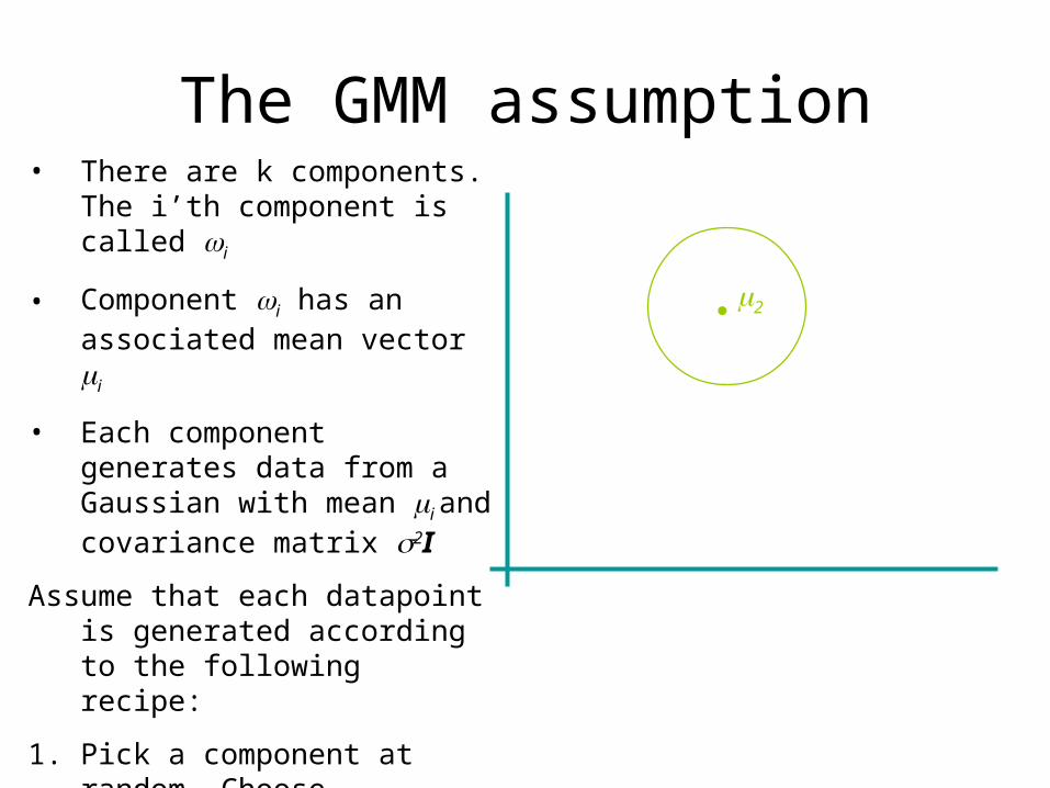
• Each component generates data from a Gaussian with mean i and covariance matrix 2I

Assume that each datapoint is generated according to the following recipe:

1. Pick a component at random. Choose component i with probability P(i).

2

The GMM assumption• There are k components.

The i’th component is called i

• Component i has an associated mean vector i

• Each component generates data from a Gaussian with mean i and covariance matrix 2I

Assume that each datapoint is generated according to the following recipe:

1. Pick a component at random. Choose component i with probability P(i).

2. Datapoint ~ N(i, 2I )

2

x

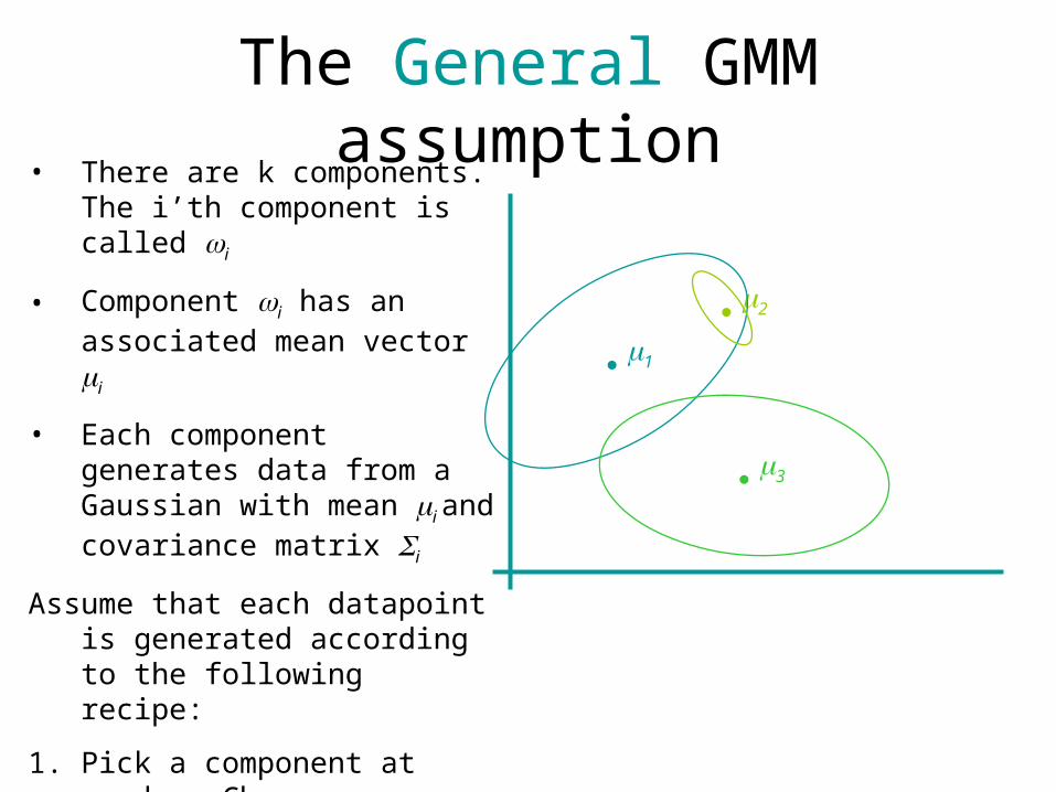
The General GMM assumption

1

2

3

• There are k components. The i’th component is called i

• Component i has an associated mean vector i

• Each component generates data from a Gaussian with mean i and covariance matrix i

Assume that each datapoint is generated according to the following recipe:

1. Pick a component at random. Choose component i with probability P(i).

2. Datapoint ~ N(i, i )

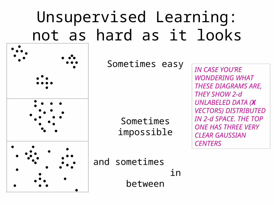
Unsupervised Learning:not as hard as it looks

Sometimes easy

Sometimes impossible

and sometimes in between

IN CASE YOU’RE WONDERING WHAT THESE DIAGRAMS ARE, THEY SHOW 2-d UNLABELED DATA (X VECTORS) DISTRIBUTED IN 2-d SPACE. THE TOP ONE HAS THREE VERY CLEAR GAUSSIAN CENTERS

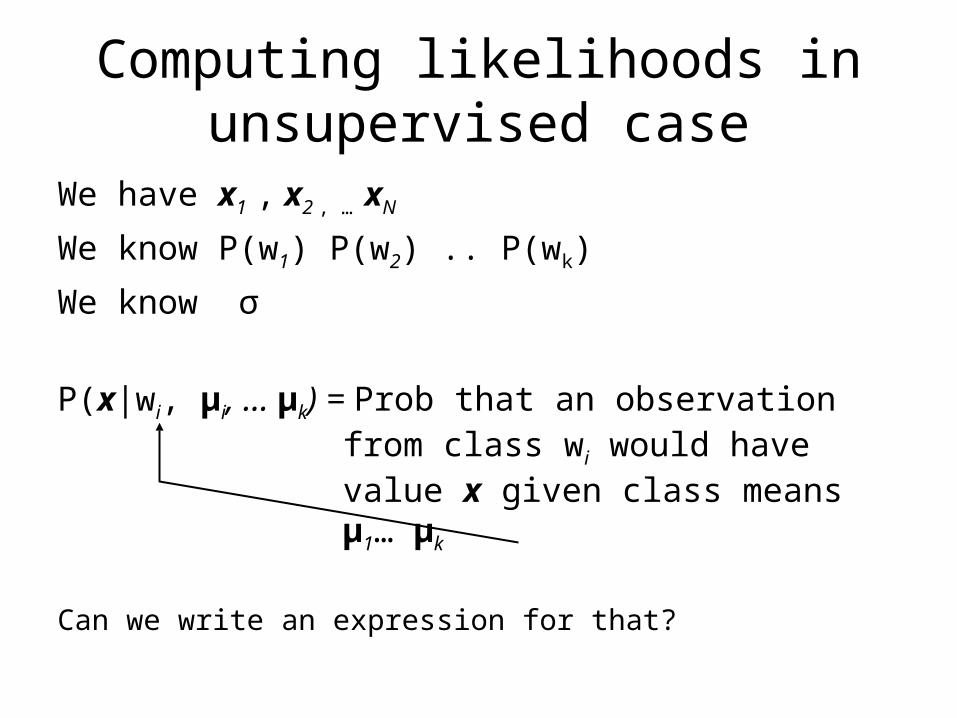
Computing likelihoods in unsupervised case

We have x1 , x2 , … xN

We know P(w1) P(w2) .. P(wk)

We know σ

P(x|wi, μi, … μk) = Prob that an observation from class wi would have value x given class means μ1… μk

Can we write an expression for that?

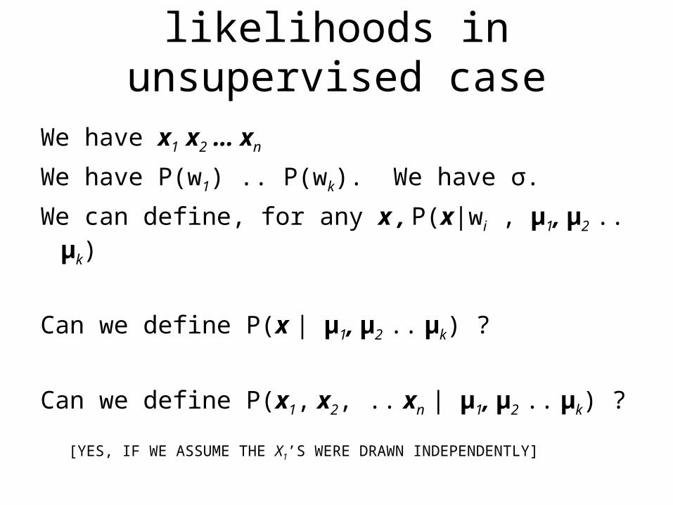
likelihoods in unsupervised case

We have x1 x2 … xn

We have P(w1) .. P(wk). We have σ.

We can define, for any x , P(x|wi , μ1, μ2 .. μk)

Can we define P(x | μ1, μ2 .. μk) ?

Can we define P(x1, x2, .. xn | μ1, μ2 .. μk) ?

[YES, IF WE ASSUME THE X1’S WERE DRAWN INDEPENDENTLY]

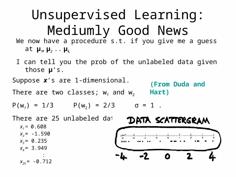
Unsupervised Learning:Mediumly Good News

We now have a procedure s.t. if you give me a guess at μ1, μ2 .. μk,

I can tell you the prob of the unlabeled data given those μ‘s.

Suppose x‘s are 1-dimensional.

There are two classes; w1 and w2

P(w1) = 1/3 P(w2) = 2/3 σ = 1 .

There are 25 unlabeled datapointsx1 = 0.608x2 = -1.590x3 = 0.235x4 = 3.949 :x25 = -0.712

(From Duda and Hart)

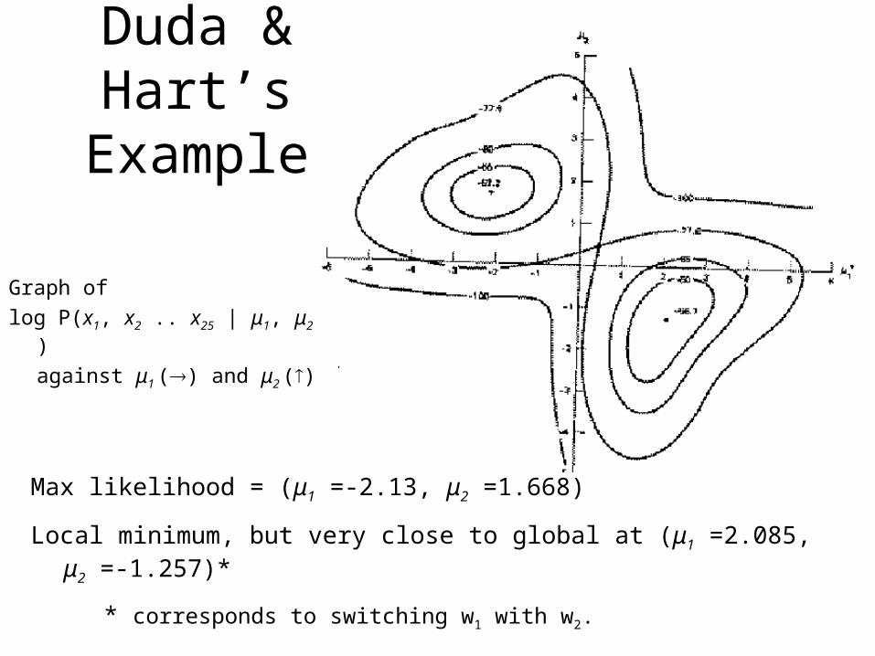
Graph of

log P(x1, x2 .. x25 | μ1, μ2 )

against μ1 () and μ2 ()

Max likelihood = (μ1 =-2.13, μ2 =1.668)

Local minimum, but very close to global at (μ1 =2.085, μ2 =-1.257)*

* corresponds to switching w1 with w2.

Duda & Hart’s

Example

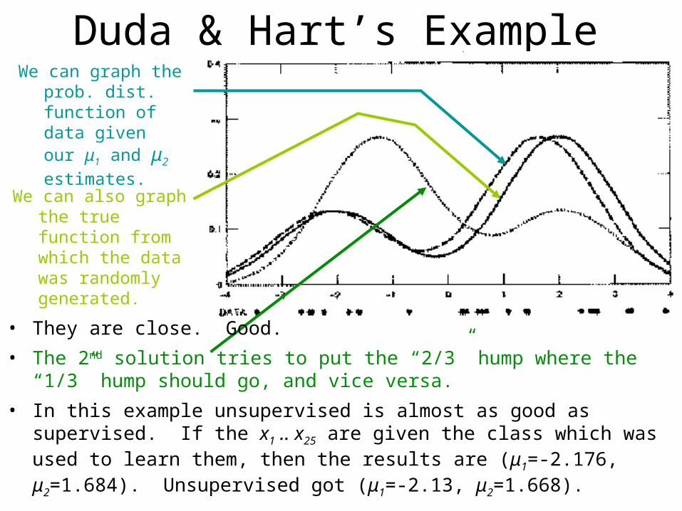
Duda & Hart’s ExampleWe can graph the

prob. dist. function of data given our μ1 and

μ2 estimates.

We can also graph the true function from which the data was randomly generated.

• They are close. Good.

• The 2nd solution tries to put the “2/3” hump where the “1/3” hump should go, and vice versa.

• In this example unsupervised is almost as good as supervised. If the x1 .. x25 are given the class which was used to learn them, then the results are (μ1=-2.176, μ2=1.684). Unsupervised got (μ1=-2.13, μ2=1.668).

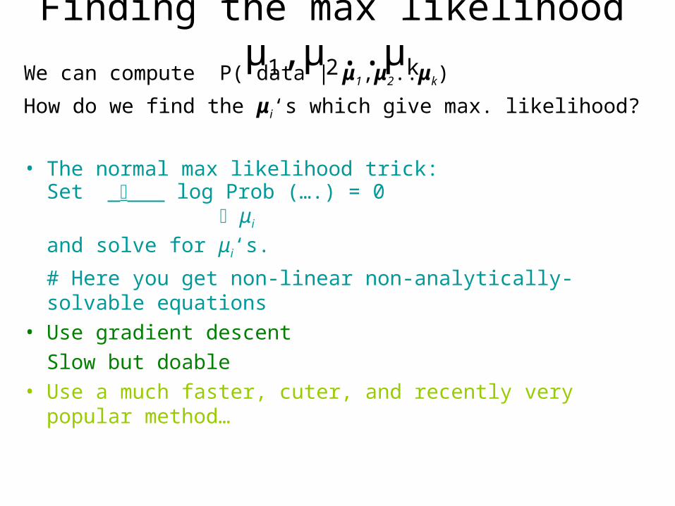
Finding the max likelihood μ1,μ2..μkWe can compute P( data | μ1,μ2..μk)

How do we find the μi‘s which give max. likelihood?

• The normal max likelihood trick:Set log Prob (….) = 0

μi

and solve for μi‘s.

# Here you get non-linear non-analytically-solvable equations

• Use gradient descent

Slow but doable• Use a much faster, cuter, and recently very popular

method…

Expectation Maximalization

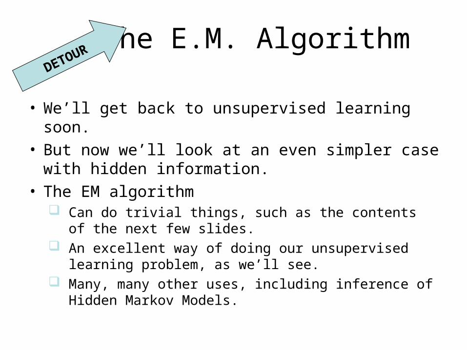
The E.M. Algorithm

• We’ll get back to unsupervised learning soon.• But now we’ll look at an even simpler case with

hidden information.• The EM algorithm

Can do trivial things, such as the contents of the next few slides.

An excellent way of doing our unsupervised learning problem, as we’ll see.

Many, many other uses, including inference of Hidden Markov Models.

DETOUR

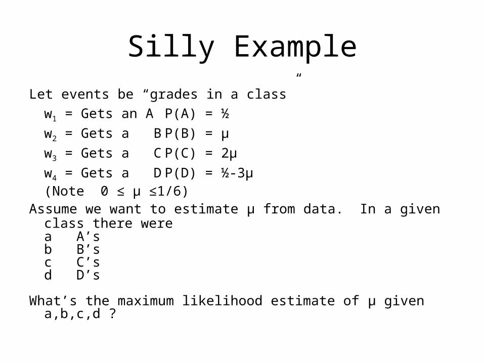
Silly Example

Let events be “grades in a class”

w1 = Gets an A P(A) = ½

w2 = Gets a B P(B) = μ

w3 = Gets a C P(C) = 2μ

w4 = Gets a D P(D) = ½-3μ(Note 0 ≤ μ ≤1/6)

Assume we want to estimate μ from data. In a given class there were

a A’sb B’sc C’sd D’s

What’s the maximum likelihood estimate of μ given a,b,c,d ?

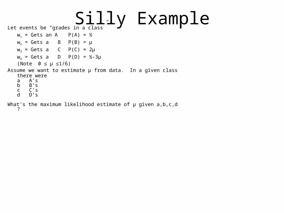
Silly ExampleLet events be “grades in a class”

w1 = Gets an A P(A) = ½

w2 = Gets a B P(B) = μ

w3 = Gets a C P(C) = 2μ

w4 = Gets a D P(D) = ½-3μ(Note 0 ≤ μ ≤1/6)

Assume we want to estimate μ from data. In a given class there werea A’sb B’sc C’sd D’s

What’s the maximum likelihood estimate of μ given a,b,c,d ?

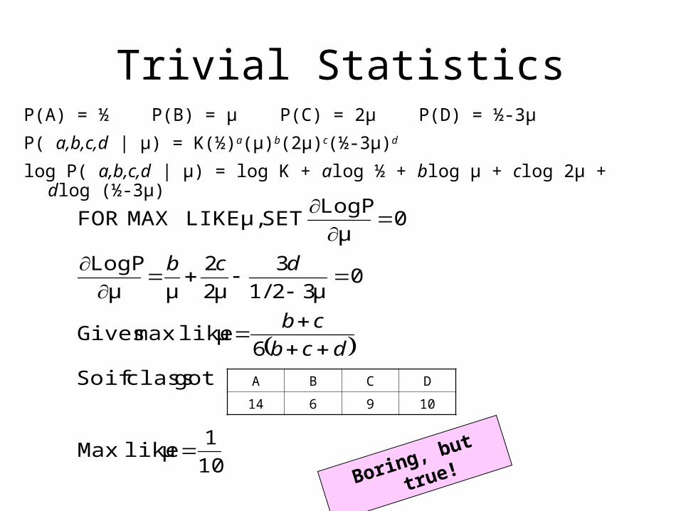
Trivial StatisticsP(A) = ½ P(B) = μ P(C) = 2μ P(D) = ½-3μ

P( a,b,c,d | μ) = K(½)a(μ)b(2μ)c(½-3μ)d

log P( a,b,c,d | μ) = log K + alog ½ + blog μ + clog 2μ + dlog (½-3μ)

10

1μ likeMax

got class if So

6 μ likemax Gives

0μ32/1

3

μ2

2

μμ

LogP

0μ

LogP SET μ, LIKE MAX FOR

dcb

cb

dcb

A B C D

14 6 9 10

Boring, but

true!

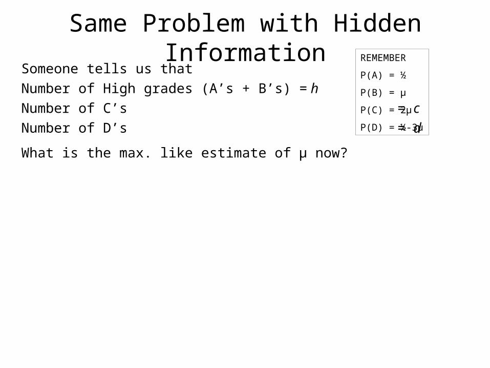
Same Problem with Hidden InformationSomeone tells us thatNumber of High grades (A’s + B’s) = hNumber of C’s = cNumber of D’s = d

What is the max. like estimate of μ now?

REMEMBER

P(A) = ½

P(B) = μ

P(C) = 2μ

P(D) = ½-3μ

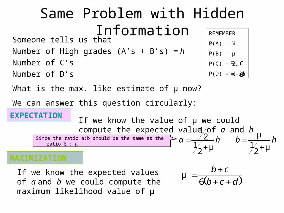
Same Problem with Hidden Information

hbhaμ2

1μ

μ2

12

1

dcb

cb

6

μ

Someone tells us thatNumber of High grades (A’s + B’s) = hNumber of C’s = cNumber of D’s = d

What is the max. like estimate of μ now?

We can answer this question circularly:

EXPECTATION

MAXIMIZATION

If we know the value of μ we could compute the expected value of a and b

If we know the expected values of a and b we could compute the maximum likelihood value of μ

REMEMBER

P(A) = ½

P(B) = μ

P(C) = 2μ

P(D) = ½-3μ

Since the ratio a:b should be the same as the ratio ½ :

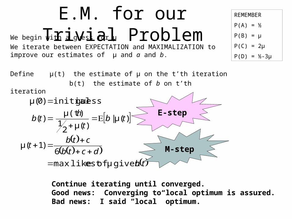
E.M. for our Trivial ProblemWe begin with a guess for μ

We iterate between EXPECTATION and MAXIMALIZATION to improve our estimates of μ and a and b.

Define μ(t) the estimate of μ on the t’th iteration

b(t) the estimate of b on t’th iteration

REMEMBER

P(A) = ½

P(B) = μ

P(C) = 2μ

P(D) = ½-3μ

tbdctb

ctbt

tbt

htb

given μ ofest likemax

6)1(μ

)(μ|)(μ2

1μ(t)

)(

guess initial )0(μ

E-step

M-step

Continue iterating until converged.Good news: Converging to local optimum is assured.Bad news: I said “local” optimum.

E.M. Convergence• Convergence proof based on fact that Prob(data | μ) must increase or

remain same between each iteration [NOT OBVIOUS]

• But it can never exceed 1 [OBVIOUS]

So it must therefore converge [OBVIOUS]

t μ(t) b(t)

0 0 0

1 0.0833 2.857

2 0.0937 3.158

3 0.0947 3.185

4 0.0948 3.187

5 0.0948 3.187

6 0.0948 3.187

In our example, suppose we had

h = 20c = 10d = 10

μ(0) = 0

Convergence is generally linear: error decreases by a constant factor each time step.

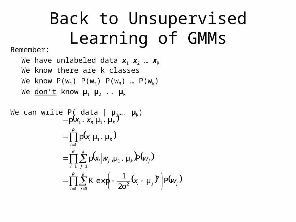
Back to Unsupervised Learning of GMMs

Remember:

We have unlabeled data x1 x2 … xR

We know there are k classes

We know P(w1) P(w2) P(w3) … P(wk)

We don’t know μ1 μ2 .. μk

We can write P( data | μ1…. μk)

R

i

k

jjji

R

i

k

jjkji

R

iki

kR

wx

wwx

x

xx

1 1

2

2

1 11

11

11

Pμσ2

1expK

Pμ...μ,p

μ...μp

μ...μ...p

E.M. for GMMs

R

ikij

i

R

ikij

j

ki

xwP

xxwP

11

11

1

μ...μ,

μ...μ, μ

j,each for ,likelihoodMax For " :into this turnsalgebracrazy n' wild'Some

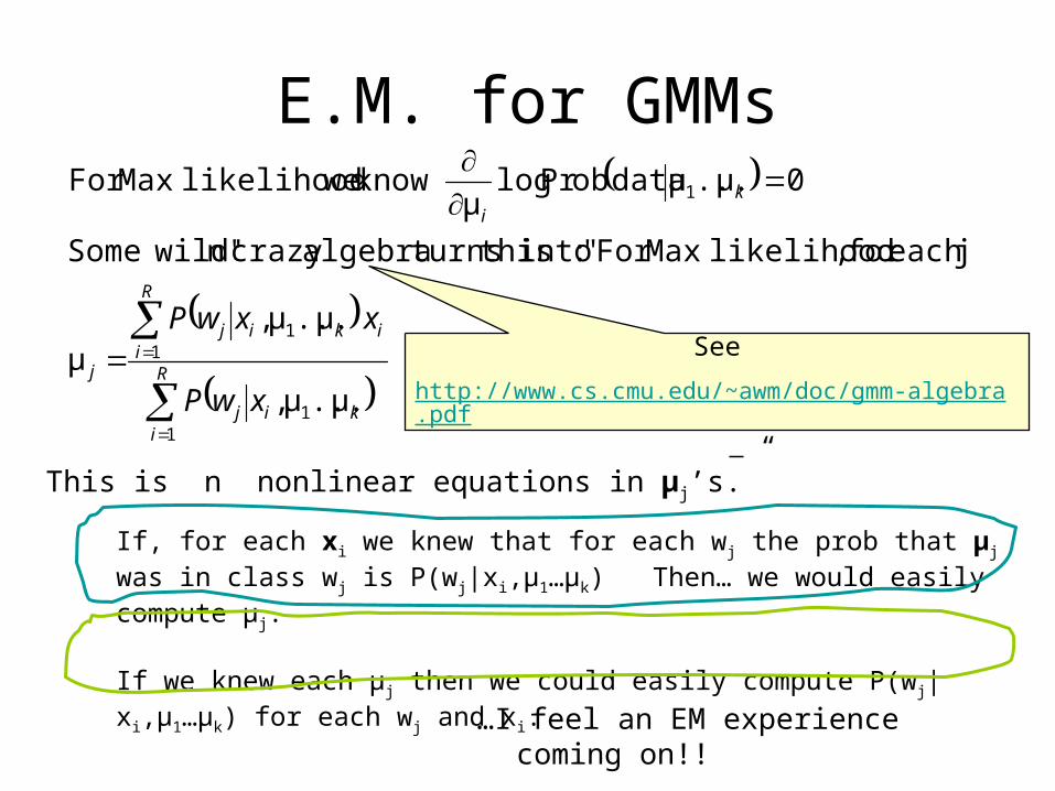
0μ...μdataobPrlogμ

know welikelihoodMax For

This is n nonlinear equations in μj’s.”

…I feel an EM experience coming on!!

If, for each xi we knew that for each wj the prob that μj was in class wj is P(wj|xi,μ1…μk) Then… we would easily compute μj.

If we knew each μj then we could easily compute P(wj|xi,μ1…μk) for each wj and xi.

See

http://www.cs.cmu.edu/~awm/doc/gmm-algebra.pdf

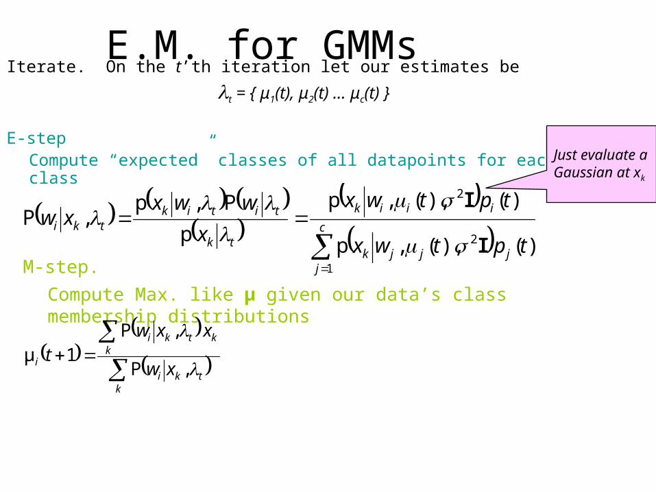
E.M. for GMMsIterate. On the t’th iteration let our estimates be

t = { μ1(t), μ2(t) … μc(t) }

E-stepCompute “expected” classes of all datapoints for each class

c

jjjjk

iiik

tk

titiktki

tptwx

tptwx

x

wwxxw

1

2

2

)(),(,p

)(),(,p

p

P,p,P

I

I

M-step.

Compute Max. like μ given our data’s class membership distributions

ktki

kk

tki

i xw

xxwt

,P

,P1μ

Just evaluate a Gaussian at xk

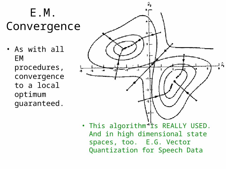
E.M. Convergence

• This algorithm is REALLY USED. And in high dimensional state spaces, too. E.G. Vector Quantization for Speech Data

• As with all EM procedures, convergence to a local optimum guaranteed.

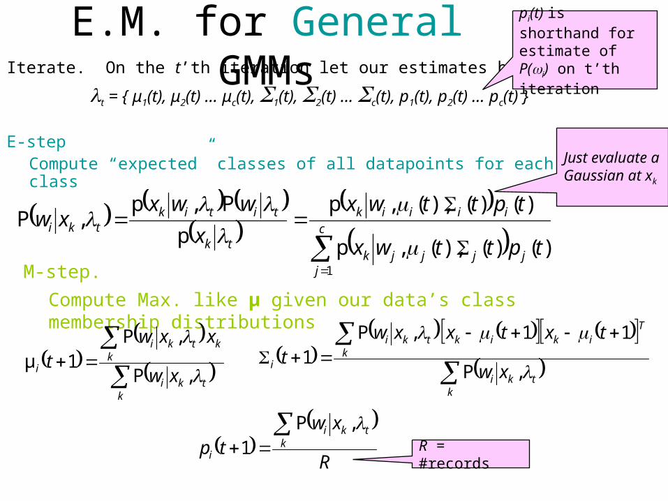
E.M. for General GMMsIterate. On the t’th iteration let our estimates be

t = { μ1(t), μ2(t) … μc(t), 1(t), 2(t) … c(t), p1(t), p2(t) … pc(t) }

E-stepCompute “expected” classes of all datapoints for each class

c

jjjjjk

iiiik

tk

titiktki

tpttwx

tpttwx

x

wwxxw

1

)()(),(,p

)()(),(,p

p

P,p,P

M-step.

Compute Max. like μ given our data’s class membership distributions

pi(t) is shorthand for estimate of P(i) on t’th iteration

ktki

kk

tki

i xw

xxwt

,P

,P1μ

ktki

Tikik

ktki

i xw

txtxxwt

,P

11 ,P1

R

xwtp k

tki

i

,P1 R = #records

Just evaluate a Gaussian at xk

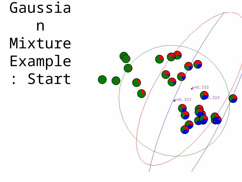
Gaussian Mixture

Example: Start

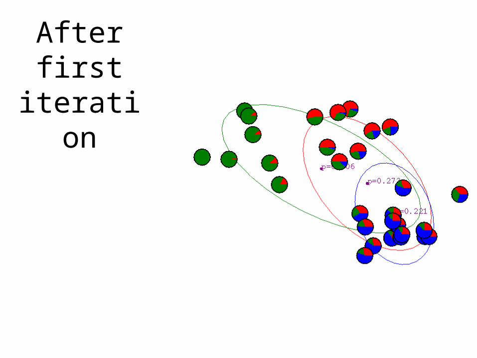
After first iteration

After 2nd iteration

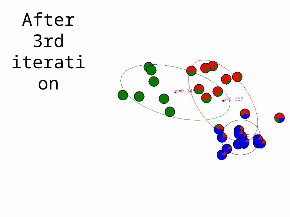
After 3rd iteration

After 4th iteration

After 5th iteration

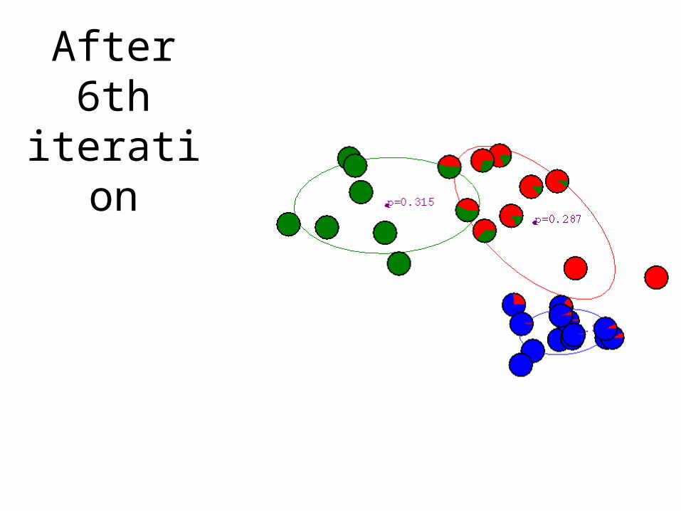
After 6th iteration

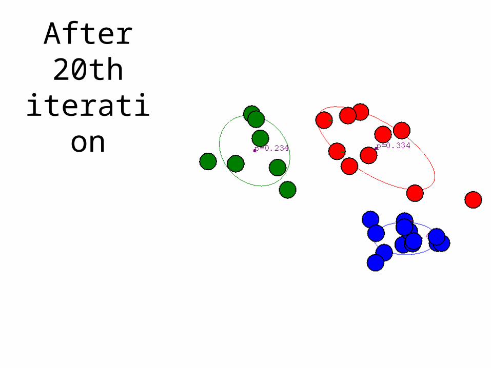
After 20th iteration

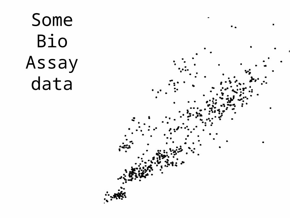
Some Bio Assay data

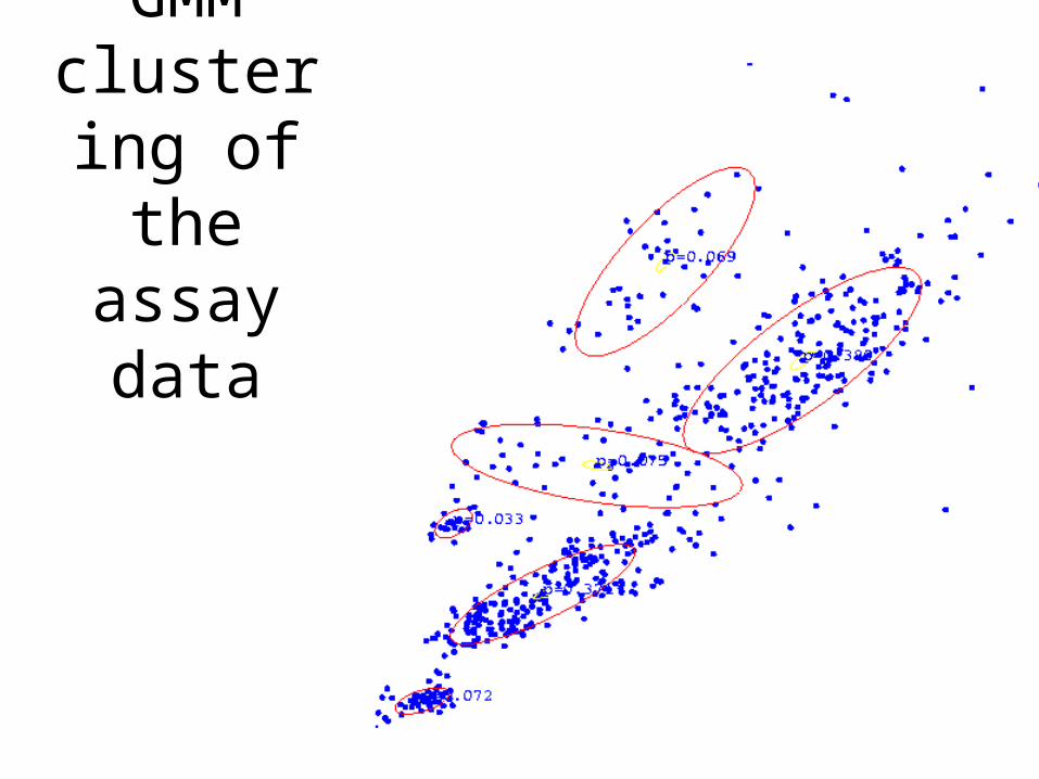
GMM clustering

of the assay data

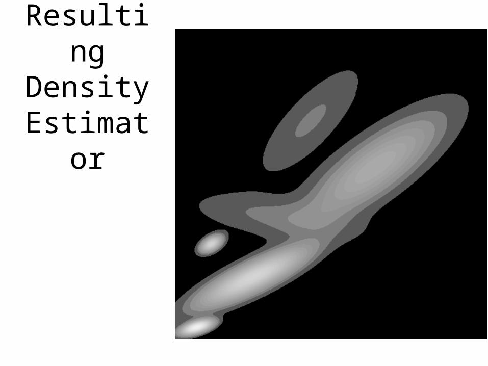
Resulting Density

Estimator

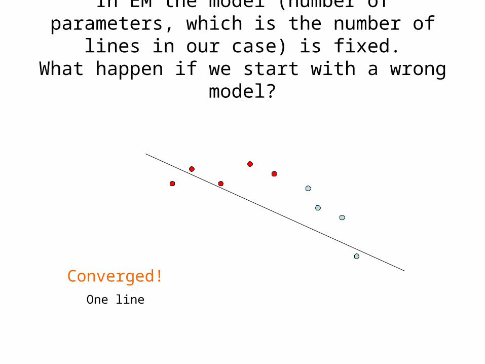
In EM the model (number of parameters, which is the number of lines in our case) is fixed.

What happen if we start with a wrong model?

One line

Converged!

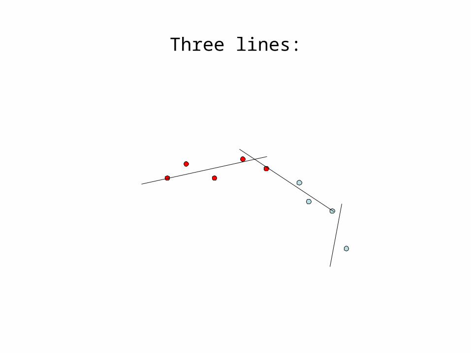
Three lines:

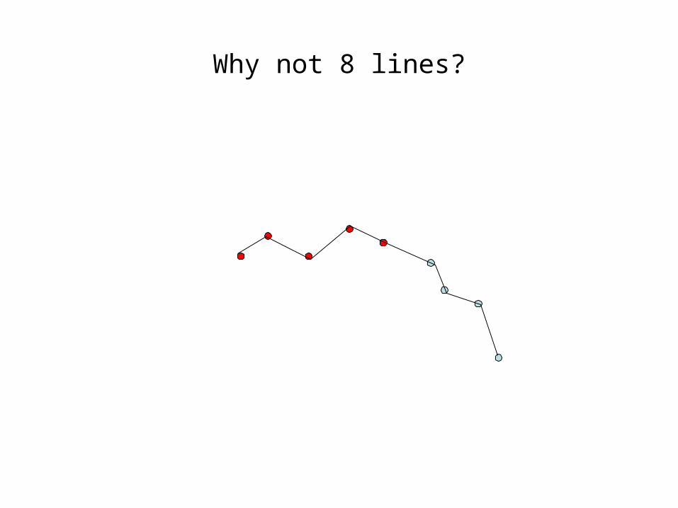
Why not 8 lines?

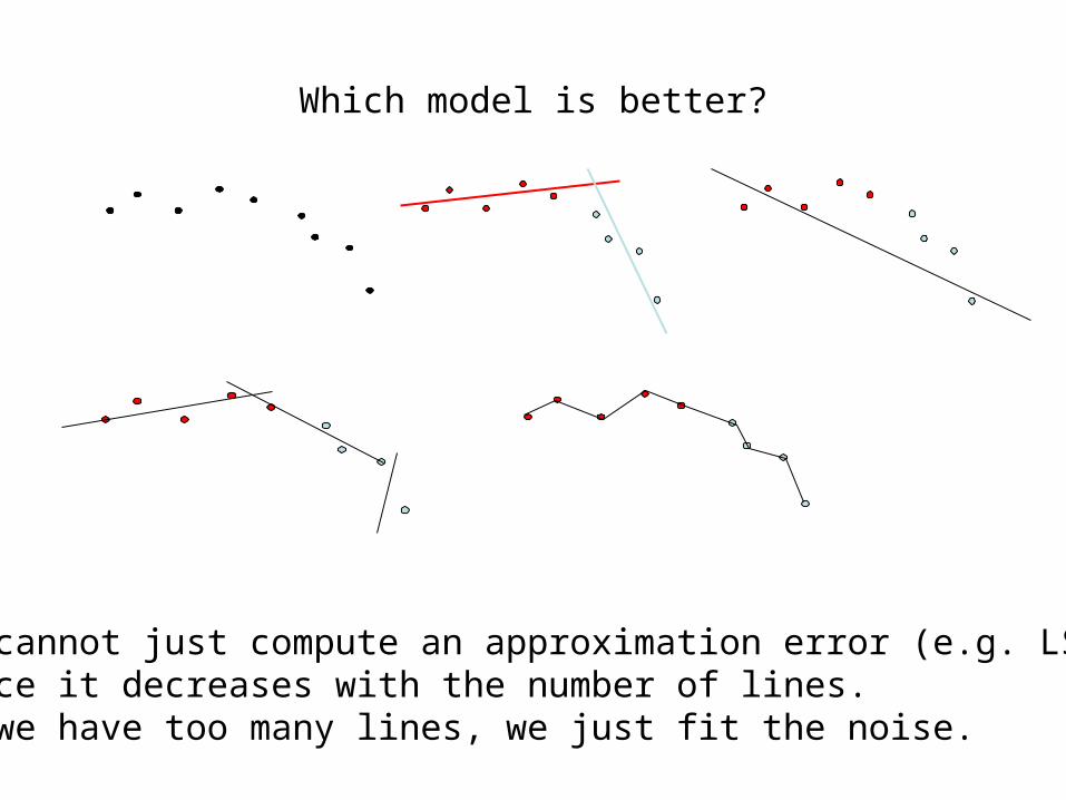
Which model is better?

We cannot just compute an approximation error (e.g. LSE),since it decreases with the number of lines.If we have too many lines, we just fit the noise.

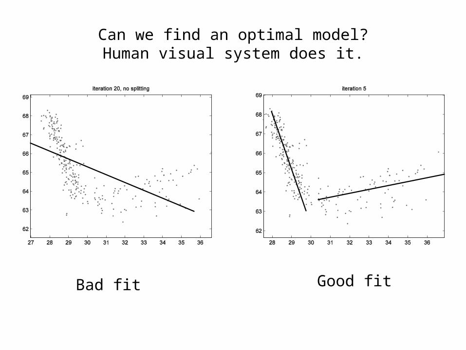
Can we find an optimal model?Human visual system does it.

Bad fit Good fit

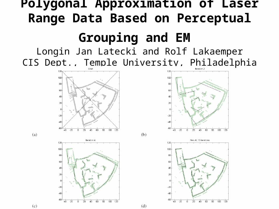
Polygonal Approximation of Laser Range Data

Based on Perceptual Grouping and EM Longin Jan Latecki and Rolf Lakaemper

CIS Dept., Temple University, Philadelphia

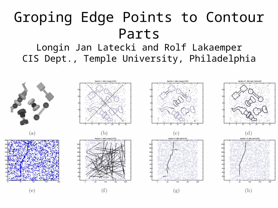
Groping Edge Points to Contour PartsLongin Jan Latecki and Rolf Lakaemper

CIS Dept., Temple University, Philadelphia