introduction to saga gis - iget - homedst-iget.in/tutorials/iget_rs_001/iget_rs_001 introduction to...

Introduction to SAGA GIS

Tutorial ID: IGET_RS_001

This tutorial has been developed by BVIEER as part of the IGET web portal intended to provide easy access to geospatial education. This tutorial is released under the Creative Commons license. Your support will help our team to improve the content and to continue to offer high quality geospatial educational resources. For suggestions and feedback please visit www.dst-iget.in.

IGET_RS_001 Introduction to SAGA

2

Introduction to SAGA GIS

Objective: To get familiar with SAGA GIS interface and view and explore raster data in it. Software: SAGA GIS (2.1.0) Level: Beginner Time required: 3 Hours Prerequisites and Geospatial Skills

1. SAGA should be installed on the computer Reading

--

Tutorial Data: The image required for this exercise may be downloaded from IGET_RS_001

SAGA 2.0.1 can be downloaded from http://sourceforge.net/projects/saga-

gis/files/latest/download?source=directory. After downloading the file, unzip it to a convenient

location.


3

Introduction

SAGA (System for Automated Geoscientific Analyses) is an open-source digital image

processing GIS program capable of processing images in different formats. It uses the well

established GDAL/OGR library to import and export images to and from its native format,

SAGA Grid (*.sgrd).

In this tutorial, we will use imagery from the LISS 3 sensor. This image is a composite of 4

bands i.e. Band 2 (Green), Band 3 (Red), Band 4 (Near IR) and Band 5(Shortwave IR). The

image covers the city of Pune along with some parts of the Western Ghats of Maharashtra. In

this tutorial we will learn how to handle, view and save raster data.

1. SAGA is available as a stand-alone program which means it does not have an

installation procedure. To start SAGA, navigate to the SAGA folder, look for the

'saga_gui.exe' icon and double-click on it.

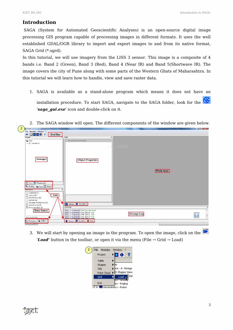
2. The SAGA window will open. The different components of the window are given below.

3. We will start by opening an image in the program. To open the image, click on the

'Load' button in the toolbar, or open it via the menu (File → Grid → Load)

2

3


4

4. This will open a window from where we must navigate to our image folder. The images

may not be immediately visible. At the bottom right of the window beside File name,

there will be a drop down menu. Change the selection to 'All Files'. The 4 layers will

now be visible. Select all of them and click 'Open'. This imports the images into

temporary *.sgrd images.

5. To see the list of these images, click on the Data tab in the Workspace module. This

tab displays all the data that has been loaded into SAGA. In SAGA, raster data is

stored in a grid system. Each grid system contains images having the same pixel size,

4

6

4


5

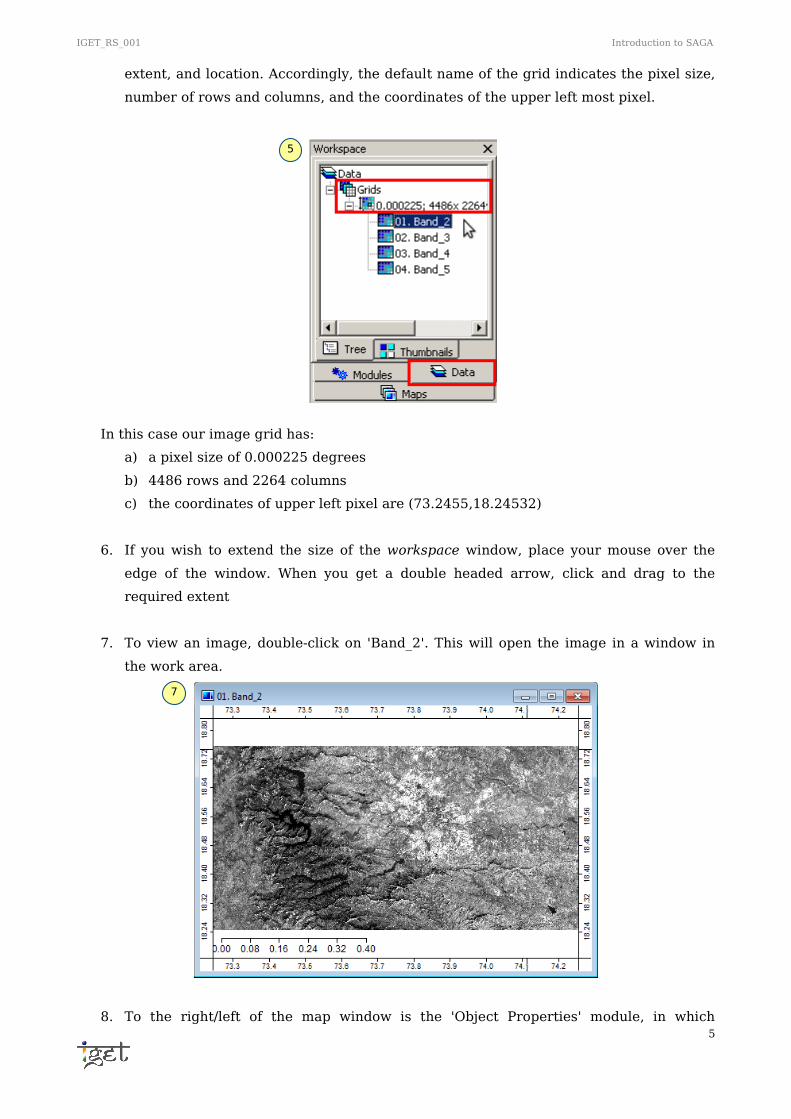
extent, and location. Accordingly, the default name of the grid indicates the pixel size,

number of rows and columns, and the coordinates of the upper left most pixel.

In this case our image grid has:

a) a pixel size of 0.000225 degrees

b) 4486 rows and 2264 columns

c) the coordinates of upper left pixel are (73.2455,18.24532)

6. If you wish to extend the size of the workspace window, place your mouse over the

edge of the window. When you get a double headed arrow, click and drag to the

required extent

7. To view an image, double-click on 'Band_2'. This will open the image in a window in

the work area.

8. To the right/left of the map window is the 'Object Properties' module, in which

5

7


6

information about the image is displayed. The different tabs of this module are

described below:

a) Setings: Options related to the display of the data are found here.

b) Decription: Description of the projection, geometry, extent, values and size of the

data selected.

c) Legend: Displays the legend style of the data

d) History: Maintains a log of all the operations and changes carried out on this

layer.

e) Attributes: This lists out the attributes of the selected data layer.

9. You might notice that on opening the image, another toolbar appears. This is 'Map'

toolbar, and it contains some basic tools used in layer navigation and display.

10. Click on the 'Zoom' button and then click and drag on the map to zoom in to a

particular area (Alternately, we may use the mouse scroll wheel to zoom in and out).

Zoom to the pixel level where every pixel can be easily distinguished from its

neighbour.

11. In the Object Properties section, under ‘Settings’ tab there will be a field titled 'Show

Cell Values' . Click on the check box next to it, and click on the

'Apply' button below.

12. You will see that the pixels in the image are labeled with their Digital Number values,

the higher values being lighter and the lower values being darker.

12


7

13. To move around the map click on the 'Pan' button and then click and drag the

map.

14. The cell values can also be viewed as a table/spreadsheet. Click on the

Attributes tab and then select the 'Action' cursor form the Toolbar.

Click and drag on the map. A rectangle will be drawn out which will encompass a few

pixels.

15. The current colour ramp of the layers is black → white. We may assign a different

colour ramp by clicking on the 'Settings' tab. Under the heading

'Graduated Colour' is the entry 'Colors'. Next to this is the current colour ramp

which looks like this → . Select it and then click on the button which

appears on its right.

16. A Colours window appears, having 3 primary colour ramps which we can use to

create our ramp. However, for now we will use a preset colour ramp. Click on

'Presets' and select 'Rainbow' from the Preset Selection List and click ‘OK’. Click

'Okay'. The settings of the layer will now look like this:

16

14


8

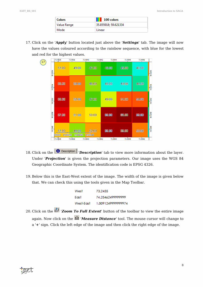
17. Click on the 'Apply' button located just above the 'Settings' tab. The image will now

have the values coloured according to the rainbow sequence, with blue for the lowest

and red for the highest values.

18. Click on the 'Description' tab to view more information about the layer.

Under 'Projection' is given the projection parameters. Our image uses the WGS 84

Geographic Coordinate System. The identification code is EPSG 4326.

19. Below this is the East-West extent of the image. The width of the image is given below

that. We can check this using the tools given in the Map Toolbar.

20. Click on the 'Zoom To Full Extent' button of the toolbar to view the entire image

again. Now click on the 'Measure Distance' tool. The mouse cursor will change to

a '+' sign. Click the left edge of the image and then click the right edge of the image.

17


9

21. A line will be drawn out between the two points. At the bottom of the screen will be

the measured distance between the two points. Besides this is the current position of

the cursor . In this case it should be approximately

equal to 1, ie. The image width is around 1 degree.

Task 1: Now do the same for the North-South extent of the image. What value do you get?

22. The current view of the data list is in the tree structure. SAGA lets you preview data as

thumbnails by clicking on the 'Thumbnails' tab next to the 'Tree' tab. This way we

can browse the images visually.

22

20

21


10

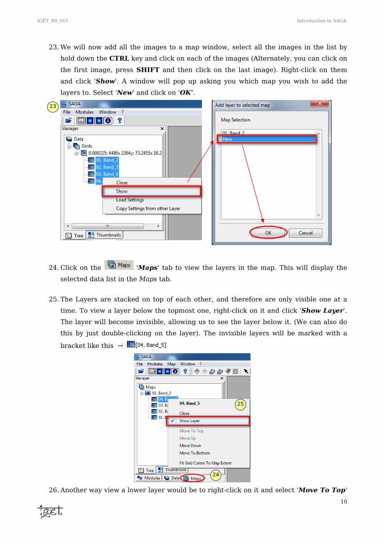
23. We will now add all the images to a map window, select all the images in the list by

hold down the CTRL key and click on each of the images (Alternately, you can click on

the first image, press SHIFT and then click on the last image). Right-click on them

and click 'Show'. A window will pop up asking you which map you wish to add the

layers to. Select 'New' and click on 'OK'.

24. Click on the 'Maps' tab to view the layers in the map. This will display the

selected data list in the Maps tab.

25. The Layers are stacked on top of each other, and therefore are only visible one at a

time. To view a layer below the topmost one, right-click on it and click 'Show Layer'.

The layer will become invisible, allowing us to see the layer below it. (We can also do

this by just double-clicking on the layer). The invisible layers will be marked with a

bracket like this →

26. Another way view a lower layer would be to right-click on it and select 'Move To Top'

23

24

25


11

from the dropdown menu.

27. The layer transparency can also be changed by clicking on the ‘Settings’ tab on the

right and then clicking on the space next to ‘Transparency’. Type in the required

transparency (Set it to 100 to make the layer invisible) then press ‘Tab’ in Keyboard.

Click on ‘Apply’.

28. You may find that apart from the basic shapes, interpreting the image and the type of

land cover is not possible by viewing it one band at a time. For this, we will need to

view the image as a false colour composite.

29. SAGA cannot handle multi-band imagery. The layers have to be viewed individually.

Therefore for every band combination, a false colour composite must be created as a

separate image, or must overwrite a previous image.

30. Load the RGB Composite module via the Menu (Modules → Grid → Visualisation → RGB

Composite)

31. The 'RGB Composite' window will open in which will assign a band to each of the 3

colours. Click on the dropdown menu next to 'Grid System' and select the grid system

to be used. Below this will be the entries for the colours. Using the dropdown menus

select the appropriate bands for each colour. We will use the bands 4, 3 and 2 for Red,

Green, and Blue respectively. Click 'Okay'.

31


12

32. The composite is loaded into the same grid system as the rest of the layers. Click on

the Data tab and double-click on the layer titled 'Composite'. Add it into a new map.

The composite will like below.

Note: If the Composite appears in grey ramp, go to the ‘Settings’ tab, under ‘Colours’ section

select ‘Type’ as ‘RGB’.

33. The composite makes it easier for us to interpret the image. For example, the red

patches indicate the presence of vegetation, while the large black patched are water

bodies.

34. To change the band combinations run the 'RGB Composite' module again. From the

Menu select Module and look at the last entry. It will display the most recently used

processing module.

32

34

33


13

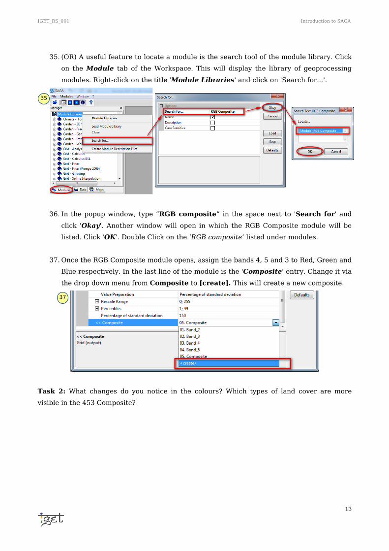
35. (OR) A useful feature to locate a module is the search tool of the module library. Click

on the Module tab of the Workspace. This will display the library of geoprocessing

modules. Right-click on the title 'Module Libraries' and click on 'Search for...'.

36. In the popup window, type “RGB composite” in the space next to 'Search for' and

click 'Okay'. Another window will open in which the RGB Composite module will be

listed. Click 'OK'. Double Click on the ‘RGB composite’ listed under modules.

37. Once the RGB Composite module opens, assign the bands 4, 5 and 3 to Red, Green and

Blue respectively. In the last line of the module is the 'Composite' entry. Change it via

the drop down menu from Composite to [create]. This will create a new composite.

Task 2: What changes do you notice in the colours? Which types of land cover are more

visible in the 453 Composite?

35

37


14

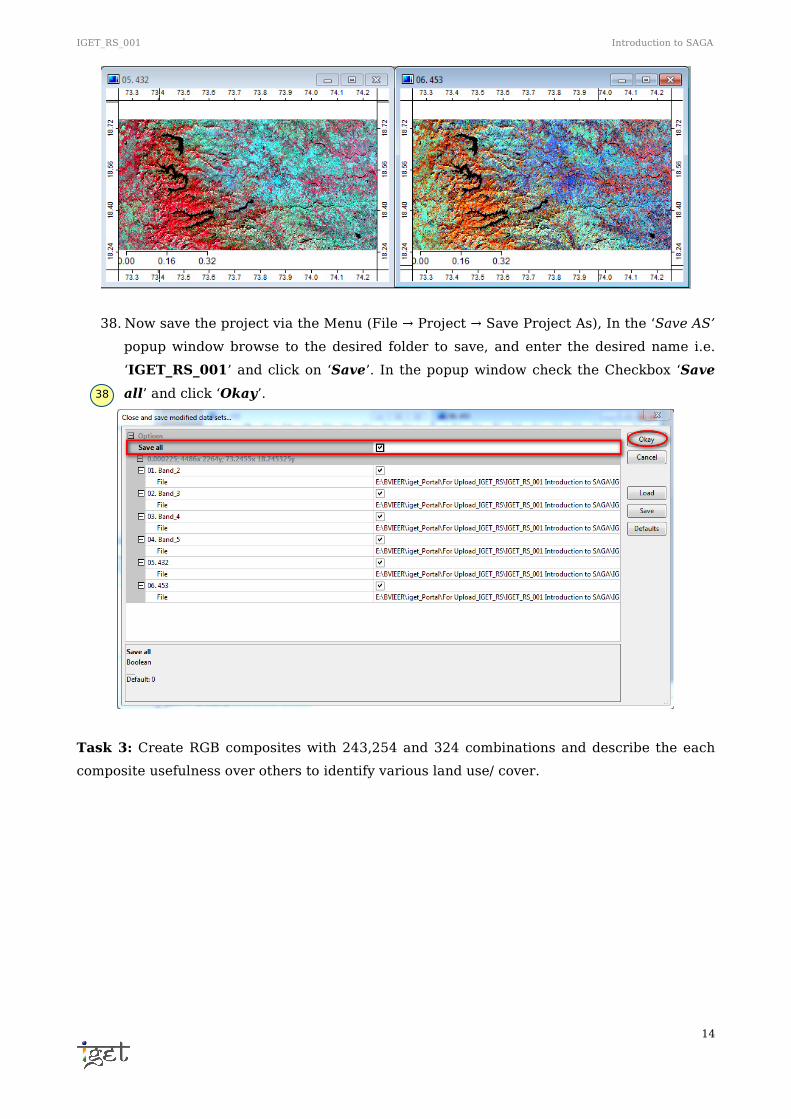
38. Now save the project via the Menu (File → Project → Save Project As), In the ‘Save AS’

popup window browse to the desired folder to save, and enter the desired name i.e.

‘IGET_RS_001’ and click on ‘Save’. In the popup window check the Checkbox ‘Save

all’ and click ‘Okay’.

Task 3: Create RGB composites with 243,254 and 324 combinations and describe the each

composite usefulness over others to identify various land use/ cover.

38

introduction to saga gis - iget - homedst-iget.in/tutorials/iget_rs_001/iget_rs_001 introduction to...

Documents