inventory and financial strategies with capital
TRANSCRIPT

Inventory and Financial Strategies with CapitalConstraints and Limited Joint Liability
Bin CaoSchool of Business Administration, South China University of Technology, Guangzhou, China,
Xin ChenDepartment of Industrial Enterprise and Systems Engineering, University of Illinois at Urbana-Champaign,
Urbana, Illinois, [email protected]
T.C.E. ChengDepartment of Logistics and Maritime Studies, The Hong Kong Polytechnic University, Hong Kong, China,
Yuanguang Zhong, Yong-Wu ZhouSchool of Business Administration, South China University of Technology, Guangzhou, China,
[email protected], zyw [email protected]
We study the financial and operational decisions of two capital-constrained firms via a limited joint liability
(LJL) financing scheme offered by a bank. To explicitly assess the value of the LJL financing scheme, we
assume that the firms either use their own initial capital (also called the self-financing scheme) or the LJL
financing scheme to support their operations. We provide a framework on how the firms react to the LJL
financing scheme and how the bank sets the loan terms (e.g., the credit line) based on the the capital in
the pool committed by the firms. We derive a two-stage model in which the firms separately determine
their individual ordering decisions according to the prior joint liability agreement between the firms and
the bank. Applying a non-cooperative game to analyze the decision-making problems of the two firms, we
establish the existence of equilibrium decisions for the two firms. We characterize the mild conditions under
which the LJL financing scheme is simultaneously preferred by the two firms. We show that the two firms’
strategies are complementary and the firms’ equilibrium order quantities are always positively influenced
by the risk-sharing terms. We find that a greater bank loan leverage ratio may not simultaneously improve
the two firms’ performance. We examine how the firms’ retail prices, unit purchase costs, and demand
variability affect their equilibrium inventory decisions, and the corresponding expected terminal capital and
bankruptcy-related risks. When the credit line and interest rate are endogenized by the bank, we provide
insights on the relationship between optimal interest rate and bank loan leverage ratio through a risk hedging
and the impact of demand correlation on the bank.
Key words : capital-constrained firms; capital pool; limited joint liability; bank loan leverage ratio;
supermodular game.
History : May 6, 2019
1
: Inventory and Financial Strategies with Capital Constraints and Limited Joint Liability2
1. Introduction
In today’s highly competitive market environment, working capital plays a crucial role in enabling
firms to rapidly respond to customer needs in order to gain a “foothold” in the market. However,
it is common that many enterprises, especially small- and medium-sized enterprises (SMEs), face
the dual problem of a shortage of working capital and very limited access to financing sources,
e.g., bank loans (Kouvelis and Zhao 2012). In recent years, many innovative financing schemes
have emerged to enable SMEs or cash-strapped firms to obtain financing for their operations, such
as purchase order financing (e.g., Tang et al. 2018), buyer direct financing (e.g., Tunca and Zhu
2017), and reverse factoring (e.g., Wu 2017). Compared with these well-known financing schemes,
a budding financing scheme that is commonly used in practice is the limited joint liability (LJL)
financing scheme, which was launched by China Citic Bank (CCB) in 2007.1 Under this financing
scheme, small firms can obtain higher available credit lines (than before) to significantly mitigate
their financial distresses through committing their on-hand initial capital to a specified capital
pool. For the bank, since the potential bankruptcy risks will be necessarily shared by the firms in
the group, it has the incentive to offer LJL financing to support them.
So far the LJL financing scheme has been hailed as a success in helping firms to address their
liquidity problem since its launch. For instance, a car manufacturer in Zhejiang Province in China,
an SME that mainly produces electric motorcycles and electric scooters for export to the U.S., was
in financial distress in 2012 because it invested most of its working capital in expanding new plants
and purchasing machinery, so that it did not have enough capital to start a new production line
to satisfy the orders from the U.S. Under the LJL financing scheme, the manufacturer submitted
a financing report to the chamber of commerce(CC)2 it belongs to, and then the latter recom-
mended it and eight other firms (also CC members) that also were in financial distress to CCB
simultaneously. After the recommendation was accepted by CCB, these firms committed a total
amount of RMB 10.60 million to a capital pool, while the bank provided them with a loan amount
equal to five times of the capital in the pool, i.e., RMB 53 million, as these firms’ credit lines. In
this way, the car manufacturer obtained a credit line of RMB $6 million to support its operations
by committing RMB 1.2 million to the capital pool, curtailing its financial difficulty. According to
the reports of CCB and other news, there are many similar cases.3 Also, the Hangzhou Branch of
1 In fact, the LJL financing scheme is called the“seed fund” financing mode or Zhurong lending. In this paper weformally refer to it as LJL financing, which captures the key trait of the financing scheme directly. For an introductionof LJL financing, the reader may refer to http://www.citicbank.com/enterprise/smallbusiness/zrd/. The original ideaof this innovative financing mode stems from the successful practice of group lending that took place in Bangladeshin the 1990s (Stiglitz 1990).
2 The role of chamber of commerce in this example is to just provide an intermediary service for its members and thebank, rather than influence the operations managements of the related firms.
3 http://esearch.citicbank.com/search/index.jsp.

: Inventory and Financial Strategies with Capital Constraints and Limited Joint Liability3
CCB reported that by the end of July 2013, CCB had provided a total amount of RMB 50.111
billion to SMEs via the LJL financing scheme, which was RMB 6.645 billion more than the previous
year and was about 74.34% of the total loan amount provided by the branch.4 Nevertheless, the
LJL financing scheme is still in the nascent stage of development. To the best of our knowledge,
there is a lack of research on examining the relative merit of the LJL financing scheme compared
with the no-financing (or self-financing) case. To fill this research gap, we conduct this research
to address the following research questions: Does the limited joint liability arrangement between
the capital-constrained firms make the LJL financing scheme superior to other financing schemes?
If so, under what conditions? Under the LJL financing scheme, how would the firms react to the
joint liability contract and how does joint liability affect the firms’ operations decisions? How are
the bank’s loan terms affected by the capital in the pool committed by the firms?
To address the above questions, we develop a stylized newsvendor-type model with two
financially-constrained firms that differ in cash position, cost, revenue, and demand parameters.
We assume that the demands faced by the firms are non-negative random variables. To explicitly
focus on the value of the LJL financing scheme, we further assume that the firms have no access
to other financing options, which means they can either use their own initial capital (which is
called the self-financing scheme in the literature) or borrow through the LJL financing scheme to
support their operations. Under the self-financing scheme, the problems of the two firms are the
same as that of the classical newsvendor with financial constraints, which we use as the benchmark
case for comparison. This benchmark case manifests in our model when the marginal value of the
additional initial capital to each firm is very limited.
Under the LJL financing scheme, we formulate the operation and financial decision-making
problems of the two firms as a two-stage model in which the firms separately determine their
individual ordering decisions according to the prior joint liability agreement between the firms and
the bank. In the first stage, the firms commit their own on-hand initial capital to the capital pool
managed by the bank, and then the bank sets a bank loan leverage ratio on the capital pool as the
firms’ credit lines. Within its credit line, each firm decides how much to order in a non-cooperative
manner. To simplify the analysis, we assume that the two firms make their ordering decisions at
the same time. In the second stage, after demand realization, the capital in the pool will be used
to pay for the remaining unpaid debts of the bankrupted firms, if any. In this regard, each firm’s
bankruptcy risk is shared to a limited extent by its partner with its initial capital in the pool.
We show that such a two-player non-cooperative game is supermodular. As such, the best (joint)
response function of each firm is positively related to the other firm’s strategy, which means that
4 http://hzdaily.hangzhou.com.cn/hzrb/html/2013-09/12/content 1576769.htm.

: Inventory and Financial Strategies with Capital Constraints and Limited Joint Liability4
the firms’ strategies are complementary. Consequently, it follows that an equilibrium of the game
exists, and there are a greatest and a smallest equilibrium point. Moreover, we show that the firms’
equilibrium inventory decisions are always positively associated with the endogenously (limited)
risk-sharing or joint-liability term. This means that the two firms simultaneously become more
aggressive in ordering as such shared risk increases.
We find that, in equilibrium, if one firm orders up to the level where it uses up its initial capital,
then cooperation in financing will not occur. So we are interested in analyzing the equilibrium
outcomes above such a level, and we refer to those outcomes as non-trivial equilibria. However,
the selection of financing schemes for the two firms at the non-trivial equilibria is complicated,
depending on the firms’ financial status, the bank’s interest rate, and the bank loan leverage ratio.
Specifically, when the bank loan leverage ratio is considerable, the interest rate is relatively low, and
the initial capital of the firms is below a certain threshold, the LJL financing scheme outperforms
the self-financing scheme. However, when at least one firm is not extremely-financially constrained,
cooperation under the LJL financing scheme will not occur even though the bank loan leverage
ratio is relatively high and the interest rate is low. This result also holds under the condition where
the bank loan leverage ratio is relatively small and the interest rate is high.
Given the role of the risk-sharing terms, the equilibrium inventory levels and the corresponding
expected terminal capital of the firms are not always monotonously increasing/decreasing as the
initial capital committed to the pool increases. Yet we intriguingly find that if at least one firm
that uses up all its available credit line to order can bear a higher proportion of the liability, then
the two firms will borrow more loans from the bank, which is not necessarily beneficial to their
partners; otherwise, the results are reversed. We further show that a firm with a relatively low
(moderate) level of initial capital will have larger (lower) over-investment in ordering as it has a
greater liability in the pool.
Furthermore, we investigate how the bank loan leverage ratio affects the firms’ strategies. Intu-
itively, as the bank increases the bank loan leverage ratio, the two firms’ equilibrium inventory
levels and thus their bankruptcy risks will increase; meanwhile, they will over-invest more in order-
ing. But we find that increasing the bank loan leverage ratio may not be beneficial to the two firms
simultaneously because their strategies are complementary. We further investigate by numerical
studies the impacts of the market parameters on the firms’ equilibrium order quantities, and the
corresponding expected terminal capital and bankruptcy-related risks. We find that varying a mar-
ket parameter of each firm weakly affects its partner’s strategy, so the expected cash level because
the joint liability or (bankruptcy) risk sharing is very limited. This observation shows that the
final bankruptcy risks in the case of negative demand correlation are in general lower than that of
the case of positive demand correlation. This implies that the bank prefers to support firms whose
: Inventory and Financial Strategies with Capital Constraints and Limited Joint Liability5
demand correlation is negative. Moreover, we find that higher liability is beneficial to a firm, which
however may be detrimental to the other firm’s performance.
Finally, we numerically analyze the bank’s problem, assuming that the bank loan market is
competitive, and the problem of generalizing the allocation of the initial capital. Interestingly, we
find that as the bank offers a higher leverage ratio, it will increase the interest rate to control
the risks from the firms. In addition, our main findings above continue to hold in the endogenized
interest rate and leverage ratio case. In the extension, our result demonstrate that committing all
the initial capital to the capital pool required by the bank is not necessarily an inferior choice for
the firms, especially when they are relatively financially constrained and the leverage ratio is small.
We organize the rest of the paper as follows: In Section 2 we review the related literature to iden-
tify the research gap and position our work. In Section 3 we introduce the notation, assumptions,
and event sequences of the game model, and formulate the no-financing (self-financing) scheme as
the benchmark case. In Section 3.2 we analyze the limited joint liability financing model and prove
the existence of an equilibrium. In Section 4 we investigate the impacts of the bank loan leverage
ratio and the firms’ liability in the pool on the firms’ equilibrium inventory decisions. In Section 5
we compare the LJL financing scheme with the benchmarking self-financing scheme. In Section 6
we discuss the results of numerical studies conducted to analyze how the market parameters affect
the firms’ decision-making and the merits of the LJL financing scheme. In Section 7 we consider
the bank’s decision-making problem and generalize the allocation of the initial capital. Finally,
we conclude the paper and suggest future research topics in Section 8. We place all the proofs in
Appendix C.
2. Literature Review
Our work lies in the interface of research on operations and financial decisions. Specifically, we
are interested in studying the impact of financial constraints on single-firm operations strategies,
and how financial constraints and financing sources affect supply chain performance. Motivated by
practice and the seminal work of Modigliani and Miller (1958), many papers including Babich and
Sobel (2004), Xu and Birge (2004, 2006, 2008), Chao et al. (2008), Gupta and Wang (2009), Li
et al. (2013), Gong et al. (2014), and Luo and Shang (2015) have studied whether/how financial
constraints affect the operations decisions of firms under given financing schemes (e.g., self-finance,
bank loan, trade credit etc). Based on either the single-period or multi-period newsvendor model,
they show that financial arrangements significantly affect firms’ performance. Different from them,
we investigate the effects of risk sharing (or joint liability) on the operations and financial decisions
of multiple firms that separately determine their own order quantities and sell their products to
their own uncertain markets to maximize their profits.
: Inventory and Financial Strategies with Capital Constraints and Limited Joint Liability6
In this review we mainly focus on reviewing the related works that investigate the impacts
of financial constraints and financing sources on supply chain (multi-firm) performance. To the
best of our knowledge, Buzacott and Zhang (2004) was the first study to address the problem of
how financing sources affect the operations decisions of a financially-constrained firm and a profit-
maximizing bank in the setting where the bank acts as the leader and the firm acts as the follower.
Adopting a similar model, Dada and Hu (2008) showed the uniqueness of the Stackelberg equilib-
rium and provided a non-linear loan schedule to coordinate the channel between the newsvendor
firm and the bank. Zhou and Groenevelt (2008) studied the case where the supplier provides finan-
cial subsidies to a financially-constrained retailer, and showed that the retailer’s capital structure
has a significant impact on the overall supply chain performance. Lai et al. (2009) examined the
impact of financial constraints on the choice of the supply chain mode, i.e., pre-order mode, con-
signment mode, or a combination of the two modes, and contracting, and showed that sharing
the inventory risk in the supply chain improves system efficiency. Recently, with consideration of
financial constraints and bankruptcy costs, Kouvelis and Zhao (2011, 2012, 2016, 2018) studied the
optimal price-only contract, the optimal trade credit contract, contract design, and coordination
of a supply chain when selling to a cash-constrained newsvendor, and the impact of credit ratings
on the operations and financial decisions of a supply chain, respectively. Chen et al. (2018) inves-
tigated the efficacy of the cash-flow dynamics of third-party logistics (3PL) procurement service
in a three-player supply chain that includes one manufacturer, one 3PL provider, and one buyer.
They derived the conditions under which the payment timing arrangement for the 3PL provider’s
procurement service benefits all the parties in the supply chain. For more related works, the reader
may refer to Caldentey and Chen (2010), Yang and Birge (2011, 2017), Jing et al. (2012), Cai et
al. (2014), and Deng et al. (2018). Note that these studies consider a Stackelberg game in which
the downstream firm, i.e., the follower (e.g., retailer/buyer), partially shares the demand risk with
the upstream firm, i.e., the leader (e.g., bank/manufacturer/supplier).
Several recent works complement the above studies by considering that the demand/supply risk
of the upstream firm is shared by the downstream firm. Chen (2016), and Tunca and Zhu (2017)
investigated the impact of reverse factoring (also called buyer intermediated financing or retailer-
direct financing) on the operations decisions of supply chain participants in the presence of demand
risk. In addition, Tang et al. (2018) studied the impacts of different financing schemes on supply
risk in the symmetric information, and both moral hazard and information asymmetry settings.
It is noted that in the above studies on the impacts of financial constraints and financing sources
on supply chain performance, the demand/supply risk of the follower is unidirectionally shared by
the leader in the supply chain. Also, they assume that the capital-constrained firms in the supply
chain always individually have access to financing sources (e.g., bank loans or trade credit). Thus,

: Inventory and Financial Strategies with Capital Constraints and Limited Joint Liability7
there are key differences between their and our works as follows: First, the participants in our
paper are not only financially-constrained but may also be outside the supply chain. Second, the
firms share their demand/bankruptcy risks, which means that the demand risks are bidirectionally
shared. Third, we also consider that firms having limited capital cannot obtain the needed financing
alone, but they can obtain bank loans by forming a joint liability group.
To the best of our knowledge, the paper most closely related to our work is Chod (2017). By
assuming that the wholesale prices are exogenously given and the bank loan/trade credit is fairly
priced, Chod (2017) investigated how debt financing distorts the retailer’s inventory decisions
and argued whether this distortion is mitigated by using trade credit, in which the retailer is
capital-constrained and orders the inventories of two products while facing uncertain demand. He
showed that a debt-financed retailer should favour items (i) with a low salvage value, (ii) with a
high profit margin, and (iii) that represent a large portion of the total inventory investment. In
addition, the firm may be better off by using a mixed financing strategy involving some bank credit,
complemented with additional supplier financing. Different from Chod (2017), the demand risks of
the two products are shared between the firms in our study. In addition, we focus on investigating
the impact of the LJL financing scheme on multiple capital-constrained firms’ operations decisions
where the firms are separately profit-maximizing and sell their (different) products to their own
uncertain markets. We also show that under some mild conditions the LJL financing scheme is
beneficial to both firms simultaneously.
Our paper is also related to the literature on group lending that has received considerable
empirical and theoretical attention over the past two decades, especially in the broad area of
micro-finance. These studies focus on the moral hazard and monitoring problems (e.g., Chowdhury
2005, Stiglitz 1990); specifically on the role of social ties in improving group members’ repayment
performance (e.g., Wydick 2001), and comparison between group lending and individual lending
in terms of strategic default, repayment rate, and efficiency (e.g., Ghatak 1999, Bhole and Ogden
2010), peer selection (Ghatak 1999, 2000), and optimal group size in joint liability contracts (e.g.,
Rezaei et al. 2017), etc. Unlike these studies, we use a non-cooperative game to explicitly model
the interactions of the operations and financial decisions of two capital-constrained firms that make
their inventory decisions under LJL financing, from the perspective of operations management.
3. Problem Formulation
Consider two firms (denoted by i = 1,2) that are financially-constrained and purchase products
from their own suppliers with unlimited capacity. The demand of firm i, denoted by ξi, is uncertain
and continuous with support on [0,+∞). Let ξ = (ξ1, ξ2) be a vector corresponding to the demands
for the two firms’ products with cumulative distribution function (CDF) Fξ(·, ·) and probability
: Inventory and Financial Strategies with Capital Constraints and Limited Joint Liability8
density function fξ(·, ·). In addition, the marginal cumulative and probability distribution functions
of ξ in terms of ξi are given by Fξi(·) and fξi(·), respectively, i.e., Fξi(·) = Fξ(·,+∞). Let Fξ(·, ·)
and Fξi(·) be differentiable and increasing, Fξi = 1− Fξi(ξi) and Fξ(0,0) = Fξi(0) = 0. We denote
the mean vector and covariance matrix of the demands vector ξ as µ= (µ1, µ2) and
Σ =
(σ2
1 ρσ1σ2
ρσ1σ2 σ22
),
respectively. The retail price of product i is pi and the unit purchase cost of firm i is ci. We denote
Bi as firm i’s limited initial capital (or, interchangeably, limited liability), which we assume to be
not enough to make an order quantity qi, so we impose the constraint Bi ≤ ciqi. As argued above,
the firms either use their own limited initial capital (which we refer to as the no-financing mode) or
seek external financing (e.g., a bank loan) to execute their order decisions. In the former case, firm i
just has the available capital Bi to invest in its order quantity, i.e., ciqi ≤Bi. However, as discussed
above, these firms have limited access to financing sources individually. Thus, in practice, they may
consider opting for the LJL financing scheme together to finance their inventory decisions.
Under such a scheme, the two firms at the beginning of the sales season commit their initial
capital, i.e., assuming joint liability, to a capital pool managed by the bank. Then, the bank sets a
leverage ratio β > 1 on the capital (limited liability) in the pool as the two firms’ credit lines, i.e.,
amplifies the capital pool by β times as the two firms’ credit lines, at an interest rate rb. In this
way, if firm i commits initial capital Bi to the pool, then it obtains the credit line βBi to support
its ordering decision. At the end of the sales season, the bank can deduct the capital in the pool
to pay for the remaining debts of bankrupted firms, if any. Consequently, for i= 1,2, firm i needs
to decide its order quantity within its credit line, i.e.,
Bi ≤ ciqi ≤ βBi. (1)
We assume that all the unmet demand is lost and all leftover inventory is salvaged at the price s= 0;
and, the two firms and the bank are risk-neutral and all the parameters are common knowledge
among them. To avoid the trivial cases, we assume pi ≥ (1 + rb)ci. In line with real practice, it is
reasonable to assume that the capital pool is managed by the bank and only utilized to pay off
the loan obligations unpaid. Because the firms are strictly identified by the bank or another credit
institution, we assume that the firms are credit-worthy and will meet their loan obligations to the
extent possible. Table 7 summarizes all the notation used in the paper (see Appendix A).
We discuss the sequence of the events of the game model of the two firms that choose the LJL
financing scheme as follows:

: Inventory and Financial Strategies with Capital Constraints and Limited Joint Liability9
1. Prior to the sales season, each firm commits its own initial capital Bi to form a capital pool.
Given the capital pool formed and information about the two firms’ parameters, the bank offers a
credit line to each firm i at the interest rate rb;
2. Then firm i places an order quantity qi via borrowing a short-term loan ciqi from the bank
within its credit line βBi and pays its supplier the amount ciqi. The supplier immediately delivers
the product to firm i and the latter sells it to its uncertain market;
3. At the end of the sales season, firm i receives its all the sales revenue piminqi, ξi and uses it
to repay its loan obligation. If firm i’s on-hand revenue is not enough to meet its loan obligation,
according to the arrangement, the bank first deducts firm i’s initial capital in the pool, if enough.
If firm i’s initial capital in the pool is not enough to repay its remaining debt, the bank can deduct
firm j’s remaining initial capital in the pool, if enough, to repay firm i’s remaining debt.
As argued above, under the LJL financing scheme each firm shares its bankruptcy risk with the
other firm (through using the initial capital in the pool). In this regard, each firm when making
its operations decision does not only consider its own risk but also its partner’s, which is indeed
different from the literature on the interface between operations and financial decisions. However, if
the two firms do not choose the LJL financing scheme, each makes its own order quantity decision
ignoring the other firm’s information, which is the same as the classical newsvendor problem with
financial constraints. For comparison, we consider this as the benchmark case in Section 3.1. Then
we focus on analyzing the LJL financing scheme in Section 3.2. For any real number x, we denote
x+ = maxx,0, use E to denote expectation, and express vectors in the bold font.
3.1. Benchmark Case: No-financing Scheme
We first consider the benchmark case in which the two capital-constrained firms have no access to
bank loans alone. Thus, they have to use their own initial capital to order and the remaining capital
after purchasing the product will be deposited in the bank to obtain the risk-free interest rf . For
convenience, we use the superscript “NF” to represent this no-financing case (or the self-financing
case). Hence, we formulate the optimization problem of firm i, for i= 1,2, as follows:
maxqi≥0
πNFi (qi) =Eξi [piminqi, ξi+ (1 + rf )(Bi− ciqi)], subject to ciqi ≤Bi. (2)
Let c′i = (1 + rf )ci. Clearly, firm i’s objective function πNFi (qi) is strictly concave in qi. We charac-
terize the optimal order quantity and the corresponding expected terminal capital of firm i in the
following result.
Lemma 1. If Bi ≥ ciF−1ξi
(c′i/pi), firm i’s optimal order quantity is qNF∗i = F−1ξi
(c′i/pi) and the cor-
responding expected terminal capital is πNF∗i = (pi−c′i)F−1ξi
(c′i/pi)−∫∞
0
∫ F−1ξi
(c′i/pi)
0 Fξ(x, y)dxdy+Bi;
otherwise, firm i’s optimal order quantity is qNF∗i =Bi/ci and the corresponding expected terminal
capital is πNF∗i = pi(Bi/ci−
∫∞0
∫ Bi/ci0
Fξ(x, y)dxdy).
: Inventory and Financial Strategies with Capital Constraints and Limited Joint Liability10
Intuitively, if the firms’ initial capital is relatively high, then their optimal order quantities are
the same as that of the unconstrained newsvendor problem. Otherwise, they have to use up all
their on-hand initial capital to order. In this case, the first part of Lemma 2 shows that each firm’s
expected terminal capital is increasing and convex in Bi, which means that the firms significantly
suffer from the limited working capital. This result also indicates that the marginal value of the
additional initial capital increases if a firm has more initial capital, which is intuitive since the
probability of using the additional capital to purchase its product increases when the firm has
more capital. The second part of the lemma further implies that adding a unit of initial capital for
ordering does not lead to a unit incremental value in the expected terminal capital.
Lemma 2. If Bi < ciF−1ξi
(c′i/pi), then (i) firm i’s optimal expected terminal capital πNF∗i is
strictly increasingly convex in Bi, and (ii)dπNF∗idBi
is continuous in Bi and is less than 1.
3.2. Limited Joint Liability Financing
In this section we analyze the case where the two capital-constrained firms together finance their
ordering decisions with limited joint liability, i.e., under the LJL financing scheme. In the following
we explicitly incorporate such joint liability, which is the key factor that distinguishes our financing
model from the others in the literature, into the discussion. From the model description in the
previous section, after demand realization, firm i’s realized sales revenue is piminqi, ξi, which is
used to meet its loan obligation. Hence, for i= 1,2, firm i’s terminal cash position is
xJFi (qi, ξi) = piminqi, ξi− (1 + rb)ciqi, i= 1,2,
where superscript “JF” denotes the LJL financing case. Note that if xJFi (qi, ξi)≥ 0, firm i’s sales
revenue can repay its entire principal and interest of the loan. If xJFi (qi, ξi)< 0, according to the
joint-liability arrangement, the bank first deducts firm i’s initial capital in the pool to repay its
remaining debt ((1 + rb)ciqi−piξi)+. When firm i’s initial capital in the pool can completely cover
its own remaining debt, the remaining initial capital in the pool is used to hedge against the
(potential) bankruptcy risk of firm j. Therefore, for i= 1,2, we can write firm i’s expected terminal
cash flow as follows:
πJFi (qi, qj) =Eξi,ξj
[piminqi, ξi− (1 + rb)ciqi]
+︸ ︷︷ ︸the first term
+[Bi− ((1 + rb)ciqi− piξi)+− ((1 + rb)cjqj − pjξj −Bj)+
]+︸ ︷︷ ︸the second term
, j 6= i. (3)
Note that the first term on the right hand of Equation (3) is firm i’s terminal cash flow after its
own loan repayment, if any, and the second term is the remaining initial capital captured by firm i
: Inventory and Financial Strategies with Capital Constraints and Limited Joint Liability11
from the capital pool after shouldering the liability of firm j. Then, we state firm i’s problem, for
i= 1,2 and j = 3− i, as the following optimization model:
maxqi≥0
πJFi (qi, qj), subject to Constraint (1). (4)
Constraint (1) states that the capital-constrained firm i makes its ordering decision within its credit
line βBi. To simplify the analysis, we assume that the two firms make their ordering decisions
simultaneously. As discussed above, we analyze the problems faced by the two firms at the start
of the sales season as a non-cooperative game. From Equation (3), it seems that πJFi (qi, qj) is
relatively complex and, in general, non-concave (or even non-quasiconcave) in the order quantity
qi for given qj. However, in the following, we solve the above optimization problem and show that
the non-cooperative game played by the two firms is supermodular, which establishes the existence
of an equilibrium of the game. To this end, we first introduce some meaningful notation. Denote
Si as the set of feasible strategies for firm i, given strategy qj. So Si = qi : Bi ≤ ciqi ≤ βBi.
Obviously, Si is not associated with firm j’s strategies. Let S be the set of feasible joint strategies,
i.e., S = S1×S2. Thus, it is easy to derive the properties of these sets.
Lemma 3. Si and S are compact sublattices of R and R2, respectively.
For given qj in Sj, the best response function of firm i is the set qi(qj) = arg maxqi∈Si πJFi (qi, qj) of
all the strategies that are optimal for firm i. For each feasible joint strategy q = (qi, qj), Q = (Qi,Qj)
in S, define
Π(Q,q) = πJFi (Qi, qj) +πJFj (qi,Qj).
For each feasible joint strategy q in S, the best joint response function is the set
Q(q) = arg maxQ∈S
Π(Q,q).
Since S = S1×S2, we have Q(q) =Qi(qj)×Qj(qi).
We then explicitly describe the bankruptcy and non-bankruptcy events. On the one hand, if
ξi <(1+rb)ciqi
pi, then xRi (qi, ξi)< 0, i.e., firm i does not have enough sales revenue to meet its loan
obligation completely. Thus, (1+rb)ciqipi
is the minimum demand for firm i to repay the bank with
its on-hand realized revenue. For ease of exposition, we refer to this value as firm i’s breakeven
threshold, denoted by k1i(qi). Clearly, k1i(qi)≤ qi since pi ≥ (1 + rb)ci. On the other hand, if ξi <
k1i(qi), then firm i’s remaining debt, i.e., (1 + rb)ciqi − piξi, will be paid by the initial capital Bi
in the capital pool. When firm i’s initial capital in the pool is not enough to repay its remaining
debt, i.e., Bi ≤ (1 + rb)ciqi− piξi, firm i will go bankrupt. Similarly, let
k2i(qi) =(1 + rb)ciqi−Bi
pi

: Inventory and Financial Strategies with Capital Constraints and Limited Joint Liability12
be the minimum demand for firm i to completely meet its loan obligation with its on-hand realized
revenue plus its initial capital, which we refer to as firm i’s effective bankruptcy threshold. Obviously,
for any Bi ≥ 0, we have k2i(qi) ≤ k1i(qi). In addition, if qi ≤ k2i(qi), then firm i is eventually
bankrupt even though it sells all its product. As a result, firm i will not borrow, so it is expected
that qi >k2i(qi). When Bi > (1 + rb)ciqi− piξi, which means that firm i’s initial capital in the pool
can cover its remaining debt, firm i’s remaining initial capital is used to shoulder the liability of
firm j according to LJL financing arrangement. Therefore, suppose that the realized demand of
firm j is zero, then the bank deducts firm i’s remaining initial capital in the pool to meet the entire
obligation of firm j, i.e., (1 + rb)cjqj −Bj. If Bi− ((1 + rb)ciqi− piξi)≥ (1 + rb)cjqj −Bj, firm i has
enough initial capital to repay the other firm’s debt and survives; otherwise, firm i has to declare
bankruptcy. For convenience, denote
kbi(qi, qj) =(1 + rb)ciqi−Bi + (1 + rb)cjqj −Bj
pi= k2i(qi) +
pjpik2j(qj)
as the demand for firm i to finally survive when it shoulders the liability of firm j in the worst case
(whose realized demand is 0). Clearly, if ξi ≥ kbi(qi, qj), firm i will not be bankrupt. Moreover, we
have k2i(qi)<kbi(qi, qj) and k1i(qi)<kbi(qi, qj) if and only if Bi +Bj < (1 + rb)cjqj.
Following the above reasoning, we consider the bankruptcy and non-bankruptcy events of each
firm, and divide the feasible regions of the two demands into six sub-regions, which is illustrated
in Figure 1. In this figure, we use the shaded areas to represent the bankruptcy event, which we
denote by the superscript “b”. (For more details on the six sub-regions, we refer the readers to
see Appendix B.) Then, we can re-state firm i’s objective function πJFi (qi, qj) in Equation (3), for
ix
jx
( , )bi i j
k q q
( , )bj j i
k q q
i1
aR
2( )
i ik q
2( )
j jk q
1( )
i ik q
i1
bR
i2
aRi2
bR
i3
aR
i4
aR
0 ix
jx
( , )bi i j
k q q
( , )bj j i
k q q
i1
aR
2( )
i ik q
2( )
j jk q
1( )
i ik q
i1
bR
i2
aRi2
bR
i3
aR
i4
aR
0
2( )
j j j i
j
p k q B
p
-
(a) (1 )i j b j j
B B r c q+ £ + (b) (1 )i j b j j
B B r c q+ > +
Figure 1 Partition of the demand state space (ξi, ξj).
: Inventory and Financial Strategies with Capital Constraints and Limited Joint Liability13
i= 1,2 and j = 3− i, as follows:
πJFi (qi, qj) = Pr(Rai1)E (Bi− (1 + rb)ciqi + piξi− (1 + rb)cjqj + pjξj +Bj|Ra
i1)
+ Pr(Rai2)E (Bi− (1 + rb)ciqi + piξi|Ra
i2)
+ Pr(Rai3)E
(piminqi, ξi− (1 + rb)ciqi + (Bi− (1 + rb)cjqj + pjξj +Bj)
+|Rai3
)+ Pr(Ra
i4)E (piminqi, ξi− (1 + rb)ciqi +Bi|Rai4) . (5)
For given qj, by taking the first partial derivative of πJFi (qi, qj) in Equation (5) with respect to qi
and simplifying, we have
∂πJFi (qi, qj)
∂qi= piFξi(qi)− (1 + rb)ciFξi (k2i(qi)) +φ(qi, qj), (6)
where φ(qi, qj) = (1+rb)ciPr(Rbi1), and if qj ≥
Bi+Bj(1+rb)cj
, Rbi1 =
ξ ≥ 0 : k2i(qi)< ξi ≤ k1i(qi),and piξi+
pjξj < pikbi(qi, qj)
; otherwise, Rbi1 =
ξ ≥ 0 : k2i(qi)< ξi ≤ kbi(qi, qj),and piξi+pjξj < pikbi(qi, qj)
.
To explicitly capture the limited joint liability between the two firms, we refer to φ(qi, q3−i) as
the limited risk-sharing term of firm i (i= 1,2). Thus, a higher φ(qi, qj) means firm i assumes a
greater bankruptcy risk for firm j (which is caused by firm j’s strategy). In the following we use
the terms limited joint liability and limited risk sharing interchangeably. With the definition of
φ(qi, qj) above, we derive an important property of φ(qi, qj) in the following, which is useful to
prove the existence of an equilibrium of the game.
Lemma 4. For i = 1,2 and j = 3− i and any given (qi, qj) in S, (i)∂φ(qi,qj)
∂qjis continuous in
(qi, qj) and (ii) φ(qi, qj)≥ 0.
With part (i) of Lemma 4, it follows from Equation (6) that∂πJFi (qi,qj)
∂qiis continuous in (qi, qj)
over S. This implies that the best response function qi(qj) (which satisfies∂πJFi (qi,qj)
∂qi= 0, if adopted)
of firm i is continuous in its partner’s strategy qj ∈ S2. Thus, with Constraint (1), firm i’s best
response function is continuous in qj and the best joint response function Q(q) is continuous in
q∈ S. Part (ii) of Lemma 4 also shows that the risk-sharing terms are always positive (in affecting
firm i’s ordering decision). In what follows, we establish the existence of an equilibrium of this two-
firm non-cooperative game. With Lemma 4, we characterize an important property of πJFi (qi, qj)
in terms of qi and qj in the following result.
Proposition 1. For given interest rate rb and bank loan leverage ratio β, πJFi (qi, qj) has strictly
increasing difference in (qi, qj) for (qi, qj)∈ S (i= 1,2 and j = 3− i).
Proposition 1 indicates that the non-cooperative game played by the two firms is a supermodular
game. As a result, similar to the results in Topkis (1998), we derive some properties of the set of
best response functions and the set of best joint response functions in the following.
: Inventory and Financial Strategies with Capital Constraints and Limited Joint Liability14
Lemma 5. For given interest rate rb and bank loan leverage ratio β, we have
(a) The set qi(qj) of the best response functions of each firm i is a non-empty compact sublattice
of R for each qj ∈ Sj;(b) The set Q(q) of the best joint response functions is a non-empty compact sublattice of R2
for each q in S;
(c) There exists a greatest and a least best response for each firm i and each qj ∈ Sj, i.e., qi(qj)
has a greatest element and a smallest element;
(d) There exists a greatest and a smallest best joint response for each q in S, i.e., Q(q) has a
greatest element and a least element;
(e) The best response function qi(qj) is increasing in qj on Sj for firm i;
(f) The best joint response function Q(q) is increasing in q on S.
Lemma 5 shows that in this supermodular game, the sets of each firm’s best response func-
tion and best joint response function are non-empty compact, and have a greatest element and a
smallest element. Furthermore, the greatest and least best (joint) response functions are increasing
functions. This implies that firm i’s best response function is an increasing function of firm j’s
strategy. In this regard, the two firms’ strategies are complementary, which means that the firms in
financing cooperation mutually reinforce each other (Cooper and John 1988). With the arguments
above, we establish the existence of an equilibrium of the two-firm non-cooperative game. We use
the superscript “J” to denote the equilibrium outcomes under the LJL financing scheme.
Theorem 1. For given rb and β, there exists a pure-strategy Nash equilibrium (qJ1 , qJ2 ) on the
inventory level, and a greatest and a smallest equilibrium point exist.
According to the proof of Theorem 1, we see that the set of equilibrium points of the non-
cooperative game is a non-empty complete lattice, and there exists a greatest and a smallest
equilibrium point. In addition, with Lemma 4, we see that the (limited) risk-sharing terms always
have a positive effect on the two firms’ order quantities, i.e., a higher level of risk sharing induces
each firm to make a more “risky” ordering decision. The following corollary implies that if one
firm’s equilibrium inventory level under the LJL financing scheme is the same as the optimal order
quantity under the self-financing scheme, then the firm will obtain more expected terminal capital
using the latter scheme. Hence, the firm will not choose the LJL financing scheme.
Corollary 1. Suppose that qJi =Bi/ci. For any Bi ≥ 0 and rb ≥ 0, πJFi (qJi , qJj )≤ πNFi (qNF∗i ).
We assume that if one firm makes its ordering decision by using up its initial capital, then it
will choose the self-financing scheme and cooperation in financing will not occur. This make the
other firm use up its initial capital to support its ordering decision. Thus, Corollary 1 implies that
once there is a firm ordering the amount of Bi/ci, each firm’s problem degenerates to the case of
no-financing. Below we focus on studying the equilibrium points that are greater than Bi/ci.
: Inventory and Financial Strategies with Capital Constraints and Limited Joint Liability15
4. Analysis of LJL Financing and Its Managerial Implications
We analyze the effects of the firms’ limited liability in the capital pool and the bank loan leverage
ratio on the equilibrium outcomes, i.e., order quantity, bankruptcy-related risk, and expected ter-
minal capital. Notice from Corollary 1 that it is trivial to analyze the case where Bi ≥ ciF−1ξi
(c′i/pi)
since each firm in this case does not choose the joint-liability arrangement. As such, we only focus
on the case where Bi < ciF−1ξi
(c′i/pi) in the following. For ease of exposition, we refer to the equilib-
rium solution in this case as the non-trivial equilibrium inventory decisions, which can be further
divided into two types, namely non-trivial interior and non-trivial boundary equilibrium points.
Formally, (1) a pair of equilibrium inventory decisions is non-trivial interior, denoted by (qi , qj ),
if the pair satisfies the first-order conditions for the two firms’ expected terminal capital, in which
(qi , qj ) satisfies the following equation
piFξi(qi)− (1 + rb)ciFξi (k2i(qi)) +φ(qi, qj) = 0, i= 1,2, j = 3− i. (7)
(2) A pair of equilibrium inventory decisions is non-trivial boundary, denoted by (qdi , qdj ), if there
is at least one firm (without loss of generality, firm i) optimally uses up its credit line to order, i.e.,
firm i’s optimal inventory decision is qdi = βBi/ci and firm j’s best response inventory decision is
qdj = minqj(β),βBjcj, where qj(β) satisfies the following equation
pjFξj (qj)− (1 + rb)cjFξj (k2j(qj)) +φ(qj, βBi/ci) = 0. (8)
By the above definitions, we derive the following result.
Proposition 2. For 0 < Bi < B0i , if β ≥ max
i=1,2ciqi /Bi, (qi , q
j ) is the two firms’ equilibrium
inventory pair; otherwise, (qdi , qdj ) is the two firms’ equilibrium inventory pair, where B0
i is the
solution of the equation ciqi (Bi) =Bi.
Proposition 2 characterizes the condition under which the non-trivial interior (or boundary)
equilibrium inventory decisions are the equilibrium decisions of the two firms. Specifically, when
the bank loan leverage ratio is relatively large, i.e., β ≥maxi=1,2
ciqi /Bi, the pair (qi , q
j ) satisfies the
constraints of the two firms, so it becomes the two firms’ equilibrium inventory levels. In this case,
it follows from Lemma 5 that the equilibrium outcome is that firm i orders more inventory and
firm j also orders more than at any other equilibrium points. When the credit line given by the
bank is relatively low, at least one firm will optimally use up its credit line to support its ordering
decision. Thus, this firm orders up to the non-trivial boundary equilibrium level. In this regard,
the two firms’ order quantities are tightly constrained by the bank loan leverage ratio.
: Inventory and Financial Strategies with Capital Constraints and Limited Joint Liability16
4.1. Limited Liability
In this subsection, we proceed to analyze the effect of the two firms’ liability on their non-trivial
equilibrium outcomes and divide the analysis into two cases, namely β ≥ maxi=1,2
ciqi /Bi and β <
maxi=1,2
ciqi /Bi (according to Proposition 2). The next result is for the the first case, which shows the
impact of the liability of each firm in the pool on the non-trivial interior equilibrium (q1 , q2).
Proposition 3. Suppose β ≥ maxi=1,2
ciqi /Bi. For any given rb and i = 1,2 and j = 3 − i, as
Bi increases, (i) qi , qj , k2i(qi ), k2j(q
j ), and kbi(q
i , qj ) decrease; (ii) πJFi (qi , q
j ) and πJFj (qj , q
i )
increase.
Proposition 3 states that if the bank loan leverage ratio is relatively high such that the credit
limits can be ignored, each firm can order up to the non-trivial interior equilibrium level, which
decreases with its own liability in the pool. This is because under the LJL financing scheme, as
firm i assumes greater liability, it will be more concerned about the loss of its capital in the pool.
To reduce such loss, the firm has to lower its inventory level in order to induce its partner to
decrease the order quantity, which in turn reduces firm j’s debt that may need to be paid by firm
i’s initial capital. Interestingly, as firm i’s limited liability becomes greater, firm j will increase its
order quantity, i.e., one firm’s financial status (equivalently, its capital in the pool) has a positive
effect on the other firm’s ordering decision. As a result, the two firms’ bankruptcy risks decrease
in the capital in the pool since the financing needed becomes less. This further results in that the
two firms’ total loss caused by bankruptcy also decreases and so their expected terminal capital
becomes larger. In other words, the shouldering of higher liability by each firm can make the two
firms simultaneously obtain more expected terminal capital.
Now we consider the second case, i.e., β <maxi=1,2
ciqi /Bi. With Proposition 2, we see that at least
one firm cannot order up to the non-trivial equilibrium inventory level (qi , i= 1,2) but uses up all
its credit line (βBi, i= 1,2) to support its ordering decision. Consequently, for i, j = 1,2 and j 6= i,
if firm i is such a firm, then its partner firm j’s equilibrium order quantity is qJj = minqj(β),βBjcj,
where qj(β) satisfies Equation (8). Comparing Equations (7) and (8) yields the following result.
Lemma 6. For any given rc ≥ 0 and β > 1, if qj ≥βBjcj
, then qi(β)≤ qi .
With Lemma 6, we then state the impact of the capital in the pool on the non-trivial boundary
equilibrium inventory levels in the following result.
Proposition 4. Suppose β <maxi=1,2
ciqi /Bi. For a fixed i, we have
(i) if qJj = βBj/cj, then (a) qJi , k2i(qJi ), and kbi(q
Ji , q
Jj ) are quasiconcave in Bi; (b) qJj and k2j(q
Jj )
are unchanged with Bi; and (c) πJFi (qJi , qJj ) increases with Bi and πJFj (qJj , q
Ji ) is quasiconvex in Bi;
(ii) if qJi = βBi/ci, then (a) qJi , qJj , k2i(qJi ), k2j(q
Jj ), and kbi(q
Ji , q
Jj ) increase with Bi; and (b) as
Bi increases, πJFi (qJi , qJj ) increases and πJFj (qJj , q
Ji ) decreases.
: Inventory and Financial Strategies with Capital Constraints and Limited Joint Liability17
From Proposition 4, we see that when the bank loan leverage ratio is relatively low such that firm
i optimally uses up its credit line to order, the two firms’ equilibrium inventory levels are always
increasing in their liability. This is intuitive because in this case, the more capital the firms commit
to the pool, the larger credit lines the firms will obtain, so the more capital they have available for
ordering. Interestingly, we further see from Proposition 4 that, as firm i that uses up its credit limit
has greater liability, the two firms’ effective bankruptcy risks also become higher. Since the bank
loan leverage ratio β is greater than 1 and the two firms’ equilibrium order quantities increase with
Bi, the firms are induced to borrow more as Bi becomes greater. This is indeed different from the
result in the literature on the interface between operations and financial decisions (e.g., Dada and
Hu 2008). As a consequence, the two firms’ endogenous risk-sharing terms are also increasing in
their liability. We also find that firm i’s expected terminal capital increases with its initial capital
in the pool, which is also intuitive because firm i’s financial distress can be improved. Interestingly,
in this case, firm i’s liability in the pool has a negative effect on firm j’s performance. This is
because firm i sharply increases its order quantity, which brings more harm to firm j.
However, when firm j uses up all its credit line to order, the above results do not necessarily
hold. Specifically, as firm i increases its own liability in the pool, the equilibrium order quantity
and the corresponding effective bankruptcy risk of firm j are unchanged, whereas those of firm i
initially increase and then decrease. Moreover, higher liability of firm i in the pool is not necessarily
harmful to firm j, which is different from the case above. This is because from the quasi-concavity
of πJFj (qJj , qJi ), increasing the liability from a relatively high level makes firm i decrease its order
quantity, which can reduce the harm to firm j.
4.2. Bank loan Leverage Ratio
We provide the impact of the bank loan leverage ratio β on the two firms’ equilibrium inventory
decisions and the corresponding bankruptcy-related risks in the following result.
Proposition 5. For given rb and i = 1,2 and j = 3− i, qJi , k2i(qJi ), and kbi(q
Ji , q
Jj ) are non-
decreasing in β.
Proposition 5 indicates that if the bank loan leverage ratio is high, which means that the credit
lines obtained by the two firms are larger, then they have more available capital to order. Con-
sequently, their order quantities are more than (at least not less than) before. Meanwhile, this
makes the two firms bear a greater bankruptcy risk. In addition, it is intuitive that as the bank
loan leverage ratio increases, the firms’ financial status is improved. Thus, it is naturally expected
that their expected terminal capital is also improved. But, in fact, this is not the case because the
relationships between the firms’ expected terminal capital and the bank loan leverage ratio do not
possess the monotonicity property. Moreover, in a latter section we will illustrate that increasing

: Inventory and Financial Strategies with Capital Constraints and Limited Joint Liability18
the bank loan leverage ratio may not bring more benefit to the two firms simultaneously, i.e., at
least one firm’s expected terminal capital decreases with the bank loan leverage ratio β. The plau-
sible reason for this result is as follows: In this case, although increasing the bank loan leverage
ratio can relax one firm’s constraint on its ordering decision, it also makes its partner increase its
order quantity. This is because the two firms’ strategies are complementary because, under the
joint-liability arrangement, they provide a guarantee for each other, i.e., sharing each other’s risk.
As a result, it may not be beneficial to the former firm (e.g., the former’s bankruptcy risk and
joint liability may increase). This means that the former firm whose financial status is improved
from increasing the bank loan leverage ratio needs to bear more loss from guaranteeing for firm j,
which may result in its expected terminal capital becoming less.
5. Equilibrium Financing Choice
In this section we compare the LJL financing scheme with the benchmarking self-financing scheme.
To this end, we first analyze the relationship between the optimal (equilibrium) order quantities
obtained under the two schemes and then analyze the equilibrium financing choice. As discussed
above, each firm’s non-trivial equilibrium inventory level is not less than that of the no-financing
case. Then, with Propositions 3 and 4, the following corollary further shows how the initial capital
of each firm and the bank loan leverage ratio affect the difference between the optimal (equilibrium)
order quantities under the two schemes.
Corollary 2. For given β > 1 and i= 1,2, there exists a threshold Bi such that when 0<Bi ≤
Bi, qJi − qNF∗i increases with Bi; and when Bi <Bi < ciF
−1ξi
(c′i/pi), qJi − qNF∗i decreases with Bi.
Corollary 2 shows that when firm i is relatively financially-constrained, i.e., 0<Bi ≤ Bi, it will
over-invest more in ordering as its liability in the pool becomes larger (compared with the no-
financing case). This is a somewhat counter-intuitive result, which can be explained as follows:
In this case, firm i with very low level of initial capital has to use up all its credit line to order
and its order quantity is closely constrained by its liability in the pool. In addition, the bank loan
leverage ratio is always greater than 1. This implies that, under the LJL financing scheme, an
additional unit of capital committed to the pool can generate more incremental order quantity
than that under the self-financing scheme. When firm i’s cash position is at the medium level,
i.e., Bi <Bi < ciF−1ξi
(ci/pi), the degree of firm i’s over-investing in ordering becomes less as it has
higher liability in the pool. This is because, on the one hand, firm i can get rid of the limit of the
credit. On the other hand, notice from Proposition 3 that in this case, the equilibrium of firm i
is decreasing in its initial capital/liability. Hence, it is natural to see that as the liability of firm i
increases, it becomes more “conservative” in ordering under the LJL financing scheme.
: Inventory and Financial Strategies with Capital Constraints and Limited Joint Liability19
Next, we compare the expected terminal capital between the self-financing scheme and the LJL
financing scheme, and characterize the equilibrium financing scheme for the two firms. We first
give the following result.
Lemma 7. For given rc and β > 1, we have limBi→0dπJFi (βBi/ci,q
dj )
dBi≥ limBi→0
dπNFi (Bi/ci)
dBiif and
only if β(β−1β
pici− 1 − rb
)+ limBi→0 Fξj (k2j(q
dj )) ≥ 0, where qdj is firm j’s non-trivial boundary
equilibrium when firm i uses up all its credit line to order qdi = βBi/ci.
Lemma 7 provides the necessary and sufficient condition under which firm i under the LJL
financing scheme obtains more incremental expected terminal capital from the additional capital
in the pool (starting at the zero initial capital) than that under the self-financing scheme. Notice
that the condition component in Lemma 7, i.e., Fξj (k2j(qdj )), is somewhat complex and difficult to
manipulate. Thus, to simplify the condition, we give the following corollary.
Corollary 3. For given rc and β > 1, the following results hold:
(i) if β ≥ pipi−ci
and 0< rb ≤ β−1β
pici− 1, then limBi→0
dπJFi (βBi/ci,qdj )
dBi≥ limBi→0
dπNFi (Bi/ci)
dBi;
(ii) if (β− 1)pici−βrb ≤ β− 1, then limBi→0
dπJFi (βBi/ci,qdj )
dBi≤ limBi→0
dπNFi (Bi/ci)
dBi.
Corollary 3 implies that when the bank loan leverage ratio is not low (more than pipi−ci
) and the
interest rate is not high (less than β−1β
pici−1), the additional expected terminal capital obtained by
firm i from the additional initial capital under the LJL financing scheme is more than that under
the self-financing scheme. When the bank loan leverage ratio is relatively low and the interest rate
is relatively high (e.g., the two factors satisfy (β − 1)pici− βrb ≤ β − 1), the above result does not
hold. This is because in this case, a relatively low bank loan leverage ratio and a relatively high
interest rate together significantly constrain the firms’ ordering decisions and reduce the marginal
profit of a unit product, i.e., pi− (1 + rb)ci. Following Corollary 3, Proposition 6 provides the mild
conditions under which the LJL financing scheme is the equilibrium scheme for the two firms.
Proposition 6. For i= 1,2 and j = 3− i, we have
(i) if β ≥ pipi−ci
and 0< rb ≤ β−1β
pici− 1, then there exist two values B1
i and B2i with B1
i ≤ B2i such
that when 0≤Bi < Bi, πNF∗i ≤ πJFi (qJi , qJj ); and when B2
i ≤Bi < ciF−1ξi
(c′ipi
), πNF∗i ≥ πJFi (qJi , qJj );
(ii) if β and rb satisfy (β − 1)pici− βrb ≤ β − 1, then there exists a value ¯Bi such that when
0≤Bi < ¯Bi, πNF∗i ≥ πJFi (qJi , q
Jj ).
Part (i) of Proposition 6 states that the optimal financing scheme for each firm is closely asso-
ciated with three important factors, i.e., its liability in the capital pool, the bank loan leverage
ratio, and the interest rate. Specifically, when the bank loan leverage ratio is relatively large (e.g.,
β ≥ pipi−ci
) and the interest rate is not very high (e.g., 0< rb ≤ β−1β
pici− 1), firm i with a relatively
low cash position should choose the LJL financing scheme. We can explain this result from the
: Inventory and Financial Strategies with Capital Constraints and Limited Joint Liability20
following two perspectives. In this case, on the one hand, the unit financing cost of firm i is rela-
tively low and its credit line is relatively high, which makes firm i more likely to order up to its
“better” position. On the other hand, a relatively low cash position means that firm i has a very
limited guarantee for its partner, so firm i will pay relatively low attention to the loss of its initial
capital in the pool because of the joint-liability arrangement. Furthermore, an interesting result
in this case is that when firm i’s liability committed to the pool is relatively high (e.g., Bi ≥ B2i ),
the self-financing scheme is optimal for firm i because it has a potential high loss of the initial
capital in the pool used to guarantee for its partner if it chooses the LJL financing scheme, while
the nominal financing needed, i.e., ciqi−Bi, is in fact relatively low.
When the bank loan leverage ratio β and the interest rate rb satisfy the condition (β−1)pici−βrb ≤
β − 1, part (ii) of Proposition 6 gives another interesting result that firm i does not choose the
LJL financing scheme even though it is relatively financially-constrained (e.g., 0≤Bi < ¯Bi). This
is because in this case, either the bank loan leverage ratio is relatively small or the interest rate is
relatively high, which makes firm i either obtain a low credit line to order or incur a high financing
cost. As argued above, in such a situation, it is not advisable for firm i with financial constraints
to support its ordering decision via financing. With Proposition 6, we characterize the equilibrium
financing scheme in the following result. Formally, we say that the equilibrium financing scheme
is the LJL financing scheme for the two firms if πNF∗i ≤ πJFi (qJi , qJj ) for all i= 1,2 and j = 3− i;
otherwise, the self-financing scheme.
Theorem 2. For given β > 1 and rc, we have
(i) the equilibrium financing scheme for the two firms is the LJL financing scheme if β >
maxi=1,2 pipi−ci, rb <mini=1,2β−1
βpici− 1, and (B1,B2)< (B1, B2);
(ii) the equilibrium financing scheme for the two firms is the self-financing scheme if one of the
following conditions holds:
(a) β >maxi=1,2 pipi−ci, rb <mini=1,2β−1
βpici− 1, and B1 ≥ B2
1 or B2 ≥ B22 ;
(b) for i= 1,2, j = 3− i, (β− 1)pici−βrb ≤ β− 1 and B1 <
¯B1 or B2 <¯B2.
Theorem 2 indicates that when faced with a relatively large bank loan leverage ratio (e.g.,
β >maxi=1,2 pipi− ci
) and a relatively low interest rate (e.g., rb < mini=1,2β− 1
β
pici− 1), the two firms
will choose the LJL financing scheme if they are sufficiently financially-constrained (e.g., (B1,B2)<
(B11 , B
12)). Otherwise, at least one firm has relatively high initial capital, and it follows from Propo-
sition 6 that this firm will use up all its initial capital to order, which breaks the cooperation
in financing. Thus, the firms have to choose the self-financing scheme. Moreover, when the bank
loan leverage ratio is relatively small and the interest rate is very high (they satisfy the condition
(β− 1)pici−βrb ≤ β− 1), the above result does not hold. In this case, the two firms still choose the
self-financing scheme even though they are extremely capital-constrained, e.g., (B1,B2)< ( ¯B1,¯B2).
: Inventory and Financial Strategies with Capital Constraints and Limited Joint Liability21
6. Numerical Studies
We conduct numerical studies to examine the impacts of the market parameters (e.g., retail price,
unit purchase cost, and demand variability) on the two firms’ equilibrium outcomes (e.g., order
quantity, expected terminal capital, and bankruptcy-related risk) in Section 6.1. Then, in Section
6.2 we further analyze the efficiency of the LJL financing scheme. Throughout our experiments, we
adopt the base parameters as follows: for i= 1,2, pi = 1.2, ci = 0.4,0.6, Bi = 2,4,6, rb = 0.05
and β = 4; and the demands follow a bivariate lognormal distribution with µi = 20, σi = 16,20,
and ρ= −0.5,0,0.5. For ease of exposition, for i= 1,2 and j = 3− i, let πJF∗i = πRi (qJi , qJj ) be the
expected terminal capital of firm i in equilibrium, δi = Pr(ξi ≥ k2i(qJi )) be the probability that firm
i can meet its loan obligation via its own sales revenue, i.e., piminqi,Di, and initial capital Bi in
the pool, BPi = Pr(Rbi1 +Rb
i2) be the final bankruptcy risk after firm i provides the guarantee for
its partner, and denote φi = φ(qJi , qJj ) = (1 + rb)ciPr(Rb
i1) as the (endogenously) risk-sharing term
of firm i under the LJL financing scheme.
6.1. Impacts of Market Parameters
In the previous section we showed the impacts of the bank loan leverage ratio and the liability in
the pool. Thus, in this sub-section we investigate how the market parameters (e.g., retail price,
unit purchase cost, and demand variability) affect the two firms’ ordering decisions, and their
corresponding expected terminal capital and bankruptcy-related risks.
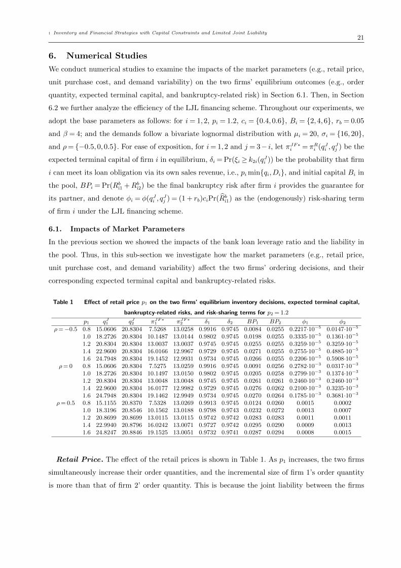
Table 1 Effect of retail price p1 on the two firms’ equilibrium inventory decisions, expected terminal capital,
bankruptcy-related risks, and risk-sharing terms for p2 = 1.2
p1 qJ1 qJ2 πJF∗1 πJF∗2 δ1 δ2 BP1 BP2 φ1 φ2
ρ= −0.5 0.8 15.0606 20.8304 7.5268 13.0258 0.9916 0.9745 0.0084 0.0255 0.2217·10−5 0.0147·10−5
1.0 18.2726 20.8304 10.1487 13.0144 0.9802 0.9745 0.0198 0.0255 0.3335·10−5 0.1361·10−5
1.2 20.8304 20.8304 13.0037 13.0037 0.9745 0.9745 0.0255 0.0255 0.3259·10−5 0.3259·10−5
1.4 22.9600 20.8304 16.0166 12.9967 0.9729 0.9745 0.0271 0.0255 0.2755·10−5 0.4885·10−5
1.6 24.7948 20.8304 19.1452 12.9931 0.9734 0.9745 0.0266 0.0255 0.2206·10−5 0.5908·10−5
ρ= 0 0.8 15.0606 20.8304 7.5275 13.0259 0.9916 0.9745 0.0091 0.0256 0.2782·10−3 0.0317·10−3
1.0 18.2726 20.8304 10.1497 13.0150 0.9802 0.9745 0.0205 0.0258 0.2799·10−3 0.1374·10−3
1.2 20.8304 20.8304 13.0048 13.0048 0.9745 0.9745 0.0261 0.0261 0.2460·10−3 0.2460·10−3
1.4 22.9600 20.8304 16.0177 12.9982 0.9729 0.9745 0.0276 0.0262 0.2100·10−3 0.3235·10−3
1.6 24.7948 20.8304 19.1462 12.9949 0.9734 0.9745 0.0270 0.0264 0.1785·10−3 0.3681·10−3
ρ= 0.5 0.8 15.1155 20.8370 7.5328 13.0269 0.9913 0.9745 0.0124 0.0260 0.0015 0.00021.0 18.3196 20.8546 10.1562 13.0188 0.9798 0.9743 0.0232 0.0272 0.0013 0.00071.2 20.8699 20.8699 13.0115 13.0115 0.9742 0.9742 0.0283 0.0283 0.0011 0.00111.4 22.9940 20.8796 16.0242 13.0071 0.9727 0.9742 0.0295 0.0290 0.0009 0.00131.6 24.8247 20.8846 19.1525 13.0051 0.9732 0.9741 0.0287 0.0294 0.0008 0.0015
Retail Price. The effect of the retail prices is shown in Table 1. As p1 increases, the two firms
simultaneously increase their order quantities, and the incremental size of firm 1’s order quantity
is more than that of firm 2’ order quantity. This is because the joint liability between the firms
: Inventory and Financial Strategies with Capital Constraints and Limited Joint Liability22
is limited, so the direct effect of p1 on firm 2’s strategy and the indirect effect of p1 on firm 2’s
strategy via firm 1’s strategy are relatively low; and a relatively low retail price p1 will significantly
constrain firm 1’s marginal profit and reduce its ability to repay. The two results naturally reduce
the probability δ1 that firm 1 uses its sales revenue and initial capital to repay completely, and
firm 2’s such probability δ2 is very slightly affected. Furthermore, the risk-sharing terms of the
two firms are relatively small and very slightly affected by the retail prices, especially when the
demand correlation is negative. In particular, as firm 1 increases its retail price, such term of firm
2, i.e., φ2, increases, but it is not the case for firm 1. Note that a higher retail price p1 means a
greater marginal profit for firm 1. As a result, firm 1’s revenue also increases and so its expected
terminal capital πJF∗1 increases, whereas firm 2’s expected terminal capital πJF∗2 decreases since
the risk-sharing term of firm 2 becomes larger. This implies that once the two firms choose the
LJL financing scheme, one firm prefers to cooperate with the firm that has a relatively low or high
retail price.
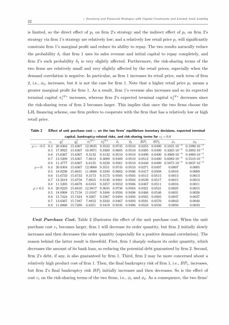
Table 2 Effect of unit purchase cost c1 on the two firms’ equilibrium inventory decisions, expected terminal
capital, bankruptcy-related risks, and risk-sharing terms for c2 = 0.6
c1 qJ1 qJ2 πJF∗1 πJF∗2 δ1 δ2 BP1 BP2 φ1 φ2
ρ= −0.5 0.4 20.8304 15.6367 12.9635 9.3533 0.9745 0.9510 0.0255 0.0490 0.1631·10−4 0.1090·10−4
0.5 17.9925 15.6367 10.9971 9.3309 0.9605 0.9510 0.0395 0.0490 0.3265·10−4 0.2982·10−4
0.6 15.6367 15.6367 9.3132 9.3132 0.9510 0.9510 0.0490 0.0490 0.4969·10−4 0.4969·10−4
0.7 13.5209 15.6367 7.8613 9.3089 0.9489 0.9510 0.0512 0.0490 0.6082·10−4 0.5510·10−4
0.8 11.4777 15.6367 6.6125 9.3229 0.9561 0.9510 0.0440 0.0490 0.5875·10−4 0.3837·10−4
ρ= 0 0.4 20.8304 15.6367 12.9668 9.3551 0.9745 0.9510 0.0271 0.0497 0.0007 0.00050.5 18.0236 15.6631 11.0008 9.3340 0.9602 0.9506 0.0417 0.0508 0.0010 0.00090.6 15.6733 15.6733 9.3173 9.3173 0.9505 0.9505 0.0515 0.0515 0.0013 0.00130.7 13.5618 15.6758 7.8655 9.3130 0.9481 0.9504 0.0539 0.0517 0.0015 0.00130.8 11.5205 15.6678 6.6163 9.3257 0.9552 0.9506 0.0467 0.0511 0.0016 0.0011
ρ= 0.5 0.4 20.9223 15.6810 12.9817 9.3635 0.9738 0.9504 0.0321 0.0521 0.0025 0.00150.5 18.0908 15.7158 11.0187 9.3488 0.9594 0.9498 0.0466 0.0546 0.0031 0.00280.6 15.7424 15.7424 9.3367 9.3367 0.9494 0.9494 0.0565 0.0565 0.0037 0.00370.7 13.6367 15.7487 7.8852 9.3332 0.9467 0.9493 0.0591 0.0570 0.0043 0.00400.8 11.6066 15.7280 6.6351 9.3419 0.9535 0.9496 0.0524 0.0556 0.0050 0.0033
Unit Purchase Cost . Table 2 illustrates the effect of the unit purchase cost. When the unit
purchase cost c1 becomes larger, firm 1 will decrease its order quantity, but firm 2 initially slowly
increases and then decreases the order quantity (especially for a positive demand correlation). The
reason behind the latter result is threefold. First, firm 1 sharply reduces its order quantity, which
decreases the amount of its bank loan, so reducing the potential debt guaranteed by firm 2. Second,
firm 2’s debt, if any, is also guaranteed by firm 1. Third, firm 2 may be more concerned about a
relatively high product cost of firm 1. Then, the final bankruptcy risk of firm 1, i.e., BP1, increases,
but firm 2’s final bankruptcy risk BP2 initially increases and then decreases. So is the effect of
cost c1 on the risk-sharing terms of the two firms, i.e., φ1 and φ2. As a consequence, the two firms’

: Inventory and Financial Strategies with Capital Constraints and Limited Joint Liability23
expected terminal capital decreases in the unit purchase cost c1. In this regard, one firm is a bit
more willing to cooperate with a partner that has a greater advantage in the production cost.
Demand Volatility. We finally illustrate how demand uncertainty influences the two firms’
operations decisions. As shown in Table 3, as σ1 increases, the two firms will simultaneously decrease
their order quantities only for negative demand correlation, which corresponds to low profit mar-
gins. Moreover, the probabilities that the two firms use their own initial capital in the pool and
sales revenues to repay completely decrease because greater demand uncertainty results in a higher
risk. Interestingly, it is observed that the final bankruptcy risks of the two firms will always increase
with firm 1’s demand variability even though their order quantities decrease, since a higher demand
volatility is more concerned by firm 1, which in turn significantly affects firm 2. Consequently, the
two firms’ expected terminal capital decreases in firm 1’s demand uncertainty, which implies that
one firm prefers to cooperating with a firm whose demand variability is lower.
Combining Tables 1, 2, and 3, we further observe that the impact of the characteristics of the
two firms’ products on the risk-sharing terms is significantly small, especially when the demand
correlation is non-positive. This mainly results from the relatively limited liability in the capital
pool. Furthermore, it is interesting to see that the final bankruptcy risks in the case of negative
demand correlation are in general not higher than those in the case of positive demand correlation.
This means that the bank is more willing to support firms whose demand correlation is negative.
Table 3 Effect of demand variability σ1 on the two firms’ equilibrium inventory decisions, expected terminal
capital, bankruptcy-related risks, and risk-sharing terms for σ2 = 16
σ1 qJ1 qJ2 πJF∗1 πJF∗2 δ1 δ2 BP1 BP2 φ1 φ2
ρ= −0.5 12 21.2914 20.8304 14.3656 13.0258 0.9950 0.9745 0.0050 0.0255 0.0034·10−4 0.0038·10−4
14 21.0652 20.8304 13.6521 13.0178 0.9867 0.9745 0.0133 0.0255 0.0130·10−4 0.0140·10−4
16 20.8304 20.8304 13.0037 13.0037 0.9745 0.9745 0.0255 0.0255 0.0326·10−4 0.0326·10−4
18 20.6069 20.8304 12.4180 12.9838 0.9594 0.9745 0.0406 0.0255 0.0633·10−4 0.0581·10−4
20 20.4036 20.8304 11.8901 12.9590 0.9425 0.9745 0.0575 0.0255 0.1045·10−4 0.0876·10−4
ρ= 0 12 21.2914 20.8304 14.3659 13.0260 0.9950 0.9745 0.0053 0.0257 0.0980·10−3 0.1089·10−3
14 21.0652 20.8304 13.6528 13.0182 0.9867 0.9745 0.0137 0.0259 0.1722·10−3 0.1841·10−3
16 20.8304 20.8304 13.0048 13.0048 0.9745 0.9745 0.0261 0.0261 0.2460·10−3 0.2460·10−3
18 20.6069 20.8304 12.4196 12.9859 0.9594 0.9745 0.0413 0.0262 0.3122·10−3 0.2883·10−3
20 20.4036 20.8304 11.8922 12.9622 0.9425 0.9745 0.0584 0.0262 0.3687·10−3 0.3132·10−3
ρ= 0.5 12 21.2914 20.8304 14.3691 13.0273 0.9950 0.9745 0.0069 0.0275 0.0008 0.000914 21.0963 20.8497 13.6578 13.0218 0.9866 0.9744 0.0158 0.0281 0.0010 0.001116 20.8699 20.8699 13.0115 13.0115 0.9742 0.9742 0.0283 0.0283 0.0011 0.001118 20.6535 20.8962 12.4276 12.9964 0.9590 0.9740 0.0437 0.0284 0.0011 0.001020 20.4562 20.9269 11.9013 12.9769 0.9418 0.9738 0.0608 0.0284 0.0012 0.0009
6.2. Efficiency of the LJL Financing Scheme
We now analyze the value of using the LJL financing scheme compared with using the self-financing
scheme, which is illustrated in the following table.We use πJF∗i − πNF∗i (i= 1,2) to represent such

: Inventory and Financial Strategies with Capital Constraints and Limited Joint Liability24
value of the LJL financing scheme. As shown in Table 4, when the bank loan leverage ratio is
relatively low (e.g., β = 2), one of the two firms will use up its credit line to order. In this regard,
as firm 1 has greater liability in the pool, the two firms’ equilibrium order quantities and the
corresponding bankruptcy risks increase. When the ratio is relatively high (e.g., β = 6), the above
result does not hold. These results are consistent with Propositions 3 and 4. Furthermore, as B1
increases, the value of firm 1 under the LJL financing scheme over that under the self-financing
scheme, i.e., πJF∗1 −πNF∗1 , will decrease, and the value of firm 2, i.e., πJF∗2 −πNF∗2 , will decrease for
a relatively low bank loan leverage ratio but increase for a relatively high bank loan leverage ratio
(which is consistent with Proposition 4). This is because higher initial capital of firm 1 means its
constraint on the ordering decision can be more relaxed but leads to a greater loss because firm 1
needs to use its capital in the pool to guarantee for its partner. In addition, in this case the two
firms’ bankruptcy risks, i.e., BP1 and BP2, decrease in firm 1’s liability in the pool.
Table 4 Comparison between the LJL financing scheme and the benchmarking
self-financing scheme for ρ= −0.5 and B2 = 4
B1 β rb qJ1 − qNF∗1 qJ2 − qNF∗2 πJF∗1 −πNF∗1 πJF∗2 −πNF∗2 BP1 BP2
2 2 0.01 5.0000 10.0000 3.0387 2.3174 0.0008 0.01510.05 5.0000 10.0000 2.8737 2.0028 0.0012 0.01970.10 5.0000 10.0000 2.6658 1.6117 0.0017 0.0264
4 0.01 15.0000 11.3277 5.4524 2.2641 0.0548 0.02320.05 15.0000 10.8304 5.1484 1.9166 0.0633 0.02560.10 15.0000 10.2369 4.7724 1.4905 0.0748 0.0285
6 0.01 17.1305 11.3277 1.2780 0.3982 0.3570 0.30890.05 16.6732 10.8304 1.2068 0.3531 0.3701 0.31730.10 16.1290 10.2369 1.1200 0.2997 0.3829 0.3270
4 2 0.01 10.0000 10.0000 2.3052 2.3052 0.0151 0.01510.05 10.0000 10.0000 1.9852 1.9852 0.0197 0.01970.10 10.0000 10.0000 1.5852 1.5852 0.0264 0.0264
4 0.01 11.3277 11.3277 2.3191 2.3191 0.0232 0.02320.05 10.8304 10.8304 1.9869 1.9869 0.0255 0.02550.10 10.2369 10.2369 1.5831 1.5831 0.0283 0.0283
6 0.01 11.3277 11.3277 2.3191 2.3191 0.0232 0.02320.05 10.8304 10.8304 1.9869 1.9869 0.0255 0.02550.10 10.2369 10.2369 1.5831 1.5831 0.0283 0.0283
6 2 0.01 6.0364 10.0000 0.5522 2.3167 0.0021 0.01510.05 5.5138 10.0000 0.2150 2.0020 0.0026 0.01970.10 4.8896 10.0000 -0.1970 1.6108 0.0032 0.0264
4 0.01 6.0364 11.3277 0.5420 2.3409 0.0021 0.02320.05 5.5138 10.8304 0.2072 2.0116 0.0026 0.02550.10 4.8896 10.2369 -0.1998 1.6116 0.0032 0.0283
6 0.01 6.0364 11.3277 0.5420 2.3409 0.0021 0.02320.05 5.5138 10.8304 0.2072 2.0116 0.0026 0.02550.10 4.8896 10.2369 -0.1998 1.6116 0.0032 0.0283
We also observe that as the bank loan leverage ratio increases, the two firms will over-invest
more in their ordering. Thus, the bankruptcy risks faced by them, i.e., BP1 and BP2, will also
increase. This is consistent with the results in Proposition 5. Interestingly, we also see that a higher

: Inventory and Financial Strategies with Capital Constraints and Limited Joint Liability25
bank loan leverage ratio, which means greater credit lines for the two firms, does not always bring
more benefit to the firms (e.g., firm 1). Also, even when the two firms have equal proportions of
the liability in the pool, the values of the two firms adopting the LJL financing scheme do not
increase with the bank loan leverage ratio simultaneously. In sum, we see that increasing the credit
lines is not necessarily beneficial to the two firms simultaneously. Moreover, the numerical results
also show that when the initial capital is at a relatively high level (e.g., B1 ≥ 6) and the interest
rate is considerable (e.g., rb ≥ 0.1), the value of firm 1 using the LJL financing is negative, which
means that adopting the no-finance scheme is preferable. This holds for the case when the interest
rate is relatively high, even though the two firms are very financially constrained (e.g., 1≤ rb < 2,
1<β ≤ 1.5). These results are consistent with Proposition 6.
7. Discussions7.1. Endogenizing the Bank-loan Leverage Ratio and the Interest Rate
So far we have analyzed the firms’ operations and financial decisions for exogenously given bank
loan leverage ratio and interest rate. However, in anticipation of the best responses of the two firms
in Section 3.2, the bank needs to determine the bank loan leverage ratio β (or credit line) and
interest rate rb. We refer to this as the bank’s problem, which we consider in this section. In line
with the literature (e.g., Kouvelis and Zhao 2012, Chod 2017, Yang and Birge 2017), we assume
that the bank loan market is competitive, which means that the loan terms (β and rb) are offered
at which the bank expects to make zero profit. Since under the LJL financing scheme, the two
firms should bear each other’s bankruptcy risk, at the end of the selling period, the bank’s has
three possible outcomes for its terminal revenue as follows: (a) it completely recoups its loans to
the two firms, (b) it completely recoups the loan to one firm but only partially recoups the loan
to the other firm, and (c) it fails to recoup the loans to the two firms. We can classify the three
outcomes into the following four regions:
Ω1 =ξ≥ 0 : ξi ≤ k1i(qi), ξj ≤ k1j(qj), piξi + pjξj ≤ pikbi(qi, qj)
,
Ω2 =ξ≥ 0 : ξi ≤
pik2i(qi)−Bjpi
, ξj ≥ k1j(qj),
Ω3 =ξ≥ 0 : ξj ≤
pjk2j(qj)−Bipj
, ξi ≥ k1i(qi),
Ω4 =ξ≥ 0 : piξi + pjξj ≥ pikbi(qi, qj), ξi ≥
pik2i(qi)−Bjpi
, ξj ≥pjk2j(qj)−Bi
pj
,
where (qi, qj) = (qJi , qJj ). In Appendix B, we use Figure 2 to illustrate the four regions above, and
state their event meanings. Based on the above discussion, then we express the expected terminal
revenue of the bank as follows:
ΠB(β, rb) =Pr(Ω1)E (piξi + pjξj +Bi +Bj|Ω1) + Pr(Ω2)E (pjk1j(qj) + piξi +Bi +Bj|Ω2)
+ Pr(Ω3)E (pik1i(qi) + pjξj +Bi +Bj|Ω3) + Pr(Ω4)E (pik1i(qi) + pjk1j(qj)|Ω4) , (9)

: Inventory and Financial Strategies with Capital Constraints and Limited Joint Liability26
where (qi, qj) = (qJi , qJj ) for i = 1,2 and j = 3 − i. The optimal bank loan leverage ratio β∗ and
interest rate r∗b , with 0≤ rb ≤mini=1,2pi/ci− 1 and β > 1, must satisfy the following equation
ΠB(β, rb) = (1 + rf )(ciqi + cjqj). (10)
It follows from Proposition 2 that the bank’s expected terminal revenue ΠB(β, rb) is closely
affected by the bank loan leverage ratio if and only if when β ≤maxi=1,2
ciqi /Bi. However, it is some-
what complicated to analytically solve Equation (10), so we conduct numerical studies to further
analyze the bank’s problem. As shown in Table 5, an interesting observation is that the relationship
Table 5 The equilibrium outcomes for endogenized bank-loan leverage ratio and interest rate
for rf = 0.03 and σi = 20, i= 1,2
(a) ρ= −0.5
B1 (β∗, r∗b ) ΠB(β∗, r∗b ) qJ1 qJ2 πJF∗1 πJF∗2 πNF∗1 πNF∗2 k21 k22 kbi2 (2,0.0303) 12.3600 6.6667 13.3333 5.3575 8.6557 3.9574 7.5256 1.7677 3.5354 5.3031
(3,0.0310) 15.2250 10.0000 14.6360 6.2546 8.6356 3.9574 7.5256 3.4883 4.2115 7.6997(4,0.0310) 17.2930 13.3333 14.6490 6.7242 8.4757 3.9574 7.5256 5.2081 4.2198 9.4280(6,0.0310) 19.1845 16.3868 14.6561 6.8477 8.2134 3.9574 7.5256 6.8047 4.2433 11.0480
4 (2,0.0300) 16.4800 13.3333 13.3333 8.6076 8.6076 7.5256 7.5256 3.5334 3.5334 7.0668(3,0.0301) 18.4115 14.8960 14.8960 8.5817 8.5817 7.5256 7.5256 4.3387 4.3387 8.6774(4,0.0301) 18.4114 14.8960 14.8960 8.5817 8.5817 7.5256 7.5256 4.3387 4.3387 8.6774(6,0.0301) 18.4114 14.8960 14.8960 8.5817 8.5817 7.5256 7.5256 4.3387 4.3387 8.6774
6 (2,0.0300) 16.8187 13.8814 13.3333 10.5635 8.6540 10.4775 7.5256 2.1489 3.5333 5.6823(3,0.0300) 17.7915 13.8814 14.9074 10.5027 8.6883 10.4775 7.5256 2.1489 4.3440 6.4930(4,0.0300) 17.7915 13.8814 14.9074 10.5027 8.6883 10.4775 7.5256 2.1489 4.3440 6.4930(6,0.0300) 17.7915 13.8814 14.9074 10.5027 8.6883 10.4775 7.5256 2.1489 4.3440 6.4930
8 (2,0.0300) 16.7105 13.7063 13.3333 12.5573 8.6609 12.8476 7.5256 0.3921 3.5333 3.9254(3,0.0300) 17.6833 13.7063 14.9074 12.4964 8.6953 12.8476 7.5256 0.3921 4.3440 4.7361(4,0.0300) 17.6833 13.7063 14.9074 12.4964 8.6953 12.8476 7.5256 0.3921 4.3440 4.7361(6,0.0300) 17.6833 13.7063 14.9074 12.4964 8.6953 12.8476 7.5256 0.3921 4.3440 4.7361
(b) ρ= 0.5
2 (2,0.0310) 12.3600 6.6667 13.3333 5.3614 8.6518 3.9574 7.5256 1.7700 3.5400 5.3100(3,0.0343) 15.1479 10.0000 14.5111 6.2650 8.6296 3.9574 7.5256 3.5050 4.1713 7.6763(4,0.0390) 17.2242 13.3333 14.5375 6.7124 8.4915 3.9574 7.5256 5.2600 4.2189 9.4788(6,0.0451) 18.8721 15.9278 14.6095 6.8028 8.3032 3.9574 7.5256 6.6567 4.3011 10.9578
4 (2,0.0326) 16.4800 13.3333 13.3333 8.6076 8.6076 7.5256 7.5256 3.5504 3.5504 7.1007(3,0.0352) 18.0950 14.6400 14.6400 8.5927 8.5927 7.5256 7.5256 4.2442 4.2442 8.4884(4,0.0352) 18.0950 14.6400 14.6400 8.5927 8.5927 7.5256 7.5256 4.2442 4.2442 8.4884(6,0.0352) 18.0950 14.6400 14.6400 8.5927 8.5927 7.5256 7.5256 4.2442 4.2442 8.4884
6 (2,0.0309) 16.8175 13.8795 13.3333 10.5671 8.6504 10.4775 7.5256 2.1540 3.5391 5.6931(3,0.0315) 17.7000 13.9057 14.7350 10.5194 8.6792 10.4775 7.5256 2.1719 4.2662 6.4381(4,0.0315) 17.7000 13.9057 14.7350 10.5194 8.6792 10.4775 7.5256 2.1719 4.2662 6.4381(6,0.0315) 17.7000 13.9057 14.7350 10.5194 8.6792 10.4775 7.5256 2.1719 4.2662 6.4381
8 (2,0.0301) 16.7105 13.7063 13.3333 12.5582 8.6599 12.8476 7.5256 0.3929 3.5341 3.9271(3,0.0303) 17.6679 13.7403 14.8486 12.5018 8.6926 12.8476 7.5256 0.4118 4.3160 4.7278(4,0.0303) 17.6679 13.7403 14.8486 12.5018 8.6926 12.8476 7.5256 0.4118 4.3160 4.7278(6,0.0303) 17.6679 13.7403 14.8486 12.5018 8.6926 12.8476 7.5256 0.4118 4.3160 4.7278
between the optimal bank loan leverage ratio β∗ and interest rate r∗b satisfying Equation (10) is
always non-negative. That is, as the bank offers a higher leverage ratio to its firms, it correspond-
ingly increases the interest rate slightly in order to control the risks from the increasing order
: Inventory and Financial Strategies with Capital Constraints and Limited Joint Liability27
quantities of the two firms. As shown in the previous section, the final bankruptcy risks in the case
of negative demand correlation (e.g., ρ = −0.5) are smaller, relative to those in the other cases.
This is true for the case of endogenized bank-loan leverage ratio and interest rate. As a result,
comparing Table 5(a) and (b), the optimal interest rate when the demand correlation is negative
is lower than that when the demand correlation is positive. Moreover, since the final bankruptcy
risks are very low, the bank will set the optimal interest rate closer to the risk-free rate, while
generating a slightly higher expected revenue in the case of negative demand correlation.
Table 5 also illustrates that as the capital committed by the two firms to the pool increases,
the bank may initially increase and then decrease (rather than always increases) its interest rate,
especially in the case of positive demand correlation. For the first half part, this is because in this
case, at least one firm will use up all the credit line to order, so its order quantity linearly increases
with its own capital in the pool. This results in a larger increase in its effective bankruptcy risk. To
reduce the potential loss from this, it is optimal for the bank to slightly increase the interest rate.
As a result, the bank’s expected terminal revenue may also initially increase and then decrease.
In addition, we observe that the two firms’ equilibrium order quantities, so their expected ter-
minal capital, are not always simultaneously increasing in the capital in the pool. In particular,
when the bank loan leverage ratio is relatively high (such that the two firms can order up to the
non-trivial interior equilibrium level), as one firm’s capital in the pool increases, its order quantity
and the corresponding bankruptcy risk decrease, but it is not the case for the other firm. However,
the firms’ expected terminal capital will always increase with the initial capital, which is consistent
with Proposition 3. When the bank loan leverage ratio is low, there is at least one firm (e.g., firm 1)
using up all its credit line to order and the impacts of the capital in the pool on the firms’ expected
terminal capital are consistent with Proposition 4. Moreover, Table 5 shows that our main insights
from Proposition 5 and Corollary 2 remain unchanged.
It is evident from Table 5 that our numerical results are also consistent with Theorem 2. When
the bank-loan leverage ratio is relatively high (e.g., β ≥ 3), which satisfies β > pipi−ci
= 2, the optimal
interest rate charged by the bank satisfies 0< rb ≤ β−1β
pici− 1. Correspondingly, the values of the
firms using LJL financing scheme are positive if the capital in the pool is low (e.g., B1 ≤ 6), so
both firms prefer the LJL financing scheme; otherwise (e.g., B1 = 8), there is at least one firm
receiving a negative value of using the LJL financing scheme, so cooperation in financing cannot
be achieved. In addition, when the bank sets a sufficiently low leverage ratio (e.g., 1<β ≤ 2), the
resulting interest rate will satisfy (β−1)pici−βrb ≤ β−1. Accordingly, the value of at least one firm
using the LJL financing scheme is negative (especially when the unit product costs are relatively
high), so the self-financing scheme becomes the equilibrium financing scheme.

: Inventory and Financial Strategies with Capital Constraints and Limited Joint Liability28
7.2. Generalizing the Allocation of Initial Capital
We now consider the case where the firms have the opportunity to allocate their initial capital.
That is, each firm can commit a portion of its own initial capital to the joint capital pool to
obtain external financing, while using the remaining initial capital to self-finance inventory. Note
that although having the remaining initial capital to self-finance inventory can reduce their total
financing costs, their credit lines may be more constrained (related to the case in Section 3.2). In
this regard, the firms need to make a trade-off between the financing cost and potential loss from
the limited credit line. Then, it is natural to ask the question: Under what condition is it that
committing a part of the initial capital to the pool is always better?
To answer this question, following the practice in the Introduction, we consider a game among
the three players, i.e., the two firms and the bank, as follows: Prior to the selling season, the two
firms simultaneously decide to commit the amount of liability (denoted by Ti, i= 1,2), from their
own initial capital Bi, to the capital pool, i.e., Ti ≤ Bi. Next, the bank makes its decisions, i.e.,
setting the bank loan leverage ratio β and interest rate rb, with the expectation that it makes zero
profit. Upon knowing the bank’s decisions, the two firms simultaneously place their order quantities
by borrowing a loan ciqi− (Bi− Ti), within the credit line plus the remaining initial capital, i.e.,
βTi +Bi−Ti. The remaining events are the same as those in the second and third steps described
in Section 3. Similar to Section 3.2, we formulate the expected terminal capital of firm i, for i= 1,2
and j = 3− i, as follows:
πAi (qi,qj,T) =Eξi,ξj
[piminqi, ξi− (1 + rb)(ciqi +Ti−Bi)]+
+[Ti− ((1 + rb)(ciqi +Ti−Bi)− piξi)+− ((1 + rb)(cjqj +Tj −Bj)− pjξj −Tj)+
]+, (11)
where T = (Ti, Tj) and the superscript A denotes the case of endogenized allocation of the initial
capital. Next we solve the problems faced by the two firms and the bank using the backward
approach. First, given the firms’ liability, i.e., Ti, i= 1,2, and the bank’s decisions β and rb, each
firm i chooses its order quantity qi to maximize its expected terminal capital. That is,
qAi (β, rb,T) = arg maxBi/ci≤qi≤((β−1)Ti+Bi)/ci
πJFi (qi, qj,T), i= 1,2, j = 3− i. (12)
Second, based on the firms’ best order quantities above, we find the optimal leverage ratio βA(T)
and interest rate rAb (T) of the bank by solving the following equation
ΠB(β, rb,T) = (1 + rf )[(ciqAi (β, rb,T) +Ti−Bi) + (cjq
Aj (β, rb,T) +Tj −Bj)], (13)
where ΠB(β, rb,T) is the same as that in Equation (9) by replacing Bi with Ti and ciqi with
ciqAi (β, rb,T)+Ti−Bi. Third, based on the solutions of Equations (12) and (13), each firm i chooses
its liability Ti to commit to the capital pool. That is,
TAi = arg maxTi≤Bi
πJFi (qAi (βA(T), rAb (T),T), qAi (βA(T), rAb (T),T),T), i= 1,2, j = 3− i. (14)
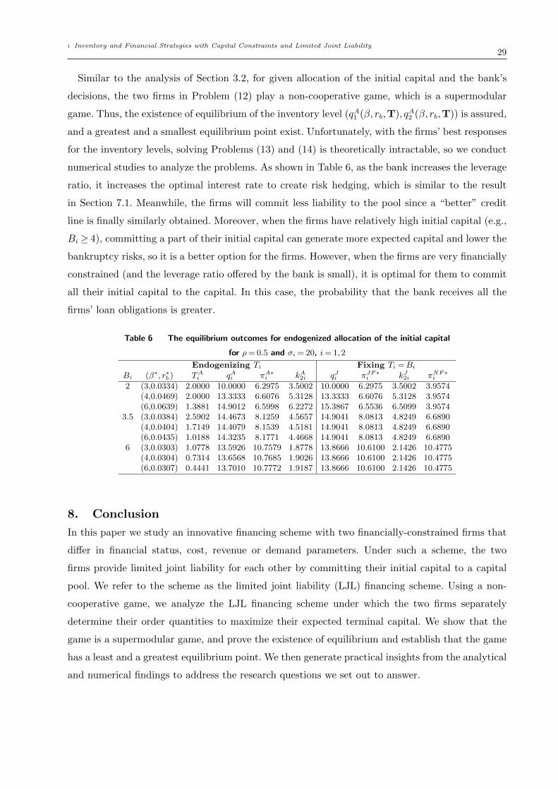
: Inventory and Financial Strategies with Capital Constraints and Limited Joint Liability29
Similar to the analysis of Section 3.2, for given allocation of the initial capital and the bank’s
decisions, the two firms in Problem (12) play a non-cooperative game, which is a supermodular
game. Thus, the existence of equilibrium of the inventory level (qA1 (β, rb,T), qA2 (β, rb,T)) is assured,
and a greatest and a smallest equilibrium point exist. Unfortunately, with the firms’ best responses
for the inventory levels, solving Problems (13) and (14) is theoretically intractable, so we conduct
numerical studies to analyze the problems. As shown in Table 6, as the bank increases the leverage
ratio, it increases the optimal interest rate to create risk hedging, which is similar to the result
in Section 7.1. Meanwhile, the firms will commit less liability to the pool since a “better” credit
line is finally similarly obtained. Moreover, when the firms have relatively high initial capital (e.g.,
Bi ≥ 4), committing a part of their initial capital can generate more expected capital and lower the
bankruptcy risks, so it is a better option for the firms. However, when the firms are very financially
constrained (and the leverage ratio offered by the bank is small), it is optimal for them to commit
all their initial capital to the capital. In this case, the probability that the bank receives all the
firms’ loan obligations is greater.
Table 6 The equilibrium outcomes for endogenized allocation of the initial capital
for ρ= 0.5 and σi = 20, i= 1,2
Endogenizing Ti Fixing Ti =BiBi (β∗, r∗b ) TAi qAi πA∗i kA2i qJi πJF∗i kJ2i πNF∗i
2 (3,0.0334) 2.0000 10.0000 6.2975 3.5002 10.0000 6.2975 3.5002 3.9574(4,0.0469) 2.0000 13.3333 6.6076 5.3128 13.3333 6.6076 5.3128 3.9574(6,0.0639) 1.3881 14.9012 6.5998 6.2272 15.3867 6.5536 6.5099 3.9574
3.5 (3,0.0384) 2.5902 14.4673 8.1259 4.5657 14.9041 8.0813 4.8249 6.6890(4,0.0404) 1.7149 14.4079 8.1539 4.5181 14.9041 8.0813 4.8249 6.6890(6,0.0435) 1.0188 14.3235 8.1771 4.4668 14.9041 8.0813 4.8249 6.6890
6 (3,0.0303) 1.0778 13.5926 10.7579 1.8778 13.8666 10.6100 2.1426 10.4775(4,0.0304) 0.7314 13.6568 10.7685 1.9026 13.8666 10.6100 2.1426 10.4775(6,0.0307) 0.4441 13.7010 10.7772 1.9187 13.8666 10.6100 2.1426 10.4775
8. Conclusion
In this paper we study an innovative financing scheme with two financially-constrained firms that
differ in financial status, cost, revenue or demand parameters. Under such a scheme, the two
firms provide limited joint liability for each other by committing their initial capital to a capital
pool. We refer to the scheme as the limited joint liability (LJL) financing scheme. Using a non-
cooperative game, we analyze the LJL financing scheme under which the two firms separately
determine their order quantities to maximize their expected terminal capital. We show that the
game is a supermodular game, and prove the existence of equilibrium and establish that the game
has a least and a greatest equilibrium point. We then generate practical insights from the analytical
and numerical findings to address the research questions we set out to answer.
: Inventory and Financial Strategies with Capital Constraints and Limited Joint Liability30
We find that using the LJL financing scheme does not always dominate the self-finance scheme,
especially when the bank loan leverage ratio is relatively small and the interest rate is high, or at
least one firm is not extremely-financially constrained. Under the LJL financing scheme, the two
firms’ strategies are complementary. Moreover, we analyze the impacts of each firm’s liability in
the pool and the bank-loan leverage ratio on the two firms’ equilibrium inventory levels, expected
terminal capital, and bankruptcy-related risks. Interestingly, we show that when a firm that uses
up all its credit line to order, it has a larger proportion of the liability in the pool, the two firms
will borrow more bank loans, and the expected terminal capital of the other firm becomes less,
i.e., it may be more harmful to the other firm. In addition, it is somewhat surprising that a higher
bank-loan leverage ratio provided by the bank cannot always simultaneously improve the two firms’
performance because the firms under the LJL financing scheme mutually reinforce one another.
We also find that the bank in general prefers negative correlation between the firms’ demands
because such demands correlation yields lower final bankruptcy risks from the firms. Due to the
characteristic of the LJL financing scheme, varying a market parameter of each firm weakly affects
its partner’s strategy, so the expected cash level. Furthermore, when the bank loan market is
competitive, the interest rate and bank-loan leverage ratio are mutually affected as the bank seeks
to create risk hedging; meanwhile, the capital committed to the pool does not induce the bank to
always reduce the interest rate. In particular, if the firms are very financially constrained, which
means that they use up all their credit lines to order, increasing the interest rate can mitigate
the risks from the linearly increasing order quantities of the firms. Otherwise, as they commit
more initial capital to the pool, their equilibrium order quantities will remain unchanged but the
corresponding final bankruptcy risks will decrease. As a consequence, the bank will decrease the
interest rate. Last but not least, our findings also demonstrate that committing all the initial capital
to the capital pool is not necessarily an inferior choice for the firms that are relatively financially
constrained (especially for a relatively small bank-loan leverage ratio).
While our study is an initial attempt to explore the role of joint liability in capital-constrained
firms’ operational decisions and performance, future research may extend our work in several
directions. Considering the case where the suppliers strategically set the wholesale prices is of
interest, which represents the first step towards studying the (limited) joint liability financing
scheme in a supply chain. Another interesting research direction is to consider multiple firms under
the LJL financing scheme and study how each firm in the joint-liability group should bear the
bankruptcy risks of the other firms. Recall that we assume that the firms considered in this paper
are credit-worthy. As argued in the related literature on group lending (e.g., Chowdhury 2005),
a moral hazard between the group-lending firms and the bank exists, so incorporating this factor
into our model will be another interesting and challenging topic for future research.
: Inventory and Financial Strategies with Capital Constraints and Limited Joint Liability31
References
Babich, V., M.J. Sobel. 2004. Pre-IPO operational and financial decisions. Management Science 50(7): 935-
948.
Bhole, B., S. Ogden. 2010. Group lending and individual lending with strategic default. Journal of Develop-
ment Economics 91(2): 348-363.
Buzacott, J.A., R. Zhang. 2004. Inventory management with asset-based financing. Management Science
24(9): 1274-1292.
Cachon, G.P., S. Netessine. 2004. Game theory in supply chain analysis. D. Simchi-Levi, S.D. Wu, and M.
Shen eds., The eBusiness Era, Kluwer.
Cai, G.S., X. Chen, Z. Xiao. 2014. The roles of bank and trade credits: Theoretical analysis and empirical
evidence. Production and Operations Management 23(4): 583-598.
Caldentey, R., X. Chen. 2010. The role of financial services in procurement contracts. P. Kouvelis, O. Boy-
abatli, L. Dong, R. Li, eds., Handbook of Integrated Risk Management in Global Supply Chains, John
Wiley & Sons, Inc., 289-326.
Chao, X., J. Chen, S. Wang. 2008. Dynamic inventory management with cash flow constraints. Naval Research
Logistics 55(8): 758-768.
Chen, X., G. Cai, J.S. Song. 2018. The cash flow advantages of 3PLs as supply chain orches-
trators. Manufacturing & Service Operations Management. Forthcoming. Available at SSRN:
https://ssrn.com/abstract=2679357 or http://dx.doi.org/10.2139/ssrn.2679357.
Chen, Y.B. 2016. Essays on supply chain finance. Ph.D. Thesis, University of Minnesota, Twin Cities.
Chod, J. 2017. Inventory, risk shifting, and trade credit. Management Science 63(10): 3207-3225.
Chowdhury, P. 2005. Group-lending: Sequential financing, lender monitoring and joint liability. Journal of
Development Economics 77(2): 415-439.
Cooper, R., A. John. 1988. Coordinating coordination failures in Keynesian models. The Quarterly Journal
of Economics 103(3): 441-463.
Dada, M., Q. Hu. 2008. Financing newsvendor inventory. Operations Research Letters 36(5): 569-573.
Deng, S., C. Gu, S. Cai, Y. Li. 2018. Financing multiple heterogeneous suppliers in assembly systems: Buyer
finance vs. bank finance. Manufacturing & Service Operations Management 20(1): 53-69.
Ghatak, M. 1999. Group lending, local information and peer selection. Journal of Development Economics
60(1): 27-50.
Ghatak, M. 2000. Screening by the company you keep: joint liability lending and the peer selection effect.
Economic Journal 110(456): 601-631.
Gong, X.T., X. Chao, D. Simchi-Levi. 2014. Dynamic inventory control with limited capital and short-term
financing. Naval Research Logistics 61(3): 184-201.

: Inventory and Financial Strategies with Capital Constraints and Limited Joint Liability32
Gupta, D., L. Wang. 2009. A stochastic inventory model with trade credit. Manufacturing & Service Oper-
ations Management 11(1): 4-18.
Jing, B., X. Chen, G. Cai. 2012. Equilibrium financing in a distribution channel with capital constraint.
Production and Operations Management 21(6): 1090-1101.
Kouvelis, P., W. Zhao. 2011. The newsvendor problem and price-only contract when bankruptcy costs exist.
Production and Operations Management 20(6): 921-936.
Kouvelis, P., W. Zhao. 2012. Financing the newsvendor: Supplier vs. bank, and the structure of optimal
trade credit contracts. Operations Research 60(3): 566-580.
Kouvelis, P., W. Zhao. 2016. Supply chain contract design under financial constraints and bankruptcy costs.
Management Science 62(8): 2341-2357.
Kouvelis, P., W. Zhao. 2018. Who should finance the supply chain? Impact of credit ratings on supply chain
decisions. Manufacturing & Service Operations Management 20(1): 19-35.
Lai, G., L.G. Debo, K. Sycara. 2009. Sharing inventory risk in supply chain: The implication of financial
constraint. Omega 37(4): 811-825.
Li, L., M. Shubik, M.J. Sobel. 2013. Control of dividends, capital subscriptions, and physical inventories.
Management Science 59(5): 1107-1124.
Lippman, S., K. McCardle. 1997. The competitive newsboy. Operations Research 45(1): 54-65.
Luo, W., K. Shang. 2015. Joint inventory and cash management for multidivisional supply chains. Operations
Research 63(5): 1098-1116.
Modigliani, F., M.H. Miller. 1958. The cost of capital, corporation finance and the theory of investment. The
American Economic Review 48(3): 261-297.
Rezaei, B., S. Dasu, R. Ahmadi. 2017. Optimal group size in joint liability contracts. Decision Analysis
14(3): 204-225.
Stiglitz, J. 1990. Peer monitoring and credit markets. World Bank Economic Review 4(3): 351-366.
Tang, C.S., J. Wu, S.A. Yang. 2018. Sourcing from suppliers with financial constraints and performance risk.
Manufacturing & Service Operations Management 20(1): 70-84.
Topkis, D.M. 1998. Supermodularity and Complementarity. Princeton University Press.
Tunca, T.I., W. Zhu. 2017. Buyer intermediation in supplier finance. Management Science, ePub ahead of
print November 2, https://doi .org/10.1287/mnsc.2017.2863.
Vandenberg, P. 2003. Adapting to the financial landscape: Evidence from small firms in Nairobi. World
Development 31(11): 1829-1843.
Wu, A.A. 2017. supportive pricing model for suppliers with purchase order financing. International Journal
of Production Research 55(19): 5632-5646.
: Inventory and Financial Strategies with Capital Constraints and Limited Joint Liability33
Wydick, B. 2001. Group lending under dynamic incentives as a borrower discipline device. Review of Devel-
opment Economics 5(3): 406-420.
Xu, X., J.R. Birge. 2004. Joint production and financing decisions: modeling and analysis. Available at
SSRN: http://ssrn.com/paper=652562.
Xu, X., J.R. Birge. 2006. Equity valuation, production, and financial planning: A stochastic programming
approach. Naval Research Logistics 53(7): 641-655.
Xu, X., J.R. Birge. 2008. Operational decisions, capital structure, and managerial compensation: a news
vendor perspective. The Engineering Economist 53(3): 173-196.
Yang, S.A., J.R. Birge. 2011. Trade credit in supply chains: Multiple creditors and priority rules. Available
at SSRN: https://ssrn.com/abstract=1840663.
Yang, S.A., J.R. Birge. 2017. Trade credit, risk sharing, and inventory financing portfolios. Management
Science, ePub ahead of print August 18, https://doi.org/10.1287/mnsc.2017.2799.
Zhou, J., H. Groenevelt. 2008. Impacts of financial collaboration in a three-party supply chain. Working
Paper, The Simon School, University of Rochester, Rochester, NY.

: Inventory and Financial Strategies with Capital Constraints and Limited Joint Liability34
Appendix A: Notation
Table 7 Notation (i= 1,2)
Bi Firm i’s initial capitalpi Retail price per unit product of firm ici Purchase cost per unit product of firm iqi Firm i’s order quantity (a decision variable)rb Interest rate on the bank loan under the LJL financing scheme, where ci(1 + rb)≤ pirf Risk-free interest rateβ Bank loan leverage ratio set by the bank depending on the amount of the initial
capital in the capital poolk1i(qi) Firm i’s breakeven threshold, i.e., the minimum demand for firm i’s product to meet
its loan obligation with its realized sales revenuek2i(qi) Firm i’s effective bankruptcy threshold, i.e., the minimum demand for firm i’s
product to meet its loan obligation with all its available capital in the poolkbi(qi, qj) Firm i’s eventual potential bankruptcy threshold, i.e., the minimum demand for a breakeven
firm i’s product to finally survive when it shoulders the liability of a worst-case firm jξi,ξ Random demand for firm i’s product and the demands vector, respectivelyfξ(·, ·), Fξ(·, ·) Probability density and cumulative distribution functions of the positive
vector ξ, respectivelyfξi(·), Fξi(·) The marginal cumulative and probability distribution functions of ξ in terms of
random variable ξi, respectivelyFξi(·) The complementary marginal cumulative distribution function of the demand ξiφ(qi, q3−i) Risk-sharing term of firm i under the LJL financing schemeπNFi , πJFi Firm i’s expected terminal capital under the no-financing and LJL financing schemes,
respectively
Appendix B: More Details of Sub-regions Defined in Sections 3.2 and7.1
In Section 3.2, according to Figure 1, the six sub-regions can be further described in detail as:
Rai1 =
ξ≥ 0 : ξi ≤ k1i(qi), ξj ≤ k2j(qj),and piξi + pjξj ≥ pikbi(qi, qj)
,
Rbi1 =
ξ≥ 0 : ξi ≤ k1i(qi), ξj ≤ k2j(qj),and piξi + pjξj < pikbi(qi, qj)
,
Rai2 =
ξ≥ 0 : k2i(qi)≤ ξi <k1i(qi), ξj ≥ k2j(qj)
,
Rbi2 =
ξ≥ 0 : ξi <k2i(qi), ξj ≥ k2j(qj)
,
Rai3 =
ξ≥ 0 : ξi ≥ k1i(qi), ξj ≤ k2j(qj)
,
Rai4 =
ξ≥ 0 : ξi ≥ k1i(qi), ξj ≥ k2j(qj)
.
Furthermore, we state the event meanings of these sub-regions as follows:
• In sub-regions Rbi1 and Rb
i2, firm i does not sell all its ordered product, and either does not
have enough sales revenue and initial capital to meet its loan obligation, or does not have enough
remaining initial capital in the pool after repaying its loan to cover the debt of (bankrupt) firm j.
Thus, firm i’s terminal capital is 0;

: Inventory and Financial Strategies with Capital Constraints and Limited Joint Liability35
• In sub-region Rai1, firm i’s sales revenue is not enough to meet its own loan obligation, but its
initial capital in the pool can cover the remaining debt, and firm i’s remaining initial capital can
also cover firm j’s remaining debt. In this case, firm i’s terminal capital is Bi− (1 + rb)ciqi +piξi−
(1 + rb)cjqj + pjξj +Bj;
• In sub-region Rai2, firm j has enough sales revenue and initial capital in the pool to repay its
loan, and firm i can use its initial capital to cover its remaining debt even though firm i does not
have enough sales revenue to repay its loan. Thus, firm i’s terminal capital is Bi− (1+rb)ciqi+piξi;
• In sub-region Rai3, firm i has enough sales revenue to meet its loan obligation. In this case,
firm i’s terminal capital is piminqi, ξi− (1 + rb)ciqi + (Bi− (1 + rb)cjqj + pjξj +Bj))+;
• In sub-region Rai4, the two firms simultaneously have enough sales revenues and initial capital
to cover their debts. Thus, firm i’s terminal capital is piminqi, ξi− (1 + rb)ciqi +Bi.
In Section 7.1, we use Figure 2 to depict the four regions of (ξi, ξj), whose meanings we state as
follows:
ix
jx
( , )bi i j
k q q
( , )bj j i
k q q
2( )
i ik q
2( )
j jk q
1( )
i ik q
4W
0
2( )
j j j i
j
p k q B
p
-
2( )
i i i j
i
p k q B
p
-
1( )
j jk q
2W
3W
1W
Figure 2 Partition of the demand pair (ξi, ξj).
• In sub-region Ω1, the two firms do not have enough sales revenues to completely repay their
loans and their initial capital in the pool cannot pay their remaining debts. In this case, the bank
receives the two firms’ sales revenues and initial capital in the pool, i.e., piξi + pjξj +Bi +Bj;
• In sub-region Ω2, firm j’s sales revenue can completely repay its loan, but firm i’s sales revenue
and initial capital in the pool are not enough to repay its loan, and firm j’s initial capital in the
pool can pay firm i’s remaining debt. Thus, the bank receives (1 + rb)cjqj + piξi +Bi +Bj;
: Inventory and Financial Strategies with Capital Constraints and Limited Joint Liability36
• In sub-region Ω3, firm i’s sales revenue can completely repay its loan, but firm j’s sales revenue
and initial capital in the pool are not enough to repay its loan, and firm i’s initial capital in the
pool can pay firm j’s remaining debt. Thus, the bank receives (1 + rb)ciqi + pjξj +Bi +Bj;
• In sub-region Ω4, the two firms have enough sales revenues and initial capital to pay their own
loans. In this case, the bank’s terminal revenue is (1 + rb)(ciqi + cjqj).
Appendix C: Proofs
Proof of Lemma 1: By the concavity of πNFi (qi), this result is easy to show, so we omit the proof
here.
Proof of Lemma 2: By Lemma 1, when Bi < ciF−1ξi
(c′ipi
), firm i’s optimal expected terminal capital
is πNF∗i = pi(Bi/ci−
∫∞0
∫ Bi/ci0
Fξ(x, y)dxdy). Thus, we have
dπNF∗i
dBi=pici
(1−∫ ∞
0
Fξ(Bi/ci, y)dxd) =piciFξi(Bi/ci),
which is positive and not less than 1 since Bi < ciF−1ξi
(c′ipi
)< ciF−1ξi
( cipi
). In addition, it follows thatd2πNF∗i
dB2i
=− pic2ifξi(Bi/ci)< 0. Obviously,
dπNF∗idBi
is continuous in Bi.
Proof of Lemma 4: It is straightforward to derive the results in Lemma 4 by the definition of
φ(qi, qj).
Proof of Proposition 1: Notice that the first and second terms on the right-hand-side of Equation
(6) are not associated with the decision variable qj. So taking the first-order partial derivatives of
the two sides of Equation (6) with respect to qj yields∂2πJFi (qi,qj)
∂qj∂qi=
∂φ(qi,qj)
∂qj. To prove the increasing-
difference property of πJFi (qi, qj), it suffices to show that∂φ(qi,qj)
∂qj≥ 0. From the definition of Rb
i1 in
Equation (6), φ(qi, qj) = (1 + rb)ciPr(Rbi1). Then, when qj ≥
Bi+Bj(1+rb)cj
, we have
Rbi1 =
ξ ≥ 0 : k2i(qi)< ξi ≤ k1i(qi),and piξi + pjξj < pikbi(qi, qj)
.
This directly yields
∂φ(qi, qj)
∂qj= (1 + rb)ci
∂Pr(Rbi1)
∂qj
=(1 + rb)
2cicjpj
∫ k1i(qi)
k2i(qi)
fξ
(x,pikbi(qi, qj)− pix
pj
)dx> 0,
where fξ(x, y)≥ 0 for any (x, y)≥ 0. Similarly, when qj <Bi+Bj
(1+rb)cj, we have
∂φ(qi, qj)
∂qj=
(1 + rb)2cicj
pj
∫ kbi(qi,qj)
k2i(qi)
fξ
(x,pikbi(qi, qj)− pix
pj
)dx> 0.
Note that from Lemma 4(i),∂φ(qi,qj)
∂qjis continuous at the point qj =
Bi+Bj(1+rb)cj
since, at this point,
k1i(qi) = kbi(qi, qj), i.e., for any qj ≥ 0,∂φ(qi,qj)
∂qj≥ 0. In addition, noting Lemma 3, we complete the
proof.

: Inventory and Financial Strategies with Capital Constraints and Limited Joint Liability37
Proof of Lemma 5: Note that from Proposition 1 the non-cooperative game that the two firms
play is a supermodular game, and from Lemma 3 the feasible joint strategy is non-empty compact.
In addition, for i= 1,2 and each qj ∈ Sj, firm i’s expected terminal capital πJFi (qi, qj) is continuous
in qi, so it is lower-semicontinuous. Hence, the proofs of part (a)-(f) are similarly established by
Lemma 4.2.2 in Topkis (1998).
Proof of Theorem 1: By the definition of the set of feasible joint strategies, it is easy to show that
S is a complete lattice. In addition, with the definition of πJFi (qi, qj), it is also easy to show that
πJFi (qi, qj) is continuous, for i= 1,2 and j = 3− i. Hence, πJFi (qi, qj) is also upper-semicontinuous.
As argued in Lemma 5, we see that each best joint response function Q(q) is increasing from S into
S and Q(q) is a compact sublattice of R2 for each q ∈ S. Thus, Q(q) is a subcomplete sublattice
of R2. As a result, Q(q) is a subcomplete sublattice of S for each q ∈ S. Then, the set of fixed
points of the best joint response function Q(q) is a non-empty complete lattice and has a greatest
element and a least element. In addition, Lemma 4.2.1 of Topkis (1998) states that the set of the
equilibrium points is identical to the set of fixed points of Q(q) in S. Therefore, a pure-strategy
Nash equilibrium of the inventory levels exists, and a greatest element and a smallest element exist.
Proof of Corollary 1: By Lemma 1, it follows that when Bi ≥ ciF−1ξi
(c′i/pi), i.e., firm i has
relatively enough initial capital, πNFi (qNF∗i ) = πNFi (F−1ξi
(c′i/pi))≥ πJFi (Bi/ci, qJj ). Next we analyze
another case where Bi < ciF−1ξi
(c′i/pi). In this case, πNFi (qNF∗i ) = πNFi (Bi/ci) under the no-financing
scheme. Under the LJL financing scheme, if qJi =Bi/ci, then firm j’s equilibrium inventory level is
denoted by qJj . Correspondingly, firm i’s expected terminal capital is given by
πJFi (qJi , qJj ) =Eξi,ξj
[piminBi/ci, ξi− (1 + rb)Bi]
+
+[Bi− ((1 + rb)Bi− piξi)+− ((1 + rb)cjq
Jj − pjξj −Bj)+
]+.
First, we show that for any Bi ≥ 0, piEξi [minBi/ci, ξi] − Bi ≥ 0. To see this, let Hi(Bi) =
piEξi [minBi/ci, ξi]−Bi. By taking the first-order derivative of Hi(Bi) with respect to Bi, we have
H ′i(Bi) = piFξi(Bi/ci)/ci−1> 0, where the inequality holds since Bi < ciF−1ξi
(c′i/pi)< ciF−1ξi
(ci/pi).
Then, Hi(Bi)≥Hi(0) = 0. As a result, we get
πJFi (qJi , qJj )<Eξi
[piminBi/ci, ξi− rbBi] · 1ξi≥k1i(Bi/ci)+ (Bi + piξi− (1 + rb)Bi) · 1ξi<k1i(Bi/ci)
=Eξi [piminBi/ci, ξi− rbBi]
≤Eξi [piminBi/ci, ξi]
= πNFi (Bi/ci),
where 1A is the indicative function, i.e., 1A = 1 if x∈A and 0 otherwise. Therefore, for any Bi ≥ 0,
we have πJFi (Bi/ci, qJj )≤ πNFi (qNF∗i ).

: Inventory and Financial Strategies with Capital Constraints and Limited Joint Liability38
Proof of Proposition 3: To prove the first part, we first prove that for each firm k(k= i, j) and
each q−k in S−k, πJFk (qk, q−k) is increasing in the difference (qk,−Bi). To see this, by taking the
partial derivatives of∂πJFj (qj ,qi,Bi)
∂qjand
∂πJFi (qi,qj ,Bi)
∂qiwith respect to Bj, respectively, we get that
when Bi +Bj ≤ (1 + rb)cjqj,
∂2πJFi (qi, qj,Bi)
∂qi∂Bi=−(1 + rb)ci
pi
(pipj
∫ k1i(qi)
k2i(qi)
fξ
(x,pikbi(qi, qj)− pix
pj
)dx
− fξi(k2i(qi)) +
∫ k2j(qj)
0
fξ (k2i(qi), y)dy)
=−(1 + rb)cipi
(pipj
∫ k1i(qi)
k2i(qi)
fξ
(x,pikbi(qi, qj)− pix
pj
)dx+
∫ +∞
k2j(qj)
fξ (k2i(qi), y)dy)
< 0,
and∂2πJFj (qj ,qi,Bi)
∂qj∂Bi=− (1+rb)ci
pj
∫ k1i(qi)k2i(qi)
fξ
(x,
pikbi(qi,qj)−pixpj
)dx< 0. When Bi +Bj > (1 + rb)cjqj,
∂2πJFi (qi, qj,Bi)
∂qi∂Bi=−(1 + rb)ci
pi
(pipj
∫ kbi(qi,qj)
k2i(qi)
fξ
(x,pikbi(qi, qj)− pix
pj
)dx+
∫ +∞
k2j(qj)
fξ (k2i(qi), y)dy)
< 0,
and
∂2πJFj (qj, qi,Bi)
∂qj∂Bi=−(1 + rb)ci
pj
∫ kbi(qi,qj)
k2i(qi)
fξ
(x,pikbi(qi, qj)− pix
pj
)dx< 0.
In addition, it is easy to show that∂πJFj (qj ,qi,Bi)
∂qjand
∂πJFi (qi,qj ,Bi)
∂qiare continuous at the point qj =
Bi+Bj(1+rb)cj
. Hence, for any k= i, j,∂2πJFk (qk,q−k,Bi)
∂qk∂Bi< 0. Thus, πJFk (qk, q−k) is increasing in the difference
(qk,−Bi). Notice that πJFk (qk, q−k) is continuous and thus upper-semicontinuous in qk on Sk for
each Bi. Moreover, from Proposition 1, we know that the non-cooperative game that the two firms
play is supermodular. Therefore, following Theorem 4.2.2. in Topkis (1998), we conclude that the
greatest (smallest) equilibrium point (qi , qj ) is increasing in −Bi, i.e., qi and qj decrease with Bi.
As a result, from the definitions of k2i(qi ), k2j(q
j ), and kbi(q
i , qj ), it easy to derive that they are
decreasing in Bi. Then, the prood of part (i) is completed.
Next we show the remaining result of Proposition 3. Taking the total derivative of πJFi (qJi , qJj ,Bk)
with respect to Bk(k= i, j), we have
dπJFi (qi, qj,Bk)
dBk=∂πJFi (qi, qj,Bk)
∂qi
dqidBk
+∂πJFi (qi, qj,Bk)
∂qj
dqjdBk
+∂πJFi (qi, qj,Bk)
∂Bk
=∂πJFi (qi, qj,Bk)
∂qj
dqjdBk
+∂πJFi (qi, qj,Bk)
∂Bk≥ 0,
: Inventory and Financial Strategies with Capital Constraints and Limited Joint Liability39
where (qi, qj) = (qJi , qJj ), and the second equality holds because q∗i satisfies the first-order condition
for πCi (qi, qj) for any given qj and the last inequality is due to part (i) of Proposition 3 and the
following fact that, for any (qi, qj)∈ S and Bi ≥ 0,
∂πJFi (qi, qj,Bk)
∂qj=−(1 + rb)cj
[Pr(Ra
i1) + Pr(Rai3)Eξi,ξj
(1ξj>
(1+rb)cjqj−Bi−Bjpj
|Ra
i3
)]≤ 0,
∂πJFi (qi, qj,Bj)
∂Bj= Pr(Ra
i1) + Pr(Rai3)Eξi,ξj
(1ξj>
(1+rb)cjqj−Bi−Bjpj
|Ra
i3
)≥ 0
and
∂πJFi (qi, qj,Bi)
∂Bi= Pr(Ra
i1) + Pr(Rai2) + Pr(Ra
i4) + Pr(Rai3)Eξi,ξj
(1ξj>
(1+rb)cjqj−Bi−Bjpj
|Ra
i3
)≥ 0.
Hence, the second part is proved.
Proof of Lemma 6: Note from part (e) of Lemma 5 that the best response function of firm i, i.e.,
qi(qj), is increasing in qj. Then, when qj ≥βBjcj
, it directly follows that qi(β).= qi(
βBjcj
)≤ qi(qj ) = qi .
Proof of Proposition 4: In what follows, it suffices to prove part (i), and the second part can be
similarly proved. Note that if qJj = βBj/cj, qJj and k2j(q
Jj ) are unchanged as Bi varies. In addition,
as argued in Section 4, we get that firm i’s best response order quantity is qJi = qdi = minqi(β), βBici,
where qi(β) satisfies Equation (8). Then, we can further derive that qi(β) is decreasing in Bi. To see
this, substituting qj = βBj/cj into πJFi (qi, qj) and taking the partial derivatives of πJFi (qi, βBj/cj)
with respect to qi and bi yields
∂2πJFi (qi, βBj/cj)
∂qi∂Bi=−(1 + rb)ci
pi
(pipj
∫ k1i(qi)
k2i(qi)
fξ
(x,pikbi(qi, βBj/cj)− pix
pj
)dx
+
∫ +∞
k2j(βBj/cj)
fξ (k2i(qi), y)dy)< 0.
If qi(β) is the optimal inventory level of firm i ignoring the constraint ciqi ≤ βBi, then it follows
that qi(β) decreases with Bi. On the one hand, note that as Bi = 0, βBici
= 0 and qi(β)|Bi=0 = yUi > 0,
where yUi is the solution of the equation
piFξi(qi)− (1 + rb)ciFξi (k1i(qi)) = 0.
On the other hand, qi(β) is continuous in Bi. With the above results, there exists a threshold Bi
that satisfies ciqi(β) = βBi such that if Bi < Bi, qJi = βBi
ciincreases with Bi; otherwise, qJi = qi(β)
decreases with Bi. That is, qJi is initially increasing and then decreasing (quasi-concave) in Bi. So
are k2i(qJi ) and kbi(q
Ji , q
Jj ).
: Inventory and Financial Strategies with Capital Constraints and Limited Joint Liability40
Next we prove the monotonicity of πJFi (qJi , qJj ) and πJFj (qJj , q
Ji ) with respect to Bi. To see this,
we divide the analysis into two cases, i.e., qJi = βBici
and qJi = qi(β). If qJi = βBici
, we have
dπJFi (qJi , qJj ,Bi)
dBi=∂πJFi (qi, qj)
∂qi
dqidBi
∣∣∣(qJi ,q
Jj )=(
βBici
,βBjcj
)+∂πJFi (qi, qj)
∂Bi
∣∣∣(qJi ,q
Jj )=(
βBici
,βBjcj
)
≥ ∂πJFi (qi, qj)
∂Bi
∣∣∣(qJi ,q
Jj )=(
βBici
,βBjcj
)
= Pr(Rai1) + Pr(Ra
i2) + Pr(Rai4) + Pr(Ra
i3)Eξi,ξj
(1ξj>
((1+rb)β−1)Bj−Bipj
|Ra
i3
)≥ 0,
and
πRj (qJj , qJi ) =Eξi,ξj
[pj minβBj
cj, ξi− (1 + rb)βBj]
+
+[Bj − ((1 + rb)βBj − pjξj)+− ((1 + rb)βBi−Bi− piξi)+
]+,
which is decreasing in Bi since the function maxx,0 is increasing in x. If qJi = qi(β), it follows
that
dπJFi (qJi , qJj ,Bi)
dBi=∂πJFi (qi, qj)
∂qi
dqidBi
∣∣∣(qJi ,q
Jj )=(qi(β),
βBjcj
)+∂πJFi (qi, qj)
∂Bi
∣∣∣(qJi ,q
Jj )=(qi(β),
βBjcj
)
=∂πJFi (qi, qj)
∂Bi
∣∣∣(qJi ,q
Jj )=(qi(β),
βBjcj
)
= Pr(Rai1) + Pr(Ra
i2) + Pr(Rai4) + Pr(Ra
i3)Eξi,ξj
(1ξj>
((1+rb)β−1)Bj−Bipj
|Ra
i3
)≥ 0,
and
πRj (qJj , qJi ) =Eξi,ξj
[pj minβBj
cj, ξi− (1 + rb)βBj]
+
+[Bj − ((1 + rb)βBj − pjξj)+− ((1 + rb)ciqi(β)−Bi− piξi)+
]+,
which is increasing in Bi since qi(β) is decreasing Bi as proved above. In addition, πJFi (qdi , qdj ) and
πJFj (qdj , qdi ) are continuous in Bi. Hence, πJFi (qJi , q
Jj ) is always increasing in Bi, and πRj (qJj , q
Ji ) is
initially decreasing and then increasing (quasi-convex) in Bi.
Proof of Proposition 5: Clearly, qJi , k2i(qJi ), and kbi(q
Ji , q
Jj ) are continuous in β > 1. Similar
to the analysis in Section 4.1, we divide the analysis into two cases, i.e., β > maxi=1,2
ciqi /Bi and
β ≤maxi=1,2
ciqi /Bi. In the first case, it follows from Proposition 2 that the equilibrium inventory levels
of firms i and j are qJi = qi and qJj = qj , respectively, which are not associated with β. Then, k2i(qJi ),
kbi(qJi , q
Jj ), and πJFi (qJi , q
Jj ) are unchanged as β varies. In the second case, i.e., β ≤max
i=1,2ciqi /Bi,
: Inventory and Financial Strategies with Capital Constraints and Limited Joint Liability41
there is at least one firm using up its own credit limit to order; without loss of generality, suppose
that firm i is such firm, then qJi = βBici
, which is strictly increasing in β. Then, it is easy to show
that firm j’s best response inventory level is qJj = minqj(β),βBjcj. In what follows, we first show
that qj(β) is increasing in β. To see this, note that qj(β) is the solution of Equation (8) and let
H(qj, β) = pjFξj (qj)− (1 + rb)cjFξj (k2j(qj)) + φ(qj, βBi/ci). Then, taking the partial derivative of
H(qj, β) with respect to β, we have
∂H(qj, β)
∂β=∂φ(qj, βBi/ci)
∂β
=(1 + rb)
2ciBipi
∫ k1j(qj)
k2j(qj)
fξ
(pjkbj(qj, βBi/ci)− pjypi
, y)dy > 0.
If qj(β) becomes the optimal order quantity of firm i, then qj(β) increases with β. As a result, qJi
increases as β increases. Thus, it follows that k2i(qJi ) and kbi(q
Ji , q
Jj ) are increasing in β. If qJj =
βBjcj
,
it is obvious that firm i’s equilibrium order quantity is strictly increasing in β. In other words, qJj
is non-decreasing in β.
Proof of Corollary 2: We first prove Corollary 2 when qJi = minqi , βBi/ci. Let Hi(Bi) =
qi −βBi/ci. Obviously, on the one hand, Hi(0) = qi |Bi=0 ≥ 0. On the other hand, since qi decreases
with Bi from Proposition 3 and βBi/ci is strictly increasing in Bi, there exists a threshold Bi such
that if Bi ≤ Bi, Hi(Bi)≥ 0 and thus qJi = βBi/ci; otherwise, qJi = qi . In the former case, qJi −qNF∗i =
(β−1)Bi/ci is strictly increasing in Bi for any β > 1. In the latter case, because again qi decreases
with Bi, qJi − qNF∗i = qi −Bi/ci is decreasing in Bi. Following the result in Proposition 4, qi(β)
is decreasing in Bi. As such, we can similarly prove the other case, i.e., qJi = minqi(β), βBi/ci,
where Bi satisfies the equation qi(β) = βBi/ci. In addition, firm i’s equilibrium inventory level qJi
is continuous in Bi. Thus, the proof is completed.
Proof of Lemma 7: As shown in Section 4, when qJi = βBi/ci, firm j’s best response inventory
decision is qJj = qdj = minqj(β),βBjcj, where qj(β) is increasing in Bi (see the proof of Proposition
4). Correspondingly, firm i’s expected terminal capital is given by
πJFi (βBi/ci, qdj ) =Eξi,ξj
[piminβBi/ci, ξi− (1 + rb)βBi]
+
+[Bi− ((1 + rb)βBi− piξi)+− ((1 + rb)cjq
dj − pjξj −Bj)+
]+= pi
∫ βBi/ci
(1+rb)βBipi
Fξi(x)dx+
∫ +∞
0
∫ (1+rb)βBipi
0
(Bi− ((1 + rb)βBi− pix)
− ((1 + rb)cjqdj − pjy−Bj)+
)+
fξ(x, y)dxdy
+
∫ +∞
0
(Bi− ((1 + rb)cjq
dj − pjy−Bj)+
)+(
1−Fξ((1 + rb)βBi
pi, y)
)dy.
: Inventory and Financial Strategies with Capital Constraints and Limited Joint Liability42
For any given y≥ 0, let
φ1(Bi, y) =
∫ (1+rb)βBipi
0
(Bi− ((1 + rb)βBi− pix)− ((1 + rb)cjq
dj − pjy−Bj)+
)+
fξ(x, y)dx
and
φ2(Bi, y) =(Bi− ((1 + rb)cjq
dj − pjy−Bj)+
)+(
1−Fξ((1 + rb)βBi
pi, y)
).
By taking the partial derivatives of φ1(Bi, y) and φ2(Bi, y) with respect to Bi, respectively, we have
dφ1(Bi, y)
dBi=
∫ (1+rb)βBipi
0
∂ϕ(Bi, x, y)
∂Bifξ(x, y)dx
+(1 + rb)β
pi(Bi− ((1 + rb)cjq
dj − pjy−Bj)+)+fξ(
(1 + rb)βBipi
, y),
where
ϕ(Bi, x, y) =(Bi− ((1 + rb)βBi− pix)− ((1 + rb)cjq
dj − pjy−Bj)+
)+
,
and for any given (x, y)≥ 0
ϕ(Bi, x, y)
∂Bi=(
1− (1 + rb)β− (1 + rb)cjdqdjdBi· 1y<k2j(qdj )
)· 1pix+pjy>pikbi(β
Bici,qdj ),
and
dφ2(Bi, y)
dBi=−(1 + rb)β
pi(Bi− ((1 + rb)cjq
dj − pjy−Bj)+)+fξ(
(1 + rb)βBipi
, y)
+(
1− (1 + rb)cjdqdjdBi· 1y<k2j(qdj )
)1y>
(1+rb)cjqdj−Bj−Bi
pi
(1−Fξ(
(1 + rb)βBipi
, y)
).
Then, we obtain
limBi→0
dφ1(Bi, y)
dBi+dφ2(Bi, y)
dBi
= limBi→0
(1− (1 + rb)cj
dqdjdBi· 1y<k2j(qdj )
)1y>
(1+rb)cjqdj−Bj−Bi
pi
(1−Fξ(
(1 + rb)βBipi
, y)
)=(
1− (1 + rb)cj limBi→0
dqdjdBi· 1y<k2j(qdj )
)1y>k2j(qdj )
= limBi→0
1y>k2j(qdj ),
where the first equality holds because when Bi→ 0, (1+rb)βBipi
→ 0, and for any y≥ 0, we have
(Bi− ((1 + rb)cjqdj − pjy−Bj)+)+→ 0;
the second equality is true since limBi→0 Fξi((1+rb)βBi
pi) = 1; the third one is from the fact that the
event y : y < k2j(qdj ) and the event y : y > k2j(q
dj ) do not exist simultaneously, so
limBi→0
dqdjdBi· 1y<k2j(qdj ) · lim
Bi→01y>k2j(qdj ) = lim
Bi→0
dqdjdBi· 1y<k2j(qdj ) · 1y>k2j(qdj ) = 0.

: Inventory and Financial Strategies with Capital Constraints and Limited Joint Liability43
Notice that for any given y≥ 0, φ1(Bi, y) and φ2(Bi, y) are continuous in Bi ≥ 0. Then, we have
limBi→0
dπJFi (βBi/ci, qdj )
dBi= lim
Bi→0
piβ
ciFξi(
βBici
)− (1 + rb)βFξi((1 + rb)βBi
pi)
+
∫ +∞
0
[dφ1(Bi, y)
dBi+dφ2(Bi, y)
dBi
]dy
= limBi→0
piβ
ciFξi(
βBici
)− (1 + rb)βFξi((1 + rb)βBi
pi) +Ey[1y>k2j(qdj )]
= β(pi/ci− (1 + rb)) + limBi→0
Fξj (k2j(qdj )),
where the last equality holds because as Bi→ 0, (1+rb)βBipi
→ 0. On the other hand, it is easy to
show that
limBi→0
dπNFi (Bi/ci)
dBi= lim
Bi→0
piciFξi(Bi/ci) =
pici.
Hence,
limBi→0
dπJFi (βBi/ci, qdj )
dBi− limBi→0
dπNFi (Bi/ci)
dBi= β
(β− 1
β
pici− 1− rb
)+ limBi→0
Fξj (k2j(qdj )).
Then, we derive Lemma 7.
Proof of Corollary 3: When β ≥ pipi−ci
and 0< rb ≤ β−1β
pici− 1, we have
β(β− 1
β
pici− 1− rb
)+ limBi→0
Fξj (k2j(qdj ))≥ β
(β− 1
β
pici− 1− rb
)≥ 0,
where the first inequality holds since for any Bi ≥ 0, we have Fξj (k2j(qdj ))≥ 0. Following Lemma 7,
we have
limBi→0
dπJFi (βBi/ci, qdj )
dBi≥ lim
Bi→0
dπNFi (Bi/ci)
dBi.
When (β− 1)pici−βrb ≤ β− 1,
β(β− 1
β
pici− 1− rb
)+ limBi→0
Fξj (k2j(qdj ))≤ β
(β− 1
β
pici− 1− rb
)+ 1≤ 0,
where the first inequality is true since for any Bi ≥ 0, we have Fξj (k2j(qdj ))≤ 1. Again, from Lemma
7, we derive that
limBi→0
dπJFi (βBi/ci, qdj )
dBi≤ lim
Bi→0
dπNFi (Bi/ci)
dBi.
Then, we complete the proof.
Proof of Proposition 6: To prove the first part, we consider the analysis in two steps. First,
according to Propositions 3 and 4, for given rc and β > 1, and firm j’s strategy, as the initial capital
Bi varies from 0 to a relatively high value (e.g., ciF−1ξi
(c′i/pi)), firm i’s non-trivial equilibrium
order quantity changes from the non-trivial boundary equilibrium βBi/ci to the non-trivial interior
equilibrium qi . Let Bi is the solution of the equation βBi/ci = qi . As a result, when 0<Bi ≤ Bi, firm
i’s non-trivial equilibrium order quantity is qJi = βBi/ci and the corresponding expected terminal

: Inventory and Financial Strategies with Capital Constraints and Limited Joint Liability44
capital is πJFi (qJi , qJj ) = πJFi (βBi/ci, q
dj ); when Bi <Bi <B0
i , firm i’s non-trivial equilibrium order
quantity is qJi = qi and the corresponding expected terminal capital is πJFi (qJi , qJj ) = πJFi (qj , q
j ),
where B0i satisfies the equation ciq
i (B
0i ) =B0
i . Notice that as Bi→B0i , firm i’s non-trivial interior
equilibrium inventory level qi will decreasingly tend to the point Bi/ci. Following Corollary 1,
when qJi = Bi/ci, we have πJFi (qJi , qJj ) ≤ πNFi (qNF∗i ). In other words, for Bi ∈ (B0
i − ε,B0i ), we
have πJFi (qJi , qJj )≤ πNFi (Bi/ci), where ε is arbitrarily small. In addition, if β ≥ pi
pi−ciand 0< rb ≤
β−1β
pici− 1, then it follows from Corollary 3 that when Bi→ 0, we have
d
dBi(πJFi (βBi/ci, q
dj )−πNFi (Bi/ci))→ lim
Bi→0
dπJFi (βBi/ci, qdj )
dBi− limBi→0
dπNFi (Bi/ci)
dBi≥ 0.
That is, for any sufficiently small ε and Bi ∈ (0, ε), πJFi (βBi/ci, qdj )−πNFi (Bi/ci) is a continuously
increasing function of Bi. Thus, for any Bi ∈ (0, ε), we obtain that πJFi (βBi/ci, qdj )≥ πNFi (Bi/ci).
Second, on the one hand, according to Lemma 2, we see that πNFi (Bi/ci) = πNF∗i is increasingly
concave in Bi over the interval (0, ciF−1ξi
(c′i/pi)) with the increasing rate less than 1. On the other
hand, it is easy to show that (qJi , qJj ) is continuous at the point Bi = Bi. Hence, for Bi ≥ 0,
πJFi (qJi , qJj ) is continuous in Bi. Combining with the results in the second parts of Propositions 3
and 4, we get that πJFi (qJi , qJj ) is increasing in Bi over the interval (0,B0
i ). With the results above
and the fact that πJFi (βBi/ci, qdj )− πNFi (Bi/ci) is continuous in Bi, there exist two thresholds B1
i
and B2i such that when 0≤Bi < Bi, πNF∗i ≤ πJFi (qJi , q
Jj ), and when B2
i ≤Bi < ciF−1ξi
(c′i/pi) , πNF∗i ≥πJFi (qJi , q
Jj ). Here B1
i ≤ B2i , where B1
i and B2i are determined as follows: If πJFi (βBi/ci, q
j (Bi))>
πNFi (Bi/ci), then B1i = B2
i satisfies the equation πJFi (qi , qj ) = πNFi (Bi/ci); if πJFi (βBi/ci, q
j (Bi))≤
πNFi (Bi/ci), then B1i satisfies the equation πJFi (βBi/ci, q
dj ) = πNFi (Bi/ci), and
B2i = supBi : πJFi (qi , q
j )−πNFi (Bi/ci) = 0.
Then, we show the second part. If β and rb satisfy (β − 1)pici− βrb ≤ β − 1, it follows from
Corollary 3 that as Bi→ 0
d
dBi(πJFi (βBi/ci, q
dj )−πNFi (Bi/ci))→ lim
Bi→0
dπJFi (βBi/ci, qdj )
dBi− limBi→0
dπNFi (Bi/ci)
dBi≤ 0.
That is, for Bi ∈ (0, ε), πJFi (βBi/ci, qdj )− πNFi (Bi/ci) is continuously decreasing in Bi. Thus, for
any Bi ∈ (0, ε), we have πJFi (βBi/ci, qdj ) ≤ πNFi (Bi/ci). According to the proof of the first part
above, for Bi ∈ (B0i − ε,B0
i ), πJFi (qJi , q
Jj )≤ πNFi (Bi/ci). If
Ω.= Bi : πJFi (βBi/ci, q
dj )−πNFi (Bi/ci) = 0, or πJFi (qi , q
j )−πNFi (Bi/ci) = 0 6= ∅,
then we set ¯Bi = inf Ω; otherwise, we set ¯Bi = B0i . Therefore, when 0 ≤ Bi <
¯Bi, we obtain
that πJFi (qJi , qJj )≤ πNFi (Bi/ci).
Proof of Theorem 2: By the definition of the equilibrium financing mode and the results in
Proposition 6, it is straightforward to show this theorem.