inverse modelling, sensitivity and monte carlo analysis in r using
TRANSCRIPT
Inverse Modelling, Sensitivity and Monte Carlo
Analysis in R Using Package FME
Karline Soetaert
Royal Netherlands Institute of Sea ResearchThomas Petzoldt
Technische Universitat Dresden
Abstract
Mathematical simulation models are commonly applied to analyze experimental orenvironmental data and eventually to acquire predictive capabilities. Typically thesemodels depend on poorly defined, unmeasurable parameters that need to be given avalue. Fitting a model to data, so-called inverse modelling, is often the sole way of findingreasonable values for these parameters. There are many challenges involved in inversemodel applications, e.g., the existence of non-identifiable parameters, the estimation ofparameter uncertainties and the quantification of the implications of these uncertaintieson model predictions.
The R package FME is a modeling package designed to confront a mathematical modelwith data. It includes algorithms for sensitivity and Monte Carlo analysis, parameter iden-tifiability, model fitting and provides a Markov-chain based method to estimate parameterconfidence intervals. Although its main focus is on mathematical systems that consist ofdifferential equations, FME can deal with other types of models. In this paper, FME isapplied to a model describing the dynamics of the HIV virus.
Note: The original version of this vignette has been published as Soetaert and Pet-zoldt (2010) in the Journal of Statistical Software, http://www.jstatsoft.org/v33/i03.Please refer to the original publication when citing this work.
Keywords: simulation models, differential equations, fitting, sensitivity, Monte Carlo, identi-fiability, R.
1. Introduction
Mathematical models are used to study complex dynamic systems in many research fields, suchas the biological, chemical, physical sciences, in medicine or pharmacy, economy and so on.Based on (mass) conservation principles, these models often consist of differential equations,which formalize the exchange of material, individuals, energy or other quantities betweenmodel compartments (the state variables). As these models frequently describe exchanges intime, they are often referred to as ‘dynamic’ models, where time is the independent variable.
Several methods to solve differential equations have recently been implemented in the soft-ware R (R Development Core Team 2009). They are included in package deSolve (Soetaert,Petzoldt, and Setzer 2010b) which contains functions to integrate initial value problems ofordinary and partial differential equations, of delay differential equations, and differential al-gebraic equations, (among them most of the ODEPACK solvers, Hindmarsh 1983), in packageddesolve (Couture-Beil, Schnute, and Haigh 2007) which provides a solver for delay differen-
2 Inverse Modelling, Sensitivity and Monte Carlo Analysis in R Using Package FME
tial equations; package bvpSolve (Soetaert, Cash, and Mazzia 2010a) which solves boundaryvalue problems and package rootSolve (Soetaert 2009), offering functions to estimate a sys-tem’s steady-state (i.e., time-invariant) condition and to perform stability analysis.
In addition, several utility packages have been created to help in the modelling process.For instance, package simecol (Petzoldt and Rinke 2007) provides a complete environmentfor solving and running dynamic models, GillespieSSA (Pineda-Krch 2008) implements theGillespie Stochastic Simulation Algorithm, ReacTran (Soetaert and Meysman 2009) includesfunctions that describe (physical) transport in one, two or three dimensions. The R pack-age AquaEnv (Hofmann, Soetaert, Middelburg, and Meysman 2010) offers building blocksfor pH and carbonate chemistry modelling, package nlmeODE (Tornoe 2007) includes phar-macokinetics models. Because of these efforts, R is emerging more and more as a powerfulenvironment for dynamic simulations (Petzoldt 2003; Soetaert and Herman 2009).
Quantitative mathematical models depend on constant parameters, many of which are poorlyknown and cannot be measured. Thus, one essential step in the modelling process is modelcalibration, during which these parameters are estimated by fitting the model to data. Thisapplication of a model is also known as ‘inverse’ modelling, in contrast to ‘forward’ modelapplications, in which the model is used for forecasting or hypothesis testing. As the modelequations are generally nonlinear, parameter estimation constitutes a non-linear optimizationproblem, where the objective is to find parameter values that minimise a measure of badnessof fit, usually a least squares function, or a weighted sum of squared residuals. R containsboth local and global search algorithms that are suitable for nonlinear optimization, in itsbase package (R Development Core Team 2009) or in dedicated packages (Elzhov and Mullen2009).
Apart from finding the global minimum, there exist many other challenges in inverse mod-elling. Many models comprise non-identifiable parameters which cannot be unambiguouslydetermined with sufficient precision (Vajda, Rabitz, Walter, and Lecourtier 1989). Such non-identifiability is manifested by functionally related parameters, such that the effect of alteringone parameter can be, at least partly, undone by altering some other parameter(s). This typeof overparametrization is common for complex models and especially in ecological modellingnearly unavoidable (Mieleitner and Reichert 2006). In order for the data fitting algorithmsto converge, and for the parameters to be estimated with reasonable precision, the parameterset must be identifiable.
In addition, it is not only important to locate the best parameter values, but also to providean estimate of the parameter uncertainty, and to quantify the effects of that uncertainty onother, unobserved, variables. The latter is necessary to evaluate the robustness of model-basedpredictions in the light of uncertain parameters. In addition, modelers do not necessarily wantgood estimates of the parameters; sometimes derived quantities are the object of interest.
Finally, although the methods from R’s packages are efficient in solving a variety of differentialequations, the computing time for solving these models is significantly larger than for a typicalstatistical application. Therefore, it becomes important to keep the number of runs to aminimum. This is especially necessary for Markov chain Monte Carlo (MCMC) methods,which generally require to run the model in the order of thousands of times for it to converge.One approach is to emulate the output of complex model codes and use this as input for formalBayesian methods (Hankin 2005). For computationally expensive simulations that are runonline, however, the MCMC functions already present in R are not the most efficient ones;

Karline Soetaert, Thomas Petzoldt 3
other methods specifically aiming at dynamic models may be more suited (Haario, Laine,Mira, and Saksman 2006).
FME is a package designed for inverse modelling, sensitivity and Monte Carlo analysis. Itimplements part of the functions from a Fortran simulation environment FEMME (Soetaert,deClippele, and Herman 2002). It contains functions to
1. perform local and global sensitivity analysis (Brun, Reichert, and Kunsch 2001; Soetaertand Herman 2009), and Monte Carlo analysis,
2. estimate parameter identifiability using the method described in Brun et al. (2001),
3. fit a model to data, by providing a consistent interface to R’s existing optimizationmethods; it also includes an implementation of the pseudo-random search method (Price1977),
4. run a Markov chain Monte Carlo, to estimate parameter uncertainties. The DRAMmethod (Delayed Rejection Adaptive Metropolis) (Haario et al. 2006), which is wellsuited for use with dynamic models is implemented.
Most of the functions have suitable methods for printing and visualization.
In this paper, the potential of FME for inverse modelling is demonstrated by means of a simple3-compartment dynamic model from the biomedical sciences that describes the dynamics ofthe HIV virus, responsible for the acquired immunodeficiency syndrome (AIDS). This modelis chosen because it is relatively simple and its algebraic identifiability properties have beeninvestigated by Xia (2003) and Wu, Zhu, Miao, and Perelson (2008). Also, the study of viralinfection is of considerable interest in aquatic sciences, where viruses are deemed importantfactors in biogeochemical cycles, and causing death in a variety of organisms (Suttle 2007).
Similarly as in Wu et al. (2008) the algorithms from FME are tested on simulated data towhich random noise is added. Parameter estimation is done in several steps. First, theparameters to which the model is sensitive are identified and selected. Then an identifiabilityanalysis allows to evaluate which set of model parameters can be estimated based on availableobservations. After fitting these parameters to the data, their uncertainty given the data isassessed using an MCMC method. Finally, by means of a sensitivity analysis the consequencesof the uncertain parameters on the unobserved (latent) variables is calculated.
Although FME is used here with a dynamic compartment model, it can work with any typeof model that calculates a response as a function of input parameters. FME is available fromthe Comprehensive R Archive Network at http://CRAN.R-project.org/package=FME.
2. The test model
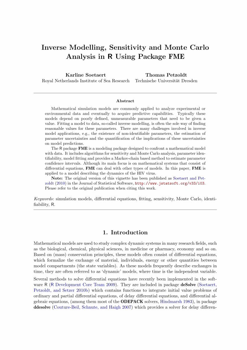
The example models the dynamics of the HIV virus in human blood cells (Figure 1)
The model describes three components, comprising the number of uninfected (T ) and infected(I) CD4+ T lymphocytes, and the number of free virions (V ). It consists of three differentialequations:

4 Inverse Modelling, Sensitivity and Monte Carlo Analysis in R Using Package FME
λ
ρ T
c V
β T V
δ I
T cells (T)
Infected (I)
Virus (V) *n
Figure 1: Schematic representation of the HIV test model.
dT
dt= λ− ρT − βTV (1)
dI
dt= βTV − δI (2)
dV
dt= nδI − cV − βTV (3)
with initial conditions (numbers at t = 0):
T (0) = T0
I(0) = I0
V (0) = V0
These equations express the rate of change of the components ( d.dt) as a sum of the sources
minus the sinks. Uninfected cells are created from sources within the body (e.g., the thymus)at rate λ, they die off at a constant rate ρ, and become infected. The latter process isproportional to the product of the number of uninfected cells and the number of virions,by a parameter (β). δ is the death rate of infected cells, and n the number of virions thatare released during lysis of one infected cell (the burst size); c is the rate at which virionsdisappear.
In practical cases, the parameters from this model are estimated based on clinical data ob-tained from individual patients. As it is more costly to measure the number of infected cells, I,(Xia 2003), this compartment is often not monitored. The occurrence of unobserved variablesis very common in mathematical models.

Karline Soetaert, Thomas Petzoldt 5
Here we assume that both the viral load and the number of healthy CD4+ T cells have beenmeasured; the CD4+ T cells at 4 days intervals, the viral load at a higher frequency.
Without measurements of I, its initial condition, I0, is not available. Therefore, it is estimatedusing equation (3) as:
I0 =V ′0 + cV0
nδ
where V ′0 is the first derivative of the number of virions, estimated at the initial time. This
can be evaluated e.g., by fitting a spline through the initial points (Wu et al. 2008) or bysimple differencing of the first observed data points.
2.1. Implementation in R
In R, this model is implemented as a function (HIV_R) that takes as input the parametervalues (pars) and the initial conditions V0, V
′0 , T0, here called V_0, dV_0 and T_0 and that
returns the model solution at selected time points.
Two versions of the model are given.
The first, HIV_R consists only of R code. The function contains the derivative function derivs,required by the integration routine (see help of deSolve). It calculates the rate of change ofthe three state variables (dT, dI, dV) and an output variable, the logarithm of the numberof virions (logV). Viral counts are often represented logarithmically (Wu et al. 2008). Afterinitialising the state variables (y), and specifying the output times (times), the model isintegrated using deSolve function ode and the output returned as a data.frame.
R> HIV_R <- function (pars, V_0 = 50000, dV_0 = -200750, T_0 = 100) {
+
+ derivs <- function(time, y, pars) {
+ with (as.list(c(pars, y)), {
+ dT <- lam - rho * T - bet * T * V
+ dI <- bet * T * V - delt * I
+ dV <- n * delt * I - c * V - bet * T * V
+
+ return(list(c(dT, dI, dV), logV = log(V)))
+ })
+ }
+
+ # initial conditions
+ I_0 <- with(as.list(pars), (dV_0 + c * V_0) / (n * delt))
+ y <- c(T = T_0, I = I_0, V = V_0)
+
+ times <- c(seq(0, 0.8, 0.1), seq(2, 60, 2))
+ out <- ode(y = y, parms = pars, times = times, func = derivs)
+
+ as.data.frame(out)
+ }
6 Inverse Modelling, Sensitivity and Monte Carlo Analysis in R Using Package FME
In the second version of the model (HIV), the derivative function has been replaced by asubroutine written in Fortran, and presented to R as a DLL (a dynamic link library FME.dll onWindows respectively a shared library FME.so on other operating systems). This DLL containstwo subroutines: derivshiv estimates the derivatives, and inithiv initialises the model.How to write model code in compiled languages is explained in vignette (“compiledCode”)(Soetaert, Petzoldt, and Setzer 2009) in package deSolve. The Fortran code required for thissecond implementation can be found in the appendix; the DLL is part of the FME package.
R> HIV <- function (pars, V_0 = 50000, dV_0 = -200750, T_0 = 100) {
+
+ I_0 <- with(as.list(pars), (dV_0 + c * V_0) / (n * delt))
+ y <- c(T = T_0, I = I_0, V = V_0)
+
+ times <- c(0, 0.1, 0.2, 0.4, 0.6, 0.8, seq(2, 60, by = 2))
+ out <- ode(y = y, parms = pars, times = times, func = "derivshiv",
+ initfunc = "inithiv", nout = 1, outnames = "logV", dllname = "FME")
+
+ as.data.frame(out)
+ }
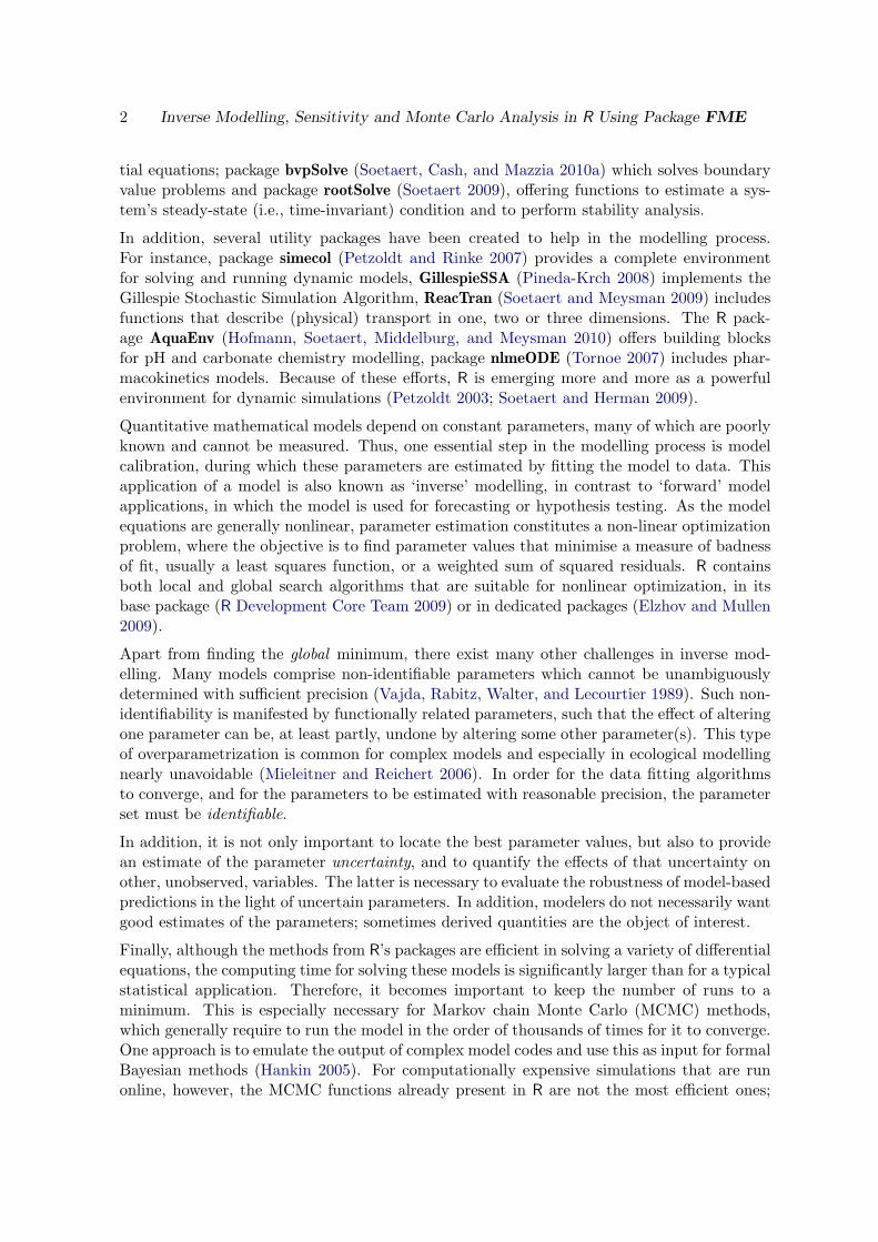
After assigning values to the parameters and running the model, output is plotted (Figure 2).It takes about 20 times longer to run the pure-R version, compared to the compiled version.As this will be significant when running the model multiple times, in what follows, the fastversion (HIV) will be used.
R> pars <- c(bet = 0.00002, rho = 0.15, delt = 0.55, c = 5.5, lam = 80, n = 900)
R> out <- HIV(pars = pars)
R> par(mfrow = c(1, 2))
R> plot(out$time, out$logV, main = "Viral load", ylab = "log(V)",
+ xlab = "time", type = "b")
R> plot(out$time, out$T, main = "CD4+ T", ylab = "-", xlab = "time", type = "b")
R> par(mfrow = c(1, 1))
2.2. Observed data
The FME algorithms will be tested on simulated data. Such synthetic experiments are oftenused to study parameter identifiability or to test fitting routines.
They involve the following steps: first “data” are generated by applying the model withknown parameter values. To this output, a normally distributed error, with mean 0 andknown standard deviation is added. Here the standard deviation is 0.45 for log (viral load)and 4.5 for the T cell counts (Xia 2003). The data are in a matrix containing the time, thevariable value and the standard deviation.
The virions have been counted at high frequency:

Karline Soetaert, Thomas Petzoldt 7
●
●
●
●
●●
●
●
●● ● ●
●●
●● ● ● ● ● ● ● ● ● ● ● ● ● ● ● ● ● ● ● ● ●
0 10 20 30 40 50 60
8.5
9.0
9.5
10.5
Viral load
time
log(
V)
●●●●●●
●
●
●
●
●●
● ● ●●
●● ● ● ● ● ● ● ● ● ● ● ● ● ● ● ● ● ● ●
0 10 20 30 40 50 60
100
150
200
250
300
CD4+ T
time−
Figure 2: Viral load and number of uninfected T cells as a function of time.
R> DataLogV <- cbind(time = out$time,
+ logV = out$logV + rnorm(sd = 0.45, n = length(out$logV)),
+ sd = 0.45)
The T cells are recorded at 4-days intervals; [ii] selects the model output that correspondsto these sampling times.
R> ii <- which (out$time %in% seq(0, 56, by = 4))
R> DataT <- cbind(time = out$time[ii],
+ T = out$T[ii] + rnorm(sd = 4.5, n = length(ii)),
+ sd = 4.5)
R> head(DataT)
time T sd
[1,] 0 97.54154 4.5
[2,] 4 206.91401 4.5
[3,] 8 292.08836 4.5
[4,] 12 336.39283 4.5
[5,] 16 332.48466 4.5
[6,] 20 320.31275 4.5
2.3. The model cost function
The model-data residuals and model cost are central to the parameter identifiability, modelcalibration and MCMC analysis.
Function modCost estimates weighted residuals of the model output versus the data andcalculates sums of squared residuals, in an object of class modCost.
8 Inverse Modelling, Sensitivity and Monte Carlo Analysis in R Using Package FME
For any observed data point, k, of observed variable l, the weighted and scaled residuals areestimated as:
resk,l =Modk,l −Obsk,lerrork,l · nl
where Modk,l and Obsk,l are the modeled, respectively observed value.
errork,l is a weighing factor that makes the term non-dimensional; it can be chosen to beequal to the mean of all measurements, the overall standard deviation, or chosen to be adifferent measurement error for each data point 1. Weighing is important if different modelvariables have different units and magnitudes.
Some variables are measured at much higher resolution than others. In order to prevent theabundant data set to dominate the analysis, the residuals can also be scaled relative to thenumber of data points nl for each variable l; by default nl is 1.
Sums of these residuals per observed variable (the“variable”cost) and the total sum of squares(the “model” cost) are also estimated in function modCost.
For the HIV model example, the residuals and costs are estimated in a function (HIVcost) thattakes as input the values of the parameters to be tested/fitted. The model cost is calculatedin three steps. First, the model output, given the current parameter values is produced (out);then the residuals with the log(V ) data, in matrix DataLogV, is estimated (cost); argumenterr = "sd" specifies the columnname with the weighting factors. Finally the cost is updatedwith the T cell observations in matrix DataT. Updating is done by passing the previouslyestimated cost (cost = cost) to function modCost.
R> HIVcost <- function (pars) {
+ out <- HIV(pars)
+ cost <- modCost(model = out, obs = DataLogV, err = "sd")
+ return(modCost(model = out, obs = DataT, err = "sd", cost = cost))
+ }
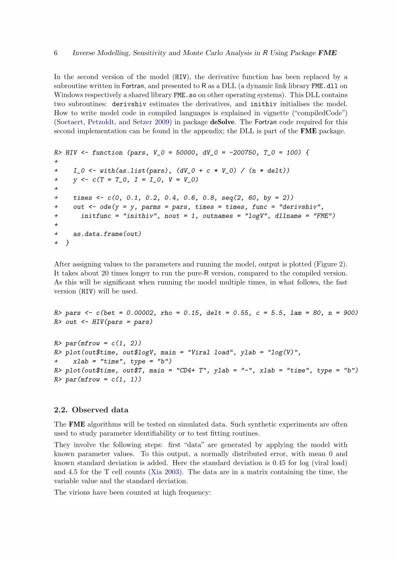
The sum of squared residuals is printed, and the residuals of model and data plotted, showingthe random noise (Figure 3).
R> HIVcost(pars)$model
[1] 47.55381
R> plot(HIVcost(pars), xlab="time")
3. Local sensitivity analysis
1modCost assumes the measurement errors to be normally distributed and independent. If there exist
correlations in the errors between the measurements, then modCost should not be used in the fitting or MCMCapplication, but rather a function that takes in to account the data covariances.

Karline Soetaert, Thomas Petzoldt 9
●
●
●
●
● ●
●
●
●
●
●
●
●
●
●
0 10 20 30 40 50 60
−3
−2
−1
01
2
time
wei
ghte
d re
sidu
als
● TlogV
Figure 3: Residuals of model and pseudodata.
Not all parameters can be finetuned on a certain data set. Some parameters have little effecton the model outcome, while other parameters are so closely related that they cannot befitted simultaneously.
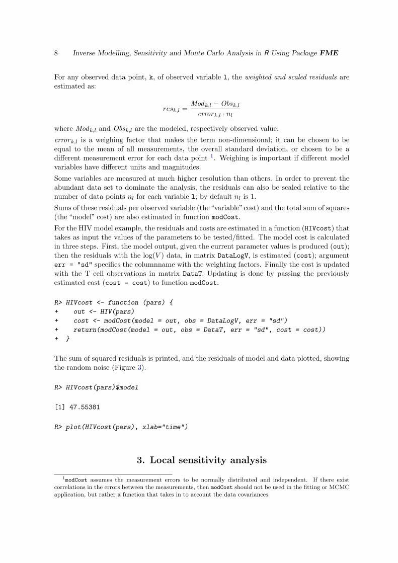
Function sensFun estimates the sensitivity of the model output to the parameter values in a setof so-called sensitivity functions (Brun et al. 2001; Soetaert and Herman 2009). When appliedin conjunction with observed data, sensFun estimates, for each datapoint, the derivative ofthe corresponding modeled value with respect to the selected parameters. A schema of whatthese sensitivity functions represent can be found in Figure 4.
In FME, normalised, dimensionless sensitivities of model output to parameters are in a sen-sitivity matrix whose (i,j)th element Si,j contains:
∂yi∂Θj
·wΘj
wyi
where yi is an output variable, Θj is a parameter, and wyi is the scaling of variable yi (usuallyequal to its value), wΘj
is the scaling of parameter Θj (usually equal to the parameter value).
These sensitivity functions can be collapsed into summary values. The higher the absolutesensitivity value, the more important the parameter, thus the magnitudes of the sensitivitysummary values can be used to rank the importance of parameters on the output variables.As it makes no sense to finetune parameters that have little effect, this ranking serves tochoose candidate parameters for model fitting.
In FME, sensitivity functions are estimated using function sensFun which takes as input thecost function (HIVcost that returns an instance of class modCost) and the parameter values.

10 Inverse Modelling, Sensitivity and Monte Carlo Analysis in R Using Package FME
0 10 20 30 40 50 60
8.5
9.0
9.5
10.0
10.5
local sensitivity, parameter bet
time
logV
bet=2e−5bet=2.2e−5
●
●
●● ●
Sensitivity functions
Figure 4: The sensitivity functions of logV to parameter bet, as a function of time (upperright) are the (weighted) differences of the perturbed output (at bet = 2.2e-5) with thenominal output (bet = 2e-5), main figure; the dots in the inset correspond to the arrows inthe main figure.

Karline Soetaert, Thomas Petzoldt 11
0 10 20 30 40 50 60
−0.
4−
0.2
0.0
0.2
0.4
logV
time
sens
itivi
ty
0 10 20 30 40 50 60
−1.
00.
00.
51.
0
T
time
sens
itivi
ty
betrhodeltclamn
Figure 5: Sensitivity functions of model output to parameters.
R> Sfun <- sensFun(HIVcost, pars)
R> summary(Sfun)
value scale L1 L2 Mean Min Max N
bet 2.0e-05 2.0e-05 0.364 0.074 -0.1594 -1.28 0.30 51
rho 1.5e-01 1.5e-01 0.117 0.020 -0.1017 -0.34 0.16 51
delt 5.5e-01 5.5e-01 0.032 0.008 0.0014 -0.11 0.21 51
c 5.5e+00 5.5e+00 0.414 0.076 0.0877 -0.43 1.32 51
lam 8.0e+01 8.0e+01 0.214 0.038 0.1863 -0.28 0.80 51
n 9.0e+02 9.0e+02 0.417 0.077 -0.0861 -1.29 0.42 51
Here L1 =∑
|Sij |/n and L2 =√
∑
(S2ij)/n are the L1 and L2 norm respectively.
Based on these summary statistics it is clear that parameter delt has the least effect on theoutput variables.
The sensitivities of the modelled viral and T cell counts to the parameter values change intime (see Figure 4), thus it makes sense to visualise the sensitivity functions as they fluctuate.The plots are clearest if produced one per output variable (Figure 5):
R> plot(Sfun, which = c("logV", "T"), xlab="time", lwd = 2)
As their corresponding sensitivity functions are always positive, parameters bet, lam, and n
have a consistent positive effect on the number of free virions; higher values of rho consistentlydecrease logV. The initial positive effect on viral load when increasing viral loss (c) is causedby its impact on the calculated initial condition I_0.
There is strong similarity in several sensitivity functions for the output variable logV, indicat-ing that the corresponding parameters have comparable effect on this output variable. If toosimilar, the joint estimation of these parameter combinations may not be possible on theseobserved data alone. The correlation between the sensitivity functions of n and lam is 1 (notshown), such that exactly the same output of logV will be generated by increasing n, if lam is

12 Inverse Modelling, Sensitivity and Monte Carlo Analysis in R Using Package FME
bet
−0.3 0.0
●●●●●●●●●●●●●●●●●●●●●●●●●●●●●●●●●●●●●
●●
●
●
● ●●
●●●●●●●
●●●●●●●●●●● ● ● ●●●●●●●●●●●●●●●●●●●●●●●
●
●●
●
●
●●●
● ●●●●●●
−0.5 0.5
●●●●●●●●●●●●●●●●●●●●●●●●●●●●●●●●●●●●
●
●●
●
●
●●●
●●●●●●●
●●●●●●●● ● ● ●●●●●●●●●●●●●●●●●●●●●●●●●●
●
●●
●
●
●●●
●●●●●●●
−1.0 0.0
−1.
00.
0
●●●●●●●●●●●●●●●●●●●●●●●●●●●●●●●●●●●●
●
●●
●
●
●●●
●●●●●●●
−0.
30.
0
−0.51 rho●●●●●●●●
●●
●●
● ●●●●●●
●●●●●●●●●●●●●●●●●
●
●
●●
●
●
●●
●●●●
●●● ●●● ●●●●●●
●●
●●●●●●
●●●●●●●●●●●●●●●●●●●
●
●
●●
●
●
●●
●●●●●●● ●●●●●●●●
●●
●●●●●●●
●●●●●●●●●●●●●●●●●●●
●
●
●●
●
●
●●
●●●●
●●● ●●●●●●●●●●●●●●●●●
●●●●●●●●●●●●●●●●●●●
●
●
●●
●
●
●●
●●●●
●●●
−0.17 −0.61 delt●●●●●●
●
●●●
●●
●●●●●●●●●●●●●●●●●●●●●●●● ●
●
●●
●
●
●●
●●●●●●● ●●●●●●
●
●● ●
●●●●●●●●●●●●●●●●●●●●●●●●●●●
●
●●
●
●
●●
●●●●●●●
−0.
100.
050.
20
●●●●●●
●
●●●
●●●●●●●●●●●●●●●●●●●●●●●●●●●
●
●●
●
●
●●
●●●●●●●
−0.
50.
5
−0.95 0.72 −0.084 c●●●●●●●
●●
●●
●●●●●●●●
●●●●●●●●●●●●●●●●●
●
●
●
●
●
●●●
●●●●●●●
●●●●●●●
●●●●●●●●●
●●●●●●●●●●●●●●●●●●●●
●
●
●
●
●
●●●
●●●●●●●
0.53 −0.94 0.52 −0.74 lam
−0.
20.
20.
6
●●●●●●●●●●●●●●●●●●●●●●●●●●●●●●●●●●●●
●
●
●
●
●
●●
●
●●●●●●●
−1.0 0.0
−1.
00.
0
1 −0.58
−0.10 0.05 0.20
−0.11 −0.97
−0.2 0.2 0.6
0.6 n
Figure 6: Pairwise plot of sensitivity functions.
decreased the appropriate amount. Similar findings were reported in Wu et al. (2008), basedon an analytical analysis of parameter identifiability.
For output variable T the similarity between parameters lam and n and bet is also strong.Pairwise relationships are visualised with a pairs plot. Here we plot the sensitivity functionsof both variables (Figure 6) in one figure but with different colors; it is also instructive to selecteach variable separately (this can be done by means of the which argument – not shown).
R> pairs(Sfun, which = c("logV", "T"), col = c("blue", "green"))
The sensitivity functions for parameter pairs involving bet, c and n, and pair rho and lam
are strongly correlated, with r2 > 0.85.
It should be noted that none of the correlation coefficients is exactly 1 or −1, (the largest|r| equals 0.995). Therefore, the model comprising both logV and T data is “algebraically”identifiable, as is indeed demonstrated by Xia (2003). However, it is questionable whetherthe subtle differences produced in the output of some parameters will be sufficient to makethem “practically” identifiable.

Karline Soetaert, Thomas Petzoldt 13
4. Multivariate parameter identifiability
The above pairs analysis investigated the identifiability of sets of two parameters. Func-tion collin extends the analysis to all possible parameter combinations, by estimating theapproximate linear dependence (“collinearity”) of parameter sets. A parameter set is said tobe identifiable, if all parameters within the set can be uniquely estimated based on (perfect)measurements. Parameters that have large collinearity will not be identifiable 2.
The identifiability analysis included in FME was described in Brun et al. (2001). For anysubset of columns of the sensitivity matrix, collinearity γ is defined as:
γ =1
√
min(EV[S⊤S])
where
Sij =Sij
√
∑
j S2ij
where S contains the columns of the sensitivity matrix that correspond to the parameters in-cluded in the set, EV estimates the eigenvalues. The collinearity index equals 1 if the columnsare orthogonal, and the set is identifiable, it equals infinity if columns in the sensitivity matrixare linearly dependent.
A collinearity index γ means that a change in the results caused by a change in one parametercan be compensated by the fraction 1−1/γ by an appropriate change of the other parameters(Omlin, Brun, and Reichert 2001).
If the index exceeds a certain value, typically chosen to be 10–15, then the parameter setis poorly identifiable (Brun et al. 2001) (any change in one parameter can be undone for 90respectively 93%).
The collinearity for all parameter combinations is estimated by function collin, taking thepreviously estimated sensitivity functions as argument.
R> ident <- collin(Sfun)
R> head(ident, n = 20)
bet rho delt c lam n N collinearity
1 1 1 0 0 0 0 2 1.1
2 1 0 1 0 0 0 2 1.1
3 1 0 0 1 0 0 2 4.2
4 1 0 0 0 1 0 2 1.1
5 1 0 0 0 0 1 2 8.1
6 0 1 1 0 0 0 2 1.4
7 0 1 0 1 0 0 2 1.3
8 0 1 0 0 1 0 2 5.4
9 0 1 0 0 0 1 2 1.2
10 0 0 1 1 0 0 2 1.0
11 0 0 1 0 1 0 2 1.3
2The reverse need not be the case, as unidentifiable parameters may also be non-linearly related.

14 Inverse Modelling, Sensitivity and Monte Carlo Analysis in R Using Package FME
2 3 4 5 6
12
510
2050
Collinearity
Number of parameters
Col
linea
rity
inde
x
Figure 7: Collinearity plot.
12 0 0 1 0 0 1 2 1.1
13 0 0 0 1 1 0 2 1.3
14 0 0 0 1 0 1 2 6.3
15 0 0 0 0 1 1 2 1.2
16 1 1 1 0 0 0 3 1.5
17 1 1 0 1 0 0 3 7.0
18 1 1 0 0 1 0 3 5.4
19 1 1 0 0 0 1 3 27.3
20 1 0 1 1 0 0 3 6.3
In the output, 1 and 0 denotes that the parameter is included respectivity not included inthe set; N is the number of parameters in the set.
The first 20 combinations show very large collinearity when parameters bet, rho and n arein the parameter set. Figure 7 shows how the collinearity index increases as more and moreparameters are included in the set.
R> plot(ident, log = "y")
All parameters together have a collinearity which is too large for them to be fitted to thedata. Thus, whereas Xia (2003) showed the full parameter set to be algebraically identifiable,in practical applications this may not be the case.
R> collin(Sfun, parset = c("bet", "rho", "delt", "c", "lam", "n"))
Karline Soetaert, Thomas Petzoldt 15
bet rho delt c lam n N collinearity
1 1 1 1 1 1 1 6 53
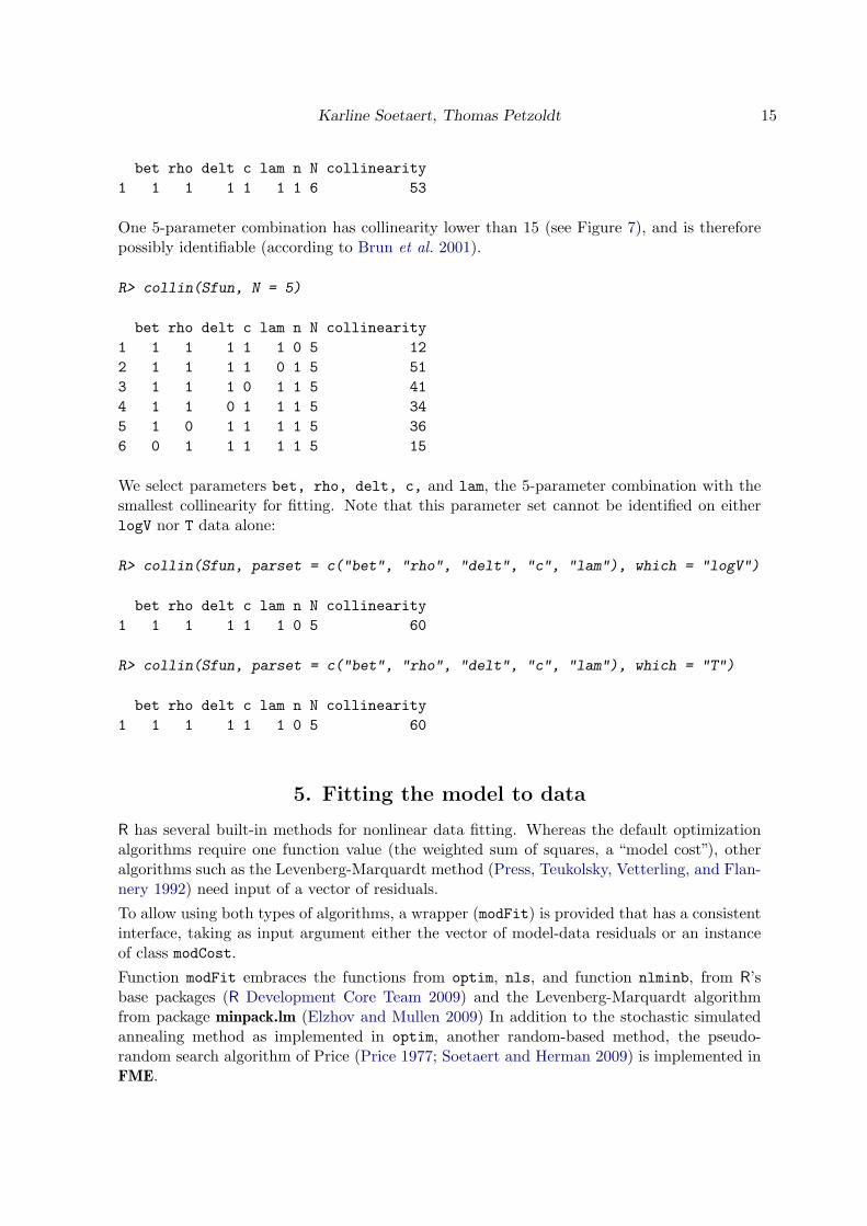
One 5-parameter combination has collinearity lower than 15 (see Figure 7), and is thereforepossibly identifiable (according to Brun et al. 2001).
R> collin(Sfun, N = 5)
bet rho delt c lam n N collinearity
1 1 1 1 1 1 0 5 12
2 1 1 1 1 0 1 5 51
3 1 1 1 0 1 1 5 41
4 1 1 0 1 1 1 5 34
5 1 0 1 1 1 1 5 36
6 0 1 1 1 1 1 5 15
We select parameters bet, rho, delt, c, and lam, the 5-parameter combination with thesmallest collinearity for fitting. Note that this parameter set cannot be identified on eitherlogV nor T data alone:
R> collin(Sfun, parset = c("bet", "rho", "delt", "c", "lam"), which = "logV")
bet rho delt c lam n N collinearity
1 1 1 1 1 1 0 5 60
R> collin(Sfun, parset = c("bet", "rho", "delt", "c", "lam"), which = "T")
bet rho delt c lam n N collinearity
1 1 1 1 1 1 0 5 60
5. Fitting the model to data
R has several built-in methods for nonlinear data fitting. Whereas the default optimizationalgorithms require one function value (the weighted sum of squares, a “model cost”), otheralgorithms such as the Levenberg-Marquardt method (Press, Teukolsky, Vetterling, and Flan-nery 1992) need input of a vector of residuals.
To allow using both types of algorithms, a wrapper (modFit) is provided that has a consistentinterface, taking as input argument either the vector of model-data residuals or an instanceof class modCost.
Function modFit embraces the functions from optim, nls, and function nlminb, from R’sbase packages (R Development Core Team 2009) and the Levenberg-Marquardt algorithmfrom package minpack.lm (Elzhov and Mullen 2009) In addition to the stochastic simulatedannealing method as implemented in optim, another random-based method, the pseudo-random search algorithm of Price (Price 1977; Soetaert and Herman 2009) is implemented inFME.

16 Inverse Modelling, Sensitivity and Monte Carlo Analysis in R Using Package FME
To fit the HIV model to the data, a new function is needed that takes as input the logarithmof all parameter values except n (which is given a fixed value 900), and that returns the modelcost.
The log transformation (1) ensures that the parameters remain positive during the fitting, and(2) deals with the fact that the parameter values are spread over six orders of magnitude (i.e.,bet = 2e-5, lam = 80). Within the function HIVcost2, the parameters are backtransformed(exp(lpars)).
R> HIVcost2 <- function(lpars)
+ HIVcost(c(exp(lpars), n = 900))
After perturbing the parameters3, the model is fitted to the data, and best-fit parameters andresidual sum of squares shown.
R> Pars <- pars[1:5] * 2
R> Fit <- modFit(f = HIVcost2, p = log(Pars))
R> exp(coef(Fit))
bet rho delt c lam
2.133068e-05 1.433727e-01 5.876967e-01 5.870447e+00 8.093473e+01
R> deviance(Fit)
[1] 44.62702
For comparison, the initial model output and the best-fit model are plotted against the data(Figure 8).
R> ini <- HIV(pars = c(Pars, n = 900))
R> final <- HIV(pars = c(exp(coef(Fit)), n = 900))
R> par(mfrow = c(1,2))
R> plot(DataLogV, xlab = "time", ylab = "logV", ylim = c(7, 11))
R> lines(ini$time, ini$logV, lty = 2)
R> lines(final$time, final$logV)
R> legend("topright", c("data", "initial", "fitted"),
+ lty = c(NA,2,1), pch = c(1, NA, NA))
R> plot(DataT, xlab = "time", ylab = "T")
R> lines(ini$time, ini$T, lty = 2)
R> lines(final$time, final$T)
R> par(mfrow = c(1, 1))
Approximate estimates of parameter uncertainty can be obtained by linearising the modelaround the best-fit parameters. If J is the numerical approximation of the Jacobian, then,
3Perturbation is done mainly for the purpose of making the application more challenging.

Karline Soetaert, Thomas Petzoldt 17
●
●
●
●
●
●●
●
●
●
●
●
●
●
●●
●●
●
●
●
● ●●
●
●
●●
●
● ●●
● ●
●
●
0 10 20 30 40 50 60
78
910
11
time
logV
● datainitialfitted
●
●
●
● ●●
● ● ● ● ●● ● ●
●
0 10 20 30 40 50
100
150
200
250
300
timeT
Figure 8: Best-fit and initial model run.
based on linear theory, the parameter covariance is estimated as (J⊤J)−1S2 where S2 is thesum of squared residuals of the best-fit. At the best fit, (J⊤J) ≈ 0.5H, with H the Hessian(Press et al. 1992). The Hessian is estimated in most of R’s optimization functions.
The summarymethod of the modFit function estimates these approximate statistical properties(not shown).
6. MCMC
The previously applied identifiability analysis (Section 4) gives insight into which parameterscan be simultaneously estimated, given noise-free data and a perfect model (i.e., one that canfit the data perfectly). The model fitting (Section 5) provided one“optimal” set of parameters,that produces the best fit to the measurements in the least squares sense.
However, even for perfectly identifiable parameter sets, the uncertainty may be very highor poor estimates may be obtained, if the data have too much noise. In practice, all mea-surements have error, thus it is important to quantify the effect of this on the parameteruncertainty.
Bayesian methods can be used to derive the data-dependent probability distribution of theparameters. Function modMCMC implements a Markov chain Monte Carlo (MCMC) methodthat uses the delayed rejection and adaptive Metropolis (DRAM) procedure (Haario et al.2006; Laine 2008). An MCMC method samples from probability distributions by constructinga Markov chain that has the desired distribution as its equilibrium distribution. Thus, ratherthan one parameter set, one obtains an ensemble of parameter values that represent theparameter distribution.
In the adaptive Metropolis method, the generation of new candidate parameter values ismade more efficient by tuning the proposal distribution to the size and shape of the targetdistribution. This is realised by generating new parameters with a proposal covariance matrix

18 Inverse Modelling, Sensitivity and Monte Carlo Analysis in R Using Package FME
that is estimated by the parameters generated thus far.
During delayed rejection, new parameter values are tried upon rejection by scaling the pro-posal covariance matrix. This provides a systematic remedy when the adaptation process hasa slow start (Haario et al. 2006).
In the implementation in FME, it is assumed that the prior distribution for the parameters θis either non-informative or gaussian.
If y, the measurements are defined as:
y = f(x, θ) + ξ
ξ ∼ N(
0, σ2)
where f(x, θ) is the (nonlinear) model, x are the independent variables, θ the parameters, andξ is the additive, independent Gaussian error, with unknown variance σ2. Then the posteriorfor the parameters will be estimated as (Laine 2008):
p(
θ|y, σ2)
∝ exp
(
−0.5 ·
(
SS(θ)
σ2
))
· ppri(θ)
where SS is the sum of squares function SS(θ) =∑
(yi − f(x, θ)i)2, ppri(θ) is the prior
distribution of the parameters. For noninformative priors ppri(θ) is constant for all values ofθ (and can be ignored).
The error variance σ2 is considered a nuisance parameter (Gelman, Varlin, Stern, and Rubin2004). A prior distribution needs to be specified and a posterior distribution is calculated bymodMCMC. For the reciprocal of the error variance (σ−2), a Gamma distribution is used as aprior:
ppri(
σ−2)
∼ Γ(n0
2,n0
2S20
)
At each MCMC step then, the reciprocal of the error variance is sampled from a gammadistribution (Gelman et al. 2004):
p(
σ−2|(y, θ))
∼ Γ
(
n0 + n
2,n0S
20 + SS(θ)
2
)
In function modMCMC, the corresponding input arguments for this Gamma distribution are var0= S2
0 and n0 = wvar0 * n, and where wvar0 or n0 are input arguments to the function; n isthe number of observations. Larger values of wvar0 keep the sampled error variance closer tovar0.
The MCMC method is now applied to the example model. In order to prevent long burn-in,the algorithm is started with the optimal parameter set (Fit$par) as returned from the fittingalgorithm, while the prior error variance var0 is chosen to be the mean of the unweightedsquared residuals from the model fit (Fit$var_ms_unweighted); one for each observed vari-able (i.e., one for logV, one for T). The weight added to this prior is low (wvar0 = 0.1), suchthat this initial value is not so important.
The proposal distribution (used to generate new parameters) is updated every 50 iterations(updatecov). The initial proposal covariance (jump) is based on the approximated covariance
Karline Soetaert, Thomas Petzoldt 19
matrix, as returned by the summary method of modFit, and scaled appropriately (Gelmanet al. 2004).
R> var0 <- Fit$var_ms_unweighted
R> cov0 <- summary(Fit)$cov.scaled * 2.4^2/5
R> MCMC <- modMCMC(f = HIVcost2, p = Fit$par, niter = 5000, jump = cov0,
+ var0 = var0, wvar0 = 0.1, updatecov = 50)
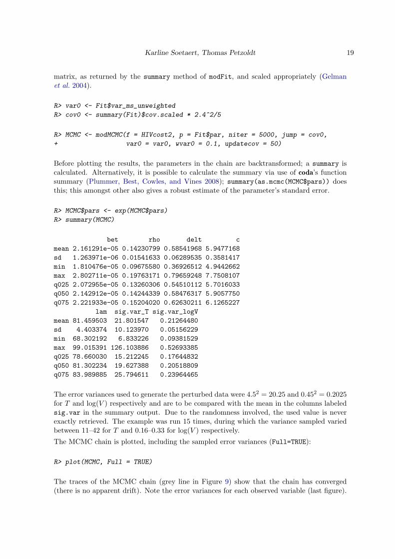
Before plotting the results, the parameters in the chain are backtransformed; a summary iscalculated. Alternatively, it is possible to calculate the summary via use of coda’s functionsummary (Plummer, Best, Cowles, and Vines 2008); summary(as.mcmc(MCMC$pars)) doesthis; this amongst other also gives a robust estimate of the parameter’s standard error.
R> MCMC$pars <- exp(MCMC$pars)
R> summary(MCMC)
bet rho delt c
mean 2.161291e-05 0.14230799 0.58541968 5.9477168
sd 1.263971e-06 0.01541633 0.06289535 0.3581417
min 1.810476e-05 0.09675580 0.36926512 4.9442662
max 2.802711e-05 0.19763171 0.79659248 7.7508107
q025 2.072955e-05 0.13260306 0.54510112 5.7016033
q050 2.142912e-05 0.14244339 0.58476317 5.9057750
q075 2.221933e-05 0.15204020 0.62630211 6.1265227
lam sig.var_T sig.var_logV
mean 81.459503 21.801547 0.21264480
sd 4.403374 10.123970 0.05156229
min 68.302192 6.833226 0.09381529
max 99.015391 126.103886 0.52693385
q025 78.660030 15.212245 0.17644832
q050 81.302234 19.627388 0.20518809
q075 83.989885 25.794611 0.23964465
The error variances used to generate the perturbed data were 4.52 = 20.25 and 0.452 = 0.2025for T and log(V ) respectively and are to be compared with the mean in the columns labeledsig.var in the summary output. Due to the randomness involved, the used value is neverexactly retrieved. The example was run 15 times, during which the variance sampled variedbetween 11–42 for T and 0.16–0.33 for log(V ) respectively.
The MCMC chain is plotted, including the sampled error variances (Full=TRUE):
R> plot(MCMC, Full = TRUE)
The traces of the MCMC chain (grey line in Figure 9) show that the chain has converged(there is no apparent drift). Note the error variances for each observed variable (last figure).

20 Inverse Modelling, Sensitivity and Monte Carlo Analysis in R Using Package FME
0 2000 40001.8e
−05
2.6e
−05
bet
iter
0 2000 4000
0.10
0.14
0.18
rho
iter
0 2000 4000
0.4
0.6
0.8
delt
iter
0 2000 4000
5.0
6.0
7.0
c
iter
0 2000 4000
7080
9010
0
lam
iter
0 2000 4000
200
500
800
SSR
iter
0 2000 4000
1050
var_T
iter
varia
nce
0 2000 4000
0.1
0.2
0.4
var_logV
iter
varia
nce
Figure 9: Results of the MCMC application.
Karline Soetaert, Thomas Petzoldt 21
bet
0.10 0.14 0.18
●
●●●
●
●
●
●●
●●
●
●
●●
●●
●●
●
●
●●
●
●
●
●
●●
●●
●
●●
●
●●
●
●
●●●
●
●
● ●
●● ●
●
●
●●
●
●●
●
●
●
●
●
●
●
●
●
●
●●
●
●
● ●
●
●
●
●●
●
●
●
●
●
●
●
●●●
●
●
●
●
●●
●
●
●●●
●
●
●
●
●
●
● ●
●
●
●
●
●
●
●
●
●
●
●
●
●
●●●
●
●●
●
●● ●
●
●●
●
●
● ● ●
●
●
●
●●
●●
●●
●
●●
●
●
●●
●
●
●
●
●● ●
●
● ●
●
●
●
●●
●●
●
●
●
●
●
●
●
●
●●●
●
●
●●
●
●
●●
●●
●
●●
●
●
●●●
●
●
●
●
● ●
●
●●
●●
●
●●
●
●
●●
●
●
●
●
●● ●
●
●
●
●
●●
●
●
●
●
●
●
●
●●
●
●
●●
●
●
●
●
●
●
●●●
●
●●
●● ●●
●
●●
●
●
●●
●
●●
●
● ●● ●
●●
●
●●●
●
●
●
●
●
●
●
●●
●
●
●
● ●●
●●
●
●
●
● ●
●
●
●●
●
●
●
●
●
●●●●●
●●●
●
●
●●●
●
● ●●
●
●● ●●
●
●
●
●●
●●●
●
●
●
●●
●
●
●
●
●
●
●
●
●
●
●
●●
●
●
●
● ● ●●
●
●
●
●
●●●●
●●
●
●●
●
●●
●●
●
●
●
●●● ●●
●
●● ●
●
●
●
●●
●
●
●
●
●●●●
●
●● ●
●●
● ●●
●
●●
● ●
●
●
●●
●●
● ●
●
●
●
●●●●
●
●
●
●●
●●
●
●●
●●
●
●●●
●
●
●
●
●●●
●●
●
●
●
●
●
●
●●
●●●
●
●
●●
●
●●
●
●
●
●
●
●
● ●●
●●
●●
●
●●
●
●
●●
●●
●
●●
●
●
●
●
●
●
●●●
●
●●
●●
●●●
●
●
●
●●
●
●
●
●
●
●
●
●
●
●
●
●
●●
●●●
●
●●
●
●●
●●
●
●
●
●
●●
●●
●
●
●●● ●
●
●●●
●●
●
●
●
●●
●
●
●●
● ●●
●
●
●
●
●
●
●
●
●●●
●
●
●
●
●
●
●●●
●●
●●
●
●
● ●
●●
●
●
●
●
●●
●●
●
●
●
●●
●
●
●
●
●
●
●
●
●
●
●●
●● ●
●● ●
●
●
●
●
●●
●
●
●
●●
●
●●●
●
●
●
●
●
●
● ●
●
●
●
●
●●
●●
●
●
●●
●
●● ●
●●
●●
●
●
●
●
●
● ●
●
●
●
●●
●
●
●
●●
●
●
●
●
●
●
●
●●
●
●
●
●● ●
●
● ●
●
●
●
●
●
●
●
●
●
●
●
●
●●
●
●
●
●●
●
●●
●
●
●
●
●
●
●
●
●
● ●
●●
●
●
● ●●
●
●
●
●
●
●●
●●●
●
●
● ●●
●
●●
●●
●
● ●
●
●●
●
●●
●●●●
●●
●●
●●
●●
●
●
●
●
●
●
● ●
●
●
●
●
●
●
● ●● ●● ●
●
●● ●
●
●
●
●●
●●
●● ●
●
●
●
●
●
●
●
●
●
●● ●●
●●
●● ●● ●●●
●●●
●
●
●
●●
●
●
●●
●
●
●
●
●●
●
●
●
●●●
●
●●
●
●
●
●
●●
●
●
●
●●
●●
●●
●
●
●●
●
● ●●
●
●●●
●● ●
●
●
●
●●
● ●
●●●●
●●
●
●
●
●
●● ●
●●
●
●
●
●
●●
●●
●
●
●
●
●
●
● ●
●
●●
●●
●●
●
●
● ●
●
●● ●
●●
●
●
●
●
●●
●
●
●
●
●●
●
●
●●
●
●
●
●
●
●
●
●●
●●
●
●●●
●
●
●
●●
●●
●
●
●●
●●
●●
●
●
●●
●
●
●
●
●●
●●
●
●●
●
●●
●
●
●●●
●
●
● ●
●●●
●
●
●●
●
●●
●
●
●
●
●
●
●
●
●
●
●●
●
●
●●
●
●
●
●●
●
●
●
●
●
●
●
●●●
●
●
●
●
●●
●
●
●●●
●
●
●
●
●
●
● ●
●
●
●
●
●
●
●
●
●
●
●
●
●
●●●
●
●●
●
●● ●
●
●●
●
●
● ● ●
●
●
●
●●
● ●
●●
●
●●
●
●
●●
●
●
●
●
●● ●
●
● ●
●
●
●
●●
●●
●
●
●
●
●
●
●
●
● ●●
●
●
●●
●
●
●●
●●
●
●●
●
●
●●●
●
●
●
●
● ●
●
●●
●●
●
●●
●
●
●●
●
●
●
●
●●●
●
●
●
●
●●
●
●
●
●
●
●
●
●●
●
●
●●
●
●
●
●
●
●
●●●
●
●●
●●●●
●
●●
●
●
●●
●
●●
●
● ●● ●
●●
●
● ● ●
●
●
●
●
●
●
●
●●
●
●
●
● ●●
●●
●
●
●
●●
●
●
●●
●
●
●
●
●
●●●●●
●● ●
●
●
●●●
●
● ●●
●
●● ●●
●
●
●
●●
●●
●●
●
●
●●
●
●
●
●
●
●
●
●
●
●
●
●●
●
●
●
● ●●●
●
●
●
●
●●●●
●●
●
●●
●
●●
●●
●
●
●
●●● ●●
●
●● ●
●
●
●
●●
●
●
●
●
● ●●●
●
●● ●
●●
● ●●
●
●●
●●
●
●
●●
●●
● ●
●
●
●
●●● ●
●
●
●
●●
●●
●
●●
●●
●
●●●
●
●
●
●
●●
●
●●
●
●
●
●
●
●
●●
●● ●
●
●
●●
●
●●
●
●
●
●
●
●
● ●●
●●
●●
●
●●
●
●
●●● ●
●
●●
●
●
●
●
●
●
●●●
●
●●
●●
●●●
●
●
●
●●
●
●
●
●
●
●
●
●
●
●
●
●
●●
●●
●
●
●●
●
●●
●●
●
●
●
●
●●
●●
●
●
●●● ●
●
●●●●
●●
●
●
●●
●
●
●●
● ●●
●
●
●
●
●
●
●
●
●●●
●
●
●
●
●
●
●●●
● ●
●●
●
●
● ●
●●
●
●
●
●
●●
●●
●
●
●
●●
●
●
●
●
●
●
●
●
●
●
● ●
●● ●
●●●
●
●
●
●
●●
●
●
●
●●
●
●●
●●
●
●
●
●
●
● ●
●
●
●
●
●●
●●
●
●
●●
●
●● ●
●●
●●
●
●
●
●
●
● ●
●
●
●
●●
●
●
●
●●
●
●
●
●
●
●
●
● ●
●
●
●
●● ●
●
● ●
●
●
●
●
●
●
●
●
●
●
●
●
●●
●
●
●
●●
●
●●
●
●
●
●
●
●
●
●
●
● ●
●●
●
●
●●●
●
●
●
●
●
●●
● ●●
●
●
● ●●
●
●●
●●
●
● ●
●
●●
●
●●
●●●●
●●
●●
●●
●●
●
●
●
●
●
●
●●
●
●
●
●
●
●
● ●● ●● ●
●
●● ●
●
●
●
●●
●●
●● ●
●
●
●
●
●
●
●
●
●
●● ●●
●●
●●●● ●●●
●●●
●
●
●
●●
●
●
●●
●
●
●
●
●●
●
●
●
●●●
●
● ●
●
●
●
●
●●
●
●
●
●●
●●
●●
●
●
●●
●
● ●●
●
●●●
●● ●
●
●
●
●●
● ●
●●●●
●●
●
●
●
●
●● ●
●●
●
●
●
●
●●
●●
●
●
●
●
●
●
●●
●
●●
●●
●●
●
●
● ●
●
●●●
●●
●
●
●
●
●●
●
●
●
●
●●
●
●
●●
●
●
●
●
●
●
●
●●
●●
5.0 6.0 7.0
●
●●
●
●
●
●
●●
●●
●
●
●●
●●
●●
●
●
●●
●
●
●
●
●●
●●
●
●●
●
●●
●
●
●●●
●
●
●●
●●●
●
●
●●
●
●●
●
●
●
●
●
●
●
●
●
●
●●●
●
●●
●
●
●
●●
●
●
●
●
●
●
●
●●●
●
●
●
●
●●
●
●
●●●
●
●
●
●
●
●
●●
●
●
●
●
●
●
●
●
●
●
●
●
●
●●●
●
●●
●
●●●
●
●●
●
●
●●●
●
●
●
●●
●●
●●
●
●●
●
●
●●
●
●
●
●
●●●
●
● ●
●
●
●
●●
●●
●
●
●
●
●
●
●
●
●●●
●
●
●●
●
●
●●
●●
●
●●
●
●
●●●
●
●
●
●
●●
●
●●
●●
●
●●
●
●
●●
●
●
●
●
●●●
●
●
●
●
●●
●
●
●
●
●
●
●
●●
●
●
●●
●
●
●
●
●
●
●●●
●
●●
●●●●
●
●●
●
●
●●
●
●●
●
●●●●
●●
●
●●●
●
●
●
●
●
●
●
●●
●
●
●
●●●
●●
●
●
●
●●
●
●
●●
●
●
●
●
●
●●●●●
●●●
●
●
●●●
●
●●●
●
●●●●
●
●
●
●●
●●
●●
●
●
●●
●
●
●
●
●
●
●
●
●
●
●
●●
●
●
●
●●●●
●
●
●
●
●●●●
●●
●
●●
●
●●
●●
●
●
●
●●●●●
●
●●●
●
●
●
●●
●
●
●
●
●●●●
●
●●●
●●
●●●
●
●●
●●
●
●
●●
●●
● ●
●
●
●
●●●●
●
●
●
●●
●●
●
●●
●●
●
●●●
●
●
●
●
●●
●
●●
●
●
●
●
●
●
●●
●●●
●
●
●●
●
●●
●
●
●
●
●
●
●●●
●●
●●
●
●●
●
●
●●
●●
●
●●
●
●
●
●
●
●
●●●
●
●●
●●
●●●
●
●
●
●●
●
●
●
●
●
●
●
●
●
●
●
●
●●
●●
●
●
●●
●
●●
●●
●
●
●
●
●●
●●
●
●
●●●●
●
●●●●
●●
●
●
●●
●
●
●●
●●●
●
●
●
●
●
●
●
●
●●●
●
●
●
●
●
●
●●●
●●
●●
●
●
●●
●●
●
●
●
●
●●
●●
●
●
●
●●
●
●
●
●
●
●
●
●
●
●
●●
●●●
●●●
●
●
●
●
●●
●
●
●
●●
●
●●
●●
●
●
●
●
●
●●
●
●
●
●
●●
●●
●
●
●●
●
●●●
●●
●●
●
●
●
●
●
●●
●
●
●
●●
●
●
●
●●
●
●
●
●
●
●
●
●●
●
●
●
●●●●
●●
●
●
●
●
●
●
●
●
●
●
●
●
●●
●
●
●
●●
●
●●
●
●
●
●
●
●
●
●
●
●●
●●
●
●
●●●
●
●
●
●
●
●●
●●●
●
●
●●●
●
●●
●●
●
●●
●
●●
●
●●
●●●●
●●
●●
●●
●●
●
●
●
●
●
●
●●
●
●
●
●
●
●
●●●●●●
●
●●●
●
●
●
●●
●●
●●●
●
●
●
●
●
●
●
●
●
●●●
●
●●
●●●●●●●
●●●
●
●
●
●●
●
●
●●
●
●
●
●
●●
●
●
●
●●●
●
●●
●
●
●
●
●●
●
●
●
●●
●●
●●
●
●
●●
●
●●●
●
●●●
●●●
●
●
●
●●
●●
●●●●
●●
●
●
●
●
●●●
●●
●
●
●
●
●●
●●
●
●
●
●
●
●
●●
●
●●
●●
●●
●
●
●●
●
●●●
●●
●
●
●
●
●●
●
●
●
●
●●
●
●
●●
●
●
●
●
●
●
●
●●
●●
1.8e
−05
2.4e
−05
●
●●
●
●
●
●
●●
●●
●
●
●●
●●
●●
●
●
●●
●
●
●
●
●●
●●
●
●●
●
●●
●
●
●●●
●
●
● ●
●● ●
●
●
●●
●
●●
●
●
●
●
●
●
●
●
●
●
●●
●
●
● ●
●
●
●
●●
●
●
●
●
●
●
●
●●●
●
●
●
●
●●
●
●
●●●
●
●
●
●
●
●
● ●
●
●
●
●
●
●
●
●
●
●
●
●
●
●●●
●
●●
●
●●●
●
●●●
●
●● ●
●
●
●
●●
●●
●●
●
● ●
●
●
●●
●
●
●
●
●● ●
●
● ●
●
●
●
●●
●●
●
●
●
●
●
●
●
●
●●●
●
●
● ●
●
●
●●
●●
●
●●
●
●
● ●●
●
●
●
●
●●
●
●●
●●
●
●●
●
●
●●
●
●
●
●
●● ●
●
●
●
●
●●
●
●
●
●
●
●
●
●●
●
●
●●
●
●
●
●
●
●
●●●
●
●●
●●● ●
●
●●
●
●
●●
●
●●
●
●●● ●
●●
●
●●●
●
●
●
●
●
●
●
●●
●
●
●
● ●●
●●
●
●
●
●●
●
●
●●
●
●
●
●
●
●●●●●
●●●
●
●
●●●
●
●●●
●
●● ●●
●
●
●
●●
●●
●●
●
●
●●
●
●
●
●
●
●
●
●
●
●
●
●●
●
●
●
●● ●●
●
●
●
●
●●●●
●●
●
●●
●
●●
●●
●
●
●
●●● ●●
●
●● ●
●
●
●
● ●
●
●
●
●
●●●●
●
●●●
●●
● ●●
●
●●
● ●
●
●
●●
●●
● ●
●
●
●
●●●●
●
●
●
●●
●●
●
●●
●●
●
●●●
●
●
●
●
●●●
●●
●
●
●
●
●
●
●●
●●●
●
●
●●
●
● ●
●
●
●
●
●
●
●● ●
●●
●●
●
● ●
●
●
●●
●●
●
●●
●
●
●
●
●
●
●●●
●
●●
● ●
● ●●
●
●
●
●●
●
●
●
●
●
●
●
●
●
●
●
●
●●
●●
●
●
●●
●
●●
●●
●
●
●
●
●●
●●
●
●
●● ● ●
●
●●●●
●●
●
●
●●
●
●
●●
●●●
●
●
●
●
●
●
●
●
● ●●
●
●
●
●
●
●
●●●
●●
●●
●
●
● ●
●●
●
●
●
●
●●
●●
●
●
●
●●
●
●
●
●
●
●
●
●
●
●
●●
●● ●
●● ●
●
●
●
●
●●
●
●
●
●●
●
●●
●●
●
●
●
●
●
●●
●
●
●
●
●●
●●
●
●
●●
●
●●●
●●
●●
●
●
●
●
●
● ●
●
●
●
●●
●
●
●
●●
●
●
●
●
●
●
●
●●
●
●
●
●●●
●
●●
●
●
●
●
●
●
●
●
●
●
●
●
●●
●
●
●
●●
●
●●
●
●
●
●
●
●
●
●
●
● ●
●●
●
●
● ●●
●
●
●
●
●
●●
●● ●
●
●
● ●●
●
●●
●●
●
● ●
●
●●
●
●●
● ● ●●
●●
●●
●●
●●
●
●
●
●
●
●
●●
●
●
●
●
●
●
● ●● ●● ●
●
●● ●
●
●
●
●●●
●
●● ●
●
●
●
●
●
●
●
●
●
● ● ●●
●●
●● ●●●●●
●●●
●
●
●
●●
●
●
●●●
●
●
●
●●
●
●
●
●●●
●
●●
●
●
●
●
●●
●
●
●
●●
●●
●●
●
●
●●
●
● ●●
●
●●●
●● ●
●
●
●
●●
● ●
● ●●●
●●
●
●
●
●
●● ●
●●
●
●
●
●
●●
●●
●
●
●
●
●
●
● ●
●
●●
●●
●●
●
●
●●
●
●● ●
●●
●
●
●
●
●●
●
●
●
●
●●
●
●
●●
●
●
●
●
●
●
●
●●
●●
0.10
0.14
0.18
0.33
rho●
●
●●
●
●
●●
●●
●
●
●
●
● ●
●
●
●
●● ●
●
●
●
●
●●
●●
●
●
●
●●
●
●
●●
●●
●
●●
●●
●●
●
●● ●
● ●
●
●
●
●
●
●
●●
●
●
● ● ●●
●●
●
●
●
●
● ●
●
●
●
●
●
●
●
●
●
●
●● ●
●
●
●
●●
●
●
●
●
●
●●
●
●
●
●
●
●
●
●
●
●
●
●
●
●
●
● ●●
●
●
●
●
●●●
● ●●
●
●●●
●
●●
●●
●
●
●
●●
●
●
●
●●
●
●
●●● ●●
●
●
●
●
●
●
●
●
●
●
● ●●
●
●
●
●
●
●
●
●●
●
●
●
●●
●●●●●
●
●
●
●
●●
●
●
●
●●
●
●
●
●
●
●
●●
●●
●
●
●
●
● ●
●
●●
●●●
●●
●
●
●
●
●
●●●
●
●
●●
●
●
●
●
●
●●
●●●
●●
●
●
●
●
●
●
●
●
●●
●●
●
●
●
●
●
●
●
●
●●
●●
●●
●
●
●
●
●●
●●
●
●
●
●
●
●●
●
● ●●
●●
●
●
●
●
●
●
●
●●
●
●
●
●
● ●
●
●
●
●
●
●
●
●●
●●
●
●
●
● ●
●
●
●
●
●●
●
●
●
●
●
●
●●
●
●●
●
●
●
●
●●
●
●
●
●
●
●
●
●
●●
●
●
●
●
●
●
●
●
●
●
●●
●
●
●●
●
●
●●
●
●
●
●
●
●
●
●
●
●
●
●
●
●
● ●
●
●
●
●●
●
●●
●
●
●
●
●
●
●
●
●
●
●
●
●
●
●
●●
●
●●●
●
●●
●
●
●
●
●
●●
●
●●
●
●
●
● ●●
●●
●
●
●
●
●●
●
●
●
●
●● ●●
●
●●
●●
●
●
●
●
●●●
●
●●
●●
●●
●
●
●
●
●
●
●
●
●
●●
●
●●
●
●
●
●
●
●
●
●
●●●
●●
●
●
●
●
●●
●
●●
●
●
●●●
●
●
●
●●
●
●
●
●●●
●
●
●
●
●
●
●
●
●
●
●
●●
●
●
● ●
●
●●
●
●
●
●
●
●●
● ●
●
●●
●
●
● ●●
●
●
●
●
●
●
●
●
●
●
●
● ●●●
●
●
●
●
●
●
●●●
● ●
●
●
●
●
●
●
● ●
●
●
●●
●
●
● ●
●
●
● ●
●
●
●
●
●
●●
●
●
●
●●
●
●
●
●
●
●
●
●
● ●
●●●
●●
●●
●
●
●
●
●●
● ●●
●
●
●● ●
●
●
●
●
●
● ●
●
●
●
●
●
●
●
● ●
●
●●
●
●●
●
●
●
●
●
●
●
●
●
●
●
●
●
●
●●
●●
●
●
●
●●
●
●
●
●
●●
●●
●●
●
●●
●
●
●●●
●
●
●
●
●
●
●
●
●
●
●●
●
●
●
●
●
●●
●
●
●
●
●
●●
●
●●
●●
●
●
●
●
●●
●
●
●
●
●
●
●
●
●●
●
●●
●
●●
●● ●●
●
●
●
●
●●
●●
●
●
●
●
●
●
●
●
●●
●
●●
●
●
●
●●
●
●
●
●
●
●
●
●
●
●
●
●●
●
●●
●
●
●
●
●
●
●
●
●
●
●
●
●
●
●
●
●●
●●
●
●
●
●
●
●●
●
●
●
●
●
●
●
●
●
●
●
●
●
●
●
●
●●
●
●●●
●
●
●
●
●
●
●
●●
●
●
●
●
●
●
●
●●
●
●
●
●●
●●
●
●
●
●
●
●
●●●
●
●●●
●
●
●
●
●
●
●
●
● ●
●
●
●●
●
●
●
● ●
●
●
●●
●●
●
●
●
● ●
●●
●●
●
●
●
●
●
●
●
●●
●●
●
●●
●
●●
●
●
●●
●
● ●●
●
● ●
●
●●
●
●●
●
●●
●
●●
●
●
●
●●
●
●
●
●
●
●
●
●
●●
●
●
●
●
●
●
●
●
●
●
● ●
●
●
●●
●●
●
●
●
●
● ●
●
●
●
●● ●
●
●
●
●
●●
●●
●
●
●
●●
●
●
●●
●●
●
●●
●●
●●
●
●● ●
● ●
●
●
●
●
●
●
●●
●
●
● ● ●●
● ●
●
●
●
●
● ●
●
●
●
●
●
●
●
●
●
●
●● ●
●
●
●
●●
●
●
●
●
●
●●
●
●
●
●
●
●
●
●
●
●
●
●
●
●
●
● ●●
●
●
●
●
●●●
●●●
●
●●●
●
●●
● ●
●
●
●
●●●
●
●
●●
●
●
●● ● ●●
●
●
●
●
●
●
●
●
●
●
●●●
●
●
●
●
●
●
●
●●
●
●
●
●●
●●● ●●
●
●
●
●
●●
●
●
●
●●
●
●
●
●
●
●
●●
●●
●
●
●
●
● ●
●
●●
●●●
●●
●
●
●
●
●
●●●
●
●
●●
●
●
●
●
●
●●
●●●●
●●
●
●
●
●
●
●
●
●●
●●●
●
●
●
●
●
●
●
●●
●●
●●
●
●
●
●
●●
●●
●
●
●
●
●
●●
●
●● ●
●●
●
●
●
●
●
●
●
●●
●
●
●
●
●●
●
●
●
●
●
●
●
●●
●●
●
●
●
●●
●
●
●
●
●●
●
●
●
●
●
●
●●
●
●●
●
●
●
●
●●
●
●
●
●
●
●
●
●
●●
●
●
●
●
●
●
●
●
●
●
● ●
●
●
●●
●
●
●●
●
●
●
●
●
●
●
●
●
●
●
●
●
●
● ●
●
●
●
●●
●
●●
●
●
●
●
●
●
●
●
●
●
●
●
●
●
●
●●
●
●●●
●
●●
●
●
●
●
●
●●
●
●●
●
●
●
● ●●
●●
●
●
●
●
●●
●
●
●
●
●● ●●
●
●●
●●
●
●
●
●
●●●
●
●●
●●
●●
●
●
●
●
●
●
●
●
●
●●
●
●●
●
●
●
●
●
●
●
●
● ●●
●●
●
●
●
●
●●
●
●●
●
●
●●
●
●
●
●
●●
●
●
●
●●
●
●
●
●
●
●
●
●
●
●
●
●
●●
●
●
●●
●
●●
●
●
●
●
●
●●
●●
●
●●
●
●
● ●●
●
●
●
●
●
●
●
●
●
●
●
● ●●●
●
●
●
●
●
●
●●●
● ●
●
●
●
●
●
●
● ●
●
●
●●
●
●
●●
●
●
● ●
●
●
●
●
●
●●
●
●
●
●●
●
●
●
●
●
●
●
●
● ●
●● ●
● ●
●●
●
●
●
●
●●
● ● ●
●
●
●● ●
●
●
●
●
●
●●
●
●
●
●
●
●
●
● ●
●
●●
●
●●
●
●
●
●
●
●
●
●
●
●
●
●
●
●
●●
●●
●
●
●
●●
●
●
●
●
●●
●●
●●
●
●●
●
●
●●●
●
●
●
●
●
●
●
●
●
●
●●
●
●
●
●
●
●●
●
●
●
●
●
●●
●
●●
●●
●
●
●
●
●●
●
●
●
●
●
●
●
●
●●
●
●●
●
●●
●●●●
●
●
●
●
●●
●●
●
●
●
●
●
●
●
●
●●
●
●●
●
●
●
●●
●
●
●
●
●
●
●
●
●
●
●
●●
●
●●
●
●
●
●
●
●
●
●
●
●
●
●
●
●
●
●
●●
●●
●
●
●
●
●
●●
●
●
●
●
●
●
●
●
●
●
●
●
●
●
●
●
●●
●
●●●
●
●
●
●
●
●
●
●●
●
●
●
●
●
●
●
●●
●
●
●
●●
●●
●
●
●
●
●
●
●●●
●
●●
●
●
●
●
●
●
●
●
●
●●
●
●
●●
●
●
●
● ●
●
●
●●●●
●
●
●
●●
●●
●●
●
●
●
●
●
●
●
●●
●●
●
●●
●
●●
●
●
●●
●
●●●
●
●●
●
● ●
●
●●
●
●●
●
●●
●
●
●
● ●
●
●
●
●
●
●
●
●
●●
●
●
●
●
●
●
●
●
●
●
● ●
●
●
●●
●●
●
●
●
●
● ●
●
●
●
●●●
●
●
●
●
●●
●●
●
●
●
●●
●
●
●●
●●
●
●●
●●
●●
●
●● ●
●●
●
●
●
●
●
●
●●
●
●
●●●●
● ●
●
●
●
●
●●
●
●
●
●
●
●
●
●
●
●
●●●
●
●
●
●●
●
●
●
●
●
●●
●
●
●
●
●
●
●
●
●
●
●
●
●
●
●
● ●●
●
●
●
●
●●●
●●●
●
●●●
●
●●
● ●
●
●
●
●●
●
●
●
●●
●
●
●● ● ●●
●
●
●
●
●
●
●
●
●
●
●●●
●
●
●
●
●
●
●
●●
●
●
●
●●
●●
● ●●
●
●
●
●
●●
●
●
●
● ●
●
●
●
●
●
●
●●
●●
●
●
●
●
● ●
●
●●
●●●
●●
●
●
●
●
●
●●●
●
●
●●
●
●
●
●
●
●●●
● ●●
●●
●
●
●
●
●
●
●
●●
●●
●
●
●
●
●
●
●
●
●●
●●
●●
●
●
●
●
●●
●●
●
●
●
●
●
●●
●
●● ●
●●
●
●
●
●
●
●
●
●●
●
●
●
●
●●
●
●
●
●
●
●
●
●●
●●
●
●
●
●●
●
●
●
●
●●
●
●
●
●
●
●
●●
●
●●
●
●
●
●
●●
●
●
●
●
●
●
●
●
●●
●
●
●
●
●
●
●
●
●
●
● ●
●
●
●●
●
●
●●
●
●
●
●
●
●
●
●
●
●
●
●
●
●
● ●
●
●
●
●●
●
● ●
●
●
●
●
●
●
●
●
●
●
●
●
●
●
●
●●
●
●● ●
●
●●
●
●
●
●
●
●●
●
●●
●
●
●
● ●●
●●
●
●
●
●
●●
●
●
●
●
●●●
●
●
●●●
●
●
●
●
●
●●●
●
●●
●●
●●
●
●
●
●
●
●
●
●
●
●●
●
● ●
●
●
●
●
●
●
●
●
● ●●
●●
●
●
●
●
●●
●
●●
●
●
●●●
●
●
●
● ●
●
●
●
●●
●
●
●
●
●
●
●
●
●
●
●
●
●●
●
●
●●
●
●●
●
●
●
●
●
●●
●●
●
● ●
●
●
●●●
●
●
●
●
●
●
●
●
●
●
●
●●●●
●
●
●
●
●
●
●●●
● ●
●
●
●
●
●
●
● ●
●
●
●●
●
●
●●
●
●
● ●
●
●
●
●
●
●●
●
●
●
●●
●
●
●
●
●
●
●
●
● ●
●● ●
● ●
●●
●
●
●
●
●●
● ● ●
●
●
●●●
●
●
●
●
●
●●
●
●
●
●
●
●
●
● ●
●
●●
●
●●
●
●
●
●
●
●
●
●
●
●
●
●
●
●
●●
●●
●
●
●
●●
●
●
●
●
●●
●●
●●
●
●●
●
●
●●●
●
●
●
●
●
●
●
●
●
●
●●
●
●
●
●
●
●●
●
●
●
●
●
●●
●
●●
●●
●
●
●
●
●●
●
●
●
●
●
●
●
●
●●
●
●●
●
●●
●●● ●
●
●
●
●
●●
●●
●
●
●
●
●
●
●
●
●●
●
●●
●
●
●
●●
●
●
●
●
●
●
●
●
●
●
●
●●
●
●●
●
●
●
●
●
●
●
●
●
●
●
●
●
●
●
●
●●●
●
●
●
●
●
●
●●
●
●
●
●
●
●
●
●
●
●
●
●
●
●
●
●
●●
●
●●●
●
●
●
●
●
●
●
●●
●
●
●
●
●
●
●
●●
●
●
●
●●
●●
●
●
●
●
●
●
●●●
●
●●
●
●
●
●
●
●
●
●
●
●●
●
●
●●
●
●
●
● ●
●
●
●●
●●
●
●
●
●●
●●
●●
●
●
●
●
●
●
●
●●
●●
●
●●
●
●●
●
●
●●
●
●●●
●
●●
●
● ●
●
●●
●
●●
●
●●
●
●
●
●●
●
●
●
●
●
●
●
●
●●
●
●
●
●
●
●
●
●
0.52 0.76
delt●
●
● ●
●
●
●
●
●
●
●
●
●
●●
●
●
●●
●●
●
●
●
●●
●
●
●●
●
●
●
●
●●
●
●
●
●
●
●
●
●
●●
●
●●
●●
●
●
●●
●
●
●
●
●
●
●
●
●
●
●
●
●
●●
●●
●
●
●
●●
●●
●
●
●●
●
●
●●
●
●●
●
●●
●
●●
●●
●
●●
●●
●
●●
●●
●
●
●
●
●
●
●
●
●
● ●●
●
●
●●●●
●
●
●
●
●
●
●
●
●
●
●
●
●●
●
● ●
●●
●
●
●
● ●●●
●
●●
●
●
●
●
●
●
●●
●
● ●
●
●
●●
●
● ●●
●
●● ● ●
●●
●
●
●● ●●
●●
●●
●
●
●
● ●●
●
●
●
●●
●
●
●●
●
●
●
●
●●
●
●
●
●
●
●
●
●
●●●●
●●
●
●
●●
●
●
●
●
●
●
●
●
●
●
●
●
●
●
●
●
●
●
●
●
●
●
●●
●
●
●●
●
●●
●
●
●
●
●
●
●●
●●
●
●
●
●
●
●
●
●●
●
●●
●●
●
●
●●
●
●
●
●
●
●
●
●
●
●
●
●●●
●
●
●
●
●
●
●
●
●●
●●
●●
●
●●
●
●
●
●
●
●
●
●●
●
●
● ●
●●
●
●
●●
●●
●●
●
●
●●
●
●
●
●
●
●
●●●
●
●
●
●
●
●
●
●
●●
●
●
●
●
●●●
●
●
●●
●
●
●
●●●
●
●
●
●
●
●
●
●
●
●
●
●
●
●
●
●
●●
●
●
●
●●●
●
●
●
●
●
●
●
●●
●
●
●
●
●●●
●
●
●
●
●●
●
●
●
●
●●
●
●●
●
●●●
●
●
●
●
●●
●●
●●
●
●
●
●
●●
●
●●
●●
●●
●●
● ●
●
●
●
●
●
● ●
●
●●●
●
●
●
●●
●
●
●
●●
●●
●
●●
●
●
●
●
●
● ●
●●●
●
●
●
●
●
●
●
●
●
●● ●
●
●
●
●●●●
●
●
●●●
●●
●
●
●
●
●
●
●
●
●
●●
●●
●
●
●
●
●
●
●
●●
●
●●
●
●●
●
●
●
●
●●
●
●
●
●
●
●
●
●
●●
●
●
● ●
●
●
●
●
●
●
●
●
●
●●
●●
●
●
●
●●
●
●
●
●
●●
●
●
●
●
●●
●
●
●
●
●
●●
●●
●
●
●
●
●
●●●●
●
●●
●
●
●
●● ●
●
●●
●
●
●
●
●
●
●
●
●
●
●
●
●●
●
●
●
●●
●
●●
●
●
●
●
●
●
●
●
●
●
●●
●
●●
●
●
●
●
●
●
●
●
●● ●
●●
●
●
●
●
●
●
●
●
●
●
●
●
●
●
●
●
● ●
●
●
●
●
●
●
●
●●
●
●
●
●
●●
●●
●
●
●●
●●
●
●
●
●
● ●
●●
●
● ●
●●
●
●●●
●
●● ●
●
●
●●
●
●
●
●
●
●
●
●
●
●
●
●
●
●
●●
●
●
●
●
●
●
●
●
●
●●
●
●●
●
●
●
●●
●
●
●
●●
●
●
●
●●
●●
●
●
●●●
●
●
●●
●●
●
●
●
●
●
●●
●
●
●
●
●
●●
●
●
●
●●
●
●
●●●
●
●●
●
●● ●
●
●●
●
●
●
●
●
●●
●●●
●
●●
●
●
●
●●
●
●
●●
●
●
●
●
●
●
●
●
●●
●
●
●
●
●
●
●
●
●
●●●
●●●
●
●
●
●
●
●
●●●
●
●
●●
●
●
●
●
●
●
●
●●
●
●
●●
●
●
●
●
●
●
●●
●
●
●
●
● ●●
●
●
●
●●
●
●
●
●
●
●
●●
●
●
●
●
●
●
●●
●
●●
●
●
●
●
●●
●
●
●
●●
●
●
●
●●
●●
●
●● ● ●●
●
●
●
●
●
●
●
●
●
●●
●
●●
●
●
●
0.4
0.6
0.8
●
●
● ●
●
●
●
●
●
●
●
●
●
●●
●
●
●●
●●
●
●
●
● ●
●
●
●●
●
●
●
●
●●
●
●
●
●
●
●
●
●
●●●
● ●
●●
●
●
●●
●
●
●
●
●
●
●
●
●
●
●
●
●
●●
● ●
●
●
●
●●
●●
●
●
●●
●
●
● ●
●
●●
●
●●
●
●●
●●
●
●●
●●
●
●●
●●
●
●
●
●
●
●
●
●
●
●●●
●
●
●●●●
●
●
●
●
●
●
●
●
●
●
●
●
●●
●
● ●
●●
●
●
●
● ●●●
●
●●
●
●
●
●
●
●
●●
●
● ●
●
●
●●
●
●●●
●
●●● ●
● ●
●
●
● ● ●●
●●
●●
●
●
●
●● ●
●
●
●
●●
●
●
●●●
●
●
●
●●
●
●
●
●
●
●
●
●
●●
●●
●●
●
●
●●
●
●
●
●
●
●
●
●
●
●
●
●
●
●
●
●
●
●
●
●
●
●
●●
●
●
●●
●
●●
●
●
●
●
●
●
●●
●●
●
●
●
●
●
●
●
●●
●
●●
●●
●
●
●●
●
●
●
●
●
●
●
●
●
●
●
●●●
●
●
●
●
●
●
●
●
●●
●●
●●
●
●●
●
●
●
●
●
●
●
● ●
●
●
●●
●●
●
●
●●●
●
●●
●
●
●●
●
●
●
●
●
●
●●●
●
●
●
●
●
●
●
●
●●
●
●
●
●
●●●
●
●
●●
●
●
●
●●●
●
●
●
●
●
●
●
●
●
●
●
●
●
●
●
●
●●
●
●
●
●●●
●
●
●
●
●
●
●
●●
●
●
●
●
●●
●●
●
●
●
●●
●
●
●
●
●●
●
●●
●
●●●
●
●
●
●
●●
●●
●●
●
●
●
●
●●
●
●●
●●
●●
●●
● ●
●
●
●
●
●
● ●
●
●●●
●
●
●
●●
●
●
●
●●
●●
●
●●
●
●
●
●
●
● ●
●●●
●
●
●
●
●
●
●
●
●
●●●
●
●
●
● ●●●
●
●
● ●●
●●
●
●
●
●
●
●
●
●
●
●●
●●
●
●
●
●
●
●
●
●●
●
●●
●
●●
●
●
●
●
●●
●
●
●
●
●
●
●
●
●●
●
●
● ●
●
●
●
●
●
●
●
●
●
●●
●●
●
●
●
● ●
●
●
●
●
●●
●
●
●
●
●●
●
●
●
●
●
●●
●●
●
●
●
●
●
● ●●●●
●●
●
●
●
●● ●
●
●●
●
●
●
●
●
●
●
●
●
●
●
●
●●
●
●
●
●●
●
●●
●
●
●
●
●
●
●
●
●
●
●●
●
●●
●
●
●
●
●
●
●
●
●● ●
●●
●
●
●
●
●
●
●
●
●
●
●
●
●
●
●
●
● ●
●
●
●
●
●
●
●
●●
●
●
●
●
●●
●●
●
●
●●
●●
●
●
●
●
● ●
●●
●
● ●
●●
●
●●●
●
●●●
●
●
●●
●
●
●
●
●
●
●
●
●
●
●
●
●
●
●●
●
●
●
●
●
●
●
●
●
●●
●
●●
●
●
●
●●
●
●
●
● ●
●
●
●
●●
●●
●
●
●●●
●
●
●●
●●
●
●
●
●
●
●●
●
●
●
●
●
●●
●
●
●
● ●
●
●
●●●
●
●●
●
●● ●
●
●●
●
●
●
●
●
●●
●●
●
●
●●
●
●
●
●●
●
●
●●
●
●
●
●
●
●
●
●
● ●
●
●
●
●
●
●
●
●
●
●●●
●●●
●
●
●
●
●
●
●●●
●
●
●●
●
●
●
●
●
●
●
●●
●
●
●●
●
●
●
●
●
●
●●
●
●
●
●
● ●●
●
●
●
●●
●
●
●
●
●
●
● ●
●
●
●
●
●
●
●●
●
●●
●
●
●
●
●●
●
●
●
●●
●
●
●
●●
●●
●
●● ●●●
●
●
●
●
●
●
●
●
●
●●
●
●●
●
●
●
5.0
6.0
7.0
1 0.34 0.51
c
●
●●
●
●
●
●
●
●
●●
●
●
●
●
●●
●●
●
●
●●
●
●
●
●
●●
●●
●
●●
●
●●
●
●
●●
●
●
●
● ●
●● ●
●
●
●●
●
●●
●
●
●
●
●
●
●
●
●
●
●●
●●
● ●
●
●
●
●●
●
●
●
●
●
●
●
●●●
●
●
●
●
●●
●
●
●●●
●
●
●●
●
●
● ●
●
●
●
●
●
●
●
●
●
●
●
●
●
●●●
●
●●
●
●●●
●
●●●
●
●● ●
●
●
●
●●
●●
●●
●
● ●
●
●
●●
●
●
●
●
●● ●
●
●●
●
●
●
●
●
●●
●
●
●
●
●
●
●
●
●●
●
●
●
● ●
●
●
●●
●●
●●
●
●
●
● ●●
●
●
●
●
●●
●
●●
●●
●
●●
●
●
●●
●
●
●
●
●● ●
●
●
●
●
●●
●
●
●
●
●
●
●
●●
●
●
●●
●
●
●
●
●
●
●●●
●
●●
●●● ●
●
● ●●
●
●●
●
●●
●
●●● ●
●●
●
●●●
●
●
●
●
●
●
●
●●
●
●
●
● ●●
●●
●
●
●
●●
●
●
●●
●
●
●
●
●
●●●●●
●●
●
●
●
●●
●
●
●●●
●
●● ●
●●
●
●
●●
●●
●●
●
●
●●
●●
●
●
●
●
●
●
●
●
●
●●
●
●
●
●● ●●
●
●
●
●
●●●●
●●
●
● ●
●
●
●
● ●
●
●
●
●●● ●●
●
●● ●
●
●
●
● ●
●
●
●
●
●●●●
●
●●●
●●
●●●
●
●
●● ●
●
●
●●
●●
●●
●●
●
●
●●●
●
●
●
●●
●●
●
●●
● ●●
●●●●
●
●
●
●●●
● ●
●
●
●
●
●
●
●●
●●
●
●
●
●●
●
● ●
●
●
●●
●
●
●● ●
●●
●●
●
● ●
●
●
●●
●●
●
●●
●
●
●
●
●
●
●
●●
●
●●
● ●
●● ●
●
●
●
●●
●
●
●
●
●
●
●
●
●
●
●
●
●●●
●●
●
●●
●
●●
●●
●
●
●
●
●●
●●
●
●
●● ● ●
●
●●●●
●●
●
●
●●
●
●
●
●
●●●
●
●
●
●
●
●
●
●
●●●
●
●
●
●
●
●
● ●●
●●
●●
●
●
●●
●●
●
●
●
●
●●
●●
●
●
●
●●
●●
●
●
●
●
●
●
●
●
●●
●● ●
●● ●
●
●
●
●
●●
●
●
●
● ●●
●●●
●
●
●
●
●
●
●●
●
●
●
●
●●
●●
●
●
●
●
●
●●●
●●
●●
●
●
●
●
●
●●
●●
●
●●
●
●
●
●●
●●
●
●
●
●
●
●●
●
●
●
●●●
●
●●
●
●
●
●
●
●
●
●
●
●
●
●
●●
●
●
●
●●
●
●●
●
●
●
●
●
●
●
●
●
● ●●
●
●
●
● ●●
●
●
●
●
●
●●●● ●
●
●
● ●●
●●●
●●
●
● ●
●
●●
●
● ●
● ● ●●
●
●
●●●
●● ●
●
●
●
●
●
●
●●
●
●
●
●
●
●
● ●● ●
●●
●
●● ●
●
●
●
●
●●
●
●● ●
●
●
●
●
●
●
●
●
●
● ● ●●
●●
●● ●●●●
●●●●
●
●
●
●●
●
●
●●●
●
●
●
●●
●
●
●
●●
●
●
●●
●
●
●
●
●●
●
●
●
●●
●● ●●
●
●
●●
●● ●
●
●
●●●
●● ●
●
●
●
●●
● ●
● ●●●
●●
●●
●
●
●● ●
●●
●
●
●
●
●●
● ●
●
●
●
●
●
●
● ●
●
●●
●●
●●
●
●
●●
●
●● ●
●●
●
●
●●
●●
●
●
●
●
●●
●
●
●●
●
●●
●
●
●
●
●●
●●
1.8e−05 2.4e−05
0.75 0.71
0.4 0.6 0.8
0.48 0.76
70 80 90 100
7080
9010
0
lam
Figure 10: Pairs plot of the MCMC application.
The pairs plot (Figure 10) shows the strong relation between parameters bet and c. This plotvisualises the pairwise relationship in the upper panel, the correlation coefficients in the lowerpanel, and the marginal distribution for each parameter, represented by a histogram, on thediagonal. To keep the size of the pairs plot reasonable, only 1000 parameters are plotted inthe upper panels (nsample = 1000); but all samples are used to generate the histograms onthe diagonal, and to estimate the pairwise correlations as shown in the lower panel. Note thelarge correlation between parameters bet and c.4
R> pairs(MCMC, nsample = 1000)
7. Model prediction
The effect of the parameter uncertainty on the model output can be estimated and visualised
4Correlations were already large in the initial covariance matrix (argument jump). However, the resultsremain the same if a less good initial jump distribution is used.

22 Inverse Modelling, Sensitivity and Monte Carlo Analysis in R Using Package FME
0 10 20 30 40 50 60
100
200
300
T
time
y
0 10 20 30 40 50 60
5015
025
0
I
time
y
0 10 20 30 40 50 60
1000
030
000
5000
0
V
time
y
0 10 20 30 40 50 60
8.0
9.0
10.0
logV
time
y
Min−MaxMean+−sd
Figure 11: Sensitivity range based on parameter distribution as generated with the MCMCapplication.
with function sensRange. This function takes as input the sample of the parameter probabilitydensity function as generated by modMCMC, and which is saved in MCMC$par. sensRange thenexecutes the model 100 times, using a random draw of the parameters in the chain, and foreach run output is saved.
The summary method estimates mean, standard deviation and quantiles based on these out-puts, which can be visualised.
R> sR <- sensRange(func = HIV, parms = pars, parInput = MCMC$par)
R> plot(summary(sR), xlab = "time")
The figure (Figure 11) shows amongst other the effect of parameter uncertainty on the unob-served variable I.
It should be noted that these ranges only represent the distribution of the model response as afunction of the parameter values, generated by the MCMC. Another source of error is relatedto measurement noise as represented by the sampled values of the model variance. How thiscan be included is explained in FME vignette “FMEother” (vignette("FMEother")).
8. Monte Carlo applications
The sensitivity functions (Section 3) explore the sensitivity of the model output at specificparameter values, i.e., they are local sensitivity measures. In contrast, global sensitivity

Karline Soetaert, Thomas Petzoldt 23
analyses determine the effect on model outcome as a function of an appropriate parameterprobability density function.
The sensitivity ranges from the previous section (Figure 11) were one example of a globalsensitivity analysis, where the model outcome consisted of a time series. Function modCRL
tests the effects on single output variables.
In the next application, all parameters are allowed to vary over 50% about their nominalvalue and the effect of that on the mean viral load is estimated. A function crlfun thattakes as input the parameter values and outputs the mean viral load corresponding to theseparameters is created first.
The correlation between mean virus load and the parameters is printed, and the relationshipsplotted (Figure 12).
R> parRange <- cbind(min = 0.75 * pars, max = 1.25 * pars)
R> crlfun <- function (pars) return(meanVirus = mean(HIV(pars)$V))
R> CRL <- modCRL(fun = crlfun, parRange = parRange, num = 500)
R> cor(CRL)[7, ]
bet rho delt c
0.36500013 -0.35466612 0.09999112 -0.35813203
lam n X1
0.52778643 0.58615203 1.00000000
R> plot(CRL, ylab = "number of virions", trace = TRUE)
9. Discussion
FME provides a comprehensive environment for the application of nonlinear models to data.Its functions can be used for identifying fine-tunable parameters, and for parameter fitting.They estimate parameter corelations and uncertainty, as well as the uncertainty in the modelprediction curves which are due to uncertain parameters.
As the functions use numerical approximations, rather than rigorous analytical derivations ofsystem properties, the FME functions can be readily applied in real cases, although its resultsare only approximations, the accuracy of which must be evaluated on a case-by-case basis.
Nevertheless, FMEs parameter identifiability analysis, applied to the HIV model yielded sim-ilar conclusions as obtained in Wu et al. (2008) and Xia (2003), who, based on analyticalderivations outlined the conditions under which the model was theoretically identifiable. How-ever, in addition to this, it is shown here that this theoretical result may not necessarily implypractical identifiability, given the data uncertainties.
Whereas FME has been used here with a dynamic simulation model, its functions are moregenerally applicable. Four vignettes elucidate slightly different functionalities of the package.Vignette “FMEdyna” comprises a dynamic simulation example, similar as in the current paper,but putting more emphasis on sensitivity and Monte Carlo analysis, in lack of data. Vignette“FMEsteady” applies the functions to a mechanistic model describing oxygen dynamics in sub-mersed sediments, and which is solved using one of rootSolve’s steady-state solvers. Vignette

24 Inverse Modelling, Sensitivity and Monte Carlo Analysis in R Using Package FME
●●
●
●
●
●
●
●
●
●●
●
●
●
●
●
●●
●
●
●
●
●
●
●
●
●●
●
●
●
●
●
●
●
●
●
●
●
●
●
●
●
●
●
●
● ●
●
●
●
●
●●
●
●
●●
●
●
●●
●
●
●
●
●
●
●
●
●
●●
●
●●●
●
●
●
●
●
●●
●
●
●
●
●
●
●
●
●
●
●
●
●
●
●
●
●
●
●
●
●
●
●●
●
●
●
●
●
●
●
●
●●
●
●
●
●
●
●
●
●
●
●
●
●
●
●
●
●
●
●
● ●
●
●●
●
●
●
●
●
●
●
●
●
●
●
●
●
●
●
●
●●
●
●
●
●●
●
●
●
●
●
●●
●
●
●
●
●
●
●
●
●
● ●
●
●
●
●
●
●●
●
●
●
●
●
●
●
●
●
●
●
●●● ●
●
●
●
●
●
●
●●
●
●
●
●
●
●
●
●
●
●
●
●
●
●●
●
●
●
●
●
●
●
●
●
● ●
●
●
●
●
●
●
●
●
●
●
●
●●●
●
●
●
●
●
●
●
●
●
●
●
●
●
●●
●
●
●
●●
●●
●
●
●
●
●
●
●
●●
●
●
●
●
●
●
●
●
●
●
●
●
●
●
●
●
●
●
●
●
●
●
●
●
●
●
●
●
●
●
●●
●
●
●
●
●●
●
●
●
●
●
●
●
●
●
●
●
●
●
●
●
●
●
● ●
●
●●
●●
●
●
●
●
●
●●
●
●●
●
●●
●
●
●
●
●
●
●
●
●
●
●
●
●
●
●
●
●●
●
●
●
●
●
●
●
●
●
●
●
●
●
●
●
●●
●
●●
●
●
●
●
●●
●
●
●
●
●
●
●
●
●
●
●
●
●
●
●
●●
●
●
●
●
●●
●
●
●
● ●
●
●
●
●
●
●●
●
●
●
●●
●
●●
●
●
●
●
●
●
●
●
●
●
●
●
●●
●
●
● ●
●
●
●
●●
●
●
●●
●●
●
●
●
●
●
●
●
●
●
●
●
●
●
●
●
●
●
●
●
●
●
●
●
●●
●
1.6e−05 2.2e−05
5000
1000
015
000
X1
bet
num
ber
of v
irion
s
●●
●
●
●
●
●
●
●
●●
●
●
●
●
●
●●
●
●
●
●
●
●
●
●
● ●
●
●
●
●
●
●
●
●
●
●
●
●
●
●
●
●
●
●
● ●
●
●
●
●
●●
●
●
●●
●
●
●●
●
●
●
●
●
●
●
●
●
● ●
●
●●●
●
●
●
●
●
●●
●
●
●
●
●
●
●
●
●
●
●
●
●
●
●
●
●
●
●
●
●
●
●●
●
●
●
●
●
●
●
●
●●
●
●
●
●
●
●
●
●
●
●
●
●
●
●
●
●
●
●
●●
●
●●
●
●
●
●
●
●
●
●
●
●
●
●
●
●
●
●
●●
●
●
●
●●
●
●
●
●
●
●●
●
●
●
●
●
●
●
●
●
●●
●
●
●
●
●
●●
●
●
●
●
●
●
●
●
●
●
●
● ●●●
●
●
●
●
●
●
●●
●
●
●
●
●
●
●
●
●
●
●
●
●
●●
●
●
●
●
●
●
●
●
●
●●
●
●
●
●
●
●
●
●
●
●
●
●●●
●
●
●
●
●
●
●
●
●
●
●
●
●
● ●
●
●
●
●●
●●
●
●
●
●
●
●
●
●●
●
●
●
●
●
●
●
●
●
●
●
●
●
●
●
●
●
●
●
●
●
●
●
●
●
●
●
●
●
●
●●
●
●
●
●
●●
●
●
●
●
●
●
●
●
●
●
●
●
●
●
●
●
●
●●
●
●●
●●
●
●
●
●
●
●●
●
●●
●
●●
●
●
●
●
●
●
●
●
●
●
●
●
●
●
●
●
●●
●
●
●
●
●
●
●
●
●
●
●
●
●
●
●
●●
●
●●
●
●
●
●
●●
●
●
●
●
●
●
●
●
●
●
●
●
●
●
●
●●
●
●
●
●
●●
●
●
●
●●
●
●
●
●
●
●●
●
●
●
●●
●
● ●
●
●
●
●
●
●
●
●
●
●
●
●
●●
●
●
● ●
●
●
●
●●
●
●
●●
●●
●
●
●
●
●
●
●
●
●
●
●
●
●
●
●
●
●
●
●
●
●
●
●
●●
●
0.12 0.16
5000
1000
015
000
X1
rho
num
ber
of v
irion
s
●●
●
●
●
●
●
●
●
●●
●
●
●
●
●
●●
●
●
●
●
●
●
●
●
●●
●
●
●
●
●
●
●
●
●
●
●
●
●
●
●
●
●
●
●●
●
●
●
●
●●
●
●
●●
●
●
●●
●
●
●
●
●
●
●
●
●
● ●
●
● ●●
●
●
●
●
●
●●
●
●
●
●
●
●
●
●
●
●
●
●
●
●
●
●
●
●
●
●
●
●
●●
●
●
●
●
●
●
●
●
●●
●
●
●
●
●
●
●
●
●
●
●
●
●
●
●
●
●
●
● ●
●
●●
●
●
●
●
●
●
●
●
●
●
●
●
●
●
●
●
●●
●
●
●
●●
●
●
●
●
●
●●
●
●
●
●
●
●
●
●
●
●●
●
●
●
●
●
●●
●
●
●
●
●
●
●
●
●
●
●
●●● ●
●
●
●
●
●
●
●●
●
●
●
●
●
●
●
●
●
●
●
●
●
●●
●
●
●
●
●
●
●
●
●
● ●
●
●
●
●
●
●
●
●
●
●
●
●● ●
●
●
●
●
●
●
●
●
●
●
●
●
●
●●
●
●
●
●●●
●
●
●
●
●
●
●
●
●●
●
●
●
●
●
●
●
●
●
●
●
●
●
●
●
●
●
●
●
●
●
●
●
●
●
●
●
●
●
●
●●
●
●
●
●
●●
●
●
●
●
●
●
●
●
●
●
●
●
●
●
●
●
●
● ●
●
●●
●●
●
●
●
●
●
●●
●
●●
●
●●
●
●
●
●
●
●
●
●
●
●
●
●
●
●
●
●
●●
●
●
●
●
●
●
●
●
●
●
●
●
●
●
●
●●
●
●●
●
●
●
●
● ●
●
●
●
●
●
●
●
●
●
●
●
●
●
●
●
●●
●
●
●
●
●●
●
●
●
● ●
●
●
●
●
●
● ●
●
●
●
●●
●
● ●
●
●
●
●
●
●
●
●
●
●
●
●
●●●
●
●●
●
●
●
●●
●
●
●●
●●
●
●
●
●
●
●
●
●
●
●
●
●
●
●
●
●
●
●
●
●
●
●
●
●●
●
0.45 0.55 0.65
5000
1000
015
000
X1
delt
num
ber
of v
irion
s
●●
●
●
●
●
●
●
●
●●
●
●
●
●
●
●●
●
●
●
●
●
●
●
●
● ●
●
●
●
●
●
●
●
●
●
●
●
●
●
●
●
●
●
●
● ●
●
●
●
●
●●
●
●
●●
●
●
●●
●
●
●
●
●
●
●
●
●
● ●
●
●●●
●
●
●
●
●
●●
●
●
●
●
●
●
●
●
●
●
●
●
●
●
●
●
●
●
●
●
●
●
●●
●
●
●
●
●
●
●
●
●●
●
●
●
●
●
●
●
●
●
●
●
●
●
●
●
●
●
●
● ●
●
●●
●
●
●
●
●
●
●
●
●
●
●
●
●
●
●
●
●●
●
●
●
●●
●
●
●
●
●
●●
●
●
●
●
●
●
●
●
●
● ●
●
●
●
●
●
●●
●
●
●
●
●
●
●
●
●
●
●
● ●● ●
●
●
●
●
●
●
●●
●
●
●
●
●
●
●
●
●
●
●
●
●
●●
●
●
●
●
●
●
●
●
●
●●
●
●
●
●
●
●
●
●
●
●
●
●●●
●
●
●
●
●
●
●
●
●
●
●
●
●
● ●
●
●
●
●●
●●
●
●
●
●
●
●
●
●●
●
●
●
●
●
●
●
●
●
●
●
●
●
●
●
●
●
●
●
●
●
●
●
●
●
●
●
●
●
●
●●
●
●
●
●
●●
●
●
●
●
●
●
●
●
●
●
●
●
●
●
●
●
●
● ●
●
●●
●●
●
●
●
●
●
●●
●
●●
●
●●
●
●
●
●
●
●
●
●
●
●
●
●
●
●
●
●
●●
●
●
●
●
●
●
●
●
●
●
●
●
●
●
●
●●
●
●●
●
●
●
●
● ●
●
●
●
●
●
●
●
●
●
●
●
●
●
●
●
●●
●
●
●
●
●●
●
●
●
● ●
●
●
●
●
●
●●
●
●
●
●●
●
●●
●
●
●
●
●
●
●
●
●
●
●
●
●●
●
●
● ●
●
●
●
●●
●
●
●●
●●
●
●
●
●
●
●
●
●
●
●
●
●
●
●
●
●
●
●
●
●
●
●
●
●●
●
4.5 5.5 6.5
5000
1000
015
000
X1
c
num
ber
of v
irion
s
●●
●
●
●
●
●
●
●
●●
●
●
●
●
●
●●
●
●
●
●
●
●
●
●
●●
●
●
●
●
●
●
●
●
●
●
●
●
●
●
●
●
●
●
● ●
●
●
●
●
●●
●
●
●●
●
●
●●
●
●
●
●
●
●
●
●
●
● ●
●
● ●●
●
●
●
●
●
●●
●
●
●
●
●
●
●
●
●
●
●
●
●
●
●
●
●
●
●
●
●
●
●●
●
●
●
●
●
●
●
●
●●
●
●
●
●
●
●
●
●
●
●
●
●
●
●
●
●
●
●
●●
●
●●
●
●
●
●
●
●
●
●
●
●
●
●
●
●
●
●
●●
●
●
●
●●
●
●
●
●
●
●●
●
●
●
●
●
●
●
●
●
● ●
●
●
●
●
●
●●
●
●
●
●
●
●
●
●
●
●
●
● ●● ●
●
●
●
●
●
●
●●
●
●
●
●
●
●
●
●
●
●
●
●
●
●●
●
●
●
●
●
●
●
●
●
● ●
●
●
●
●
●
●
●
●
●
●
●
●● ●
●
●
●
●
●
●
●
●
●
●
●
●
●
● ●
●
●
●
●●
●●
●
●
●
●
●
●
●
●●
●
●
●
●
●
●
●
●
●
●
●
●
●
●
●
●
●
●
●
●
●
●
●
●
●
●
●
●
●
●
●●
●
●
●
●
●●
●
●
●
●
●
●
●
●
●
●
●
●
●
●
●
●
●
● ●
●
●●
●●
●
●
●
●
●
●●
●
●●
●
●●
●
●
●
●
●
●
●
●
●
●
●
●
●
●
●
●
●●
●
●
●
●
●
●
●
●
●
●
●
●
●
●
●
●●
●
●●
●
●
●
●
● ●
●
●
●
●
●
●
●
●
●
●
●
●
●
●
●
●●
●
●
●
●
●●
●
●
●
●●
●
●
●
●
●
●●
●
●
●
●●
●
● ●
●
●
●
●
●
●
●
●
●
●
●
●
●●
●
●
● ●
●
●
●
●●
●
●
●●
●●
●
●
●
●
●
●
●
●
●
●
●
●
●
●
●
●
●
●
●
●
●
●
●
●●
●
60 70 80 90
5000
1000
015
000
X1
lam
num
ber
of v
irion
s
●●
●
●
●
●
●
●
●
●●
●
●
●
●
●
●●
●
●
●
●
●
●
●
●
● ●
●
●
●
●
●
●
●
●
●
●
●
●
●
●
●
●
●
●
● ●
●
●
●
●
●●
●
●
●●
●
●
●●
●
●
●
●
●
●
●
●
●
● ●
●
●●●
●
●
●
●
●
●●
●
●
●
●
●
●
●
●
●
●
●
●
●
●
●
●
●
●
●
●
●
●
●●
●
●
●
●
●
●
●
●
●●
●
●
●
●
●
●
●
●
●
●
●
●
●
●
●
●
●
●
● ●
●
●●
●
●
●
●
●
●
●
●
●
●
●
●
●
●
●
●
●●
●
●
●
●●
●
●
●
●
●
●●
●
●
●
●
●
●
●
●
●
●●
●
●
●
●
●
●●
●
●
●
●
●
●
●
●
●
●
●
●●●●
●
●
●
●
●
●
●●
●
●
●
●
●
●
●
●
●
●
●
●
●
●●
●
●
●
●
●
●
●
●
●
●●
●
●
●
●
●
●
●
●
●
●
●
●●●
●
●
●
●
●
●
●
●
●
●
●
●
●
● ●
●
●
●
●●
●●
●
●
●
●
●
●
●
●●
●
●
●
●
●
●
●
●
●
●
●
●
●
●
●
●
●
●
●
●
●
●
●
●
●
●
●
●
●
●
●●
●
●
●
●
●●
●
●
●
●
●
●
●
●
●
●
●
●
●
●
●
●
●
●●
●
●●
●●
●
●
●
●
●
●●
●
●●
●
●●
●
●
●
●
●
●
●
●
●
●
●
●
●
●
●
●
●●
●
●
●
●
●
●
●
●
●
●
●
●
●
●
●
●●
●
●●
●
●
●
●
●●
●
●
●
●
●
●
●
●
●
●
●
●
●
●
●
●●
●
●
●
●
●●
●
●
●
●●
●
●
●
●
●
●●
●
●
●
●●
●
●●
●
●
●
●
●
●
●
●
●
●
●
●
●●
●
●
● ●
●
●
●
●●
●
●
●●
●●
●
●
●
●
●
●
●
●
●
●
●
●
●
●
●
●
●
●
●
●
●
●
●
●●
●
700 900 1100
5000
1000
015
000
X1
n
num
ber
of v
irion
s
Figure 12: Global sensitivity; mean virus number (averaged over the simulation interval)as a function of the parameter values; parameters were generated according to a uniformdistribution; solid line = lowess smoother.

Karline Soetaert, Thomas Petzoldt 25
“FMEother”develops a general nonlinear application, fitting a Monod function to experimentaldata. Finally “FMEmcmc” tests and demonstrates the functionality of the implemented Markovchain Monte Carlo method, e.g., using problems for which the analytical solution is known.
MCMC methods often suffer the curse of dimensionality, such that (1) efficient algorithms areneeded to speed up convergence of the Markov chain, and (2) fast solution methods shouldkeep the simulation time within acceptible limits. The first was achieved by implementing thedelayed rejection and adaptive Metropolis algorithm (Haario et al. 2006), which has proven itsworth in ecological applications (eg., Malve, Laine, Haario, Kirkkala, and Sarvala 2007). Thelatter was ensured by using a Fortran implementation of the model. Bayesian approaches areimplemented in R package BACCO (Hankin 2005) as well. However, the computation timein BACCO is reduced by emulating computationally expensive complex models with cheaperstatistical estimates. In contrast, FME usually works with the original models directly andtherefore can be used only with models of intermediate complexity, where one run is in theorder of seconds, at most minutes. Just as a term of reference for the simulation time; theR code from this paper was excuted using Sweave (Leisch 2002). During the“weaving”process,the runs are executed, the graphs are created and written to file, and the LATEX file written.So, one can use the time it takes to do that as an upper bound on the simulation time. It tookabout 70 seconds on an Intel Core (TM)2 Duo CPU T9300 2.5 GHz pentium PC with 3 GB ofRAM to execute Sweave. With more than 5500 runs of the model performed here, this meansthat it takes less than 12 milliseconds to perform one run. These CPU times will almostcertainly be beaten by methods fully implemented in low-level languages, but nevertheless,if one adds to the short simulation times the powerful post-processing capabilities of the R
language, R emerges as a potent tool for mechanistic modelling.
Acknowledgments
The authors would like to thank Dick van Oevelen, Anna de Kluyver, Karel van den Meersche,Tom Cox and Pieter Provoost, students and post-docs who have tested the package.
The delayed rejection part of the DRAM MCMC method greatly benefited from the MATLAB
implementation of this method by Marko Laine, for which Marko kindly gave permission ofuse. Marko Laine is also thanked for commenting on the R implementation.
We thank two anonymous reviewers for their constructive comments on this paper and thecode.
References
Brun R, Reichert P, Kunsch H (2001). “Practical Identifiability Analysis of Large Environ-mental Simulation Models.” Water Resources Research, 37(4), 1015–1030.
Couture-Beil A, Schnute JT, Haigh R (2007). ddesolve: Solver for Delay Differential Equa-tions. R package version 1.02, URL http://CRAN.R-project.org/package=ddesolve.
Elzhov TV, Mullen KM (2009). minpack.lm: R Interface to the Levenberg-Marquardt Non-linear Least-Squares Algorithm Found in MINPACK. R package version 1.1-1, URLhttp://CRAN.R-project.org/package=minpack.lm.

26 Inverse Modelling, Sensitivity and Monte Carlo Analysis in R Using Package FME
Gelman A, Varlin JB, Stern HS, Rubin DB (2004). Bayesian Data Analysis. Chapman &Hall/CRC, Boca Raton, 2nd edition.
Haario H, Laine M, Mira A, Saksman E (2006). “DRAM: Efficient Adaptive MCMC.” Statis-tics and Computing, 16, 339–354.
Hankin RKS (2005). “Introducing BACCO, An R Bundle for Bayesian Analysis of ComputerCode Output.”Journal of Statistical Software, 14(16), 1–21. URL http://www.jstatsoft.
org/v14/i16/.
Hindmarsh AC (1983). ODEPACK, a Systematized Collection of ODE Solvers. Amsterdam.
Hofmann AF, Soetaert K, Middelburg JJ, Meysman FJR (2010). “AquaEnv –An Aquatic Acid-Base Modelling Environment in R.” Aquatic Geochemistry.doi:10.1007/s10498-009-9084-1. In press.
Laine M (2008). Adaptive MCMC Methods with Applications in Environmental and Geophys-ical Models. Finnish Meteorological Institute Contributions 69. ISBN 978-951-697-662-7.
Leisch F (2002). “Dynamic Generation of Statistical Reports Using Literate Data Analysis.” InW Hardle, B Ronz (eds.), “COMPSTAT 2002 – Proceedings in Computational Statistics,”pp. 575–580. Physica-Verlag, Heidelberg.
Malve O, Laine M, Haario H, Kirkkala T, Sarvala J (2007). “Bayesian Modelling of AlgalMass Occurrences – Using Adaptive MCMC Methods With a Lake Water Quality Model.”Environmental Modelling & Software, 22(7), 966–977.
Mieleitner J, Reichert P (2006). “Analysis of the Transferability of a Biogeochemical LakeModel to Lakes of Different Trophic State.” Ecological Modelling, 194(1–3), 49–61.
Omlin M, Brun R, Reichert P (2001). “Biogeochemical Model of Lake Zurich: Sensitivity,Identifiability and Uncertainty Analysis.” Ecological Modelling, 141, 105–123.
Petzoldt T (2003). “R as a Simulation Platform in Ecological Modelling.” R News, 3(3), 8–16.URL http://www.R-project.org/doc/Rnews/Rnews_2003-3.pdf.
Petzoldt T, Rinke K (2007). “simecol: An Object-Oriented Framework for Ecological Modelingin R.” Journal of Statistical Software, 22(9), 1–31. URL http://www.jstatsoft.org/v22/
i09/.
Pineda-Krch M (2008). “GillespieSSA: Implementing the Gillespie Stochastic Simulation Al-gorithm in R.” Journal of Statistical Software, 25(12), 1–18. URL http://www.jstatsoft.
org/v25/i12/.
Plummer M, Best N, Cowles K, Vines K (2008). coda: Output Analysis and Diagnostics forMCMC. R package version 0.13-3, URL http://CRAN.R-project.org/package=coda.
Press WH, Teukolsky SA, Vetterling WT, Flannery BP (1992). Numerical Recipes in FOR-TRAN. The Art of Scientific Computing. Cambridge University Press, 2nd edition.
Price WL (1977). “A Controlled Random Search Procedure for Global Optimisation.” TheComputer Journal, 20, 367–370.
Karline Soetaert, Thomas Petzoldt 27
R Development Core Team (2009). R: A Language and Environment for Statistical Computing.R Foundation for Statistical Computing, Vienna, Austria. ISBN 3-900051-07-0, URL http:
//www.R-project.org/.
Soetaert K (2009). rootSolve: Nonlinear Root Finding, Equilibrium and Steady-StateAnalysis of Ordinary Differential Equations. R package version 1.6, URL http://CRAN.
R-project.org/package=rootSolve.
Soetaert K, Cash J, Mazzia F (2010a). bvpSolve: Solvers for Boundary Value Problems ofOrdinary Differential Equations. R package version 1.1, URL http://CRAN.R-project.
org/package=bvpSolve.
Soetaert K, deClippele V, Herman PMJ (2002). “FEMME, A Flexible Environment for Math-ematically Modelling the Environment.” Ecological Modelling, 151, 177–193.
Soetaert K, Herman PMJ (2009). A Practical Guide to Ecological Modelling. Using R as aSimulation Platform. Springer-Verlag, New York.
Soetaert K, Meysman F (2009). ReacTran: Reactive Transport Modelling in 1D, 2D and3D. R package version 1.2, URL http://CRAN.R-project.org/package=ReacTran.
Soetaert K, Petzoldt T (2010). “Inverse Modelling, Sensitivity and Monte Carlo Analysis inR Using Package FME.” Journal of Statistical Software, 33(3), 1–28. URL http://www.
jstatsoft.org/v33/i03/.
Soetaert K, Petzoldt T, Setzer R (2009). R-package deSolve, Writing Code in CompiledLanguages. R package vignette, URL http://CRAN.R-project.org/package=deSolve.
Soetaert K, Petzoldt T, Setzer RW (2010b). deSolve: General Solvers for Initial Value Prob-lems of Ordinary Differential Equations (ODE), Partial Differential Equations (PDE), Dif-ferential Algebraic Equations (DAE), and Delay Differential Equations (DDE). R packageversion 1.7, URL http://CRAN.R-project.org/package=deSolve.
Suttle C (2007). “Marine Viruses – Major Players in the Global Ecosystem.” Nature ReviewsMicrobiology, 5, 801–812.
Tornoe CW (2007). nlmeODE: Non-Linear Mixed-Effects Modelling in nlme Using Differ-ential Equations. R package version 0.3-1, URL http://CRAN.R-project.org/package=
nlmeODE.
Vajda S, Rabitz H, Walter E, Lecourtier Y (1989). “Qualitative and Quantitative Identifia-bility Analysis of Non-Linear Chemical Kinetic Models.” Chemical Engineering Communi-cation, 83, 191–219.
Wu H, Zhu H, Miao H, Perelson A (2008). “Parameter Identifiability and Estimation ofHIV/AIDS Dynamic Models.” Bulletin of Mathematical Biology, 70, 785–799.
Xia X (2003). “Estimation of HIV/AIDS Parameters.” Automatica, pp. 1983–1988.

28 Inverse Modelling, Sensitivity and Monte Carlo Analysis in R Using Package FME
A. The Fortran version of the model
The Fortran version of the model consists of two subroutines.
inithiv initialises the parameters of the model:
subroutine inithiv(odeparms)
external odeparms
double precision parms(6)
common /myparms/parms
call odeparms(6, parms)
return
end
derivshiv estimates the rate of change.
subroutine derivshiv (neq, t, y, ydot, yout, ip)
double precision t, y, ydot, yout
double precision bet,rho,delt,c,lam,N
common /myparms/ bet,rho,delt,c,lam,N
integer neq, ip(*)
dimension y(3), ydot(3), yout(1)
if(ip(1) < 1) call rexit("nout should be at least 1")
ydot(1) = lam -rho*y(1) - bet*y(1)*y(3)
ydot(2) = bet*y(1)*y(3) -delt*y(2)
ydot(3) = N*delt*y(2) - c*y(3) - bet*y(1)*y(3)
yout(1) = log(y(3))
return
end
Assuming that the file containing this code is called fme.f, then it can be compiled by writing,within R:
R> system("R CMD SHLIB fme.f")
which will create a DLL called fme.dll. This DLL needs to be loaded
R> dyn.load("fme.dll")
Note that to reproduce this example compiling and loading is not necessary, as the compiledversion of the HIV model has been made part of the FME package.

Karline Soetaert, Thomas Petzoldt 29
Function Description S3 methods
sensFun Sensitivity functions summary, plot, pairs,
print.summary, plot.summary
sensRange Sensitivity ranges summary, plot, plot.summary
modCRL Monte Carlo (what-if) summary, plot, pairs, hist
modCost Model-data residuals, cost plot
modFit Fits a model to data summary, deviance, coef,
residuals, df.residual,
print, plot
modMCMC Markov chain Monte Carlo summary, plot, pairs, hist
collin Parameter collinearity print, plot
Table 1: Summary of the main functions in package FME, with S3-methods.
Affiliation:
Karline SoetaertRoyal Netherlands Institute of Sea Research (NIOZ)4401 NT Yerseke, The NetherlandsE-mail: [email protected]: http://www.nioz.nl
Thomas PetzoldtInstitut fur HydrobiologieTechnische Universitat Dresden01062 Dresden, GermanyE-mail: [email protected]: http://tu-dresden.de/Members/thomas.petzoldt/