investigating the impacts of conventional and advanced treatment technologies on energy
TRANSCRIPT

UNLV Theses, Dissertations, Professional Papers, and Capstones
12-1-2012
Investigating the Impacts of Conventional andAdvanced Treatment Technologies on EnergyConsumption at Satellite Water Reuse PlantsJonathan Roy BaileyUniversity of Nevada, Las Vegas, [email protected]
Follow this and additional works at: https://digitalscholarship.unlv.edu/thesesdissertations
Part of the Civil Engineering Commons, Environmental Engineering Commons, Oil, Gas, andEnergy Commons, Sustainability Commons, and the Water Resource Management Commons
This Thesis is brought to you for free and open access by Digital Scholarship@UNLV. It has been accepted for inclusion in UNLV Theses, Dissertations,Professional Papers, and Capstones by an authorized administrator of Digital Scholarship@UNLV. For more information, please [email protected].
Repository CitationBailey, Jonathan Roy, "Investigating the Impacts of Conventional and Advanced Treatment Technologies on Energy Consumption atSatellite Water Reuse Plants" (2012). UNLV Theses, Dissertations, Professional Papers, and Capstones. 1707.https://digitalscholarship.unlv.edu/thesesdissertations/1707
INVESTIGATING THE IMPACTS OF CONVENTIONAL AND ADVANCED
TREATMENT TECHNOLOGIES ON ENERGY CONSUMPTION
AT SATELLITE WATER REUSE PLANTS
By
Jonathan R Bailey
Bachelor of Science in Engineering, Civil Engineering
University of Nevada, Las Vegas
May 2010
A thesis submitted in partial fulfillment of
the requirement for the
Master of Science in Engineering, Civil and Environmental Engineering
Department of Civil and Environmental Engineering and Construction
Howard R. Hughes College of Engineering
Graduate College
University of Nevada, Las Vegas
December 2012

Copyright by Jonathan R Bailey, 2013
All Rights Reserved
ii
THE GRADUATE COLLEGE
We recommend the thesis prepared under our supervision by
Jonathan R. Bailey
entitled
Investigating the Impacts of Conventional and Advanced Treatment Technologies on
Energy Consumption at Satellite Water Reuse Plants
be accepted in partial fulfillment of the requirements for the degree of
Master of Science in Engineering Department of Civil and Environmental Engineering
Jacimaria R. Batista, Ph.D., Committee Co-Chair
Sajjad Ahmad, Ph.D., Committee Co-Chair
Jose Christiano Machado, Ph.D., Committee Member
Yahia Baghzouz, Ph.D., Graduate College Representative
Tom Piechota, Ph.D., Interim Vice President for Research &
Dean of the Graduate College
December 2012
iii
ABSTRACT
INVESTIGATING THE IMPACTS OF CONVENTIONAL AND ADVANCED
TREATMENT TECHNOLOGIES ON ENERGY CONSUMPTION AT
SATELLITE WATER REUSE PLANTS
by
Jonathan R Bailey
Dr. Jacimaria R. Batista, Examination Committee Co-Chair
Associate Professor
University of Nevada, Las Vegas
Dr. Sajjad Ahmad, Examination Committee Co-Chair
Associate Professor
University of Nevada, Las Vegas
With the ever increasing world population and the resulting increase in
industrialization and agricultural practices, depletion of two of the world’s most
important natural resources, water and fossil fuels, is inevitable. Water reclamation
and reuse is the key to protecting these natural resources. Water reclamation using
smaller decentralized wastewater treatment plants, known as satellite water reuse
plants (WRP), have become popular in the last decade. With stricter standards and
regulations on effluent quality and requirements for a smaller land footprint (i.e. real
estate area), additional treatment processes and advanced technologies are needed.
This greatly increases the energy consumption of an already energy intensive
process. With growing concerns over the use of nonrenewable energy sources and
the resulting greenhouse gas (GHG) emissions, WRPs are in need of energy

iv
evaluations. This research investigated the energy consumption of both
conventional and advanced treatment processes in satellite WRPs with average flows
varying from 1 to 11 MGD and was calculated using accepted industry design
criteria and equations. The associated carbon footprint from energy consumption at
these facilities was determined in carbon dioxide equivalents on a per MG treated
basis. Renewable energy sources, solar and anaerobic digestion, were incorporated
into the WRPs in an attempt to offset the energy consumption and GHGs emitted.
Results of this research provide a means for engineers and operators to evaluate unit
processes based on energy consumption and provide a foundation for decision
making regarding sustainability of using advanced treatment technologies at the
reuse facility.

v
ACKNOWLEDGEMENTS
I am very grateful to my parents, Debbie Bailey and Roy Wayne Bailey, my
family, and my friends for their love and support throughout my life. I am also very
thankful to my wonderful and beautiful wife, Lupe Gutierrez. If it was not for your
love and support, especially during those long days and nights, this would never
have been possible.
I would like to thank my advisors, Dr. Jacimaria Batista and Dr. Sajjad
Ahmad, for all their advice, support, time, and tough love during my graduate career.
If it was not for you two I would never have reached my full potential in my
educational career.
I would also like to thank the great people at the Clark County Water
Reclamation District for their support and knowledge during my graduate career. A
special thanks is needed for LeAnna Risso and Jeff Mills. The internship you
provided me at CCWRD has provided me with such vast knowledge and skills that I
can use in all my future career endeavors.
Lastly, I would like to thank my committee members, Dr. Chris Machado
and Dr. Yahia Baghzouz for their thorough and constructive reviews of my thesis.
This research was funded by the Clark County Water Reclamation District.
Partial funding was also provided through the National Science Foundation (NSF)
Award CMMI-0846952.
vi
TABLE OF CONTENTS
ABSTRACT ....................................................................................................................... iii
ACKNOWLEDGEMENTS ................................................................................................ v
LIST OF TABLES ........................................................................................................... viii
LIST OF FIGURES ............................................................................................................ x
CHAPTER 1 INTRODUCTION ..................................................................................... 1
1. Objectives and Hypotheses ........................................................................................ 5
CHAPTER 2 ENERGY IMPACTS OF CONVENTIONAL AND ADVANCED
TREATMENT TECHNOLOGIES AT SATELLITE WATER
REUSE PLANTS AS A FUNCTION OF FLOW ..................................... 6
1. Introduction ................................................................................................................ 6
2. Methodology ............................................................................................................ 12
2.1 Influent and Effluent Quality .............................................................................. 14
2.2 Design Parameters and Considerations .............................................................. 14
3. Results and Analysis ................................................................................................ 26
4. Conclusion and Discussion ...................................................................................... 44
CHAPTER 3 IMPACTS OF ON-SITE RENEWABLE ENERGY GENERATION
ON TOTAL ENERGY CONSUMPTION AND GREENHOUSE
GAS EMISSIONS OF SATELLITE WATER REUSE PLANTS .......... 47
1. Introduction .............................................................................................................. 47
2. Methodology ............................................................................................................ 52
2.1 Influent and Effluent Quality .............................................................................. 55
2.2 Energy Consumption in Unit Processes of the Water Reuse Plant .................... 55
2.3 Greenhouse Gas Production ............................................................................... 56
2.4 Design Parameters and Considerations .............................................................. 57
vii
3. Results and Analysis ................................................................................................ 60
4. Conclusion and Discussion ...................................................................................... 69
CHAPTER 4 CONCLUSIONS ..................................................................................... 72
APPENDIX A DESIGN PARAMETERS AND EQUATIONS FOR UNIT
OPERATIONS AND ENERGY COMPUTATION EQUATIONS
USED ....................................................................................................... 77
REFERENCES ............................................................................................................... 143
VITA ............................................................................................................................... 153

viii
LIST OF TABLES
Table 1 – Plant Influent and Effluent Process Characteristics Used in the Design ........14
Table 2 – WRP Design Parameters ................................................................................16
Table 3 – Fine Screen Effective Open Areas and Removal Rates .................................19
Table 4 – Characteristics of Effluent from Fine Screening ............................................20
Table 5 – Microbiological Parameters in Activated Sludge Process .............................20
Table 6 – Estimated Energy Consumption of Energy Driving Units in Water
Reuse Plants of Varying Sizes ........................................................................27
Table 7 – Energy Consumption of Each Unit Process per Unit Flow ............................38
Table 8 – Comparison of Energy Consumption per Unit Flow ......................................38
Table 9 – Sensitivity Table of Low-End Combined Motor and Wire Efficiencies
for Energy Driving Units at an 8.8 MGD Water Reuse Plant ........................41
Table 10 – Sensitivity Table of High-End Combined Motor and Wire
Efficiencies for Energy Driving Units at an 8.8 MGD Water Reuse
Plant ................................................................................................................42
Table 11 – Plant Influent and Effluent Process Characteristics Found in the
Water Reuse Plant ..........................................................................................55
Table 12 – Energy Consumption per Unit Flow of Each Unit Process in a
Satellite Reuse Plant .......................................................................................56
Table 13 – Photovoltaic Solar System and Anaerobic Digester Design
Parameters ......................................................................................................57
ix
Table 14 – Estimated Energy Consumption and Generation of Anaerobic
Digester and Photovoltaic Solar System in a Water Reuse Plant ...................61
Table 15 – Estimated Areas and System Size for PV Installation in Reuse
Facilities with Advanced and Conventional Treatment Units ........................63
Table 16 – Energy Consumption and Generation per Unit Flow of the Anaerobic
Digester and Photovoltaic Solar System ........................................................65
Table 17 – Cost Evaluation of Photovoltaic System and Anaerobic Digester with
and without Incentives ....................................................................................66
Table 18 – Greenhouse Gas Emissions of Each Unit Process per Unit Flow ..................68
x
LIST OF FIGURES
Figure 1 – Population and Corresponding Number of Wastewater Treatment
Facilities in the United States (U.S. EPA, 2008; U.S. EPA, 2004b) ..............11
Figure 2 – Process Flow Diagram of the Water Reuse Plant for Which Energy
Consumption is Evaluated ..............................................................................13
Figure 3 – Energy Consumption for Preliminary and Primary Unit Processes ...............29
Figure 4 – Energy Consumption for Secondary and Tertiary Unit Processes .................33
Figure 5 – Energy Consumption for the Disinfection Unit Process ................................36
Figure 6 – Percentage of Total Energy Consumption of the Plant per Unit Process .......43
Figure 7 – Process Flow Diagram of the Water Reuse Plant for Which Greenhouse
Gas Emissions are Evaluated .........................................................................54
Figure 8 – Energy Comparison of Advanced and Conventional Treatment Facilities
with and without Incorporating Energy Generating Units .............................67
Figure 9 – Greenhouse Gas Emissions due to Electrical Energy Consumption with
and without Energy Generating Units at 8.8 MGD ........................................69
1
CHAPTER 1
INTRODUCTION
With the ever growing increase in the world’s population and the resulting
increase in industrialization and agricultural practices, the depletion of two of the world’s
most important natural resources, water and fossil fuels, is inevitable. Water is the most
abundant resource in the world but with only one percent of the world’s water resources
being fresh water, this abundant resource needs to be protected (Urkiaga, et al., 2008).
Water and wastewater collection, distribution, and treatment consumes two to four
percent of the total power consumed in the United States (McMahon, et al., 2011;
Daigger, 2009; U.S. EPA, 2010; Metcalf & Eddy, Inc, 2003; EPRI, 2002; WEF, 2010b);
making the water and wastewater industry the third largest energy consumer, behind
primary metals and chemicals. (McMahon, et al., 2011; EPRI, 2009). Thus, water and
energy are intertwined resources. This current usage of energy requires between 100 and
123.45 billion kWh each year (U.S. EPA, 2010; EPRI, 2009) and emits roughly 116
billion lbs (52 million metric tonnes) of carbon dioxide (CO2) into the atmosphere
(McMahon, et al., 2011; NRDC, 2009). Due to the increase in population, higher levels
of treatment mandated by regulations, and the employment of advanced technologies to
treat to higher treatment levels, it has been estimated that during the next 15 years
wastewater loads are expected to increase by 20% (U.S. EPA, 2008); resulting in an
increase of 30 to 40% in energy consumption for wastewater treatment facilities during
the next 20 to 30 years in the country (Metcalf & Eddy, Inc, 2003).
2
Ways to curb the large energy consumption in wastewater treatment plants
(WWTP) has been an upcoming topic of interest. There are at least two ways to decrease
energy use within an existing WWTP: (1) the increase of efficiencies in plant equipment;
(2) and the optimization of plant processes and equipment. There is however a limit to
how much energy within an existing plant can be curbed, because current design requires
a minimum amount of energy to run installed processes and equipment. As a result, new
approaches are needed to curb electrical energy consumption, not only for existing
WWTPs but also for future planned plants.
Fossil fuels represent between 80-84% of the world’s electrical energy supply
today (Demirbas, 2009; Gude, et al., 2010). At this current consumption rate, known
petroleum reserves are projected to be depleted in less than 50 years (Demirbas, 2009;
Gude, et al., 2010). There are two main downsides for the use of fossil fuels as energy:
all types of fossils fuels are finite resources; and the production of energy from fuels
produce large amounts of greenhouse gas (GHG) emissions. In WWTPs, consumption of
electric power accounts for about 90% of the total energy consumption in a plant (Mizuta,
et al., 2010). Thus, the increasingly large amount of energy consumption from WWTPs
greatly contributes to the production of GHG emissions. These emissions are
subsequently resulting in crucial environmental problems worldwide, including acid rain
and global warming (Gude, et al., 2010). One way to help curb GHG emissions is to
conserve energy consumed in WWTPs, as mentioned. Additionally, GHG emissions can
be minimized by implementing renewable energy resources in WWTPs.
Currently, renewable energy only represents a 14-16% total of the world’s energy.
This number has been projected to reach 48-50% by the year 2040 (Demirbas, 2009;

3
Gude, et al., 2010). There are a number of WWTPs that have integrated renewable
energy sources (i.e. solar energy and biosolids digestion) as a part of their power grid
(Bernier, et al., 2011; Gude, et al., 2010). Most of these plants incorporated these sources
of energy as part of their renewable energy portfolio that was established by state
regulations. To increase the percent of total energy that plants can use from renewable
sources, energy considerations must be introduced during the design phase. With the cost
and depletion of fossil fuels rapidly rising (Mizuta, et al., 2010; Brandt, et al., 2011), the
need to conserve energy and transition from fossil fuels to renewable energy has now
become a necessity not a luxury.
It is expected that by the year 2025, the percentage of the world population that
lives in water short/stressed environments will increase by 45% (Daigger, 2009). Water
reclamation and reuse is the key to protecting this natural resource. Water reclamation
and reuse has been practiced in the form of wastewater treatment by the use of WWTPs.
Reuse water can be used for a variety of applications including irrigation, recreational
uses, groundwater recharge, nonpotable reuse, and potable reuse (Metcalf & Eddy, Inc,
2007; Tchobanoglous, et al., 2004; Metcalf & Eddy, Inc, 2003). WWTPs are generally
centralized plants that treat wastewater collected from the entire community. Typically,
wastewater treated in centralized facilities is discharged into a receiving water body (e.g.
river or lake). In recent decades, smaller decentralized wastewater treatment plants,
termed satellite water reuse plants (WRP) or scalping plants, have become very prevalent.
WRPs are satellite treatment facilities that treat wastewater from a specific part of a
community and reuse the effluent in or around the location where the wastewater was
collected. This practice allows for conservation of freshwater because reuse water is
4
utilized instead. Because of the close proximity and/or potential direct contact of
reclaimed water with the general public, regulations and effluent standards for reuse
water are strict and are becoming stricter (Crook, 2011). To achieve these stricter
standards on effluent quality and a smaller real estate area, additional treatment processes
along with advanced technologies are needed (Bennett, 2007; EPRI, 2002; Brandt, et al.,
2011; Urkiaga, et al., 2008).
The use of advanced treatment technologies to treat reuse water requires a large
increase in energy consumption compared to conventional unit processes. In the past,
energy consumption and GHG generation has not been a concern in reuse plant design.
However, the current efforts to minimize GHG emissions and related energy footprint
challenges the actual benefits of reuse plants. With the increase in WRPs and the use of
advanced treatment technologies rising, energy consumption within these facilities must
be evaluated. Research on energy consumption has been performed for many centralized
WWTPs in specific sites (Sobhani, et al., 2011) and for whole regions (Mizuta, et al.,
2010; Yang, et al., 2010). In addition, energy consumption research has been performed
on specific individual unit processes and equipment (Messenger, et al., 2011; Pellegrin, et
al., 2011; Brandt, et al., 2011). However, a complete evaluation of energy consumption
in WRPs has not been reported to date, as compared to centralized plants. In this
research, a typical WRP is designed and its associated energy consumption was estimated
based on major energy consuming units. In addition, associated GHG emissions from
electrical energy consumption and the renewable energy potential of the WRP is
determined to evaluate the savings in GHG emissions.

5
1. Objectives and Hypotheses
The specific objectives and hypotheses of this research are:
1. To design a satellite WRP for varying flowrates and determine the associated energy
consumption and carbon footprint for each individual unit process of the entire plant.
To determine the impact on energy consumption when replacing advanced treatment
processes with conventional treatment processes. It is expected that advanced
treatment units will consume more energy; however, the magnitude of the difference
remains to be determined.
2. To determine the associated renewable energy benefit from incorporating renewable
energy sources (e.g. solar and biosolids digestion) into the previously designed WRPs.
This involves incorporating renewable energy sources onto the existing real estate
acreage of the WRP. WRPs are compact and do not have extensive space for
photovoltaic (PV) solar system installation, however it is expected that at least some
fraction of the energy consumption can be met by implementing renewable sources.
Sludge digestion is also expected to contribute to meeting some of the energy
consumption.
3. To compare energy footprint and associated real estate area needed of advanced
treatment technologies versus conventional treatment technologies required for
conventional activated sludge (CAS) and membrane bioreactor (MBR) as treatment
processes in WRPs. Advanced treatment with MBRs are generally more compact,
therefore savings in real estate area needed is expected.
6
CHAPTER 2
ENERGY IMPACTS OF CONVENTIONAL AND ADVANCED TREATMENT
TECHNOLOGIES AT SATELLITE WATER REUSE PLANTS AS A FUNCTION
OF FLOW
1. Introduction
The depletion of two of the world’s most important natural resources, water and
fossil fuels, has become difficult to control due to population growth that has resulted in
increased industrialization and agricultural practices. Currently, with only one percent of
the world’s water resources being fresh water, this abundant resource needs to be
protected (Urkiaga, et al., 2008). Water reclamation and reuse is the key to protecting
this natural resource. Water reclamation has been practiced in the form of wastewater
treatment plants (WWTP) using centralized treatment facilities located at low elevations
to allow gravity collection of wastewater from the metropolitan area. In the United States,
applications of water reuse in order of descending water volumes are: agricultural
irrigation, industrial recycling and reuse, landscape irrigation, groundwater recharge,
recreational and environmental uses, nonpotable urban uses, and finally potable reuse
(Leverenz, et al., 2011; Metcalf & Eddy, Inc, 2007; Tchobanoglous, et al., 2004).
Direct potable reuse is not practiced in the United States, except for reuse after
groundwater recharge. An example is Orange County, California, where treated
wastewater effluent discharges into aquifer recharge basins into the county’s groundwater
basin that is used for potable purposes (Metcalf & Eddy, Inc, 2007; Orange County Water
District, 2012; Tchobanoglous, et al., 2011). Internationally, water reuse is being
7
practiced in a similar fashion as in the United States, including in China (Yi, et al., 2011),
Japan (Kazmi, 2005; Asano, et al., 1996), Europe (Bixio, et al., 2006; Angelakis, et al.,
2008), and Africa (Ilemobade, et al., 2008).
Two areas leading the way in water reuse worldly are Singapore and Windhoek,
Namibia. In Singapore, high-grade reclaimed water (NEWater), is used for several
nonpotable reuse applications, but most importantly for planned indirect potable reuse
(Public Utilities Board, 2012; Daigger, 2009). This is accomplished by mixing NEWater
with raw water before sending through a drinking water treatment facility (Public
Utilities Board, 2012; Onn, 2005). In Windhoek, Namibia direct potable reuse has been
practiced since 1968, due to arid desert climate, lack of nearby rivers, and low
groundwater (Metcalf & Eddy, Inc, 2007; Tchobanoglous, et al., 2011; du Pisani, 2006).
The highly-treated reclaimed water is blended directly into the potable pipeline that feeds
to the water distribution network of the city (Metcalf & Eddy, Inc, 2007; Tchobanoglous,
et al., 2011). Windhoek is the only area in the world that operates and practices direct
potable reuse of reclaimed wastewater (du Pisani, 2006; Metcalf & Eddy, Inc, 2007).
The reuse of water has been limited through time due to the lack of risk
assessment, incentives, and public perception (Urkiaga, et al., 2008; Hartley, 2006).
Public perception has been a major obstacle in the progression of water reuse, primarily
because of the “yuck factor” (Hartley, 2006). The “yuck factor” can be avoided if reuse
water does not come in direct contact with the public (Hartley, 2003; Toze, 2006). Thus,
reuse applications today are limited to noncontact, non-potable use. Risk assessment has
been a continuous research topic since the beginning of water reclamation, and especially
recently with developing concerns over endocrine disrupting compounds and
8
pharmaceutically-active compounds (Toze, 2006; Salgot, et al., 2006; Cleary, et al., 2011;
Huertas, et al., 2008). Through each study, new progress has been made requiring stricter
standards (Crook, 2011) by governing bodies (e.g. World Health Organization (WHO)
(WHO, 2006), United States Environmental Protection Agency (USEPA) (U.S. EPA,
2004a), and state regulatory agencies (U.S. EPA, 2004a)). To achieve these stricter
standards of effluent quality, additional treatment processes along with new technologies
are needed (Bennett, 2007; EPRI, 2002; Brandt, et al., 2011; Urkiaga, et al., 2008). This
factor has led the use of high performance advanced treatment processes, which in turn
drive up the energy consumption and price of reuse water.
In the last decade, to overcome the obstacle of cost, decentralized wastewater
management (DWM) has become the norm. DWM is defined by Tchobanoglous, et al.
(2004) as “the collection, treatment, and reuse of wastewater from individual homes,
cluster of homes, subdivisions, and isolated commercial facilities at or near the point of
waste generation”. By means of using DWM, development of small WWTPs known as
water reuse plants (WRP) have become popular, especially in the last decade (Metcalf &
Eddy, Inc, 2007). WRPs are satellite treatment facilities typically located near potential
reuse applications in urban areas and integrated with a centralized treatment facility. This
allows WRPs to be strategically placed throughout an urban community where reuse
demand is needed (Daigger, 2009).
WRPs are small in stature as their effluent is treated to non-potable reclamation
grade water and all solids/residuals produced during the biological treatment are
discharged back into the collection system for processing at the centralized treatment
facility (Metcalf & Eddy, Inc, 2007; Daigger, 2009; Tchobanoglous, et al., 2004).

9
Therefore, reuse plants do not include thickening and dewatering units for solids handling.
An extraction type collection system can provide a steady state flow throughout a WRP
(Metcalf & Eddy, Inc, 2007; Crites, et al., 1998; Daigger, 2009). This flow is obtained
by diverting a specific amount of flow from an adjacent collection system. This is known
as sewer mining (Daigger, 2009; Fane, et al., 2005; WEF, 2006). All these factors help
keep the land footprint (i.e. real estate area) of WRPs as minimal as possible. As a result
of these advantages of WRPs and the use of high performance advanced treatment
technologies, many water-short urban communities worldwide have incorporated these
facilities in their municipality.
For WRPs to achieve the strict effluent standards and regulations, as well as
keeping the real estate area of the facility to a minimal, advanced treatment technologies
are needed throughout the plant. These advanced technologies replace traditional
treatment processes and are only a fraction of the size using a much smaller real estate
area, but achieve the same, or higher, removal rates (Metcalf & Eddy, Inc, 2007; Metcalf
& Eddy, Inc, 2003; Davis, 2010; WEF, 2008; WEF, 2006). With the use of DWM and
the employment of high-performance treatment technologies, WRPs are helping to
further the transition from large centralized WWTPs (Daigger, 2009).
In 2010, prime energy consumption in the world was 153 trillion kWh (522
quadrillion Btu) per year (U.S. EIA, 2011a). Of this consumption, the United States used
28.7 trillion kWh (97.8 quadrillion Btu) (U.S. EIA, 2011a), roughly 18.7% of the world’s
consumption. Electrical energy consumption in the United States accounted for 4.15
trillion kWh (U.S. EIA, 2011b), 14.5% of their total energy consumption. Two to four
percent of this consumption, roughly 83 to 166 billion kWh, is processed through
10
collecting, distributing, and treating wastewater and drinking water (McMahon, et al.,
2011; Daigger, 2009; U.S. EPA, 2010; Metcalf & Eddy, Inc, 2003; EPRI, 2002; WEF,
2010b). The combination of both municipal wastewater treatment and water supply
systems makeup an average of 35% of the total energy consumed by municipalities
(McMahon, et al., 2011; U.S. EPA, 2008; NRDC, 2009), but can be as much as 60%
(WEF, 2010b). The USEPA reports that in 1996 the water and wastewater industry used
75 billion kWh of energy (U.S. EPA, 2008; U.S. EPA, 2010) and is estimated to consume
between 100 and 123.45 billion kWh of energy in 2010 (U.S. EPA, 2010; EPRI, 2009).
This consumption of energy currently emits roughly 116 billion lbs (52 million metric
tonnes) of carbon dioxide (CO2) into the atmosphere (McMahon, et al., 2011; NRDC,
2009). Current data show and supports this increase in energy consumption with the
number of facilities and the percent of population served by secondary treatment are
decreasing while the use of advanced wastewater treatment is increasing (Figure 1). Due
to the increase in population, more stringent water quality regulations, and the
development of advanced treatment technologies to treat to the desired level of treatment,
it has been estimated that during the next 15 years wastewater loads are expected to
increase by 20% (U.S. EPA, 2008) and during the next 20 to 30 years energy
consumption for wastewater treatment facilities are expected to increase by 30 to 40% in
the United States (Metcalf & Eddy, Inc, 2003).
The use of advanced treatment technologies to treat reuse water requires a large
increase in energy consumption compared to conventional treatment. In the past, energy
consumption has not been a concern in reuse plant design. However, the current efforts
to minimize energy footprint challenge the actual benefits of reuse plants. With the

11
increase in WRPs and the use of advanced treatment technologies rising, energy
consumption within these facilities must be evaluated. In this research, a typical WRP
located in the Southwestern United States was designed and an evaluation of the facility’s
associated energy consumption was performed based on major energy consuming units
for both advanced and conventional treatment processes. The plant produces reuse water
that is used for golf course irrigation. In this research, the impacts of advanced treatment
processes and varying wastewater flowrates on the energy consumption in a typical
satellite water reuse plant were investigated.
Figure 1 – Population and Corresponding Number of Wastewater Treatment Facilities in the United
States (U.S. EPA, 2008; U.S. EPA, 2004b)
*For 1972 and 1996, partial treatment facilities are included in less than secondary
12
2. Methodology
To estimate the potential energy consumed in the WRP, a typical satellite WRP in
the Southwestern United States was designed with focus on the energy consuming units
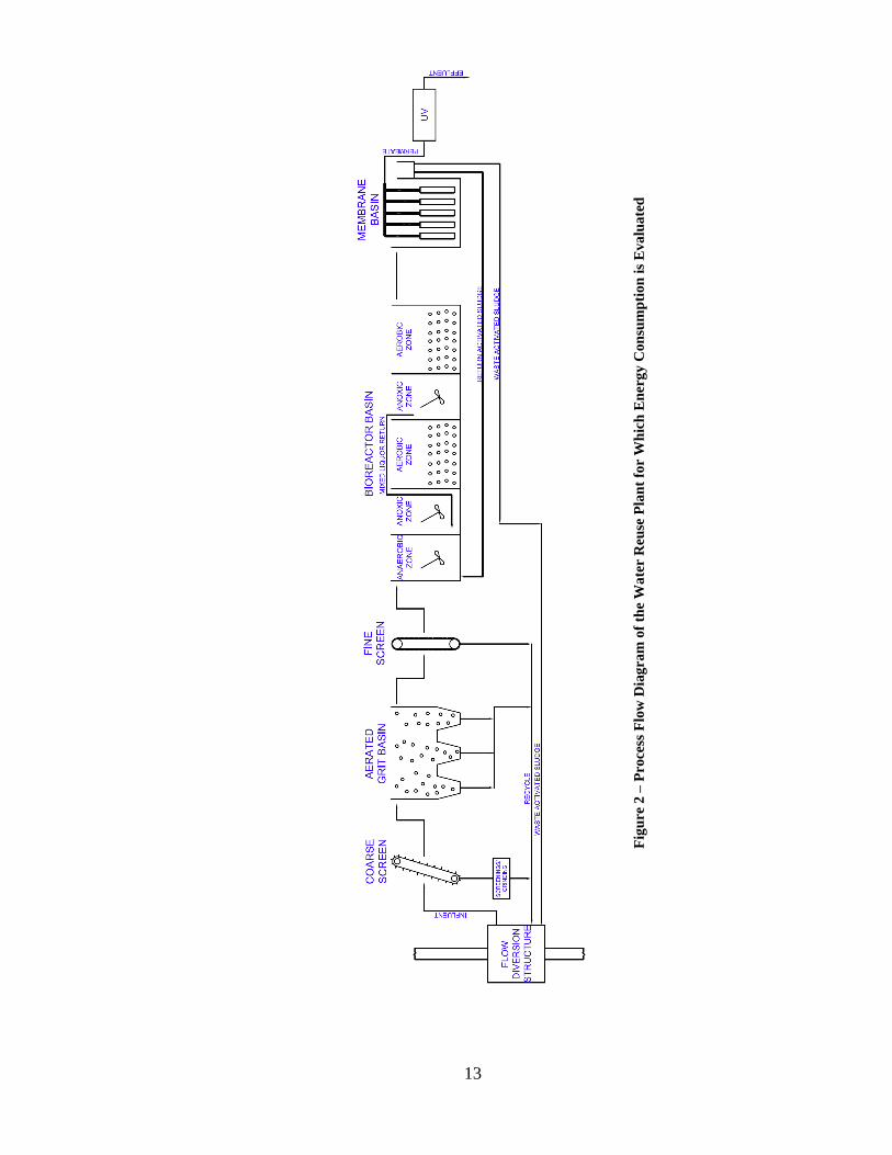
of each process. The process flow diagram of the WRP is shown in Figure 2 and includes,
in order of treatment: coarse screen, aerated grit chambers, fine screen, bioreactor system,
membranes, and UV disinfection. Since there are no solids processing on site, all
screenings, grit, and biosolids are discharged back into the collection sewer trunk. In the
design, a five-stage modified Bardenpho CAS system is provided for the removal of the
nutrients phosphorous and nitrogen (WEF, 2012; WEF, 2011). The design provides for
carbonaceous BOD removal, NH3 oxidation, denitrification through endogenous
respiration, and biological phosphorous removal through PAOs. For this reuse plant,
stringent nutrient removal is required because during winter, when golf course irrigation
needs are less, the effluent could be discharged into an environmentally sensitive lake,
where algal blooms avoidance is a goal. The WRP was designed using design
recommendations and WWTP design equations from various sources (Metcalf & Eddy,
Inc, 2003; WEF, 2010a; Qasim, 1999; Davis, 2010; Lin, 2007; WEF, 2012). The size of
each unit process was determined using Microsoft Excel spreadsheet for the various
scenarios under consideration. Once designed, the energy consuming unit of every unit
process was identified and the expected energy consumption for each unit was computed.
Next, advanced treatment processes were replaced with more traditional unit processes to
evaluate the changes in energy consumption. The MBR system was redesigned to
include a traditional CAS bioreactor with secondary clarification and dual media filters.
Then UV disinfection was replaced with traditional chlorination.
13
Figure 2 – Process Flow Diagram of the Water Reuse Plant for Which Energy Consumption is
Evaluated
Fig
ure
2 –
Pro
cess
Flo
w D
iag
ram
of
the
Wa
ter
Reu
se P
lan
t fo
r W
hic
h E
ner
gy
Con
sum
pti
on
is
Ev
alu
ate
d

14
2.1 Influent and Effluent Quality
The influent characteristics and effluent requirements for the WRP are depicted in
Table 1. The requirements are typical water reuse standards found in California and
Florida (U.S. EPA, 2004a), with the exception for the need to remove nutrients.
Table 1 – Plant Influent and Effluent Process Characteristics Used in the Design
Parameter Influent
Characteristics
Effluent
Requirements
BOD (mg/L) 250 30
TSS (mg/L) 309 30
TKN (mg/L as N) 42 –
NH3 (mg/L as N) 34 0.5
TN (mg/L as N) – 10
TP (mg/L as P) 8 0.2
TC (MPN/100 mL) – 2.2
TC, daily max (MPN/100 mL) – 23
Minimum Temp (°C) 18.3 18.3
2.2 Design Parameters and Considerations
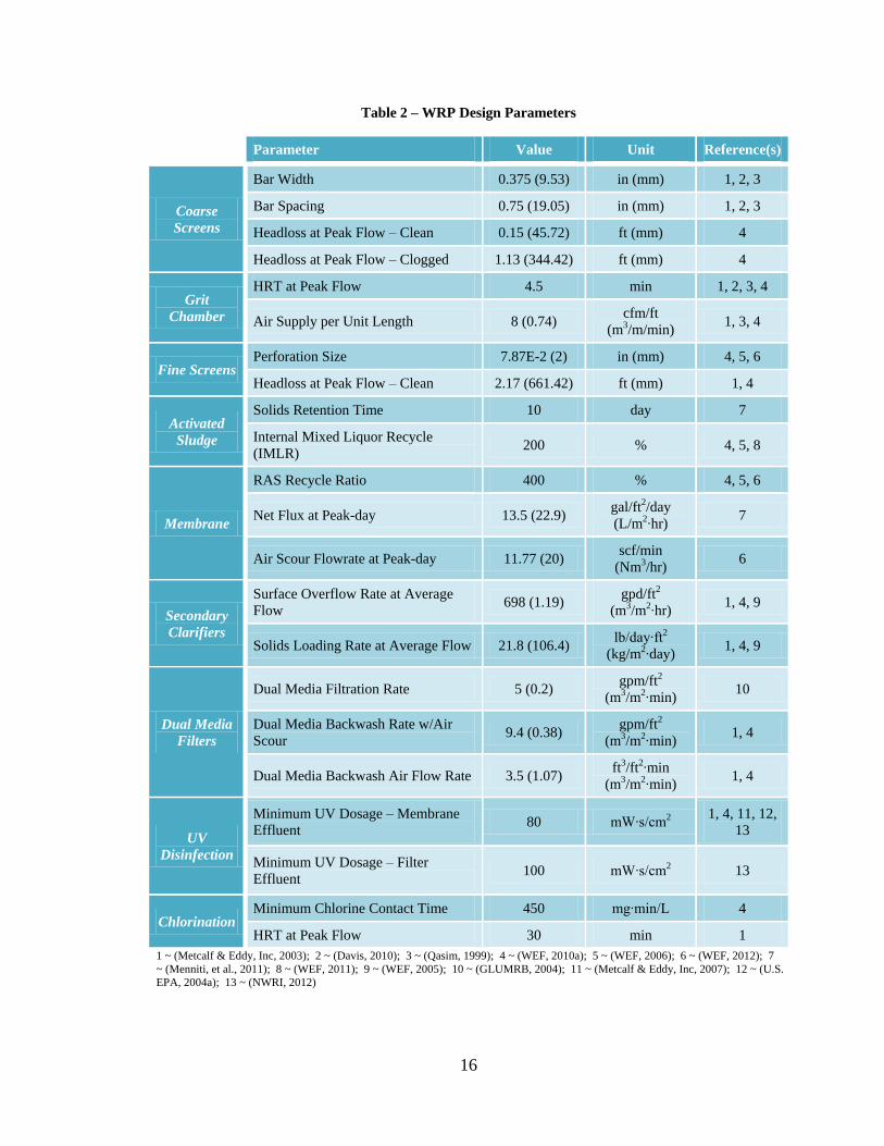
Typical design criteria used to size each unit process are shown in Table 2. Unit
processes included reported in the table include those shown in the process diagram
(Figure 2) and additional ones used for energy consumption comparison. Design values
in the table are typical of values reported in the design literature. All process were
designed taking peak flows into consideration, however, energy consumption
computations are for monthly average flow conditions. A maximum day and peak hour
factors of 1.09 and 1.49 were used in the design, respectively. Peak flows in the facility

15
are to allow for extra capacity during mid day when irrigation cycles happen more
frequently. The designs for each unit process are discussed below. Complete design
methodology and details are found in Appendix A.
16
Table 2 – WRP Design Parameters
Parameter Value Unit Reference(s)
Coarse
Screens
Bar Width 0.375 (9.53) in (mm) 1, 2, 3
Bar Spacing 0.75 (19.05) in (mm) 1, 2, 3
Headloss at Peak Flow – Clean 0.15 (45.72) ft (mm) 4
Headloss at Peak Flow – Clogged 1.13 (344.42) ft (mm) 4
Grit
Chamber
HRT at Peak Flow 4.5 min 1, 2, 3, 4
Air Supply per Unit Length 8 (0.74) cfm/ft
(m3/m/min) 1, 3, 4
Fine Screens Perforation Size 7.87E-2 (2) in (mm) 4, 5, 6
Headloss at Peak Flow – Clean 2.17 (661.42) ft (mm) 1, 4
Activated
Sludge
Solids Retention Time 10 day 7
Internal Mixed Liquor Recycle
(IMLR) 200 % 4, 5, 8
Membrane
RAS Recycle Ratio 400 % 4, 5, 6
Net Flux at Peak-day 13.5 (22.9) gal/ft2/day
(L/m2∙hr) 7
Air Scour Flowrate at Peak-day 11.77 (20) scf/min
(Nm3/hr) 6
Secondary
Clarifiers
Surface Overflow Rate at Average
Flow 698 (1.19)
gpd/ft2
(m3/m2∙hr) 1, 4, 9
Solids Loading Rate at Average Flow 21.8 (106.4) lb/day∙ft2
(kg/m2∙day) 1, 4, 9
Dual Media
Filters
Dual Media Filtration Rate 5 (0.2) gpm/ft2
(m3/m2∙min) 10
Dual Media Backwash Rate w/Air
Scour 9.4 (0.38)
gpm/ft2
(m3/m2∙min) 1, 4
Dual Media Backwash Air Flow Rate 3.5 (1.07) ft3/ft2∙min
(m3/m2∙min) 1, 4
UV
Disinfection
Minimum UV Dosage – Membrane
Effluent 80 mW∙s/cm2
1, 4, 11, 12,
13
Minimum UV Dosage – Filter
Effluent 100 mW∙s/cm2 13
Chlorination Minimum Chlorine Contact Time 450 mg∙min/L 4
HRT at Peak Flow 30 min 1
1 ~ (Metcalf & Eddy, Inc, 2003); 2 ~ (Davis, 2010); 3 ~ (Qasim, 1999); 4 ~ (WEF, 2010a); 5 ~ (WEF, 2006); 6 ~ (WEF, 2012); 7
~ (Menniti, et al., 2011); 8 ~ (WEF, 2011); 9 ~ (WEF, 2005); 10 ~ (GLUMRB, 2004); 11 ~ (Metcalf & Eddy, Inc, 2007); 12 ~ (U.S.
EPA, 2004a); 13 ~ (NWRI, 2012)

17
2.2.1 Influent Channel and Coarse Screens
The design of the rectangular open channel leading to the coarse screens was
based on the Manning’s equation, with a Manning’s coefficient of 0.015 (Sturm, 2010).
Velocity in the designed channel exceeds 1.3 ft/sec (0.4 m/s) during minimum flow to
avoid grit deposition or 3 ft/sec (0.9 m/s) was maintained during peak flows to ensure
resuspension of solids (WEF, 2010a). Key parameters used in the design of the coarse
screens are shown in Table 2. The headloss through the screens was calculated using
both the modified minor loss headloss equation and the Kirshmer’s equation (Metcalf &
Eddy, Inc, 2003; WEF, 2010a). The higher headloss value governed the design. Energy
consumption for the coarse screens is driven by the size of the motor that powers the rake
and the rake cleaning frequency. Based on channel and screen dimensions, a motor size
for the rake was obtained using a graphical method provided by a screen manufacturer
(Vulcan Industries, Inc, 2011).
2.2.2 Aerated Grit Chamber
Parameters used in the design of the aerated grit chamber can be found in Table 2.
The hydraulic retention time (HRT) was determined for the desired peak flowrate with a
depth, width-depth ratio, and length-width ratio chosen in the range of design criteria
(Metcalf & Eddy, Inc, 2003; WEF, 2010a; Qasim, 1999). Energy consumption for the
aerated grit chamber is driven by the air blower capacity used to maintain discrete
particle sedimentation and can be estimated by the following equation (U.S. EPA, 1989):
1/*/428.4283.0 bdas PPeTqEBHP (1)
where BHP = brake horsepower, hp; qs = required flow rate, scfm; Ta = blower inlet air
temperature, °R; e = blower and motor combined efficiency; Pd = blower discharge

18
pressure, psia (the addition of atmospheric pressure and the system head); and Pb = field
atmospheric pressure, psia. System head was estimated as per (U.S. EPA, 1989) using
headloss values for diffuser (0.70 psi; 4.826 kPa), piping (0.15 psi; 1.034 kPa), and inlet
valve and filter headloss (0.30 psi; 2.068 kPa). Atmospheric pressure at 2,000 feet (609.6
meters) elevation was used and a combined blower and motor efficiency of 80% were
assumed (Metcalf & Eddy, Inc, 2003; Davis, 2010).
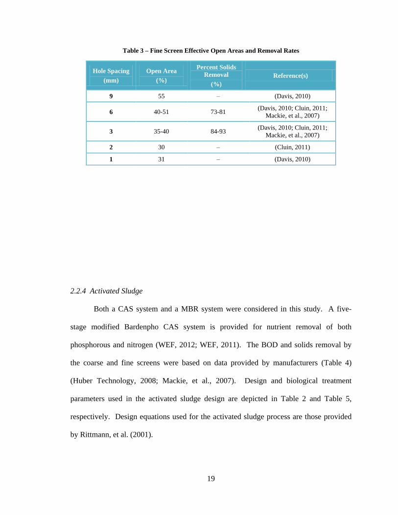
2.2.3 Fine Screens
Design considerations for the open channel preceding the fine screens are the
same as for the open channel before the coarse screens. Parameters used in the design for
the fine screen can be found in Table 2. The headloss across the screen was determined
using the modified orifice headloss equation (Metcalf & Eddy, Inc, 2003; WEF, 2010a).
A blinding factor of up to 50% was applied to determined clogged screen headloss (WEF,
2010a). Typical effective open areas for fine screens and their corresponding solid
removal rates are shown in Table 3. Energy consumption for the fine screens was
computed using the same procedure as for the coarse screens, except that the raking is
continuous.
19
Table 3 – Fine Screen Effective Open Areas and Removal Rates
Hole Spacing
(mm)
Open Area
(%)
Percent Solids
Removal
(%)
Reference(s)
9 55 – (Davis, 2010)
6 40-51 73-81 (Davis, 2010; Cluin, 2011;
Mackie, et al., 2007)
3 35-40 84-93 (Davis, 2010; Cluin, 2011;
Mackie, et al., 2007)
2 30 – (Cluin, 2011)
1 31 – (Davis, 2010)
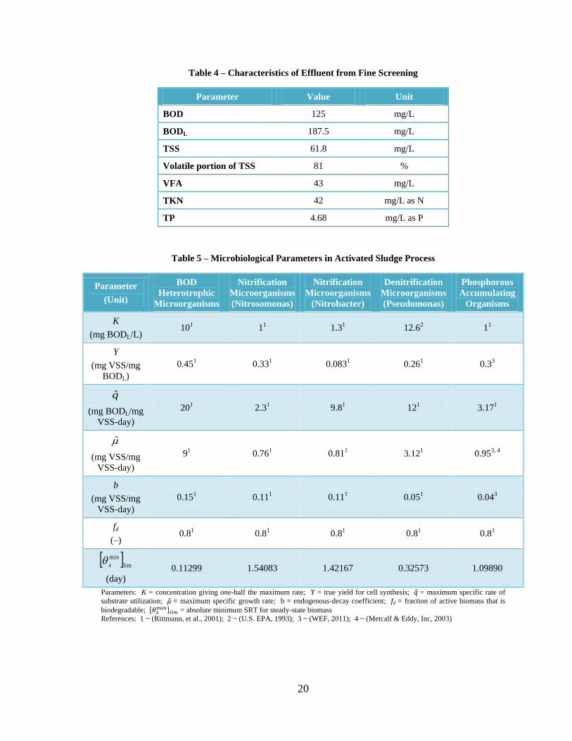
2.2.4 Activated Sludge
Both a CAS system and a MBR system were considered in this study. A five-
stage modified Bardenpho CAS system is provided for nutrient removal of both
phosphorous and nitrogen (WEF, 2012; WEF, 2011). The BOD and solids removal by
the coarse and fine screens were based on data provided by manufacturers (Table 4)
(Huber Technology, 2008; Mackie, et al., 2007). Design and biological treatment
parameters used in the activated sludge design are depicted in Table 2 and Table 5,
respectively. Design equations used for the activated sludge process are those provided
by Rittmann, et al. (2001).
20
Table 4 – Characteristics of Effluent from Fine Screening
Parameter Value Unit
BOD 125 mg/L
BODL 187.5 mg/L
TSS 61.8 mg/L
Volatile portion of TSS 81 %
VFA 43 mg/L
TKN 42 mg/L as N
TP 4.68 mg/L as P
Table 5 – Microbiological Parameters in Activated Sludge Process
Parameter
(Unit)
BOD
Heterotrophic
Microorganisms
Nitrification
Microorganisms
(Nitrosomonas)
Nitrification
Microorganisms
(Nitrobacter)
Denitrification
Microorganisms
(Pseudomonas)
Phosphorous
Accumulating
Organisms
K
(mg BODL/L) 101 11 1.31 12.62 11
Y
(mg VSS/mg
BODL)
0.451 0.331 0.0831 0.261 0.33
q
(mg BODL/mg
VSS-day)
201 2.31 9.81 121 3.171
(mg VSS/mg
VSS-day)
91 0.761 0.811 3.121 0.953, 4
b
(mg VSS/mg
VSS-day)
0.151 0.111 0.111 0.051 0.043
fd
(–) 0.81 0.81 0.81 0.81 0.81
lim
min
x
(day) 0.11299 1.54083 1.42167 0.32573 1.09890
Parameters: K = concentration giving one-half the maximum rate; Y = true yield for cell synthesis; = maximum specific rate of
substrate utilization; = maximum specific growth rate; b = endogenous-decay coefficient; fd = fraction of active biomass that is
biodegradable; [ ] = absolute minimum SRT for steady-state biomass
References: 1 ~ (Rittmann, et al., 2001); 2 ~ (U.S. EPA, 1993); 3 ~ (WEF, 2011); 4 ~ (Metcalf & Eddy, Inc, 2003)
21
In an activated sludge MBR system, return activated sludge (RAS) rates are
typically higher compared to CAS process. For a MBR system, RAS rates are typically
200 to 500% of the average influent flow, versus 50 to 100% in CAS systems (WEF,
2012; WEF, 2010a; WEF, 2006). These systems also require a higher MLSS
concentration compared to CAS systems. For a MBR system, the MLSS concentration
inside the bioreactor tank can be between 4,000 to 10,000 mg/L and inside the membrane
tank 8,000 to 18,000 mg/L, versus 1,500 to 3,500 mg/L in CAS systems (WEF, 2012;
WEF, 2006; WEF, 2010a). Due to these higher MLSS concentrations (Fabiyi, et al.,
2008), a decreased alpha factor, or oxygen transfer efficiency of diffused air, of 0.5
results for MBR facilities with MLSS concentrations around 10,000 mg/L (Germain, et
al., 2007). For CAS facilities with nitrification and denitrification, an alpha factor of 0.7
was used (Rosso, et al., 2006). The alpha factor is not only affected by solid
concentrations inside the basin but also the type of treatment, due to low molecular
weight surfactant uptake in the anoxic zone (Rosso, et al., 2006). Energy consumption
for the activated sludge process is driven by mixers used to maintain particles suspension
in the anaerobic and anoxic zones of the biological nutrient removal system, and blowers
used to provide oxygen and particle suspension in the aerated zones. In addition, energy
is required to operate the IMLR pumps and RAS pumps. Mixer energy requirement was
determined based on the basin volume and the type of mixer. For horizontal mixers the
required energy used was 7 W/m3 (WEF, 2010a). Blower energy was determined using
equation 1 and a combined blower and motor efficiency of 80% (Metcalf & Eddy, Inc,
2003; Davis, 2010). Energy requirements for pumps after they have been sized were
determined as (Jones, et al., 2008):

22
pE
qHBHP
3960 (2)
where BHP = brake horsepower, hp; q = required flow rate, gal/min; H = total dynamic
head, ft; and Ep = pump efficiency. Efficiencies for both the IMLR and RAS pumps
were chosen in ranges from pump data and curves. A pump efficiency of 80% was used
for both pumps (Goulds Pumps, 2012).
2.2.5 Membranes
Parameters used in the design of the membrane portion of the MBR system can be
found in Table 2. MLSS concentration inside the membrane tank was determined as per
(WEF, 2012). The required membrane area needed inside the tank was determined using
the net flux concept (WEF, 2012). Typical membrane parameters including membrane
area per small subunit, number of small subunits per large subunit, and volume required
per large subunits (WEF, 2012). The air scour cycle rates during average and peak-day
flowrates were 10 sec on/30 sec off and 10/10, respectively (WEF, 2012). An online
factor of 95% percent was also used to allow for relaxation intervals and maintenance
cleaning (WEF, 2012). Energy consumption for the membranes is driven by air scour
blowers, permeate pumps, backpulse pumps, and WAS pumps. The consumption of
energy was calculated for the blower and pumps using equations 1 and 2, respectively.
The combined and pump efficiencies used for both the blower and WAS pumps,
respectively, were 80% (Metcalf & Eddy, Inc, 2003; Davis, 2010), and the pump
efficiencies used for permeate and backpulse pumps were 70% (Goulds Pumps, 2012).
2.2.6 Secondary Clarifier
The alternative biological process used to contrast a MBR system was a
traditional CAS system. The biological portion of the design is the same as for the MBR
23
system, except for the MLSS concentration, RAS ratio, and alpha factor as discussed
above. This would require a doubling in aeration volume compared to the MBR system’s
biological process. The membranes are replaced with secondary clarification and
filtration to provide solid separation. Parameters used in the design of the secondary
clarifier can be found in Table 2. The clarifier was sized using recommended overflow
rates and solids loading rates as per (Metcalf & Eddy, Inc, 2003; WEF, 2010a; WEF,
2005). Design was performed for both peak and average flow, with the highest value
governing the design. Weir loading was checked for both average and peak flows to
ensure the loadings were under recommended limits (WEF, 2005; WEF, 2010a). Energy
consumption for the secondary clarifier is driven by the size of the motor that provides
the torque for the rake arm and the WAS pump. The required power to move the rake
arm was calculated using (WEF, 2005):
TP (3)
where P = power required by the motor, W; T = required torque, J, T = Wr2 where W =
rake arm loading, N/m and r = radius of rake arm, m; and ω = angular velocity, rad/s. A
rake arm loading value of 95 N/m was used and fell within the recommended range for
secondary sludge (WEF, 2005). The energy requirement for the WAS pump was
determined using equation 2. A pump efficiency of 80% was used (Goulds Pumps, 2012).
2.2.7 Dual Media Filters
Parameters used in the design of the dual media filters can be found in Table 2.
The number and size of the filters were determined using (WEF, 2010a) and the filtration
rate (GLUMRB, 2004). Filter sizes were rounded to the nearest increment of 25 square
feet to allow for ease of construction. The filters were designed with one filter out of
24
service for backwashing cycles. The cleanwater headlosses were determined to be 0.81
and 1.45 feet for average and peak filtration rates, respectively, using the Rose equation
(Metcalf & Eddy, Inc, 2003). Backwash cycles were design to be 36 hours, determined
using solids holding capacity for clogged headloss determination (Metcalf & Eddy, Inc,
2003; WEF, 2010a). Energy consumption for the dual media filters is driven by the
backwash blower and backwash pump, equations 1 and 2. A combined blower and motor
efficiency of 80% was used for the backwash blower (Metcalf & Eddy, Inc, 2003) and a
pump efficiency of 78% was used for the backwash pump (Goulds Pumps, 2012).
2.2.8 UV Disinfection
The parameters used in the design of the UV disinfection process can be found in
Table 2. Two UV disinfection system designs were considered, low and medium-
pressure. When designing the UV disinfection system with low-pressure UV lamps, a
graphical point-source-summation method was used to determine the water quality factor
and the effluent coliform number, using suspended solids concentrations and UV dosage,
respectively (WEF, 2010a; U.S. EPA, 1986). Low-pressure high intensity lamps were
assumed to have a maximum input power of 260 W with an efficiency of 33% (Metcalf
& Eddy, Inc, 2003; Trojan Technologies, 2008). The variable output (dimming)
capabilities of this lamp are from 60 to 100% (Trojan Technologies, 2008). For medium-
pressure UV lamps, an equation based point-source-summation was performed for
estimating the UV intensity (U.S. EPA, 1986). The required UV dose was determined as
per (WEF, 2010a). To determine the effluent coliform number after exposure, a variation
of the Chick-Watson first-order model was used (Metcalf & Eddy, Inc, 2003; WEF,
2010a; U.S. EPA, 1986). Medium-pressure high intensity were assumed having a
25
maximum input power of 3,200 W with an efficiency of 12% (Metcalf & Eddy, Inc,
2003; Trojan Technologies, 2007). The variable output capabilities of this lamp are from
30 to 100% (Trojan Technologies, 2007). The headloss through the UV channel was
determined using the energy equation from (Metcalf & Eddy, Inc, 2003; Qasim, 1999).
2.2.9 Chlorination
The alternative disinfection process used to contrast UV disinfection was
chlorination. Chlorination would follow membranes in the MBR facility and the dual
media filters in the CAS facility. Parameters used in the design of the chlorination
contact basin are depicted in Table 2. The chlorine dosage was determined using a
modification of the Collins-Selleck model found in (Metcalf & Eddy, Inc, 2003).
Membrane effluent total coliform bacterium has a typical range of 10 to 1000
MPN/100mL (Metcalf & Eddy, Inc, 2003; DeCarolis Jr, et al., 2007) and filter effluent
total coliform bacterium has a typical range of 104 to 10
6 MPN/100mL (Metcalf & Eddy,
Inc, 2003). The design assumed a chlorine residual of 3 mg/L leaving the facility.
Dechlorination was not considered in this design because water is to be used for golf
course irrigation. With a design scheme layout of the chlorine contact basin determined
and sized, proper dispersion was evaluated using the axial dispersion equations found in
Metcalf & Eddy, Inc (2003). Energy consumption for chlorination is driven by the size
of the diaphragm pump used to inject chlorine before the contact basin. This energy
requirement can be calculated using equation 2. A pump efficiency of 70% was used
(Goulds Pumps, 2012).

26
3. Results and Analysis
Estimated energy consumption for major energy driving units of each process and
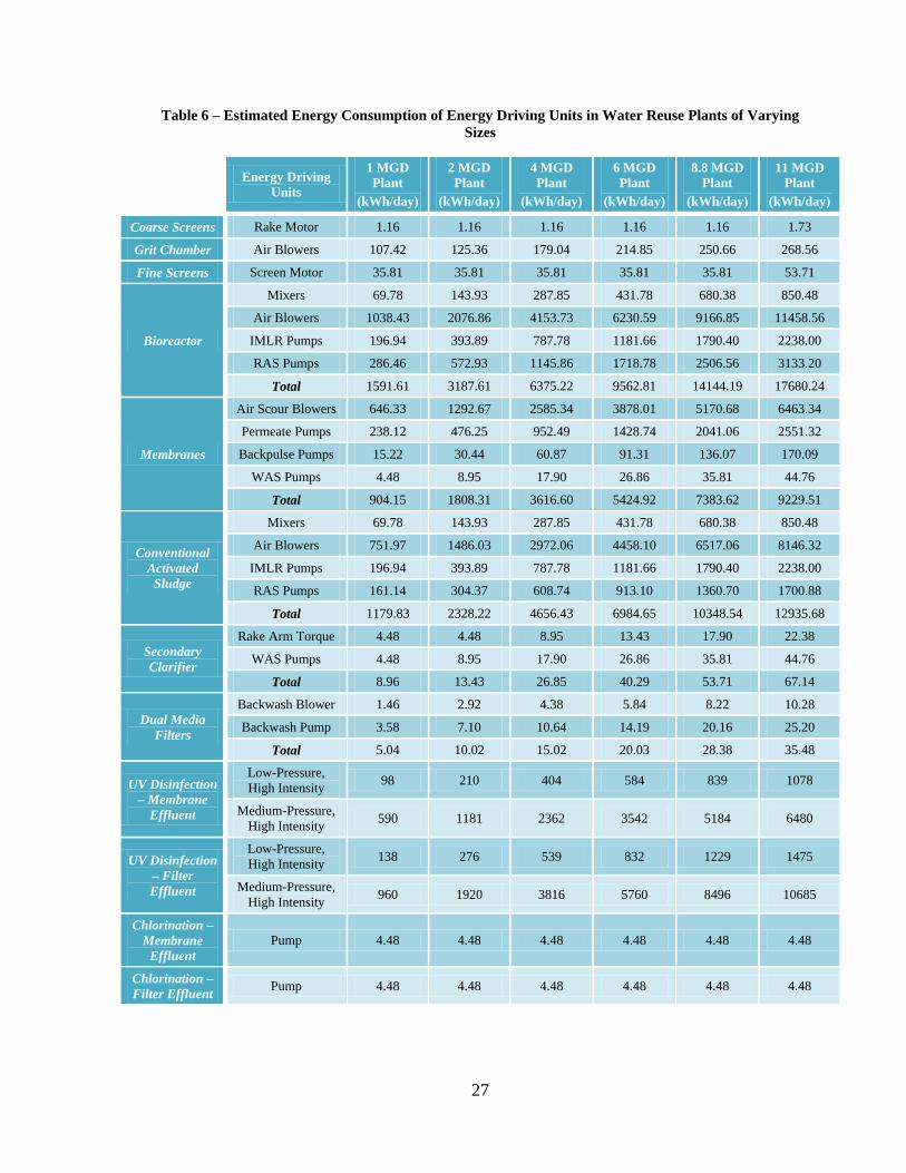
for varying WRP flowrates are shown in Table 6.
27
Table 6 – Estimated Energy Consumption of Energy Driving Units in Water Reuse Plants of Varying
Sizes
Energy Driving
Units
1 MGD
Plant
(kWh/day)
2 MGD
Plant
(kWh/day)
4 MGD
Plant
(kWh/day)
6 MGD
Plant
(kWh/day)
8.8 MGD
Plant
(kWh/day)
11 MGD
Plant
(kWh/day)
Coarse Screens Rake Motor 1.16 1.16 1.16 1.16 1.16 1.73
Grit Chamber Air Blowers 107.42 125.36 179.04 214.85 250.66 268.56
Fine Screens Screen Motor 35.81 35.81 35.81 35.81 35.81 53.71
Bioreactor
Mixers 69.78 143.93 287.85 431.78 680.38 850.48
Air Blowers 1038.43 2076.86 4153.73 6230.59 9166.85 11458.56
IMLR Pumps 196.94 393.89 787.78 1181.66 1790.40 2238.00
RAS Pumps 286.46 572.93 1145.86 1718.78 2506.56 3133.20
Total 1591.61 3187.61 6375.22 9562.81 14144.19 17680.24
Membranes
Air Scour Blowers 646.33 1292.67 2585.34 3878.01 5170.68 6463.34
Permeate Pumps 238.12 476.25 952.49 1428.74 2041.06 2551.32
Backpulse Pumps 15.22 30.44 60.87 91.31 136.07 170.09
WAS Pumps 4.48 8.95 17.90 26.86 35.81 44.76
Total 904.15 1808.31 3616.60 5424.92 7383.62 9229.51
Conventional
Activated
Sludge
Mixers 69.78 143.93 287.85 431.78 680.38 850.48
Air Blowers 751.97 1486.03 2972.06 4458.10 6517.06 8146.32
IMLR Pumps 196.94 393.89 787.78 1181.66 1790.40 2238.00
RAS Pumps 161.14 304.37 608.74 913.10 1360.70 1700.88
Total 1179.83 2328.22 4656.43 6984.65 10348.54 12935.68
Secondary
Clarifier
Rake Arm Torque 4.48 4.48 8.95 13.43 17.90 22.38
WAS Pumps 4.48 8.95 17.90 26.86 35.81 44.76
Total 8.96 13.43 26.85 40.29 53.71 67.14
Dual Media
Filters
Backwash Blower 1.46 2.92 4.38 5.84 8.22 10.28
Backwash Pump 3.58 7.10 10.64 14.19 20.16 25.20
Total 5.04 10.02 15.02 20.03 28.38 35.48
UV Disinfection
– Membrane
Effluent
Low-Pressure,
High Intensity 98 210 404 584 839 1078
Medium-Pressure,
High Intensity 590 1181 2362 3542 5184 6480
UV Disinfection
– Filter
Effluent
Low-Pressure,
High Intensity 138 276 539 832 1229 1475
Medium-Pressure,
High Intensity 960 1920 3816 5760 8496 10685
Chlorination –
Membrane
Effluent
Pump 4.48 4.48 4.48 4.48 4.48 4.48
Chlorination –
Filter Effluent Pump 4.48 4.48 4.48 4.48 4.48 4.48

28
Preliminary and Primary Treatment Units
Preliminary and primary treatment units include coarse screens, aerated grit
chamber, and fine screens. The energy consumption by the fine screens in the reuse
plants are about thirty-one times that consumed by the coarse screens, due to the fine
screens being continuously run. However, the energy consumed by both screens is small
relative to that consumed by other unit processes. On average, both screens together
require 0.72% of the plant’s total energy consumption. For flowrates varying from 1 to
8.8 MGD (Figure 3a), energy consumption for both processes are constant until a
flowrate above 8.8 MGD is reached. This is the case because in order to remove large
debris from screens a minimum motor size must be used, independent of the flowrate
(Vulcan Industries, Inc, 2011). The Water Environment Federation (WEF, 2010b)
reports energy consumption for coarse screens are equal to 2 kWh/d for flows between 1
to 10 MGD and increases at larger flows (WEF, 2010b). In this research, values of 1.16
to 1.73 kWh/day were found and are similar to the values and pattern reported by WEF,
2010b. Malcolm Pirnie (1995) reports that a 0.39 MGD facility uses 17.53 kWh/day for
fine screens and 96.89 kWh/day for a 2.85 MGD facility. A value of 35.81 kWh/day was
found in this research at 1 MGD, which is roughly two times the value found at the 0.39
MGD facility.
The energy consumption in the aerated grit chamber is a function of flowrate
treated and it increases initially and tapers down resulting in a decreasing slope as flow
increases (Figure 3b). This behavior occurs due to the chosen design depth used in the
chamber. Design depth increases rapidly at lower flow ranges, 1 – 4 MGD, and begins to
steady at flow ranges above 6 MGD; indicating depth is directly related to the energy
29
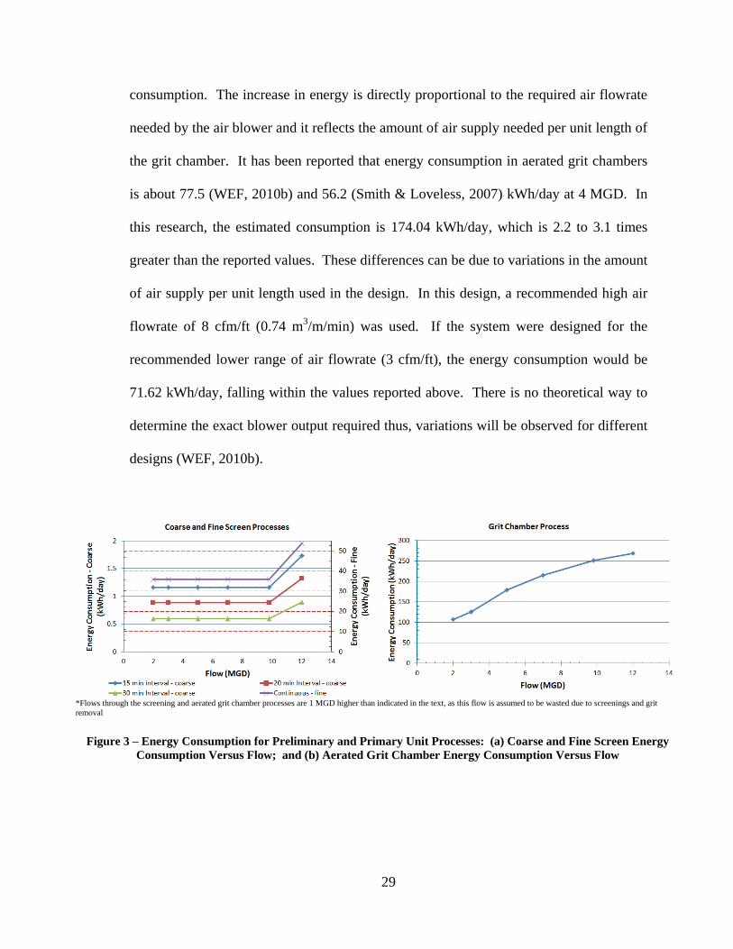
consumption. The increase in energy is directly proportional to the required air flowrate
needed by the air blower and it reflects the amount of air supply needed per unit length of
the grit chamber. It has been reported that energy consumption in aerated grit chambers
is about 77.5 (WEF, 2010b) and 56.2 (Smith & Loveless, 2007) kWh/day at 4 MGD. In
this research, the estimated consumption is 174.04 kWh/day, which is 2.2 to 3.1 times
greater than the reported values. These differences can be due to variations in the amount
of air supply per unit length used in the design. In this design, a recommended high air
flowrate of 8 cfm/ft (0.74 m3/m/min) was used. If the system were designed for the
recommended lower range of air flowrate (3 cfm/ft), the energy consumption would be
71.62 kWh/day, falling within the values reported above. There is no theoretical way to
determine the exact blower output required thus, variations will be observed for different
designs (WEF, 2010b).
*Flows through the screening and aerated grit chamber processes are 1 MGD higher than indicated in the text, as this flow is assumed to be wasted due to screenings and grit
removal
Figure 3 – Energy Consumption for Preliminary and Primary Unit Processes: (a) Coarse and Fine Screen Energy
Consumption Versus Flow; and (b) Aerated Grit Chamber Energy Consumption Versus Flow
30
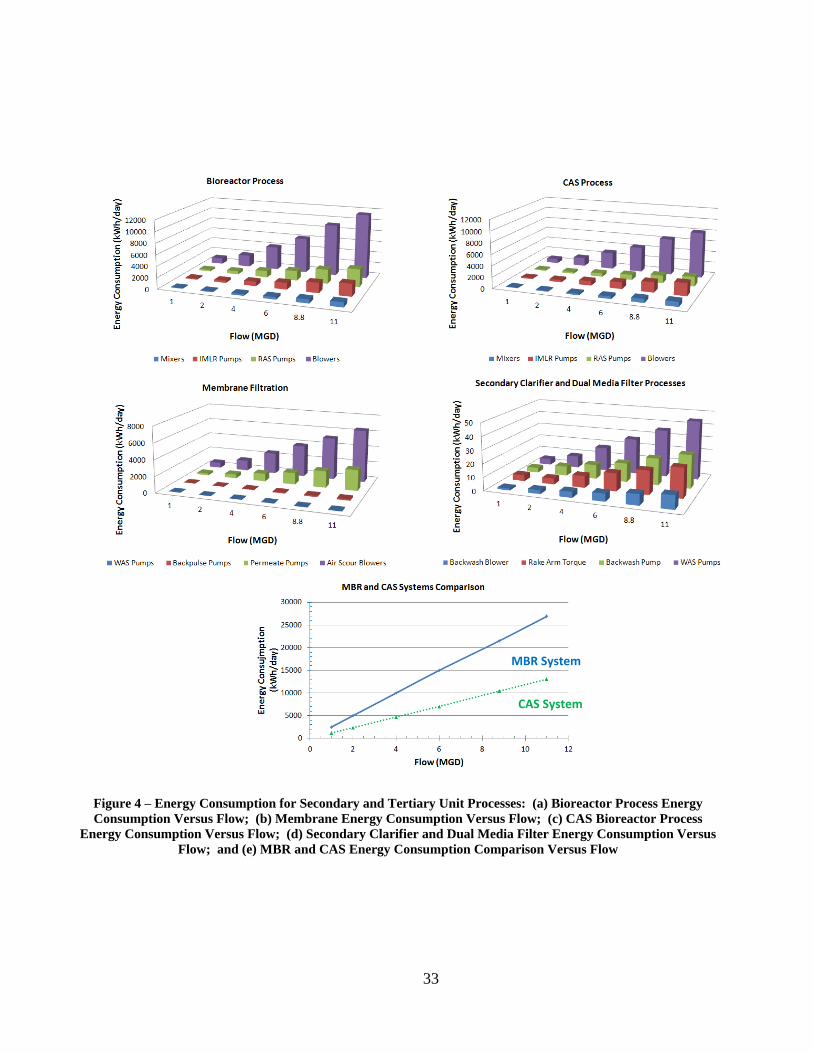
Secondary and Tertiary Treatment Units
Secondary and tertiary treatment units include: bioreactor and membrane filters
for a MBR facility; and CAS bioreactor process, secondary clarifier, and dual media
filters for a CAS facility. The energy consumption for secondary and tertiary treatment
unit processes are shown in Figure 4a to 3d. The air requirements in the basins were
estimated as 1,038.43 kWh/day at 1 MGD for a MBR facility and 751.97 kWh/day for a
CAS facility. At this same flowrate WEF (2010b) reports a value of 878 kWh/day, which
is about 15.4% lower than the value estimated by this research for the MBR facility and
14.4% higher for the CAS facility. It is known that energy consumption in biological
treatment units is affected by wastewater strength (i.e. BOD and ammonia loadings).
However, in this research, the impacts of wastewater loading on energy consumption in
the bioreactors were not evaluated. Therefore, comparisons with reported literature are
based on flowrates only. For flowrates between 1 – 11 MGD, the energy consumption of
the air blowers on average was 65.1% of the total biological process energy consumption
for MBR facilities and 63.5% for CAS facilities. IMLR and RAS pumps required 12.5
and 17.9% of the total biological energy consumption for the MBR facilities and 17.0 and
13.2% for CAS facilities. Aerobic and anoxic mixers were on average 4.6% for MBR
and 6.7% for CAS. In comparing the biological bioreactor process and CAS bioreactor
process, the difference in energy consumptions relates mainly to the RAS pumps and air
blowers. It was estimated that the RAS pumps required 2,506.56 and 1,360.70 kWh/day
of energy for MBR and CAS facilities at 8.8 MGD, respectively (Table 6). The higher
energy consumption for MBR facilities is due to the high recycle rates needed in the
31
MBR process. In CAS facilities, the high energy consumption is dependent of the TDH
difference related to the position of the RAS pumps and the clarifiers; however, the
impact of the recycle in the MBR process is much greater. For flowrates between 1 – 11
MGD, the MBR facilities were found on average to require 1.85 times more consumption
of energy in RAS pumping. The air blowers at 8.8 MGD required 9,166.85 kWh/day for
MBR facilities and 6,517.06 kWh/day for CAS facilities. This increase for MBR
facilities was on average 1.4 times the amount of energy needed at CAS facilities. This is
a result of a decreased alpha factor (oxygen transfer efficiency of diffused air) of 0.5
(Germain, et al., 2007) in MBR facilities, as compared to 0.7 (Rosso, et al., 2006) in CAS
facilities. The different alpha factor is a result of the higher solids concentrations
maintained in MBRs (Fabiyi, et al., 2008).
Comparing the membrane with the secondary clarifier and dual media filter for
secondary filtration, it can be observed that the membrane process requires a very large
amount of energy (7,383.61 kWh/day), while the secondary clarifier and dual media filter
processes requires less (82.09 kWh/day) at 8.8 MGD, which comprises about 1% of that
consumed by the membrane process for flowrates between 1 – 11 MGD on average. The
reason for this is due to the required pumping and blowers needed to run and maintain the
membrane system (Figure 4b and 3d). Air scour blowers and permeate and backpulse
pumps require 71.0 and 28.5%, respectively, of the total membrane energy consumption.
WAS pumps only require a consumption of 0.5%. For secondary clarifier and dual media
filter energy consumption, the largest contributor was the WAS pumps requiring an
average of 40.8% of the total consumption across all flows. The secondary clarifier rake
32
arm and the dual media filter backwash pumps both require about 25% of the total energy
consumption.
The overall energy consumption for each system train, MBR and CAS is depicted
in Figure 4e. It is observed that the MBR process, on average for the flow ranges
investigated, is 2.10 times more energy intensive than the traditional CAS process.
Reports on MBR energy consumption say MBR energy may be twice that of CAS (WEF,
2010b; U.S. EPA, 2010) to as much as three times (Wallis-Lage, et al., 2011). As
observed in Figure 4e, energy consumption is directly proportional to the influent
flowrate for both MBR and CAS with secondary filtration processes. For instance at 2
MGD, energy consumption is 4,996 kWh/day while at 6 MGD the consumption of
energy is 14,988 kWh/day, which is three times more energy intensive. The largest
energy consuming unit in the MBR process is air scouring and it accounts for 23.7% of
the total energy demand of the entire plant across all flows. This is contrasted to 35 to
40% found in (WEF, 2010b; U.S. EPA, 2010; DeCarolis, et al., 2008).
33
Figure 4 – Energy Consumption for Secondary and Tertiary Unit Processes: (a) Bioreactor Process Energy
Consumption Versus Flow; (b) Membrane Energy Consumption Versus Flow; (c) CAS Bioreactor Process
Energy Consumption Versus Flow; (d) Secondary Clarifier and Dual Media Filter Energy Consumption Versus
Flow; and (e) MBR and CAS Energy Consumption Comparison Versus Flow
MBR System
CAS System

34
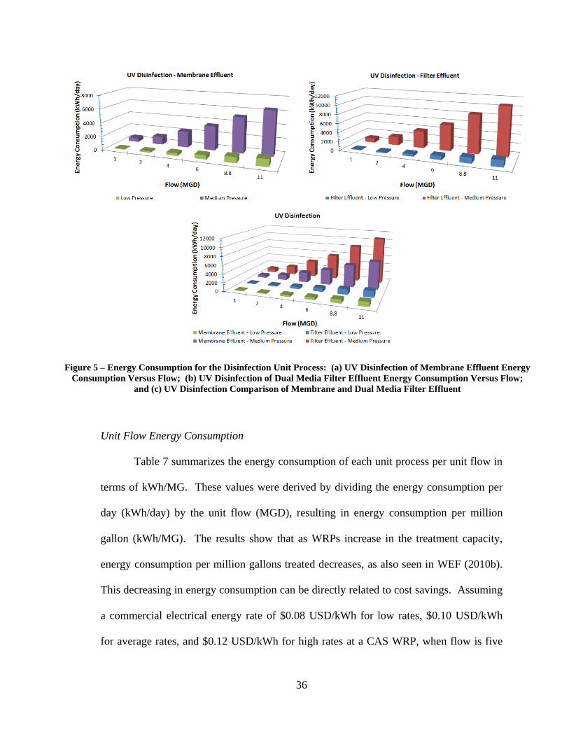
Disinfection Units
Disinfection methods considered include UV disinfection and chlorination. The
energy consumption in terms of flowrate for the UV disinfection process for both low and
medium pressure lamps is shown in Figure 5. For low and medium-pressure high
intensity lamps, energy consumption increases with flowrate. This increase is directly
proportional to the flow. Slight variations in energy consumption of both low and
medium-pressure lamps is due to the number of lamps that can be in a module and the
number of modules that can be in a bank per UV channel (Trojan Technologies, 2007;
Trojan Technologies, 2008). Therefore, the exact dosage varied slightly at different
flowrates. Studies have found that UV disinfection can take up approximately 10 to 25%
of a facility’s total energy consumption (U.S. EPA, 2010). In this research, it was found
that UV disinfection for all flows had on average a 3.7 and 9.9% total energy
consumption for MBR and CAS treatment facilities with low pressure lamps,
respectively; and 18.8 and 43.6% with medium pressure lamps. It is observed that filter
effluent requires more energy for disinfection compared to membrane effluent due to the
higher MPN and TSS levels in the filter effluent, as well as the higher dosage
requirement. For instance at 6 MGD, membrane effluent requires 584 and 3,542
kWh/day for low-pressure and medium-pressure lamps, respectively, while the filter
effluent requires 832 and 5,760 kWh/day. On average across all flows, filter effluent
requires a 38.6% increase in energy consumption for low-pressure lamps and 63.0%
increase for medium-pressure lamps.
In the research, results indicate that medium-pressure high intensity lamps
required more energy to disinfect compared to low-pressure high intensity lamps. On
35
average for membrane effluent, medium-pressure lamps required a 5.96 times increase in
energy consumption compared to low-pressure. For filter effluent, a 7.01 times increase
is also observed. These results are consistent with reports on low-pressure lamps
requiring less energy to deliver the same UV dose compared to medium-pressure lamps
(WEF, 2010b). As energy consumption is directly proportional to the flowrate being
treated, the energy gap between the low and medium pressure lamps stays constant as
flows change. URS (2004) reports that at a 18 MGD facility, low-pressure high intensity
lamps require 1,080 kWh/day and medium-pressure high intensity lamps require 4,560
kWh/day; resulting in an energy gap of 4.22 times between low and medium-pressure
lamps. For this reason, in this study total facility energy calculations incorporate low-
pressure lamps. It is well known that UV disinfection is an energy intensive process,
especially when compared to chlorination (WEF, 2010b; Metcalf & Eddy, Inc, 2003).
Chlorination energy consumption stayed constant for both MBR and CAS facility flows.
This occurs because the pump motor size used stayed the same (0.25 hp) to allow
sufficient power to overcome greater pressure heads at higher flows. This additional
power allows for sufficient mixing energy. Chlorination on average was only 1% of the
total energy consumed when compared to UV disinfection.
36
Figure 5 – Energy Consumption for the Disinfection Unit Process: (a) UV Disinfection of Membrane Effluent Energy
Consumption Versus Flow; (b) UV Disinfection of Dual Media Filter Effluent Energy Consumption Versus Flow;
and (c) UV Disinfection Comparison of Membrane and Dual Media Filter Effluent
Unit Flow Energy Consumption
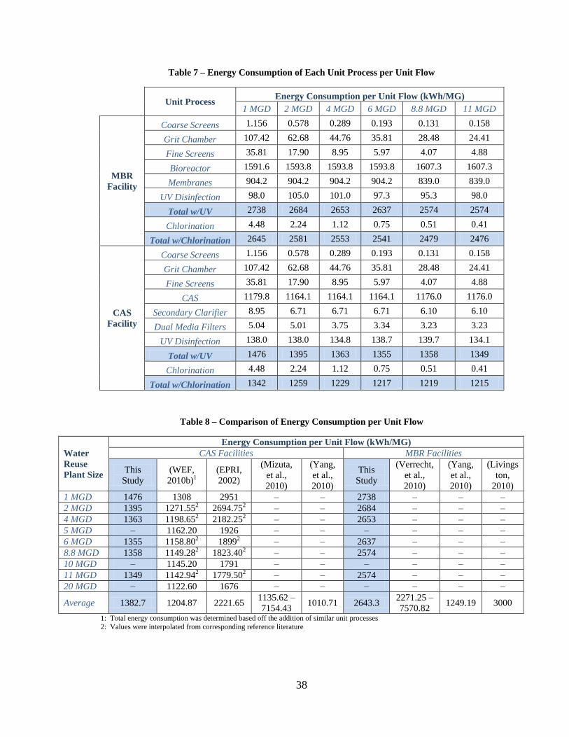
Table 7 summarizes the energy consumption of each unit process per unit flow in
terms of kWh/MG. These values were derived by dividing the energy consumption per
day (kWh/day) by the unit flow (MGD), resulting in energy consumption per million
gallon (kWh/MG). The results show that as WRPs increase in the treatment capacity,
energy consumption per million gallons treated decreases, as also seen in WEF (2010b).
This decreasing in energy consumption can be directly related to cost savings. Assuming
a commercial electrical energy rate of $0.08 USD/kWh for low rates, $0.10 USD/kWh
for average rates, and $0.12 USD/kWh for high rates at a CAS WRP, when flow is five
37
times as large compared to a 1 MGD facility, the savings in energy costs is $7.44/MG
treated at low rates, $9.30/MG treated at average rates, and $11.16/MG treated at high
rates; and $13.12/MG, $16.40/MG, $19.68/MG treated at ten times the flow for low,
average, and high energy rates. Table 7 can be used in targeting unit processes that are in
need of minimizing energy consumption. In addition, the table can be used as a basis for
decision making regarding sustainability of using advanced treatment technologies in
reuse plants.
The resulting values for the CAS and MBR facilities along with published values
for energy consumption in WWTPs are shown in Table 8. For the 1 MGD CAS facility,
the energy consumed was found to be 1,476 kWh/MG in this research. This value is
50.0% smaller than values for the same flowrate reported by EPRI (2002), 2,951
kWh/MG, and it is 12.8% greater than values reported by WEF (2010b), 1,308 kWh/MG.
On average, energy consumption for the designed MBR facilities were determined to be
2,643 kWh/MG and is comparable to reported values for typical MBR facilities with an
energy consumption of 3,000 kWh/MG (Livingston, 2010). This research found that the
MBR WRP is on average 1.91 times more energy intensive than the CAS WRP.
38
Table 7 – Energy Consumption of Each Unit Process per Unit Flow
Unit Process
Energy Consumption per Unit Flow (kWh/MG)
1 MGD 2 MGD 4 MGD 6 MGD 8.8 MGD 11 MGD
MBR
Facility
Coarse Screens 1.156 0.578 0.289 0.193 0.131 0.158
Grit Chamber 107.42 62.68 44.76 35.81 28.48 24.41
Fine Screens 35.81 17.90 8.95 5.97 4.07 4.88
Bioreactor 1591.6 1593.8 1593.8 1593.8 1607.3 1607.3
Membranes 904.2 904.2 904.2 904.2 839.0 839.0
UV Disinfection 98.0 105.0 101.0 97.3 95.3 98.0
Total w/UV 2738 2684 2653 2637 2574 2574
Chlorination 4.48 2.24 1.12 0.75 0.51 0.41
Total w/Chlorination 2645 2581 2553 2541 2479 2476
CAS
Facility
Coarse Screens 1.156 0.578 0.289 0.193 0.131 0.158
Grit Chamber 107.42 62.68 44.76 35.81 28.48 24.41
Fine Screens 35.81 17.90 8.95 5.97 4.07 4.88
CAS 1179.8 1164.1 1164.1 1164.1 1176.0 1176.0
Secondary Clarifier 8.95 6.71 6.71 6.71 6.10 6.10
Dual Media Filters 5.04 5.01 3.75 3.34 3.23 3.23
UV Disinfection 138.0 138.0 134.8 138.7 139.7 134.1
Total w/UV 1476 1395 1363 1355 1358 1349
Chlorination 4.48 2.24 1.12 0.75 0.51 0.41
Total w/Chlorination 1342 1259 1229 1217 1219 1215
Table 8 – Comparison of Energy Consumption per Unit Flow
Water
Reuse
Plant Size
Energy Consumption per Unit Flow (kWh/MG)
CAS Facilities MBR Facilities
This
Study
(WEF,
2010b)1
(EPRI,
2002)
(Mizuta,
et al.,
2010)
(Yang,
et al.,
2010)
This
Study
(Verrecht,
et al.,
2010)
(Yang,
et al.,
2010)
(Livings
ton,
2010)
1 MGD 1476 1308 2951 – – 2738 – – –
2 MGD 1395 1271.552 2694.752 – – 2684 – – –
4 MGD 1363 1198.652 2182.252 – – 2653 – – –
5 MGD – 1162.20 1926 – – – – – –
6 MGD 1355 1158.802 18992 – – 2637 – – –
8.8 MGD 1358 1149.282 1823.402 – – 2574 – – –
10 MGD – 1145.20 1791 – – – – – –
11 MGD 1349 1142.942 1779.502 – – 2574 – – –
20 MGD – 1122.60 1676 – – – – – –
Average 1382.7 1204.87 2221.65 1135.62 –
7154.43 1010.71 2643.3
2271.25 –
7570.82 1249.19 3000
1: Total energy consumption was determined based off the addition of similar unit processes
2: Values were interpolated from corresponding reference literature

39
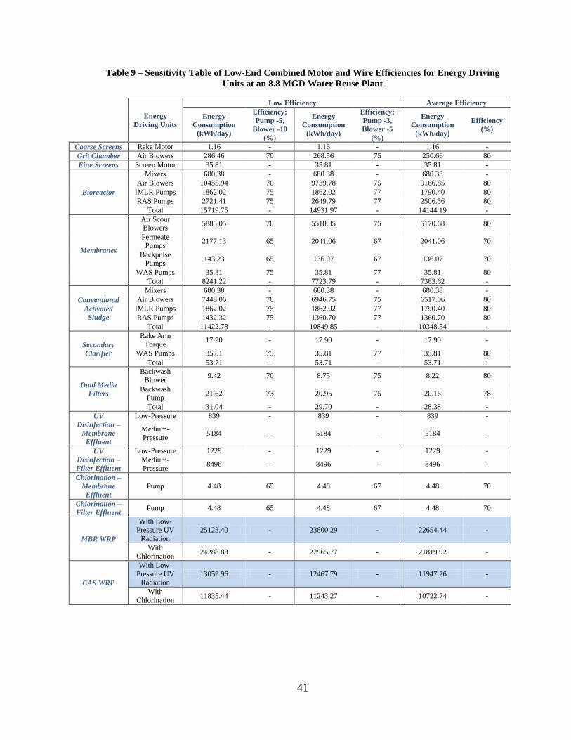
The efficiencies considered in the energy computations are a combined motor and
equipment efficiency, also known in the water industry as ‘wire-to-water’ efficiency.
This efficiency is affected by several factors including type and age of motors, age of
equipment (e.g. belts, pulleys, and bearings), and operating conditions (e.g. partial load
operation, valve and pipe maintenance, and equipment maintenance) (Kaya, et al., 2008).
To evaluate the impact of efficiency on energy computations, a sensitivity analysis was
performed to evaluate the impacts of efficiency variations on energy consumption. Table
9 and Table 10 provide the results of this analysis at 8.8 MGD for each energy
consuming unit and their respective totals for low-end and high-end efficiencies,
respectively. The pump efficiencies were increased by 3 and 5% for the high efficiency
range as it has been reported that a 3 to 5% increase has been seen in efficiencies when
converted from average to high efficiency motors (Liu, et al., 2005). A low efficiency
range for pumps had a decrease of 3 and 5% as it was the mean of a range up to 10-
12.5% decrease due to unmaintained pumps (Kaya, et al., 2008). For blowers,
efficiencies were increased by 5 and 10% for the high efficiency range and decreased by
5 and 10% for the low efficiency range. These increments were chosen as they covered
the typical range of blower efficiencies of 70 to 90% (Metcalf & Eddy, Inc, 2003; Davis,
2010). The sensitivity analysis found that when efficiencies are the lowest compared to
average, a 10.9 and 11.3% increase in energy consumption occurs for MBR WRPs with
UV radiation and MBR WRPs with chlorination, respectively. A 9.3 and 10.4% increase
in energy consumption was found for CAS WRPs with UV radiation and chlorination,
respectively. When the highest efficiencies are compared to average efficiencies, a 9.1
and 9.4% decrease in energy consumption occurs for MBR WRPs with UV radiation and

40
chlorination, respectively. An 8.1 and 9.0% decrease is observed for CAS WRPs with
UV radiation and chlorination, respectively. Overall, this analysis has shown that even
with a slight increase or decrease in efficiencies, the total energy consumption of the
entire plant can be greatly affected, by as much as an 11.3% increase or 9.4% decrease.
41
Table 9 – Sensitivity Table of Low-End Combined Motor and Wire Efficiencies for Energy Driving
Units at an 8.8 MGD Water Reuse Plant
Energy
Driving Units
Low Efficiency Average Efficiency
Energy
Consumption
(kWh/day)
Efficiency;
Pump -5,
Blower -10
(%)
Energy
Consumption
(kWh/day)
Efficiency;
Pump -3,
Blower -5
(%)
Energy
Consumption
(kWh/day)
Efficiency
(%)
Coarse Screens Rake Motor 1.16 - 1.16 - 1.16 -
Grit Chamber Air Blowers 286.46 70 268.56 75 250.66 80
Fine Screens Screen Motor 35.81 - 35.81 - 35.81 -
Bioreactor
Mixers 680.38 - 680.38 - 680.38 -
Air Blowers 10455.94 70 9739.78 75 9166.85 80
IMLR Pumps 1862.02 75 1862.02 77 1790.40 80
RAS Pumps 2721.41 75 2649.79 77 2506.56 80
Total 15719.75 - 14931.97 - 14144.19 -
Membranes
Air Scour
Blowers 5885.05 70 5510.85 75 5170.68 80
Permeate
Pumps 2177.13 65 2041.06 67 2041.06 70
Backpulse
Pumps 143.23 65 136.07 67 136.07 70
WAS Pumps 35.81 75 35.81 77 35.81 80
Total 8241.22 - 7723.79 - 7383.62 -
Conventional
Activated
Sludge
Mixers 680.38 - 680.38 - 680.38 -
Air Blowers 7448.06 70 6946.75 75 6517.06 80
IMLR Pumps 1862.02 75 1862.02 77 1790.40 80
RAS Pumps 1432.32 75 1360.70 77 1360.70 80
Total 11422.78 - 10849.85 - 10348.54 -
Secondary
Clarifier
Rake Arm
Torque 17.90 - 17.90 - 17.90 -
WAS Pumps 35.81 75 35.81 77 35.81 80
Total 53.71 - 53.71 - 53.71 -
Dual Media
Filters
Backwash
Blower 9.42 70 8.75 75 8.22 80
Backwash
Pump 21.62 73 20.95 75 20.16 78
Total 31.04 - 29.70 - 28.38 -
UV
Disinfection –
Membrane
Effluent
Low-Pressure 839 - 839 - 839 -
Medium-
Pressure 5184 - 5184 - 5184 -
UV
Disinfection –
Filter Effluent
Low-Pressure 1229 - 1229 - 1229 -
Medium-
Pressure 8496 - 8496 - 8496 -
Chlorination –
Membrane
Effluent
Pump 4.48 65 4.48 67 4.48 70
Chlorination –
Filter Effluent Pump 4.48 65 4.48 67 4.48 70
MBR WRP
With Low-
Pressure UV
Radiation
25123.40 - 23800.29 - 22654.44 -
With
Chlorination 24288.88 - 22965.77 - 21819.92 -
CAS WRP
With Low-
Pressure UV
Radiation
13059.96 - 12467.79 - 11947.26 -
With
Chlorination 11835.44 - 11243.27 - 10722.74 -
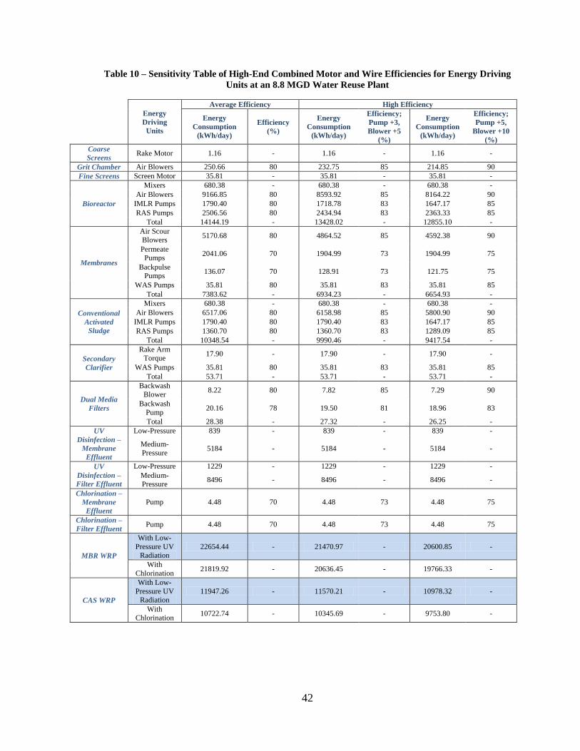
42
Table 10 – Sensitivity Table of High-End Combined Motor and Wire Efficiencies for Energy Driving
Units at an 8.8 MGD Water Reuse Plant
Energy
Driving
Units
Average Efficiency High Efficiency
Energy
Consumption
(kWh/day)
Efficiency
(%)
Energy
Consumption
(kWh/day)
Efficiency;
Pump +3,
Blower +5
(%)
Energy
Consumption
(kWh/day)
Efficiency;
Pump +5,
Blower +10
(%)
Coarse
Screens Rake Motor 1.16 - 1.16 - 1.16 -
Grit Chamber Air Blowers 250.66 80 232.75 85 214.85 90
Fine Screens Screen Motor 35.81 - 35.81 - 35.81 -
Bioreactor
Mixers 680.38 - 680.38 - 680.38 -
Air Blowers 9166.85 80 8593.92 85 8164.22 90
IMLR Pumps 1790.40 80 1718.78 83 1647.17 85
RAS Pumps 2506.56 80 2434.94 83 2363.33 85
Total 14144.19 - 13428.02 - 12855.10 -
Membranes
Air Scour
Blowers 5170.68 80 4864.52 85 4592.38 90
Permeate
Pumps 2041.06 70 1904.99 73 1904.99 75
Backpulse
Pumps 136.07 70 128.91 73 121.75 75
WAS Pumps 35.81 80 35.81 83 35.81 85
Total 7383.62 - 6934.23 - 6654.93 -
Conventional
Activated
Sludge
Mixers 680.38 - 680.38 - 680.38 -
Air Blowers 6517.06 80 6158.98 85 5800.90 90
IMLR Pumps 1790.40 80 1790.40 83 1647.17 85
RAS Pumps 1360.70 80 1360.70 83 1289.09 85
Total 10348.54 - 9990.46 - 9417.54 -
Secondary
Clarifier
Rake Arm
Torque 17.90 - 17.90 - 17.90 -
WAS Pumps 35.81 80 35.81 83 35.81 85
Total 53.71 - 53.71 - 53.71 -
Dual Media
Filters
Backwash
Blower 8.22 80 7.82 85 7.29 90
Backwash
Pump 20.16 78 19.50 81 18.96 83
Total 28.38 - 27.32 - 26.25 -
UV
Disinfection –
Membrane
Effluent
Low-Pressure 839 - 839 - 839 -
Medium-
Pressure 5184 - 5184 - 5184 -
UV
Disinfection –
Filter Effluent
Low-Pressure 1229 - 1229 - 1229 -
Medium-
Pressure 8496 - 8496 - 8496 -
Chlorination –
Membrane
Effluent
Pump 4.48 70 4.48 73 4.48 75
Chlorination –
Filter Effluent Pump 4.48 70 4.48 73 4.48 75
MBR WRP
With Low-
Pressure UV
Radiation
22654.44 - 21470.97 - 20600.85 -
With
Chlorination 21819.92 - 20636.45 - 19766.33 -
CAS WRP
With Low-
Pressure UV
Radiation
11947.26 - 11570.21 - 10978.32 -
With
Chlorination 10722.74 - 10345.69 - 9753.80 -

43
Figure 6 aides in visualizing the breakdown of the percentage of energy
consumption corresponding to each unit process of the 8.8 MGD WRPs found in this
research. It should be noted that RAS pump energy is included in the Bioreactor/CAS
energy, not the Membranes/Secondary Clarifier energy. The percentages for each unit
process inside the CAS WRP correlates to percentages calculated using WEF (2010b)
values. For instance using WEF (2010b) values, at 8.8 MGD the aerated grit chamber at
a CAS facility uses 122.72 kWh/day and a total plant energy consumption of 10,113.66
kWh/day; resulting in the aerated grit chamber using 1.21% of the total plant’s energy
consumption. This is comparable to the 1.84% at a CAS WRP found in this research.
WEF (2010b) breaks down the energy consumption for each unit process per flow,
therefore comparisons can be made with this research. However, comparisons with
individual unit processes with EPRI (2002) is not possible because the report provides
energy consumption of only the entire facility per flow.
Figure 6 – Percentage of Total Energy Consumption of the Plant per Unit Process: (a) Energy
Consumption of 8.8 MGD MBR WRP; and (b) Energy Consumption of 8.8 MGD CAS WRP
44
4. Conclusion and Discussion
This research explored the energy consumption of conventional and advanced
treatment processes used in reuse wastewater treatment inside satellite WRPs. Both
conventional and advanced unit processes were chosen to provide the same treatment
level so comparisons were equivalent. For conventional treatment with flowrates varying
from 1 to 11 MGD, a CAS process with phosphorous and nitrogen removal averaged an
energy footprint of 1382.7 kWh/MG. For advanced treatment, a MBR process with
phosphorous and nitrogen removal averaged and energy footprint of 2643.3 kWh/MG.
This demonstrates that MBR WRPs are 1.91 times more energy intensive than CAS
WRPs, costing an additional $126.06/MG treated at an average energy rate of $0.10/kWh
or 1260.6 kWh/MG. The higher cost of MBR systems is associated with air scouring of
the membranes for cleaning, which consumes an average of 23.4% of the facility’s total
energy. In addition higher cost is also related to the higher blower requirements inside
the bioreactor, as a result of a lower oxygen transfer efficiency associated with the high
solids concentrations. Disinfection of reuse plant effluent using UV radiation was shown
to be on average 100 times more energy intensive than chlorination. UV radiation was
shown to have an increase of 38.6% in the consumption of energy for disinfection of
filter effluent versus membrane effluent with low-pressure lamps, and 63.0% with
medium-pressure. Based on these results, energy savings could be realized by: using
chlorination as the disinfectant for membrane effluent, if land area permits, as MPN and
TSS levels are already minimal; and UV disinfection with low-pressure lamps would still
be advisable for filter effluent because higher concentration of microorganisms and TSS
is observed. However, if chlorination were used for filter effluent, a 2.8 times increase in

45
sodium hypochlorite per day will be expected, compared to disinfection of membrane
effluent.
The results of this study clearly show that advanced treatment processes, typically
used in reuse facilities, have a significantly larger energy footprint compared to that of
conventional processes. However, there are tradeoffs if conventional treatment processes
were to be selected over advanced treatment processes to save energy. For example, if
CAS was selected versus a MBR process a doubling in aeration volume and
corresponding land area would be needed. Furthermore, more land would be needed for
clarifiers and dual media filters to achieve comparable effluent quality. In addition,
capital costs of material (e.g. concrete) to provide for additional conventional treatment
units also need to be taken into consideration and compared to capital costs of the
advanced treatment units (e.g. membranes and UV systems). Chlorination used in place
of UV disinfection requires area for a chlorine contact basin and for chemical storage.
Therefore overall, advanced treatment processes greatly reduce the real estate area
needed but greatly increases the energy consumption of the facility.
The term ‘energy hog’ has been used for satellite WRPs to describe their high
energy consumption. This research shows if satellite WRPs are designed using
conventional treatment technologies their energy consumption is comparable to that of
non-satellite WWTPs. However, when advanced treatment technologies are
implemented in satellite WRPs, especially MBRs, ‘energy hog’ can be an adequate term.
As of late, large improvements have been made at MBR facilities in energy consumption
with the scheduling of air scour timings but more improvement is still needed. With the
ever growing increase in satellite WRPs, evaluations on the consumption of energy in

46
these facilities need to be a part of the design process. In this matter, pros and cons of the
increase in energy consumption associated with advanced treatment technologies can be
evaluated to determine which treatment processes are more suitable for the facility.
47
CHAPTER 3
IMPACTS OF ON-SITE RENEWABLE ENERGY GENERATION ON TOTAL
ENERGY CONSUMPTION AND GREENHOUSE GAS EMISSIONS OF
SATELLITE WATER REUSE PLANTS
1. Introduction
In recent decades, smaller decentralized wastewater treatment plants (WWTP),
termed satellite water reuse plants (WRP), have become very prevalent. WRPs are
satellite treatment facilities that treat wastewater from a specific part of community and
reuse the effluent in or around the location where the wastewater was collected. Due to
the close proximity and/or potential direct contact of reclaimed water with the general
public, regulations and effluent standards for reuse water are strict and are becoming
stricter (Crook, 2011). To achieve these stricter standards on effluent quality and smaller
land footprint (i.e. real estate area), additional treatment processes along with advanced
technologies are needed (Bennett, 2007; EPRI, 2002; Brandt, et al., 2011; Urkiaga, et al.,
2008). Despite the obvious benefits of water reuse and recycle, the application of
advanced treatments technologies in WRPs coupled with stringent effluent discharge
standards greater energy consumption is likely to result.
Wastewater treatment is a very energy intensive process; over recent years ways
to curb this large consumption of energy has been pursued. Energy can be curbed within
an existing WWTP by increase of efficiencies in plant equipment and the optimization of
plant processes and equipment. To achieve this reduction in energy a WWTP can
undergo a benchmarking evaluation, where energy usage for the whole plant and
48
individual processes can be computed and compared to published values (WEF, 2010b).
Another way to implement energy saving measures is with the use of supervisory control
and data acquisition (SCADA) systems. With a SCADA system, a plant can monitor
their own facility’s operational data and obtain useful energy measuring units (e.g. kW,
kWh, kWh/gal, kWh/ft3, etc.) (WEF, 2010b). However, in order to perform such an
evaluation, the necessary sensors must be installed in the plant for the unit operations of
interest. For example, plants may choose to monitor air flowrate use in the plant and the
respective energy use associated with the motors that fuel the air blowers for varying
wastewater flowrates entering the plant. With this type of analysis, it has been found that
pumping can represent up to 30% of energy consumption for wastewater treatment and
80% for clean water (Brandt, et al., 2011). To help curb this consumption the use of
modern variable speed drives in pumps can result in 83% of energy savings (Brandt, et al.,
2011). This is due to the included power factor management on these pumps, but this
does require a 4 - 5% increase in rated motor power to control the variable speed (Brandt,
et al., 2011). To assist the management of pump efficiency in WWTPs, effective
screening must be maintained because grit, rags, debris, and other solids can contribute to
higher wear rate (Brandt, et al., 2011). SCADA system energy analyses have shown that
aeration typically represents 50 to 60% of the total energy consumption in WWTPs,
however with a variety of measures, including checking control set-points, check rates
with metered electrical input, equipment performance optimization, and overall routine
maintenance, savings in energy can be up to 40% (Brandt, et al., 2011).
A ranking of energy consumption for treatment units has been developed in
wastewater treatment. In order of low energy consumption to high: biological filters;
49
anaerobic membrane bioreactor; bio-aerated flooded filter; step fed activated sludge;
nutrient removal activated sludge; and conventional membrane bioreactor (Brandt, et al.,
2011). Potential savings in energy consumption in any WWTP will be system-specific
and requires a site-specific analysis (Daigger, 2009). There is however a limit to how
much energy use within an existing plant can be curbed, because current design requires
a minimum amount of energy to run installed processes and equipment. As a result, new
approaches are needed to curb (minimize) energy consumption, not only for existing
WWTPs but also for future planned plants.
Fossil fuels, oil, coal, and gas, currently are providing over two-thirds of the
world’s energy (Demirbas, 2009). At this consumption, known petroleum reserves are
projected to be depleted in less than 50 years (Demirbas, 2009; Gude, et al., 2010). With
the world’s energy growth rate of 2% a year and the resulting energy consumption
doubling by the year 2035 relative to 1998 and tripling by 2055 (Demirbas, 2009), this
depletion rate will only get worse. Thus, the use of these fuels produces enormous
amounts of greenhouse gas (GHG) emissions, which are subsequently resulting in crucial
environmental problems worldwide including acid rain and global warming (Gude, et al.,
2010). To help maintain the reduction in GHG emissions protocols such as the Kyoto
Protocol have been adopted by the United Nations Framework Convention on Climate
Change. Kyoto Protocol was adopted by countries to help reduce GHG emissions by an
average of 5%, against 1990 levels, over a period of five years, 2008 – 2012 (UNFCCC,
2012). But since levels of GHG emissions had increased by 25% since 1990 (The World
Bank, 2010); the protocol has only had a slight effect on emissions. Even though the
50
protocol did not prove to be as successful as planned it contributes to the beginning of
change.
In the United States, 2 - 4 % of the total energy consumed is for the collection,
distribution, and treatment of wastewater and drinking water (McMahon, et al., 2011;
Daigger, 2009; U.S. EPA, 2010; Metcalf & Eddy, Inc, 2003; EPRI, 2002; WEF, 2010b).
In all WWTPs, consumption of electric power accounts for about 90% of the total energy
consumption in a plant (Mizuta, et al., 2010). This current usage of energy translated to
75 billion kWh in 1996 (U.S. EPA, 2008; U.S. EPA, 2010) and was estimated to increase
to 100 - 123.45 billion kWh in 2010 (U.S. EPA, 2010; EPRI, 2009). This consumption
emits roughly 116 billion lbs (52 million metric tonnes) of carbon dioxide (CO2) into the
atmosphere (McMahon, et al., 2011; NRDC, 2009). In order to decrease this production
of GHG emissions and dependency on fossil fuels, the use of renewable energy in
wastewater treatment has become popular in replacing grid connect as a supply for
energy. In addition, efforts have been spent towards wastewater treatment generating
some of the energy they consumed via methane generation from anaerobic sludge
digestion and the installation of photovoltaic (PV) solar panels throughout or around the
plant (Palmer, 2009; Seeta, et al., 2011).
Anaerobic sludge digestion, is generally not found in satellite WRPs, due to the
lack of solids handling at the facility to achieve a smaller real estate area. However,
introduction of membrane bioreactors (MBR) into satellite reuse plants is expected to
significantly reduce land acreage needed. Therefore, application of anaerobic digesters at
these facilities should now be re-evaluated. With the increase of pretreatment
requirements before the use of a MBR, solids screening removal has become more
51
stringent; thus a richer thicker primary sludge is obtained that can be processed directly in
a digester without the need for thickening. For this reason, only one additional unit
process is needed to have an energy producing unit at the facility, the digester itself.
In using digesters at a WRP, only primary (screened) sludge can be selected to be
diverted to the digester to allow for more energy production and less energy consumption.
This is because if even a small amount of waste activated sludge (WAS) were to be
blended into the process, the rate of biological reaction in the digester would decrease
(Metcalf & Eddy, Inc, 2003). With the WAS being directly discharged back into the
collection trunk without processing through the digester, the volume and the overall
acreage of the digester will be smaller. Using a single-stage high-rate mesophilic
anaerobic digester also provides a small acreage for the digester. With the digestion of
the primary sludge, odors can be greatly reduced when compared to discharging
undigested primary sludge back into the collection system for further processing.
The use of renewable energy in industry as a whole has had a slow start.
Renewable energy only represents a 14-16% total of the world’s energy (Demirbas, 2009;
Gude, et al., 2010). This number has been projected to reach 48-50% by the year 2040
(Demirbas, 2009; Gude, et al., 2010). This projection has been paralleled with the recent
growth rate in renewable energy application such as wind and solar energy during 2009 -
2010 (Trabish, 2012). With the development of new technology, renewable energy has
become more cost effective, comparable to grid connect using fossil fuels. Renewable
energies, geothermal, solar, and wind, cost 0.07, 0.05-0.09, and 0.05/kWh, respectively;
while grid connected electricity costs 0.05-0.09/kWh (Gude, et al., 2010). With the cost
of fossil fuels rapidly rising (Mizuta, et al., 2010; Brandt, et al., 2011), the need to
52
conserve energy and transition from fossil fuels to renewable energy has now become a
necessity over a luxury.
The use of advanced treatment technologies to treat reuse water requires a large
increase in energy consumption compared to conventional unit processes (Chapter 2). In
the past, energy consumption and GHG generation has not been a concern in WWTP
design and especially in reuse plant design. However, the current efforts to minimize
GHG emissions and related energy footprint challenges the actual benefits of reuse plants
with advanced treatment. Previous work has been done on the energy consumption in
satellite WRPs and was found that with advanced treatment technologies, such as a MBR,
requires on average a 1.67 increase in energy consumption compared to a conventional
activated sludge system (CAS) (Chapter 2). However, a complete evaluation on GHG
emissions and the renewable energy potential of a WRP have not been investigated to
date. In this research, a WRP was evaluated to determine the GHG emissions associated
with conventional and advanced treatment units. In addition, the renewable energy
potential inside the plant was investigated based on acreage available from basin and
membrane/clarifier area for a PV solar system, and from biosolids digestion from fine
screened (primary) sludge.
2. Methodology
The flow diagram for the WRP considered in this study is presented in Figure 7.
In order of treatment, the unit processes include: coarse screen, aerated grit chambers,
fine screen, conventional activated sludge (CAS) system, membranes, and UV
disinfection. When comparing conventional versus advanced unit processes, the

53
membranes were replaced by the combination of secondary clarification and dual media
filtration, and UV disinfection by chlorination.

54
Figure 7 – Process Flow Diagram of the Water Reuse Plant for Which Greenhouse Gas Emissions
are Evaluated
Fig
ure
7 –
Pro
cess
Flo
w D
iag
ram
of
the
Wa
ter
Reu
se P
lan
t fo
r W
hic
h G
reen
ho
use
Ga
s E
mis
sio
ns
are
Eva
lua
ted

55
2.1 Influent and Effluent Quality
The influent characteristics and effluent requirements for the WRP are presented
in Table 11. The requirements are typical water reuse standards found in California and
Florida, with the exception for the need to remove nutrients. A five-stage modified
Bardenpho CAS system is provided at the facility for the removal of the nutrients
phosphorous and nitrogen (WEF, 2012; WEF, 2011).
Table 11 – Plant Influent and Effluent Process Characteristics Found in the Water Reuse Plant
Parameter Influent
Characteristics
Effluent
Requirements
BOD (mg/L) 250 30
TSS (mg/L) 309 30
TKN (mg/L as N) 42 –
NH3 (mg/L as N) 34 0.5
TN (mg/L as N) – 10
TP (mg/L as P) 8 0.2
TC (MPN/100 mL) – 2.2
TC, daily max (MPN/100 mL) – 23
Minimum Temp (°C) 18.3 18.3
2.2 Energy Consumption in Unit Processes of the Water Reuse Plant
To determine the energy consumption associated with the reuse plant, the energy
driving unit from each process was identified and the energy associated with it was
computed (computations shown in Chapter 2). These computations were done using
typical design equations available in reference literature (Metcalf & Eddy, Inc, 2003;
WEF, 2010a; Qasim, 1999; Davis, 2010; Lin, 2007; WEF, 2012). Energy consumption
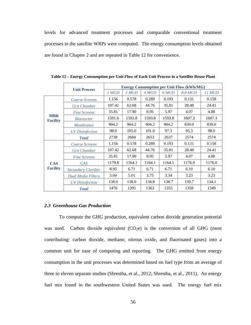
56
levels for advanced treatment processes and comparable conventional treatment
processes in the satellite WRPs were computed. The energy consumption levels obtained
are found in Chapter 2 and are repeated in Table 12 for convenience.
Table 12 – Energy Consumption per Unit Flow of Each Unit Process in a Satellite Reuse Plant
Unit Process
Energy Consumption per Unit Flow (kWh/MG)
1 MGD 2 MGD 4 MGD 6 MGD 8.8 MGD 11 MGD
MBR
Facility
Coarse Screens 1.156 0.578 0.289 0.193 0.131 0.158
Grit Chamber 107.42 62.68 44.76 35.81 28.48 24.41
Fine Screens 35.81 17.90 8.95 5.97 4.07 4.88
Bioreactor 1591.6 1593.8 1593.8 1593.8 1607.3 1607.3
Membranes 904.2 904.2 904.2 904.2 839.0 839.0
UV Disinfection 98.0 105.0 101.0 97.3 95.3 98.0
Total 2738 2684 2653 2637 2574 2574
CAS
Facility
Coarse Screens 1.156 0.578 0.289 0.193 0.131 0.158
Grit Chamber 107.42 62.68 44.76 35.81 28.48 24.41
Fine Screens 35.81 17.90 8.95 5.97 4.07 4.88
CAS 1179.8 1164.1 1164.1 1164.1 1176.0 1176.0
Secondary Clarifier 8.95 6.71 6.71 6.71 6.10 6.10
Dual Media Filters 5.04 5.01 3.75 3.34 3.23 3.23
UV Disinfection 138.0 138.0 134.8 138.7 139.7 134.1
Total 1476 1395 1363 1355 1358 1349
2.3 Greenhouse Gas Production
To compute the GHG production, equivalent carbon dioxide generation potential
was used. Carbon dioxide equivalent (CO2e) is the conversion of all GHG (most
contributing: carbon dioxide, methane, nitrous oxide, and fluorinated gases) into a
common unit for ease of computing and reporting. The GHG emitted from energy
consumption in the unit processes was determined based on fuel type from an average of
three to eleven separate studies (Shrestha, et al., 2012; Shrestha, et al., 2011). An energy
fuel mix found in the southwestern United States was used. The energy fuel mix
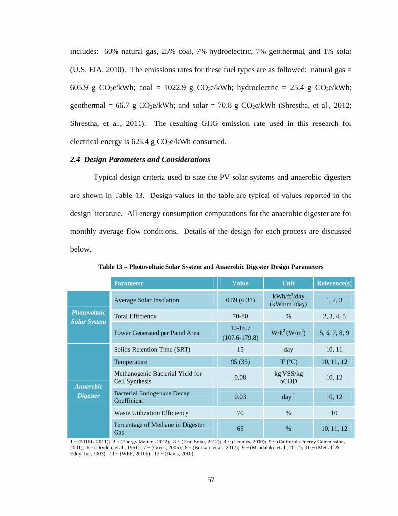
57
includes: 60% natural gas, 25% coal, 7% hydroelectric, 7% geothermal, and 1% solar
(U.S. EIA, 2010). The emissions rates for these fuel types are as followed: natural gas =
605.9 g CO2e/kWh; coal = 1022.9 g CO2e/kWh; hydroelectric = 25.4 g CO2e/kWh;
geothermal = 66.7 g CO2e/kWh; and solar = 70.8 g CO2e/kWh (Shrestha, et al., 2012;
Shrestha, et al., 2011). The resulting GHG emission rate used in this research for
electrical energy is 626.4 g CO2e/kWh consumed.
2.4 Design Parameters and Considerations
Typical design criteria used to size the PV solar systems and anaerobic digesters
are shown in Table 13. Design values in the table are typical of values reported in the
design literature. All energy consumption computations for the anaerobic digester are for
monthly average flow conditions. Details of the design for each process are discussed
below.
Table 13 – Photovoltaic Solar System and Anaerobic Digester Design Parameters
Parameter Value Unit Reference(s)
Photovoltaic
Solar System
Average Solar Insolation 0.59 (6.31) kWh/ft2/day
(kWh/m2/day) 1, 2, 3
Total Efficiency 70-80 % 2, 3, 4, 5
Power Generated per Panel Area 10-16.7
(107.6-179.8) W/ft2
(W/m2) 5, 6, 7, 8, 9
Anaerobic
Digester
Solids Retention Time (SRT) 15 day 10, 11
Temperature 95 (35) ºF (ºC) 10, 11, 12
Methanogenic Bacterial Yield for
Cell Synthesis 0.08
kg VSS/kg
bCOD 10, 12
Bacterial Endogenous Decay
Coefficient 0.03 day-1 10, 12
Waste Utilization Efficiency 70 % 10
Percentage of Methane in Digester
Gas 65 % 10, 11, 12
1 ~ (NREL, 2011); 2 ~ (Energy Matters, 2012); 3 ~ (Find Solar, 2012); 4 ~ (Leonics, 2009); 5 ~ (California Energy Commission,
2001); 6 ~ (Dryden, et al., 1961); 7 ~ (Green, 2005); 8 ~ (Burkart, et al., 2012); 9 ~ (Mandalaki, et al., 2012); 10 ~ (Metcalf &
Eddy, Inc, 2003); 11 ~ (WEF, 2010b); 12 ~ (Davis, 2010)
58
2.4.1 Anaerobic Digester
Key parameters used in the design of the single-stage high-rate mesophilic
anaerobic digester can be found in Table 13. The HRT, equivalent to the SRT, was used
in the determination of the volume required for the digester (Metcalf & Eddy, Inc, 2003).
The amount of methane-forming volatile solids synthesized per day was determined
using the complete-mix high-rate digester equation, followed by the calculation of the
volume of methane gas using kinetic equations (Metcalf & Eddy, Inc, 2003; Davis, 2010).
These were done taking into account the volume of methane gas at the operating
temperature of 35ºC. An egg-shaped digester was used in the design to provide a higher
mixing efficiency, improved homogeneous biomass, and most importantly, a smaller real
estate area in the WRP (Metcalf & Eddy, Inc, 2003; WEF, 2010b).
The anaerobic digestion process produces methane gas that can be used for energy
generation; however, digestion itself consumes energy. Energy consumption for the
anaerobic digester is driven by the mixers providing a homogeneous biomass mixture and
by the heat-exchanger providing heating for the sludge and heat losses through the
digester walls. Mixer energy requirements were determined based on the volume of the
digester, using an average energy consumption of 6.5 W/m3 (WEF, 2010b). The energy
requirement to heat the sludge was determined using (Metcalf & Eddy, Inc, 2003; Davis,
2010; WEF, 2010b):
iss TTCMq (1)
where q = heat required, J/day; Ms = mass flow of sludge, kg/day; Cs = specific heat of
sludge, J/kg∙ºC; T = digestion temperature, ºC; and Ti = influent sludge temperature, ºC.
For purposes of this research, 4200 J/kg∙ºC was used for the specific heat of sludge
59
(Metcalf & Eddy, Inc, 2003). The energy required to compensate for the loss of heat
through the walls of the digester were determined as (Metcalf & Eddy, Inc, 2003; Davis,
2010; WEF, 2010b):
TUAq (2)
where q = heat loss, J/sec; U = overall coefficient of heat transfer, J/m2∙sec∙ºC; A =
cross-sectional area perpendicular to heat flow, m2; and ΔT = change in temperature
between digestion and surface in question. Coefficients of heat transfer used in the
research are 0.68, 0.85, and 0.91 W/m2∙ºC for the walls, floor, and roof, respectively
(Metcalf & Eddy, Inc, 2003; Davis, 2010; WEF, 2010b). Energy production from the
combustion of digester gas was determined using:
HVeE (3)
where E = energy generated, kJ/day; H = heat of combustion, kJ/m3; V = volume of gas
produced per day, m3/day; and e = electrical efficiency. In this research, 37,000 kJ/m
3
was used for the heat of combustion of methane (WEF, 2010b). An electrical efficiency
of 33% was used based off the efficiency for an internal combustion engine (ICE) (WEF,
2010b).
2.4.2 Photovoltaic Solar System
Parameters used in the design of the PV solar system can be found in Table 13.
Real estate area available for the PV system was determined based off basin and
membrane/clarifier area in the form of a shaded structure with tilt single-axis panels. The
system size was determined by multiplying the available area by the amount of power
that can be generated per solar area. In this research, a radiative efficiency (i.e. panel
60
efficiency) of 15% was used, which provides 13.9 W of power generated per square foot
of solar paneling. The energy production from this system size was calculated using:
pss IeIPE / (4)
Where E = energy generated, kWh/day; Ps = PV system size, kW; Is = solar insolation,
kWh/m2/day; e = combined efficiency; and Ip = panel irradiance, kW/m
2. The combined
efficiency takes into account manufacture rating, wiring and power point tracking losses,
and the inverter efficiency (Energy Matters, 2012; California Energy Commission, 2001).
A combined efficiency of 80% was used. A panel irradiance of 1000 W/m2 was used for
the PV systems per ASTM G173-03 (ASTM International, 2012).
A sensitivity analysis was performed on solar panel efficiency. If a low radiative
efficiency of 10.8% (10 W/ft2) were used (California Energy Commission, 2001; Dryden,
et al., 1961), this would be a reduction of 28.2% of the energy generated by the panels. If
a high radiative efficiency of 18% (16.7 W/ft2) were used (Green, 2005), an increase in
energy generation of 20.0% would result.
3. Results and Analysis
Estimated energy consumption of the major energy driving and producing units
for the anaerobic digester and PV solar system for varying flowrates in the WRP are
presented in Table 14. Overall net totals of the energy consumption and generation are
also provided.
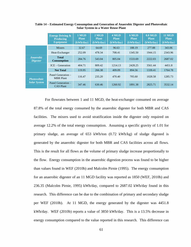
61
Table 14 – Estimated Energy Consumption and Generation of Anaerobic Digester and Photovoltaic
Solar System in a Water Reuse Plant
Energy Driving &
Producing
Equipment
1 MGD
Plant
(kWh/day)
2 MGD
Plant
(kWh/day)
4 MGD
Plant
(kWh/day)
6 MGD
Plant
(kWh/day)
8.8 MGD
Plant
(kWh/day)
11 MGD
Plant
(kWh/day)
Anaerobic
Digester
Mixers 32.67 64.69 96.63 188.19 277.88 343.06
Heat-Exchanger 252.09 478.34 708.41 1345.50 1944.15 2343.96
Total
Consumption 284.76 543.04 805.04 1533.69 2222.03 2687.02
ICE – Generation 404.71 809.42 1214.13 2428.25 3561.44 4451.8
Net Total 119.95 266.38 409.09 894.56 1339.41 1764.78
Photovoltaic
Solar System
Panel Generation –
MBR Plant 116.47 235.20 470.40 705.60 1028.58 1285.73
Panel Generation –
CAS Plant 347.46 630.46 1260.92 1891.38 2825.71 3532.14
For flowrates between 1 and 11 MGD, the heat-exchanger consumed on average
87.8% of the total energy consumed by the anaerobic digester for both MBR and CAS
facilities. The mixers used to avoid stratification inside the digester only required on
average 12.2% of the total energy consumption. Assuming a specific gravity of 1.01 for
primary sludge, an average of 653 kWh/ton (0.72 kWh/kg) of sludge digested is
generated by the anaerobic digester for both MBR and CAS facilities across all flows.
This is the result for all flows as the volume of primary sludge increase proportionally to
the flow. Energy consumption in the anaerobic digestion process was found to be higher
than values found in WEF (2010b) and Malcolm Pirnie (1995). The energy consumption
for an anaerobic digester of an 11 MGD facility was reported as 1850 (WEF, 2010b) and
236.35 (Malcolm Pirnie, 1995) kWh/day, compared to 2687.02 kWh/day found in this
research. This difference can be due to the combination of primary and secondary sludge
per WEF (2010b). At 11 MGD, the energy generated by the digester was 4451.8
kWh/day. WEF (2010b) reports a value of 3850 kWh/day. This is a 13.5% decrease in
energy consumption compared to the value reported in this research. This difference can
62
be due to the type of energy generator used, as different generators have different
efficiencies. If microturbines with an efficiency of 27% were used, the energy generated
would be 3642.4 kWh/day, making a difference of only 5.4% less comparing to WEF
(2010b). In addition, a pattern is seen in the anaerobic digester, as flow increases the
fraction of energy generated over energy consumed by the digester increases by an
average of 3.1% across all flows.
For flowrates between 1 and 11 MGD, energy generation of the PV solar system
in CAS facilities was proven to be on average 2.75 times higher than MBR facilities due
to the large real estate size. The real estate size is directly proportional to the amount of
energy generated as CAS facilities were on average 2.75 higher in real estate area
compared to MBR facilities. The real estate sizes and their corresponding PV system
sizes can be found in Table 15. For both MBR and CAS facilities, 0.07 kWh/day is
generated per square foot of solar paneling. Future improvements in PV solar cell
performance will only make this energy generation even greater. Since 1954, PV solar
cells have increased from a two percent radiative efficiency to percentages of twenty-five
plus in laboratory settings (Green, 2005; Spanggaard, et al., 2004; Green, 2012; Hecht,
2010). This is compared to the average 15% radiative efficiency (13.9 W/ft2) used in this
research.
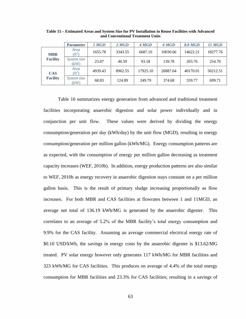
63
Table 15 – Estimated Areas and System Size for PV Installation in Reuse Facilities with Advanced
and Conventional Treatment Units
Parameter 1 MGD 2 MGD 4 MGD 6 MGD 8.8 MGD 11 MGD
MBR
Facility
Area
(ft2) 1655.78 3343.55 6687.10 10030.66 14622.21 18277.76
System size
(kW) 23.07 46.59 93.18 139.78 203.76 254.70
CAS
Facility
Area
(ft2) 4939.43 8962.55 17925.10 26887.64 40170.01 50212.51
System size
(kW) 68.83 124.89 249.79 374.68 559.77 699.71
Table 16 summarizes energy generation from advanced and traditional treatment
facilities incorporating anaerobic digestion and solar power individually and in
conjunction per unit flow. These values were derived by dividing the energy
consumption/generation per day (kWh/day) by the unit flow (MGD), resulting in energy
consumption/generation per million gallon (kWh/MG). Energy consumption patterns are
as expected, with the consumption of energy per million gallon decreasing as treatment
capacity increases (WEF, 2010b). In addition, energy production patterns are also similar
to WEF, 2010b as energy recovery in anaerobic digestion stays constant on a per million
gallon basis. This is the result of primary sludge increasing proportionally as flow
increases. For both MBR and CAS facilities at flowrates between 1 and 11MGD, an
average net total of 136.19 kWh/MG is generated by the anaerobic digester. This
correlates to an average of 5.2% of the MBR facility’s total energy consumption and
9.9% for the CAS facility. Assuming an average commercial electrical energy rate of
$0.10 USD/kWh, the savings in energy costs by the anaerobic digester is $13.62/MG
treated. PV solar energy however only generates 117 kWh/MG for MBR facilities and
323 kWh/MG for CAS facilities. This produces on average of 4.4% of the total energy
consumption for MBR facilities and 23.3% for CAS facilities; resulting in a savings of
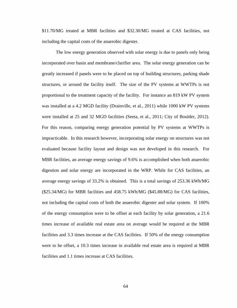
64
$11.70/MG treated at MBR facilities and $32.30/MG treated at CAS facilities, not
including the capital costs of the anaerobic digester.
The low energy generation observed with solar energy is due to panels only being
incorporated over basin and membrane/clarifier area. The solar energy generation can be
greatly increased if panels were to be placed on top of building structures, parking shade
structures, or around the facility itself. The size of the PV systems at WWTPs is not
proportional to the treatment capacity of the facility. For instance an 819 kW PV system
was installed at a 4.2 MGD facility (Drainville, et al., 2011) while 1000 kW PV systems
were installed at 25 and 32 MGD facilities (Seeta, et al., 2011; City of Boulder, 2012).
For this reason, comparing energy generation potential by PV systems at WWTPs is
impracticable. In this research however, incorporating solar energy on structures was not
evaluated because facility layout and design was not developed in this research. For
MBR facilities, an average energy savings of 9.6% is accomplished when both anaerobic
digestion and solar energy are incorporated in the WRP. While for CAS facilities, an
average energy savings of 33.2% is obtained. This is a total savings of 253.36 kWh/MG
($25.34/MG) for MBR facilities and 458.75 kWh/MG ($45.88/MG) for CAS facilities,
not including the capital costs of both the anaerobic digester and solar system. If 100%
of the energy consumption were to be offset at each facility by solar generation, a 21.6
times increase of available real estate area on average would be required at the MBR
facilities and 3.3 times increase at the CAS facilities. If 50% of the energy consumption
were to be offset, a 10.3 times increase in available real estate area is required at MBR
facilities and 1.1 times increase at CAS facilities.
65
Table 16 – Energy Consumption and Generation per Unit Flow of the Anaerobic Digester and
Photovoltaic Solar System
Unit Process
Energy Consumption per Unit Flow (kWh/MG)
1 MGD 2 MGD 4 MGD 6 MGD 8.8 MGD 11 MGD
MBR
Facility
Wastewater
Treatment Total 2738 2684 2653 2637 2574 2574
Anaerobic Digester 284.8 271.5 201.3 255.6 252.5 244.3
Anaerobic Digester
Generation 405 405 304 405 405 405
Net Total w/Digester 2618 2551 2551 2488 2422 2413
Photovoltaic
System Generation 116 118 118 118 117 117
Net Total w/PV 2622 2567 2535 2520 2457 2457
Net Total w/Digester
and PV 2502 2433 2433 2371 2305 2296
CAS
Facility
Wastewater
Treatment Total 1476 1395 1363 1355 1358 1349
Anaerobic Digester 284.8 271.5 201.3 255.6 252.5 244.3
Anaerobic Digester
Generation 405 405 304 405 405 405
Net Total w/Digester 1356 1262 1261 1206 1206 1188
Photovoltaic
System Generation 347 315 315 315 321 321
Net Total w/PV 1129 1080 1048 1040 1037 1028
Net Total w/Digester
and PV 1009 947 946 890 884 867
The costs for both anaerobic digesters and PV solar systems are only for
operational energy consumption. Capital costs to install PV systems and digesters were
evaluated based off current literature, but were not extensively explored. For PV solar
systems, ranges vary widely based on the size and type of system, from $1.99 - $7.40/W
generated (Barbose, et al., 2011; Goodrich, et al., 2012). In this research an average
value of $4.00/W was assumed. A wide range in capital costs was also found for
anaerobic digesters, from $2574 - $7000/kWh generated (Navaratnasamy, et al., 2008;
IRENA, 2012). An average value of $5,000/kWh was assumed in this research. Table
17 shows the payback period in years for both energy generating systems. A low,
medium, and high energy price as well as municipality and/or government incentives are
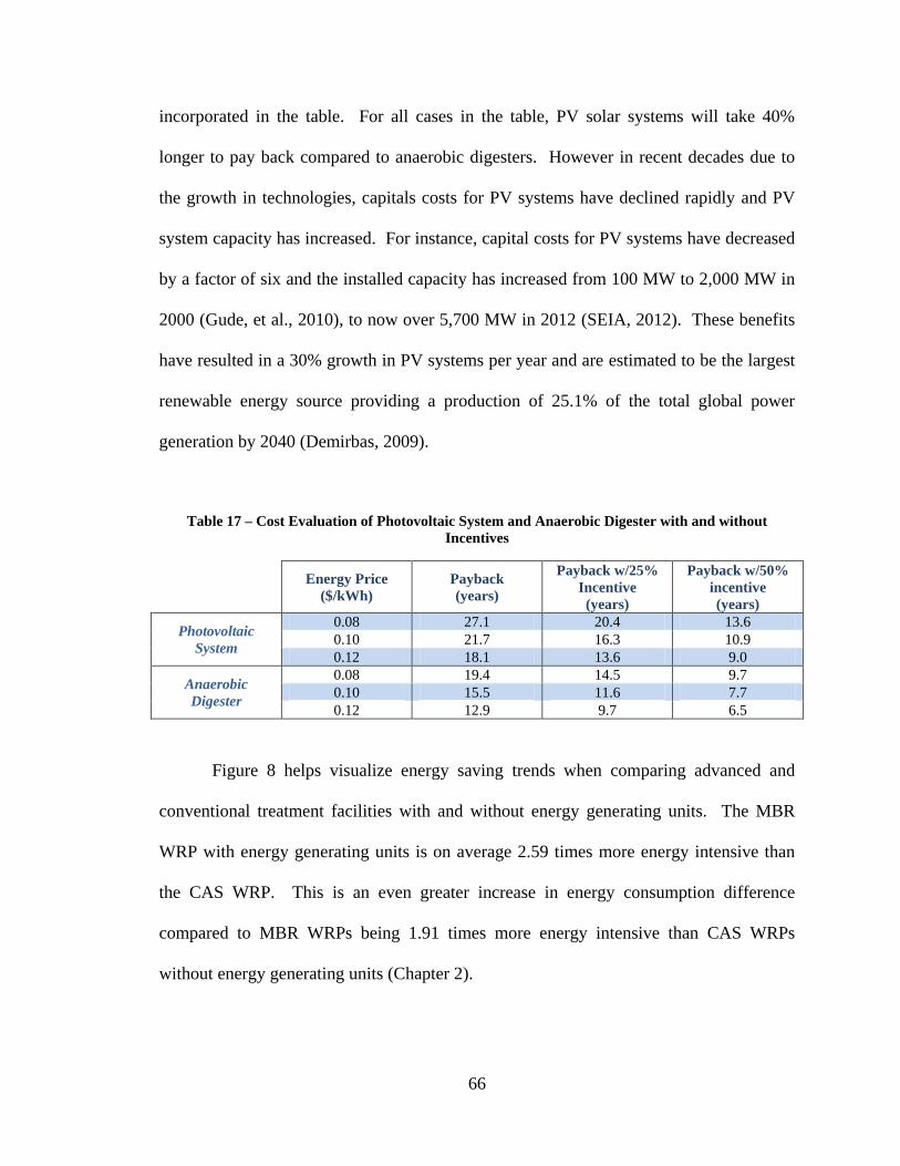
66
incorporated in the table. For all cases in the table, PV solar systems will take 40%
longer to pay back compared to anaerobic digesters. However in recent decades due to
the growth in technologies, capitals costs for PV systems have declined rapidly and PV
system capacity has increased. For instance, capital costs for PV systems have decreased
by a factor of six and the installed capacity has increased from 100 MW to 2,000 MW in
2000 (Gude, et al., 2010), to now over 5,700 MW in 2012 (SEIA, 2012). These benefits
have resulted in a 30% growth in PV systems per year and are estimated to be the largest
renewable energy source providing a production of 25.1% of the total global power
generation by 2040 (Demirbas, 2009).
Table 17 – Cost Evaluation of Photovoltaic System and Anaerobic Digester with and without
Incentives
Energy Price
($/kWh)
Payback
(years)
Payback w/25%
Incentive
(years)
Payback w/50%
incentive
(years)
Photovoltaic
System
0.08 27.1 20.4 13.6
0.10 21.7 16.3 10.9
0.12 18.1 13.6 9.0
Anaerobic
Digester
0.08 19.4 14.5 9.7
0.10 15.5 11.6 7.7
0.12 12.9 9.7 6.5
Figure 8 helps visualize energy saving trends when comparing advanced and
conventional treatment facilities with and without energy generating units. The MBR
WRP with energy generating units is on average 2.59 times more energy intensive than
the CAS WRP. This is an even greater increase in energy consumption difference
compared to MBR WRPs being 1.91 times more energy intensive than CAS WRPs
without energy generating units (Chapter 2).
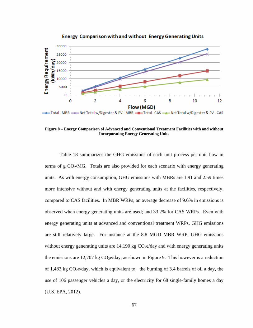
67
Figure 8 – Energy Comparison of Advanced and Conventional Treatment Facilities with and without
Incorporating Energy Generating Units
Table 18 summarizes the GHG emissions of each unit process per unit flow in
terms of g CO2/MG. Totals are also provided for each scenario with energy generating
units. As with energy consumption, GHG emissions with MBRs are 1.91 and 2.59 times
more intensive without and with energy generating units at the facilities, respectively,
compared to CAS facilities. In MBR WRPs, an average decrease of 9.6% in emissions is
observed when energy generating units are used; and 33.2% for CAS WRPs. Even with
energy generating units at advanced and conventional treatment WRPs, GHG emissions
are still relatively large. For instance at the 8.8 MGD MBR WRP, GHG emissions
without energy generating units are 14,190 kg CO2e/day and with energy generating units
the emissions are 12,707 kg CO2e/day, as shown in Figure 9. This however is a reduction
of 1,483 kg CO2e/day, which is equivalent to: the burning of 3.4 barrels of oil a day, the
use of 106 passenger vehicles a day, or the electricity for 68 single-family homes a day
(U.S. EPA, 2012).
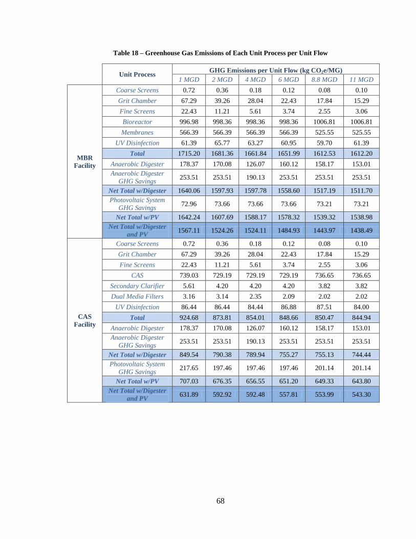
68
Table 18 – Greenhouse Gas Emissions of Each Unit Process per Unit Flow
Unit Process
GHG Emissions per Unit Flow (kg CO2e/MG)
1 MGD 2 MGD 4 MGD 6 MGD 8.8 MGD 11 MGD
MBR
Facility
Coarse Screens 0.72 0.36 0.18 0.12 0.08 0.10
Grit Chamber 67.29 39.26 28.04 22.43 17.84 15.29
Fine Screens 22.43 11.21 5.61 3.74 2.55 3.06
Bioreactor 996.98 998.36 998.36 998.36 1006.81 1006.81
Membranes 566.39 566.39 566.39 566.39 525.55 525.55
UV Disinfection 61.39 65.77 63.27 60.95 59.70 61.39
Total 1715.20 1681.36 1661.84 1651.99 1612.53 1612.20
Anaerobic Digester 178.37 170.08 126.07 160.12 158.17 153.01
Anaerobic Digester
GHG Savings 253.51 253.51 190.13 253.51 253.51 253.51
Net Total w/Digester 1640.06 1597.93 1597.78 1558.60 1517.19 1511.70
Photovoltaic System
GHG Savings 72.96 73.66 73.66 73.66 73.21 73.21
Net Total w/PV 1642.24 1607.69 1588.17 1578.32 1539.32 1538.98
Net Total w/Digester
and PV 1567.11 1524.26 1524.11 1484.93 1443.97 1438.49
CAS
Facility
Coarse Screens 0.72 0.36 0.18 0.12 0.08 0.10
Grit Chamber 67.29 39.26 28.04 22.43 17.84 15.29
Fine Screens 22.43 11.21 5.61 3.74 2.55 3.06
CAS 739.03 729.19 729.19 729.19 736.65 736.65
Secondary Clarifier 5.61 4.20 4.20 4.20 3.82 3.82
Dual Media Filters 3.16 3.14 2.35 2.09 2.02 2.02
UV Disinfection 86.44 86.44 84.44 86.88 87.51 84.00
Total 924.68 873.81 854.01 848.66 850.47 844.94
Anaerobic Digester 178.37 170.08 126.07 160.12 158.17 153.01
Anaerobic Digester
GHG Savings 253.51 253.51 190.13 253.51 253.51 253.51
Net Total w/Digester 849.54 790.38 789.94 755.27 755.13 744.44
Photovoltaic System
GHG Savings 217.65 197.46 197.46 197.46 201.14 201.14
Net Total w/PV 707.03 676.35 656.55 651.20 649.33 643.80
Net Total w/Digester
and PV 631.89 592.92 592.48 557.81 553.99 543.30

69
Figure 9 – Greenhouse Gas Emissions due to Electrical Energy Consumption with and without
Energy Generating Units at 8.8 MGD
4. Conclusion and Discussion
This research explored the renewable energy generation potential of a satellite
WRP with the addition of a PV solar system and anaerobic digestion. This was
performed for two types of facilities: conventional (CAS bioreactor with secondary
clarifiers and dual media filtration) and advanced (bioreactor with membrane filtration)
treatment satellite WRPs. In addition, the associated GHG emissions for both
conventional and advanced treatment processes were evaluated. For conventional
treatment, it was found that 9.9% and 23.3% of the facility’s total energy consumption
can be generated by anaerobic digestion and solar energy, respectively. For advanced
treatment, 5.2% and 4.4% of the facility’s total energy consumption can be generated by
anaerobic digestion and solar energy, respectively. It was observed that energy recovery
generation for both anaerobic digestion and PV systems is constant on a per million
70
gallon basis. When both energy generating units are incorporated in satellite WRPs, an
average energy savings of 33.2% is accomplished in a CAS facility and 9.6% in a MBR
facility, resulting in MBR WRPs averaging 1.86 times more energy intensive than CAS
WRPs. This translates to a cost savings in electricity of $25.34/MG treated for MBR
facilities and $45.88/MG treated at CAS facilities using an average commercial energy
rate of $0.10/kWh. The payback periods for both anaerobic digestion and solar energy
were investigated and it was found that no matter the energy rate or the incentive, solar
energy requires on average 40% longer to pay back compared to anaerobic digestion.
Furthermore, the results of this research showed that in terms of GHG emissions,
MBR WRPs without energy generating units are 1.91 times more intensive than CAS
WRPs and 2.59 times more intensive with energy generating units. With or without
energy generating units, GHG emissions are still very large at WRPs. For MBR WRPs,
1,656 kg CO2e/MG treated is emitted without energy generating units at the facilities,
while 1,497 kg CO2e/MG treated is emitted at the facilities with energy generating units.
For CAS WRPs, 866 kg CO2e/MG treated is emitted at facilities without energy
generating units, while 579 kg CO2e/MG treated is emitted at facilities with energy
generating units. This research has shown that with the addition of energy generating
units the energy consumption of the facility can have the potential to be greatly decreased.
Performing such energy analyses will provide a means for engineers and operators in the
decision making process regarding sustainability of using advanced or conventional
treatment technologies at a reuse facility. The term ‘energy hog’ is often used for
satellite WRPs. With time, as more energy saving and producing measures are

71
implemented, satellite WRPs will have the prospective to be termed ‘energy neutral’
facilities, in replacement of ‘energy hog’.
72
CHAPTER 4
CONCLUSIONS
Wastewater treatment is a very energy intensive process and with the continued
increase in satellite water reuse plants (WRPs), and the associated advanced treatment
processes with these plants, this energy consumption will only increase. In the arid
southwestern United States where nutrient requirements must be met, along with the
strict standards and regulations on reuse water, increased energy consumption is
inevitable. This research investigated the intertwined resources of wastewater and energy,
along with the associated greenhouse gas (GHG) emissions from the treatment of
wastewater at satellite WRPs. With the growing concerns of GHG emissions and linked
crucial environmental problems, implementation of renewable energy resources was used
to minimize these emissions. Objectives of this research were: (1) to investigate the
impact of conventional and advanced treatment technologies on energy consumption at
satellite WRPs; (2) to evaluate the impact of renewable technologies implementation on
energy consumption and associated GHG generation at satellite WRPs; and (3) to
compare energy footprint and associated real estate area required for advanced and
conventional treatment technologies. The conclusions of this research are as follows:
When comparing advanced treatment processes, membrane bioreactor (MBR),
with conventional treatment processes, conventional activated sludge (CAS) with
secondary clarifiers and dual media filters, the MBR requires on average 2.10
times more energy to treat to the same effluent quality for flowrates between 1
and 11 MGD.

73
Comparing advanced disinfection, ultraviolet (UV) radiation, with conventional
disinfection, chlorination, resulted in UV disinfection being 100 times more
energy intensive for both MBR and CAS WRPs. When comparing the energy
consumption of disinfecting membrane effluent against filter effluent with UV
disinfection, it was found that an increase of 38.6% in energy is required to treat
filter effluent with low-pressure lamps, and 63.0% with medium-pressure.
Comparing energy consumption with low-pressure lamps versus medium-pressure
lamps, it was found that medium-pressure lamps required an increase of 5.96 and
7.01 times in energy consumption for MBR and CAS WRPs, respectively. When
disinfecting with chlorination, CAS WRPs require 2.8 times the amount of
sodium hypochlorite needed compared to MBR WRPs.
For flowrates between 1 to 11 MGD, MBR and CAS WRPs with low-pressure
UV disinfection required on average 2643.3 and 1382.7 kWh/MG, respectively.
This demonstrates the MBR WRPs are 1.91 times more energy intensive than
CAS WRPs, costing and additional $126.06/MG treated in energy consumption
using an average commercial energy rate of $0.10/kWh.
The highest energy consuming unit in the MBR WRP contributing to the large
energy footprint is the air scour blowers; requiring on average 23.7% of the
facility’s total energy consumption.
A sensitivity analysis on ‘wire-to-water’ efficiencies has shown that even with a
slight increase or decrease in efficiencies (±5% for pumps and ±10% for blowers),
the total energy consumption of the entire plant can be greatly affected, by as
much as an 11.3% increase or 9.4% decrease.

74
Comparing basin real estate area between the MBR and CAS WRPs, it was found
that the CAS WRPs required a doubling in aeration volume, resulting in a
doubling in the acreage. Total real estate area (the addition of secondary
treatment and filtration units) for MBR WRPs was on average 1666 ft2/MG, while
CAS WRPs was 4585 ft2/MG. Comparing total real estate yields an increase of
2.75 times in acreage for CAS WRPs. This means it costs MBR WRPs an
increase in energy consumption of 0.43 kWh/MG per square foot of real estate
saved or $21.50/MG per 500 ft2 of real estate saved.
Using the real estate area for photovoltaic (PV) solar systems, 4.4% of the
facility’s total energy consumption can be generated for MBR WRPs and 23.3%
can be generated for CAS WRPs.
If anaerobic digesters were to be added to a plant’s unit processes for energy
generation by primary sludge digestion, 5.2 and 9.9% of the total facility’s energy
consumption can be generated for MBR and CAS WRPs, respectively.
When both PV solar systems and anaerobic digesters are incorporated at a WRP,
savings in energy can be 9.6 and 33.2% of the total facilities energy consumption
for MBR and CAS WRPs, respectively. This translates to a cost savings in
electricity of $25.34/MG treated for MBR facilities and $45.88/MG treated at
CAS facilities.
With or without the use of energy generating units, GHG emissions due to
electrical energy consumption are still very large at WRPs. Considering an
energy fuel mix of 60% natural gas, 25% coal, 7% hydroelectric, 7% geothermal,
and 1% solar, emissions for MBR WRPs are 1,656 kg CO2e/MG treated without
75
energy generating units at the facilities, while 1,497 kg CO2e/MG treated is
emitted at the facilities with energy generating units. This is a reduction of 9.6%.
For CAS WRPs, 866 kg CO2e/MG treated is emitted at facilities without energy
generating units, while 579 kg CO2e/MG treated is emitted at facilities with
energy generating units. Achieving a 33.2% reduction.
This research has shown that with the use of design criteria and equations for unit
processes, along with their associated fundamental energy equations, engineers can
determine a very accurate estimate of energy consumption for individual unit processes
of an entire WRP. The values found closely match actual energy consumption reported
by varies literature. This approach highlights a means for engineers and operators to
target unit processes that are candidates for reduction in energy consumption and provide
a basis for decision making regarding sustainability of using advanced treatment
technologies at a reuse facility. In addition, with the increase in satellite WRPs and the
overall increase in advanced treatment technologies at wastewater treatment plants in
general, evaluations on the consumption of energy at these facilities needs to be a part of
the design process; providing pros and cons to determine the need for certain unit process
and the overall sustainability of the facility.
This research has provided a beginning in the determination of energy
consumption and the corresponding GHG emissions inside satellite WRPs. Both
advanced and conventional treatment processes commonly used at these facilities have
been evaluated in this study. Two forms of renewable energy generation were also
evaluated to determine the energy savings and GHG reduction that can be achieved at
76
these facilities. However, this study is not comprehensive and much work remains to be
performed. Below are suggestions for future research:
To investigate the impact on energy consumption for different advanced and
conventional treatment processes other than the ones investigated in this research.
Investigate the potential energy generation for other renewable technologies.
To design and evaluate a total facility layout for which actual drawings are
available. In this matter a complete facility energy calculation can be done as
pumping stations will now be included (e.g. influent pumping station, primary
effluent pumping station, and filter influent pumping station).
To evaluate renewable energy implementation in facilities for which actual
drawings are available. This will provide a total acreage of the facility giving the
ability to increase solar area to the tops of structures (e.g. rooftops and parking
structures).
To perform equipment energy audits as equipment ages to determine if energy
consumption of the reuse facility increases with age.
To perform life cycle analysis to compare GHG emissions of various unit
processes.
To evaluate total GHG emissions from WRPs, this includes emissions from the
unit processes themselves (e.g. carbon dioxide, methane, and nitrous oxide from
biological treatment with activated sludge).
77
APPENDIX A
DESIGN PARAMETERS AND EQUATIONS FOR UNIT OPERATIONS AND
ENERGY COMPUTATION EQUATIONS USED
A-1 Coarse Screens
The initial open channel leading into the coarse screens was designed using Manning’s
equation:
2/13/2 SARn
KQ n (Sturm, 2010; Mays, 2010)
where Q = flow rate; Kn = 1.0 with R in m and Q in m3/s, and 1.49 for R in ft and Q in
ft3/s; n = Manning’s coefficient; R = hydraulic radius; and S = bed slope. For purposes
of this research, a value of 0.015 (Sturm, 2010; Mays, 2010) was used for the Manning’s
coefficient in determination of channel properties. Velocity in this channel should
exceed 1.3 ft/sec (0.4 m/s) during minimum flows to ensure grit deposition is avoided
(WEF, 2010a). If this is impossible due to diurnal flows, a velocity of 3 ft/sec (0.9 m/s)
should be used during peak flows to ensure resuspension of solids (WEF, 2010a). The
maximum approach velocity was in the desired range at 2.35 ft/sec (Metcalf & Eddy, Inc,
2003; Qasim, 1999; WEF, 2010a). Key parameters used in the design can be found in
Table A 1.
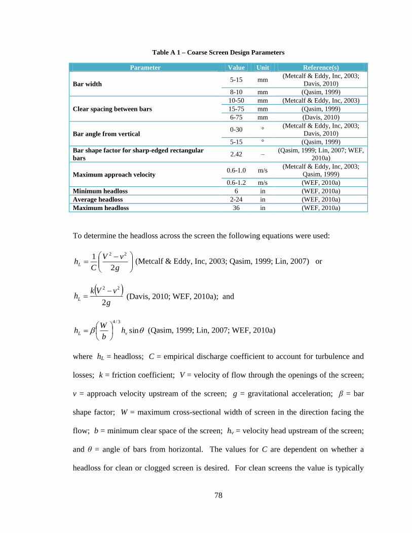
78
Table A 1 – Coarse Screen Design Parameters
Parameter Value Unit Reference(s)
Bar width 5-15 mm
(Metcalf & Eddy, Inc, 2003;
Davis, 2010)
8-10 mm (Qasim, 1999)
Clear spacing between bars
10-50 mm (Metcalf & Eddy, Inc, 2003)
15-75 mm (Qasim, 1999)
6-75 mm (Davis, 2010)
Bar angle from vertical 0-30 °
(Metcalf & Eddy, Inc, 2003;
Davis, 2010)
5-15 ° (Qasim, 1999)
Bar shape factor for sharp-edged rectangular
bars 2.42 –
(Qasim, 1999; Lin, 2007; WEF,
2010a)
Maximum approach velocity 0.6-1.0 m/s
(Metcalf & Eddy, Inc, 2003;
Qasim, 1999)
0.6-1.2 m/s (WEF, 2010a)
Minimum headloss 6 in (WEF, 2010a)
Average headloss 2-24 in (WEF, 2010a)
Maximum headloss 36 in (WEF, 2010a)
To determine the headloss across the screen the following equations were used:
g
vV
ChL
2
1 22
(Metcalf & Eddy, Inc, 2003; Qasim, 1999; Lin, 2007) or
g
vVkhL
2
22 (Davis, 2010; WEF, 2010a); and
sin
3/4
vL hb
Wh
(Qasim, 1999; Lin, 2007; WEF, 2010a)
where hL = headloss; C = empirical discharge coefficient to account for turbulence and
losses; k = friction coefficient; V = velocity of flow through the openings of the screen;
v = approach velocity upstream of the screen; g = gravitational acceleration; β = bar
shape factor; W = maximum cross-sectional width of screen in the direction facing the
flow; b = minimum clear space of the screen; hv = velocity head upstream of the screen;
and θ = angle of bars from horizontal. The values for C are dependent on whether a
headloss for clean or clogged screen is desired. For clean screens the value is typically
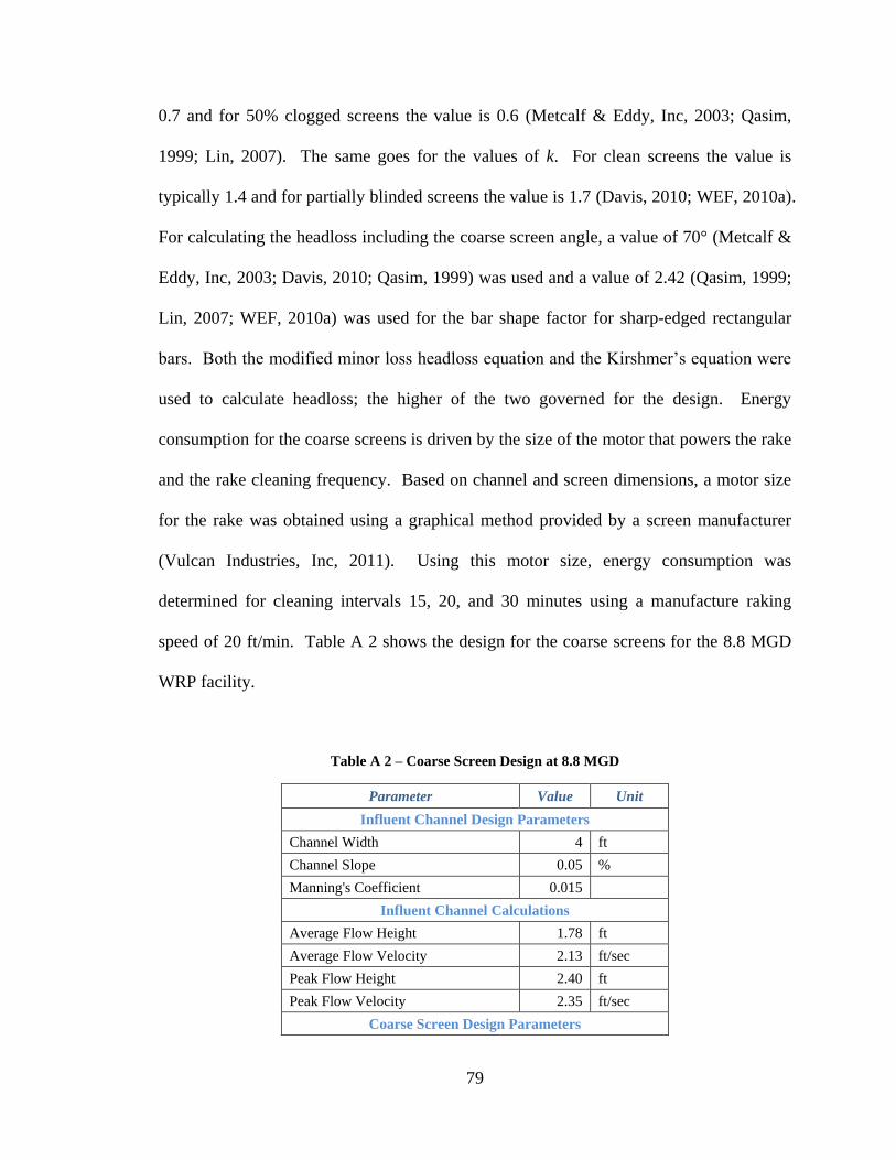
79
0.7 and for 50% clogged screens the value is 0.6 (Metcalf & Eddy, Inc, 2003; Qasim,
1999; Lin, 2007). The same goes for the values of k. For clean screens the value is
typically 1.4 and for partially blinded screens the value is 1.7 (Davis, 2010; WEF, 2010a).
For calculating the headloss including the coarse screen angle, a value of 70° (Metcalf &
Eddy, Inc, 2003; Davis, 2010; Qasim, 1999) was used and a value of 2.42 (Qasim, 1999;
Lin, 2007; WEF, 2010a) was used for the bar shape factor for sharp-edged rectangular
bars. Both the modified minor loss headloss equation and the Kirshmer’s equation were
used to calculate headloss; the higher of the two governed for the design. Energy
consumption for the coarse screens is driven by the size of the motor that powers the rake
and the rake cleaning frequency. Based on channel and screen dimensions, a motor size
for the rake was obtained using a graphical method provided by a screen manufacturer
(Vulcan Industries, Inc, 2011). Using this motor size, energy consumption was
determined for cleaning intervals 15, 20, and 30 minutes using a manufacture raking
speed of 20 ft/min. Table A 2 shows the design for the coarse screens for the 8.8 MGD
WRP facility.
Table A 2 – Coarse Screen Design at 8.8 MGD
Parameter Value Unit
Influent Channel Design Parameters
Channel Width 4 ft
Channel Slope 0.05 %
Manning's Coefficient 0.015
Influent Channel Calculations
Average Flow Height 1.78 ft
Average Flow Velocity 2.13 ft/sec
Peak Flow Height 2.40 ft
Peak Flow Velocity 2.35 ft/sec
Coarse Screen Design Parameters
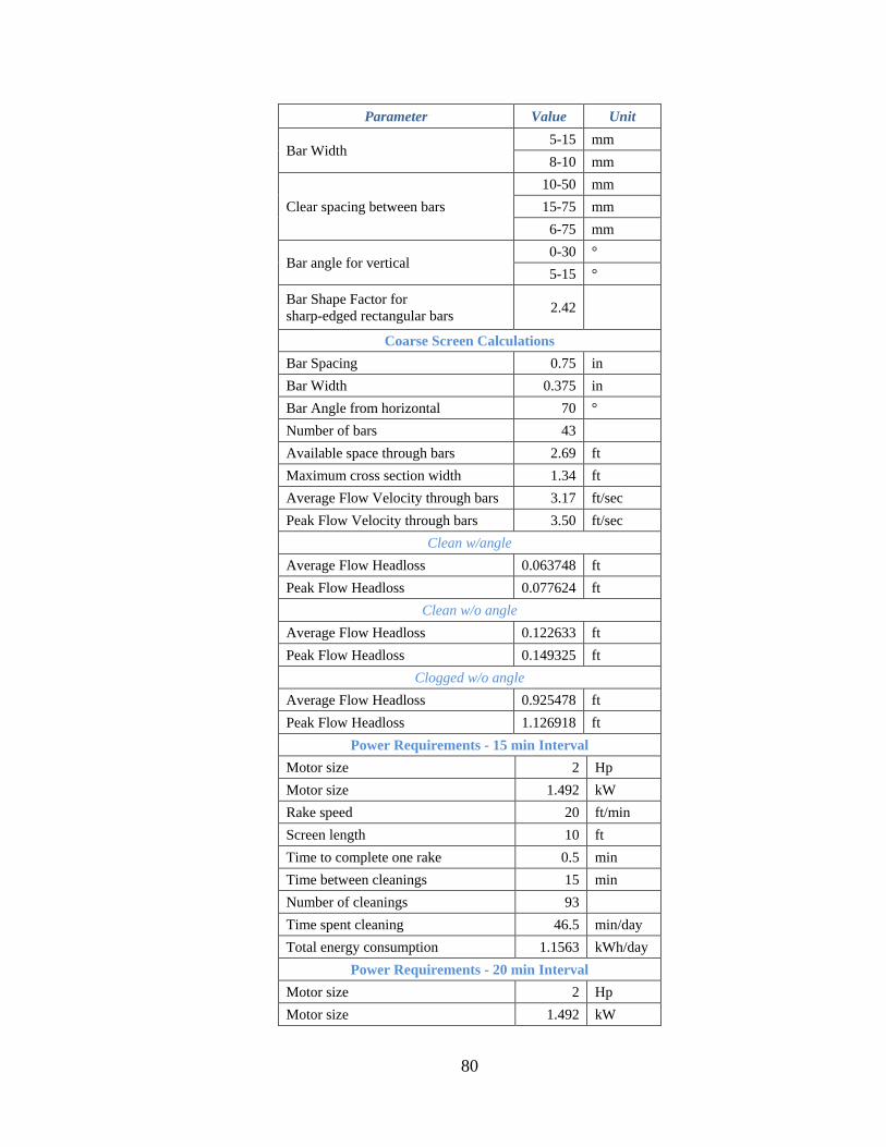
80
Parameter Value Unit
Bar Width 5-15 mm
8-10 mm
Clear spacing between bars
10-50 mm
15-75 mm
6-75 mm
Bar angle for vertical 0-30 °
5-15 °
Bar Shape Factor for
sharp-edged rectangular bars 2.42
Coarse Screen Calculations
Bar Spacing 0.75 in
Bar Width 0.375 in
Bar Angle from horizontal 70 °
Number of bars 43
Available space through bars 2.69 ft
Maximum cross section width 1.34 ft
Average Flow Velocity through bars 3.17 ft/sec
Peak Flow Velocity through bars 3.50 ft/sec
Clean w/angle
Average Flow Headloss 0.063748 ft
Peak Flow Headloss 0.077624 ft
Clean w/o angle
Average Flow Headloss 0.122633 ft
Peak Flow Headloss 0.149325 ft
Clogged w/o angle
Average Flow Headloss 0.925478 ft
Peak Flow Headloss 1.126918 ft
Power Requirements - 15 min Interval
Motor size 2 Hp
Motor size 1.492 kW
Rake speed 20 ft/min
Screen length 10 ft
Time to complete one rake 0.5 min
Time between cleanings 15 min
Number of cleanings 93
Time spent cleaning 46.5 min/day
Total energy consumption 1.1563 kWh/day
Power Requirements - 20 min Interval
Motor size 2 Hp
Motor size 1.492 kW
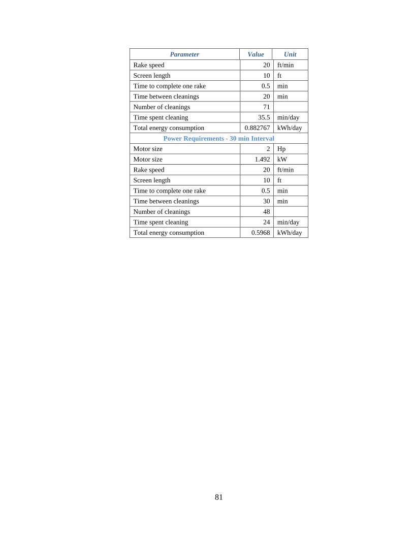
81
Parameter Value Unit
Rake speed 20 ft/min
Screen length 10 ft
Time to complete one rake 0.5 min
Time between cleanings 20 min
Number of cleanings 71
Time spent cleaning 35.5 min/day
Total energy consumption 0.882767 kWh/day
Power Requirements - 30 min Interval
Motor size 2 Hp
Motor size 1.492 kW
Rake speed 20 ft/min
Screen length 10 ft
Time to complete one rake 0.5 min
Time between cleanings 30 min
Number of cleanings 48
Time spent cleaning 24 min/day
Total energy consumption 0.5968 kWh/day
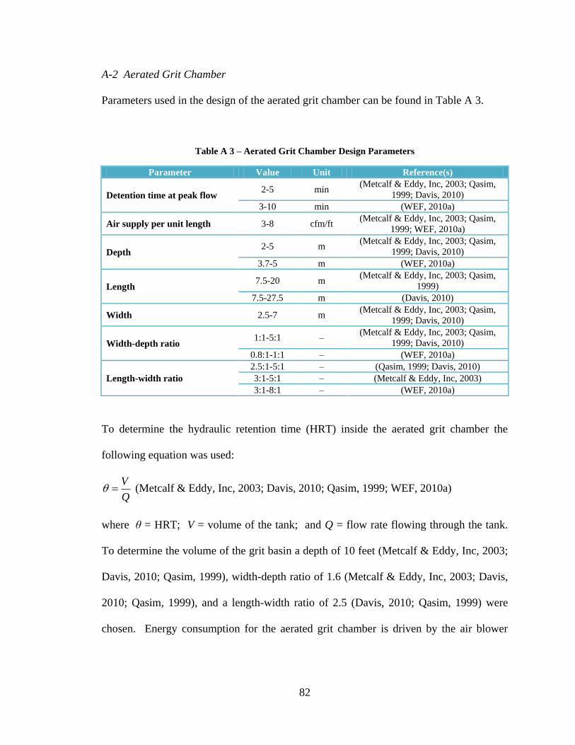
82
A-2 Aerated Grit Chamber
Parameters used in the design of the aerated grit chamber can be found in Table A 3.
Table A 3 – Aerated Grit Chamber Design Parameters
Parameter Value Unit Reference(s)
Detention time at peak flow 2-5 min
(Metcalf & Eddy, Inc, 2003; Qasim,
1999; Davis, 2010)
3-10 min (WEF, 2010a)
Air supply per unit length 3-8 cfm/ft (Metcalf & Eddy, Inc, 2003; Qasim,
1999; WEF, 2010a)
Depth 2-5 m
(Metcalf & Eddy, Inc, 2003; Qasim,
1999; Davis, 2010)
3.7-5 m (WEF, 2010a)
Length 7.5-20 m
(Metcalf & Eddy, Inc, 2003; Qasim,
1999)
7.5-27.5 m (Davis, 2010)
Width 2.5-7 m (Metcalf & Eddy, Inc, 2003; Qasim,
1999; Davis, 2010)
Width-depth ratio 1:1-5:1 –
(Metcalf & Eddy, Inc, 2003; Qasim,
1999; Davis, 2010)
0.8:1-1:1 – (WEF, 2010a)
Length-width ratio
2.5:1-5:1 – (Qasim, 1999; Davis, 2010)
3:1-5:1 – (Metcalf & Eddy, Inc, 2003)
3:1-8:1 – (WEF, 2010a)
To determine the hydraulic retention time (HRT) inside the aerated grit chamber the
following equation was used:
Q
V (Metcalf & Eddy, Inc, 2003; Davis, 2010; Qasim, 1999; WEF, 2010a)
where θ = HRT; V = volume of the tank; and Q = flow rate flowing through the tank.
To determine the volume of the grit basin a depth of 10 feet (Metcalf & Eddy, Inc, 2003;
Davis, 2010; Qasim, 1999), width-depth ratio of 1.6 (Metcalf & Eddy, Inc, 2003; Davis,
2010; Qasim, 1999), and a length-width ratio of 2.5 (Davis, 2010; Qasim, 1999) were
chosen. Energy consumption for the aerated grit chamber is driven by the air blower

83
capacity used to maintain discrete particle sedimentation and can be estimated by the
following equation:
1/*/428.4283.0 bdas PPeTqEBHP
(U.S. EPA, 1989)
where BHP = brake horsepower, hp; qs = required flow rate, scfm; Ta = blower inlet air
temperature, °R; e = blower and motor combined efficiency; Pd = blower discharge
pressure, psia (the addition of atmospheric pressure and the system head); and Pb = field
atmospheric pressure, psia. System head was estimated as per (U.S. EPA, 1989) using
headloss values for diffuser (0.70 psi; 4.826 kPa), piping (0.15 psi; 1.034 kPa), and inlet
valve and filter headloss (0.30 psi; 2.068 kPa). Atmospheric pressure at 2,000 feet (609.6
meters) elevation was used and a combined blower and motor efficiency of 80% were
assumed (Metcalf & Eddy, Inc, 2003; Davis, 2010). Table A 4 shows the design for the
aerated grit chamber for the 8.8 MGD WRP facility.
Table A 4 – Aerated Grit Chamber Design at 8.8 MGD
Parameter Value Unit
Aerated Grit Chamber Design Parameters
Number of hoppers 3
Detention time at peak flow 2-5 min
3-10 min
Air supply per unit length 3-8 cfm/ft
Dimensions
Depth 2-5 m
3.7-5 m
Length 7.5-20 m
7.5-27.5 m
Width 2.5-7 m
Width-depth ratio 1:1-5:1
0.8:1-1:1
Length-width ratio 2.5:1-5:1
3:1-5:1
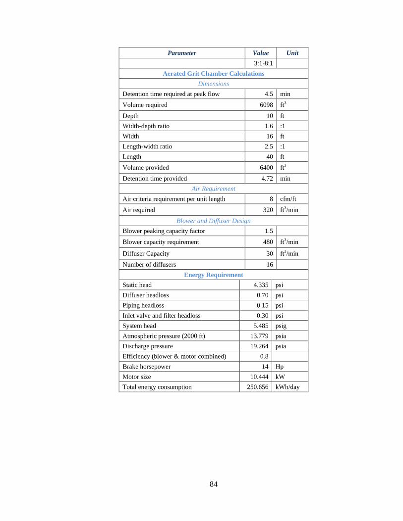
84
Parameter Value Unit
3:1-8:1
Aerated Grit Chamber Calculations
Dimensions
Detention time required at peak flow 4.5 min
Volume required 6098 ft3
Depth 10 ft
Width-depth ratio 1.6 :1
Width 16 ft
Length-width ratio 2.5 :1
Length 40 ft
Volume provided 6400 ft3
Detention time provided 4.72 min
Air Requirement
Air criteria requirement per unit length 8 cfm/ft
Air required 320 ft3/min
Blower and Diffuser Design
Blower peaking capacity factor 1.5
Blower capacity requirement 480 ft3/min
Diffuser Capacity 30 ft3/min
Number of diffusers 16
Energy Requirement
Static head 4.335 psi
Diffuser headloss 0.70 psi
Piping headloss 0.15 psi
Inlet valve and filter headloss 0.30 psi
System head 5.485 psig
Atmospheric pressure (2000 ft) 13.779 psia
Discharge pressure 19.264 psia
Efficiency (blower & motor combined) 0.8
Brake horsepower 14 Hp
Motor size 10.444 kW
Total energy consumption 250.656 kWh/day
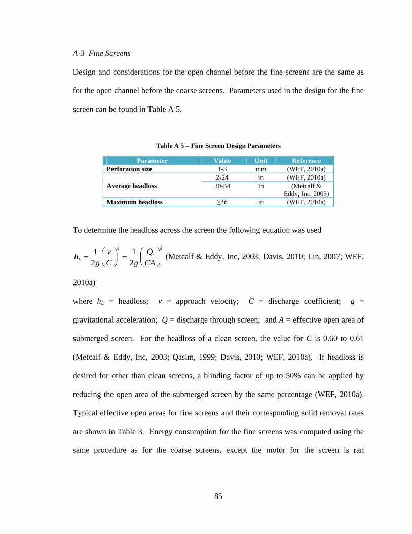
85
A-3 Fine Screens
Design and considerations for the open channel before the fine screens are the same as
for the open channel before the coarse screens. Parameters used in the design for the fine
screen can be found in Table A 5.
Table A 5 – Fine Screen Design Parameters
Parameter Value Unit Reference
Perforation size 1-3 mm (WEF, 2010a)
Average headloss
2-24 in (WEF, 2010a)
30-54 In (Metcalf &
Eddy, Inc, 2003)
Maximum headloss ≥36 in (WEF, 2010a)
To determine the headloss across the screen the following equation was used
22
2
1
2
1
CA
Q
gC
v
ghL
(Metcalf & Eddy, Inc, 2003; Davis, 2010; Lin, 2007; WEF,
2010a)
where hL = headloss; v = approach velocity; C = discharge coefficient; g =
gravitational acceleration; Q = discharge through screen; and A = effective open area of
submerged screen. For the headloss of a clean screen, the value for C is 0.60 to 0.61
(Metcalf & Eddy, Inc, 2003; Qasim, 1999; Davis, 2010; WEF, 2010a). If headloss is
desired for other than clean screens, a blinding factor of up to 50% can be applied by
reducing the open area of the submerged screen by the same percentage (WEF, 2010a).
Typical effective open areas for fine screens and their corresponding solid removal rates
are shown in Table 3. Energy consumption for the fine screens was computed using the
same procedure as for the coarse screens, except the motor for the screen is ran
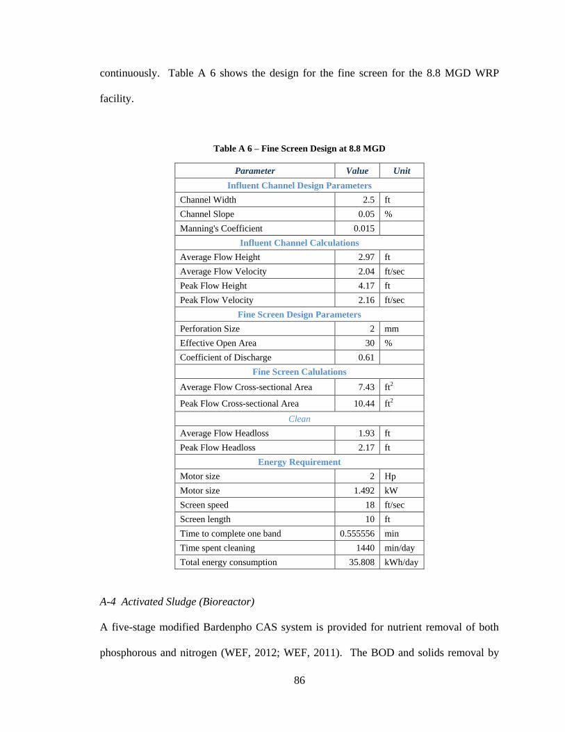
86
continuously. Table A 6 shows the design for the fine screen for the 8.8 MGD WRP
facility.
Table A 6 – Fine Screen Design at 8.8 MGD
Parameter Value Unit
Influent Channel Design Parameters
Channel Width 2.5 ft
Channel Slope 0.05 %
Manning's Coefficient 0.015
Influent Channel Calculations
Average Flow Height 2.97 ft
Average Flow Velocity 2.04 ft/sec
Peak Flow Height 4.17 ft
Peak Flow Velocity 2.16 ft/sec
Fine Screen Design Parameters
Perforation Size 2 mm
Effective Open Area 30 %
Coefficient of Discharge 0.61
Fine Screen Calulations
Average Flow Cross-sectional Area 7.43 ft2
Peak Flow Cross-sectional Area 10.44 ft2
Clean
Average Flow Headloss 1.93 ft
Peak Flow Headloss 2.17 ft
Energy Requirement
Motor size 2 Hp
Motor size 1.492 kW
Screen speed 18 ft/sec
Screen length 10 ft
Time to complete one band 0.555556 min
Time spent cleaning 1440 min/day
Total energy consumption 35.808 kWh/day
A-4 Activated Sludge (Bioreactor)
A five-stage modified Bardenpho CAS system is provided for nutrient removal of both
phosphorous and nitrogen (WEF, 2012; WEF, 2011). The BOD and solids removal by

87
the coarse and fine screens were based on data provided by manufacturers (Table 4).
Microbiological parameters of the activated sludge process can be found in Table 5. Key
design parameters for the activated sludge system are found in Table A 7 and design
equations are found in Table A 8.
Table A 7 – Activated Sludge Design Parameters
Parameter Value Unit Reference
Solids Retention Time 10 day (Menniti, et al., 2011)
Internal Mixed Liquor Recycle
(IMLR) 200 %
(WEF, 2010a; WEF,
2006; WEF, 2011)
Return Activated Sludge (RAS)
Recycle Ratio – MBR 400 %
(WEF, 2010a; WEF,
2006; WEF, 2012)
RAS Recycle Ratio – CAS 100 %
(WEF, 2010a;
Metcalf & Eddy, Inc,
2003)
VFA 43 mg/L
Table A 8 – Design Equations for Activated Sludge Process
Parameter Equation Reference
Hydraulic Retention Time
(HRT)
Q
RV
Q
Vx
10
(Rittmann, et al.,
2001)
HRT in Reactor
SS
S
SK
Xq
i
i
a
rln
ˆ
1
(Rittmann, et al.,
2001)
Solids retention time (SRT) ww
a
ee
a
ax
QXQX
VX
(Rittmann, et al.,
2001)
SRT at which
microorganisms washout
0
0
0min
ˆSS
KbbqYS
SKx
SbqY
xˆ
1lim
min
(Rittmann, et al.,
2001)
Reactor substrate
concentration 1ˆ
1
bqY
bKS
x
x
(Rittmann, et al.,
2001)
Reactor minimum substrate
concentration
x
bqY
bKS
ˆmin
(Rittmann, et al.,
2001)
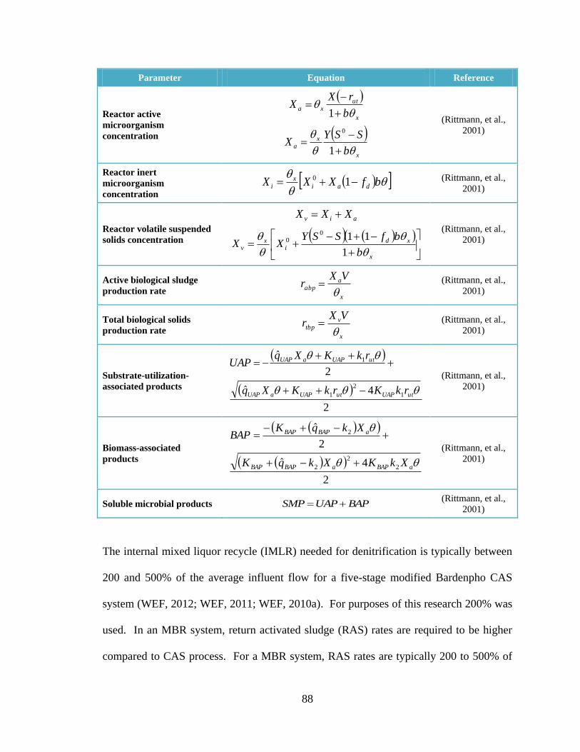
88
Parameter Equation Reference
Reactor active
microorganism
concentration
x
utxa
b
rXX
1
x
xa
b
SSYX
1
0
(Rittmann, et al.,
2001)
Reactor inert
microorganism
concentration
bfXXX dai
xi 10
(Rittmann, et al.,
2001)
Reactor volatile suspended
solids concentration
aiv XXX
x
xdi
xv
b
bfSSYXX
1
1100
(Rittmann, et al.,
2001)
Active biological sludge
production rate x
aabp
VXr
(Rittmann, et al.,
2001)
Total biological solids
production rate x
vtbp
VXr
(Rittmann, et al.,
2001)
Substrate-utilization-
associated products
2
4ˆ
2
ˆ
1
2
1
1
utUAPutUAPaUAP
utUAPaUAP
rkKrkKXq
rkKXqUAP
(Rittmann, et al.,
2001)
Biomass-associated
products
2
4ˆ
2
ˆ
2
2
2
2
aBAPaBAPBAP
aBAPBAP
XkKXkqK
XkqKBAP
(Rittmann, et al.,
2001)
Soluble microbial products BAPUAPSMP (Rittmann, et al.,
2001)
The internal mixed liquor recycle (IMLR) needed for denitrification is typically between
200 and 500% of the average influent flow for a five-stage modified Bardenpho CAS
system (WEF, 2012; WEF, 2011; WEF, 2010a). For purposes of this research 200% was
used. In an MBR system, return activated sludge (RAS) rates are required to be higher
compared to CAS process. For a MBR system, RAS rates are typically 200 to 500% of
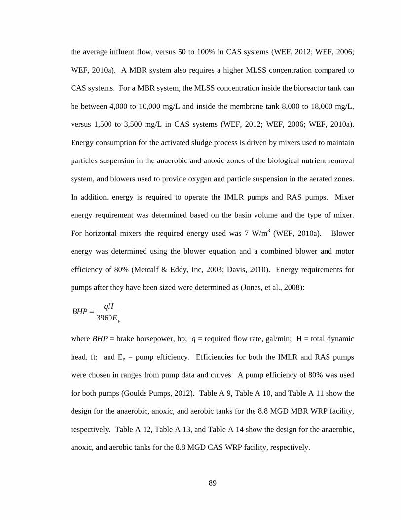
89
the average influent flow, versus 50 to 100% in CAS systems (WEF, 2012; WEF, 2006;
WEF, 2010a). A MBR system also requires a higher MLSS concentration compared to
CAS systems. For a MBR system, the MLSS concentration inside the bioreactor tank can
be between 4,000 to 10,000 mg/L and inside the membrane tank 8,000 to 18,000 mg/L,
versus 1,500 to 3,500 mg/L in CAS systems (WEF, 2012; WEF, 2006; WEF, 2010a).
Energy consumption for the activated sludge process is driven by mixers used to maintain
particles suspension in the anaerobic and anoxic zones of the biological nutrient removal
system, and blowers used to provide oxygen and particle suspension in the aerated zones.
In addition, energy is required to operate the IMLR pumps and RAS pumps. Mixer
energy requirement was determined based on the basin volume and the type of mixer.
For horizontal mixers the required energy used was 7 W/m3 (WEF, 2010a). Blower
energy was determined using the blower equation and a combined blower and motor
efficiency of 80% (Metcalf & Eddy, Inc, 2003; Davis, 2010). Energy requirements for
pumps after they have been sized were determined as (Jones, et al., 2008):
pE
qHBHP
3960
where BHP = brake horsepower, hp; q = required flow rate, gal/min; H = total dynamic
head, ft; and Ep = pump efficiency. Efficiencies for both the IMLR and RAS pumps
were chosen in ranges from pump data and curves. A pump efficiency of 80% was used
for both pumps (Goulds Pumps, 2012). Table A 9, Table A 10, and Table A 11 show the
design for the anaerobic, anoxic, and aerobic tanks for the 8.8 MGD MBR WRP facility,
respectively. Table A 12, Table A 13, and Table A 14 show the design for the anaerobic,
anoxic, and aerobic tanks for the 8.8 MGD CAS WRP facility, respectively.

90
Table A 9– Anaerobic Tank Design at 8.8 MGD for MBR WRP
Parameter Value Unit
Flow Parameters
Maximum Month 2.2 MGD
Maximum Month 3.4034 cfs
Flow Type Complete Mix Assumed
4 Trains
Tank Sizing
Length 24 ft
Width 26 ft
Depth 19.1 ft
Volume 11918.4 ft3
Influent Parameters
Assume 50% BOD Removal in Fine Screens 0.5
Assume 80% TSS Removal in Fine Screens 0.8
VFA 43 mg/L
TSS 61.8 mg/L
BOD 125 mg/L
BODL 187.5 mg/L
Acetate to COD Conversion 1.048 g COD/g Acetate
Microbiological Parameters – PAOs
K 1 mg VFA/L
Y 0.3 g VSS/g VFA
3.17 g VFA/g VSS-day
0.95 g VSS/g VSS-day
b 0.04 g VSS/g VSS-day
fd 0.8
Anaerobic Zone Design
SRT 10 days
HRT 0.041 days
HRT 58 minutes
Smin 0.044 mg VFA/L
S -1.0400 mg VFA/L
Xa Generated In An Zone 9.2049 mg VSS/L
Xi Generated In An Zone 0.0104 mg VSS/L
VFAs Remaining 0.044 mg VFA/L
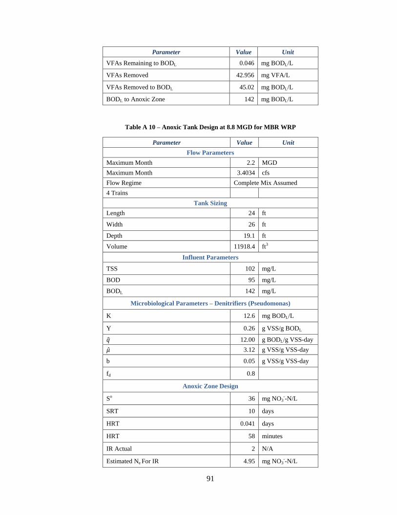
91
Parameter Value Unit
VFAs Remaining to BODL 0.046 mg BODL/L
VFAs Removed 42.956 mg VFA/L
VFAs Removed to BODL 45.02 mg BODL/L
BODL to Anoxic Zone 142 mg BODL/L
Table A 10 – Anoxic Tank Design at 8.8 MGD for MBR WRP
Parameter Value Unit
Flow Parameters
Maximum Month 2.2 MGD
Maximum Month 3.4034 cfs
Flow Regime Complete Mix Assumed
4 Trains
Tank Sizing
Length 24 ft
Width 26 ft
Depth 19.1 ft
Volume 11918.4 ft3
Influent Parameters
TSS 102 mg/L
BOD 95 mg/L
BODL 142 mg/L
Microbiological Parameters – Denitrifiers (Pseudomonas)
K 12.6 mg BODL/L
Y 0.26 g VSS/g BODL
12.00 g BODL/g VSS-day
3.12 g VSS/g VSS-day
b 0.05 g VSS/g VSS-day
fd 0.8
Anoxic Zone Design
So 36 mg NO3--N/L
SRT 10 days
HRT 0.041 days
HRT 58 minutes
IR Actual 2 N/A
Estimated Ne For IR 4.95 mg NO3--N/L
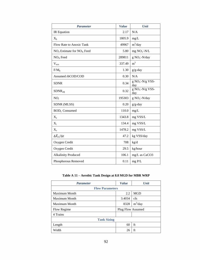
92
Parameter Value Unit
IR Equation 2.17 N/A
Xb 1805.9 mg/L
Flow Rate to Anoxic Tank 49967 m3/day
NO3 Estimate for NOX Feed 5.80 mg NO3--N/L
NOX Feed 289811 g NO3--N/day
Vnox 337.49 m3
F/Mb 1.30 g/g-day
Assumed rbCOD/COD 0.30 N/A
SDNR 0.34 g NO3
--N/g VSS-
day
SDNRadj 0.32 g NO3
--N/g VSS-
day
NOr 195303 g NO3--N/day
SDNR (MLSS) 0.20 g/g-day
BODL Consumed 110.0 mg/L
Xa 1343.8 mg VSS/L
Xi 134.4 mg VSS/L
Xv 1478.2 mg VSS/L
47.2 kg VSS/day
Oxygen Credit 708 kg/d
Oxygen Credit 29.5 kg/hour
Alkalinity Produced 106.1 mg/L as CaCO3
Phosphorous Removed 0.11 mg P/L
Table A 11 – Aerobic Tank Design at 8.8 MGD for MBR WRP
Parameter Value Unit
Flow Parameters
Maximum Month 2.2 MGD
Maximum Month 3.4034 cfs
Maximum Month 8328 m3/day
Flow Regime Plug Flow Assumed
4 Trains
Tank Sizing
Length 60 ft
Width 26 ft
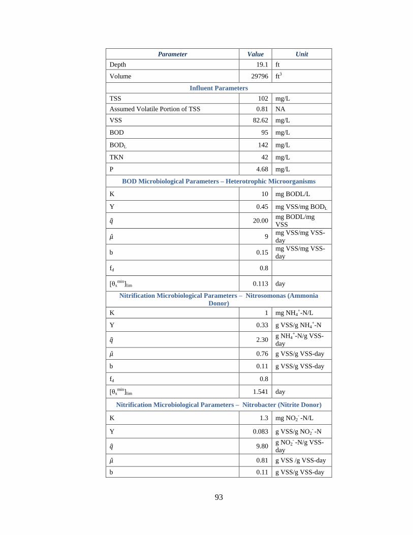
93
Parameter Value Unit
Depth 19.1 ft
Volume 29796 ft3
Influent Parameters
TSS 102 mg/L
Assumed Volatile Portion of TSS 0.81 NA
VSS 82.62 mg/L
BOD 95 mg/L
BODL 142 mg/L
TKN 42 mg/L
P 4.68 mg/L
BOD Microbiological Parameters – Heterotrophic Microorganisms
K 10 mg BODL/L
Y 0.45 mg VSS/mg BODL
20.00 mg BODL/mg
VSS
9 mg VSS/mg VSS-
day
b 0.15 mg VSS/mg VSS-
day
fd 0.8
[θxmin]lim 0.113 day
Nitrification Microbiological Parameters – Nitrosomonas (Ammonia
Donor)
K 1 mg NH4+-N/L
Y 0.33 g VSS/g NH4+-N
2.30 g NH4
+-N/g VSS-
day
0.76 g VSS/g VSS-day
b 0.11 g VSS/g VSS-day
fd 0.8
[θxmin]lim 1.541 day
Nitrification Microbiological Parameters – Nitrobacter (Nitrite Donor)
K 1.3 mg NO2- -N/L
Y 0.083 g VSS/g NO2- -N
9.80 g NO2
- -N/g VSS-
day
0.81 g VSS /g VSS-day
b 0.11 g VSS/g VSS-day
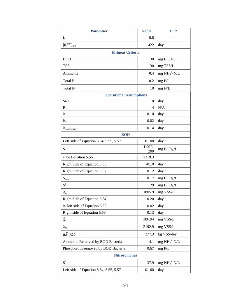
94
Parameter Value Unit
fd 0.8
[θxmin]lim 1.422 day
Effluent Criteria
BOD 30 mg BOD/L
TSS 30 mg TSS/L
Ammonia 0.4 mg NH4+-N/L
Total P 0.2 mg P/L
Total N 10 mg N/L
Operational Assumptions
SRT 10 day
R1 4 N/A
θ 0.10 day
θr 0.02 day
θtotalsystem 0.14 day
BOD
Left side of Equation 5.54, 5.55, 5.57 0.100 day-1
S 1.00E-
200 mg BODL/L
e for Equation 5.55 2319.3
Right Side of Equation 5.55 -0.10 day-1
Right Side of Equation 5.57 0.12 day-1
Smin 0.17 mg BODL/L
Si 29 mg BODL/L
1805.9 mg VSS/L
Right Side of Equation 5.54 0.20 day-1
θr left side of Equation 5.53 0.02 day
Right side of Equation 5.53 0.13 day
386.94 mg VSS/L
2192.9 mg VSS/L
277.3 kg VSS/day
Ammonia Removed by BOD Bacteria 4.1 mg NH4+-N/L
Phosphorous removed by BOD Bacteria 0.67 mg P/L
Nitrosomonas
S0 37.9 mg NH4+-N/L
Left side of Equation 5.54, 5.55, 5.57 0.100 day-1
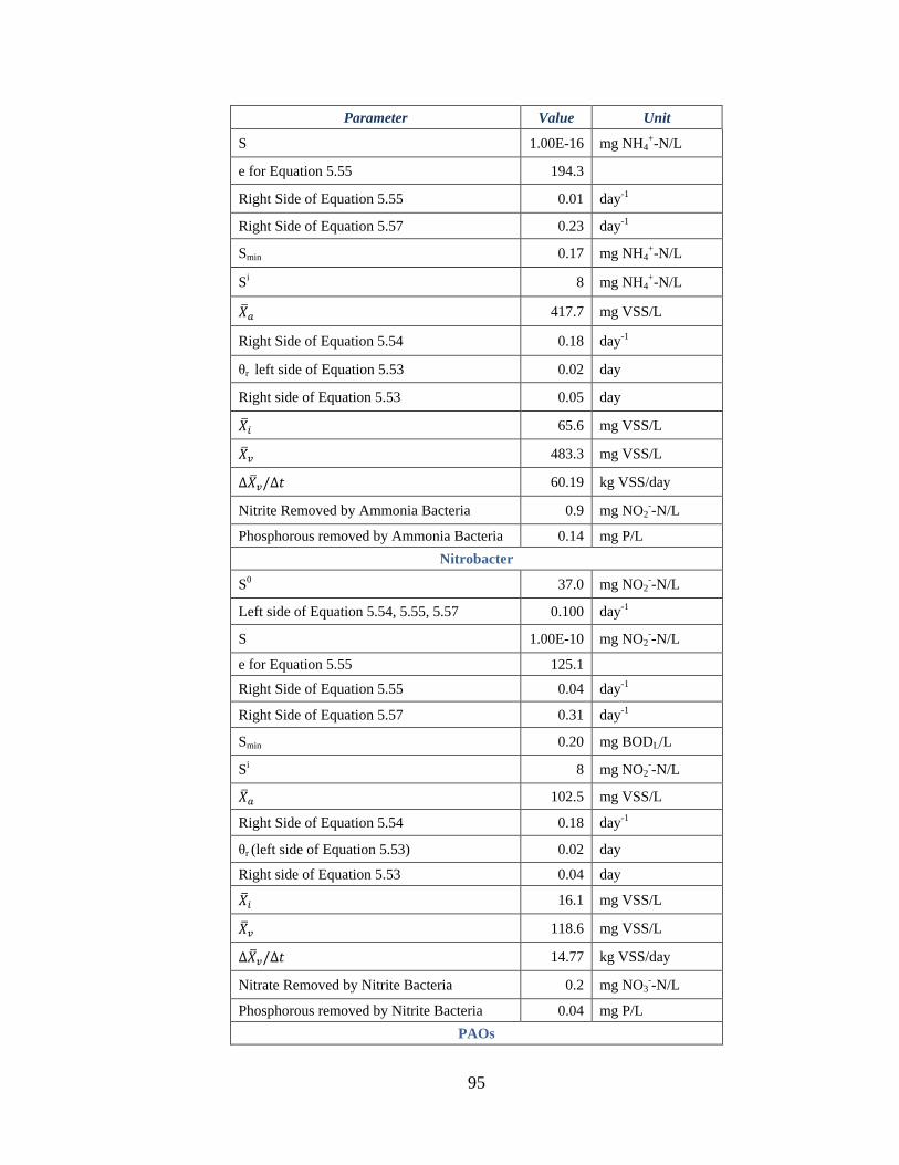
95
Parameter Value Unit
S 1.00E-16 mg NH4+-N/L
e for Equation 5.55 194.3
Right Side of Equation 5.55 0.01 day-1
Right Side of Equation 5.57 0.23 day-1
Smin 0.17 mg NH4+-N/L
Si 8 mg NH4+-N/L
417.7 mg VSS/L
Right Side of Equation 5.54 0.18 day-1
θr left side of Equation 5.53 0.02 day
Right side of Equation 5.53 0.05 day
65.6 mg VSS/L
483.3 mg VSS/L
60.19 kg VSS/day
Nitrite Removed by Ammonia Bacteria 0.9 mg NO2--N/L
Phosphorous removed by Ammonia Bacteria 0.14 mg P/L
Nitrobacter
S0 37.0 mg NO2--N/L
Left side of Equation 5.54, 5.55, 5.57 0.100 day-1
S 1.00E-10 mg NO2--N/L
e for Equation 5.55 125.1
Right Side of Equation 5.55 0.04 day-1
Right Side of Equation 5.57 0.31 day-1
Smin 0.20 mg BODL/L
Si 8 mg NO2--N/L
102.5 mg VSS/L
Right Side of Equation 5.54 0.18 day-1
θr (left side of Equation 5.53) 0.02 day
Right side of Equation 5.53 0.04 day
16.1 mg VSS/L
118.6 mg VSS/L
14.77 kg VSS/day
Nitrate Removed by Nitrite Bacteria 0.2 mg NO3--N/L
Phosphorous removed by Nitrite Bacteria 0.04 mg P/L
PAOs

96
Parameter Value Unit
– aerobic zone due to recycle 649 mg VSS/L
– aerobic zone due to recycle 51.9 mg VSS/L
700.9 mg VSS/L
82.8 kg VSS/day
Phosphorous removed by PAO Bacteria 2.98 mg P/L
Nitrate Removed by PAO Bacteria 1.2 mg NO3--N/L
Effluent
Phosphorous Effluent Estimated (Rittmann, et
al., 2001) 0.74 mg P/L
Total Influent COD 250.00 mg COD/L
fus 0.05 mg/mg COD
fup 0.13 mg/mg COD
fcv 1.48 mg COD/mg VSS
bhT 0.24 g VSS/g VSS-day
SRT 10.00 days
Yh 0.45 mg VSS/mg COD
γ -0.21 mg P/mg VSS
Pf 2.70
Sbsa 43.00 mg/L
fxa 0.15
fp 0.015 mg P/mg VSS
f 0.2 mg/mg VSS
Part 1 of Equation 15.15 (WEF, 2010a) -2.2E-02
Part 2 of Equation 15.15 1.3E-03
Phosphorous Removal Estimated by Equation
15.15 -5.10 mg P/L
Effluent P by Equation 15.15 0 mg P/L
P Removal by Figure 15.45 (WEF, 2010a) 0.017 mg P/mg COD
P Removal by Figure 15.45 4.250 mg P/L
Effluent P by Figure 15.45 0 mg P/L
Reactive Nitrate In Influent for P Reactor 1.208 mg/L
rbCOD/nitrate ratio 6.6 g rbCOD/g Nitrate
rbCOD (VFA) 43 mg/L
rbCOD Equivalent 7.98 mg/L
rbCOD available for P Removal 35.03 mg/L
rbCOD/P Ratio 10 g rbCOD/g P
Biological P Removal 3.50 mg/L
P Removal by other Bacteria 0.96 mg/L
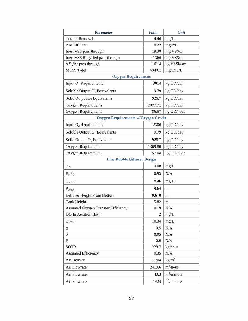
97
Parameter Value Unit
Total P Removal 4.46 mg/L
P in Effluent 0.22 mg P/L
Inert VSS pass through 19.38 mg VSS/L
Inert VSS Recycled pass through 1366 mg VSS/L
pass through 161.4 kg VSSi/day
MLSS Total 6340.1 mg TSS/L
Oxygen Requirements
Input O2 Requirements 3014 kg OD/day
Soluble Output O2 Equivalents 9.79 kg OD/day
Solid Output O2 Equivalents 926.7 kg OD/day
Oxygen Requirements 2077.71 kg OD/day
Oxygen Requirements 86.57 kg OD/hour
Oxygen Requirements w/Oxygen Credit
Input O2 Requirements 2306 kg OD/day
Soluble Output O2 Equivalents 9.79 kg OD/day
Solid Output O2 Equivalents 926.7 kg OD/day
Oxygen Requirements 1369.80 kg OD/day
Oxygen Requirements 57.08 kg OD/hour
Fine Bubble Diffuser Design
C20 9.08 mg/L
Pb/Pa 0.93 N/A
Cs,T,H 8.46 mg/L
Patm,H 9.64 m
Diffuser Height From Bottom 0.610 m
Tank Height 5.82 m
Assumed Oxygen Transfer Efficiency 0.19 N/A
DO In Aeration Basin 2 mg/L
Cs,T,H 10.34 mg/L
α 0.5 N/A
β 0.95 N/A
F 0.9 N/A
SOTR 228.7 kg/hour
Assumed Efficiency 0.35 N/A
Air Density 1.204 kg/m3
Air Flowrate 2419.6 m3/hour
Air Flowrate 40.3 m3/minute
Air Flowrate 1424 ft3/minute
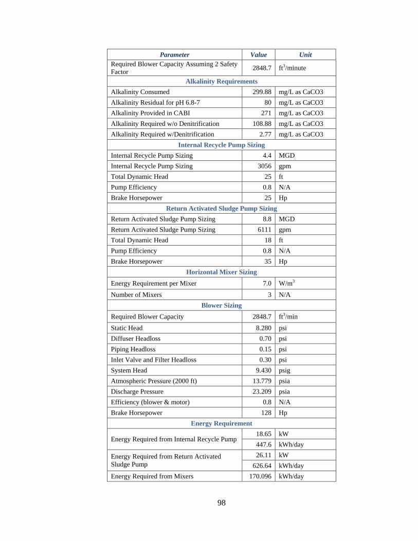
98
Parameter Value Unit
Required Blower Capacity Assuming 2 Safety
Factor 2848.7 ft3/minute
Alkalinity Requirements
Alkalinity Consumed 299.88 mg/L as CaCO3
Alkalinity Residual for pH 6.8-7 80 mg/L as CaCO3
Alkalinity Provided in CABI 271 mg/L as CaCO3
Alkalinity Required w/o Denitrification 108.88 mg/L as CaCO3
Alkalinity Required w/Denitrification 2.77 mg/L as CaCO3
Internal Recycle Pump Sizing
Internal Recycle Pump Sizing 4.4 MGD
Internal Recycle Pump Sizing 3056 gpm
Total Dynamic Head 25 ft
Pump Efficiency 0.8 N/A
Brake Horsepower 25 Hp
Return Activated Sludge Pump Sizing
Return Activated Sludge Pump Sizing 8.8 MGD
Return Activated Sludge Pump Sizing 6111 gpm
Total Dynamic Head 18 ft
Pump Efficiency 0.8 N/A
Brake Horsepower 35 Hp
Horizontal Mixer Sizing
Energy Requirement per Mixer 7.0 W/m3
Number of Mixers 3 N/A
Blower Sizing
Required Blower Capacity 2848.7 ft3/min
Static Head 8.280 psi
Diffuser Headloss 0.70 psi
Piping Headloss 0.15 psi
Inlet Valve and Filter Headloss 0.30 psi
System Head 9.430 psig
Atmospheric Pressure (2000 ft) 13.779 psia
Discharge Pressure 23.209 psia
Efficiency (blower & motor) 0.8 N/A
Brake Horsepower 128 Hp
Energy Requirement
Energy Required from Internal Recycle Pump 18.65 kW
447.6 kWh/day
Energy Required from Return Activated
Sludge Pump
26.11 kW
626.64 kWh/day
Energy Required from Mixers 170.096 kWh/day
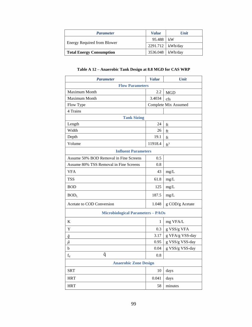
99
Parameter Value Unit
Energy Required from Blower 95.488 kW
2291.712 kWh/day
Total Energy Consumption 3536.048 kWh/day
Table A 12 – Anaerobic Tank Design at 8.8 MGD for CAS WRP
Parameter Value Unit
Flow Parameters
Maximum Month 2.2 MGD
Maximum Month 3.4034 cfs
Flow Type Complete Mix Assumed
4 Trains
Tank Sizing
Length 24 ft
Width 26 ft
Depth 19.1 ft
Volume 11918.4 ft3
Influent Parameters
Assume 50% BOD Removal in Fine Screens 0.5
Assume 80% TSS Removal in Fine Screens 0.8
VFA 43 mg/L
TSS 61.8 mg/L
BOD 125 mg/L
BODL 187.5 mg/L
Acetate to COD Conversion 1.048 g COD/g Acetate
Microbiological Parameters – PAOs
K 1 mg VFA/L
Y 0.3 g VSS/g VFA
3.17 g VFA/g VSS-day
0.95 g VSS/g VSS-day
b 0.04 g VSS/g VSS-day
fd 0.8
Anaerobic Zone Design
SRT 10 days
HRT 0.041 days
HRT 58 minutes
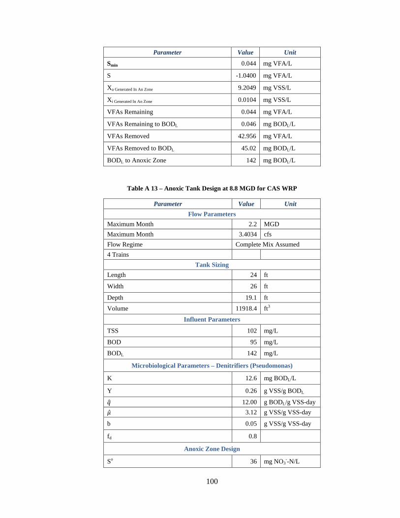
100
Parameter Value Unit
Smin 0.044 mg VFA/L
S -1.0400 mg VFA/L
Xa Generated In An Zone 9.2049 mg VSS/L
Xi Generated In An Zone 0.0104 mg VSS/L
VFAs Remaining 0.044 mg VFA/L
VFAs Remaining to BODL 0.046 mg BODL/L
VFAs Removed 42.956 mg VFA/L
VFAs Removed to BODL 45.02 mg BODL/L
BODL to Anoxic Zone 142 mg BODL/L
Table A 13 – Anoxic Tank Design at 8.8 MGD for CAS WRP
Parameter Value Unit
Flow Parameters
Maximum Month 2.2 MGD
Maximum Month 3.4034 cfs
Flow Regime Complete Mix Assumed
4 Trains
Tank Sizing
Length 24 ft
Width 26 ft
Depth 19.1 ft
Volume 11918.4 ft3
Influent Parameters
TSS 102 mg/L
BOD 95 mg/L
BODL 142 mg/L
Microbiological Parameters – Denitrifiers (Pseudomonas)
K 12.6 mg BODL/L
Y 0.26 g VSS/g BODL
12.00 g BODL/g VSS-day
3.12 g VSS/g VSS-day
b 0.05 g VSS/g VSS-day
fd 0.8
Anoxic Zone Design
So 36 mg NO3--N/L
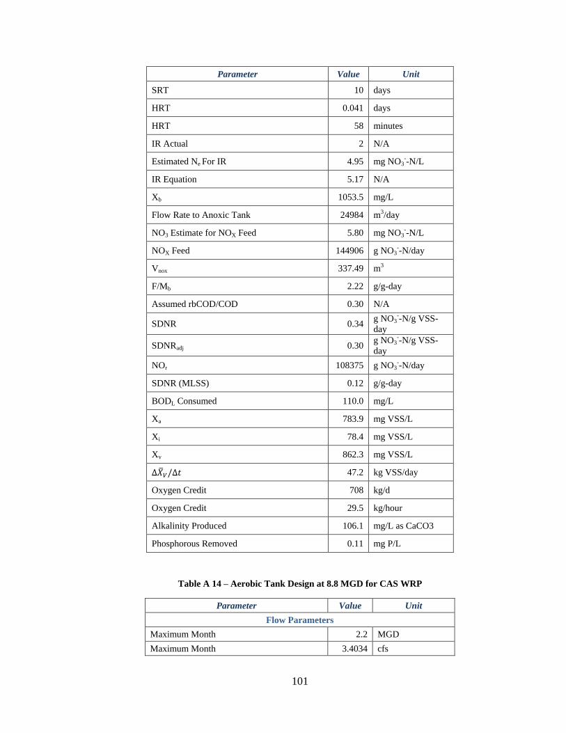
101
Parameter Value Unit
SRT 10 days
HRT 0.041 days
HRT 58 minutes
IR Actual 2 N/A
Estimated Ne For IR 4.95 mg NO3--N/L
IR Equation 5.17 N/A
Xb 1053.5 mg/L
Flow Rate to Anoxic Tank 24984 m3/day
NO3 Estimate for NOX Feed 5.80 mg NO3--N/L
NOX Feed 144906 g NO3--N/day
Vnox 337.49 m3
F/Mb 2.22 g/g-day
Assumed rbCOD/COD 0.30 N/A
SDNR 0.34 g NO3
--N/g VSS-
day
SDNRadj 0.30 g NO3
--N/g VSS-
day
NOr 108375 g NO3--N/day
SDNR (MLSS) 0.12 g/g-day
BODL Consumed 110.0 mg/L
Xa 783.9 mg VSS/L
Xi 78.4 mg VSS/L
Xv 862.3 mg VSS/L
47.2 kg VSS/day
Oxygen Credit 708 kg/d
Oxygen Credit 29.5 kg/hour
Alkalinity Produced 106.1 mg/L as CaCO3
Phosphorous Removed 0.11 mg P/L
Table A 14 – Aerobic Tank Design at 8.8 MGD for CAS WRP
Parameter Value Unit
Flow Parameters
Maximum Month 2.2 MGD
Maximum Month 3.4034 cfs
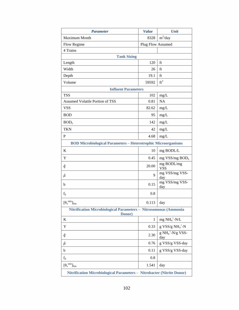
102
Parameter Value Unit
Maximum Month 8328 m3/day
Flow Regime Plug Flow Assumed
4 Trains
Tank Sizing
Length 120 ft
Width 26 ft
Depth 19.1 ft
Volume 59592 ft3
Influent Parameters
TSS 102 mg/L
Assumed Volatile Portion of TSS 0.81 NA
VSS 82.62 mg/L
BOD 95 mg/L
BODL 142 mg/L
TKN 42 mg/L
P 4.68 mg/L
BOD Microbiological Parameters – Heterotrophic Microorganisms
K 10 mg BODL/L
Y 0.45 mg VSS/mg BODL
20.00 mg BODL/mg
VSS
9 mg VSS/mg VSS-
day
b 0.15 mg VSS/mg VSS-
day
fd 0.8
[θxmin]lim 0.113 day
Nitrification Microbiological Parameters – Nitrosomonas (Ammonia
Donor)
K 1 mg NH4+-N/L
Y 0.33 g VSS/g NH4+-N
2.30 g NH4
+-N/g VSS-
day
0.76 g VSS/g VSS-day
b 0.11 g VSS/g VSS-day
fd 0.8
[θxmin]lim 1.541 day
Nitrification Microbiological Parameters – Nitrobacter (Nitrite Donor)
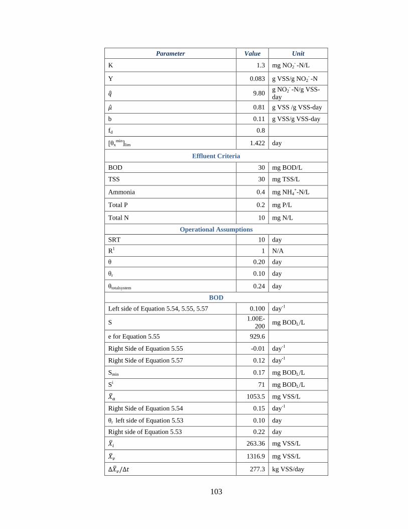
103
Parameter Value Unit
K 1.3 mg NO2- -N/L
Y 0.083 g VSS/g NO2- -N
9.80 g NO2
- -N/g VSS-
day
0.81 g VSS /g VSS-day
b 0.11 g VSS/g VSS-day
fd 0.8
[θxmin]lim 1.422 day
Effluent Criteria
BOD 30 mg BOD/L
TSS 30 mg TSS/L
Ammonia 0.4 mg NH4+-N/L
Total P 0.2 mg P/L
Total N 10 mg N/L
Operational Assumptions
SRT 10 day
R1 1 N/A
θ 0.20 day
θr 0.10 day
θtotalsystem 0.24 day
BOD
Left side of Equation 5.54, 5.55, 5.57 0.100 day-1
S 1.00E-
200 mg BODL/L
e for Equation 5.55 929.6
Right Side of Equation 5.55 -0.01 day-1
Right Side of Equation 5.57 0.12 day-1
Smin 0.17 mg BODL/L
Si 71 mg BODL/L
1053.5 mg VSS/L
Right Side of Equation 5.54 0.15 day-1
θr left side of Equation 5.53 0.10 day
Right side of Equation 5.53 0.22 day
263.36 mg VSS/L
1316.9 mg VSS/L
277.3 kg VSS/day

104
Parameter Value Unit
Ammonia Removed by BOD Bacteria 4.1 mg NH4+-N/L
Phosphorous removed by BOD Bacteria 0.67 mg P/L
Nitrosomonas
S0 37.9 mg NH4+-N/L
Left side of Equation 5.54, 5.55, 5.57 0.100 day-1
S 1.00E-16 mg NH4+-N/L
e for Equation 5.55 79.6
Right Side of Equation 5.55 0.13 day-1
Right Side of Equation 5.57 0.23 day-1
Smin 0.17 mg NH4+-N/L
Si 19 mg NH4+-N/L
243.7 mg VSS/L
Right Side of Equation 5.54 0.14 day-1
θr left side of Equation 5.53 0.10 day
Right side of Equation 5.53 0.10 day
44.7 mg VSS/L
288.3 mg VSS/L
60.19 kg VSS/day
Nitrite Removed by Ammonia Bacteria 0.9 mg NO2--N/L
Phosphorous removed by Ammonia Bacteria 0.14 mg P/L
Nitrobacter
S0 37.0 mg NO2--N/L
Left side of Equation 5.54, 5.55, 5.57 0.100 day-1
S 1.00E-10 mg NO2--N/L
e for Equation 5.55 51.9
Right Side of Equation 5.55 0.18 day-1
Right Side of Equation 5.57 0.31 day-1
Smin 0.20 mg BODL/L
Si 19 mg NO2--N/L
59.8 mg VSS/L
Right Side of Equation 5.54 0.14 day-1
θr (left side of Equation 5.53) 0.10 day
Right side of Equation 5.53 0.09 day
11.0 mg VSS/L
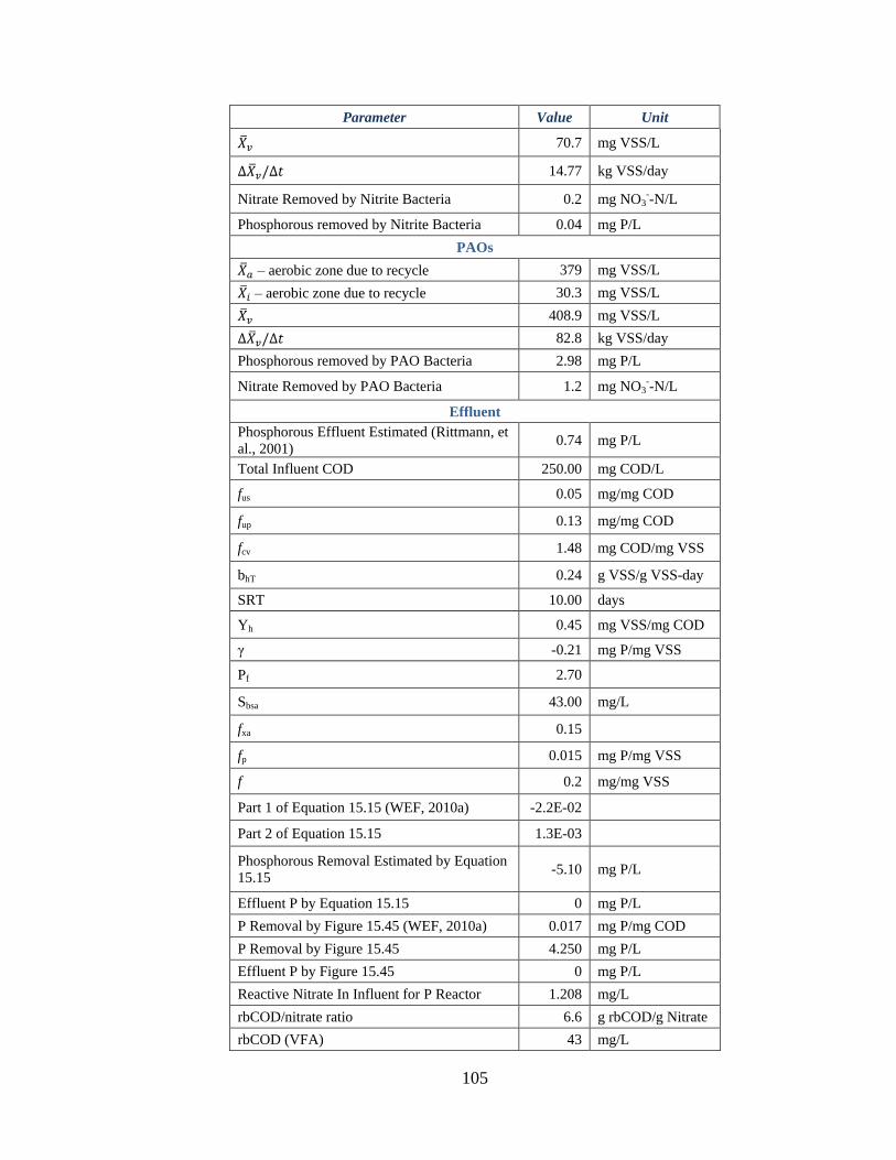
105
Parameter Value Unit
70.7 mg VSS/L
14.77 kg VSS/day
Nitrate Removed by Nitrite Bacteria 0.2 mg NO3--N/L
Phosphorous removed by Nitrite Bacteria 0.04 mg P/L
PAOs
– aerobic zone due to recycle 379 mg VSS/L
– aerobic zone due to recycle 30.3 mg VSS/L
408.9 mg VSS/L
82.8 kg VSS/day
Phosphorous removed by PAO Bacteria 2.98 mg P/L
Nitrate Removed by PAO Bacteria 1.2 mg NO3--N/L
Effluent
Phosphorous Effluent Estimated (Rittmann, et
al., 2001) 0.74 mg P/L
Total Influent COD 250.00 mg COD/L
fus 0.05 mg/mg COD
fup 0.13 mg/mg COD
fcv 1.48 mg COD/mg VSS
bhT 0.24 g VSS/g VSS-day
SRT 10.00 days
Yh 0.45 mg VSS/mg COD
γ -0.21 mg P/mg VSS
Pf 2.70
Sbsa 43.00 mg/L
fxa 0.15
fp 0.015 mg P/mg VSS
f 0.2 mg/mg VSS
Part 1 of Equation 15.15 (WEF, 2010a) -2.2E-02
Part 2 of Equation 15.15 1.3E-03
Phosphorous Removal Estimated by Equation
15.15 -5.10 mg P/L
Effluent P by Equation 15.15 0 mg P/L
P Removal by Figure 15.45 (WEF, 2010a) 0.017 mg P/mg COD
P Removal by Figure 15.45 4.250 mg P/L
Effluent P by Figure 15.45 0 mg P/L
Reactive Nitrate In Influent for P Reactor 1.208 mg/L
rbCOD/nitrate ratio 6.6 g rbCOD/g Nitrate
rbCOD (VFA) 43 mg/L
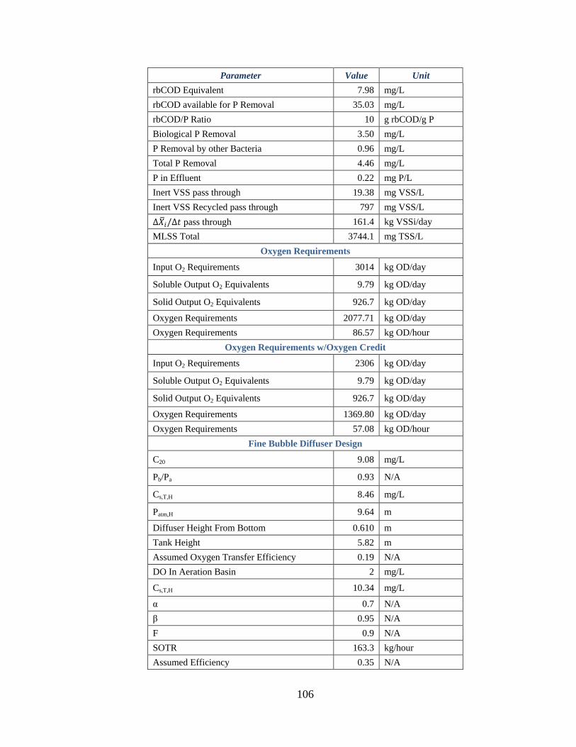
106
Parameter Value Unit
rbCOD Equivalent 7.98 mg/L
rbCOD available for P Removal 35.03 mg/L
rbCOD/P Ratio 10 g rbCOD/g P
Biological P Removal 3.50 mg/L
P Removal by other Bacteria 0.96 mg/L
Total P Removal 4.46 mg/L
P in Effluent 0.22 mg P/L
Inert VSS pass through 19.38 mg VSS/L
Inert VSS Recycled pass through 797 mg VSS/L
pass through 161.4 kg VSSi/day
MLSS Total 3744.1 mg TSS/L
Oxygen Requirements
Input O2 Requirements 3014 kg OD/day
Soluble Output O2 Equivalents 9.79 kg OD/day
Solid Output O2 Equivalents 926.7 kg OD/day
Oxygen Requirements 2077.71 kg OD/day
Oxygen Requirements 86.57 kg OD/hour
Oxygen Requirements w/Oxygen Credit
Input O2 Requirements 2306 kg OD/day
Soluble Output O2 Equivalents 9.79 kg OD/day
Solid Output O2 Equivalents 926.7 kg OD/day
Oxygen Requirements 1369.80 kg OD/day
Oxygen Requirements 57.08 kg OD/hour
Fine Bubble Diffuser Design
C20 9.08 mg/L
Pb/Pa 0.93 N/A
Cs,T,H 8.46 mg/L
Patm,H 9.64 m
Diffuser Height From Bottom 0.610 m
Tank Height 5.82 m
Assumed Oxygen Transfer Efficiency 0.19 N/A
DO In Aeration Basin 2 mg/L
Cs,T,H 10.34 mg/L
α 0.7 N/A
β 0.95 N/A
F 0.9 N/A
SOTR 163.3 kg/hour
Assumed Efficiency 0.35 N/A
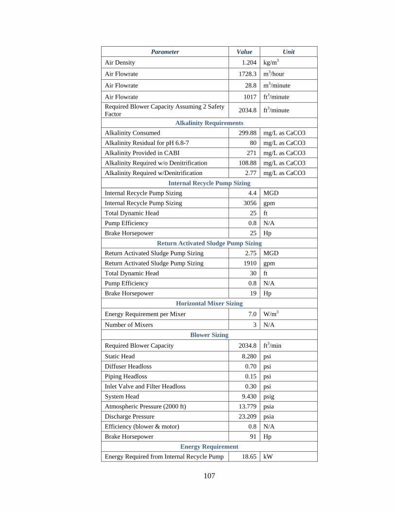
107
Parameter Value Unit
Air Density 1.204 kg/m3
Air Flowrate 1728.3 m3/hour
Air Flowrate 28.8 m3/minute
Air Flowrate 1017 ft3/minute
Required Blower Capacity Assuming 2 Safety
Factor 2034.8 ft3/minute
Alkalinity Requirements
Alkalinity Consumed 299.88 mg/L as CaCO3
Alkalinity Residual for pH 6.8-7 80 mg/L as CaCO3
Alkalinity Provided in CABI 271 mg/L as CaCO3
Alkalinity Required w/o Denitrification 108.88 mg/L as CaCO3
Alkalinity Required w/Denitrification 2.77 mg/L as CaCO3
Internal Recycle Pump Sizing
Internal Recycle Pump Sizing 4.4 MGD
Internal Recycle Pump Sizing 3056 gpm
Total Dynamic Head 25 ft
Pump Efficiency 0.8 N/A
Brake Horsepower 25 Hp
Return Activated Sludge Pump Sizing
Return Activated Sludge Pump Sizing 2.75 MGD
Return Activated Sludge Pump Sizing 1910 gpm
Total Dynamic Head 30 ft
Pump Efficiency 0.8 N/A
Brake Horsepower 19 Hp
Horizontal Mixer Sizing
Energy Requirement per Mixer 7.0 W/m3
Number of Mixers 3 N/A
Blower Sizing
Required Blower Capacity 2034.8 ft3/min
Static Head 8.280 psi
Diffuser Headloss 0.70 psi
Piping Headloss 0.15 psi
Inlet Valve and Filter Headloss 0.30 psi
System Head 9.430 psig
Atmospheric Pressure (2000 ft) 13.779 psia
Discharge Pressure 23.209 psia
Efficiency (blower & motor) 0.8 N/A
Brake Horsepower 91 Hp
Energy Requirement
Energy Required from Internal Recycle Pump 18.65 kW

108
Parameter Value Unit
447.6 kWh/day
Energy Required from Return Activated
Sludge Pump
14.17 kW
340.18 kWh/day
Energy Required from Mixers 170.096 kWh/day
Energy Required from Blower 67.886 kW
1629.264 kWh/day
Total Energy Consumption 2587.136 kWh/day
A-5 Membranes
Parameters used in the design of the membrane portion of the MBR system can be found
in Table A 15.
Table A 15 – Membrane Filtration Design Parameters
Parameter Value Unit Reference
RAS recycle ratio 400-500 % (WEF, 2012)
MLSSmembrane tank 8,000-12,000 mg/L (WEF, 2012)
Design peak-day flux 13.5 gal/ft2/day (Menniti, et al.,
2011)
Design average-day flux 12.9 gal/ft2/day (Menniti, et al.,
2011)
Spare membrane area ratio 10 % (WEF, 2012)
Membrane area per small subunit 32 m2 (WEF, 2012)
Number of small subunits per large
membrane subunit 48 – (WEF, 2012)
Volume required for each large subunit 20 m3 (WEF, 2012)
Air scour rate at average-day flowrate 10/30 seconds on/
seconds off (WEF, 2012)
Air scour rate at peak-day flowrate 10/10 seconds on/
seconds off (WEF, 2012)
Online factor including relaxation
interval and maintenance cleaning 95 % (WEF, 2012)
Air scour flowrate at average-day per
small subunit 10 Nm3/hr (WEF, 2012)
Air scour flowrate at peak-day per
small subunit 20 Nm3/hr (WEF, 2012)
To determine the MLSS concentration inside the membrane tank the following equation
was used
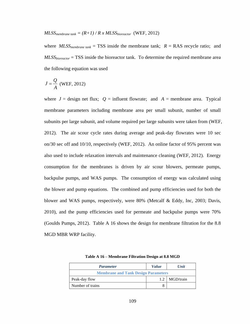
109
MLSSmembrane tank = (R+1) / R x MLSSbioreactor (WEF, 2012)
where MLSSmembrane tank = TSS inside the membrane tank; R = RAS recycle ratio; and
MLSSbioreactor = TSS inside the bioreactor tank. To determine the required membrane area
the following equation was used
A
QJ (WEF, 2012)
where J = design net flux; Q = influent flowrate; and A = membrane area. Typical
membrane parameters including membrane area per small subunit, number of small
subunits per large subunit, and volume required per large subunits were taken from (WEF,
2012). The air scour cycle rates during average and peak-day flowrates were 10 sec
on/30 sec off and 10/10, respectively (WEF, 2012). An online factor of 95% percent was
also used to include relaxation intervals and maintenance cleaning (WEF, 2012). Energy
consumption for the membranes is driven by air scour blowers, permeate pumps,
backpulse pumps, and WAS pumps. The consumption of energy was calculated using
the blower and pump equations. The combined and pump efficiencies used for both the
blower and WAS pumps, respectively, were 80% (Metcalf & Eddy, Inc, 2003; Davis,
2010), and the pump efficiencies used for permeate and backpulse pumps were 70%
(Goulds Pumps, 2012). Table A 16 shows the design for membrane filtration for the 8.8
MGD MBR WRP facility.
Table A 16 – Membrane Filtration Design at 8.8 MGD
Parameter Value Unit
Membrane and Tank Design Parameters
Peak-day flow 1.2 MGD/train
Number of trains 8
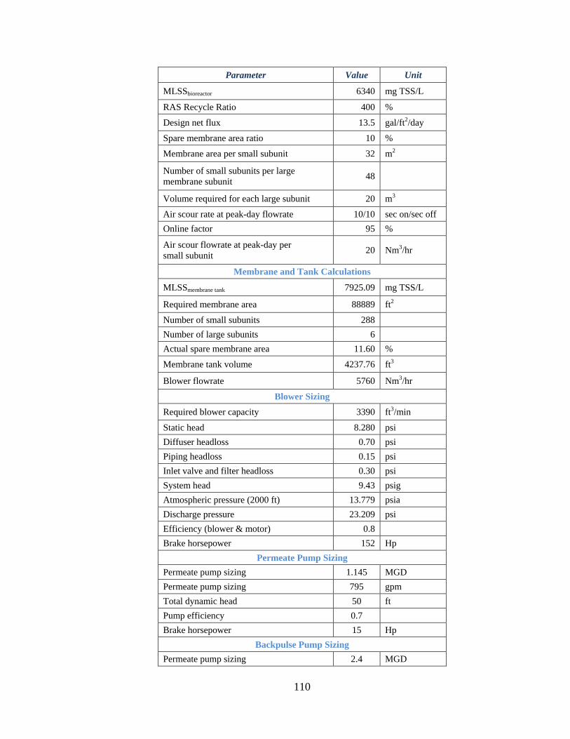
110
Parameter Value Unit
MLSSbioreactor 6340 mg TSS/L
RAS Recycle Ratio 400 %
Design net flux 13.5 gal/ft2/day
Spare membrane area ratio 10 %
Membrane area per small subunit 32 m2
Number of small subunits per large
membrane subunit 48
Volume required for each large subunit 20 m3
Air scour rate at peak-day flowrate 10/10 sec on/sec off
Online factor 95 %
Air scour flowrate at peak-day per
small subunit 20 Nm3/hr
Membrane and Tank Calculations
MLSSmembrane tank 7925.09 mg TSS/L
Required membrane area 88889 ft2
Number of small subunits 288
Number of large subunits 6
Actual spare membrane area 11.60 %
Membrane tank volume 4237.76 ft3
Blower flowrate 5760 Nm3/hr
Blower Sizing
Required blower capacity 3390 ft3/min
Static head 8.280 psi
Diffuser headloss 0.70 psi
Piping headloss 0.15 psi
Inlet valve and filter headloss 0.30 psi
System head 9.43 psig
Atmospheric pressure (2000 ft) 13.779 psia
Discharge pressure 23.209 psi
Efficiency (blower & motor) 0.8
Brake horsepower 152 Hp
Permeate Pump Sizing
Permeate pump sizing 1.145 MGD
Permeate pump sizing 795 gpm
Total dynamic head 50 ft
Pump efficiency 0.7
Brake horsepower 15 Hp
Backpulse Pump Sizing
Permeate pump sizing 2.4 MGD
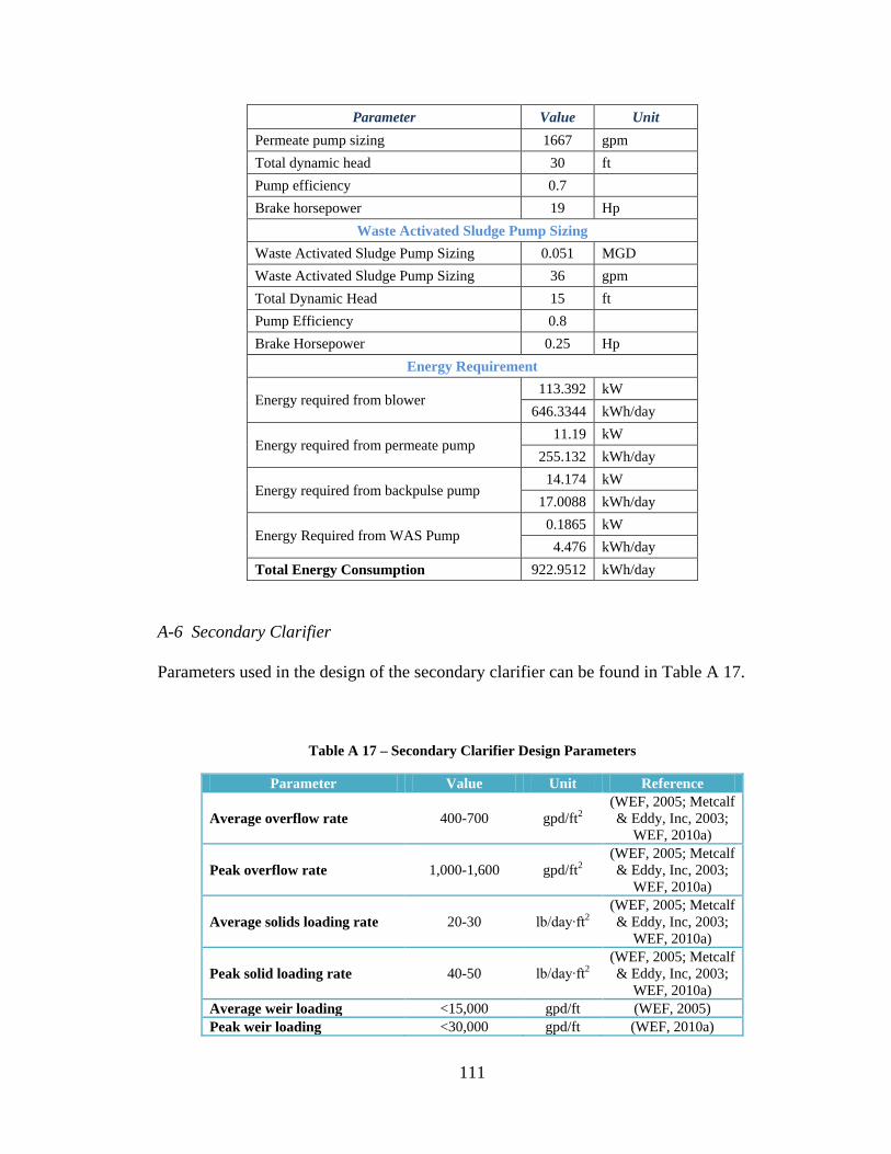
111
Parameter Value Unit
Permeate pump sizing 1667 gpm
Total dynamic head 30 ft
Pump efficiency 0.7
Brake horsepower 19 Hp
Waste Activated Sludge Pump Sizing
Waste Activated Sludge Pump Sizing 0.051 MGD
Waste Activated Sludge Pump Sizing 36 gpm
Total Dynamic Head 15 ft
Pump Efficiency 0.8
Brake Horsepower 0.25 Hp
Energy Requirement
Energy required from blower 113.392 kW
646.3344 kWh/day
Energy required from permeate pump 11.19 kW
255.132 kWh/day
Energy required from backpulse pump 14.174 kW
17.0088 kWh/day
Energy Required from WAS Pump 0.1865 kW
4.476 kWh/day
Total Energy Consumption 922.9512 kWh/day
A-6 Secondary Clarifier
Parameters used in the design of the secondary clarifier can be found in Table A 17.
Table A 17 – Secondary Clarifier Design Parameters
Parameter Value Unit Reference
Average overflow rate 400-700 gpd/ft2
(WEF, 2005; Metcalf
& Eddy, Inc, 2003;
WEF, 2010a)
Peak overflow rate 1,000-1,600 gpd/ft2
(WEF, 2005; Metcalf
& Eddy, Inc, 2003;
WEF, 2010a)
Average solids loading rate 20-30 lb/day∙ft2
(WEF, 2005; Metcalf
& Eddy, Inc, 2003;
WEF, 2010a)
Peak solid loading rate 40-50 lb/day∙ft2
(WEF, 2005; Metcalf
& Eddy, Inc, 2003;
WEF, 2010a)
Average weir loading <15,000 gpd/ft (WEF, 2005)
Peak weir loading <30,000 gpd/ft (WEF, 2010a)
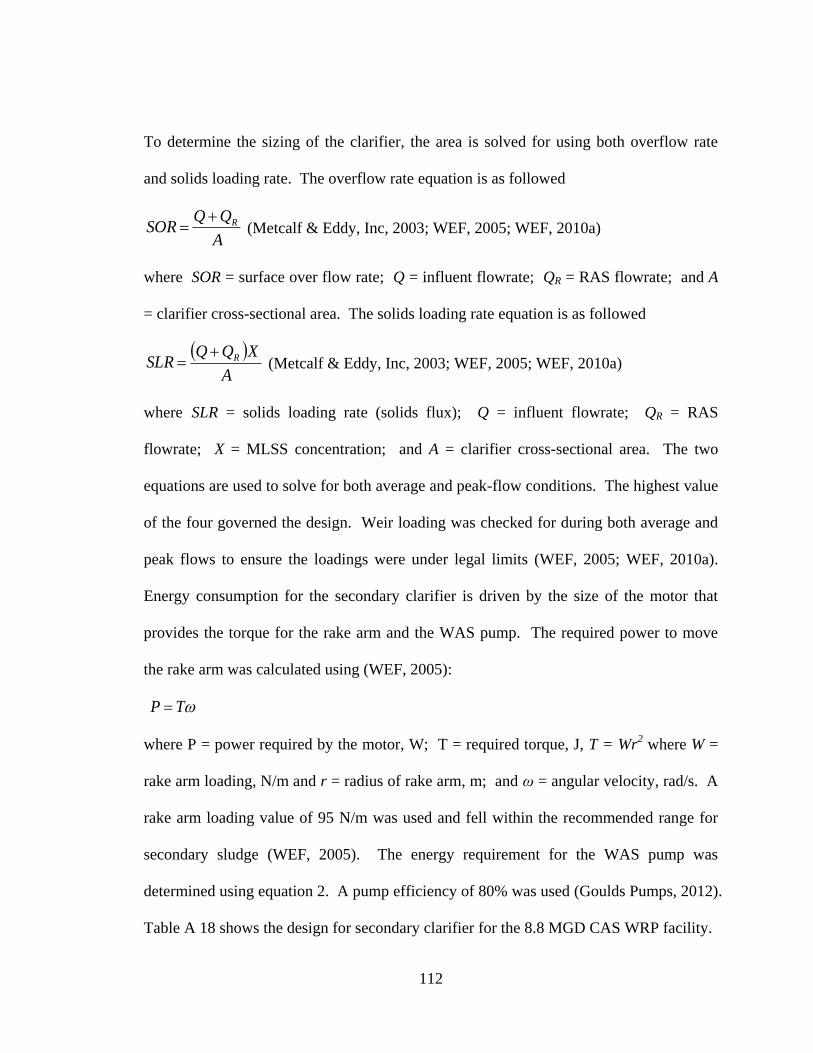
112
To determine the sizing of the clarifier, the area is solved for using both overflow rate
and solids loading rate. The overflow rate equation is as followed
A
QQSOR R
(Metcalf & Eddy, Inc, 2003; WEF, 2005; WEF, 2010a)
where SOR = surface over flow rate; Q = influent flowrate; QR = RAS flowrate; and A
= clarifier cross-sectional area. The solids loading rate equation is as followed
A
XQQSLR R
(Metcalf & Eddy, Inc, 2003; WEF, 2005; WEF, 2010a)
where SLR = solids loading rate (solids flux); Q = influent flowrate; QR = RAS
flowrate; X = MLSS concentration; and A = clarifier cross-sectional area. The two
equations are used to solve for both average and peak-flow conditions. The highest value
of the four governed the design. Weir loading was checked for during both average and
peak flows to ensure the loadings were under legal limits (WEF, 2005; WEF, 2010a).
Energy consumption for the secondary clarifier is driven by the size of the motor that
provides the torque for the rake arm and the WAS pump. The required power to move
the rake arm was calculated using (WEF, 2005):
TP
where P = power required by the motor, W; T = required torque, J, T = Wr2 where W =
rake arm loading, N/m and r = radius of rake arm, m; and ω = angular velocity, rad/s. A
rake arm loading value of 95 N/m was used and fell within the recommended range for
secondary sludge (WEF, 2005). The energy requirement for the WAS pump was
determined using equation 2. A pump efficiency of 80% was used (Goulds Pumps, 2012).
Table A 18 shows the design for secondary clarifier for the 8.8 MGD CAS WRP facility.
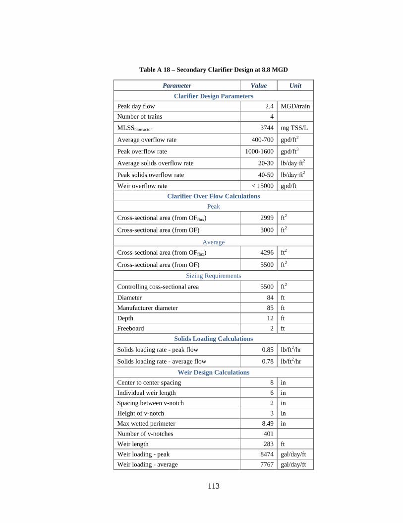
113
Table A 18 – Secondary Clarifier Design at 8.8 MGD
Parameter Value Unit
Clarifier Design Parameters
Peak day flow 2.4 MGD/train
Number of trains 4
MLSSbioreactor 3744 mg TSS/L
Average overflow rate 400-700 gpd/ft2
Peak overflow rate 1000-1600 gpd/ft3
Average solids overflow rate 20-30 lb/day∙ft2
Peak solids overflow rate 40-50 lb/day∙ft2
Weir overflow rate < 15000 gpd/ft
Clarifier Over Flow Calculations
Peak
Cross-sectional area (from OFflux) 2999 ft2
Cross-sectional area (from OF) 3000 ft2
Average
Cross-sectional area (from OFflux) 4296 ft2
Cross-sectional area (from OF) 5500 ft2
Sizing Requirements
Controlling coss-sectional area 5500 ft2
Diameter 84 ft
Manufacturer diameter 85 ft
Depth 12 ft
Freeboard 2 ft
Solids Loading Calculations
Solids loading rate - peak flow 0.85 lb/ft2/hr
Solids loading rate - average flow 0.78 lb/ft2/hr
Weir Design Calculations
Center to center spacing 8 in
Individual weir length 6 in
Spacing between v-notch 2 in
Height of v-notch 3 in
Max wetted perimeter 8.49 in
Number of v-notches 401
Weir length 283 ft
Weir loading - peak 8474 gal/day/ft
Weir loading - average 7767 gal/day/ft
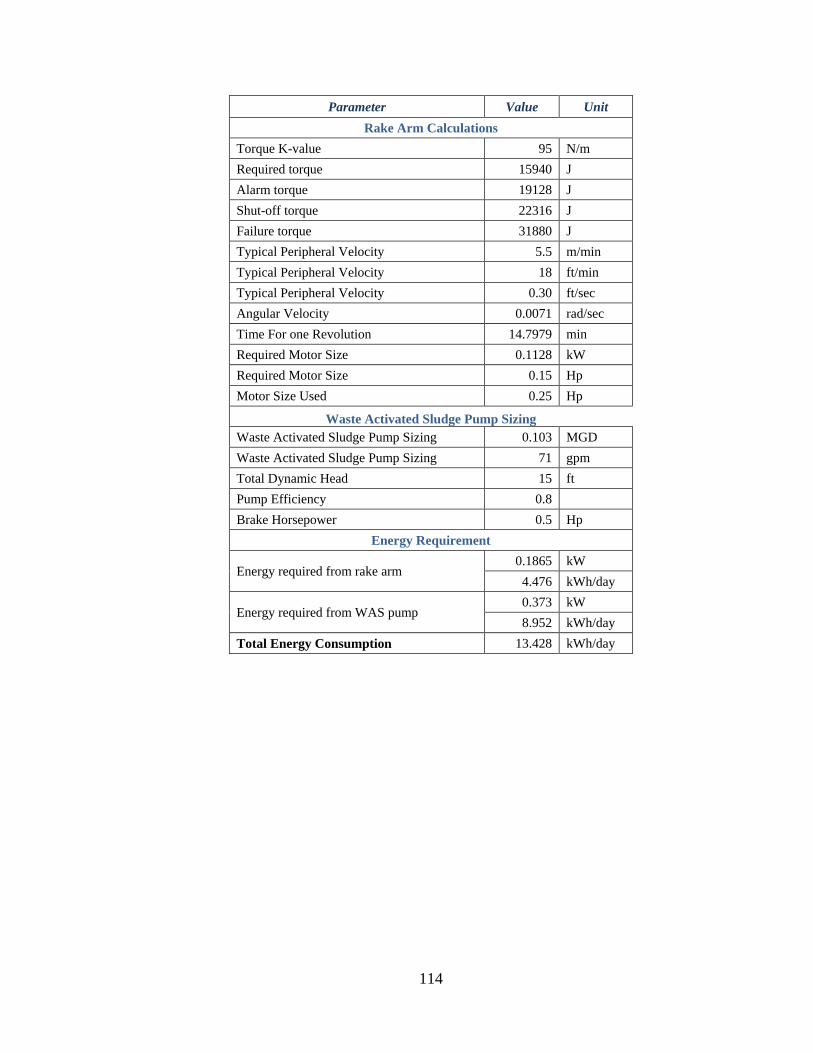
114
Parameter Value Unit
Rake Arm Calculations
Torque K-value 95 N/m
Required torque 15940 J
Alarm torque 19128 J
Shut-off torque 22316 J
Failure torque 31880 J
Typical Peripheral Velocity 5.5 m/min
Typical Peripheral Velocity 18 ft/min
Typical Peripheral Velocity 0.30 ft/sec
Angular Velocity 0.0071 rad/sec
Time For one Revolution 14.7979 min
Required Motor Size 0.1128 kW
Required Motor Size 0.15 Hp
Motor Size Used 0.25 Hp
Waste Activated Sludge Pump Sizing
Waste Activated Sludge Pump Sizing 0.103 MGD
Waste Activated Sludge Pump Sizing 71 gpm
Total Dynamic Head 15 ft
Pump Efficiency 0.8
Brake Horsepower 0.5 Hp
Energy Requirement
Energy required from rake arm 0.1865 kW
4.476 kWh/day
Energy required from WAS pump 0.373 kW
8.952 kWh/day
Total Energy Consumption 13.428 kWh/day
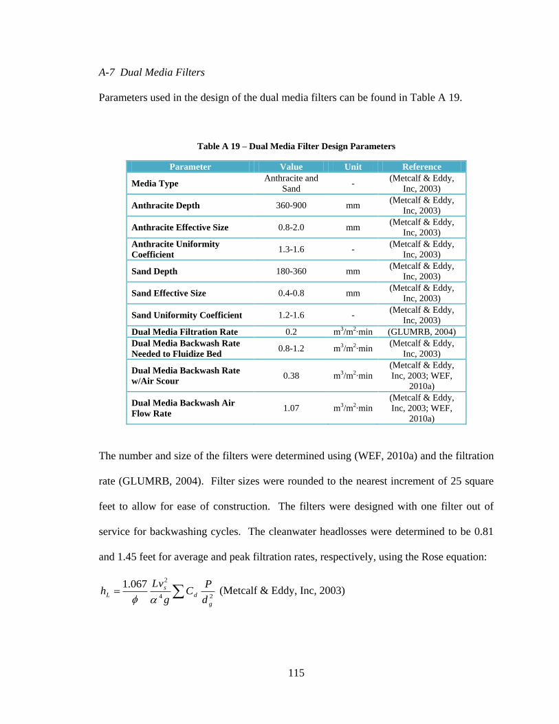
115
A-7 Dual Media Filters
Parameters used in the design of the dual media filters can be found in Table A 19.
Table A 19 – Dual Media Filter Design Parameters
Parameter Value Unit Reference
Media Type Anthracite and
Sand -
(Metcalf & Eddy,
Inc, 2003)
Anthracite Depth 360-900 mm (Metcalf & Eddy,
Inc, 2003)
Anthracite Effective Size 0.8-2.0 mm (Metcalf & Eddy,
Inc, 2003)
Anthracite Uniformity
Coefficient 1.3-1.6 -
(Metcalf & Eddy,
Inc, 2003)
Sand Depth 180-360 mm (Metcalf & Eddy,
Inc, 2003)
Sand Effective Size 0.4-0.8 mm (Metcalf & Eddy,
Inc, 2003)
Sand Uniformity Coefficient 1.2-1.6 - (Metcalf & Eddy,
Inc, 2003)
Dual Media Filtration Rate 0.2 m3/m2∙min (GLUMRB, 2004)
Dual Media Backwash Rate
Needed to Fluidize Bed 0.8-1.2 m3/m2∙min
(Metcalf & Eddy,
Inc, 2003)
Dual Media Backwash Rate
w/Air Scour 0.38 m3/m2∙min
(Metcalf & Eddy,
Inc, 2003; WEF,
2010a)
Dual Media Backwash Air
Flow Rate 1.07 m3/m2∙min
(Metcalf & Eddy,
Inc, 2003; WEF,
2010a)
The number and size of the filters were determined using (WEF, 2010a) and the filtration
rate (GLUMRB, 2004). Filter sizes were rounded to the nearest increment of 25 square
feet to allow for ease of construction. The filters were designed with one filter out of
service for backwashing cycles. The cleanwater headlosses were determined to be 0.81
and 1.45 feet for average and peak filtration rates, respectively, using the Rose equation:
24
2067.1
g
d
s
Ld
PC
g
Lvh
(Metcalf & Eddy, Inc, 2003)
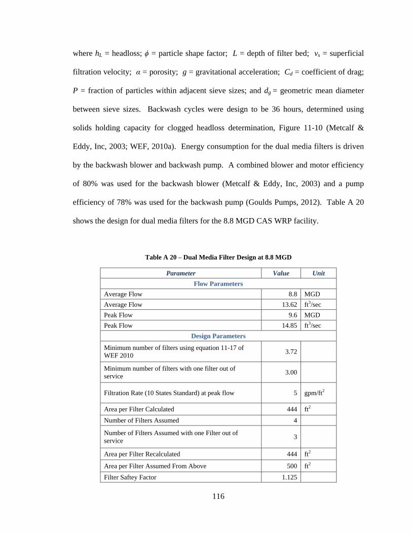
116
where hL = headloss; ϕ = particle shape factor; L = depth of filter bed; vs = superficial
filtration velocity; α = porosity; g = gravitational acceleration; Cd = coefficient of drag;
P = fraction of particles within adjacent sieve sizes; and dg = geometric mean diameter
between sieve sizes. Backwash cycles were design to be 36 hours, determined using
solids holding capacity for clogged headloss determination, Figure 11-10 (Metcalf &
Eddy, Inc, 2003; WEF, 2010a). Energy consumption for the dual media filters is driven
by the backwash blower and backwash pump. A combined blower and motor efficiency
of 80% was used for the backwash blower (Metcalf & Eddy, Inc, 2003) and a pump
efficiency of 78% was used for the backwash pump (Goulds Pumps, 2012). Table A 20
shows the design for dual media filters for the 8.8 MGD CAS WRP facility.
Table A 20 – Dual Media Filter Design at 8.8 MGD
Parameter Value Unit
Flow Parameters
Average Flow 8.8 MGD
Average Flow 13.62 ft3/sec
Peak Flow 9.6 MGD
Peak Flow 14.85 ft3/sec
Design Parameters
Minimum number of filters using equation 11-17 of
WEF 2010 3.72
Minimum number of filters with one filter out of
service 3.00
Filtration Rate (10 States Standard) at peak flow 5 gpm/ft2
Area per Filter Calculated 444 ft2
Number of Filters Assumed 4
Number of Filters Assumed with one Filter out of
service 3
Area per Filter Recalculated 444 ft2
Area per Filter Assumed From Above 500 ft2
Filter Saftey Factor 1.125
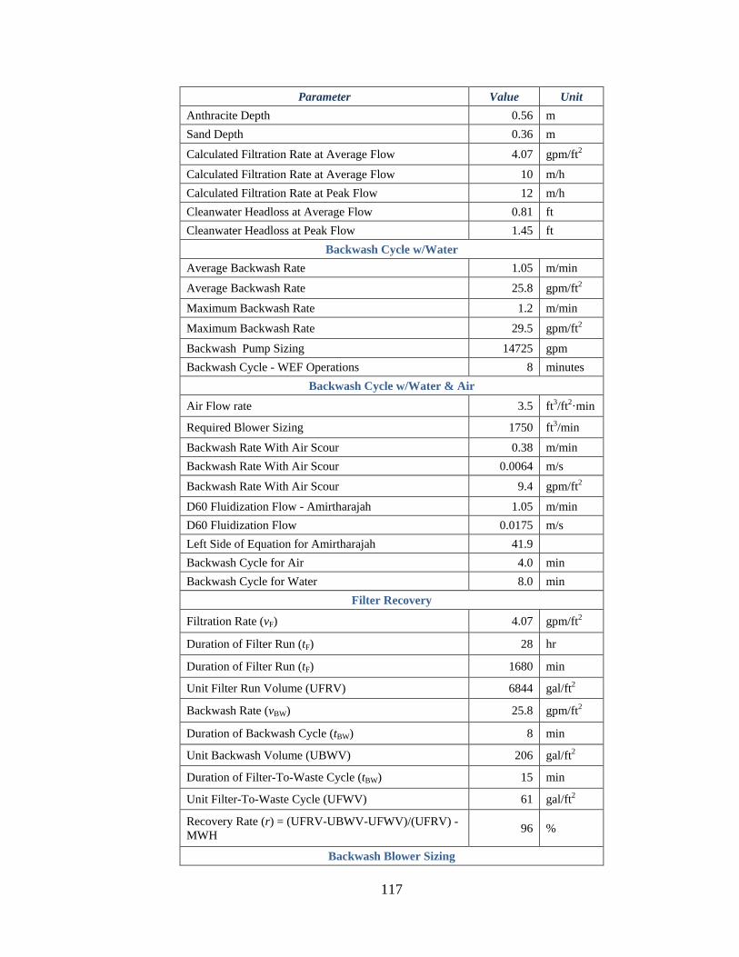
117
Parameter Value Unit
Anthracite Depth 0.56 m
Sand Depth 0.36 m
Calculated Filtration Rate at Average Flow 4.07 gpm/ft2
Calculated Filtration Rate at Average Flow 10 m/h
Calculated Filtration Rate at Peak Flow 12 m/h
Cleanwater Headloss at Average Flow 0.81 ft
Cleanwater Headloss at Peak Flow 1.45 ft
Backwash Cycle w/Water
Average Backwash Rate 1.05 m/min
Average Backwash Rate 25.8 gpm/ft2
Maximum Backwash Rate 1.2 m/min
Maximum Backwash Rate 29.5 gpm/ft2
Backwash Pump Sizing 14725 gpm
Backwash Cycle - WEF Operations 8 minutes
Backwash Cycle w/Water & Air
Air Flow rate 3.5 ft3/ft2·min
Required Blower Sizing 1750 ft3/min
Backwash Rate With Air Scour 0.38 m/min
Backwash Rate With Air Scour 0.0064 m/s
Backwash Rate With Air Scour 9.4 gpm/ft2
D60 Fluidization Flow - Amirtharajah 1.05 m/min
D60 Fluidization Flow 0.0175 m/s
Left Side of Equation for Amirtharajah 41.9
Backwash Cycle for Air 4.0 min
Backwash Cycle for Water 8.0 min
Filter Recovery
Filtration Rate (vF) 4.07 gpm/ft2
Duration of Filter Run (tF) 28 hr
Duration of Filter Run (tF) 1680 min
Unit Filter Run Volume (UFRV) 6844 gal/ft2
Backwash Rate (vBW) 25.8 gpm/ft2
Duration of Backwash Cycle (tBW) 8 min
Unit Backwash Volume (UBWV) 206 gal/ft2
Duration of Filter-To-Waste Cycle (tBW) 15 min
Unit Filter-To-Waste Cycle (UFWV) 61 gal/ft2
Recovery Rate (r) = (UFRV-UBWV-UFWV)/(UFRV) -
MWH 96 %
Backwash Blower Sizing
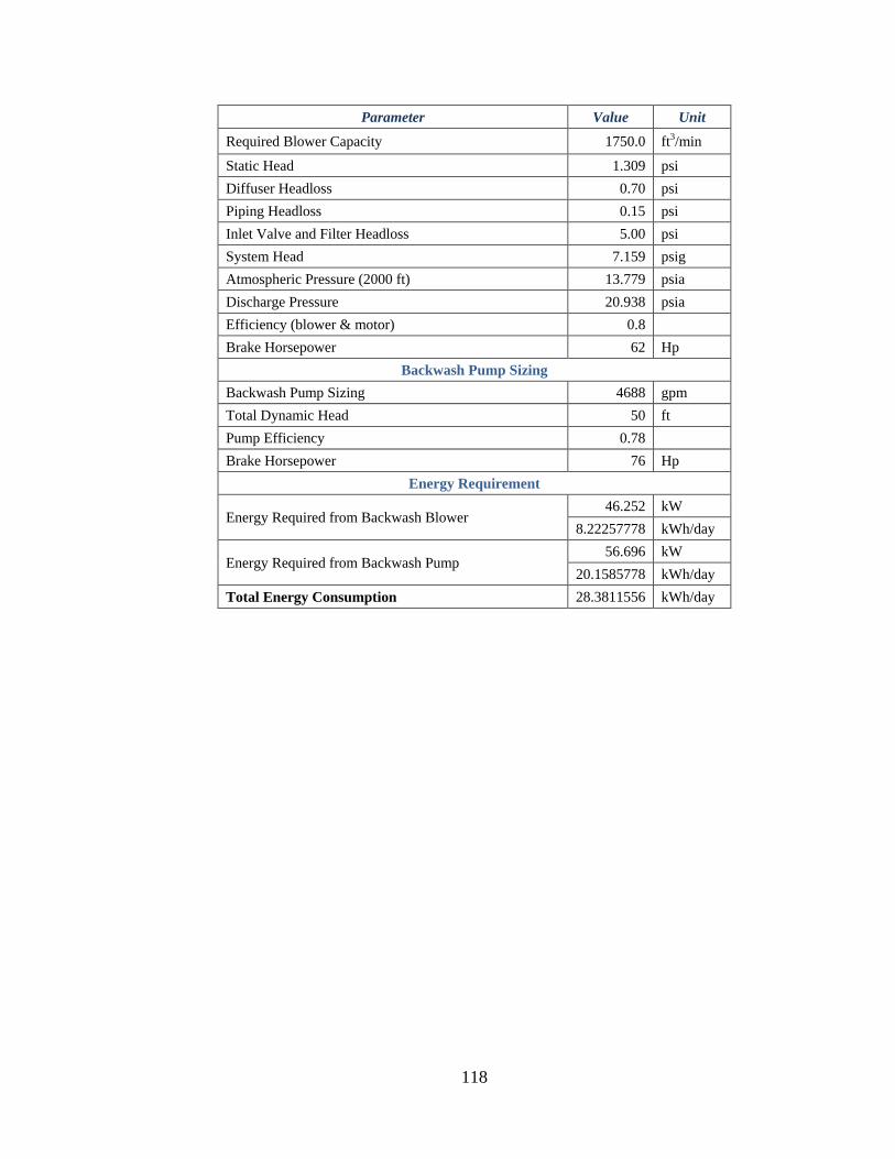
118
Parameter Value Unit
Required Blower Capacity 1750.0 ft3/min
Static Head 1.309 psi
Diffuser Headloss 0.70 psi
Piping Headloss 0.15 psi
Inlet Valve and Filter Headloss 5.00 psi
System Head 7.159 psig
Atmospheric Pressure (2000 ft) 13.779 psia
Discharge Pressure 20.938 psia
Efficiency (blower & motor) 0.8
Brake Horsepower 62 Hp
Backwash Pump Sizing
Backwash Pump Sizing 4688 gpm
Total Dynamic Head 50 ft
Pump Efficiency 0.78
Brake Horsepower 76 Hp
Energy Requirement
Energy Required from Backwash Blower 46.252 kW
8.22257778 kWh/day
Energy Required from Backwash Pump 56.696 kW
20.1585778 kWh/day
Total Energy Consumption 28.3811556 kWh/day
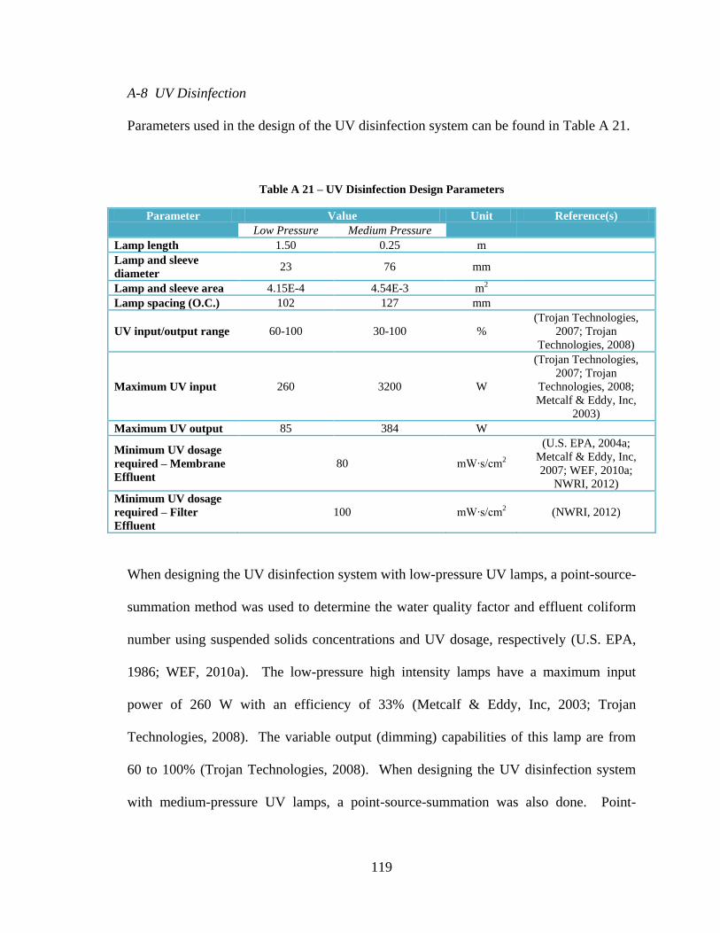
119
A-8 UV Disinfection
Parameters used in the design of the UV disinfection system can be found in Table A 21.
Table A 21 – UV Disinfection Design Parameters
Parameter Value Unit Reference(s)
Low Pressure Medium Pressure
Lamp length 1.50 0.25 m
Lamp and sleeve
diameter 23 76 mm
Lamp and sleeve area 4.15E-4 4.54E-3 m2
Lamp spacing (O.C.) 102 127 mm
UV input/output range 60-100 30-100 %
(Trojan Technologies,
2007; Trojan
Technologies, 2008)
Maximum UV input 260 3200 W
(Trojan Technologies,
2007; Trojan
Technologies, 2008;
Metcalf & Eddy, Inc,
2003)
Maximum UV output 85 384 W
Minimum UV dosage
required – Membrane
Effluent
80 mW∙s/cm2
(U.S. EPA, 2004a;
Metcalf & Eddy, Inc,
2007; WEF, 2010a;
NWRI, 2012)
Minimum UV dosage
required – Filter
Effluent
100 mW∙s/cm2 (NWRI, 2012)
When designing the UV disinfection system with low-pressure UV lamps, a point-source-
summation method was used to determine the water quality factor and effluent coliform
number using suspended solids concentrations and UV dosage, respectively (U.S. EPA,
1986; WEF, 2010a). The low-pressure high intensity lamps have a maximum input
power of 260 W with an efficiency of 33% (Metcalf & Eddy, Inc, 2003; Trojan
Technologies, 2008). The variable output (dimming) capabilities of this lamp are from
60 to 100% (Trojan Technologies, 2008). When designing the UV disinfection system
with medium-pressure UV lamps, a point-source-summation was also done. Point-

120
source-summation is a model used for estimating the UV intensity. The following
equation is used for this model
24 R
SI
(U.S. EPA, 1986)
where I = intensity at distance R; S = power available from UV source; and R =
distance of point-source. From here the UV dose can be determined by
AVGID (WEF, 2010a)
where D = Average UV dose; IAVG = array-averaged intensity from point-source-
summation; and θ = average HRT within UV light. To determine the effluent coliform
number after exposure, a variation of the Chick-Watson first-order model was developed.
The following equation is this variation
tk
OAVG
O
eNNtkIN
N /ln
(Metcalf & Eddy, Inc, 2003; U.S. EPA, 1986; Qasim,
1999; Lin, 2007; WEF, 2010a)
where N = total number of surviving disperse coliform bacteria; No = total number of
disperse coliform bacteria prior to UV light; k = inactivation rate coefficient; I = average
intensity of UV light; and t = exposure time. The medium-pressure high intensity lamps
have a maximum input power of 3,200 W with an efficiency of 12% (Metcalf & Eddy,
Inc, 2003; Trojan Technologies, 2007). The variable output capabilities of this lamp are
from 30 to 100% (Trojan Technologies, 2007). To determine the headloss through the
UV channel the following equation is used
g
vhL
28.1
2
(Metcalf & Eddy, Inc, 2003; Qasim, 1999)
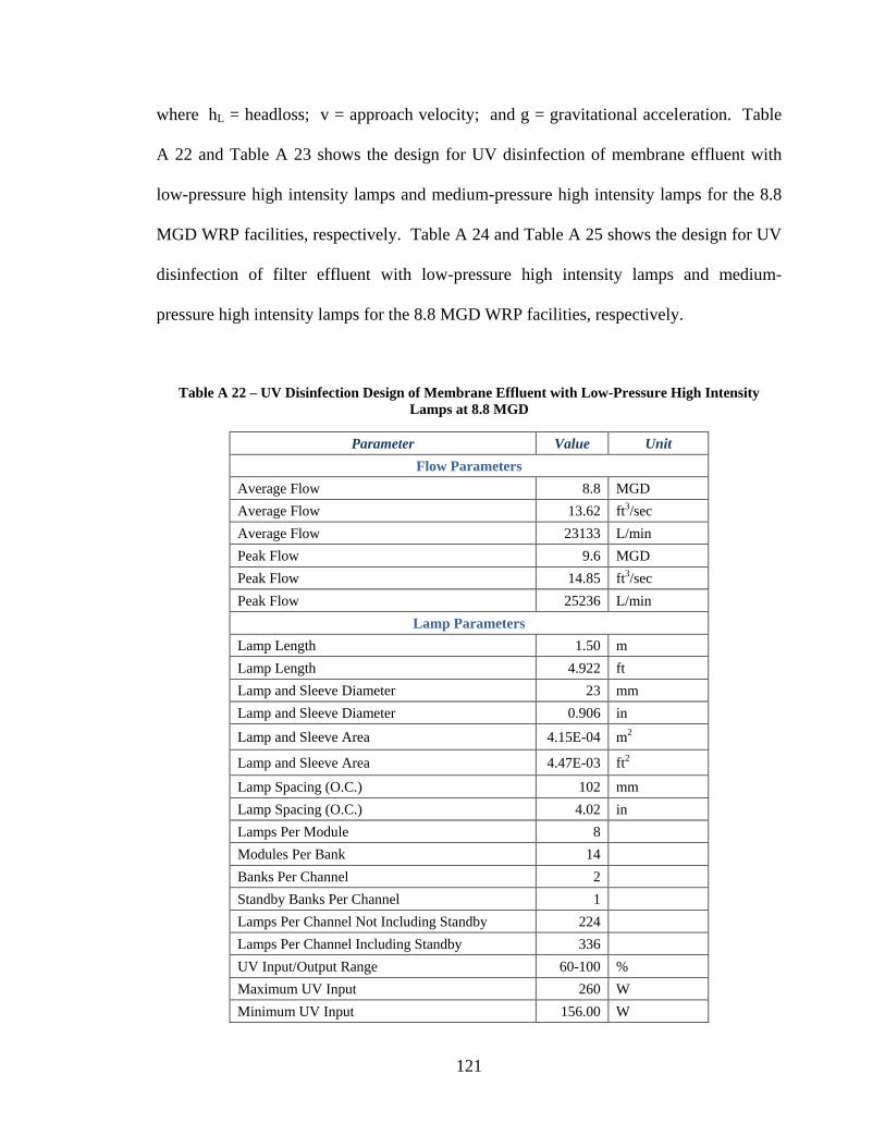
121
where hL = headloss; v = approach velocity; and g = gravitational acceleration. Table
A 22 and Table A 23 shows the design for UV disinfection of membrane effluent with
low-pressure high intensity lamps and medium-pressure high intensity lamps for the 8.8
MGD WRP facilities, respectively. Table A 24 and Table A 25 shows the design for UV
disinfection of filter effluent with low-pressure high intensity lamps and medium-
pressure high intensity lamps for the 8.8 MGD WRP facilities, respectively.
Table A 22 – UV Disinfection Design of Membrane Effluent with Low-Pressure High Intensity
Lamps at 8.8 MGD
Parameter Value Unit
Flow Parameters
Average Flow 8.8 MGD
Average Flow 13.62 ft3/sec
Average Flow 23133 L/min
Peak Flow 9.6 MGD
Peak Flow 14.85 ft3/sec
Peak Flow 25236 L/min
Lamp Parameters
Lamp Length 1.50 m
Lamp Length 4.922 ft
Lamp and Sleeve Diameter 23 mm
Lamp and Sleeve Diameter 0.906 in
Lamp and Sleeve Area 4.15E-04 m2
Lamp and Sleeve Area 4.47E-03 ft2
Lamp Spacing (O.C.) 102 mm
Lamp Spacing (O.C.) 4.02 in
Lamps Per Module 8
Modules Per Bank 14
Banks Per Channel 2
Standby Banks Per Channel 1
Lamps Per Channel Not Including Standby 224
Lamps Per Channel Including Standby 336
UV Input/Output Range 60-100 %
Maximum UV Input 260 W
Minimum UV Input 156.00 W
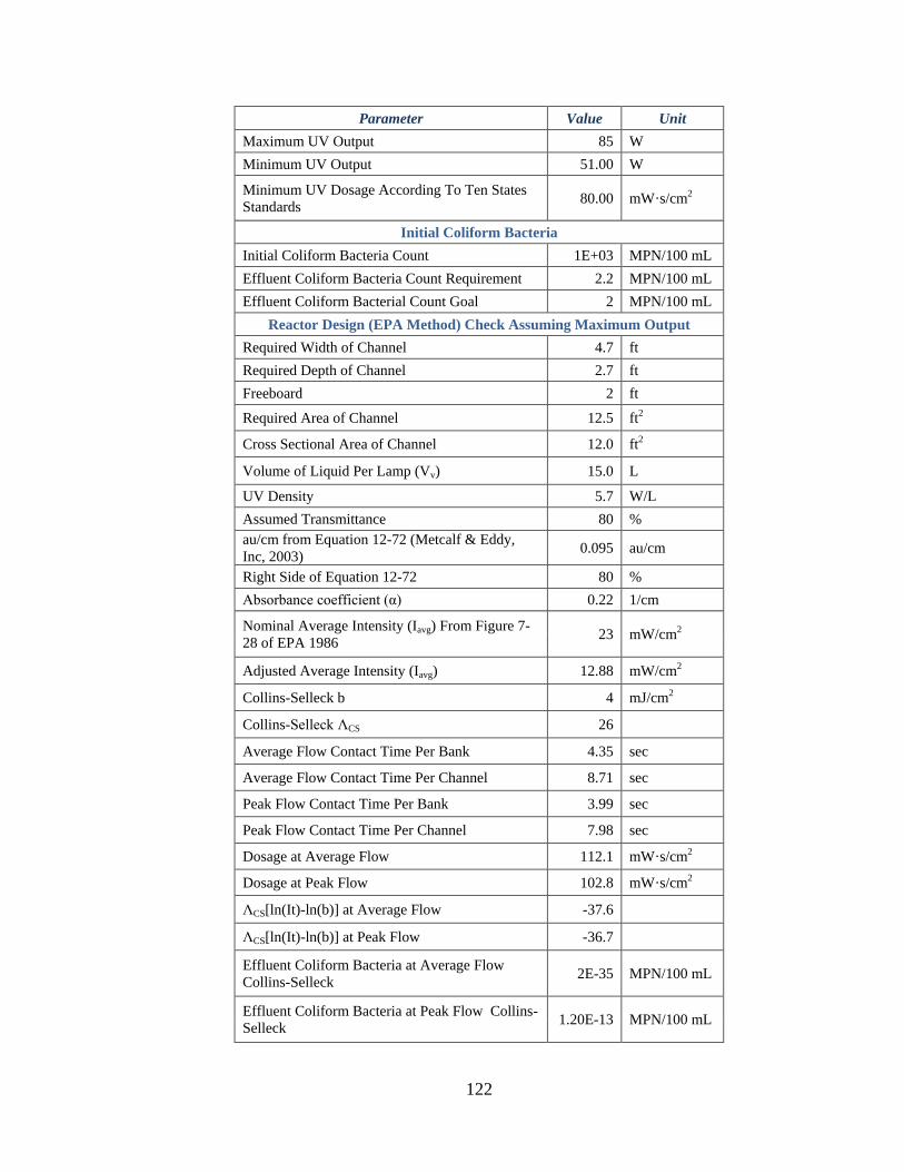
122
Parameter Value Unit
Maximum UV Output 85 W
Minimum UV Output 51.00 W
Minimum UV Dosage According To Ten States
Standards 80.00 mW·s/cm2
Initial Coliform Bacteria
Initial Coliform Bacteria Count 1E+03 MPN/100 mL
Effluent Coliform Bacteria Count Requirement 2.2 MPN/100 mL
Effluent Coliform Bacterial Count Goal 2 MPN/100 mL
Reactor Design (EPA Method) Check Assuming Maximum Output
Required Width of Channel 4.7 ft
Required Depth of Channel 2.7 ft
Freeboard 2 ft
Required Area of Channel 12.5 ft2
Cross Sectional Area of Channel 12.0 ft2
Volume of Liquid Per Lamp (Vv) 15.0 L
UV Density 5.7 W/L
Assumed Transmittance 80 %
au/cm from Equation 12-72 (Metcalf & Eddy,
Inc, 2003) 0.095 au/cm
Right Side of Equation 12-72 80 %
Absorbance coefficient (α) 0.22 1/cm
Nominal Average Intensity (Iavg) From Figure 7-
28 of EPA 1986 23 mW/cm2
Adjusted Average Intensity (Iavg) 12.88 mW/cm2
Collins-Selleck b 4 mJ/cm2
Collins-Selleck ΛCS 26
Average Flow Contact Time Per Bank 4.35 sec
Average Flow Contact Time Per Channel 8.71 sec
Peak Flow Contact Time Per Bank 3.99 sec
Peak Flow Contact Time Per Channel 7.98 sec
Dosage at Average Flow 112.1 mW·s/cm2
Dosage at Peak Flow 102.8 mW·s/cm2
ΛCS[ln(It)-ln(b)] at Average Flow -37.6
ΛCS[ln(It)-ln(b)] at Peak Flow -36.7
Effluent Coliform Bacteria at Average Flow
Collins-Selleck 2E-35 MPN/100 mL
Effluent Coliform Bacteria at Peak Flow Collins-
Selleck 1.20E-13 MPN/100 mL

123
Parameter Value Unit
E-Coli First Order Inactivation Constant From
WEF 1998 0.72 cm2/mW·s
kIavgt at average flow -80.7
kIavgt at peak flow -74.0
Effluent Coliform Bacteria at Average Flow WEF
1998 9E-33 MPN/100 mL
Effluent Coliform Bacteria at Peak Flow WEF
1998 7.27E-30 MPN/100 mL
Emerick Darby Water Quality Factor (f) From
Figure 19.36 of WEF 2010 Assuming 5 mg/L
TSS
2.00E+04
Effluent Total Coliform From Figure 19.37 of
WEF 2010 At Average Flow 2 MPN/100 mL
Effluent Total Coliform From Figure 19.37 of
WEF 2010 At Peak Flow 2 MPN/100 mL
Headloss
Velocity at Average 0.34 m/s
Velocity at Average 34.47 cm/s
Headloss at Average (Metcalf & Eddy, Inc, 2003) 0.03 m
Headloss at Average 0.11 ft
Velocity at Peak 0.38 m/s
Velocity at Peak 37.60 cm/s
Headloss at Peak (Metcalf & Eddy, Inc, 2003) 0.04 m
Headloss at Peak 0.13 ft
Average Flow Actual Dosage
UV Input Required 156 W
UV Output Required 51.0 W
Percent Illuminated 60.0 %
UV Density 3.4 W/L
Nominal Average Intensity (Iavg) From Figure 7-
28 of EPA 1986 17 mW/cm2
Adjusted Average Intensity (Iavg) 9.52 mW/cm2
Dosage at Average Flow 82.9 mW·s/cm2
ΛCS[ln(It)-ln(b)] at Average Flow -34.2
Effluent Coliform Bacteria at Average Flow
Collins-Selleck 6E-32 MPN/100 mL
kIavgt at average flow -59.67
Effluent Coliform Bacteria at Average Flow WEF
1998 1E-23 MPN/100 mL
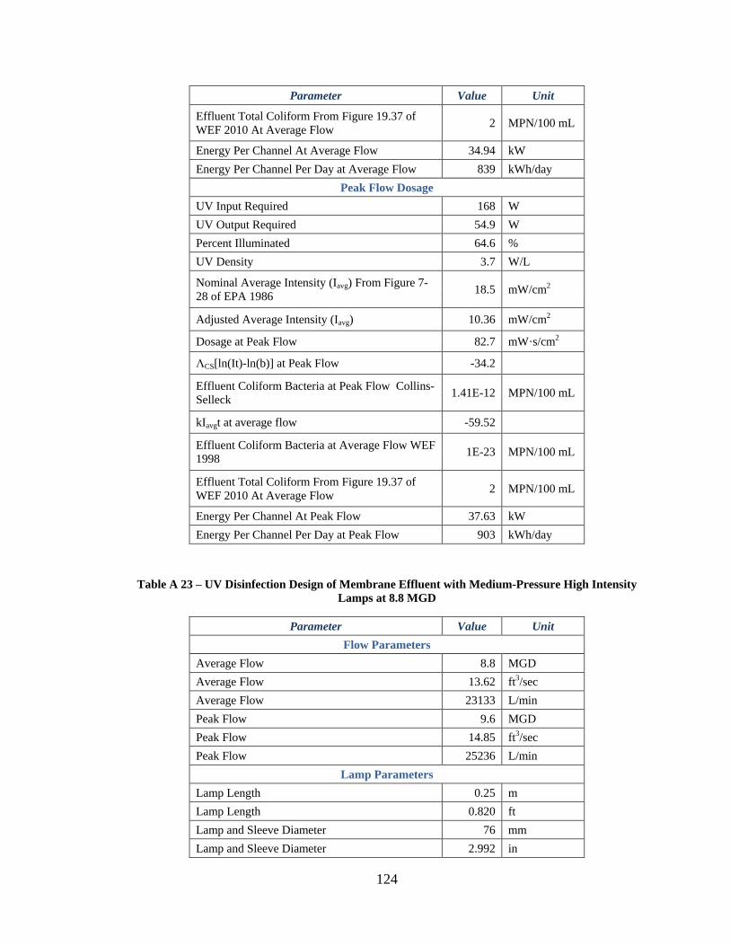
124
Parameter Value Unit
Effluent Total Coliform From Figure 19.37 of
WEF 2010 At Average Flow 2 MPN/100 mL
Energy Per Channel At Average Flow 34.94 kW
Energy Per Channel Per Day at Average Flow 839 kWh/day
Peak Flow Dosage
UV Input Required 168 W
UV Output Required 54.9 W
Percent Illuminated 64.6 %
UV Density 3.7 W/L
Nominal Average Intensity (Iavg) From Figure 7-
28 of EPA 1986 18.5 mW/cm2
Adjusted Average Intensity (Iavg) 10.36 mW/cm2
Dosage at Peak Flow 82.7 mW·s/cm2
ΛCS[ln(It)-ln(b)] at Peak Flow -34.2
Effluent Coliform Bacteria at Peak Flow Collins-
Selleck 1.41E-12 MPN/100 mL
kIavgt at average flow -59.52
Effluent Coliform Bacteria at Average Flow WEF
1998 1E-23 MPN/100 mL
Effluent Total Coliform From Figure 19.37 of
WEF 2010 At Average Flow 2 MPN/100 mL
Energy Per Channel At Peak Flow 37.63 kW
Energy Per Channel Per Day at Peak Flow 903 kWh/day
Table A 23 – UV Disinfection Design of Membrane Effluent with Medium-Pressure High Intensity
Lamps at 8.8 MGD
Parameter Value Unit
Flow Parameters
Average Flow 8.8 MGD
Average Flow 13.62 ft3/sec
Average Flow 23133 L/min
Peak Flow 9.6 MGD
Peak Flow 14.85 ft3/sec
Peak Flow 25236 L/min
Lamp Parameters
Lamp Length 0.25 m
Lamp Length 0.820 ft
Lamp and Sleeve Diameter 76 mm
Lamp and Sleeve Diameter 2.992 in

125
Parameter Value Unit
Lamp and Sleeve Area 4.54E-03 m2
Lamp and Sleeve Area 4.88E-02 ft2
Lamp Spacing (O.C.) 127 mm
Lamp Spacing (O.C.) 5.00 in
Lamps Per Module 24
Modules Per Bank 4
Banks Per Channel 1
Standby Banks Per Channel 1
Lamps Per Channel Not Including Standby 96
Lamps Per Channel Including Standby 192
UV Input/Output Range 30-100 %
Maximum UV Input 3200 W
Minimum UV Input 960.00 W
Maximum UV Output 384 W
Minimum UV Output 115.20 W
Minimum UV Dosage According To Ten States
Standards 80 mW·s/cm2
Initial Coliform Bacteria
Initial Coliform Bacteria Count 1E+03 MPN/100 mL
Effluent Coliform Bacteria Count Requirement 2.2 MPN/100 mL
Effluent Coliform Bacterial Count Goal 2 MPN/100 mL
Reactor Design (EPA Method) Check Assuming Maximum Output
Required Width of Channel 10.0 ft
Required Depth of Channel 1.7 ft
Freeboard 2 ft
Required Area of Channel 16.7 ft2
Cross Sectional Area of Channel 12.0 ft2
Volume of Liquid Per Lamp (Vv) 2.9 L
UV Density 132.5 W/L
Assumed Transmittance 80 %
au/cm from Equation 12-72 (Metcalf & Eddy,
Inc, 2003) 0.095 au/cm
Right Side of Equation 12-72 80 %
Absorbance coefficient (α) 0.22 1/cm
Nominal Average Intensity (Iavg) From PSS
Method 282.3 mW/cm2
Adjusted Average Intensity (Iavg) 158.1 mW/cm2
Collins-Selleck b 4 mJ/cm2
Collins-Selleck ΛCS 26
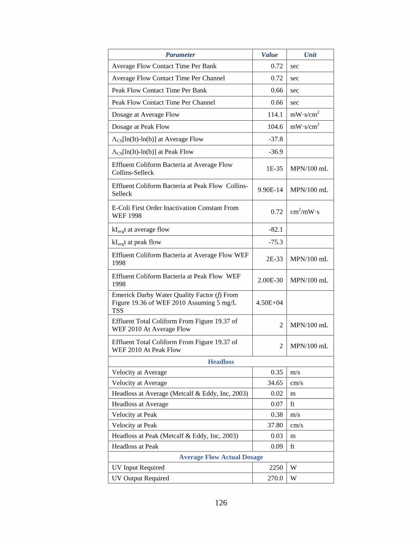
126
Parameter Value Unit
Average Flow Contact Time Per Bank 0.72 sec
Average Flow Contact Time Per Channel 0.72 sec
Peak Flow Contact Time Per Bank 0.66 sec
Peak Flow Contact Time Per Channel 0.66 sec
Dosage at Average Flow 114.1 mW·s/cm2
Dosage at Peak Flow 104.6 mW·s/cm2
ΛCS[ln(It)-ln(b)] at Average Flow -37.8
ΛCS[ln(It)-ln(b)] at Peak Flow -36.9
Effluent Coliform Bacteria at Average Flow
Collins-Selleck 1E-35 MPN/100 mL
Effluent Coliform Bacteria at Peak Flow Collins-
Selleck 9.90E-14 MPN/100 mL
E-Coli First Order Inactivation Constant From
WEF 1998 0.72 cm2/mW·s
kIavgt at average flow -82.1
kIavgt at peak flow -75.3
Effluent Coliform Bacteria at Average Flow WEF
1998 2E-33 MPN/100 mL
Effluent Coliform Bacteria at Peak Flow WEF
1998 2.00E-30 MPN/100 mL
Emerick Darby Water Quality Factor (f) From
Figure 19.36 of WEF 2010 Assuming 5 mg/L
TSS
4.50E+04
Effluent Total Coliform From Figure 19.37 of
WEF 2010 At Average Flow 2 MPN/100 mL
Effluent Total Coliform From Figure 19.37 of
WEF 2010 At Peak Flow 2 MPN/100 mL
Headloss
Velocity at Average 0.35 m/s
Velocity at Average 34.65 cm/s
Headloss at Average (Metcalf & Eddy, Inc, 2003) 0.02 m
Headloss at Average 0.07 ft
Velocity at Peak 0.38 m/s
Velocity at Peak 37.80 cm/s
Headloss at Peak (Metcalf & Eddy, Inc, 2003) 0.03 m
Headloss at Peak 0.09 ft
Average Flow Actual Dosage
UV Input Required 2250 W
UV Output Required 270.0 W
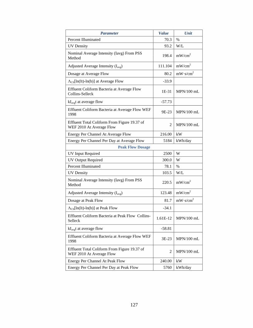
127
Parameter Value Unit
Percent Illuminated 70.3 %
UV Density 93.2 W/L
Nominal Average Intensity (Iavg) From PSS
Method 198.4 mW/cm2
Adjusted Average Intensity (Iavg) 111.104 mW/cm2
Dosage at Average Flow 80.2 mW·s/cm2
ΛCS[ln(It)-ln(b)] at Average Flow -33.9
Effluent Coliform Bacteria at Average Flow
Collins-Selleck 1E-31 MPN/100 mL
kIavgt at average flow -57.73
Effluent Coliform Bacteria at Average Flow WEF
1998 9E-23 MPN/100 mL
Effluent Total Coliform From Figure 19.37 of
WEF 2010 At Average Flow 2 MPN/100 mL
Energy Per Channel At Average Flow 216.00 kW
Energy Per Channel Per Day at Average Flow 5184 kWh/day
Peak Flow Dosage
UV Input Required 2500 W
UV Output Required 300.0 W
Percent Illuminated 78.1 %
UV Density 103.5 W/L
Nominal Average Intensity (Iavg) From PSS
Method 220.5 mW/cm2
Adjusted Average Intensity (Iavg) 123.48 mW/cm2
Dosage at Peak Flow 81.7 mW·s/cm2
ΛCS[ln(It)-ln(b)] at Peak Flow -34.1
Effluent Coliform Bacteria at Peak Flow Collins-
Selleck 1.61E-12 MPN/100 mL
kIavgt at average flow -58.81
Effluent Coliform Bacteria at Average Flow WEF
1998 3E-23 MPN/100 mL
Effluent Total Coliform From Figure 19.37 of
WEF 2010 At Average Flow 2 MPN/100 mL
Energy Per Channel At Peak Flow 240.00 kW
Energy Per Channel Per Day at Peak Flow 5760 kWh/day
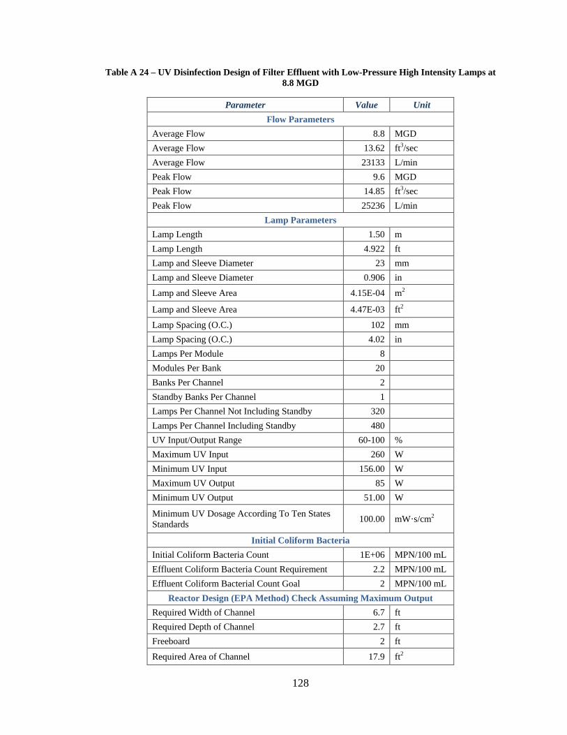
128
Table A 24 – UV Disinfection Design of Filter Effluent with Low-Pressure High Intensity Lamps at
8.8 MGD
Parameter Value Unit
Flow Parameters
Average Flow 8.8 MGD
Average Flow 13.62 ft3/sec
Average Flow 23133 L/min
Peak Flow 9.6 MGD
Peak Flow 14.85 ft3/sec
Peak Flow 25236 L/min
Lamp Parameters
Lamp Length 1.50 m
Lamp Length 4.922 ft
Lamp and Sleeve Diameter 23 mm
Lamp and Sleeve Diameter 0.906 in
Lamp and Sleeve Area 4.15E-04 m2
Lamp and Sleeve Area 4.47E-03 ft2
Lamp Spacing (O.C.) 102 mm
Lamp Spacing (O.C.) 4.02 in
Lamps Per Module 8
Modules Per Bank 20
Banks Per Channel 2
Standby Banks Per Channel 1
Lamps Per Channel Not Including Standby 320
Lamps Per Channel Including Standby 480
UV Input/Output Range 60-100 %
Maximum UV Input 260 W
Minimum UV Input 156.00 W
Maximum UV Output 85 W
Minimum UV Output 51.00 W
Minimum UV Dosage According To Ten States
Standards 100.00 mW·s/cm2
Initial Coliform Bacteria
Initial Coliform Bacteria Count 1E+06 MPN/100 mL
Effluent Coliform Bacteria Count Requirement 2.2 MPN/100 mL
Effluent Coliform Bacterial Count Goal 2 MPN/100 mL
Reactor Design (EPA Method) Check Assuming Maximum Output
Required Width of Channel 6.7 ft
Required Depth of Channel 2.7 ft
Freeboard 2 ft
Required Area of Channel 17.9 ft2
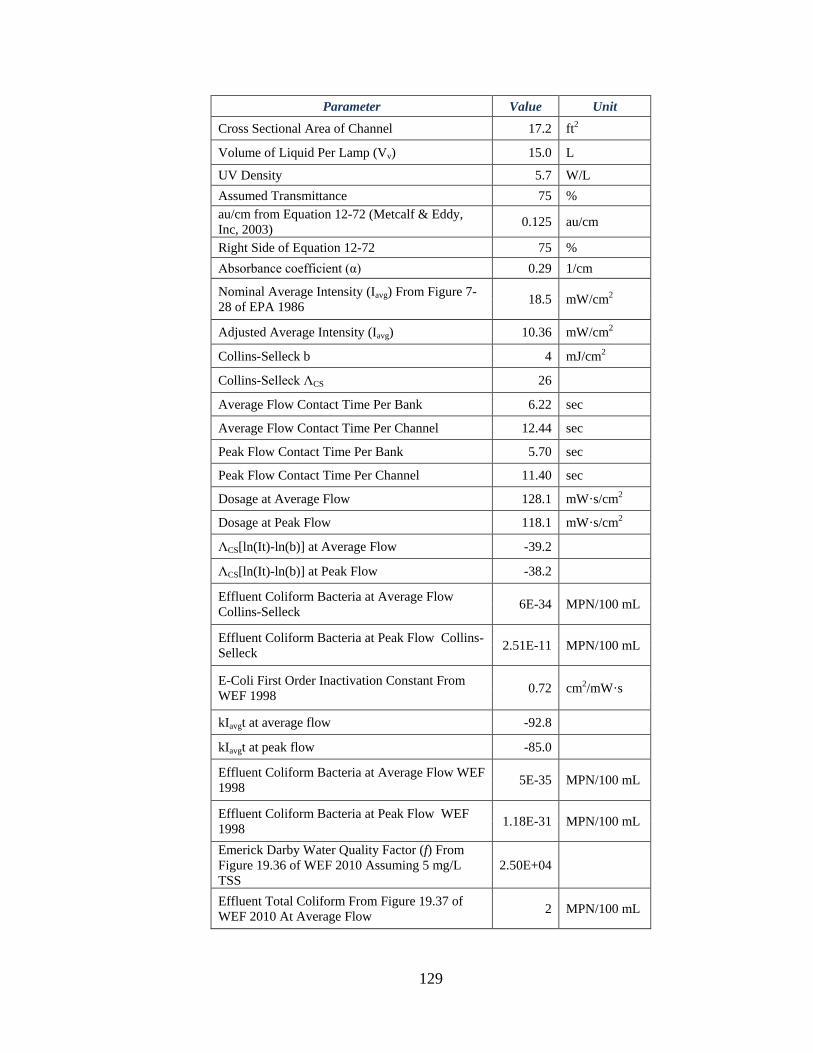
129
Parameter Value Unit
Cross Sectional Area of Channel 17.2 ft2
Volume of Liquid Per Lamp (Vv) 15.0 L
UV Density 5.7 W/L
Assumed Transmittance 75 %
au/cm from Equation 12-72 (Metcalf & Eddy,
Inc, 2003) 0.125 au/cm
Right Side of Equation 12-72 75 %
Absorbance coefficient (α) 0.29 1/cm
Nominal Average Intensity (Iavg) From Figure 7-
28 of EPA 1986 18.5 mW/cm2
Adjusted Average Intensity (Iavg) 10.36 mW/cm2
Collins-Selleck b 4 mJ/cm2
Collins-Selleck ΛCS 26
Average Flow Contact Time Per Bank 6.22 sec
Average Flow Contact Time Per Channel 12.44 sec
Peak Flow Contact Time Per Bank 5.70 sec
Peak Flow Contact Time Per Channel 11.40 sec
Dosage at Average Flow 128.1 mW·s/cm2
Dosage at Peak Flow 118.1 mW·s/cm2
ΛCS[ln(It)-ln(b)] at Average Flow -39.2
ΛCS[ln(It)-ln(b)] at Peak Flow -38.2
Effluent Coliform Bacteria at Average Flow
Collins-Selleck 6E-34 MPN/100 mL
Effluent Coliform Bacteria at Peak Flow Collins-
Selleck 2.51E-11 MPN/100 mL
E-Coli First Order Inactivation Constant From
WEF 1998 0.72 cm2/mW·s
kIavgt at average flow -92.8
kIavgt at peak flow -85.0
Effluent Coliform Bacteria at Average Flow WEF
1998 5E-35 MPN/100 mL
Effluent Coliform Bacteria at Peak Flow WEF
1998 1.18E-31 MPN/100 mL
Emerick Darby Water Quality Factor (f) From
Figure 19.36 of WEF 2010 Assuming 5 mg/L
TSS
2.50E+04
Effluent Total Coliform From Figure 19.37 of
WEF 2010 At Average Flow 2 MPN/100 mL

130
Parameter Value Unit
Effluent Total Coliform From Figure 19.37 of
WEF 2010 At Peak Flow 2 MPN/100 mL
Headloss
Velocity at Average 0.24 m/s
Velocity at Average 24.17 cm/s
Headloss at Average (Metcalf & Eddy, Inc, 2003) 0.02 m
Headloss at Average 0.05 ft
Velocity at Peak 0.26 m/s
Velocity at Peak 26.32 cm/s
Headloss at Peak (Metcalf & Eddy, Inc, 2003) 0.02 m
Headloss at Peak 0.06 ft
Average Flow Actual Dosage
UV Input Required 160 W
UV Output Required 52.3 W
Percent Illuminated 61.5 %
UV Density 3.5 W/L
Nominal Average Intensity (Iavg) From Figure 7-
28 of EPA 1986 15 mW/cm2
Adjusted Average Intensity (Iavg) 8.4 mW/cm2
Dosage at Average Flow 104.5 mW·s/cm2
ΛCS[ln(It)-ln(b)] at Average Flow -36.8
Effluent Coliform Bacteria at Average Flow
Collins-Selleck 1E-31 MPN/100 mL
kIavgt at average flow -75.21
Effluent Coliform Bacteria at Average Flow WEF
1998 2E-27 MPN/100 mL
Effluent Total Coliform From Figure 19.37 of
WEF 2010 At Average Flow 2 MPN/100 mL
Energy Per Channel At Average Flow 51.20 kW
Energy Per Channel Per Day at Average Flow 1229 kWh/day
Peak Flow Dosage
UV Input Required 190 W
UV Output Required 62.1 W
Percent Illuminated 73.1 %
UV Density 4.1 W/L
Nominal Average Intensity (Iavg) From Figure 7-
28 of EPA 1986 16.5 mW/cm2
Adjusted Average Intensity (Iavg) 9.24 mW/cm2
Dosage at Peak Flow 105.3 mW·s/cm2
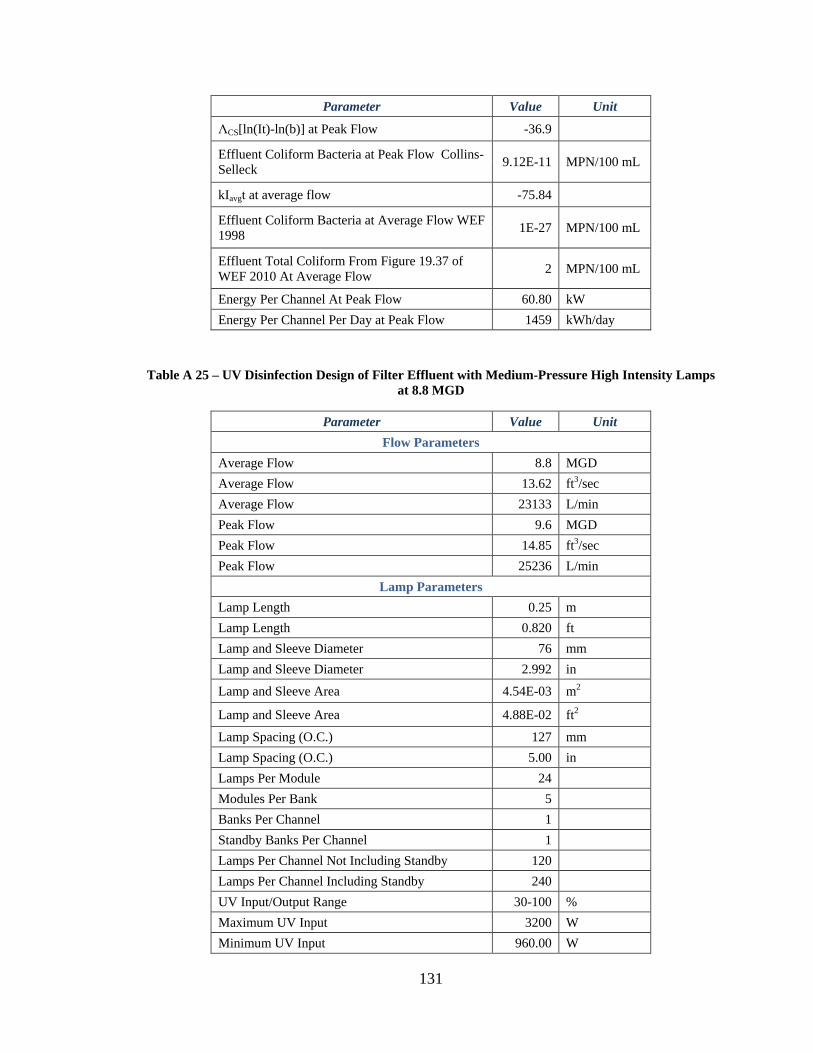
131
Parameter Value Unit
ΛCS[ln(It)-ln(b)] at Peak Flow -36.9
Effluent Coliform Bacteria at Peak Flow Collins-
Selleck 9.12E-11 MPN/100 mL
kIavgt at average flow -75.84
Effluent Coliform Bacteria at Average Flow WEF
1998 1E-27 MPN/100 mL
Effluent Total Coliform From Figure 19.37 of
WEF 2010 At Average Flow 2 MPN/100 mL
Energy Per Channel At Peak Flow 60.80 kW
Energy Per Channel Per Day at Peak Flow 1459 kWh/day
Table A 25 – UV Disinfection Design of Filter Effluent with Medium-Pressure High Intensity Lamps
at 8.8 MGD
Parameter Value Unit
Flow Parameters
Average Flow 8.8 MGD
Average Flow 13.62 ft3/sec
Average Flow 23133 L/min
Peak Flow 9.6 MGD
Peak Flow 14.85 ft3/sec
Peak Flow 25236 L/min
Lamp Parameters
Lamp Length 0.25 m
Lamp Length 0.820 ft
Lamp and Sleeve Diameter 76 mm
Lamp and Sleeve Diameter 2.992 in
Lamp and Sleeve Area 4.54E-03 m2
Lamp and Sleeve Area 4.88E-02 ft2
Lamp Spacing (O.C.) 127 mm
Lamp Spacing (O.C.) 5.00 in
Lamps Per Module 24
Modules Per Bank 5
Banks Per Channel 1
Standby Banks Per Channel 1
Lamps Per Channel Not Including Standby 120
Lamps Per Channel Including Standby 240
UV Input/Output Range 30-100 %
Maximum UV Input 3200 W
Minimum UV Input 960.00 W
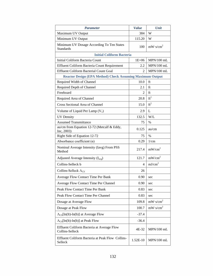
132
Parameter Value Unit
Maximum UV Output 384 W
Minimum UV Output 115.20 W
Minimum UV Dosage According To Ten States
Standards 100 mW·s/cm2
Initial Coliform Bacteria
Initial Coliform Bacteria Count 1E+06 MPN/100 mL
Effluent Coliform Bacteria Count Requirement 2.2 MPN/100 mL
Effluent Coliform Bacterial Count Goal 2 MPN/100 mL
Reactor Design (EPA Method) Check Assuming Maximum Output
Required Width of Channel 10.0 ft
Required Depth of Channel 2.1 ft
Freeboard 2 ft
Required Area of Channel 20.8 ft2
Cross Sectional Area of Channel 15.0 ft2
Volume of Liquid Per Lamp (Vv) 2.9 L
UV Density 132.5 W/L
Assumed Transmittance 75 %
au/cm from Equation 12-72 (Metcalf & Eddy,
Inc, 2003) 0.125 au/cm
Right Side of Equation 12-72 75 %
Absorbance coefficient (α) 0.29 1/cm
Nominal Average Intensity (Iavg) From PSS
Method 217.4 mW/cm2
Adjusted Average Intensity (Iavg) 121.7 mW/cm2
Collins-Selleck b 4 mJ/cm2
Collins-Selleck ΛCS 26
Average Flow Contact Time Per Bank 0.90 sec
Average Flow Contact Time Per Channel 0.90 sec
Peak Flow Contact Time Per Bank 0.83 sec
Peak Flow Contact Time Per Channel 0.83 sec
Dosage at Average Flow 109.8 mW·s/cm2
Dosage at Peak Flow 100.7 mW·s/cm2
ΛCS[ln(It)-ln(b)] at Average Flow -37.4
ΛCS[ln(It)-ln(b)] at Peak Flow -36.4
Effluent Coliform Bacteria at Average Flow
Collins-Selleck 4E-32 MPN/100 mL
Effluent Coliform Bacteria at Peak Flow Collins-
Selleck 1.52E-10 MPN/100 mL
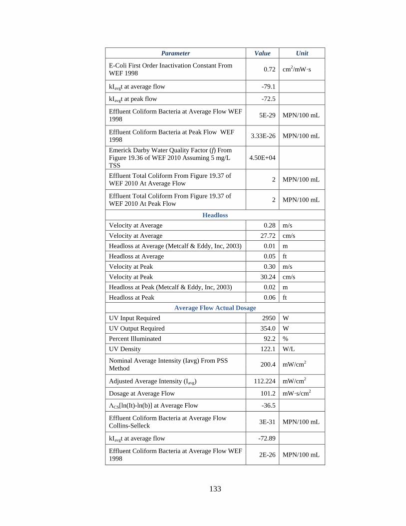
133
Parameter Value Unit
E-Coli First Order Inactivation Constant From
WEF 1998 0.72 cm2/mW·s
kIavgt at average flow -79.1
kIavgt at peak flow -72.5
Effluent Coliform Bacteria at Average Flow WEF
1998 5E-29 MPN/100 mL
Effluent Coliform Bacteria at Peak Flow WEF
1998 3.33E-26 MPN/100 mL
Emerick Darby Water Quality Factor (f) From
Figure 19.36 of WEF 2010 Assuming 5 mg/L
TSS
4.50E+04
Effluent Total Coliform From Figure 19.37 of
WEF 2010 At Average Flow 2 MPN/100 mL
Effluent Total Coliform From Figure 19.37 of
WEF 2010 At Peak Flow 2 MPN/100 mL
Headloss
Velocity at Average 0.28 m/s
Velocity at Average 27.72 cm/s
Headloss at Average (Metcalf & Eddy, Inc, 2003) 0.01 m
Headloss at Average 0.05 ft
Velocity at Peak 0.30 m/s
Velocity at Peak 30.24 cm/s
Headloss at Peak (Metcalf & Eddy, Inc, 2003) 0.02 m
Headloss at Peak 0.06 ft
Average Flow Actual Dosage
UV Input Required 2950 W
UV Output Required 354.0 W
Percent Illuminated 92.2 %
UV Density 122.1 W/L
Nominal Average Intensity (Iavg) From PSS
Method 200.4 mW/cm2
Adjusted Average Intensity (Iavg) 112.224 mW/cm2
Dosage at Average Flow 101.2 mW·s/cm2
ΛCS[ln(It)-ln(b)] at Average Flow -36.5
Effluent Coliform Bacteria at Average Flow
Collins-Selleck 3E-31 MPN/100 mL
kIavgt at average flow -72.89
Effluent Coliform Bacteria at Average Flow WEF
1998 2E-26 MPN/100 mL
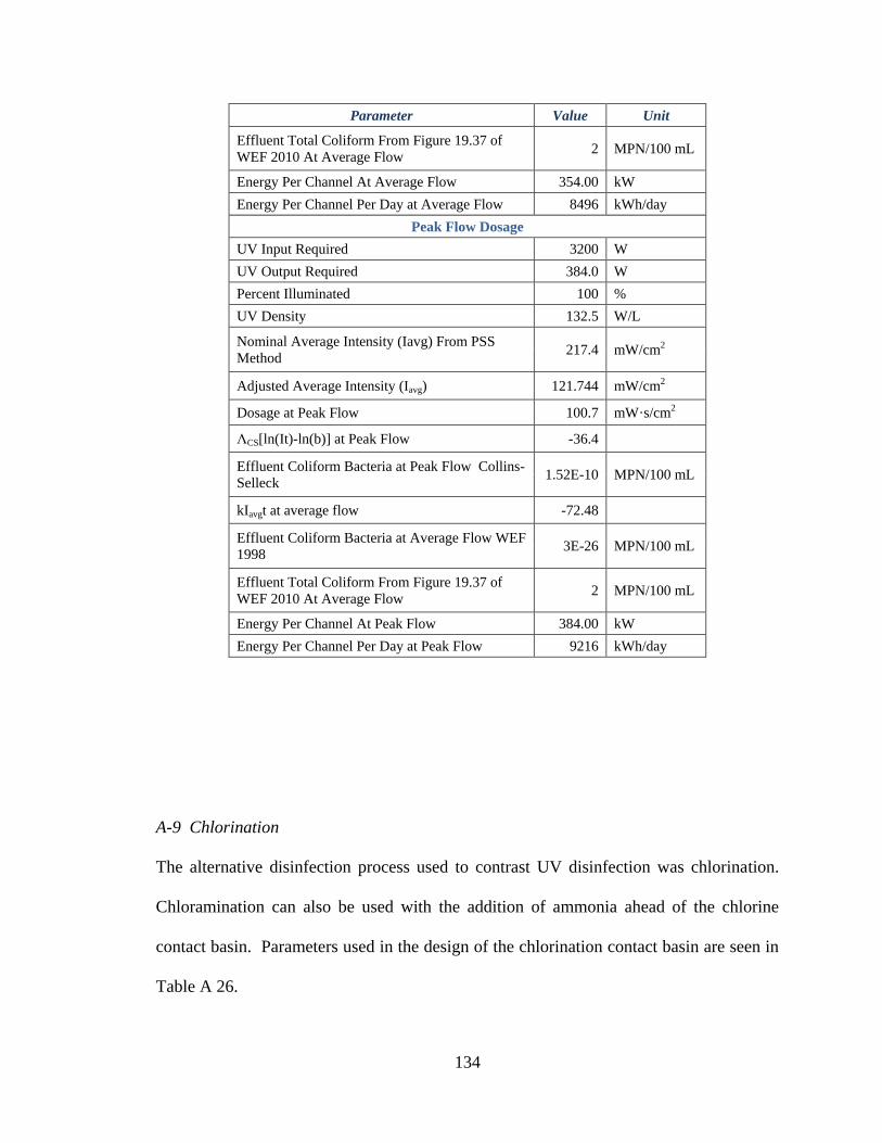
134
Parameter Value Unit
Effluent Total Coliform From Figure 19.37 of
WEF 2010 At Average Flow 2 MPN/100 mL
Energy Per Channel At Average Flow 354.00 kW
Energy Per Channel Per Day at Average Flow 8496 kWh/day
Peak Flow Dosage
UV Input Required 3200 W
UV Output Required 384.0 W
Percent Illuminated 100 %
UV Density 132.5 W/L
Nominal Average Intensity (Iavg) From PSS
Method 217.4 mW/cm2
Adjusted Average Intensity (Iavg) 121.744 mW/cm2
Dosage at Peak Flow 100.7 mW·s/cm2
ΛCS[ln(It)-ln(b)] at Peak Flow -36.4
Effluent Coliform Bacteria at Peak Flow Collins-
Selleck 1.52E-10 MPN/100 mL
kIavgt at average flow -72.48
Effluent Coliform Bacteria at Average Flow WEF
1998 3E-26 MPN/100 mL
Effluent Total Coliform From Figure 19.37 of
WEF 2010 At Average Flow 2 MPN/100 mL
Energy Per Channel At Peak Flow 384.00 kW
Energy Per Channel Per Day at Peak Flow 9216 kWh/day
A-9 Chlorination
The alternative disinfection process used to contrast UV disinfection was chlorination.
Chloramination can also be used with the addition of ammonia ahead of the chlorine
contact basin. Parameters used in the design of the chlorination contact basin are seen in
Table A 26.
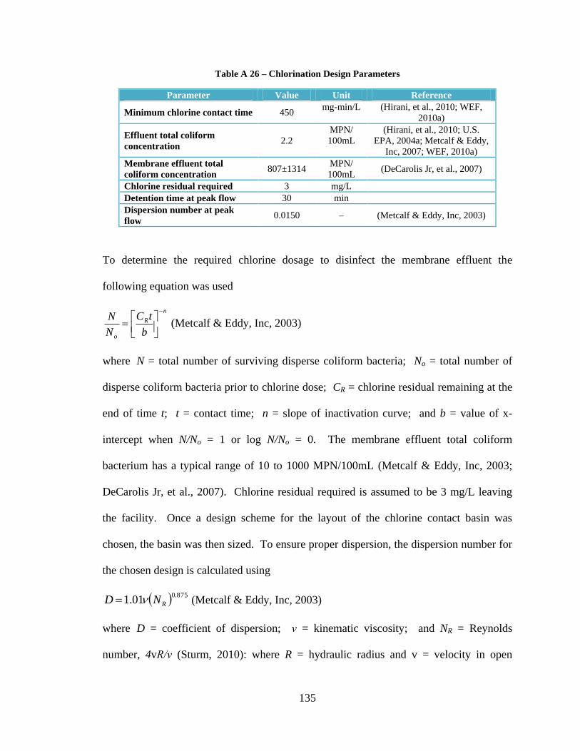
135
Table A 26 – Chlorination Design Parameters
Parameter Value Unit Reference
Minimum chlorine contact time 450 mg-min/L (Hirani, et al., 2010; WEF,
2010a)
Effluent total coliform
concentration 2.2
MPN/
100mL
(Hirani, et al., 2010; U.S.
EPA, 2004a; Metcalf & Eddy,
Inc, 2007; WEF, 2010a)
Membrane effluent total
coliform concentration 807±1314
MPN/
100mL (DeCarolis Jr, et al., 2007)
Chlorine residual required 3 mg/L
Detention time at peak flow 30 min
Dispersion number at peak
flow 0.0150 – (Metcalf & Eddy, Inc, 2003)
To determine the required chlorine dosage to disinfect the membrane effluent the
following equation was used
n
R
o b
tC
N
N
(Metcalf & Eddy, Inc, 2003)
where N = total number of surviving disperse coliform bacteria; No = total number of
disperse coliform bacteria prior to chlorine dose; CR = chlorine residual remaining at the
end of time t; t = contact time; n = slope of inactivation curve; and b = value of x-
intercept when N/No = 1 or log N/No = 0. The membrane effluent total coliform
bacterium has a typical range of 10 to 1000 MPN/100mL (Metcalf & Eddy, Inc, 2003;
DeCarolis Jr, et al., 2007). Chlorine residual required is assumed to be 3 mg/L leaving
the facility. Once a design scheme for the layout of the chlorine contact basin was
chosen, the basin was then sized. To ensure proper dispersion, the dispersion number for
the chosen design is calculated using
875.001.1 RND (Metcalf & Eddy, Inc, 2003)
where D = coefficient of dispersion; ν = kinematic viscosity; and NR = Reynolds
number, 4vR/ν (Sturm, 2010): where R = hydraulic radius and v = velocity in open
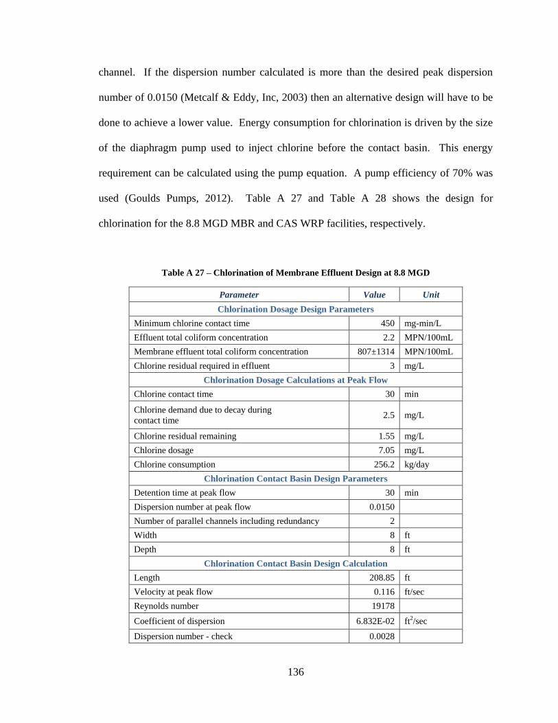
136
channel. If the dispersion number calculated is more than the desired peak dispersion
number of 0.0150 (Metcalf & Eddy, Inc, 2003) then an alternative design will have to be
done to achieve a lower value. Energy consumption for chlorination is driven by the size
of the diaphragm pump used to inject chlorine before the contact basin. This energy
requirement can be calculated using the pump equation. A pump efficiency of 70% was
used (Goulds Pumps, 2012). Table A 27 and Table A 28 shows the design for
chlorination for the 8.8 MGD MBR and CAS WRP facilities, respectively.
Table A 27 – Chlorination of Membrane Effluent Design at 8.8 MGD
Parameter Value Unit
Chlorination Dosage Design Parameters
Minimum chlorine contact time 450 mg-min/L
Effluent total coliform concentration 2.2 MPN/100mL
Membrane effluent total coliform concentration 807±1314 MPN/100mL
Chlorine residual required in effluent 3 mg/L
Chlorination Dosage Calculations at Peak Flow
Chlorine contact time 30 min
Chlorine demand due to decay during
contact time 2.5 mg/L
Chlorine residual remaining 1.55 mg/L
Chlorine dosage 7.05 mg/L
Chlorine consumption 256.2 kg/day
Chlorination Contact Basin Design Parameters
Detention time at peak flow 30 min
Dispersion number at peak flow 0.0150
Number of parallel channels including redundancy 2
Width 8 ft
Depth 8 ft
Chlorination Contact Basin Design Calculation
Length 208.85 ft
Velocity at peak flow 0.116 ft/sec
Reynolds number 19178
Coefficient of dispersion 6.832E-02 ft2/sec
Dispersion number - check 0.0028
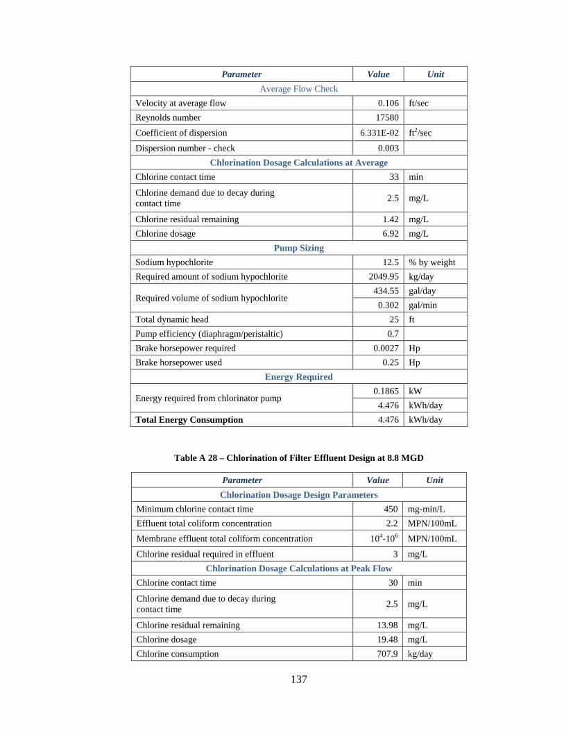
137
Parameter Value Unit
Average Flow Check
Velocity at average flow 0.106 ft/sec
Reynolds number 17580
Coefficient of dispersion 6.331E-02 ft2/sec
Dispersion number - check 0.003
Chlorination Dosage Calculations at Average
Chlorine contact time 33 min
Chlorine demand due to decay during
contact time 2.5 mg/L
Chlorine residual remaining 1.42 mg/L
Chlorine dosage 6.92 mg/L
Pump Sizing
Sodium hypochlorite 12.5 % by weight
Required amount of sodium hypochlorite 2049.95 kg/day
Required volume of sodium hypochlorite 434.55 gal/day
0.302 gal/min
Total dynamic head 25 ft
Pump efficiency (diaphragm/peristaltic) 0.7
Brake horsepower required 0.0027 Hp
Brake horsepower used 0.25 Hp
Energy Required
Energy required from chlorinator pump 0.1865 kW
4.476 kWh/day
Total Energy Consumption 4.476 kWh/day
Table A 28 – Chlorination of Filter Effluent Design at 8.8 MGD
Parameter Value Unit
Chlorination Dosage Design Parameters
Minimum chlorine contact time 450 mg-min/L
Effluent total coliform concentration 2.2 MPN/100mL
Membrane effluent total coliform concentration 104-106 MPN/100mL
Chlorine residual required in effluent 3 mg/L
Chlorination Dosage Calculations at Peak Flow
Chlorine contact time 30 min
Chlorine demand due to decay during
contact time 2.5 mg/L
Chlorine residual remaining 13.98 mg/L
Chlorine dosage 19.48 mg/L
Chlorine consumption 707.9 kg/day
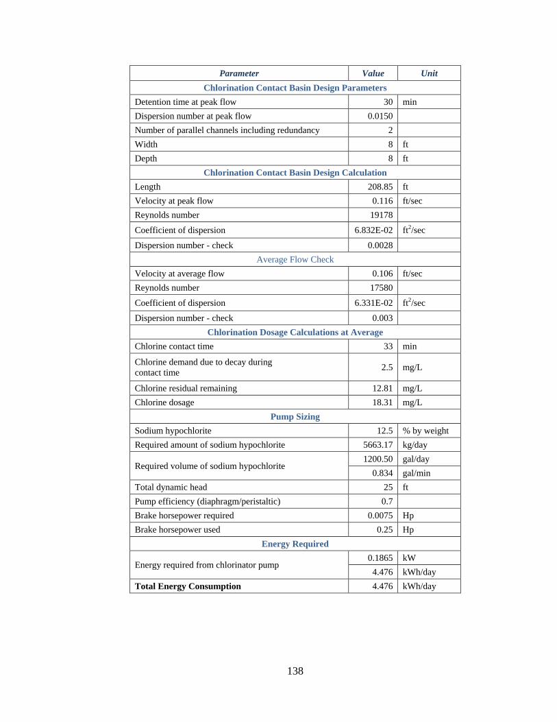
138
Parameter Value Unit
Chlorination Contact Basin Design Parameters
Detention time at peak flow 30 min
Dispersion number at peak flow 0.0150
Number of parallel channels including redundancy 2
Width 8 ft
Depth 8 ft
Chlorination Contact Basin Design Calculation
Length 208.85 ft
Velocity at peak flow 0.116 ft/sec
Reynolds number 19178
Coefficient of dispersion 6.832E-02 ft2/sec
Dispersion number - check 0.0028
Average Flow Check
Velocity at average flow 0.106 ft/sec
Reynolds number 17580
Coefficient of dispersion 6.331E-02 ft2/sec
Dispersion number - check 0.003
Chlorination Dosage Calculations at Average
Chlorine contact time 33 min
Chlorine demand due to decay during
contact time 2.5 mg/L
Chlorine residual remaining 12.81 mg/L
Chlorine dosage 18.31 mg/L
Pump Sizing
Sodium hypochlorite 12.5 % by weight
Required amount of sodium hypochlorite 5663.17 kg/day
Required volume of sodium hypochlorite 1200.50 gal/day
0.834 gal/min
Total dynamic head 25 ft
Pump efficiency (diaphragm/peristaltic) 0.7
Brake horsepower required 0.0075 Hp
Brake horsepower used 0.25 Hp
Energy Required
Energy required from chlorinator pump 0.1865 kW
4.476 kWh/day
Total Energy Consumption 4.476 kWh/day
139
A-10 Anaerobic Digester
Parameters used in the design of the single-stage high-rate mesophilic anaerobic
digester can be found in Table A 29. The HRT, equivalent to the SRT, was used in the
determination of the volume required for the digester (Metcalf & Eddy, Inc, 2003). The
amount of methane-forming volatile solids synthesized per day was determined using the
complete-mix high-rate digester equation, followed by the calculation of the volume of
methane gas using kinetic equations (Metcalf & Eddy, Inc, 2003; Davis, 2010). These
were done taking into account the volume of methane gas at the operating temperature of
35ºC. An egg-shaped digester was used in the design to provide a higher mixing
efficiency, improved homogeneous biomass, and most importantly, a smaller real estate
area in the WRP (Metcalf & Eddy, Inc, 2003; WEF, 2010b).
The anaerobic digestion process produces methane gas that can be used for energy
generation; however, digestion itself consumes energy. Energy consumption for the
anaerobic digester is driven by the mixers providing a homogeneous biomass mixture and
by the heat-exchanger providing heating for the sludge and heat losses through the
digester walls. Mixer energy requirements were determined based on the volume of the
digester, using an average energy consumption of 6.5 W/m3 (WEF, 2010b). The energy
requirement to heat the sludge was determined using (Metcalf & Eddy, Inc, 2003; Davis,
2010; WEF, 2010b):
iss TTCMq
where q = heat required, J/day; Ms = mass flow of sludge, kg/day; Cs = specific heat of
sludge, J/kg∙ºC; T = digestion temperature, ºC; and Ti = influent sludge temperature, ºC.
For purposes of this research, 4200 J/kg∙ºC was used for the specific heat of sludge
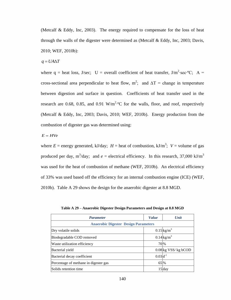
140
(Metcalf & Eddy, Inc, 2003). The energy required to compensate for the loss of heat
through the walls of the digester were determined as (Metcalf & Eddy, Inc, 2003; Davis,
2010; WEF, 2010b):
TUAq
where q = heat loss, J/sec; U = overall coefficient of heat transfer, J/m2∙sec∙ºC; A =
cross-sectional area perpendicular to heat flow, m2; and ΔT = change in temperature
between digestion and surface in question. Coefficients of heat transfer used in the
research are 0.68, 0.85, and 0.91 W/m2∙ºC for the walls, floor, and roof, respectively
(Metcalf & Eddy, Inc, 2003; Davis, 2010; WEF, 2010b). Energy production from the
combustion of digester gas was determined using:
HVeE
where E = energy generated, kJ/day; H = heat of combustion, kJ/m3; V = volume of gas
produced per day, m3/day; and e = electrical efficiency. In this research, 37,000 kJ/m
3
was used for the heat of combustion of methane (WEF, 2010b). An electrical efficiency
of 33% was used based off the efficiency for an internal combustion engine (ICE) (WEF,
2010b). Table A 29 shows the design for the anaerobic digester at 8.8 MGD.
Table A 29 – Anaerobic Digester Design Parameters and Design at 8.8 MGD
Parameter Value Unit
Anaerobic Digester Design Parameters
Dry volatile solids 0.15 kg/m3
Biodegradable COD removed 0.14 kg/m3
Waste utilization efficiency 70 %
Bacterial yield 0.08 kg VSS/ kg bCOD
Bacterial decay coefficient 0.03 d-1
Percentage of methane in digester gas 65 %
Solids retention time 15 day
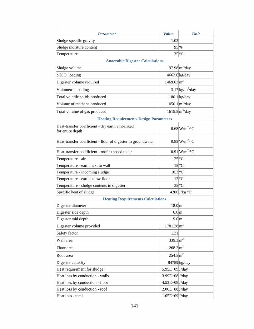
141
Parameter Value Unit
Sludge specific gravity 1.02
Sludge moisture content 95 %
Temperature 35 °C
Anaerobic Digester Calculations
Sludge volume 97.98 m3/day
bCOD loading 4663.6 kg/day
Digester volume required 1469.63 m3
Volumetric loading 3.17 kg/m3∙day
Total volatile solids produced 180.1 kg/day
Volume of methane produced 1050.1 m3/day
Total volume of gas produced 1615.5 m3/day
Heating Requirements Design Parameters
Heat-transfer coefficient - dry earth embanked
for entire depth 0.68 W/m2∙°C
Heat-transfer coefficient - floor of digester in groundwater 0.85 W/m2∙°C
Heat-transfer coefficient - roof exposed to air 0.91 W/m2∙°C
Temperature - air 25 °C
Temperature - earth next to wall 15 °C
Temperature - incoming sludge 18.3 °C
Temperature - earth below floor 12 °C
Temperature - sludge contents in digester 35 °C
Specific heat of sludge 4200 J/kg∙°C
Heating Requirements Calculations
Digester diameter 18.0 m
Digester side depth 6.0 m
Digester mid depth 9.0 m
Digester volume provided 1781.28 m3
Safety factor 1.21
Wall area 339.3 m2
Floor area 268.2 m2
Roof area 254.5 m2
Digester capacity 84789 kg/day
Heat requirement for sludge 5.95E+09 J/day
Heat loss by conduction - walls 3.99E+08 J/day
Heat loss by conduction - floor 4.53E+08 J/day
Heat loss by conduction - roof 2.00E+08 J/day
Heat loss - total 1.05E+09 J/day
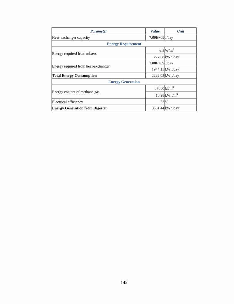
142
Parameter Value Unit
Heat-exchanger capacity 7.00E+09 J/day
Energy Requirement
Energy required from mixers 6.5 W/m3
277.88 kWh/day
Energy required from heat-exchanger 7.00E+09 J/day
1944.15 kWh/day
Total Energy Consumption 2222.03 kWh/day
Energy Generation
Energy content of methane gas 37000 kJ/m3
10.28 kWh/m3
Electrical efficiency 33 %
Energy Generation from Digester 3561.44 kWh/day

143
REFERENCES
Angelakis A and Durham B Water recycling and reuse in EUREAU countries: Trends
and challenges [Journal] // Desalination. - [s.l.] : Elsevier, 2008. - 1-3 : Vol. 218. - ISSN
00119164.
Asano T, Maeda M and Takaki M Wastewater Reclamation and Reuse in Japan:
Overview and Implementation Examples [Journal] // Water Science and Technology. -
[s.l.] : Elsevier Science Ltd, 1996. - 11 : Vol. 34. - ISSN 02731223.
ASTM International ASTM G173 - 03(2008) [Online] // Standards. - American Society
for Testing and Materials, 2012. - June 26, 2012. -
http://www.astm.org/Standards/G173.htm.
Barbose Galen [et al.] Tacking the Sun IV: An Historical Summary of the Installed Cost
of Photovoltaics in the United States from 1998 to 2010 [Report]. - [s.l.] : Environmental
Energy Technologies Division, Lawrence Berkeley National Laboratory, 2011.
Bennett Anthony Energy efficiency: Wastwater treatment and energy production
[Journal] // Filtration & Separation. - [s.l.] : Elsevier Ltd., 2007. - 10 : Vol. 44. - pp. 16-
19.
Bernier David, Osgood Jennifer and Walsh Michael Using Green to Get to Blue: How
Alternative Energy Technologies Reduce the Carbon Footprint of Wastewater Treatment
[Conference] // Water Environment Federation Technical Exhibition and Conference
2011. - Los Angeles : Water Environment Federation, 2011.
Bixio D [et al.] Wastewater reuse in Europe [Journal] // Desalination and the
Environment. - [s.l.] : Elsevier, 2006. - 1-3 : Vol. 187. - ISSN 00119164.
Brandt Malcolm [et al.] Energy efficiency in the water industry, a Global Research
Project [Journal] // Water Practice and Technology. - [s.l.] : IWA Publishing, 2011. - 2 :
Vol. 6. - ISSN 1751231X.
Burkart Christopher S and Arguea Nestor M Efficient scale for photovoltaic systems
and Florida's solar rebate program [Journal] // Energy Policy. - [s.l.] : Elsevier, 2012. -
Vol. 48.
California Energy Commission A Guide to Photovoltaic (PV) System Design and
Installation [Online]. - Callifornia Energy Commision Energy Technology Development
Division, June 2001. - June 26, 2012. -
http://www.ecodiy.org/california%20PV/californian%20photovoltaic%20best.htm.
144
City of Boulder Wastewater Treament Plant Solar Photovoltaic Facility [Online] // City
of Boulder Colorado. - January 02, 2012. - July 26, 2012. -
http://www.bouldercolorado.gov/index.php?option=com_content&task=view&id=8763&
Itemid=1189 .
Cleary Joseph G, Grey Gary M and Helmig Edward Treatment of Pharmaceuticals,
Personal Care Products and Other Microconstituents - What Technologies are Working?
[Conference] // Water Environment Federation Technical Exhibition and Conference
2011. - Los Angeles : Water Environment Federation, 2011.
Cluin Matt Effective Open Areas [E-Mail]. - [s.l.] : JWC Environmental, 2011.
Crites R and Tchobanoglous G Small and Decentralized Wastewater Management
Systems [Book]. - New York : McGraw-Hill, 1998. - ISBN 0-07-289087-8.
Crook James Water reclamation and Reuse Regulatory and Water Quality Drivers
[Conference] // Water Environment Federation Technical Exhibition and Conference
2011. - Los Angeles : Water Environment Federation, 2011.
Daigger Glen T Evolving Urban Water and Residuals Management Paradigms: Water
Reclamation and Reuse, Decentralization, and Resource Recovery [Journal] // Water
Environment Research. - [s.l.] : Water Environment Federation, 2009. - 8 : Vol. 81.
Davis Mackenzie L Water and Wastewater Engineering: Design Principles and Practice
[Book]. - New York : McGraw-Hill, 2010. - ISBN 978-0-07-171384-9.
DeCarolis James [et al.] Bottom Line - Experts Evaluate the Costs of Municipal
Membrane Bioreactors [Journal] // Water Environment & Technology. - [s.l.] : Water
Enviornment Technology, 2008. - Vol. 20.
DeCarolis Jr James F and Adham Samer Performance Investigation of Membrane
Bioreactor Systems During Municipal Wastewater Reclamation [Journal] // Water
Environment Research. - [s.l.] : Water Environment Federation, 2007. - 13 : Vol. 79. -
ISSN 10614303.
Demirbas A Global Renewable Energy Projections [Journal] // Energy Sources, Part B:
Economics, Planning, and Policy. - [s.l.] : Taylor & Francis, 2009. - 2 : Vol. 4. - ISSN
1556-7249.
Drainville Marc [et al.] Reducing the Carbon Footprint of the Hyannis WPCF Through
Renewable Energy Production and Energy Efficiency Measures [Conference] // Water
Environment Federation Technical Exhibition and Conference 2011. - Los Angeles :
Water Environment Federation, 2011.
145
Dryden Hugh and von Doenhoff A Solar Energy in the Exploration of Space
[Journal] // Proceedings of the National Academy of Sciences of the United States of
America. - [s.l.] : National Academy of Sciences, 1961. - 8 : Vol. 47.
du Pisani Petrus L Direct reclamation of potable water at Windhoek's Goreangab
reclamation plant [Journal] // Desalination. - [s.l.] : Elsevier, 2006. - 1-3 : Vol. 188. -
ISSN 00119164.
Energy Matters My Solar Estimator [Online]. - Energy Matters LLC, 2012. - June 26,
2012. - http://www.solar-estimate.org/index.php.
EPRI Program on Technology Innovation: Electric Efficiency Through Water Supply
Technologies - A Roadmap [Report]. - Palo Alto, CA : Electric Power Research Institute,
2009.
EPRI Water & Sustainability (Volume 4): U.S. Electricity Consumption for Water
Supply & Treatment - The Next Half Century [Report]. - Palo Alto, CA : Electric Power
Research Institute, 2002.
Fabiyi and E Malcolm Understanding the Alpha Factor [Journal] // Membrane
Technology. - [s.l.] : Water & Wastes Digest, 2008.
Fane A and Fane S The role of membrane technology in sustainable decentralized
watewater systems [Journal] // Water Science and Technology. - [s.l.] : IWA Publishing,
2005. - 10 : Vol. 51. - ISSN 02731223.
Find Solar Solar Calculator [Online]. - American Solar Energy Society & Cooler Planet ,
2012. - June 26, 2012. - http://www.findsolar.com/index.php?page=rightforme.
Germain E [et al.] Biomass effects on oxygen transfer in membrane bioreactors
[Journal] // Water Research. - [s.l.] : Elsevier, 2007. - Vol. 41.
GLUMRB Recommended Standards for Wastewater Facilities [Book]. - Albany, NY :
Health Research Inc., 2004.
Goodrich Alan, James Ted and Woodhouse Michael Residential, Commercial, and
Utility-Scale Photovoltaic (PV) System Prices in the United States: Current Drivers and
Cost-Reduction Opportunities [Report]. - Golden, Colorado : National Renewable Energy
Laboratory, 2012.
Goulds Pumps Pump Selection System [Java Program]. - Seneca Falls, NY : ITT
Corporation, 2012.
146
Green Martin A Radiative efficiency of state-of-the-art photovoltaic cells [Journal] //
Progress in Photovoltaics: Research and Applications. - [s.l.] : John Wiley & Sons,
2012. - Vol. 20.
Green Martin A Silicon Photovoltaic Modules: A Brief History of the First 50 Years
[Journal] // Progress in Photovoltaics: Research and Applications. - [s.l.] : John Wiley &
Sons, 2005. - Vol. 13.
Gude Verra G, Nirmalakhandan Nagamany and Deng Shuguang Renewable and
sustainable approaches for desalination [Journal] // Renewable and Sustainable Energy
Reviews. - [s.l.] : Elsevier Ltd., 2010. - Vol. 14.
Hartley Troy W Public perception and participation in water reuse [Journal] //
Desalination. - [s.l.] : Elsevier B.V., 2006. - Vol. 187. - pp. 115-126.
Hartley Troy W Water Reuse: Understanding Public Perception and Participation
[Report]. - Alexandria, Virginia : Water Environment Research Foundation, 2003.
Hecht Jeff New techniques boost photovoltaic efficiency [Journal] // Laser Focus
World. - [s.l.] : PennWell, 2010.
Hirani Zakir M [et al.] Peak flux performance and microbial removal by selected
membrane bioreactor systems [Journal] // Water Research. - [s.l.] : Elsevier Ltd, 2010. -
8 : Vol. 44. - ISSN 00431354.
Huber Technology Mechanical Wastewater Screening [Report]. - [s.l.] : Huber
Technology, 2008.
Huertas E [et al.] Key objectives for water reuse concepts [Journal] // Desalination. -
[s.l.] : Elsevier B.V., 2008. - Vol. 218. - pp. 120-131.
Ilemobade A, Adewumi J and van Zyl J Non‐Potable Water Use/Reuse in South
Africa: Review and Strategic Issues [Conference] // Water Distribution Systems Analysis
2008. - [s.l.] : American Society of Civil Engineers, 2008. - ISBN 978-0-7844-1024-0.
IRENA Renewable Energy Technologies: Cost Analysis Series - Volume 1: Power
Sector - Biomass for Power Generation [Report]. - [s.l.] : International Renewable
Energy Agency, 2012.
Jones Garr M [et al.] Pumping Station Design [Book]. - Burlington : Elsevier Inc,
2008. - ISBN 978-1-85617-513-5.
Kaya Durmus [et al.] Energy efficiency in pumps [Journal] // Energy Conversion and
Management. - [s.l.] : Elsevier, 2008. - Vol. 49.
147
Kazmi A Wastewater reclamation and reuse areas - Japanese experiences [Journal] //
Journal of Indian Water Works Association. - [s.l.] : Indian Water Works Association,
2005. - 2 : Vol. 37. - ISSN 0970275X.
Leonics How to Design Solar PV System [Online]. - Leonics Co, 2009. - June 26, 2012. -
http://www.leonics.com/support/article2_12j/articles2_12j_en.php.
Leverenz Harold L, Tchobanoglous George and Asano Takashi Direct potable reuse:
a future imperative [Journal] // Journal of Water Reuse and Desalination. - [s.l.] : IWA
Publishing, 2011. - 1 : Vol. 1.
Lin Shun D Water and Wastewater Calculations Manual [Book]. - [s.l.] : McGraw-Hill,
2007. - 2nd Edition. - ISBN 0-07-147624-5.
Liu Betty, Brumbelow Kelly and Haberl Jeff S Water/Wastewater Engineering Report
(High Efficiency Pump/Motor Replacement - M2 Model) [Report]. - [s.l.] : Texas A&M
University, 2005.
Livingston Dennis Beyond Conventional MBRs: Oxygen transfer technology
revolutionizing MBR applications [Article] // Water and Wastes Digest. - [s.l.] : Scranton
Gillette Communications, 2010. - Fall.
Mackie Alec and Oyler Kenny The Inudestry's Finest: Operators share their experiences
with the new breed of wastewater finescreens [Journal] // Water Environment &
Technology. - [s.l.] : Water Environment Federation, 2007. - 7 : Vol. 19.
Malcolm Pirnie Wastewater Treatment and Sludge Management: Energy Reference
Guide [Report]. - Albany, NY : New York State Energy Research and Development
Authority, 1995.
Mandalaki M [et al.] Assessment of fixed shading devices with integrated PV for
efficient energy use [Journal] // Solar Energy. - [s.l.] : Elsevier, 2012. - Vol. 86.
Mays Larry W Water Resources Engineering [Book]. - Hoboken, NJ : Wiley, 2010. -
2nd Edition. - ISBN 978-0-470-46064-1.
McMahon James E and Price Sarah K Water and Energy Interactions [Report] /
Annual Review of Environment and Resources. - [s.l.] : Annual Reviews, 2011.
Menniti Adrienne [et al.] The Evolution of MBR Design to Minimize Capital Cost and
Optimize Energy Efficiency [Conference] // Water Environment Federation Technical
Exhibition and Conference 2011. - Los Angeles : Water Environment Federation, 2011.

148
Messenger John [et al.] Membrane Bioreactors: Results of Low Power Use Design
Procedures [Conference] // Water Environment Federation Technical Exhibition and
Conference 2011. - Los Angeles : Water Environment Federation, 2011.
Metcalf & Eddy, Inc Wastewater Engineering: Treatment and Reuse [Book]. - New
York : Tata McGraw-Hill, 2003. - ISBN 978-0-07-049539-5.
Metcalf & Eddy, Inc Water Reuse: Issues, Technologies, and Applications [Book]. -
New York : McGraw-Hill, 2007. - ISBN 978-0-07-145927-3.
Mizuta Kentaro and Shimada Masao Benchmarking energy consumption in municipal
wastewater treatment plants in Japan [Journal] // Water Science and Technology. - [s.l.] :
IWA Publishing, 2010. - 10 : Vol. 62. - ISSN 02731223.
Navaratnasamy Mahendran, Edeogu Ike and Papworth Lawrence Economic
Feasibility of Anaerobic Digesters [Journal] // Agri-Facts. - [s.l.] : Alberta Agriculture
and Rural Development, 2008.
NRDC Water Efficiency Saves Energy: Reducing Global Warming Pollution Through
Water Use Strategies [Report]. - [s.l.] : Natural Resources Defense Council, 2009.
NREL PVWatts Grid Data Calculator (Version 2) [Online] // National Renewable
Energy Laboratory. - United States Department of Energy, June 6, 2011. - 06 26, 2012. -
http://www.nrel.gov/rredc/pvwatts/grid.html.
NWRI Ultraviolet Disinfection: Guidelines for Drinking Water and Water Reuse
[Book]. - Fountain Valley, CA : National Water Research Institute, 2012. - 3rd.
Onn Lee Water Management Issues in Singapore [Conference] // Water in Mainland
Southeast Asia. - Siem Reap, Cambodia : [s.n.], 2005.
Orange County Water District Groundwater Recharge [Online] // Groundwater
Replenishment System. - 2012. - 02 06, 2012. - http://www.gwrsystem.com/the-
process/water-delivery/groundwater-recharge.html.
Palmer Dennis W Wastewater Plant Taps Biogas, Solar and Wind [Journal] //
BioCycle. - [s.l.] : JG Press Inc, 2009. - 12 : Vol. 50.
Pellegrin Marie-Laure and Kinnear David J MBR Energy Consumption: Comparing
Operating Full-Scale Plants [Conference] // Water Environment Federation Technical
Exhibition and Conference 2011. - Los Angeles : Water Environment Federation, 2011.
Public Utilities Board NEWater [Online] // PUB, Singapore's national water agency. -
01 03, 2012. - 02 10, 2012. - http://www.pub.gov.sg/water/newater/Pages/default.aspx.
149
Qasim Syed R Wastewater Treatment Plants: Planning, Design, and Operation [Book]. -
Boca Raton : CRC Press, 1999. - ISBN 1-56676-688-5.
Rittmann Bruce E and McCarty Perry L Environmental Biotechnology: Principles and
Applications [Book]. - New York : McGraw Hill, 2001. - ISBN 0-07-234553-9.
Rosso Diego and Stenstrom Michael K Alpha Factors in Full-Scale Wastewater
Aeration Systems [Conference] // Water Environment Federation Technical Exhibition
and Conference 2006. - [s.l.] : Water Environment Federation, 2006.
Salgot M [et al.] Wastewater reuse and risk: definition of key objectives [Journal] //
Desalination. - [s.l.] : Elsevier B.V., 2006. - Vol. 187. - pp. 29-40.
Seeta Vamsi [et al.] "Free" Solar Power - A Big Leap Towards Energy Self-Sufficiency
at WWTPs [Conference] // Water Environment Federation Technical Exhibition and
Conference 2011. - Los Angeles : Water Environment Federation, 2011.
SEIA U.S. Market Installs 772 MW in Q2 2012; More than Doubling Q2 2011 Market
Size [Online] // Solar Industry Data. - Solar Energy Industries Association, 2012. -
November 20, 2012. - http://www.seia.org/research-resources/solar-industry-data.
Shrestha Eleeja [et al.] Carbon footprint of water conveyance versus desalination as
alternatives to expand water supply [Journal] // Desalination. - [s.l.] : Elsevier, 2011. - 1-
3 : Vol. 280.
Shrestha Eleeja [et al.] The carbon footprint of water management policy options
[Journal] // Energy Policy. - [s.l.] : Elsevier, 2012. - Vol. 42.
Smith & Loveless PISTA Grit Removal Systems Clears Highest Grit Removal
Efficiencies // PISTA Grit Removal System. - [s.l.] : Smith & Loveless Inc., 2007.
Sobhani Reza [et al.] Energy Footprint Analysis of Orange County Sanitation District's
Operations [Conference] // Water Environment Federation Technical Exhibition and
Conference 2011. - Los Angeles : Water Environment Federation, 2011.
Spanggaard Holger and Krebs Frederik C A brief history of the development of
organic and polymeric photovoltaics [Journal] // Solar Energy Materials & Solar Cells. -
[s.l.] : Elsevier, 2004. - Vol. 83.
Sturm Terry W Open Channel Hydraulics [Book]. - New York : McGraw-Hill, 2010. -
2nd Edition. - ISBN 978-0-07-339787-0.
Tchobanoglous G [et al.] Decentralized wastewater management: challenges and
opportunities for the twenty-first century [Journal] // Water Science and Technology:
Water Supply. - [s.l.] : IWA Publishing, 2004. - 1 : Vol. 4. - ISSN 16069749.
150
Tchobanoglous George [et al.] Direct Potable Reuse: A Path Forward [Report]. -
Washington, DC : WateReuse Research and WateReuse California, 2011.
The World Bank World Development Report 2010: Development and Climate Change
[Book]. - Washington DC : The International Bank for Reconstruction and Development
/ The World Bank, 2010. - ISBN 978-0-8213-7989-5.
Toze Simon Reuse of effluent water - benefits and risks [Journal] // Agricultural water
management. - [s.l.] : Elsevier B.V., 2006. - Vol. 80. - pp. 147-159.
Trabish Herman K The Water-Energy Nexus and Our Infrastructure Gap [Online] //
greentechmedia:. - GTM Research, February 16, 2012. - February 19, 2012. -
http://www.greentechmedia.com/articles/read/The-Water-Energy-Nexus-and-Our-
Infrastructure-Gap/.
Trojan Technologies TrojanUV3000Plus Brochure [Online] // Trojan UV. - 2008. - 03
30, 2012. -
http://trojanuv.com/resources/trojanuv/Products/TrojanUV3000Plus/TROW1040_3000Pl
us_Detailer_LR.pdf.
Trojan Technologies TrojanUV4000Plus Brochure [Online] // Trojan UV. - 2007. - 03
30, 2012. -
http://trojanuv.com/resources/trojanuv/Products/TrojanUV4000Plus/TROJANUV_4000P
lus.pdf.
U.S. EIA Electeic Power Sector Consumption Estimates [Online] // State Energy Data
System. - United States Energy Information Administration, 2010. - September 16,
2012. - http://www.eia.gov/state/seds/sep_use/total/pdf/use_NV.pdf.
U.S. EIA Electric Power Annual 2010 [Online] // Electricity. - United States Energy
Information Administration, November 9, 2011b. - July 13, 2012. -
http://www.eia.gov/electricity/annual/.
U.S. EIA World total primary energy consumption by region, Reference case, 2006-2035
[XLSX] = International Energy Outlook 2011. - [s.l.] : United States Energy Information
Administration, 2011a.
U.S. EPA Calculations and References [Online] // Clean Energy. - United States
Environmental Protection Agency, May 31, 2012. - September 18, 2012. -
http://www.epa.gov/cleanenergy/energy-resources/refs.html.
U.S. EPA Clean Watersheds Needs Survey 2004: Report to Congress [Report]. -
Washington DC : United States Environmental Protection Agency, 2004b.
151
U.S. EPA Clean Watersheds Needs Survey 2008: Report to Congress [Report]. -
Washington DC : United States Environmental Protection Agency, 2008.
U.S. EPA Ensuring a Sustainable Future: An Energy Management Guidebook for
Wastewater and Water Utilities [Report]. - Washington DC : United States
Environmental Protection Agency, 2008.
U.S. EPA Evaluation of Energy Conservation Measures for Wastewater Treatment
Facilities [Report] / Office of Wastewater Management. - Washington DC : United States
Environmental Protection Agency, 2010.
U.S. EPA Fine Pore Aeration Systems - Design Manual [Book]. - Cincinnati : United
States Environmental Protection Agency, 1989.
U.S. EPA Guidelines for Water Reuse [Report] / Office of Wastewater Management. -
Washington, DC : United States Environmental Protection Agency, 2004a.
U.S. EPA Municpal Wastewater Disinfection Design Manual [Book]. - Cincinnati :
United States Environmental Protection Agency, 1986.
U.S. EPA Nitrogen Control Manual [Book]. - Washington DC : United States
Environmental Protection Agency, 1993.
UNFCCC Kyoto Protocol [Online] // United Nations Framework Convention on Climate
Change. - 2012. - February 18, 2012. - http://unfccc.int/kyoto_protocol/items/2830.php.
Urkiaga A [et al.] Development of analysis tools for social, economic and ecological
effects of water reuse [Journal] // Desalination. - [s.l.] : Elsevier B.V., 2008. - Vol. 218. -
pp. 81-91.
URS Evaluation of Ultraviolet (UV) Radiation Disinfection Technologies for Wastewater
Treatment Plant Effluent [Report]. - Albany, NY : New York State Energy and Research
Development Authority, 2004.
Verrecht Bart [et al.] Model-based energy optimisation of a small-scale decentralised
membrane bioreactor for urban use [Journal] // Water Research. - [s.l.] : Elsevier Ltd.,
2010. - Vol. 44.
Vulcan Industries, Inc Mensch Crawler Bar Screen [Book]. - Missouri Valley, IA :
Vulcan Industries, Inc, 2011.
Wallis-Lage Cindy and Levesque Scott D Energy-efficient MBRs [Journal] // Water
Environment & Technology. - [s.l.] : Water Environment Federation, 2011.

152
WEF Clarifier Design [Book]. - New York : McGraw-Hill, 2005. - 2nd Edition. - ISBN
0-07-146416-6.
WEF Design of Municipal Wastewater Treatment Plants [Book]. - [s.l.] : McGraw-Hill,
2010a. - 5th Edition. - ISBN 978-0-07-166358-8.
WEF Energy Conservation in Water and Wastewater Facilities [Book]. - New York :
McGraw-Hill, 2010b. - ISBN 978-0-07-166794-4.
WEF Membrane Bioreactors [Book]. - New York : McGraw-Hill, 2012. - ISBN 978-0-
07-175366-1.
WEF Membrane Systems for Wastewater Treatment [Book]. - New York : McGraw-Hill,
2006. - ISBN 0-07-146419-0.
WEF Nutrient Removal [Book]. - New York : McGraw-Hill, 2011. - ISBN 978-0-07-
173709-8.
WEF Operation of Municipal Wastewater Treatment Plants [Book]. - New York :
McGraw-Hill, 2008. - ISBN 978-0071543675.
WHO WHO Guidelines for the Safe Use of Wastewater, Excreta and Greywater:
Volumes 1-4 [Report]. - Geneva, Switzerland : World Health Organization Press, 2006.
Yang Lingbo [et al.] Operational energy performance assessment system of municipal
wastewater treatment plants [Journal] // Water Science & Technology. - [s.l.] : IWA
Publishing, 2010. - 6 : Vol. 62.
Yi Lili, Chen Xiaoning and Chen Weiping An overview of reclaimed water reuse in
China [Journal] // Journal of Environmental Sciences. - [s.l.] : Chinese Academy of
Sciences, 2011. - 10 : Vol. 23. - ISSN 10010742.
153
VITA
Graduate College
University of Nevada, Las Vegas
Jonathan R Bailey
Degrees:
Bachelor of Science in Engineering, Civil Engineering, 2010
University of Nevada, Las Vegas
Publications:
Bailey, Jonathan R; Batista, Jacimaria R; Ahmad, Sajjad. Water Reuse and
Energy Interactions. Presentation at the Tri-State Seminar Annual
Conference. Primm, NV. September 25-27, 2012.
Bailey, Jonathan R. Water Reuse and Energy Interactions. Presentation at the
Nevada Water Environment Association (NWEA) Annual Conference.
Sparks, NV. April 24-25, 2012.
Newell, Timothy; Bailey, Jonathan R; Batista, Jacimaria R; Risso, LeAnna; Mills,
Jeff. Vivianite Formation Potential in Biological Phosphorus Removal
Systems. Presentation at the Nevada Water Environment Association
(NWEA) Annual Conference. Sparks, NV. April 24-25, 2012.
Bailey, Jonathan R; Newell, Timothy; Batista, Jacimaria R. Potential for Vivianite
Formation at the Solids Handling Centrifuges of the Clark County Water
Reclamation District – Technical Report. October 2011.
Thesis Title:
Investigating the Impacts of Conventional and Advanced Treatment Technologies
on Energy Consumption at Satellite Water Reuse Plants

154
Thesis Examination Committee:
Committee Co-Chair, Jacimaria R. Batista, Ph. D
Committee Co-Chair, Sajjad Ahmad, Ph. D
Committee Member, Jose Christiano Machado Jr., Ph. D
Graduate Faculty Representative, Yahia Baghzouz, Ph. D