items - the 1st workshop on user engagement optimization at
TRANSCRIPT

Recommending Items to Users: An Explore Exploit
Perspective
Deepak Agarwal, Director Machine Learning and
Relevance Science, LinkedIn, USA
CIKM, 2013

Disclaimer
Opinions expressed are mine and in no way
represent the official position of LinkedIn
Material inspired by work done at LinkedIn and
Yahoo!

Main Collaborators: several others at both Y! and
I won’t be here without them, extremely lucky to work with such
talented individuals
Bee-Chung Chen Liang Zhang Bo Long
Jonathan Traupman

Item Recommendation problem
Arises in both advertising and content
Serve the “best” items (in different
contexts) to users in an automated
fashion to optimize long-term
business objectives
Business Objectives
User engagement, Revenue,…

LinkedIn Today: Content Module
Objective: Serve content to maximize engagement
metrics like CTR (or weighted CTR)

Similar problem:
Content recommendation on Yahoo! front page
Recommend content links
(out of 30-40, editorially
programmed)
4 slots exposed, F1 has
maximum exposure
Routes traffic to other Y!
properties
F1 F2 F3 F4
Today module

LinkedIn Ads: Match ads to users visiting LinkedIn

Right Media Ad Exchange: Unified Marketplace
Match ads to page views on publisher sites
Has ad
impression
to sell --
AUCTIONS
Bids $0.50 Bids $0.75 via Network…
… which becomes
$0.45 bid
Bids $0.65—WINS!
AdSense Ad.com
Bids $0.60

High level picture
http request
Machine Learning
Models Updated in
Batch mode: e.g. once every
30 mins
Server
Item
Recommendation
system: thousands
of computations in
sub-seconds
User Interacts
e.g. click,
does nothing

High level overview: Item Recommendation System
User Info
Item Index
Id, meta-data
ML/
Statistical
Models
Score Items
P(Click), P(share),
Semantic-relevance
score,….
Rank Items:
sort by score (CTR,bid*CTR,..)
combine scores using Multi-obj optim,
Threshold on some scores,….
User-item interaction
Data: batch process
Updated in batch:
Activity, profile
Pre-filter SPAM,editorial,,..
Feature extraction
NLP, cllustering,..

ML/Statistical models for scoring
Number of items
Scored by ML Traffic volume
1000 100 100k 1M 100M
Few hours
Few days
Several days
LinkedIn Today
Yahoo! Front Page
Right Media Ad exchange
LinkedIn Ads

Explore/Exploit deployments
Yahoo! Front page Today Module (2008-2011): 300% improvement
in click-through rates
– Similar algorithms delivered via a self-serve platform, adopted by
several Yahoo! Properties (2011): Significant improvement in
engagement across Yahoo! Network
Fully deployed on LinkedIn Today Module (2012): Significant
improvement in click-through rates (numbers not revealed due to
reasons of confidentiality)
Yahoo! RightMedia exchange (2012): Fully deployed algorithms to
estimate response rates (CTR, conversion rates). Significant
improvement in revenue (numbers not revealed due to reasons of
confidentiality)
LinkedIn self-serve ads (2012): Tests on large fraction of traffic
shows significant improvements. Fully deployed.

Statistical Problem
Rank items (from an admissible pool) for user visits in
some context to maximize a utility of interest
Examples of utility functions
– Click-rates (CTR)
– Share-rates (CTR* [Share|Click] )
– Revenue per page-view = CTR*bid (more complex due to
second price auction)
CTR is a fundamental measure that opens the door to a
more principled approach to rank items
Converge rapidly to maximum utility items
– Sequential decision making process (explore/exploit)

item j from a set of candidates
User i
with
user features
(e.g., industry,
behavioral features,
Demographic
features,……)
(i, j) : response yij visits
Algorithm selects
(click or not)
Which item should we select?
The item with highest predicted CTR
An item for which we need data to
predict its CTR
Exploit
Explore
LinkedIn Today, Yahoo! Today Module:
Choose Items to maximize CTR
This is an “Explore/Exploit” Problem

The Explore/Exploit Problem (to maximize CTR)
Problem definition: Pick k items from a pool of N for a large number
of serves to maximize the number of clicks on the picked items
Easy!? Pick the items having the highest click-through rates
(CTRs)
But …
– The system is highly dynamic:
Items come and go with short lifetimes
CTR of each item may change over time
– How much traffic should be allocated to explore new items to achieve
optimal performance ?
Too little Unreliable CTR estimates due to “starvation”
Too much Little traffic to exploit the high CTR items

Y! front Page Application
Simplify: Maximize CTR on first slot (F1)
Item Pool
– Editorially selected for high quality and brand image
– Few articles in the pool but item pool dynamic

CTR Curves of Items on LinkedIn Today C
TR

Impact of repeat item views on a given user
Same user is shown an item multiple times (despite not clicking)

Simple algorithm to estimate most popular item with
small but dynamic item pool
Simple Explore/Exploit scheme
– % explore: with a small probability (e.g. 5%), choose an item at random from the pool
– (100−)% exploit: with large probability (e.g. 95%), choose highest scoring CTR item
Temporal Smoothing – Item CTRs change over time, provide more weight to recent
data in estimating item CTRs
Kalman filter, moving average
Discount item score with repeat views – CTR(item) for a given user drops with repeat views by some
“discount” factor (estimated from data)
Segmented most popular – Perform separate most-popular for each user segment

More economical exploration? Better bandit solutions
Consider two armed problem
p2 (unknown payoff
probabilities)
The gambler has 1000 plays, what is the best way to experiment ?
(to maximize total expected reward)
This is called the “multi-armed bandit” problem, have been studied for a long time.
Optimal solution: Play the arm that has maximum potential of being good
Optimism in the face of uncertainty
p1 >

Item Recommendation: Bandits?
Two Items: Item 1 CTR= 2/100 ; Item 2 CTR= 250/10000
– Greedy: Show Item 2 to all; not a good idea
– Item 1 CTR estimate noisy; item could be potentially better
Invest in Item 1 for better overall performance on average
– Exploit what is known to be good, explore what is potentially good
CTR
Pro
bab
ilit
y d
ensi
ty
Item 2
Item 1

Explore/Exploit with large item pool/personalized
recommendation
Obtaining optimal solution difficult in practice
Heuristic that is popularly used:
– Reduce dimension through a supervised learning approach
that predicts CTR using various user and item features for
“exploit” phase
– Explore by adding some randomization in an optimistic way
Widely used supervised learning approach
– Logistic Regression with smoothing, multi-hierarchy smoothing
Exploration schemes
– Epsilon-greedy, restricted epsilon-greedy, Thompson sampling, UCB

DATA
Item j with
User i
(User, context)
covariates xit
(profile information, device id,
first degree connections,
browse information,…)
item covariates Zj (keywords, content categories, ...)
(i, j) : response yij visits
Select
(click/no-click)
CONTEXT

Illustrate with Y! front Page Application
Simplify: Maximize CTR on first slot (F1)
Article Pool – Editorially selected for high quality and brand image
– Few articles in the pool but article pool dynamic
We want to provide personalized recommendations – Users with many prior visits see recommendations “tailored” to
their taste, others see the best for the “group” they belong to

Types of user covariates
Demographics, geo: – Not useful in front-page application
Browse behavior: activity on Y! network ( xit ) – Previous visits to property, search, ad views, clicks,..
– This is useful for the front-page application
Latent user factors based on previous clicks on the module ( ui )
– Useful for active module users, obtained via factor models(more later) Teases out module affinity that is not captured through other user
information, based on past user interactions with the module

Approach: Online + Offline
Offline computation
– Intensive computations done infrequently (once
a day/week) to update parameters that are less
time-sensitive
Online computation
– Lightweight computations frequent (once every 5-10
minutes) to update parameters that are time-
sensitive
– Exploration also done online

Online computation: per-item online logistic regression
For item j, the state-space model is
Item coefficients are update online via Kalman-filter

Explore/Exploit
Three schemes (all work reasonably well for the front page application)
– epsilon-greedy: Show article with maximum posterior mean except with a small probability epsilon, choose an article at random.
– Upper confidence bound (UCB): Show article with maximum score, where score = post-mean + k. post-std
– Thompson sampling: Draw a sample (v,β) from posterior to compute article CTR and show article with maximum drawn CTR

Computing the user latent factors( the u’s)
Computing user latent factors
– This is computed offline once a day using
retrospective (user,item) interaction data for last
X days (X = 30 in our case)
– Computations are done on Hadoop

Regression based Latent Factor Model
ui =Gxi +eiu, ei
u ~ N(0,diag(s1
2,s 2
2,..,s r
2 ))
vi =DZ j +e jv, e j
v ~ N(0, I)
vik ³ 0
yij ~ Ber(pij ) (# obs. per user has wide variation)
lg t(pij ) = uikv jkk
å = ¢uiv j (need shrinkage on factors)
regression weight matrix user/item-specific correction terms (learnt from data)

Role of shrinkage (consider Guassian for
simplicity)
For new user/article, factor estimates based on
covariates
For old user, factor estimates
Linear combination of prior regression function
and user feedback on items
unew =Gxnewuser, vnew =DZnew
item
E(ui | Rest) = (lI + v jv j'
jÎNi
å )-1(lGxiuser + yijv j
jÎNi
å )

Estimating the Regression function via EM
j i j
jij
i
iji
ij
ddDgGgDataf vuvuvu )),(),(),,((
Maximize
Integral cannot be computed in closed form,
approximated by Monte Carlo using Gibbs Sampling
For logistic, we use ARS (Gilks and Wild) to sample the
latent factors within the Gibbs sampler

Scaling to large data on via distributed
computing (e.g. Hadoop)
Randomly partition by users
Run separate model on each partition
– Care taken to initialize each partition model with same values, constraints on factors ensure “identifiability of parameters” within each partition
Create ensembles by using different user partitions, average across ensembles to obtain estimates of user factors and regression functions
– Estimates of user factors in ensembles uncorrelated, averaging reduces variance

Data Example
1B events, 8M users, 6K articles
Offline training produced user factor ui
Our Baseline: logistic without user feature ui
Overall click lift by including ui: 9.7%,
Heavy users (> 10 clicks last month): 26%
Cold users (not seen in the past): 3%
lgt(pijt ) = xit' b jt

Click-lift for heavy users
CTR LIFT Relative to NO ui
Logistic Model

Multiple Objectives: An example in Content
Optimization
Recommender
EDITORIAL
content Clicks on FP links influence
downstream supply distribution
AD SERVER
DISPLAY
ADVERTISING Revenue
Downstream
engagement
(Time spent)

Multiple Objectives
What do we want to optimize?
One objective: Maximize clicks
But consider the following
– Article 1: CTR=5%, utility per click = 5
– Article 2: CTR=4.9%, utility per click=10
By promoting 2, we lose 1 click/100 visits, gain 5 utils
If we do this for a large number of visits --- lose some clicks but
obtain significant gains in utility?
– E.g. lose 5% relative CTR, gain 40% in utility (e.g revenue, time spent)

An example of Multi-Objective Optimization
(Details: Agarwal et al, SIGIR 2012)
Lagrange multiplier

LinkedIn Advertising: Brand, Self-Serve, Sponsored
updates

Click Cost =
Bid3 x
CTR3/CTR2
Profile:
region = US, age = 20
Context = profile page,
300 x 250 ad slot
Ad
request
Sorted by
Bid * CTR
Response
Prediction
Engine
Campaigns eligible for
auction
Automatic
Format
Selection
Filter Campaigns
(Targeting criteria,
Frequency Cap,
Budget Pacing)
SERVING
Serving constraint < 100 millisec

CTR Prediction Model for Ads
Feature vectors
– Member feature vector: xi
– Campaign feature vector: cj
– Context feature vector: zk
Model:

CTR Prediction Model for Ads
Feature vectors
– Member feature vector: xi
– Campaign feature vector: cj
– Context feature vector: zk
Model:
Cold-start component
Warm-start
per-campaign component

CTR Prediction Model for Ads
Feature vectors
– Member feature vector: xi
– Campaign feature vector: cj
– Context feature vector: zk
Model:
Cold-start component
Warm-start
per-campaign component
Cold-start:
Warm-start:
Both can have L2
penalties.

Model Fitting
Single machine (well understood)
– conjugate gradient
– L-BFGS
– Trusted region
– …
Model Training with Large scale data
– Cold-start component Θw is more stable
Weekly/bi-weekly training good enough
However: difficulty from need for large-scale logistic regression
– Warm-start per-campaign model Θc is more dynamic
New items can get generated any time
Big loss if opportunities missed
Need to update the warm-start component as frequently as possible
Large Scale Logistic
Regression
Per-item logistic regression
given Θc

Large Scale Logistic Regression: Computational
Challenge
Hundreds of millions/billions of observations
Hundreds of thousands/millions of covariates
Fitting a logistic regression model on a single machine not feasible
Model fitting iterative using methods like gradient descent,
Newton’s method etc
– Multiple passes over the data
Problem: Find x to min(F(x))
Iteration n: xn = xn-1 – bn-1 F’(xn-1)
bn-1 is the step size that can change every iteration
Iterate until convergence
Conjugate gradient, LBFGS, Newton trust region, …
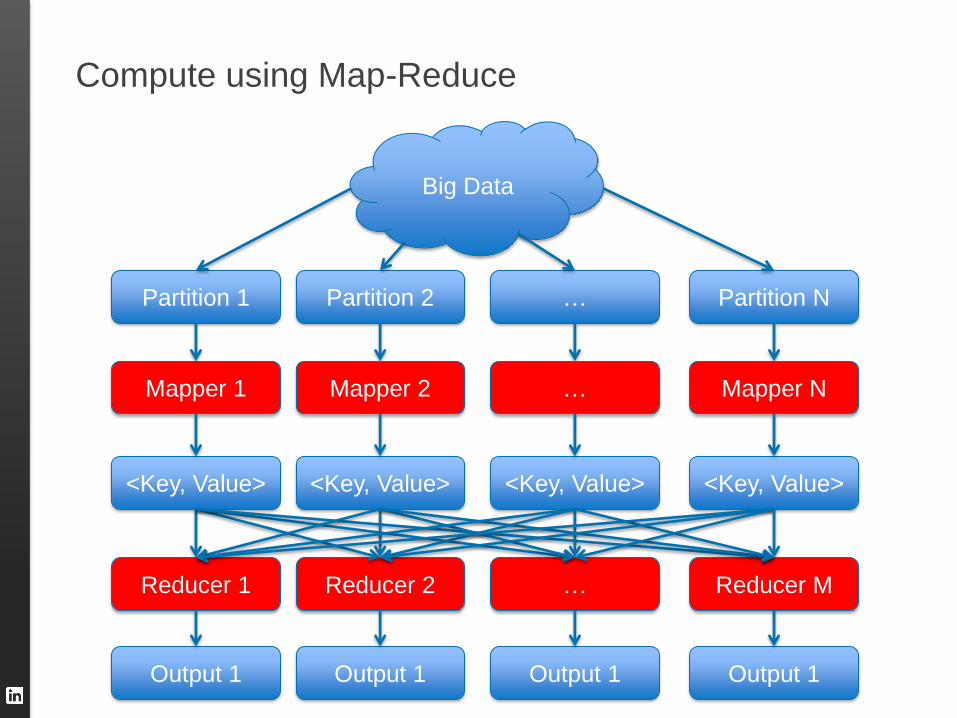
Compute using Map-Reduce
Big Data
Partition 1 Partition 2 … Partition N
Mapper 1 Mapper 2 … Mapper N
<Key, Value> <Key, Value> <Key, Value> <Key, Value>
Reducer 1 Reducer 2 Reducer M …
Output 1 Output 1 Output 1 Output 1

Large Scale Logistic Regression
Naïve:
– Partition the data and run logistic regression for each partition
– Take the mean of the learned coefficients
– Problem: Not guaranteed to converge to global solution
Alternating Direction Method of Multipliers (ADMM)
– Boyd et al. 2011
– Set up constraints: each partition’s coefficient = global consensus
– Solve the optimization problem using Lagrange Multipliers
– Advantage: converges to global solution

Large Scale Logistic Regression via ADMM
BIG DATA
Partition 1 Partition 2 Partition 3 Partition K
Logistic
Regression
Logistic
Regression Logistic
Regression
Logistic
Regression
Consensus
Computation
Iteration 1

Large Scale Logistic Regression via ADMM
BIG DATA
Partition 1 Partition 2 Partition 3 Partition K
Logistic
Regression
Consensus
Computation
Logistic
Regression
Logistic
Regression
Logistic
Regression
Iteration 1

Large Scale Logistic Regression via ADMM
BIG DATA
Partition 1 Partition 2 Partition 3 Partition K
Logistic
Regression
Logistic
Regression Logistic
Regression
Logistic
Regression
Consensus
Computation
Iteration 2

Large Scale Logistic Regression via ADMM
Notation
– (Xi , yi): data in the ith partition
– βi: coefficient vector for partition i
– β: Consensus coefficient vector
– r(β): penalty component such as ||β||22
Optimization problem

ADMM updates
LOCAL REGRESSIONS
Shrinkage towards current
best global estimate
UPDATED
CONSENSUS

ADMM at LinkedIn
Lessons and Improvements
– Initialization is important (ADMM-M)
Use the mean of the partitions’ coefficients
Reduces number of iterations by 50%
– Adaptive step size (learning rate) (ADMM-MA)
Exponential decay of learning rate
– Together, these optimizations reduce training time from 10h to 2h

Explore/Exploit with Logistic Regression
55
+ +
+ +
+
+
+
_
_
_
_
_
_
_
_
_
_ _
_
_
COLD START
COLD + WARM START
for an Ad-id
POSTERIOR of WARM-START
COEFFICIENTS
E/E: Sample a line from the
posterior
(Thompson Sampling)

Models Considered
CONTROL: per-campaign CTR counting model
COLD-ONLY: only cold-start component
LASER: our model (cold-start + warm-start)
LASER-EE: our model with Explore-Exploit using Thompson
sampling

Metrics
Model metrics
– Test Log-likelihood
– AUC/ROC
– Observed/Expected ratio
Business metrics (Online A/B Test)
– CTR
– CPM (Revenue per impression)

Observed / Expected Ratio
Observed: #Clicks in the data
Expected: Sum of predicted CTR for all impressions
Not a “standard” classifier metric, but in many ways more useful for
this application
What we usually see: Observed / Expected < 1
– Quantifies the “winner’s curse” aka selection bias in auctions
When choosing from among thousands of candidates, an item with
mistakenly over-estimated CTR may end up winning the auction
Particularly helpful in spotting inefficiencies by segment
– E.g. by bid, number of impressions in training (warmness), geo, etc.
– Allows us to see where the model might be giving too much weight to
the wrong campaigns
High correlation between O/E ratio and model performance online

Offline: ROC Curves
False Positive Rate
Tru
e P
ositiv
e R
ate
0.0
0.2
0.4
0.6
0.8
1.0
0.0
0.2
0.4
0.6
0.8
1.0
●●●●●●●●●
●●
●●
●
●
●
●
●
●
●
●
●
●●●●●●●●
●●
●●
●
●
●
●
●
●
●
●
●
●
●
●
CONTROL [ 0.672 ]COLD−ONLY [ 0.757 ]LASER [ 0.778 ]

Online A/B Test
Three models
– CONTROL (10%)
– LASER (85%)
– LASER-EE (5%)
Segmented Analysis
– 8 segments by campaign warmness
Degree of warmness: the number of training samples available in the
training data for the campaign
Segment #1: Campaigns with almost no data in training
Segment #8: Campaigns that are served most heavily in the previous
batches so that their CTR estimate can be quite accurate

Daily CTR Lift Over Control
Pe
rcenta
ge o
f C
TR
Lift
+%
+%
+%
+%
+%
Day 1
Day 2
Day 3
Day 4
Day 5
Day 6
Day 7
●
● ●
●
●
●
●●
LASERLASER−EE

Daily CPM Lift Over Control
Perc
en
tage o
f eC
PM
L
ift
+%
+%
+%
+%
+%
+%
Day 1
Day 2
Day 3
Day 4
Day 5
Day 6
Day 7
●
●
●
● ●
●
●
●
LASERLASER−EE

CPM Lift By Campaign
Warmness Segments
Campaign Warmness Segment
Lift P
erc
en
tag
e o
f C
PM
−%
−%
−%
0%
+%
+%
1 2 3 4 5 6 7 8
LASER
LASER−EE

O/E Ratio By Campaign
Warmness Segments
Campaign Warmness Segment
Obse
rved
Clic
k/E
xpe
cte
d C
licks
0.5
0.6
0.7
0.8
0.9
1
1 2 3 4 5 6 7 8
CONTROL
LASER
LASER−EE

Number of Campaigns Served Improvement from E/E

Insights
Overall performance:
– LASER and LASER-EE are both much better than control
– LASER and LASER-EE performance are very similar
Segmented analysis by campaign warmness
– Segment #1 (very cold)
LASER-EE much worse than LASER due to its exploration property
LASER much better than CONTROL due to cold-start features
– Segments #3 - #5
LASER-EE significantly better than LASER
Winner’s curse hit LASER
– Segment #6 - #8 (very warm)
LASER-EE and LASER are equivalent
Number of campaigns served
– LASER-EE serves significantly more campaigns than LASER
– Provides healthier market place

Takeaways
Reducing dimension through logistic regression coupled with
explore/exploit schemes like Thompson sampling effective
mechanism to solve response prediction problems in advertising
Partitioning model components by cold-start (stable) and warm-start
(non-stationary) with different training frequencies effective
mechanism to scale computations
ADMM with few modifications effective model training strategy for
large data with high dimensionality
Methods work well for LinkedIn advertising, significant
improvements
©2013 LinkedIn Corporation. All Rights Reserved.

Current Work
Investigating Spark and various other fitting algorithms
– Promising results, ADMM still looks good on our datasets
Stream Ads
– Multi-response prediction (clicks, shares, likes, comments)
– Filtering low quality ads extremely important
Revenue/Engagement tradeoffs (Pareto optimal solutions)
Stream Recommendation
– Holistic solution to both content and ads on the stream
Large scale ML infrastructure at LinkedIn
– Powers several recommendation systems
©2013 LinkedIn Corporation. All Rights Reserved.

Summary
Large scale Machine Learning plays an important role in recommender problems
Several such problems can be cast as explore/exploit tradeoff
Estimating interactions in high-dimensional sparse data via supervised learning important for efficient exploration and exploitation
Scaling such models to Big Data is a challenging statistical problem
Combining offline + online modeling with classical explore/exploit algorithm is a good practical strategy

Other challenges
3Ms: Multi-response, Multi-context modeling to optimize Multiple
Objectives
– Multi-response: Clicks, share, comments, likes,.. (preliminary work at
CIKM 2012)
– Multi-context: Mobile, Desktop, Email,..(preliminary work at SIGKDD
2011)
– Multi-objective: Tradeoff in engagement, revenue, viral activities
Preliminary work at SIGIR 2012, SIGKDD 2011
Scaling model computations at run-time to avoid latency issues
– Predictive Indexing (preliminary work at WSDM 2012)

Backup slides
©2013 LinkedIn Corporation. All Rights Reserved.

LASER Configuration
Feature processing pipeline – Sources: transform external data into feature vectors
– Transformers: modify/combine feature vectors
– Assembler: Packages features vectors for training/inference
Configuration language – Model structure can be changed extensively
– Library of reusable components
– Train, test, and deploy models without any code changes
– Speeds up model development cycle

LASER Transformer Pipeline
User Source Context
Source Item Source
Subset Subset
Interaction
Assembler
Request User
profile Item
Training or
Inference

LASER Performance
Real time inference
– About 10µs per inference (1500 ads = 15ms)
– Reacts to changing features immediately
“Better wrong than late”
– If a feature isn’t immediately available, back off to prior value
Asynchronous computation
– Actions that block or take time run in background threads
Lazy evaluation
– Sources & transformers do not create feature vectors for all items
– Feature vectors are constructed/transformed only when needed
Partial results cache
– Logistic regression inference is a series of dot products
– Scalars are small; cache can be huge
– Hardware-like implementation to minimize locking and heap pressure

Summary
Large scale Machine Learning plays an important role in computational advertising and content recommendation
Several such problems can be cast as explore/exploit tradeoff
Estimating interactions in high-dimensional sparse data via supervised learning important for efficient exploration and exploitation
Scaling such models to Big Data is a challenging statistical problem
Combining offline + online modeling with classical explore/exploit algorithm is a good practical strategy

Other challenges
3Ms: Multi-response, Multi-context modeling to optimize Multiple
Objectives
– Multi-response: Clicks, share, comments, likes,.. (preliminary work at
CIKM 2012)
– Multi-context: Mobile, Desktop, Email,..(preliminary work at SIGKDD
2011)
– Multi-objective: Tradeoff in engagement, revenue, viral activities
Preliminary work at SIGIR 2012, SIGKDD 2011
Scaling model computations at run-time to avoid latency issues
– Predictive Indexing (preliminary work at WSDM 2012)