jan purczyński, kamila...

Jan Purczyński, KamilaBednarz-Okrzyńska

Application of generalized student’st-distribution in modeling thedistribution of empirical return rateson selected stock exchange indexesFolia Oeconomica Stetinensia 13(21)/2, 37-48

2013

APPLICATION OF GENERALIZED STUDENT’S T-DISTRIBUTION IN MODELING THE DISTRIBUTION OF EMPIRICAL RETURN RATES

ON SELECTED STOCK EXCHANGE INDEXES

Prof. Jan Purczyński

Szczecin UniversityFaculty of Management and Economics of ServicesDepartment of Quantitative MethodsCukrowa 8, 71-004 Szczecin, Polande-mail: [email protected]

Kamila Bednarz-Okrzyńska, MA

Szczecin UniversityFaculty of Management and Economics of ServicesDepartment of Quantitative MethodsCukrowa 8, 71-004 Szczecin, Polande-mail: [email protected]

Received 16 October 2013, Accepted 17 January 2014

Abstract

This paper examines the application of the so called generalized Student’s t-distribution in modeling the distribution of empirical return rates on selected Warsaw stock exchange indexes. It deals with distribution parameters by means of the method of logarithmic moments, the maximum likelihood method and the method of moments. Generalized Student’s t-distribution ensures better fitting to empirical data than the classical Student’s t-distribution.

Keywords: Student’s t-distribution, generalized Student’s t-distribution, estimation of distribution parameters.

JEL classification: C02, C12, C13, C46, E43.

Folia Oeconomica StetinensiaDOI: 10.2478/foli-2013-0022

Jan Purczyński, Kamila Bednarz-Okrzyńska38

Introduction

While determining the risk of investment in stocks, the analysis of a random variable

is conducted, namely the analysis of the rate of return on stocks. And by determining

a number of parameters describing this variable, the measurement of stock risk is conducted,

which is described in detail in the work1. The issue of modeling the distribution of empirical

return rates on Warsaw Stock Exchange stocks has received a wide coverage in the literature.

One of the first to cover this issue was a work2 which presented the results of studies on time

series of return rates on 33 stocks and two indexes for daily, weekly and monthly quotations in

the period between 1994 and 2000. In the case of daily data, the hypothesis of fitting empirical

data distribution to the normal distribution had to be rejected. In paper3, weekly rates of return on

WIG index in the period of 1991–2000 were analyzed. The authors conducted three goodness-

of-fit tests for the distribution (χ2, Shapiro-Wilk, Kolmogorov), obtaining a negative result in

each case.

Therefore, there is a need for modeling empirical return rates by means of different

distributions with the so called ‘fat tails’. For modeling empirical distributions of return rates

on indexes and stocks the following distributions are most commonly applied: Gaussian, GED,

Student’s, stabilized, hyperbolic, generalized hyperbolic, NIG4.

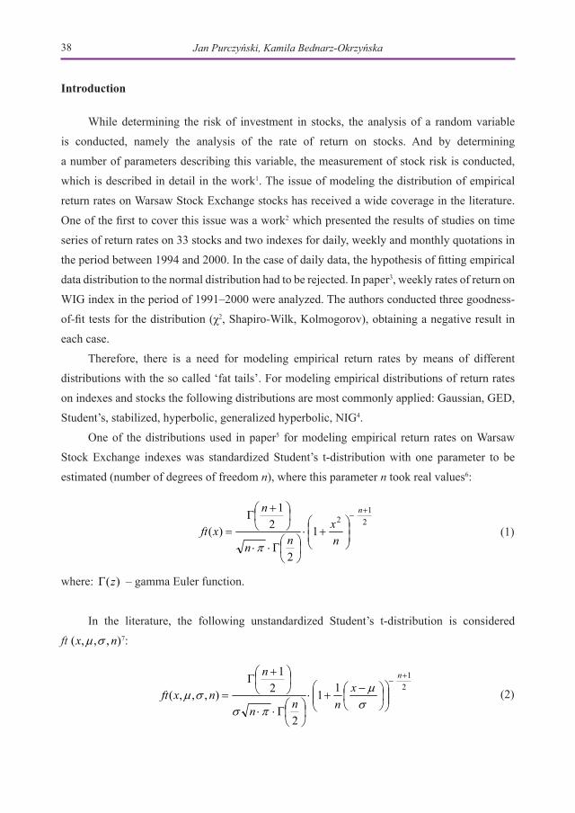
One of the distributions used in paper5 for modeling empirical return rates on Warsaw

Stock Exchange indexes was standardized Student’s t-distribution with one parameter to be

estimated (number of degrees of freedom n), where this parameter n took real values6:

2

12

1

2

21

)(

n

nx

nn

n

xft

(1)

where: )(zΓ – gamma Euler function.

In the literature, the following unstandardized Student’s t-distribution is considered

ft ),,,( nxft σµ 7:

2

111

2

21

),,,(

nx

nnn

n

nxft

(2)

Application of Generalized Student’s t-Distribution... 39

where:

μ – location parameter,

σ – scale parameter,

n – number of degrees of freedom.

1. Estimation of parameters of generalized Student’s t-distribution

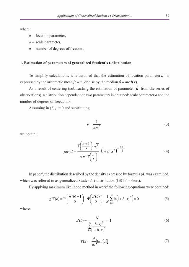
To simplify calculations, it is assumed that the estimation of location parameter µ̂ is

expressed by the arithmetic mean x=µ̂ , or else by the median )(ˆ xmed=µ .

As a result of centering (subtracting the estimation of parameter µ̂ from the series of

observations), a distribution dependent on two parameters is obtained: scale parameter σ and the

number of degrees of freedom n.Assuming in (2) μ = 0 and substituting

21σn

b = (3)

we obtain:

21

21

2

21

)(

n

xbn

bn

xfut

(4)

In paper8, the distribution described by the density expressed by formula (4) was examined,

which was referred to as generalized Student’s t-distribution (GST for short).

By applying maximum likelihood method in work9 the following equations were obtained:

N

kkxb

NbnbnbgW

1

2 01ln12

)(2

1)()( (5)

where:

1

1

)(

12

2 −

⋅+⋅

=′

∑=

N

k k

k

xbxb

Nbn (6)

zdzdz ln)( (7)


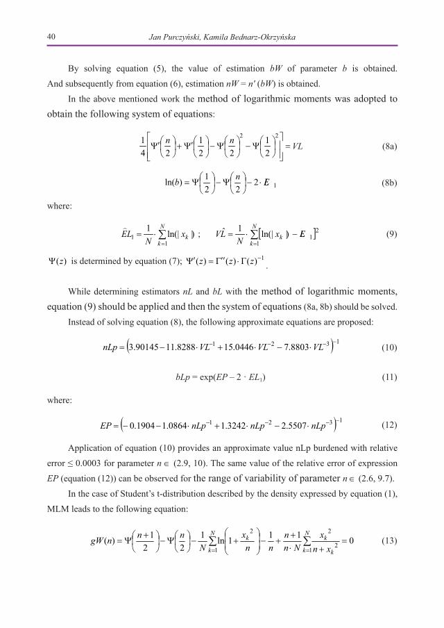
By solving equation (5), the value of estimation bW of parameter b is obtained.

And subsequently from equation (6), estimation nW = n' (bW) is obtained.

In the above mentioned work the method of logarithmic moments was adopted to obtain the following system of equations:

VLnn=

Ψ−

Ψ−

Ψ′+

Ψ′

22

21

221

241 VL (8a)

1222

1)ln( ELnb ⋅−

Ψ−

Ψ= (8b)

where:

∑=

⋅=N

kkx

NLE

11 |)ln(|1

; [ ]∑=

−⋅=N

kk ELx

NLV

1

21|)ln(|1ˆ (9)

)(zΨ is determined by equation (7); 1)()()( −Γ⋅Γ ′′=Ψ′ zzz .

While determining estimators nL and bL with the method of logarithmic moments, equation (9) should be applied and then the system of equations (8a, 8b) should be solved.

Instead of solving equation (8), the following approximate equations are proposed:

1321 8803.70446.158288.1190145.3 VLVLVLnLp (10)

bLp = exp(EP – 2 · EL1) (11)

where:

1321 5507.23242.10864.11904.0 nLpnLpnLpEP (12)

Application of equation (10) provides an approximate value nLp burdened with relative

error ≤ 0.0003 for parameter n ∈ (2.9, 10). The same value of the relative error of expression

EP (equation (12)) can be observed for the range of variability of parameter n ∈ (2.6, 9.7).

In the case of Student’s t-distribution described by the density expressed by equation (1),

MLM leads to the following equation:

N

k

N

k k

kk

xnx

Nnn

nnx

NnnngW

1 12

220111ln1

221)( (13)


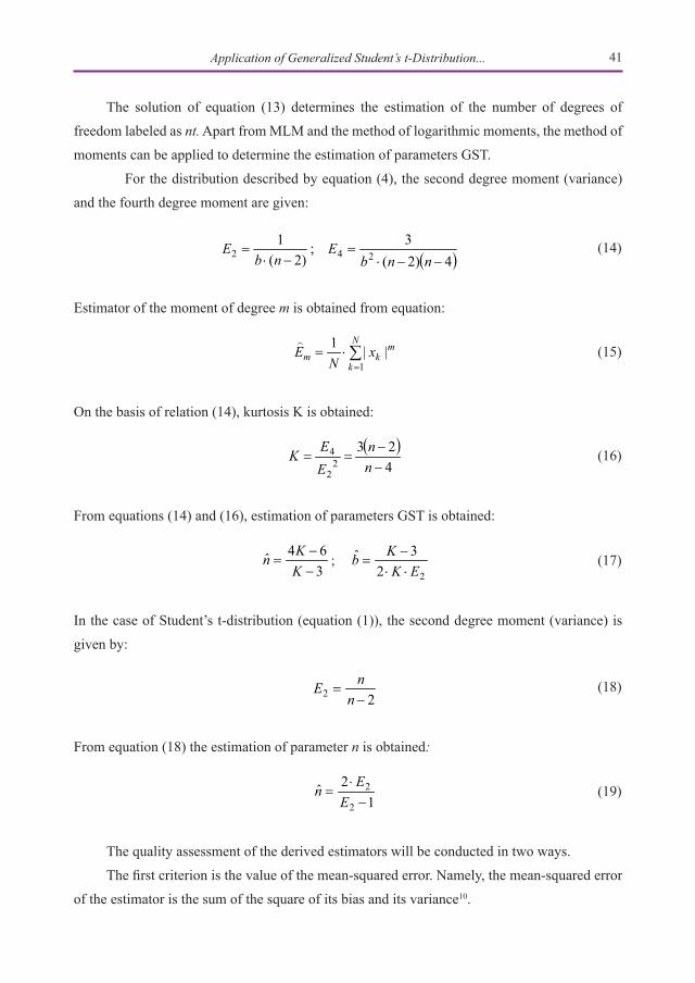
The solution of equation (13) determines the estimation of the number of degrees of

freedom labeled as nt. Apart from MLM and the method of logarithmic moments, the method of

moments can be applied to determine the estimation of parameters GST.

For the distribution described by equation (4), the second degree moment (variance)

and the fourth degree moment are given:

)2(

12

nbE ;

4)2(3

24

nnb

E (14)

Estimator of the moment of degree m is obtained from equation:

∑=

⋅=N

k

mkm x

NE

1||1

(15)

On the basis of relation (14), kurtosis K is obtained:

( )423

22

4

−−

==nn

EEK (16)

From equations (14) and (16), estimation of parameters GST is obtained:

364ˆ

−−

=KKn ;

223ˆEK

Kb⋅⋅

−= (17)

In the case of Student’s t-distribution (equation (1)), the second degree moment (variance) is

given by:

22 −

=n

nE (18)

From equation (18) the estimation of parameter n is obtained:

1

2ˆ2

2

−⋅

=E

En (19)

The quality assessment of the derived estimators will be conducted in two ways.

The first criterion is the value of the mean-squared error. Namely, the mean-squared error

of the estimator is the sum of the square of its bias and its variance10.


The second criterion, resulting from the fact that the paper is concerned with modeling

empirical distributions of return rates on indexes and stocks, is the value of chi-squared test

statistic. The latter criterion is superior, since the aim of the proposed method is the approximation

of empirical distributions of return rates on stock indexes.

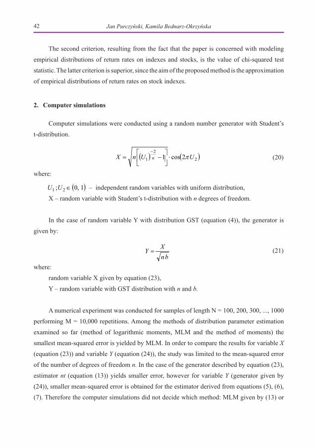
2. Computer simulations

Computer simulations were conducted using a random number generator with Student’s

t-distribution.

( ) ( )2

2

1 2cos1 UUnX n π⋅

−=

− (20)

where:

( )1,0; 21 ∈UU – independent random variables with uniform distribution,

X – random variable with Student’s t-distribution with n degrees of freedom.

In the case of random variable Y with distribution GST (equation (4)), the generator is

given by:

bn

XY = (21)

where:

random variable X given by equation (23),

Y – random variable with GST distribution with n and b.

A numerical experiment was conducted for samples of length N = 100, 200, 300, ..., 1000

performing M = 10,000 repetitions. Among the methods of distribution parameter estimation

examined so far (method of logarithmic moments, MLM and the method of moments) the

smallest mean-squared error is yielded by MLM. In order to compare the results for variable X

(equation (23)) and variable Y (equation (24)), the study was limited to the mean-squared error

of the number of degrees of freedom n. In the case of the generator described by equation (23),

estimator nt (equation (13)) yields smaller error, however for variable Y (generator given by

(24)), smaller mean-squared error is obtained for the estimator derived from equations (5), (6),

(7). Therefore the computer simulations did not decide which method: MLM given by (13) or


MLM given by (5), (6), and (7) is more useful in the estimation of the number of degrees of

freedom n.

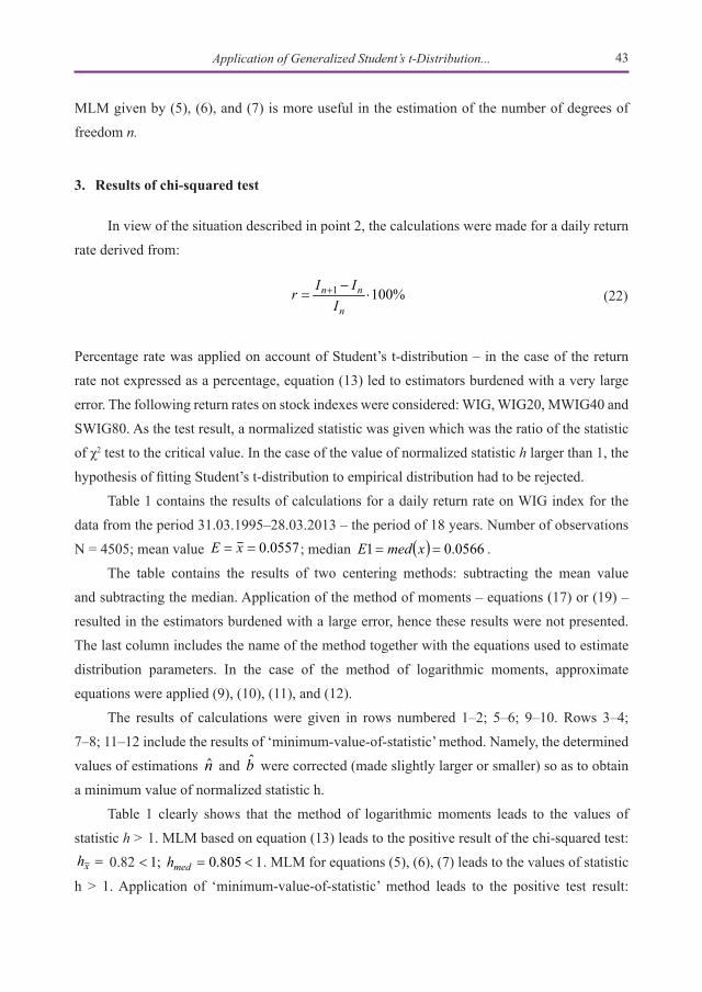
3. Results of chi-squared test

In view of the situation described in point 2, the calculations were made for a daily return

rate derived from:

%1001 ⋅−

= +

n

nn

IIIr (22)

Percentage rate was applied on account of Student’s t-distribution – in the case of the return

rate not expressed as a percentage, equation (13) led to estimators burdened with a very large

error. The following return rates on stock indexes were considered: WIG, WIG20, MWIG40 and

SWIG80. As the test result, a normalized statistic was given which was the ratio of the statistic

of χ2 test to the critical value. In the case of the value of normalized statistic h larger than 1, the

hypothesis of fitting Student’s t-distribution to empirical distribution had to be rejected.

Table 1 contains the results of calculations for a daily return rate on WIG index for the

data from the period 31.03.1995–28.03.2013 – the period of 18 years. Number of observations

N = 4505; mean value 0557.0== xE ; median ( ) 0566.01 == xmedE .

The table contains the results of two centering methods: subtracting the mean value

and subtracting the median. Application of the method of moments – equations (17) or (19) –

resulted in the estimators burdened with a large error, hence these results were not presented.

The last column includes the name of the method together with the equations used to estimate

distribution parameters. In the case of the method of logarithmic moments, approximate

equations were applied (9), (10), (11), and (12).

The results of calculations were given in rows numbered 1–2; 5–6; 9–10. Rows 3–4;

7–8; 11–12 include the results of ‘minimum-value-of-statistic’ method. Namely, the determined

values of estimations n̂ and b̂ were corrected (made slightly larger or smaller) so as to obtain

a minimum value of normalized statistic h.

Table 1 clearly shows that the method of logarithmic moments leads to the values of

statistic h > 1. MLM based on equation (13) leads to the positive result of the chi-squared test: 1805.0;182.0 <=<= medx hh 0.82 1805.0;182.0 <=<= medx hh . MLM for equations (5), (6), (7) leads to the values of statistic

h > 1. Application of ‘minimum-value-of-statistic’ method leads to the positive test result:


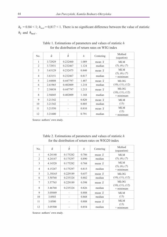
xh = 0.84 < 1; hmed = 0,817 < 1. There is no significant difference between the value of statistic

xh and medh .

Table 1. Estimations of parameters and values of statistic h for the distribution of return rates on WIG index

No. n̂ b̂ h Centering Method (equation)

1 3.72929 0.232460 1.089 mean x MLM(5), (6), (7)2 3.72931 0.232467 1.124 median

3 3.63129 0.232475 0.840 mean x MLM(5), (6), (7)+ minimum4 3.63151 0.232467 0.817 median

5 2.44808 0.447797 1.487 mean x MLOG(10), (11), (12)6 2.61965 0.402009 1.218 median

7 2.38838 0.447797 1.215 mean x MLOG(10), (11), (12)

+ minimum8 2.56045 0.402009 1.168 median

9 3.21342 – 0.820 mean x MLM(13)10 3.21342 – 0.805 median

11 3.21550 – 0.810 mean x MLM(13)

+ minimum12 3.21600 – 0.791 median

Source: authors’ own study.

Table 2. Estimations of parameters and values of statistic h for the distribution of return rates on WIG20 index

No. n̂ b̂ h Centering Method (equaution)

1 4.24148 0.175282 0.786 mean x MLM(5), (6), (7)2 4.24147 0.175297 0.890 median


5 3,.58165 0.229189 0.657 mean x MLOG(10), (11), (12)6 3.50768 0.235324 0.882 median

7 3.57765 0.229189 0.598 mean x MLOG(10), (11), (12)

+ minimum8 3.46768 0.235324 0.826 median

9 3.05049 – 0.888 mean x MLM(13)10 3.0503 – 0.868 median

11 3.0500 – 0.888 mean x MLM(13)

+ minimum12 3.05500 – 0.854 median



Table 2 contains the results of calculations for a daily return rate on WIG20 index for the


N = 2761; mean value 0333.0== xE ; median ( ) 0477.01 == xmedE .

All the methods lead to the positive result of the chi-squared test. In the case of the

generalized Student’s t-distribution (rows 1–8), mean-centering yields smaller values of statistic

h than by subtracting the median. The smallest value of the statistic is obtained for the method

of logarithmic moments 657.0=xh , also after correction 598.0min =xh .

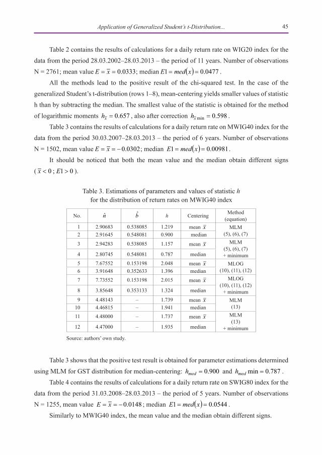
Table 3 contains the results of calculations for a daily return rate on MWIG40 index for the


N = 1502, mean value 0302.0−== xE ; median ( ) 00981.01 == xmedE .

It should be noticed that both the mean value and the median obtain different signs

( 01;0 >< Ex ).

Table 3. Estimations of parameters and values of statistic h for the distribution of return rates on MWIG40 index

No. n̂ b̂ h Centering Method (equation)

1 2.90683 0.538085 1.219 mean x MLM(5), (6), (7)2 2.91645 0.548081 0.900 median



7 7.73552 0.153198 2.015 mean x MLOG(10), (11), (12)

+ minimum8 3.85648 0.353133 1.324 median

9 4.48143 – 1.739 mean x MLM(13)10 4.46815 – 1.941 median

11 4.48000 – 1.737 mean x MLM(13)

+ minimum12 4.47000 – 1.935 median


Table 3 shows that the positive test result is obtained for parameter estimations determined

using MLM for GST distribution for median-centering: 900.0=medh and 787.0min =medh .

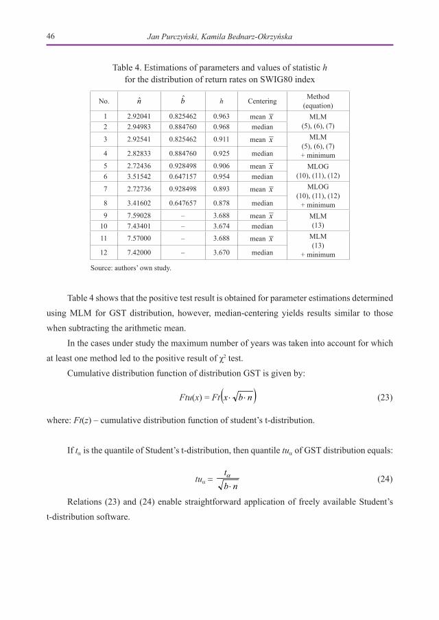
Table 4 contains the results of calculations for a daily return rate on SWIG80 index for the


N = 1255, mean value 0148.0−== xE ; median ( ) 0544.01 == xmedE .

Similarly to MWIG40 index, the mean value and the median obtain different signs.


Table 4. Estimations of parameters and values of statistic h for the distribution of return rates on SWIG80 index

No. n̂ b̂ h Centering Method(equation)

1 2.92041 0.825462 0.963 mean x MLM(5), (6), (7)2 2.94983 0.884760 0.968 median



7 2.72736 0.928498 0.893 mean x MLOG(10), (11), (12)

+ minimum8 3.41602 0.647657 0.878 median

9 7.59028 – 3.688 mean x MLM(13)10 7.43401 – 3.674 median

11 7.57000 – 3.688 mean x MLM(13)

+ minimum12 7.42000 – 3.670 median


Table 4 shows that the positive test result is obtained for parameter estimations determined

using MLM for GST distribution, however, median-centering yields results similar to those

when subtracting the arithmetic mean.

In the cases under study the maximum number of years was taken into account for which

at least one method led to the positive result of χ2 test.

Cumulative distribution function of distribution GST is given by:

Ftu(x) = Ft ( )nbxFtxFtu ⋅⋅=)( (23)

where: Ft(z) – cumulative distribution function of student’s t-distribution.

If ta is the quantile of Student’s t-distribution, then quantile tua of GST distribution equals:

tua = nb

ttu⋅

= aa (24)

Relations (23) and (24) enable straightforward application of freely available Student’s

t-distribution software.


Conclusions

The research aim was to compare the applicability of Student’s t-distribution (equation

(1)) and generalized Student’s t-distribution (equation (4)) in modeling empirical return rates

on selected exchange indexes. Furthermore, an attempt was made to ascertain which estimator

of location parameter: arithmetic mean x=µ̂ , or median )(ˆ xmed=µ proves more useful in

the process of centering (subtraction of parameter µ̂ estimation from a series of observations).

To summarize the results of modeling the distribution of return rates described in point 3,

it should be noticed that GST distribution provided a positive result of the chi-squared test in

all the considered cases. By contrast, Student’s t-distribution proved useful in only two cases

(Tables 1 and 2). It means that GST distribution ensures better fitting to empirical data than the

classical Student’s t-distribution.

While comparing two methods of centering, no clear advantage of either method can be

observed: in one case (Table 3) the subtraction of median yields better results, in another case

(Table 2) the subtraction of arithmetic mean yields smaller values of normalized statistic, and in

two other cases (Tables 1 and 4) the results are similar. Therefore, the practical conclusion is that

centering should be done using both methods, and as a final result the variant yielding a smaller

value of normalized statistic should be chosen.

Notes

1 Tarczyński, Mojsiewicz (2001), pp. 61–84.2 Jajuga (2000).3 Tarczyński, Mojsiewicz (2001), pp. 55–58.4 Weron, Weron (1998), pp. 285–291; Mantegna, Stanley (2001); Purczyński, Guzowska (2002), pp. 105–118;

Tomasik E. (2011). 5 Ibidem6 Shaw (2006), pp. 37–73.7 Sutradhar (1986), pp. 329–337; Jackman (2009).8 Purczyński (2003), pp. 147.9 Ibidem, pp. 149–150.

10 Krzyśko (1997)


References

Jackman, S. (2009). Bayesian analysis for the social sciences. New York: Wiley.

Jajuga, K. (2000). Econometric and statistical methods in the capital market analysis. Wrocław: Wydawnictwo Akademii Ekonomicznej.

Krzyśko, M. (1997). Mathematical statistics. Cz. II, Poznań: UAM.

Mantegna, R.N. & Stanley, H.E. (2001). Econophysics. Warszawa: Wydawnictwo Naukowe PWN.

Purczyński, J. & Guzowska, M. (2002): Application of a -stabilized and GED Distributions in Modeling the Distribution of Return Rates on S&P500 Index, conference materials ,,Capi-tal Market – Effective Investing” Vol. 1. Szczecin: Wydawnctwo Naukowe Uniwersytetu Szczecińskiego.

Purczyński, J. (2003). Application of computer simulations to estimation of selected economet-ric and statistical models. Uniwersytet Szczeciński, Rozprawy i Studia T. (DXXV), 451, Szczecin: Wydawnctwo Naukowe Uniwersytetu Szczecińskiego.

Shaw, W.T. (2006), Sampling Student`s T distribution – use of the inverse cumulative distribu-tion function, Journal of Computational Finance, Vol. 9, No. 4.

Sutradhar, B.C. (1986). On the characteristic function of multivariate Student t-distribution. Canadian Journal of Statistics 14.

Tarczyński, W. & Mojsiewicz, M. (2001). Risk management. Warszawa: PWE.

Tomasik, E. (2011). Analysis of rates of return distributions of financial instruments on Polish capital market. Doctoral dissertation, Uniwersytet Ekonomiczny w Poznaniu, Poznań.

Weron, A. & Weron, R. (1998). Financial engineering. Warszawa: WNT.

jan purczyński, kamila...

Documents