johansen, s. (1988) - statistical analysis of cointegration vectors

Journal of Economic Dynamics and Control 12 (1988) 231-254. North-Holland

STATISTICAL ANALYSIS OF COINTEGRATION VECTORS

Soren JOHANSEN*

University of Copenhagen, DK-2100 Copenhagen, Denmark

Received September 1987, final version received January 1988

We consider a nonstationary vector autoregressive process which is integrated of order 1, and generated by i.i.d. Gaussian errors. We then derive the maximum likelihood estimator of the space of cointegration vectors and the likelihood ratio test of the hypothesis that it has a given number of dimensions. Further we test linear hypotheses about the cointegration vectors.

The asymptotic distribution of these test statistics are found and the first is described by a natural multivariate version of the usual test for unit root in an autoregressive process, and the other is a x2 test.

1. Introduction

The idea of using cointegration vectors in the study of nonstationary time series comes from the work of Granger (1981), Granger and Weiss (1983), Granger and Engle (1985), and Engle and Granger (1987). The connection with error correcting models has been investigated by a number of authors; see Davidson (1986), Stock (1987), and Johansen (1988) among others.

Granger and Engle (1987) suggest estimating the cointegration relations using regression, and these estimators have been investigated by Stock (1987), Phillips (1985), Phillips and Durlauf (1986), Phillips and Park (1986a, b, 1987), Phillips and Ouliaris (1986,1987), Stock and Watson (1987), and Sims, Stock and Watson (1986). The purpose of this paper is to derive maximum likelihood estimators of the cointegration vectors for an autoregressive process with independent Gaussian errors, and to derive a likelihood ratio test for the hypothesis that there is a given number of these. A similar approach has been taken by Ahn and Reinsel (1987).

This program will not only give good estimates and test statistics in the Gaussian case, but will also yield estimators and tests, the properties of which can be investigated under various other assumptions about the underlying data generating process. The reason for expecting the estimators to behave better

*The simulations were carefully performed by Marc Andersen with the support of the Danish Social Science Research Council. The author is very grateful to the referee whose critique of the first version greatly helped improve the presentation.

0165-1889/88/$3,5001988, Elsevier Science Publishers B.V. (North-Holland)

J.E.D.C.--B

232 S. Johansen, Statistical analysis of cointegration vectors

than the regression estimates is that they take into account the error structure of the underlying process, which the regression estimates do not.

The processes we shall consider are defined from a sequence {E,} of i.i.d. p-dimensional Gaussian random variables with mean zero and variance matrix

A. We shall define the process X, by

x,=n,x,_,+ ... +t~X,_,+E,, t=1,2 >.‘., (1)

for given values of X_ k + i, . . , X0. We shall work in the conditional distribution given the starting values, since we shall allow the process X, to be nonstationary. We define the matrix polynomial

A(z)=I-qz- ... -n,z”,

and we shall be concerned with the situation where the determinant IA(z)/ has roots at z = 1. The general structure of such processes and the relation to error correction models was studied in the above references.

We shall in this paper mainly consider a very simple case where X, is integrated of order 1, such that AX, is stationary, and where the impact matrix

A(z)l,=,=II=I-II,- ... -nk

has rank r <p. If we express this as

Ill = (Yp, (2)

for suitable p X r matrices (Y and fi, then we shall assume that, although AX, is stationary and X, is nonstationary as a vector process, the linear combinations given by P’X, are stationary. In the terminology of Granger this means that the vector process X, is cointegrated with cointegration vectors p_ The space spanned by /3 is the space spanned by the rows of the matrix II, which we shall call the cointegration space.

In this paper we shall derive the likelihood ratio test for the hypothesis given by (2) and derive the maximum likelihood estimator of the cointegration space. Then we shall find the likelihood ratio test of the hypothesis that the cointegration space is restricted to lie in a certain subspace, representing the linear restrictions that one may want to impose on the cointegration vectors.

The results we obtain can briefly be described as follows: the estimation of /I is performed by first regressing AX, and X,_, on the lagged differences. From the residuals of these 2p regressions we calculate a 2p X 2p matrix of product moments. We can now show that the estimate of p is the empirical canonical variates of X,-, with respect to AX, corrected for the lagged differences.

S. Johansen, Statistical analysis of cointegration vectors 233

The likelihood ratio test is now a function of certain eigenvalues of the product moment matrix corresponding to the smallest squared canonical correlations. The test of the linear restrictions involve yet another set of eigenvalues of a reduced product moment matrix. The asymptotic distribution of the first test statistic involves an integral of a multivariate Brownian motion with respect to itself, and turns out to depend on just one parameter, namely the dimension of the process, and can hence be tabulated by simulation or approximated by a X2 distribution. The second test statistic is asymptotically distributed as x2 with the proper degrees of freedom. It is also shown that the maximum likelihood estimator of p suitably normalised is asymptotically distributed as a mixture of Gaussian variables.

2. Maximum likelihood estimation of cointegration vectors and likelihood ratio tests of hypotheses about cointegration vectors

We want to estimate the space spanned by /3 from observations X,, t= -k+l,..., T. For any r up we formulate the model as the hypothesis

H,: rank(n) 5 r or II= a/?‘, (3)

where (Y and /3 are p x r matrices. Note that there are no other constraints on II,, . . . , Ilk than (3). Hence a

wide class containing stationary as well as nonstationary processes is considered.

The parameters (Y and p can not be estimated since they form an over- parametrisation of the model, but one can estimate the space spanned by fi.

We can now formulate the main result about the estimation of sp(p) and the test of the hypothesis (3).

Theorem I. The maximum likelihood estimator of the space spanned by p is the space spanned by the r canonical variates corresponding to the r largest squared

canonical correlations between the residuals of X,_, and AX, corrected for the

efSect of the lagged dtferences of the X process. The likelihood ratio test statistic for the hypothesis that there are at most r

cointegration vectors is

-2ln(Q) = -T i ln(l -A;), (4) i=r+l

where i ,.+ 1, . . . , ip are the p - r smallest squared canonical correlations.

Proof. Before studying the likelihood function it is convenient to reparame- trise the model (1) such that the parameter of interest II enters explicitly. We


write

AX,=T,AX,_,+ .a. +rk-lAX+k+l+I’kXt_k+~,, (5)

where

r, = -I+&+ *** +ni, i=l ,a*., k.

Then IT = -r,, and whereas (3) gives a nonlinear constraint on the coefficients n,, . . . , IIk, the parameters (I’,, . . . , rk_l, a, B, A) have no constraints imposed. In this way the impact matrix II is found as the coefficient of the lagged levels in a nonlinear least squares regression of AX, on lagged differences and lagged levels. The maximisation over the parameters r,, . . . , I’,_ 1 is easy since it just leads to an ordinary least squares regression of AX, + (Y/?‘X,_~ on the lagged differences. Let us do this by first regressing AX, on the lagged differences giving the residuals R,, and then regressing X,_, on the lagged differences giving the residuals R,,. After having performed these regressions the concentrated likelihood function becomes proportional to

WrJ4.N

0, + @R,,)‘A-‘(Ro, + d’R,,)

For fixed p we can maximise over OL and A by a usual regression of R,, on -j3’Rk, which gives the well-known result

and

W) = -So,PWS,,P)-‘~ (6)

A(P) = Soo- S0,PW&,P)%%0~ (7)

where we have defined product moment matrices of the residuals as

Sij = T-’ ; R,,R(,, i, j = 0, k. t-l

(8)

The likelihood profile now becomes proportional to

and it remains to solve the minimisation problem

mWS, - So,B(P’S,,P)-‘P’S,oI,

where the minimisation is over all p x r matrices /3. The well-known matrix


relation [see Rao (1973)]

= IP'skkplISoo-SokP(p'SkkP)-lp'SkOI

shows that we shall minimise

with respect to the matrix /I. We now let D denote the diagonal matrix of ordered eigenvalues fir > . - *

> ip of SkOS&,?!$,, with respect to Skk, i.e., the solutions to the equation

Ixs,, - S,,S&‘S,,,] = O, (9)

and E the matrix of the corresponding eigenvectors, then

S,,ED = S,,&&,,E,

where E is normalised such that

E’S,, E = I.

Now choose p = Et where E is p X r, then we shall minimise

IE’E - E’DEI/IE’EI.

This can be accomplished by choosing E to be the first r unit vectors or by choosing B to be the first r eigenvectors of S,#!&‘SOk with reSpeCt to Skk, i.e., the first r columns of E. These are called the canonical variates and the eigenvalues are the squared canonical correlations of R, with respect to R,. For the details of these calculations the reader is referred to Anderson (1984, ch. 12). This type of analysis is also called reduced rank regression [see Ahn and Reinsel (1987) and Velu, Reinsel and Wichem (1986)]. Note that all possible choices of the optimal p can be found from B by j3 = /$I for p an r X r matrix of full rank. The eigenvectors are normalised by the condition B’SkkB = Z such that the estimates of the other parameters are given by

& = - S,,,& ,&S,&& -’ = -S,,,&

which clearly depends on the choice of the optimising p, whereas

(10)

‘= -s,,fi(,@k&-lfj,= -SOk,j/ftr (11)


(12)

L,Z’= IS,l fJ (1 -A,>, 03) r=l

do not depend on the choice of optimising p. With these results it is easy to find the estimates of II and A without the

constraint (3). These follow from (6) and (7) for r =p and /I = I and give in particular the maximised likelihood function without the constraint (3):

L-2’T= ,S,, JJ (1 -A,>. max 04)

If we now want a test that there are at most r cointegrating vectors, then the likelihood ratio test statistic is the rftio of (13) and (14) which can be expressed as (4) where ir+l > . . . > A,, are the p - r smallest eigenvalues. This completes the proof of Theorem 1.

Notice how this analysis allows one to calculate all p eigenvalues and eigenvectors at once, and then make inference about the number of important cointegration relations, by testing how many of the h’s are zero.

Next we shall investigate the test of a linear hypothesis about j3. In the case we have Y = 1, i.e., only one cointegration vector, it seems natural to test that certain variables do not enter into the cointegration vector, or that certain linear constraints are satisfied, for instance that the variables Xi, and X,, only enter through their difference Xi, - X,,. If r 2 2, then a hypothesis of interest could be that the variables Xi, and X,, enter through their difference only in all the cointegration vectors, since if two different linear combinations would occur then any coefficients to Xi, and X,, would be possible. Thus it seems that some natural hypotheses on p can be formulated as

Hi: P=%, (15)

where H( p x s) is a known matrix of full rank s and q(s x r) is a matrix of unknown parameters. We assume that r I s up. If s =p, then no restrictions are placed upon the choice of cointegration vectors, and if s = r, then the cointegration space is fully specified.

Theorem 2. The maximum likelihood estimator of the cointegration space, under the assumption that it is restricted to sp( H), is given as the space spanned


by the canonical variates corresponding to the r largest squared canonical correlations between the residuals of H’X,_, and AX, corrected for the lagged diflerences of X,.

The likelihood ratio test now becomes

-2ln(Q)=Tiln((l-X:)/(1-i;)), i=l

(16)

where Xl;, . . . , A: are the r largest squared canonical correlations.

Proof. It is apparent from the derivation of p^ that if p = Hq is fixed, then regression of R,, on -‘p’H’R,, is still a simple linear regression and the analysis is as before with R,, replaced by H’R,,. Thus the matrix ‘p can be estimated as the eigenvectors corresponding to the r largest eigenvalues of

H’S,,S&,‘S,,, H with respect to H’S,,H, i.e., the solution to

IXH’S,,H - H’S,,&&HI = 0.

Let the s eigenvalues be denoted by hy, i = 1,. . . , s. Then the likelihood ratio test of Hi in H, can be found from two expressions like (13) and is given by (16), which completes the proof of Theorem 2.

In the next section we shall find the asymptotic distribution of the test statistics (4) and (16) and show that the cointegration space, the impact matrix II and the variance matrix A are estimated consistently.

3. Asymptotic properties of the estimators and the test statistics

In order to derive properties of the estimators we need to impose more precise conditions on the parameters of the model, such that they correspond to the situation we have in mind, namely of a process that is integrated of order 1, but still has r cointegration vectors fi.

First of all we want all roots of \A( z)l = 0 to satisfy lz I > 1 or possibly z = 1. This implies that the nonstationarity of the process can be removed by differencing. Next we shall assume that X, is integrated of order 1, i.e., that AX, is stationary and that the hypothesis (3) is satisfied by some (Y and p of full rank r. Correspondingly we can express AX, in terms of the e’s by its moving average representation,

AX,= f- C-p-/~ J=o

for some exponentially decreasing coefficients C,. Under suitable conditions on these coefficients it is known that this equation determines an error correction


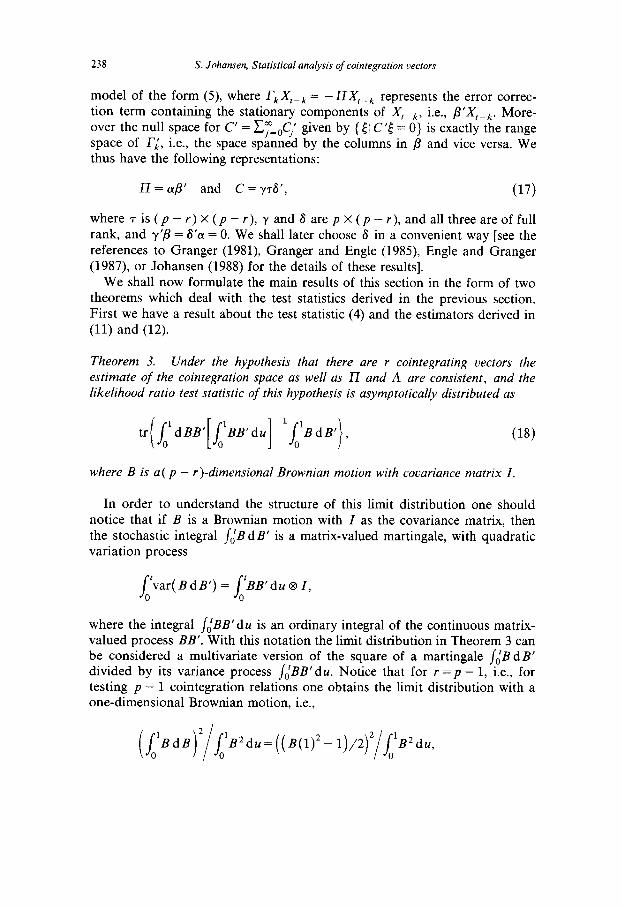
model of the form (5), where r,X,_, = -IIX,_, represents the error correction term containing the stationary components of X,_k, i.e., B’Xt_k. More- over the null space for C’ = c,“=&.’ given by {[I C’[ = 0} is exactly the range space of r,l, i.e., the space spanned by the columns in B and vice versa. We thus have the following representations:

II=@’ and C=yr8’, (17)

where 7 is ( p - r) X (p - r), y and 6 are p X ( p - r), and all three are of full rank, and y’B = B’(Y = 0. We shall later choose 6 in a convenient way [see the references to Granger (1981) Granger and Engle (1985), Engle and Granger (1987) or Johansen (1988) for the details of these results].

We shall now formulate the main results of this section in the form of two theorems which deal with the test statistics derived in the previous section. First we have a result about the test statistic (4) and the estimators derived in (11) and (12).

Theorem 3. Under the hypothesis that there are r cointegrating vectors the estimate of the cointegration space as well as IT and A are consistent, and the likelihood ratio test statistic of this hypothesis is asymptotically distributed as

tr( /o’dBB’[ L’BB’du] -‘l’B dB’), (18)

where B is a( p - r)-dimensional Brownian motion with covariance matrix I.

In order to understand the structure of this limit distribution one should notice that if B is a Brownian motion with I as the covariance matrix, then the stochastic integral /ofB d B’ is a matrix-valued martingale, with quadratic variation process

/‘var(BdB’)=/‘BB’duQI, 0 0

where the integral _/,,‘BB’du is an ordinary integral of the continuous matrix- valued process BB’. With this notation the limit distribution in Theorem 3 can be considered a multivariate version of the square of a martingale /ofB d B’ divided by its variance process /,,‘BB’du. Notice that for r =p - 1, i.e., for testing p - 1 cointegration relations one obtains the limit distribution with a one-dimensional Brownian motion, i.e.,

(~1BdB)~~1B2du=((B(1)2-1),Z)Y11B2dU, 0

S. Johansen, Statistical analysis of coiniegration vectors 239

Table 1

The quantiles in the distribution of the test statistic,

where B is an m-dimensional Brownian motion with covariance matrix I.

m 2.5% 5% 10% 50% 90% 95% 97.5%

1 0.0 0.0 0.0 0.6 2.9 4.2 5.3 2 1.6 1.9 2.5 5.4 10.3 12.0 13.9 3 7.0 7.8 8.8 14.0 21.2 23.8 26.1 4 16.0 17.4 19.2 26.3 35.6 38.6 41.2 5 28.3 30.4 32.8 42.1 53.6 57.2 60.3

which is the square of the usual ‘unit root’ distribution [see Dickey and Fuller (1979)]. A similar reduction is found by Phillips and Ouliaris (1987) in their work on tests for cointegration based on residuals. The distribution of the test statistic (18) is found by simulation and given in table 1.

A surprisingly accurate description of the results in table 1 is obtained by approximating the distributions by cx2(f) for suitable values of c and f. By equating the mean of the distributions based on 10,000 observations to those of cx2 with f = 2m2 degrees of freedom, we obtain values of c, and it turns out that we can use the empirical relation

c = 0.85 - 0.58/f.

Notice that the hypothesis of r cointegrating relations reduces the number of parameters in the II matrix from p2 to rp + r( p - r), thus one could expect ( p - r)2 degrees of freedom if the usual asymptotics would hold. In the case of nonstationary processes it is known that this does not hold but a very good approximation is given by the above choice of 2( p - r)2 degrees of freedom.

Next we shall consider the test of the restriction (15) where linear constraints are imposed on j3.

Theorem 4. The likelihood ratio test of the hypothesis

Hi: P=&

of restricting the r-dimensional cointegration space to an s-dimensional subspace of RP is asymptotically distributed as x2 with r( p - s) degrees of freedom.

We shall now give the proof of these theorems, through a series of inter- mediate results. We shall first give some expressions for variances and their

240 S. Johansen, Statistical analysis ojcointegrution uectors

limits, then show how the algorithm for deriving the maximum likelihood estimator can be followed by a probabilistic analysis ending up with the asymptotic properties of the estimator and the test statistics.

We can represent X, as X, = c:=, A Xi, where X0 is a constant which we shall take to be zero to simplify the notatton. We shall describe the stationary process AX, by its covariance function

q(i) = var(AX,, AX,+,),

and we define the matrices

p,, =$(i -j) = E(AX,_,AX,‘,), i, j=O ,...,k-1,

i=O ,..., k- 1,

and

P kk= -

/=-CC

Finally define

Note the following relations:

J=o J=o

r-k

var(x,-k)= C (t-k- ljl)G(j),

J=-t+k

*--I

COV( x,-k, Ax,-i) = c ‘b(j), j=k-1

S. Johansen, Sratistical analysis of cointegration vectors 241

which show that

var(X,/T1/2) -+ f 4(j) =+, I=--m

and

cov( xTpk, AX,_,) --) f q(j) = P/cry j=k-r

whereas the relation

T-k T-k

var(p’xT-k) = tTek) c b’+(j)/?- c i_db’+(j)P

/= -T+k j= -T+k

shows that

since P’C = 0 implies that P’J, = 0, such that the first term vanishes in the limit. Note that the nonstationary part of X, makes the variance matrix tend to infinity, except for the directions given by the vectors in fi, since P’X, is

stationary. The calculations involved in the maximum likelihood estimation all center

around the product moment matrices

M,, = ~-1 i Ax,_,Ax;-,, i, j=O ,...,k-1, r=l

Mki = T-’ i X,_,AX,‘i, i=O,...,k-1, t=l

Mkk = T-’ ; X,-,x;-, t=1

We shall first give the asymptotic behaviour of these matrices, then find the asymptotic properties of S,, and finally apply these results to the estimators and the test statistic. The methods are inspired by Phillips (1985) even though I shall stick to the Gaussian case, which make the arguments somewhat simpler.

The following lemma can be derived by the results in Phillips and Durlauf (1986). We let W be a Brownian motion in p dimensions with covariance matrix A.


Lemma 1. As T + 00, we have

T-1’2XuTtl : CW( t), 09)

a.s.

Mij + Pij, i, j=O ,..., k- 1, (20)

Mki 4 C/lWdw’C’ + pki, i=O,..., k- 1, (21) 0

T-lMkk: Cjo’W(u)W’(u)du C’. (23)

Note that for any E E RP, E’M,& is of the order in probability of T unless 6 is in the space spanned by /3, in which case it is convergent. Note also that the stochastic integrals enter as limits of the nonstationary part of the process X,, and that they disappear when multiplied by /?, since P’C = 0.

We shall apply the results to find the asymptotic properties of Sij, i, j = 0, k, see (8). These can be expressed in terms of the Mij’s as follows:

Sij = Mij - M,,M,-:M,,, i, j = 0, k,

where

M**= {Mij, i, j=l,..., k-l},

Mk*= {Mki, i=l,..., k-l},

MO*= {Moi, i=l,..., k-l}.

A similar notation is introduced for the pij’s. It is convenient to have the notation

Bij= Pij- Pi*PGb*j% i, j=O,k.

We now get:

Lemma 2. The following relations hold

z,=r,z,,+n,

&/J~ = r/J/&G,

(24)

(25)


and hence, since r, = -a/?‘.

Z00=~(jl’2kk~)~‘+A and 1y= -B,,/?(~‘B,,~)-l. (26)

Proof. From the defining eq. (5) for the process X, we find the equations

i& = r,iV,, + - * * +I’k_1Mk._l,i + &Mki + T-’ t e,AX:-iy (27) r-1

i=O,l ,..., k- 1, and

MOk = rIMI, + - * * +r,_,M,_,,, + r,M,, + T-’ i E,X:_~. (28) t-1

Now let T --) co, then we get the equations

poo = OiO + a a* +LP~-~,~+~~P~~+~ (29)

PLoi = rlpli + . . . +rk-dh-1.i + rkPki, i=l ,...,k-1, (30)

pLOkP = I;pikp + s a* +uh, d + r,d. (31)

If we solve the eq. (30) for the matrices r, and insert into (29) and (31), we get (24), (25), and (26).

We shall now find the asymptotic properties of Sij.

Lemma 3. For T + 00, it holds that, if S is chosen such that S’a = 0, then

B.S. %_I + &, (32)

S’S,, 4 6’/1 dW W’C’, (33) 0

p’s,, 2 #%‘C,,) (34)

T-‘S,, 3 C$W(u)W’(u)duC’.

p’s,,/3 2 p’z,,p.

(35)

(36)

Proof. All relations follow from Lemma 1 except the second. If we solve for I’, in the eq. (27), insert the solution into (28), and use the definition of Sij in

244 S. Johansen, Statisrical analysis of corntegration vectors

terms of the M’s, then we get

S,, = T-’ i E,X;_~ + rkSkk k-l k-l

- c c T-’ i E,AX;_,M~‘M/~. t=1 i=l j=l t=1

(37)

The last term goes as. to zero as T + co, since E, and AX,‘_, are stationary and uncorrelated. The second term vanishes when multiplied by a’, since

8’rk = --6’@ = 0, and the first term converges to the integral as stated.

Lemma 4. The ordered eigenvalues of the equation

~XS,, - S,,S&)‘S,,~ = 0 (38)

converge in probability to (A,, . . . , X ~, 0,. . . , 0), where A,, . . , A, are the ordered eigenvalues of the equation

Ixp’z,,P - &&?$&/$I = O. (39)

Proof. We want to express the problem in the coordinates given by the p vectors in p and y, where y is of full rank p - r and y’p = 0. This can be done by multiplying (9) by I(/?, y)‘l and I(j3, y)l from the left and right, then the eigenvalues solve the equation

I[

x P’skkP btSkkY

fskkP fskkY - )“sk,s$!&k,8 I i

~‘sk,s~ls,k~ ~‘SkOS&llsOk~

fskC&$OkY II

= o.

We define A,= (Y’S~~~))~/~ so that by (35) A,3 0. Then the eigenvalues

have to satisfy the equation

I 1 , P’s,,b b’&Yf$-

I 1 II = 0.

The coefficient matrices converge in probability by the results in Lemma 3, and the limiting equation is


or

where I is an identity matrix of dimension p - r, which means that the equation has p - r roots at X = 0. It is known that the ordered eigenvalues are continuous functions of the coefficient matrices [see Andersson, Brons and

Jensen (1983)], and hence the statement of Lemma 4 is proved. We shall need one more technical lemma before we can prove the more

useful results. We decompose the eigenvectors/ as follows: j?, = /3.?, + yji, where 2i_= (P’/Y?-‘~‘& and y, = (y’y))‘y/p,. Let R = (ii,. . . , 2,) = (p’/?-‘/?‘p. Note that although we have proved that the eigenvalues h, are convergent, the same cannot hold for the eigenvectors p1 or Z,, since if the limiting eq. (39) has multiple roots then the eigenvectors are not uniquely defined. This complicates the formulation below somewhat. Let

S(X) = AS,, - s,,&)‘s,,,.

Lemma 5. For i = 1,. . . , r, we have

y’S( A,) y/T: h;y’+VW’du C’y, 0

(40)

9, E o&-‘), 2 E O,(l), 2-l E O,(l), (41)

ps( ii;)pa, E O,(P), (42)

ulS( X,)pa, = -yf[ T-1 ~lx,_,.:]r,‘r,k/% + OPW (43)

Proof. The relation (40) follows directly from (35) in Lemma 3, since by Lemma4, iizAi>O.

The normalisation p^‘S,,p = I implies by an argument similar to that of Lemma 4 for the eigenvalues of S,, that p^ and hence 2 is bounded in probability. The eigenvectors Bi and eigenvalues fi, satisfy

ps( ii,)& + ps( r;;)Y.?; = 0, w

ys( i;)pa; + ys( &)Yj; = 0. (45)


Now (40) and (45) imply that jj E O,(T-‘), and hence from (44) we find that p’S(b,)pni E O,(T-‘), which shows (42), and also from the normalising condmon, that Z’p’S,,pa 3 I. Hence 12 I*Ij3’S,,fiI -% 1, which implies that also 2-l is bounded in probability, which proves (41). From (37) it follows that

y’s,, + y’&JhY’ = y’T_’ i XI_& + op(l). r=1

Now replace 01= -ZOkP(/3’EkkP)-1 [see (26)] by the consistent estimate - SOkP(PSkkP)-‘, then

-Y’T_’ i x,_&&&J?LQi+ op(l). I-1

The first term contains the factor /3’S(fi,)/E, which tends to zero in probability by (42). This completes the proof of Lemma 5.

We shall now choose 6 of dimension p X (p - r) such that 8’01= 0 [see (17)] in the following way. We let P,(A) denote the projection of RP onto the column space spanned by (Y with respect to the matrix A-‘, i.e.,

&(A) = c&I-‘cu)-%‘A-‘.

We then choose 6 of full rank p - r to satisfy

EY=A-‘(I-P,(A)).

Note that B’CX = 0, and that PAS = I of dimension (p - r) x (p - r). Note also that Pa(A) = P,(Xc,) since Zw is given by (26). This relation is well- known from the theory of random coefficient regression [see Rao (1965) or Johansen (1984)].

Lemma 6. For T + CQ, we have that Ti,+l,. . . , the ordered eigenvalues of the equation

T fi, converge in distribution to

I/ A OIBB’du - ilBdB’&‘dBB’i =O, (46)

where B is a Brownian motion in p - r dimensions with covariance matrix I.

S. Johansen, Statistical analysis of cointegration vectors

Proof. We shall consider the ordered eigenvalues of the equation

247

I[ P’S,,P/T P&Y/T Y’S,,P/T Y’S,,Y/T -’ I 1 P’s,o&ls,,P P’s,,s~‘s,,Y

Y'&,&&d Y'&,&&Y II

= . o

For any value of T the ordered eigenvalues are

& = (Tip)-‘,...,&= (T&-‘.

Since the ordered eigenvalues are continuous functions of the coefficients, we find from Lemma 3 that &, . . . , p, converge in distribution to the ordered eigenvalues from the equation

where F is the weak limit of S,,y. This determinant can also be written as

which shows that in the limit there are t roots at zero. Now apply (24) and (25) of Lemma 2 and find that

equals

B&1(1-P,(&)))=A-‘(I-P,(A))=&Y,

and hence that the second factor of (47) is

’ WW’du C’y - @“S&F ,


which by (33) equals

lWWIduC’y-py’CjlWdW’GS’jldWW’C’y. 0 0

(48)

Thus the limiting distribution of the p - r largest p’s is given as the distribution of the ordered eigenvalues of (48).

The representation (17): C = yra’ for some nonsingular matrix 7 now implies, since 1 y’y 1 # 0 and 171 # 0, that

(G’jlWW’dus-~6’j1WdWf66’j1dWW’6/=0. 0 0 0

(49)

Now B = 6’W is a Brownian motion with variance S’A6 = I, and the result of Lemma 6 is found by noting that the solutions of (46) are the reciprocal values of the solutions to the above equation.

Corollary. The test statistic for H,: IT = a/3’ given by (4) will converge in distribution to the sum of the eigenvalues given by (46), i.e., the limiting

distribution is given by (18):

Proof. We just expand the test statistic (4)

-2ln(Q)=-T i ln(l-s,)= i Ti,+o,(l), r=r+1 r=r+1

and apply Lemma 6.

We can now complete the proof of Theorem 3.

The asymptotic distribution of the test statistic (4) follows from the above corollary, and the consistency of the cointegration space and the estimators of II and A is proved as follows. We decompose p^ = p,? + yj, and it then follows from (41) that /k’ -/?=y_,GP’ E O,(T-‘). Thus we have seen that the

projection of p onto the orthogonal complement of sp(p) tends to zero in probability of the order of Tp’. In this sense the cointegration space is consistently estimated. From (11) we find

S. Johansen, Statistical analysis of cointegration vectors

which converges in probability to

-&J3( p9,,p)-‘pt = l$’ = II.

From (12) we get by a similar trick that

P

+=oo - &dw%P)-‘P%, = &xl - 4P’-ww>

which by (26) equals A. This completes the proof of Theorem 3.

In order to prove the Theorem 4 we shall need an expansion of likelihood function around a point where the maximum is attained. formulate this as a lemma:

249

the We

Lemma 7. Let A and B be p XP symmetric positive dejnite matrices, and

deJine the function

f(z) =ln{lz’Azl/lz’Bzl},

where z is a p x r matrix. If z is a point where the function attains its maximum

or minimum, then for any p x r matrix h we have

f(z+h)=f(z)+tr{(z’Az)-‘h’Ah-(z’Bz)-’h’Bh} +O(h3).

Proof. This is easily seen by expanding the terms in f using that the first derivative vanishes at z.

We shallAnow give the asymptotic distribution of the maximum likelihood estimator j3 suitably normalised. This is not a very useful result in practise, since the normalisation depends on p, but it is convenient for deriving other results of interest.

Lemma 8. The maximum likelihood estimator p^ has the representation


which converges in distribution to

Y( puf du) -lpdvt,

where U and V are independent Brownian motions given by

u= y’CW, (51)

The variance of V is given by

Note that the limiting distribution for fixed U is Gaussian with mean zero and variance

Thus the limiting distribution is a mixture of Gaussian distributions. This will be used in the derivation of the limiting distributions of the test statistics [see Lemma

91.

Proof. From the decomposition & = PRi + yjl we have from (45)

It follows from (40) and (43) in Lemma 5 that this can be written as

,. A *1 ,. Hence for 2 = (a,, . . . , ~2~) = (p’fi)-‘j3’/3 and D, = diag( A,, . . . , A,),

= u(u.s,,v,T)-‘r’[T-’ +;]E,:EOk~~&-l + or(l). (54)


Now multiply by i - ’ from the right and note that it follows from (42) that

pqJ3aij - /?‘s,,s~‘s,,&? E op(l),

which shows that

Now insert this into (54) and we obtain the representation (50), which converges as indicated with U and V defined as in (51) and (52). The variance matrix for V is calculated from (52) using the relation (26). Similarly the independence follows from (26).

Lemma 9. The likelihood ratio test of the hypothesis of a complete& specijed /I has an asymptotic representation of the form

-2ln(Q) = Ttr(var(V)~‘(~(/3’~)-1~‘/3-~)’

which converges weakly to

(55)

(56)

where U and V are given by (51) and (52). The statistic (56) has a x2 distribution with r( p - r) degrees of freedom.

Proof. The likelihood ratio test statistic of a simple hypothesis about p has the form

Now replace p^ by &’ = j?, say, which is also a maximum point for the likelihood function. Then the statistic takes the form T{ f( j3) -f(p)} for A = S,, - S,,S&-,?!& and B = S,, [see Lemma 71. By the result in Lemma 7 it

252 S. Johansen, Stutistical anulysis of cointegration vectors

follows that this can be expressed as

Ttr((B’A~)~l(p-P)~(B-8) - (/?B/J)-1(j7-p)P(p-p))

= Ttr I[

(PA/?-l - (P’NV](B- P)‘&,(P- P,)

Now use the result from Lemma 8 that j?-- p E O,(T-‘) to see that the last two terms tend to zero in probability. We also get

[ P( Sk, - &$,%,)P] -l - [ #@s,,p”] -l

Finally we note that T(@ - j?)‘S,,(p-- j3) converges in distribution to

Now use the fact that for given value of U the (p - r) x r matrix /,‘UdV’ is Gaussian with mean zero and variance matrix

/ ‘UU’du@var(V),

0

hence the distribution of (56) for fixed U is x2 with (p - r)r degrees of freedom. Since this result holds independently of the given value of U it also holds marginally. This basic independence and the conditioning argument is also used in the work of Phillips and Park (1986b) in the discussion of the regression estimates for integrated processes.

We can now finally give the proof of Theorem 4.

We want to test the hypothesis H,: p = HT. We now choose IJ (s X (s - r)) to supplement ‘p (s X r) such that (4, cp)

(s x s) has full rank. We can choose il, such that H$ = yn for some TJ (/J-r)X(s-r).


The test statistic (16) can be expressed as the difference of two test statistics we get by testing a simple hypothesis for j3. Thus we can use the representation

(55) and (50) for both statistics and we find that it has a weak limit, which can be expressed as

where

U, = #‘H’C W = fy% W = q’u,

and

Thus

-2ln(Q) 1 tr i’dVU’( ~lUU’du))l~lUdV

For fixed value of U the (p - r) X r matrix

Y= ( ~1UU’du)-1’2~1UdY’var(V))1’2

is Gaussian with variance matrix Z ~3 I. Let ij = ( /,,lUU’du)P ‘/*n, then the decomposition into independent components, given by

tr{YY} =tr(Y(Z-?j(l’?j)‘?j’)Y) +tr{Y?j(+j’+))‘;i’Y},

shows that each term is x2 distributed with degrees of freedom r( p - r), r( p - s) and r(s - r), respectively. Thus the limiting distribution of - 2 In(Q) is for fixed U a x2 distribution with (p - s)r degrees of freedom. Since this result does not depend on the value of U it holds marginally. Thus the proof of Theorem 4 is completed.


References

Ahn, SK. and G.C. Reinsel, 1987, Estimation for partially nonstationary multivariate autoregressive models (University of Wisconsin, Madison, WI).

Anderson, T.W., 1984, An introduction to multivariate statistical analysis (Wiley, New York). Andersson, S.A., H.K. Brens and ST. Jensen, 1983, Distribution of eigenvalues in multivariate

statistical analysis, Annals of Statistics 11, 392-415. Davidson, J., 1986, Cointegration in linear dynamic systems, Mimeo. (London School of Eco-

nomics, London). Dickey, D.A. and W.A. Fuller, 1979, Distribution of the estimators for autoregressive time series

with a unit root, Journal of the American Statistical Association 74, 427-431. Engle, R.F. and C.W.J. Granger, 1987, Co-integration and error correction: Representation,

estimation and testing, Econometrica 55, 251-276. Granger, C.J., 1981, Some properties of time series data and their use in econometric model

specification, Journal of Econometrics 16, 121-130.

Granger, C.W.J. and R.F. Engle, 1985, Dynamic model specification with equilibrium constraints, Mimeo. (University of California, San Diego, CA).

Granger, C.W.J. and A.A. Weiss, 1983, Time series analysis of error correction models, in: S. Karlin, T. Amemiya and L.A. Goodman eds., Studies in economic time series and multivariate statistics (Academic Press, New York).

Johansen, S., 1984, Functional relations, random coefficients, and non-linear regression with application to kinetic data, Lecture notes in statistics (Springer, New York).

Johansen, S., 1988, The mathematical structure of error correction models, Contemporary Mathematics, in press.

Phillips, P.C.B., 1985, Understanding spurious regression in econometrics, Cowles Foundation discussion paper no. 757.

Phillips, P.C.B., 1987, Multiple regression with integrated time series, Cowles Foundation discussion paper no. 852.

Phillips. P.C.B. and S.N. Durlauf. 1986, Multiple time series regression with integrated processes, Review of Economic Studies 53, 473-495.

Phillips, P.C.B. and S. Ouliaris, 1986, Testing for cointegration, Cowles Foundation discussion paper no. 809.

Phillips, P.C.B. and S. Ouliaris, 1987, Asymptotic properties of residual based tests for cointegration, Cowles Foundation discussion paper no. 847.

Phillips, P.C.B. and J.Y. Park, 1986a, Asymptotic equivalence of OLS and GLS in regression with integrated regressors, Cowles Foundation discussion paper no. 802.

Phillips, P.C.B. and J.Y. Park, 1986b, Statistical inference in regressions with integrated processes: Part 1, Cowles Foundation discussion paper no. 811.

Phillips, P.C.B. and J.Y. Park, 1987, Statistical inference in regressions with integrated processes: Part 2, Cowles Foundation discussion paper no. 819. -

- _

Rao. CR.. 1965, The theory of least squares when the narameters are stochastic and its applications to the analysis of growth curves, Biometrika 52, 447-458.

Rao, CR. 1973, Linear statistical inference and its applications, 2nd ed. (Wiley, New York). Sims, A., J.H., Stock and M.W. Watson, 1986, Inference in linear time series models with some

unit roots, Preprint. Stock, J.H., 1987, Asymptotic properties of least squares estimates of cointegration vectors,

Econometrica 55, 1035-1056. Stock, J.H. and M.W. Watson, 1987, Testing for common trends, Working paper in econometrics

(Hoover Institution, Stanford, CA). Velu, R.P., G.C. Reinsel and D.W. Wichem, 1986, Reduced rank models for multiple time series,

Biometrika 73. 105-118.

johansen, s. (1988) - statistical analysis of cointegration vectors

Documents