Contents lists available at SciVerse ScienceDirect

Journal of Fluids and Structures

Journal of Fluids and Structures 40 (2013) 185–200

0889-97http://d

n CorrE-m1 Pr

journal homepage: www.elsevier.com/locate/jfs

Shape optimization of a blunt body Vibro-windgalloping oscillator

J.M. Kluger a,1, F.C. Moon a,n, R.H. Rand a,b

a Sibley School of Mechanical and Aerospace Engineering, Cornell University, Ithaca, NY 14850, USAb Department of Mathematics, Cornell University, Ithaca, NY 14850, USA

a r t i c l e i n f o

Article history:Received 7 September 2012Accepted 25 March 2013Available online 28 May 2013

Keywords:Vibro-windGalloping instabilityEnergy harvesting

46/$ - see front matter & 2013 Published byx.doi.org/10.1016/j.jfluidstructs.2013.03.014

espondence to: Department of Mechanical Eail addresses: jociek@mit.edu (J.M. Kluger), fesent address: Department of Mechanical E

a b s t r a c t

The nonlinear dynamics of a transverse galloping blunt body oscillator is analyzed withrespect to its geometric shape and size. The oscillator's equation of motion is studied usingan approximation for the lateral aerodynamic force that is a polynomial function of theangle of attack. The harmonic balance method is used to solve the nonlinear differentialequation of motion. This solution is used to determine the geometric parameters thatminimize its critical wind speed for instability, increase its amplitude sensitivity to windvelocities beyond the critical speed, and minimize or eliminate amplitude hysteresis forincreasing and decreasing wind speed. Optimum combinations of blunt body size andshape can be found that best satisfy these desired behaviors. These findings may be usefulfor creating a reliable, efficient wind energy harvesting system.

& 2013 Published by Elsevier Ltd.

1. Introduction

Several systems of fluid–structure dynamics have been proposed to extract energy from the wind (Bryant and Garcia,2011; Frayne, 2008; Li and Lipson, 2009; McKinney and DeLaurier, 1981; Moon, 2010a, 2010b; Tang et al., 2008). Thesesystems exploit the unsteady, nonlinear dynamics of blunt body aerodynamics (Moon, 1992; Rand, 2012). As an energyharvester design goal, one desires a geometric shape and size that minimizes the critical wind speed for instability, increasesthe sensitivity of amplitude to wind velocities beyond the critical speed, and minimizes or eliminates hysteresis with respectto increasing and decreasing wind speeds.

In the Cornell fluid–structure harvester, arrays of cantilevered blunt bodies are assembled in a panel (Moon, 2010b). Thissystem has been called a Vibro-wind energy harvester or Vibro-wind for short. This type of energy harvester lends itself toclean power generation in urban areas, at night, or in wind speeds as low as 2–3 m/s, which are significantly below the 9 m/sstart-up velocity of a typical large-scale wind turbine. A Vibro-wind panel occupying one square meter and operating at 10%efficiency in 10 m/s wind might be able to generate 54 W of electricity, a figure on par with solar panels (Moon, 2010a,2010b). Vibro-wind panels consist of hundreds of centimeter sized bodies (Kuroda and Moon, 2007). In this paper, however,we only examine a single oscillator.

Vibro-wind motion is an example of transverse aerodynamic galloping, the phenomenon of structures with low aspectratio cross sections developing self-excited oscillations when placed in a fluid flow (Blevins, 1990). These oscillations occurat approximately the natural frequency of the structure. In 1956, Den Hartog used the quasi-steady hypothesis to linearizeaerodynamic forces and describe the onset of transverse galloping.

Elsevier Ltd.

ngineering, Room 204 Upson Hall, Ithaca, NY 14853, USA. Tel.: +1 607 280 8284; fax: +1 607 255 1222.cm3@cornell.edu (F.C. Moon), rhr2@cornell.edu (R.H. Rand).ngineering, Massachusetts Institute of Technology, Cambridge, MA 02139, USA.

Nomenclature

A, B, C, D coefficients of polynomial approximation toCFY

B¼B/A, C¼C/A, D¼D/A coefficients of polynomialapproximation to CFY normalized for A

CFY lateral aerodynamic force coefficientdepth blunt body streamwise dimensionfs formation frequency of vortices in wake

shear layerh blunt body characteristic diameterL cantilever lengthl blunt body axial length normal to the flowk cantilever stiffnessm effective vibrating massmBB blunt body massmcant cantilever massn¼ρh2l/2m nondimensionalized massr coefficient of viscous system dampingSt¼ fsh/V Strouhal number

t timeU¼V/ωh nondimensionalized air velocityV air velocityY¼y/h nondimensionalized oscillator displacementY'¼dY/dτ nondimensionalized oscillator velocityy¼ /h nondimensionalized oscillator amplitudey blunt body displacementy blunt body amplitude_Y¼dy/dt blunt body velocityα angle of attack of blunt body relative to windβ¼θ/(y/L)coefficient relating beam tip angle and

deflectionδ isosceles triangle main vertex angleζ¼r/2mωnondimensionalized damping coefficientη ratio of blunt body's rear diameter to front

diameterθ structural angleρ air densityτ¼ωt nondimensionalized timeω¼

ffiffiffiffiffiffiffiffiffik=m

pnatural angular frequency

J.M. Kluger et al. / Journal of Fluids and Structures 40 (2013) 185–200186

The quasi-steady hypothesis assumes that the vortex shedding frequency is not in resonance with the natural structuralfrequency. In the vortex shedding model, there are two nondimensional parameters that characterize the vortex frequency:the Reynolds number, proportional to the velocity; and the Strouhal number, St¼ fSh/V, where fS is the frequency of vortexshedding in units of hertz, V is the free stream flow velocity, and h is the cylinder diameter. Characteristics of fluid–structuredynamics have been summarized by Blevins (1990). For obstacles on the order of 20 mm and velocities on the order of 5 m/s,the Reynolds number is around 7000. In this regime, the alternating vortex flow behind a cylinder-type obstacle is wellestablished for a given frequency. One can show that for 103oReo104, the range of Reynolds numbers for Vibro-windsystems, St¼ 0.13, where St¼ fsh/V. For an obstacle of width h¼20 mm and V¼1–5 m/s, the shedding frequency, fs, is7–32 Hz. This paper assumes that fs does not equal the structural natural frequency of Vibro-wind systems. For the oscillatorsdescribed in the experimental section of this paper, fs does not equal the structural natural frequency for the important windspeeds (the critical wind speeds for oscillation and the wind speeds with hysteresis). For structural natural frequencies thatdo not resonate with the vortex shedding frequency, the aerodynamic forces acting on the oscillating body at any instant areconsidered equivalent to those acting on a static body with the same angle of attack with respect to the fluid flow (Blevins,1990; Den Hartog, 1956). The studies described in this paper use the quasi-steady hypothesis to analyze the dynamics of thebody without reference to the details of the aerodynamic flow itself. For information on the fluid flow behind oscillatorcylinders, refer to Luo et al. (1993).

Parkinson used the quasi-steady hypothesis to solve the equation of motion for the transverse galloping of a squarecylinder. This equation of motion approximated CFY, the nondimensionalized lateral aerodynamic force coefficient, as aseventh-order polynomial of α, the cylinder's angle of attack. Parkinson noted the occurrence of oscillation hysteresis forparticular wind speeds (Parkinson and Smith, 1964). Van Oudheusden (1995) extended Parkinson's analysis to a cylinderundergoing translation coupled with rotation.

Further work has been done to investigate the relationship between oscillator performance and geometry. In 2009,Barrero-Gil (2010, Energy Harvesting from Transverse Galloping) explored the influence of cross section geometry andmechanical properties on the mechanical power of an oscillator. Other studies have related the shape of the lateralaerodynamic force coefficient versus angle of attack curve to system performance. Barrero-Gil showed that the location andnumber of inflection points in the CFY(α) curve influence the wind speeds during which the oscillator exhibits hysteresis(Barrero-Gil et al., 2009). Researchers such as Parkinson, Barrero-Gil, and Novak have experimentally determined thecoefficients in the CFY(α) polynomial approximation for cylinders of various cross sections (Barrero-Gil, 2010; Novak et al.,1974; Parkinson and Smith, 1964).

The aformentioned studies as well as this paper's analysis are for steady oscillations even though in wind harvestingsystems, the wind may be transient or unsteady. Earlier Cornell studies have shown that energy can be harvested from aVibro-wind array panel in unsteady wind conditions (Moon, 2010a, 2010b).

This paper discusses the dynamics of an oscillator that is not coupled to an electrical system: the piezoceramic's leads areconfigured in an open-circuit. The oscillator motion may vary with the inclusion of an energy harvesting device such as aresistor, capacitor, or battery. For example, Erturk et al. (2010) show that coupling a piezoaeroelastic oscillator with a resistordecreases the critical wind speed. Thus, this paper serves as a starting point for understanding the role of oscillatorgeometry on a piezoaeroelastic energy harvester's performance.

J.M. Kluger et al. / Journal of Fluids and Structures 40 (2013) 185–200 187

The purpose of this paper is to analytically determine a blunt body cross section with a low critical wind speed, highamplitude sensitivity to wind speed, and minimal hysteresis during galloping that can be used to scavenge energy fromthe wind.

This paper is organized as follows: The mathematical model governing the oscillator's motion is presented in Section 2.Section 3 describes the results of this model, and Section 4 describes experiments. Then, Section 5 shows the theoreticaloptimization of critical wind speed, amplitude, and hysteresis as a function of geometry. Finally, this paper's findings arediscussed and summarized in Section 6.

2. Model

The Vibro-wind oscillator is a composite structure consisting of a piezoelectric beam cantilevered to a frame at one endand adhered to a steel beam of 0.006-inch thickness at the other end. The free end of the steel beam is inserted into a foamblunt body whose shape is a cylinder of noncircular cross section. The model of this cantilevered oscillator is an extension ofthe Parkinson and Smith (1964) purely translational oscillator. Both models obey the equation:

m€yþ r _yþ ky¼ 12CFYρV

2hl; ð1Þ

where m is the effective mass of the oscillator, r is the viscous damping, k is the cantilever stiffness, CFY is the lateralaerodynamic force coefficient, ρ is the density of air, V is the wind speed, h is the characteristic dimension of the blunt bodynormal to the flow, and l is the blunt body axial length normal to the flow (Fig. 1) (Parkinson and Smith, 1964).

Since an appropriate aerodynamic theory defining CFY is unknown, this model uses measured aerodynamic forces fromthe quasi-steady model. That is, the aerodynamic force acting on a dynamic cylinder in wind speed V, is consideredequivalent to the force acting on a static cylinder with the corresponding angle of attack in wind speed Vrel. The validity ofquasi-steady assumptions for a similar system is described in Van Oudheusden (1995).

Using the quasi-steady theory, the lateral aerodynamic force coefficient, CFY can be approximated as a polynomial on α,the angle of attack:

CFY ¼ Aα−Bα3 þ Cα5−Dα7: ð2Þ

This approximation requires at least a seventh degree polynomial to capture hysteresis behavior (Barrero-Gil et al., 2009;Parkinson and Smith, 1964).

The kinematic relationship between angle of attack, oscillator displacement, and oscillator velocity differs between thismodel and the Parkinson and Smith model. Fig. 1 depicts the relationship between wind velocity, V, oscillator displacement,y, oscillator velocity, _Y , and structural angle, θ, for a uniform cantilever.

For a uniform cantilevered beam of length L, the relationship between structural angle, θ, and displacement, y, is

θ¼ 32yL: ð3Þ

Thus, the angle of attack for small _Y/V, such that α can be approximated by tan(α), is defined as

α¼ _yV−θ¼ _y

V−32yL

¼ _yV−β

yL; ð4Þ

where the coefficient β can be used for structural designs other than the uniform cantilever. The value of β for the compositecantilevers used in the Cornell Vibro-wind system is described in Section 4.2.4. The angle of attack, α, for a purely translating

Fig. 1. Model of one-degree-of-freedom galloping for coupled translation and rotation of a uniform cantilevered blunt body oscillator. Fy is the lateralaerodynamic force, Lift is aerodynamic lift, Drag is aerodynamic drag, y is oscillator displacement, _Y is oscillator velocity, V is wind velocity, Vrel is thesummation of wind velocity and oscillator velocity, θ is the angle between the blunt body and the wind velocity, α is the angle of attack: the angle betweenthe blunt body and the wind velocity, h is the blunt body diameter, and Lcant is the cantilever length.

J.M. Kluger et al. / Journal of Fluids and Structures 40 (2013) 185–200188

cylinder is equivalent to Eq. (4) when β¼0:

α¼ _yV: ð5Þ

It is interesting to note that the expression for angle of attack for an oscillator with one torsional degree of freedom isequivalent to Eq. (4) when θ¼y/R, defining R as the radial distance between the rotation axis and the blunt body. In such asystem, as described in Van Oudheusden (1995), R remains constant; whereas in our system, radial distance R decreases asthe cantilever bends.

3. Analysis and simulation

To analyze the steady-state amplitude of our system in different wind speeds, we nondimensionalize the differentialequation of motion, solve it using the method of harmonic balance in WxMaxima, a computer algebra program, and plot theresulting expression using the ezplot command in MATLAB (Rand and Armbruster, 1987). We also compare the nonlinearanalysis to the numerical integration solution using the ode23 function in MATLAB.

3.1. Nondimensionalized equation of motion

The equation of motion given in Eq. (1) can be nondimensionalized by dividing through by kh (cantilever stiffness x bluntbody diameter). Factoring out Aα from the expression for CFY in Eq. (2) illustrates how the coefficient A affects the oscillator'slinear critical wind speed and how B, C, and D affect its nonlinear behavior such as hysteresis. The resultingnondimensionalized equation of motion and angle of attack are given below:

Y″þ 2ζY′þ Y ¼U2nAα½1−Bα2 þ Cα4−Dα6�; ð6aÞ

α¼ Y′U− β

YhL

; ð6bÞ

where Y, Y′, and Y″ are the nondimensional displacement, velocity and acceleration respectively, ζ is the damping ratio, U isthe nondimensional wind speed, n is the nondimensional mass, and h is the blunt body characteristic diameter. B¼ B=A,C ¼ C=A, and D¼D=A are coefficients of the polynomial approximation to CFY normalized for A. Definitions of theseparameters in terms of physical parameters are listed in Nomenclature.

3.2. Solution of the equation of motion

With the nondimensionalized equation of motion, Eq. (6), we use the method of harmonic balance in the computeralgebra system WxMaxima to determine the nondimensionalized oscillator amplitude for a given wind speed. The first stepof this calculation is to assume a solution of the form Y ¼ Y cosðωtÞ, and substitute that solution into Eq. (6). Here Y is thenondimensionalized oscillator amplitude and ω is its frequency. Next we use trigonometric identities to reduce the powersof the sinusoidal terms. By neglecting higher-order harmonics, the coefficients of cos(ωt) and sin(ωt) can be set equal to zero.This gives two simultaneous algebraic equations on Y and ω. We eliminate ω and obtain the following equation on Y (Randand Armbruster, 1987):

35nDY6U6γ6 þ 210ζDY

6U5γ5 þ 40nCY

4U6γ4 þ ð105þ 420ζ2ÞnDY6

U4γ4

þf160ζnCY4U5 þ ð280ζ3 þ 420ζÞnDY6

U3gγ3 þ 48nBY2U6γ2

þð80þ 160ζ2ÞnCY4U4γ2 þ ð105þ 420ζ2ÞnDY6

U2γ2

þ 96ζnBY2U5 þ 160ζnCY

4U3 þ 210ζnDY

6U

n oγ þ 64nAU6−128ζU5

þ48nBY2U4 þ 40nCY

4U2 þ 35nDY

6 ¼ 0; ð7Þwhere γ¼βh/L. The comparable expression for the Parkinson and Smith oscillator undergoing pure translation can be foundby using the method described above with the nondimensionalized equivalent of Eq. (5) to define the of angle of attack, orequivalently, by substituting the value β¼0 directly into Eq. (7). The result is

64nAU6−128ζU5 þ 48nBY2U4 þ 40nCY

4U2 þ 35nDY

6 ¼ 0: ð8Þ

3.3. Plot the resulting equations

The analytical solutions for steady state amplitude versus wind velocity are plotted and compared to numerical solutionsfrom MATLAB in Fig. 2.

J.M. Kluger et al. / Journal of Fluids and Structures 40 (2013) 185–200 189

3.4. Model comparison

There are two significant observations about the plot in Fig. 2. The first is that both models give the same critical windspeed. The mathematical reason for this can be seen by substituting Y ¼ 0 into Eqs. (7) and (8). Solving these equations for Ugives the same nondimensionalized critical wind speed for both models, namely:

U0 ¼2ζnA

: ð9Þ

The other significant observation about these models is that they exhibit different behaviors for large wind speeds.The large wind speed behaviors for both models are independent of the nondimensional parameters n and ζ. They arecomplicated expressions of A, B, C, D. For the oscillator parameters given in the caption of Fig. 2, the Parkinson and Smithpurely translational model curve asymptotically approaches a straight line with the equation:

Y ¼ 0:293U−0:034: ð10Þ

where Y is the oscillator's nondimensionalized amplitude and U is the nondimensionalized wind speed. On the other hand,the Cornell–Oudheusden curve for translation coupled with rotation approaches a constant amplitude that is independentof wind speed. This constant amplitude value for an oscillator with a uniform cantilever and parameters given in Fig. 2caption is shown in Eq. (11a). Eq. (11b) shows the constant amplitude expression for structural designs other than a uniformcantilever, where β is the coefficient relating the structural angle, θ, to displacement, Y; h is the blunt body diameter; and L isthe beam length

Y ¼ 0:652; ð11aÞ

Y ¼ 0:293βh=L

: ð11bÞ

4. Experimental verification of model

The three purposes of this experiment were to qualitatively verify the Oudheusden–Cornell model, to roughly estimatethe coefficients in the the lateral aerodynamic force approximation (Eq. (2)) for a Vibro-wind system, and to determine iftrends in these coefficients for different shapes agree with the results of experiments conducted at higher Reynoldsnumbers. The aerodynamic force approximation for oscillators in the Reynolds number regime 103oReo104 is not wellestablished. However, this regime is the range applicable to Vibro-wind oscillator arrays. We adopted a phenomologicalmodel for this experimental investigation and hope future researchers will more rigorously verify these findings.

Fig. 2. Bifurcation diagram comparing the Oudheusden–Cornell model to the Parkinson and Smith model for a theoretical oscillator. This simulation usedthe lateral aerodynamic force approximation coefficients for a square cylinder given by Parkinson and Smith (1964) as A¼ 2.69, B¼ 62.5, C¼ 2330, andD¼ 22 300. Other parameters used were a natural frequency, ω, of 37 rad/s; damping coefficient, ζ, of 0.022; mass parameter, n, of 0.012; and structuralangle coefficient, β, of 1.5. These parameter values are typical for an oscillator with the dimensions shown in the figure. —, Oudheusden–Cornell cantilevermodel (Eq. (7)); —, Asymptote of the Oudheusden–Cornell cantilever model. ○, ode23 increasing wind speed; +, ode23 decreasing wind speed. — ∙ —.Parkinson and Smith purely translational model (Eq. (8)). _ _ _ _ , Asymptote of the Parkinson and Smith purely translational model.

J.M. Kluger et al. / Journal of Fluids and Structures 40 (2013) 185–200190

4.1. Set-up and procedure

These experiments were performed in a laminar, low-speed, low-turbulence wind tunnel at Cornell University. The testsection had a cross section that was 25 cm wide and 25 cm high. The square prism had cross sectional sides of 1.3 cm and alength of 2.0 cm. It was made out of styrafoam that had a density of 27.9 Kg/m3. A composite cantilever with a total length of11.5 cm was inserted about 0.6 cm deep into the rear face of the blunt body, as shown in Fig. 3. The cantilever segmentclosest to the blunt body was made out of a 0.006 in. thick feeler gage, a steel beam that is commonly used to measure smalldistances. The feeler gage had a width of 1.3 cm and was cut to 6.4 cm in length. The last 1.3 cm segment length of the feelergage was glued to the plastic mount of a 303YB Piezo System Standard Double Quick-Mount Piezoelectric Bending actuator.The PZT element was 1.3 cm wide, 0.55 mm thick, and 3.5 cm long. 4.6 mm segments at each end of the PZT element wereadhered to plastic mounts. The plastic mount that was not glued to the feeler gage was bolted to an aluminum truss.The truss was weighted downwith brass bars to minimize vibrations which otherwise could have affected the experimentalresults.

A Speedtech WindMate 200 Hand-Held Wind Meter was placed about 25 cm behind the blunt body. The WindMaterecorded air flow speeds with an accuracy of one-tenth meter per second. After the oscillator test, a second WindMate wasused to verify the accuracy of the first WindMate.

A Polytec ofv-2500 Vibrometer was used to measure blunt body amplitude. The vibrometer was placed about 1.3 moutside of the test section, and its laser was focused on the center of the blunt body side facing the vibrometer.The vibrometer measured amplitude with an accuracy of one-tenth of a millimeter.

The experimental procedure consisted of starting the wind tunnel air flow at a velocity of 1 m/s, which was belowthe oscillator's critical wind speed. The air flow was increased in increments of 0.1 m/s until the maximum wind speed of2.8 m/s was reached. Then, the air flow was decreased in increments of 0.1 m/s until the air flow was less than the criticalspeed and the oscillator stopped vibrating.

4.2. Equation of motion parameters measurement

Oscillator parameters for the nonlinear equation of motion (see Eqs. 1 and 2) such as mass, viscous damping, cantileverstiffness, structural angle for a given displacement, and aerodynamic force coefficients were determined in thefollowing ways.

4.2.1. Measurement of massThe effective oscillating end mass can be found using two different methods. The first method integrates the kinetic

energy of differential mass elements along the length of a beam when mass displacement is based on Euler–Bernoulli beamtheory. For a blunt body on a uniform cantilever, this method gives the effective mass as

m¼mBB þ 0:236mcant ð12Þwhere mBB is the blunt body mass and mcant is the cantilever mass. The coefficient in front of mcant agrees within 3% of thevalue 0.243 given by the Euler–Bernoulli beam equation for a cantilever undergoing first modal transverse vibration (Inman,2008). This integrating method could be extended to structural designs other than the uniform cantilever.

A second method was actually used in this experiment because the mass and stiffness of the two plastic mounts on thePZT component were not readily available, and these parameters affect the cantilever's kinetic energy. This methodmeasured the oscillator's natural frequency and cantilever stiffness, and then used those values to calculate the oscillator's

Fig. 3. Experimental set-up.

J.M. Kluger et al. / Journal of Fluids and Structures 40 (2013) 185–200 191

effective mass. The natural frequency was measured using an oscilloscope in a wind speed of about 2.2 m/s. The cantileverstiffness was measured using the procedure described in Section 4.2.3. Based on the measured natural frequency andcantilever stiffness, the experimental oscillator had an effective mass of 0.21 g. Cantilever and blunt body masses were alsomeasured separately. The square cylinder had a mass of 0.091 g, and the cantilever had a mass of 3.8 g. Based on theexperimental effective mass, the square cylinder accounted for 43% of the oscillator's effective mass while the cantileveraccounted for 57% of it.

4.2.2. Measurement of viscous dampingThe coefficient of viscous damping, r, was measured by recording blunt body displacement versus time after disturbing

the blunt body from equilibrium in the absence of any air flow. This was done using the vibrometer described in Section 4.1.The damping was calculated from the envelope function for the decaying oscillations.

4.2.3. Measurement of cantilever stiffnessAs mentioned above, the cantilever was a compound structure of a PZT bender and thin elastic steel strip. Cantilever

stiffness, k, was determined by hanging known masses from the cantilever when it was clamped to a horizontal beam ona truss. Using this method, it was determined that the cantilever was slightly nonlinear and obeyed the equation k¼2.4(1+11.3y), where cantilever stiffness, k, is given in units of N/m, and displacement, y, is given in units of m. For theseexperiments, the maximum displacement, y, was on the order of 3 mm, so the value of the cantilever stiffness changed byabout 3% due to displacement.

4.2.4. Analysis of theoretical structural angleAs described in Section 2, the Oudheusden–Cornell model uses the beam theory of a uniform cantilever to relate blunt

body angle to displacement. The resulting equation, Eq. (3), is repeated below:

θ¼ 32yL¼ β

yL: ð13Þ

For the Vibro-wind oscillator, however, the cantilever consists of two beams in series that have different secondmoments of inertia, I, and Young's Modulus, E. This dual composition complicates the relationship between structural angleand displacement at the end of the cantilever. Using the boundary conditions of equal displacement, slope, moment, andshear force at the interface between the two beam components, the following equation relating cantilever tip angle todisplacement is derived:

θ¼ 32

ðEIÞgL2P þ 2ðEIÞgLgLp þ ðEIÞpL2gðEIÞgL3P þ 3ðEIÞg½LgL2P þ L2gLp� þ ðEIÞpL3g

y; ð14Þ

where y is blunt body displacement, θ is blunt body structural angle, (EI) is the product of Young's Modulus and the secondMoment of Inertia, and L is the length of the beam. The subscripts g and p indicate whether the term refers to the feeler gagesteel strip or PZT beam respectively. This analysis neglects effects of the two plastic mounts on the PZT component. Based ontypical steel properties and data published by Piezo-Systems, the oscillator described in this experimental section has valuesof (EI)g¼7.754e−4 N m2, (EI)p¼1.933e−3 N m2, Lg¼6.35e−2 m, Lp¼ 3.18e−2 m, and L¼Lp+Lg¼ 9.53e−2m. These valuesresult in a structural angle-displacement relationship of θ¼1.74 y/L. The proportionality constant in this equation differs byabout 16% from the value of 1.5 for a uniform cantilever (see Eq. (13)).

4.2.5. Analysis of the aerodynamic force coefficientsThe oscillator parameters of mass, viscous damping, and cantilever stiffness were directly measured, but the lateral

aerodynamic force versus angle of attack was not. Although both this experiment and Parkinson and Smith's (1964)experiment were for a square cylinder, it is suspected that Parkinson and Smith's coefficients in the polynomialapproximating lateral force (see Eq. (2)) do not accurately describe the force for this experiment's Reynolds number. TheParkinson and Smith data was collected at a Reynolds number of 22 300 whereas this experiment's data was collected atReynolds numbers ranging from 1500 to 2500.

Our wind tunnel lab did not readily have the equipment necessary to measure lateral aerodynamic force directly forvaried angles of attack. Therefore, a semi-empirical method was used to determine the coefficients in the lateralaerodynamic force approximation polynomial, CFY¼ Aα½1−Bα2 þ Cα4−Dα6�. As shown in Eq. (9), A could be determined bythe oscillator's critical wind speed. Eq. (9) is repeated below with nondimensional critical wind speed replaced by itsdimensionalized equivalent:

V0 ¼2ζnA

ωh: ð15Þ

Having measured critical wind speed, V0, viscous damping, ζ, mass parameter, n, frequency, ω, and blunt bodydiameter, h, Eq. (15) could be solved for A.

The other force coefficients were determined by iterative curve-fits to the experimental data. The effects of different B, C,and D values on a theoretical bifurcation plot's amplitude values and hysteresis region are described in Sections 5.2 and 5.3.

J.M. Kluger et al. / Journal of Fluids and Structures 40 (2013) 185–200192

The coefficients found using this analysis are given in the Cornell row of Table 1. They are compared to the coefficients foundby Parkinson and Smith (1964) and the coefficients derived from data collected by Luo et al. (1993).

4.3. Experimental results

4.3.1. Experimental data for a square cylinderThe three data sets suggest several trends for different flow conditions. One trend is that significantly lower Reynolds

numbers and lower aspect ratios l/h cause the force polynomial to have a higher value for A. Comparing the Cornell data tothe Parkinson and Smith data, for which both the Reynolds number and the aspect ratio l/h decrease by a factor of 14,A increases by a factor of 3.7. Comparing the Parkinson and Smith data to the Luo data, however, for which the Reynoldsnumber decreases by the smaller factor of 1.5 and the aspect ratio l/h increases by a factor of 2.5, A decreases by a factor of2.0 instead of increasing. Smaller aspect ratios may affect the flow by making it more three-dimensional. In Table 1, thecoefficients B, C, and D are divided by A in order to compare the shape of the CFY versus α curve independently of A, whichaffects the oscillator's critical wind speed. B does not show any trend for decreasing Reynolds number or increasing aspectratio, l/h. C and D increase for lower Re.

In addition to changes in the experiment's Reynolds number or aspect ratio, l/h, the dynamic test may have introducedeffects that did not occur in the static tests.

4.3.2. Experimental data for a trapezoidal cylinderShapes with low critical wind speeds, high amplitude sensitivity, and minimal hysteresis are optimal for a Vibro-wind

energy harvester system. These properties depend on the lateral aerodynamic force coefficients, A, B, C, and D. For thisreason, it is desirable to identify any trends in A, B, C, and D for different oscillator shapes. Such data has been collected byLuo et al. (1993) for Reynolds numbers exceeding the range applicable to Vibro-wind. Here, we collect data on a trapezoidalcylinder so that we can compare its performance to that of the square in the Vibro-wind Reynolds number regime.

Table 2 shows the force coefficients derived from an experiment similar to the one described in Sections 4.1 and 4.2 for atrapezoidal cylinder. The table compares this experiment's force coefficients to those derived from Luo et al. (1993). The twodata sets differ by the Reynolds number in which the data was collected and the aspect ratio, l/h, of the blunt bodies. Bothblunt bodies have a rear:front diameter ratio, η, of 0.75, and the streamwise:cross-stream ratios, depth/h, differ by only 15%.The two data sets seem to show that as Reynolds number and aspect ratio l/h increase, B and C increase, while A and Dremain relatively constant. Reasons for these differences may be the change in flow behavior for different Reynoldsnumbers, and aspect ratios.

4.3.3. Conclusions from experimentThe data for the square cylinder in Fig. 4 and trapezoidal cylinder in Fig. 5 weakly verify the Oudheusden–Cornell model.

The experimental data for the square has a qualitative shape that agrees with the curves made by simulating the Parkinsonand Smith and Oudheusden–Cornell models (Eqs. (7) and (8) respectively). The experimental data for the trapezoid has aqualitative shape that agrees well with the model curves for wind speeds less than 5 m/s. Furthermore, the square oscillatorexhibited hysteresis for wind speeds greater than the critical wind speed for oscillation, and the trapezoidal oscillatorexhibited hysteresis for wind speeds starting at the critical wind speed. The phenomenon of hysteresis is predicted by boththe Parkinson and Smith and Oudheusden–Cornell models. The general wind speed ranges in which the hysteresis occurredrelative to the critical wind speed agrees with the relative ranges predicted by previous researchers' lateral force coefficients

Table 1

Comparison of coefficients in the lateral aerodynamic force coefficient approximation CFY¼ Aα½1−Bα2 þ Cα4−Dα6� for a square cylinder found by Parkinsonand Smith in a static test, fitted to Luo data from a static test, and by the present authors in a semi-empirical curve-fit to dynamic test data.

A B ¼B/A C ¼C/A D ¼D/A Re Aspect ratio l/h

Based on Luo et al. (1993) 5.50 38.0 1260 12 400 34 000 9.2Parkinson and Smith (1964) 2.69 62.5 2330 22 300 22 300 23Cornell 10.0 55.0 3900 70 000 1000–2300 1.6

Table 2

Comparison of coefficients in the lateral aerodynamic force coefficient approximation CFY¼ Aα½1−Bα2 þ Cα4−Dα6�¼ based on data from a static test by Luoet al. (1993) and a semi-empirical curve-fit to dynamic data collected by the present authors for a trapezoidal cross section.

A B ¼B/A C ¼C/A D ¼D/A Re Aspect ratio l/h Streamwise: Cross-Stream ratio depth/h

Trapezoid 1 (Luo et al., 1993) 2.79 30.3 444 1790 34 000 9.2 1Cornell 2.70 1.85 167 1850 6000–8000 1.5 0.85

1.5 2 2.5 3 3.5 4 4.5 5 5.5 60

0.5

1

1.5

2

2.5

3

Am

plitu

de (

cm)

Wind Speed (m/s)

2.5 cm

0.7 cm 2.5 cm

3.8 cm

3.5 cm 3.8

cm

Fig. 5. Experimental data for a trapezoidal section. These coefficients are comparable to the Luo coefficients for a trapezoid with η¼ 0.75. This oscillatorhad a natural frequency, ω, of 130 rad/s; damping coefficient, ζ, of 0.0123; and mass parameter, n, of 0.0085. — —, Oudheusden–Cornell cantilever model(Eq. (7)); —, Parkinson and Smith purely translational model (Eq. (8)); +, experimental data – increasing wind speed; ○, experimental data – decreasingwind speed.

1 1.5 2 2.5 3 3.5 4 4.5 50

0.1

0.2

0.3

0.4

0.5

0.6

0.7

0.8

0.9

1

Am

plitu

de (

cm)

Wind Speed (m/s)

3.5cm 6.4 cm

2.0

cm

1.3 cm

1.3 cm

Fig. 4. Comparison of theory and experimental data for a square cylinder. Both models use the aerodynamic force coefficients given in the Cornell row ofTable 1. This oscillator had a natural frequency, ω, of 108 rad/s; damping coefficient, ζ, of 0.0095; and mass parameter, n, of 1.4e−3. — — Oudheusden–Cornell cantilever model (Eq. (7)). ——, Parkinson and Smith purely translational model (Eq. (8)); +, experimental data – increasing wind speed. ○,experimental data – decreasing wind speed.

J.M. Kluger et al. / Journal of Fluids and Structures 40 (2013) 185–200 193

for similar shapes (Luo et al., 1993; Parkinson and Smith, 1964). In the high wind speed regime, however, the square cylinderexperimental data does not seem to confirm either model over the other, and the trapezoid experimental data does notagree with either model.

As mentioned in Section 4.2.5, this data can be used to roughly estimate the aerodynamic force coefficients of cylinderswith lower aspect ratios and in lower Reynolds number flows. Low Re and small aspect ratios are characteristics of the lowwind speeds and small blunt bodies used by Vibro-wind. These factors may make the lateral aerodynamic force coefficient Aand coefficient ratios B, C, and D have different values than those derived from previous experiments, which were conductedfor larger Reynolds numbers and aspect ratios. Parkinson and Smith noted that lower Reynolds numbers shift the peak ofthe CFY versus α curve to the left (Parkinson and Smith, 1964). Luo et al. (2003) have also used a 2-D hybrid vortexcomputation scheme to numerically investigate why lowering the Reynolds number shifts the inflection point in the CFYversus α curve to a lower value of α. The peak of the CFY versus α curve for both the Cornell square and Cornell trapezoidshifts to the left when compared to the Parkinson and Smith (1964) and Lou et al. (1993) data for the same shape in a higher

J.M. Kluger et al. / Journal of Fluids and Structures 40 (2013) 185–200194

Re. The Cornell square data was collected at Reynolds numbers 21 and 14 times respectively smaller than that of the Luo orParkinson and Smith data. The Cornell trapezoid was collected at a Reynolds number 5 times smaller than the Luo trapezoiddata. The trend of a left-shifting peak CFY for decreasing Re, however, is not observed for the decrease in Re of only 1.5between the Luo and Parkinson and Smith square data.

Several observations can be made when comparing the aerodynamic coefficients of the square and trapezoidal bluntbodies tested in this experiment. First, the square cylinder has a larger A value than the trapezoid. As shown in Eq. (9),shapes with larger A values have lower critical wind speeds. Second, using each shape's force coefficients to plot itscorresponding CFY versus α curve, we see that the square cylinder's curve has a higher peak value, which corresponds tohigher amplitude sensitivity than the trapezoid. This means that if the square and trapezoid cylinders were the same sizeand had the same viscous damping and mass, the square would oscillate with larger amplitudes than the trapezoid. Third,when nondimensionalized and normalized for the damping coefficient and mass parameter, the square cylinder also has asmaller range of wind speeds with hysteresis than the trapezoidal cylinder. These trends in critical wind speed, amplitudesensitivity, and hysteresis agree with the trends based on (Luo et al., 1993) for higher Reynolds numbers and aspect ratios.

In the next section, we will explore the possibility of optimizing aerodynamic force constants to decrease critical windspeed, increase amplitude sensitivity, and diminish amplitude hysteresis in the flow behavior.

5. Blunt body shape optimization

Blunt body size and cross section shape affect its performance in a Vibro-wind energy harvesting system. Here, goodperformance is defined as a blunt body with a low critical wind speed, high amplitude sensitivity to wind speed, and minimalhysteresis during galloping. This section discusses how blunt body shape and size play a role in these three components ofperformance. The characteristics of a theoretical optimal oscillator are described. The discussion uses the performance of a squarecylinder with the lateral aerodynamic force coefficients found by Parkinson and Smith (1964).

5.1. Critical wind speed for oscillation

As described in Section 3.4, the solution to the nonlinear differential equation modeling the oscillator can be solved todetermine the oscillator's critical wind speed, V0, required for galloping to begin. Eq. (9) is dimensionalized and repeated below:

V0 ¼2rhlρA

: ð16Þ

Eq. (16) shows that critical wind speed can be minimized by decreasing viscous damping, r; increasing the blunt bodyfrontal area to wind direction, hl; and increasing the aerodynamic force approximation coefficient, A. Viscous dampingdepends on blunt body shape and increases with blunt body size. Since both the frontal area, hl, and viscous damping, r,increase with blunt body size, one would need to determine which variable is more sensitive to changes in blunt body size.If for a given increase in blunt body size, hl increases more than r, then the critical wind speed will be reduced. Theaerodynamic force coefficient, A, in Eq. (2) depends on the shape of the blunt body. The value of A for different shapes hasbeen extensively studied (e.g. Alonso and Meseguer, 2006; Luo et al., 1998). As can be seen by differentiating Eq. (2), A is theslope of the lateral aerodynamic force coefficient when angle of attack α equals 0:

A¼ dCFY

dα

�����α ¼ 0

: ð17Þ

The blunt body is unstable if A is positive (Blevins, 1990).

5.2. Amplitude sensitivity to wind speed

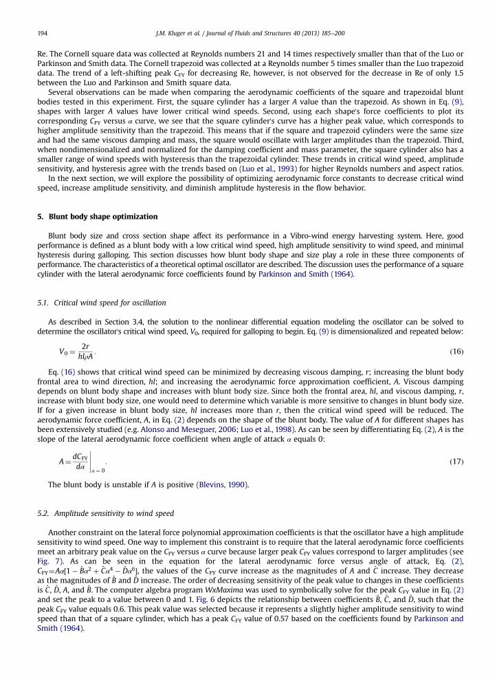
Another constraint on the lateral force polynomial approximation coefficients is that the oscillator have a high amplitudesensitivity to wind speed. One way to implement this constraint is to require that the lateral aerodynamic force coefficientsmeet an arbitrary peak value on the CFY versus α curve because larger peak CFY values correspond to larger amplitudes (seeFig. 7). As can be seen in the equation for the lateral aerodynamic force versus angle of attack, Eq. (2),CFY¼Aα½1� Bα2 þ Cα4 � Dα6�, the values of the CFY curve increase as the magnitudes of A and C increase. They decreaseas the magnitudes of B and D increase. The order of decreasing sensitivity of the peak value to changes in these coefficientsis C, D, A, and B. The computer algebra program WxMaxima was used to symbolically solve for the peak CFY value in Eq. (2)and set the peak to a value between 0 and 1. Fig. 6 depicts the relationship between coefficients B, C, and D, such that thepeak CFY value equals 0.6. This peak value was selected because it represents a slightly higher amplitude sensitivity to windspeed than that of a square cylinder, which has a peak CFY value of 0.57 based on the coefficients found by Parkinson andSmith (1964).

010

2030

4050

6070

0500

10001500

20002500

C/A

B/A

D/A

106

105

104

103

102

101

Region 2:peak CFY<0.6,

Hysteresis

Region 1:peak CFY<0.6,No Hysteresis

Region 3:peak CFY>0.6,

Hysteresis

Region 4 (in between surfaces):peak CFY>0.6,No Hysteresis

Fig. 6. Three-dimensional plot of surfaces with no hysteresis and a desired maximum CFY value. Increasing the assumed A value of the peak CFY surfaceshifts it upwards along the D/A axis. , peak CFY surface: Surface for which the peak value of the CFY curve is 0.6 and A is 2.69. , no hysteresissurface: Surface for which hysteresis has been eliminated. ■, square (Parkinson and Smith, 1964); ●, Cornell Trapezoid (see Table 2); Δ, coefficients baseddirectly on Luo et al.'s (1993) data for a triangle (η¼ 0): Overrepresented peak CFY value (A¼2.0). ○, Luo trend, 0.1≤η≤0.7, and 0.8≤η≤0.9: Skewed depictionrelative to peak CFY surface. ◊, Coefficients directly based on Luo et al.'s (1993) data for a trapezoid: η¼ 0.5: Overrepresented peak CFY value (A¼1.6). ★, Luotrend: η¼0.7. , Luo trend: 0.7oηo0.8. , Luo et al.'s (1993) trend: η¼0.8. ◆, Coefficients directly based on Luo et al.'s (1993) data: η¼0.75. , Luotrend: η¼0.9: Underrepresented peak CFY value (A¼4.2).

J.M. Kluger et al. / Journal of Fluids and Structures 40 (2013) 185–200 195

5.3. Hysteresis minimization

The final constraint on the lateral aerodynamic force approximation coefficients is that the oscillator exhibit minimalhysteresis. This requirement is imposed because practical wind energy harvesting will occur in a variable windenvironment, and with hysteresis, one would not know which bifurcation branch the oscillator would end up on. It isbetter to minimize hysteresis and eliminate it if possible.

For this purpose, we solved Eq. (7) for the starting and ending wind speeds of the hysteresis region as a function of theoscillator parameters. We did this using the computer algebra program WxMaxima. First, we set the derivative of Eq. (7)with respect to Y equal to 0. This equation was then combined with Eq. (7) in order to eliminate Y . The final equation is aquadratic on U, and its two roots are the nondimensionalized wind speeds for which hysteresis begins and ends (i.e. thelocal extrema in Fig. 2 for U(Y)). Using the quadratic formula on the final equation, the nondimensionalized wind speedswhen hysteresis starts and ends obey the following equation:

UHysteresis ¼ð13230D2

−3780BCDþ 800C3Þζ 7ζ

ffiffiffiffiffiffiffiffiffiffiffiffiffiffiffiffiffiffiffiffiffiffiffiffiffiffiffiffiffiffiffiffiffiffiffiffiffi80ð20C2

−63BDÞ3q

nAð6615D2−3780BCDþ 800C

3 þ 756B3D−180B

2C2Þ

; ð18Þ

where ζ is the reduced damping coefficient, n is the mass parameter, and A, B, C, and D, are the lateral force coefficients.The hysteresis region is eliminated when the discriminant of Eq. (18) is equal to or less than 0. When the discriminant

equals 0, the starting and ending wind speeds equal each other, and the local maximum and minimum in the curve of Uversus Y (as shown in Fig. 8) become a single inflection point. The discriminant equals 0 and hysteresis vanishes when

BD

C2 ≥0:318: ð19Þ

2 4 6 8 10 12 14 16 18 200

0.5

1

1.5

2

2.5

3

Nondimensionalized Wind Speed, U

Non

dim

ensi

onal

ized

Am

plitu

de, Y

0 5 10 15 20 25 300

0.2

0.4

0.6

0.8

1

1.2

1.4

1.6

1.8

angle of attack, � (deg)

Lat

eral

For

ce C

oeff

icie

nt, C

FY

Fig. 7. (Top) CFY versus α for blunt bodies with force coefficients in different regions of Fig. 6. (Bottom) The corresponding nondimensionalized amplitudeversus wind speed diagrams for parameter values of natural frequency, ω¼ 108 rad/s, damping coefficient, ζ¼0.0095, and mass parameter, n¼1.4e−3.— Region 1: A¼2.69, B¼ 17.6, C¼ 391, D¼ 6.00e3. — ∙ — Region 2: square cylinder (Parkinson & Smith, 1964): A¼2.69, B¼ 62.5, C¼2330, D¼ 2.3e4. ∙∙∙∙∙Region 3: A¼2.69, B¼17.6, C¼ 391, D¼1.65e3. ———— Region 4: A¼2.69, B¼3.65, C¼62.5, D¼397. ———— Region 4 when larger A value: A¼5.38, B¼3.65,C¼ 62.5, D¼397.

J.M. Kluger et al. / Journal of Fluids and Structures 40 (2013) 185–200196

The findings from this analysis are that the existence of hysteresis depends only on the parameters B, C, and D, for anyoscillator.

When the hysteresis region does exist, values of parameters in Eq. (18) affect its size and location. For typical forcecoefficient values, increasing the magnitude of B or D shifts the hysteresis region to higher wind speeds and decreases therange of wind speeds with hysteresis. Increasing the magnitude of C shifts the hysteresis region to lower wind speeds andincreases the range of wind speeds with hysteresis. B, C, and D values can be changed by altering a blunt body's shape.

According to Eq. (18), the midpoint and range of nondimensional wind speeds in the hysteresis region are bothproportional to the nondimensional group ζ/nA, or (reduced damping coefficient)/(mass parameter x A). When this expressionis dimensionalized, the midpoint and range of wind speeds in the hysteresis region are proportional to r/hl, where r is theviscous damping, and hl is the blunt body's frontal area to the wind direction. Thus, the location and size of the hysteresisregion can be adjusted by changing the blunt body shape (which changes A and viscous damping) or its size (which changesfrontal area and viscous damping). Additional significance to the hysteresis midpoint and range both being proportional toζ/nA is that changing a parameter in this group can reduce hysteresis and shift it to lower wind speeds, or increase hysteresisand shift it to higher wind speeds. However, such a change cannot both decrease the size of the region and shift it to higherwind speeds. Also, since the expression ζ/nA is the same nondimensional group that appears in the expression for criticalwind speed (see Eq. (9)), adjusting these parameters to shift the hysteresis region also shifts the critical wind speed by aproportional amount. Furthermore, the expression ζ/nA is independent of oscillator natural frequency, or, its mass andcantilever stiffness, which signifies that changing the oscillator natural frequency does not affect the hysteresis region orcritical wind speed.

0 0.2 0.4 0.6 0.8 11

2

3

4

5

6

η η

η η

Coe

ffici

ent V

alue

0 0.2 0.6 0.8 10

10

20

30

40

50

Coe

ffici

ent V

alue

0 0.2 0.4 0.6 0.8 10

200

400

600

800

1000

1200

1400

Coe

ffici

ent V

alue

0 0.2 0.4 0.6 0.8 10

2000

4000

6000

8000

10000

12000

14000

Coe

ffici

ent V

alue

Experimental Value

Experimental ValueB = -6.3η + 1.5e3.1η

α

U

h

h3h/4h/

2

Experimental ValueD = 2,300η + 6.4*10-5e19η

Experimental ValueC = -380η + 75e1.8η

0.4

A = -6.6η + 2.0e1.8η

^

^

^

^

^

^

Fig. 8. Trends in lateral force coefficients as η, the ratio of rear diameter:front diameter, changes from 0 to 1, where η¼0 represents a triangle and η¼1represents a square. Fractional η's represent trapezoids. The data shown here supports the concept of a continuum of aerodynamic force coefficientscorresponding to varying shape dimensions. These force coefficients are based on data collected by Luo et al. (1993) for blunt bodies with cross sectiondimensions shown in the center image. These shapes include —, square;————, trapezoid 1; — ∙ —, trapezoid 2; ∙∙∙∙∙, triangle, for which d¼50 mm.

J.M. Kluger et al. / Journal of Fluids and Structures 40 (2013) 185–200 197

5.4. Findings relating geometry to performance

The three subsections above describe how blunt body cross sectional shape affects the oscillator's critical wind speed,amplitude sensitivity to wind speed, and hysteresis region. If one assumes a continuum of shapes corresponding to acontinuous variation of constants A, B, C, and D, then one can search in this design space for shapes that satisfy the threedesign criteria. Evidence of a such a continuum is discussed in Section 5.4.1. Fig. 6 shows values of B, C, and D in B-C-D- spacethat eliminate hysteresis or satisfy the peak CFY requirement.

As shown in Fig. 6, the lateral force coefficients of a blunt body can fall into one of four regions. Regions above the peakCFY surface have lower amplitude sensitivity while regions below the surface have higher amplitude sensitivity. Regionsabove the No Hysteresis surface do not have a hysteresis region while regions below the surface do have a hysteresis region.Therefore, the optimal blunt body lies in the region above the No Hysteresis surface and below the peak CFY surface. Althoughnot clearly visible in the figure, a small optimal region occurs after the surfaces cross for small B, C, and D values. This regionis labeled as Region 4. Fig. 7 plots the CFY versus α curves and Y versus U curves for blunt bodies in each region.

The spatial relationship of these two surfaces depicts a general trade-off between large amplitude sensitivity andminimal hysteresis. This trade-off is supported mathematically. As discussed in Section 5.2 and shown in Eq. (2),CFY¼Aα½1−Bα2 þ Cα4−Dα6�; the peak CFY value of a blunt body increases if the magnitudes of A and C increase anddecreases if the magnitudes of B and D increase. This means that for a blunt body with a given A value, larger peak CFY valuesoccur for smaller ratios of BD : C

2. On the other hand, Eq. (19) shows that hysteresis is eliminated for BD=C

2≥0:318. That is,

hysteresis is minimized for larger ratios of BD : C2. As shown in Eqs. (2) and (18), larger A values both increase the peak CFY

value and minimize the size of the hysteresis region. For an A value of 2.69, relatively small B, C, and D values satisfy therequirements for large amplitude sensitivity and minimal hysteresis, as indicated by Region 4 in Fig. 6. In this optimalregion, BD=C

2is only slightly larger than 0.318 so that hysteresis is just eliminated and the peak CFY value is just above 0.6.

The location of the peak CFY surface in this figure depends on both the arbitrary peak value desired for the CFY versus αcurve and the assumed value of A (Fig. 6 assumes a value of A because there are four force coefficients, but only three axes

J.M. Kluger et al. / Journal of Fluids and Structures 40 (2013) 185–200198

may be drawn.). As shown in Eq. (2), CFY ¼ Aα½1� Bα2 þ Cα4 � Dα6�, the peak value of the CFY versus α curve is directlyproportional to A when all other coefficients stay constant. Increasing the assumed value of A while keeping the desiredpeak CFY value constant would make the peak CFY surface appear to shift upwards along the D axis, increasing the size of theoptimal Region 4. Effectively, if A increases, then B must increase, C must decrease, or D must increase to satisfy the peakvalue. Conversely, the effect of increasing the desired peak CFY value while keeping the assumed value of A constant is toshift the peak CFY surface downwards.

Fig. 6 shows the peak CFY surface for a peak CFY value of 0.6 and an A value of 2.69. For the reasons described in theprevious paragraph, the peak CFY surface is inaccurately plotted relative to the experimental B, C, and D values if theexperimental A values greatly differ from the assumed A value of the peak CFY surface. A¼ 2.69 was chosen for the peak CFYsurface in Fig. 6 because that is the approximate A value for the Parkinson and Smith square blunt body, Cornell trapezoid,and Luo trapezoid 1 (see Tables 1 and 2).

The coefficients for the square cylinder found by Parkinson and Smith (1964) lie below the No Hysteresis and above thepeak CFY surface, in Region 2. That is, the square cylinder has a low amplitude sensitivity and a hysteresis region. Coefficientsfor all other shapes and experimental conditions described in this paper fall in Region 3, which has a higher amplitudesensitivity than Region 2 but also exhibits hysteresis. These shapes include two trapezoidal cylinders with rear:frontdiameter ratios, η, of 0.75 as listed in Table 2. They also include a trapezoidal cylinder with η¼ 0.5 and a triangle (η¼ 0)based on data collected by Luo et al. (1993) that is discussed in Section 5.4.1. Fig. 6 slightly overrepresents the distances ofthese two shapes from the peak CFY surface, meaning that Fig. 6 implies larger peak CFY values, because the shapes' actual Avalues are less than the assumed A value of the peak CFY surface. Although all in Region 3, some of these shapes, such as theCornell trapezoid, are closer to the optimal Region 4 than others.

Fig. 6 also plots the trend in B, C, and D values suggested by Luo et al.'s (1993) data as a blunt body cross sectiontransitions from a triangle to a square. This trend is discussed in detail in Section 5.4.1. The A values of this trend are within10% of 2.69 for 0.7≤η≤0.8, where η is the ratio of the cross sectional rear:front diameter as shown in Fig. 8. Therefore, thedepiction of this trend with respect to the peak CFY surface in Fig. 8 is fairly accurate for these values of η. For plottedsegments of the trend corresponding to 0.1≤η≤0.7 and 0.8≤η≤0.9, A(η) differs by more than 10% from 2.69, and Fig. 6 skewsthe quantitative relationship of the trend's coefficients with respect to the peak CFY surface. For η¼ 0.1, Fig. 6 overrepresentsthe peak CFY value by 55%. For η¼ 0.9, Fig. 6 underrepresents the peak CFY value by 35%. However, these data points areincluded because they accurately depict the suggested qualitative performance of the trend.

In addition to suggesting the blunt body geometry for improved energy harvester performance, the trends in lateralaerodynamic force coefficients fitted to Luo's data support the idea that there is a continuum of shapes corresponding togradual variations in constants A, B, C, and D and that one can search in this design space for shapes that satisfy the threedesign criteria (Luo et al., 1993). Experimental studies supporting the shape continuum concept are described in the nextsection.

5.4.1. Data supporting a continuum of lateral force coefficientsThe previous section describes aerodynamic force approximation coefficients that minimize hysteresis and satisfy

amplitude sensitivity to wind speed. That discussion assumes that continuously changing a blunt body shape continuouslychanges its aerodynamic force coefficients. Here, previous experimental studies that describe the coefficients of graduallyadjusted blunt body shapes are shown to support this continuum concept. These studies also suggest which shapes in thecontinuum have optimal coefficient values.

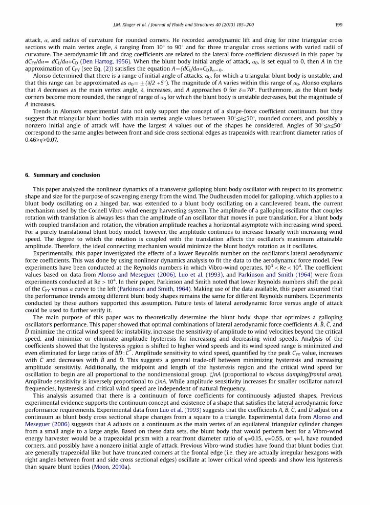
Luo et al. (1993) measured the lateral aerodynamic force coefficient, CFY, versus angle of attack, α, for blunt bodies withincrementally decreased rear diameters (see Fig. 8). The four shapes tested by Luo occupy a parameter space in which asquare is at one extreme, a triangle is at the other extreme, and two trapezoids are intermediate shapes. The data collectedby Luo can be fitted to the polynomial, CFY ¼ Aα½1−Bα2 þ Cα4−Dα6�. Fig. 8 shows how the coefficients in this equation variedfor each shape. The force coefficients for increasing rear diameter:front diameter ratio, η, in Fig. 8 can be fitted to functionsthat sum one linear and one exponential term. The way in which these experimental coefficients seem to follow a patternsuggests that a coefficient-shape continuum does exist and can be exploited to optimize blunt body performance.

Luo's studies have shown that different blunt body shapes are unstable for different ranges of α, have different peak CFYvalues, and show varying amounts of hysteresis (Luo et al., 1993, 1998). His data shows that the range of α for which theblunt body is unstable (that is, dCFY/dα40) increases as the cylinder becomes less square (that is, η decreases). It also showsthat hysteresis tends to decrease and the peak CFY value tends to increase as η decreases. As discussed in Section 5.2, largerpeak CFY values correlate to larger blunt body amplitudes for a given wind speed.

The trends fitted to Luo's data in Fig. 8 suggest that for 0oηo0.15 and 0.6oηo1, cylinders have high amplitudesensitivity and exhibit hysteresis. Since A is larger for η40.6, these cylinders also have lower critical wind speeds.Additionally, although cylinders for η40.85 have hysteresis, the amount of hysteresis decreases as η increases. For,0.15≤η≤0.6, cylinders have lower amplitude sensitivity and no hysteresis. The trade-off between higher amplitudesensitivity or less hysteresis, as discussed in Section 5.4, makes the optimal cylinders occur for the η values in whichhysteresis has just disappeared (that is, BD=C

2 ¼ 0:318). Such η values include η¼ 0.15, η¼0.6, and η¼1. Since the value of Ais larger for η≥0.6, the optimal rear:front diameter values may be η¼0.6 or η≈1, which represent square-like trapezoids.

Further evidence supporting a continuum of shape coefficients is provided by Alonso and Meseguer (2006). Alonso hasexperimentally determined trends in the instability of isosceles triangle blunt bodies for varied main vertex angle, δ, angle of

J.M. Kluger et al. / Journal of Fluids and Structures 40 (2013) 185–200 199

attack, α, and radius of curvature for rounded corners. He recorded aerodynamic lift and drag for nine triangular crosssections with main vertex angle, δ ranging from 101 to 901 and for three triangular cross sections with varied radii ofcurvature. The aerodynamic lift and drag coefficients are related to the lateral force coefficient discussed in this paper bydCFY/dα¼ dCL/dα+CD (Den Hartog, 1956). When the blunt body initial angle of attack, α0, is set equal to 0, then A in theapproximation of CFY (see Eq. (2)) satisfies the equation A¼(dCL/dα+CD)|α¼0.

Alonso determined that there is a range of initial angle of attacks, α0, for which a triangular blunt body is unstable, andthat this range can be approximated as α0¼7(δ/2 +51). The magnitude of A varies within this range of α0. Alonso explainsthat A decreases as the main vertex angle, δ, increases, and A approaches 0 for δ¼701. Furthermore, as the blunt bodycorners become more rounded, the range of range of α0 for which the blunt body is unstable decreases, but the magnitude ofA increases.

Trends in Alonso's experimental data not only support the concept of a shape-force coefficient continuum, but theysuggest that triangular blunt bodies with main vertex angle values between 301≤δ≤501, rounded corners, and possibly anonzero initial angle of attack will have the largest A values out of the shapes he considered. Angles of 301≤δ≤501correspond to the same angles between front and side cross sectional edges as trapezoids with rear:front diameter ratios of0.46≥η≥0.07.

6. Summary and conclusion

This paper analyzed the nonlinear dynamics of a transverse galloping blunt body oscillator with respect to its geometricshape and size for the purpose of scavenging energy from the wind. The Oudheusden model for galloping, which applies to ablunt body oscillating on a hinged bar, was extended to a blunt body oscillating on a cantilevered beam, the currentmechanism used by the Cornell Vibro-wind energy harvesting system. The amplitude of a galloping oscillator that couplesrotation with translation is always less than the amplitude of an oscillator that moves in pure translation. For a blunt bodywith coupled translation and rotation, the vibration amplitude reaches a horizontal asymptote with increasing wind speed.For a purely translational blunt body model, however, the amplitude continues to increase linearly with increasing windspeed. The degree to which the rotation is coupled with the translation affects the oscillator's maximum attainableamplitude. Therefore, the ideal connecting mechanism would minimize the blunt body's rotation as it oscillates.

Experimentally, this paper investigated the effects of a lower Reynolds number on the oscillator's lateral aerodynamicforce coefficients. This was done by using nonlinear dynamics analysis to fit the data to the aerodynamic force model. Fewexperiments have been conducted at the Reynolds numbers in which Vibro-wind operates, 103oReo104. The coefficientvalues based on data from Alonso and Meseguer (2006), Luo et al. (1993), and Parkinson and Smith (1964) were fromexperiments conducted at Re4104. In their paper, Parkinson and Smith noted that lower Reynolds numbers shift the peakof the CFY versus α curve to the left (Parkinson and Smith, 1964). Making use of the data available, this paper assumed thatthe performance trends among different blunt body shapes remains the same for different Reynolds numbers. Experimentsconducted by these authors supported this assumption. Future tests of lateral aerodynamic force versus angle of attackcould be used to further verify it.

The main purpose of this paper was to theoretically determine the blunt body shape that optimizes a gallopingoscillator's performance. This paper showed that optimal combinations of lateral aerodynamic force coefficients A, B, C, andD minimize the critical wind speed for instability, increase the sensitivity of amplitude to wind velocities beyond the criticalspeed, and minimize or eliminate amplitude hysteresis for increasing and decreasing wind speeds. Analysis of thecoefficients showed that the hysteresis region is shifted to higher wind speeds and its wind speed range is minimized andeven eliminated for large ratios of BD : C

2. Amplitude sensitivity to wind speed, quantified by the peak CFY value, increases

with C and decreases with B and D. This suggests a general trade-off between minimizing hysteresis and increasingamplitude sensitivity. Additionally, the midpoint and length of the hysteresis region and the critical wind speed foroscillation to begin are all proportional to the nondimensional group, ζ/nA (proportional to viscous damping/frontal area).Amplitude sensitivity is inversely proportional to ζ/nA. While amplitude sensitivity increases for smaller oscillator naturalfrequencies, hysteresis and critical wind speed are independent of natural frequency.

This analysis assumed that there is a continuum of force coefficients for continuously adjusted shapes. Previousexperimental evidence supports the continuum concept and existence of a shape that satisfies the lateral aerodynamic forceperformance requirements. Experimental data from Luo et al. (1993) suggests that the coefficients A, B, C, and D adjust on acontinuum as blunt body cross sectional shape changes from a square to a triangle. Experimental data from Alonso andMeseguer (2006) suggests that A adjusts on a continuum as the main vertex of an equilateral triangular cylinder changesfrom a small angle to a large angle. Based on these data sets, the blunt body that would perform best for a Vibro-windenergy harvester would be a trapezoidal prism with a rear:front diameter ratio of η≈0.15, η≈0.55, or η≈1, have roundedcorners, and possibly have a nonzero initial angle of attack. Previous Vibro-wind studies have found that blunt bodies thatare generally trapezoidal like but have truncated corners at the frontal edge (i.e. they are actually irregular hexagons withright angles between front and side cross sectional edges) oscillate at lower critical wind speeds and show less hysteresisthan square blunt bodies (Moon, 2010a).

J.M. Kluger et al. / Journal of Fluids and Structures 40 (2013) 185–200200

References

Alonso, G., Meseguer, J., 2006. A parametric study of the galloping stability of two-dimensional triangular cross section bodies. Journal of Wind Engineeringand Industrial Aerodynamics 94, 241–253.

Barrero-Gil, A., 2010. Energy harvesting from transverse galloping. Journal of Sound and Vibration 329, 2873–2883.Barrero-Gil, A., Sanz-Andrés, A., Alonso, G., 2009. Hysteresis in transverse galloping: the role of the inflection points. Journal of Fluids and Structures 25,

1007–1020.Blevins, R.D., 1990. In: Flow-Induced Vibration, second ed. Van Nostrand Reinhold, New York.Bryant, M., Garcia, E., 2011. Modeling and testing of a novel aeroelastic flutter energy harvester. Journal of Vibration and Acoustics 133, 011010.Den Hartog, J.P., 1956. In: Mechanical Vibrations, fourth ed. McGraw-Hill, New York.Erturk, A., Vieira, W.G.R., De Marqui Jr., C., Inman, D.J., 2010. On the energy harvesting potential of piezoaeroelastic systems. Applied Physics Letters 96,

184103.Frayne, S.M., 2008. Generator Utilizing Fluid-Induced Oscillations. United States of America, Patent No. US2008129254.Inman, D.J., 2008. In: Engineering Vibration, third ed. Pearson Prentice Hall, Upper Saddle River, N.J.Kuroda, M., Moon, F.C., 2007. Experimental reconsideration of spatio-temporal dynamics observed in fluid-elastic oscillator arrays from a complex system

point of view. Journal of Complexity 12, 36–47.Li, S., Lipson, H., 2009. Vertical-stalk flapping-leaf generator for parallel wind energy harvesting. In: Proceedings of AMSE/AIAA Conference on Smart

Materials and Adaptive Structures. Oxnard, California, pp. 1276.Luo, S.C., Chew, Y.T., Ng, Y.T., 2003. Hysteresis phenomenon in the galloping oscillation of a square cylinder. Journal of Fluids and Structures. 18, 103–118.Luo, S.C., Chew, Y.T., Yazdani, M.G., 1998. Stability to translational galloping vibration of cylinders at different mean angles of attack. Journal of Sound and

Vibration 215, 1183–1194.Luo, S.C., Yazdani, M.G., Chew, Y.T., Lee, T.S., 1993. Effects of incidence and afterbody shape on flow past bluff cylinders. Journal of Wind Engineering and

Industrial Aerodynamics. 53, 375–399.McKinney, W., DeLaurier, J.D., 1981. Wingmill-an oscillating-wing windmill. Energy 5, 109–115.Moon, F., 1992. Chaotic and Fractal Dynamics: an Introduction for Applied Scientists and Engineers. Wiley, New York.Moon, F.C., 2010a. Principles of Nonlinear Vibro-Wind Energy Conversion. In: Hutter, K., Wu, T., Shu, Y. (Eds.), FromWaves in Complex Systems to Dynamics

of Generalized Continua, World Scientific, Hackensack, New Jersey, pp. 385–401.Moon, F.C., 2010b. Vibro-wind energy technology for architectural applications. Accessed 4/28/2013 ⟨http://www.windtech-international.com/articles/

vibro-wind-energy-technology-for-architectural-applications⟩.Novak, M., ASCE, M., Tanaka, H., 1974. Effect of turbulence on galloping instability. ASCE Journal of the Engineering Mechanics Division 100, 27–47.Parkinson, G.V., Smith, J.D., 1964. The square prism as an aeroelastic non-linear oscillator. The Quarterly Journal of Mechanics and Applied Mathematics 17,

225–239.Rand, R.H., 2012. Lecture Notes on Nonlinear Vibrations. Accessed 8/15/2012 ⟨http://ecommons.library.cornell.edu/handle/1813/28989⟩.Rand, R.H., Armbruster, D., 1987. Perturbation Methods, Bifurcation Theory, and Computer Algebra. Springer-Verlag, New York.Tang, L., Paidoussis, M.P., DeLaurier, J.D., 2008. Flutter-Mill: A New Energy-Harvesting Device. Accessed 8/15/2012 ⟨http://64.34.71.154/Storage/26/

1817_Flutter-Mill-_a_New_Energy-Harvesting_Device.pdf⟩.Van Oudheusden, B.W., 1995. On the quasi-steady analysis of one-degree-of-freedom galloping with combined translational and rotational effects.

Nonlinear Dynamics 8, 435–451.