journal of monetary economics - matteo iacoviello

Contents lists available at ScienceDirect

Journal of Monetary Economics

Journal of Monetary Economics 70 (2015) 22–38

http://d0304-39

n CorrE-m1 Te2 Th

methodof consu

3 Odiscrete

journal homepage: www.elsevier.com/locate/jme

OccBin: A toolkit for solving dynamic models withoccasionally binding constraints easily

Luca Guerrieri a,n, Matteo Iacoviello b,1

a Office of Financial Stability, Federal Reserve Board, 20th and C Streets NW, Washington, DC 20551, United Statesb Division of International Finance, Federal Reserve Board, 20th and C Streets NW, Washington, DC 20551, United States

a r t i c l e i n f o

Article history:Received 19 July 2013Received in revised form12 August 2014Accepted 14 August 2014Available online 6 September 2014

Keywords:Occasionally binding constraintsDSGE modelsRegime shiftsFirst-order perturbation

x.doi.org/10.1016/j.jmoneco.2014.08.00532/Published by Elsevier B.V.

esponding author. Tel.: þ1 202 452 2550.ail addresses: [email protected] (L. Guerl.: þ1 202 452 2426.e virtually exact solution is obtained eithers, following Christiano and Fisher (2000). Inmption choice subject to a constraint on bour approach, including the title of this paper,-time stochastic models without occasionall

a b s t r a c t

The toolkit adapts a first-order perturbation approach and applies it in a piecewise fashionto solve dynamic models with occasionally binding constraints. Our examples include areal business cycle model with a constraint on the level of investment and a NewKeynesian model subject to the zero lower bound on nominal interest rates. Comparedwith a high-quality numerical solution, the piecewise linear perturbation method canadequately capture key properties of the models we consider. A key advantage of thepiecewise linear perturbation method is its applicability to models with a large number ofstate variables.

Published by Elsevier B.V.

1. Introduction

Inequality constraints that bind occasionally arise in a wide array of economic applications. We describe how to adapt afirst-order perturbation approach and apply it in a piecewise fashion to handle occasionally binding constraints. Toshowcase the applicability of our approach, we solve two popular dynamic stochastic models. The first model is an RBCmodel with limitations on the mobility of factors of production. The second model is a canonical New Keynesian modelsubject to the zero lower bound on nominal interest rates. As is typical for dynamic models, the models we consider do nothave a closed-form analytical solution. In each case, we compare the piecewise linear perturbation solution with a high-quality numerical solution that can be taken to be virtually exact.2

Our contribution is twofold. First, we outline an algorithm to obtain a piecewise linear solution. While the individualelements of the algorithm are not original, our recombination simplifies the application of this type of solution to a generalclass of models.3 We offer a library of numerical routines, OccBin, that implements the algorithm and is compatible withDynare, a convenient and popular modeling environment (Adjemian et al., 2011). Second, we present a systematicassessment of the quality of the piecewise linear perturbation method relative to a virtually exact solution, which has notbeen attempted by others. Because standard perturbation methods only provide a local approximation, they cannot capture

rieri), [email protected] (M. Iacoviello).

by dynamic programming on a very fine lattice for the state variables of the model or by spectraladdition to the RBC and New Keynesian models, an online appendix evaluates our solution for a modelrrowing.is inspired by the work by Uhlig (1995) who developed an early toolkit to analyze nonlinear dynamicy binding constraints.

www.sciencedirect.com/science/journal/03043932

www.elsevier.com/locate/jme

http://dx.doi.org/10.1016/j.jmoneco.2014.08.005



http://crossmark.crossref.org/dialog/?doi=10.1016/j.jmoneco.2014.08.005&domain=pdf



mailto:[email protected]

mailto:[email protected]


L. Guerrieri, M. Iacoviello / Journal of Monetary Economics 70 (2015) 22–38 23

occasionally binding constraints without adaptation. Our analysis builds on an insight that has been used extensively in theliterature on the effects of attaining the zero-lower bound on nominal interest rates.4 That insight is that occasionallybinding constraints can be handled as different regimes of the same model. Under one regime, the occasionally bindingconstraint is slack. Under the other regime, the same constraint is binding. The piecewise linear solution method involveslinking the first-order approximation of the model around the same point under each regime. Importantly, the solution thatthe algorithm produces is not just linear – with two different sets of coefficients depending on whether the occasionallybinding constraint is binding or not – but rather, it can be highly nonlinear. The dynamics in one of the two regimes maycrucially depend on how long one expects to be in that regime. In turn, how long one expects to be in that regime dependson the state vector. This interaction produces the high nonlinearity.

Our assessment focuses on several aspects of the solution. Following Christiano and Fisher (2000), we compare momentsof key variables by reporting mean, standard deviation, and skewness. Following Taylor and Uhlig (1990), we compare plotsof stochastic simulations. In addition, we assess the accuracy of the piecewise linear approximation by computing twobounded rationality metrics. The first metric is the Euler equation residual, following Judd (1992). The Euler equationresidual quantifies the error in the intertemporal allocation problem using units of consumption. The second metric relieson the broader evaluation of expected utility. Intuitively, the closest approximation to the solution of the model will lead tothe highest utility level. The difference in utility implied by two solution methods can also be expressed as a compensatingvariation in consumption that a utility-maximizing agent would have to be offered in order to continue using the lessaccurate method. On the basis of these comparisons and assessments, we find that the piecewise linear perturbationmethod can capture adequately key properties of the models we consider.

We also highlight some limitations of the piecewise linear solution. Namely, just like any linear solution, it discards allinformation regarding the realization of future shocks. Accordingly, our piecewise linear approach is not able to captureprecautionary behavior linked to the possibility that a constraint may become binding in the future, as a result of shocks yetunrealized. However, the piecewise method also inherits some of the key advantages of a first-order perturbation approach.It is computationally fast and applicable to models with a large number of state variables even when the curse ofdimensionality renders other higher-quality methods inapplicable.5 Moreover, our library of numerical routines accepts amodel written in a natural way with no meaningful syntax restrictions. Accordingly, application of our algorithm to differentmodels requires only minimal programming.

Section 2 outlines the piecewise linear solution algorithm. Section 3 relates our approach to the literature. Section 4considers a real business cycle model with a constraint on investment. Section 5 considers a New Keynesian model subjectto the zero lower bound on nominal interest rates. Section 6 concludes.

2. The solution algorithm

For clarity of exposition, we confine our attention to a model with only one occasionally binding constraint. Extensions tomultiple occasionally binding constraints are implemented in the library of routines.

A model with an occasionally binding constraint is equivalent to one with two regimes. Under one regime, theoccasionally binding constraint is slack. Under the other regime, the constraint binds. We linearize the model under eachregime around the non-stochastic steady state, although a different point could be chosen. We dub the regime that appliesat the point of linearization the “reference” regime, or (M 1). We dub the other regime “alternative”, or (M 2). It is immaterialwhether the occasionally binding constraint is slack at the reference regime or at the alternative regime.

There are two important requirements for the application of our algorithm.

1.

of tillu

factfore

The conditions for existence of a rational expectations solution in Blanchard and Kahn (1980) hold at the referenceregime.

2.
If shocks move the model away from the reference regime to the alternative regime, the model will return to thereference regime in finite time under the assumption that agents expect that no future shocks will occur.6
2.1. Definition of a piecewise linear solution

Without loss of generality, when the occasionally binding constraint gðEtXtþ1;Xt ;Xt�1Þr0 is slack, the linearized systemof necessary conditions for an equilibrium under the reference regime can be expressed as

AEtXtþ1þBXtþCXt�1þEϵt ¼ 0; ðM1Þ

4 Recent examples of the use of this technique include Jung et al. (2005), Eggertsson and Woodford (2003), Christiano et al. (2011).5 The library of routines that accompanies this paper contains additional examples of models that can be solved with a piecewise linear algorithm. Onehe examples is the celebrated Smets and Wouters (2007) model, extended to incorporate the zero lower bound on the policy interest rate. As anstration of the speed of the piecewise linear algorithm, our toolkit solves that model in a fraction of a second.6 This restriction might appear draconian, but it is routinely imposed when solving DSGE models with standard first-order perturbation methods. In, the linear approximation to the solution could be equivalently characterized as implementing either the rational expectations restrictions or perfectsight.

L. Guerrieri, M. Iacoviello / Journal of Monetary Economics 70 (2015) 22–3824

where X is a vector of size n that collects all the endogenous variables; Et is the expectation operator, conditional oninformation available at time t; A, B, and C are n�n matrices of structural parameters for the model's linearized equationsthat are conformable with X; ϵ is a vector of zero mean, i.i.d. exogenous innovations of size m and E is an n�m matrix ofstructural parameters.

When the constraint binds, then hðEtXtþ1;Xt ;Xt�1Þ40. The analogous system of necessary conditions for an equilibriumunder the alternative regime, linearized again around the non-stochastic steady state, can be expressed as

AnEtXtþ1þBnXtþCnXt�1þDnþEnϵt ¼ 0: ðM2ÞThe matrices An, Bn, Cn are again n�n matrices of structural parameters. In addition, under (M2) there is a column vector ofparameters Dn whose size is n. The presence of Dn arises from the fact that the linearization is carried out around a point(the steady state by our choice) in which regime (M 1) applies. Finally En is another n�m matrix of structural parameters.Notice that the conditions implied by the functions g and h above are assumed to be mutually exclusive and collectivelyexhaustive. We are now in a position to define a solution for our model.

Definition 1. A solution for a model with an occasionally binding constraint is a function f :Xt�1 � ϵt-Xt such that theconditions under system (M 1) or the system (M 2) hold, depending on the evaluation of the occasionally binding constraint,governed by g and h.

An alternative way of characterizing the function f relies on matrix expressions which closely mirror the familiar decisionrules of a linearized dynamic model. Accordingly, given initial conditions X0 and the realization of a shock ϵ1, the function fcan be expressed as a set of matrices Pt , a set of matrices Rt , and a matrix Q1, such that

Xt ¼PtXt�1þRtþQ1ϵ1 for t ¼ 1 ð1Þ

Xt ¼PtXt�1þRt 8tAf2;1g: ð2ÞAs Eqs. (1) and (2) show, the solution from our piecewise algorithm need not be linear, even if the original system

described by (M 1) and (M 2) is. At each point in time the matrices Pt , Qt , Rt are time varying, even if they are functions ofXt�1 and ϵ1 only.

2.2. The solution algorithm

Given the conditions for an equilibrium in M 1 and M 2, and given the occasionally binding constraint expressed in g andh, the following algorithm characterizes the piecewise linear solution f, defined above. The output of the algorithm is a timevarying decision rule whose general form is given in Eqs. (1) and (2). Accordingly, the algorithm shows how to compute thematrices Pt , Qt , and Rt given initial conditions X0 and given the realization of a shock ϵ1.

The algorithm employs a guess-and-verify approach. First, we guess the periods in which each regime applies. Second,we proceed to verify and, if necessary, update the initial guess as follows:

1.
Let T be the date when the current guess implies that the model will return to regime (M 1). Then for any tZT , usingstandard perturbation methods, one can characterize the linear approximation to the decision rule for Xt, given Xt�1, as
Xt ¼PXt�1þQϵt ; ðM1DRÞwhere P and Q are n�n and n�m matrices of reduced-form parameters, respectively. Then, using the notation ofEquation (2), for any tZT , Pt ¼P, Rt ¼ 0.

2.
Using XT ¼PXT�1 and Equation (M 2), coupled with the assumption that agents expect no shocks beyond the first period,the solution in period T�1 will satisfy the following matrix equation:
AnPXT�1þBnXT�1þCnXT�2þDn ¼ 0: ð3ÞSolve the equation above for XT�1 to obtain the decision rule for XT�1, given XT�2:

XT�1 ¼ �ðAnPþBnÞ�1ðCnXT�2þDnÞ: ð4ÞAccordingly, PT�1 ¼ �ðAnPþBnÞ�1Cn and RT�1 ¼ �ðAnPþBnÞ�1Dn.

3.
Using XT�1 ¼PT�1XT�2þRT�1 and either (M 1) or (M 2), as implied by the current guess of regimes, solve for XT�2
given XT�3.
4. Iterate back in this fashion until X0 is reached, applying either (M 1) or (M 2) at each iteration, as implied by the current
guess of regimes.
5. Depending on whether regime (M 1) or (M 2) is guessed to apply in period 1, Q1 ¼ �ðAP2þBÞ�1E, or
Q1 ¼ �ðAnP2þBnÞ�1En. Trivially, in the special case in which regime (M 1) is guessed to apply in all periods, one cansee that Q1 ¼Q, consistent with equation (M 1DR).

6.
Using the guess for the solution obtained in steps 1 to 5, compute paths for X to verify the current guess of regimes. If theguess is verified, stop. Otherwise, update the guess for when regimes (M 1) and (M 2) apply and return to step 1.


0 1

solution to (M 1). In general, the guess will have to be updated, because a switch in regimes is associated with a change in
Given X and ϵ , an expedient initial guess of regimes can be obtained by applying the standard first-order perturbation
the paths of the endogenous variables. A choice for the updating scheme in step 6 that we have found resilient in practice isto use the path for X from the previous iteration to infer a new guess of regimes. As an alternative, one may choose todampen the iterations by shrinking (or expanding) the number of periods when a certain regime applies only gradually, in afashion analogous to the Gauss–Jacobi algorithm.

Computation of the solution requires a series of inversions for the matrix J t � ðAnPtþBnÞ, for t¼2 to t¼T. Contingent ona guess for a sequence of regimes, non-invertibility of the matrix J t implies the existence of multiple paths that lead backfrom the point XT to the point X0. In that case, the application of a pseudo-inverse, as suggested by Chen et al. (2012),arbitrarily selects one of these paths.

Notice that for multiple solutions to exist, non-invertibility of J t is neither sufficient nor necessary. It is not sufficientbecause one needs to also verify that the given guess of regimes is consistent with the occasionally binding constraint ofinterest after calculation of a full path for X. It is not necessary because distinct sequences of regimes may support multiplesolutions.

2.3. Implementation of the algorithm

The paper is complemented by a library of numerical routines, OccBin, that implements the piecewise linear solutionalgorithm using the MATLAB programming language. Our routines are designed as an add-on to Dynare, a widely used set ofprograms for the solution and estimation of DSGE models. Dynare lets users specify a DSGE model using a readable syntaxthat imposes only trivial requirements in the way a model is specified. The programs we devised take as inputs two Dynaremodel files. One file specifies the model (M 1) at the reference regime. The other file specifies the model at the alternativeregime (M 2). We use the analytical derivatives computed by Dynare to construct A;B; C; E;An;Bn; Cn;Dn, and En in equations(M 1) and (M 2). We also use the routines in Dynare to construct the matrices P and Q in equation (M 1DR).

2.4. Characteristics of the piecewise linear solution

A simple linear difference equation with an expectational term and a control term is an ideal vehicle to illustrate keycharacteristics of the piece-wise linear solution, before moving to a broader assessment of its performance for richermodels. Consider a variable q whose evolution is determined by the following schedule:

qt ¼ βð1�ρÞEtqtþ1þρqt�1�σrtþut ; ð5Þ

where Et is the conditional expectation operator, and β¼ 0:99, ρ¼ 0:5, and σ ¼ 5 are parameters. The current realization ofthe variable, qt, depends on its expectation for next period, and its value for the previous period. The variable also dependson the control term, rt, and an exogenous shock ut, which follows an AR(1) process with the autoregression coefficient of 0.5and a standard deviation of the innovation equal to 0.05. In turn, the control variable follows a simple feedback rule:

rt ¼maxðr;ϕqtÞ; ð6Þ

where ϕ¼ 0:2 is a parameter. The max operator prevents rt from falling below a certain lower bound chosen asr ¼ �ð1=β�1Þ. This system of difference equations has various economic interpretations.7 For concreteness, we interpretq as an asset price and r as a net policy interest rate (in deviation from its steady state of 1=β�1), subject to the zerolower bound.

The policy functions for qt and rt implied by the piecewise linear method are shown in Fig. 1. Starting from steady state,for realizations of the shock ut above a certain threshold, the decision rules are simply linear (and by construction there is nodifference with a linear solution). For realizations of ut above the threshold, higher values of ut lead to higher asset pricesand, through the feedback rule, higher interest rates.

When ut falls below the threshold, the feedback rule for the interest rate hits the lower bound constraint, and thepiecewise linear solution implies a switch in regimes. At this point, the policy functions depend on the expected duration ofthe lower-bound regime. Negative realizations of ut of larger magnitude imply a longer duration of the zero bound regime.In turn, this mechanism leads to a deeper decline in asset prices because the feedback rule is temporarily switched off. Theinset panel of Fig. 1 highlights that the slope of the decision rule is a step function. The different steps (slopes of the policyfunction for the asset price) correspond to different expected durations of the regime in which the lower bound on theinterest rate is enforced.

To underscore the value of concatenating the conditions for an equilibrium under different regimes, as implied by thepiecewise linear solution, it is useful to consider a “naive” piecewise linear solution scheme. Following this naive scheme, inorder to enforce the lower bound in Equation (6), we simply splice the decision rules for two models. The first rule is for amodel that excludes the lower bound at all times. The second rule is for a model that enforces the lower bound at all times.

7 See, for instance Chapter 5 of Blanchard and Fischer (1989).

−0.2 −0.15 −0.1 −0.05 0 0.05 0.1 0.15 0.2−1.5

−1

−0.5

0

0.5

1

1.5

2

2.5

3

3.5Policy Function for Interest Rate − Level

Per

cent

Piecewise LinearLinearNaive Piecewise LinearNonlinear

−0.2 −0.15 −0.1 −0.05 0 0.05 0.1 0.15 0.2−30

−20

−10

0

10

20

30

40

50

60

70Policy Function for Asset Price − Percent Dev. from Steady State

Per

cent

−0.2 0 0.20.5

1

1.5

2

2.5

Slope of Policy Function for Asset Pricefor the Piecewise Linear Solution

Shock

Fig. 1. Comparing the piecewise linear solution and a “naive” piecewise approach for a simple asset pricing model. Note: The values on the abscissaedenote shock sizes (for qt�1 ¼ 0). The “naive” solution is obtained by splicing two linearized decision rules obtained under the assumption that each regimeapplies indefinitely.


As Fig. 1 makes clear, the naive solution matches a linear solution for positive shocks that inflate the asset price. However,when negative shocks are large enough for the lower bound to be reached, the “naive” solution incorrectly implies that theconstraint will be enforced (and expected to be enforced) forever, only for those expectations to be dashed, even in theabsence of further shocks, once the interest rate eventually rises. Accordingly, the asset price jumps, rising closer to whatwould be an implied higher steady state, under the mistaken assumption that the regime will last forever. By contrast, underthe piecewise linear solution produced by OccBin, expectations reflect the duration of the lower bound regime, which avoidsthe large discontinuity in the policy function for asset prices. Accordingly, the policy functions retrieved by OccBin are muchcloser to the fully nonlinear policy functions from highly accurate projection methods.8

The fully nonlinear policy functions hug the policy functions obtained from our piecewise linear solution, but there aresome small differences. Shocks that move the interest rate close to its lower bound also imply that reaching the lower boundwill be more likely when additional shocks hit the asset pricing equation. This consideration is not incorporated in the policyfunctions for the piecewise linear solution. Accordingly, the interest rate and the asset price are slightly lower for largedeflationary shocks under the fully nonlinear solution than under the piecewise linear solution. Of course, just as thisanticipation of future regime switches is absent from the piecewise linear solution, it is also absent from the linear solutionand from the naive solution.

Finally, a further prosaic difference between the piecewise linear solution and the naive splicing of two linear decisionrules is the range of applicable models. The naive splicing can only be implemented when the Blanchard–Kahn conditionsapply separately to all regimes of interest. By contrast, for the piecewise linear solution, those conditions need not hold forthe alternative regime.

8 For the nonlinear solution we approximated the decision rule for the expectation of the asset price with a Chebyshev polynomial of order 6 andparameterized it with a standard collocation procedure. We approximated the AR(1) process for the shock ut with a Markov process with 51 states.


3. Related approaches

A recent review of solution algorithms that mitigate the curse of dimensionality, is provided by den Haan et al. (2011)and references therein. Judd et al. (2012) extend that review by considering methods appropriate for the solution of modelswith occasionally binding constraints. They do not dwell on piece-wise linear solutions. We do not attempt to replicate acomprehensive review of the literature but focus on the connection between the piecewise linear algorithm presentedabove and alternative algorithms that ameliorate the curse of dimensionality.

The idea of concatenating decision rules from multiple regimes and shooting back from the last period in which thereference regime is expected to apply in perpetuity can be traced back to Jung et al. (2005). Their focus is on an economysubject to the zero lower bound on nominal interest rates. Our formulation of the piecewise linear solution algorithmapplies to any linear model under a general form for the specification of the occasionally binding constraints.

One extension of the basic piecewise linear solution in Jung et al. (2005) is due to Eggertsson and Woodford (2003). Theyconsider a model with a shock to the natural rate of interest subject to a Markov process with only two states. In one state,the natural rate is so low that the zero lower bound binds. Under this stark stochastic structure, they compute a rationalexpectation solution, instead of a perfect-foresight solution. However, in their model the expected duration of thealternative regime, i.e. the policy rate at the lower bound, is always fixed at a value determined by the Markov process. Bycontrast, in our setup the duration of the alternative regime is dependent on the realization of shocks. In turn, theexpectation of how long a regime is expected to last affects the value of the endogenous variables contemporaneously.

Building on the work of Laséen and Svensson (2009), Holden and Paetz (2012) provide a solution method that allows foroccasionally binding constraints based on introducing anticipated shocks. With a first-order perturbation approach, theirmethod would produce paths for the endogenous variables identical to the ones of our piece-wise approach.9 The choice ofanticipated shocks that mimic occasionally binding constraints is specific to each model and is not amenable to a generalspecification, such as the one achieved for our algorithm.

Upon linearization of the model, an extended path algorithm, as the one proposed by Fair and Taylor (1983) and furtherdeveloped by Adjemian and Juillard (2011), would also yield the same path for the endogenous variables as our piecewiselinear algorithm. One advantage of the extended path algorithm is that it can also handle nonlinear perfect-foresightmodels, avoiding linearization altogether. However, in practice, convergence of the algorithm may be difficult without ahigh-quality initial guess. An advantage of our piecewise linear method is that it greatly simplifies the search process.Instead of searching for the paths of all the endogenous variables, the piecewise linear algorithm only needs to search for asequence of regimes.

The extended path algorithm relies on derivative-based methods to search for a solution. This search is complicated bythe fact that occasionally binding constraints introduce a discontinuity in the derivatives of the conditions for anequilibrium. Substitution of the kink implied by the occasionally binding constraint with a smooth polynomial approxima-tion may yield a reformulation of the model more easily amenable to derivative-based solution methods. Our attempts atpursuing this strategy revealed undesirable side effects. As we increased the order of the polynomial to get a betterapproximation to the kink implied by an occasionally binding constraint, the polynomial generated wild oscillations whenmoving away from the area immediately surrounding the kink.

An alternative way of masking the discontinuity implied by occasionally binding constraints is offered by McGrattan(1996), Preston and Roca (2007), and Kim et al. (2010). The insight is to penalize agents' utility when a particular constraintis hit. While this method has the advantage of converting a model with occasionally binding constraints into a model that issolvable by perturbation methods, it suffers from undesirable drawbacks. First, the solution will change with the size andthe shape of the penalty (the barrier parameter). Moreover, any high-order perturbation method will generate a smoothsolution that in some instances will violate the inequality constraint.

The remarkable recent work of Judd et al. (2012) also provides a solution algorithm that can handle both a sizablenumber of state variables and occasionally binding constraints. Their innovation is to use a simulation-based approach toconstruct the approximation grid for projection methods, which ameliorates the curse of dimensionality. However, thecomputational burden of this method may remain too high for models oriented towards empirical realism. For instance,Judd et al. (2012) highlight that a simplified version of the Smets–Wouters model with an added zero lower boundconstraint can be solved in 25 min (with serial processing in Matlab).

4. An RBC model with a constraint on investment

For its simplicity and widespread use, the RBC model is a staple of the literature that has compared the performance ofdifferent solution techniques (see for instance, Taylor and Uhlig, 1990). In our variant of this canonical model, the choice ofinvestment is subject to an occasionally binding constraint. This constraint prevents investment from falling below anexogenously fixed lower bound in every period. This exogenous lower bound could be set to imply that investment cannotbe negative. Accordingly, our model nests a model in which capital is irreversible.

9 An explanation for the equivalence of the two approaches and a discussion of their relative merits is provided in the appendices of Bodenstein et al.(2009, 2013).

Table 1Baseline calibration of RBC model with a constraint on investment.

Parameter Value

β, Discount factor 0.96δ, Depreciation rate 0.10ρ, Persistence of tech. shock 0.90ϕ, Threshold for investment constraint 0.975γ, Relative risk aversion 2α, Capital share 0.33σ, St. dev. of tech. innovation 0.013


4.1. Model overview

A central planner maximizes households' utility

max E0 ∑1

t ¼ 0βtC

1� γt �11�γ

;

subject to the constraints in Eqs. (7)–(9) below:

Ctþ It ¼ AtKαt�1; ð7Þ

Kt ¼ ð1�δÞKt�1þ It ; ð8Þ

ItZϕISS: ð9ÞThe planner chooses consumption, Ct, investment, It, and capital, Kt. Eq. (7) is the resource constraint and AtK

αt�1 is the

economy's output in period t. Technology At evolves according to

ln At ¼ ρ ln At�1þσϵt ; ð10Þwhere ρ and σ are parameters and ϵt is an exogenous innovation distributed as standard normal. Eq. (8) is the capitalaccumulation equation, with depreciation rate δ. Finally, Eq. (9) is an occasionally binding constraint that preventsinvestment from falling below a fraction ϕ of investment in the non-stochastic steady state, denoted by ISS. When theparameter ϕ equals 0, this last constraint implies that capital is irreversible. In the numerical experiments below, we set ϕ ata value well above zero which ensures that the constraint binds frequently.

Denoting with λt the Lagrange multiplier on the investment constraint given by (9), the equations describing thenecessary conditions for an equilibrium are (7), (8), and (10) together with the consumption Euler equation and the Kuhn–Tucker condition for the investment constraint:

C�γt �λt ¼ βEtðC�γ

tþ1ð1�δþαAtþ1Kα�1t Þ�ð1�δÞλtÞ ð11Þ

λtðIt�ϕISSÞ ¼ 0: ð12ÞThese equations form a dynamic system of five equations in the five variables fCt ; It ;Kt ;At ; λtg.

When mapping these conditions into the notation used in Section 2, (M 1) and (M 2) only differ because of one equationin this case. The complementary slackness condition for the optimization problem implies that λt ¼ 0 when the constraint isslack. Conversely, when the constraint binds, It ¼ϕISS. The conditions in (M 1) encompass λt ¼ 0 and the function g capturesItZϕISS. The conditions in (M 2) encompass It ¼ϕISS; and the function hcaptures λt40.

4.2. Calibration and policy functions

Table 1 summarizes the calibration, which reflects a choice of yearly frequency. Most parameter choices are standard. Therisk aversion parameter γ is set to 2: we discuss sensitivity to alternative choices below. We set ϕ¼ 0:975, which impliesthat the constraint binds about 40% of the time. We set α¼ 0:33, δ¼ 0:1, and β¼ 0:96. Finally, we set σ ¼ 0:013 and ρ¼ 0:9,these parameter choices imply a standard deviation of log output around 4 percent.

In the absence of an analytical closed-form solution for the model, we use projection methods and dynamicprogramming to characterize a high-quality, fully nonlinear solution.10 The resulting investment function of the fullnonlinear solution is shown in the top panel of Fig. 2. Regardless of the initial level of capital, low realizations of technologytrigger investment (in deviation from its steady state) to hit its lower bound given by �ð1�ϕÞ. The bottom panel comparesthe nonlinear solution to the piecewise solution obtained using our method. Given our benchmark calibration, investment isslightly lower under the piecewise solution when the irreversibility constraint does not bind. The higher level of investment

10 A detailed description of the algorithms for the fully nonlinear solution is given in Section A of the online appendix.

−3 −2.5 −2 −1.5 −1 −0.5 0 0.5 1 1.5 2 2.5−3

−2

−1

0

1

2

3

4

Technology, % from ss

Technology, % from ss

Inve

stm

ent,

% fr

om s

sIn

vest

men

t, %

from

ss

Investment function I(K,A), nonlinear solution, for different initial values of K

φ−1

K = 1.1 KSS

K = KSS

K = 0.975 KSS

−3 −2.5 −2 −1.5 −1 −0.5 0 0.5 1 1.5 2 2.5−3

−2

−1

0

1

2

3

4

Investment function, nonlinear vs piecewise solution

Nonlinear (K=KSS)

Piecewise (OccBin)

φ−1

Fig. 2. Policy function for investment, RBC model with a constraint on investment.


in the nonlinear solution comes from the effect of uncertainty on precautionary saving. However, the policy functions areremarkably close.

4.3. Assessing performance: impulse responses and moments

The transitional dynamics are illustrated in Fig. 3, which shows responses of the model variables to two shocks totechnology, the term ϵt in Eq. (10). The sizes of the two shocks are symmetric around the steady state. The first shock bringsdown the level of technology by 4 percent (close to a 3 standard deviation shock). The second shock pushes up the level oftechnology by 4 percent. For ease of comparison, responses to the first shock are shown on the left-hand side of the figure,and responses to the second shock on the right-hand side. In each column, the solid lines denote the piecewise linearsolution, the dashed lines denote the dynamic programming solution, and the dash-dotted lines denote the first-orderperturbation solution.

The decline in technology leads to a decline in investment large enough for the investment constraint to bind. Theresponses obtained from the piecewise linear and the full nonlinear solutions are strikingly close. As investment cannot fallmore than 2.5 percent relative to its steady-state value, the drop in consumption is exacerbated relative to a model withoutan investment constraint. The first-order perturbation solution ignores the constraint altogether, and the responses from thefirst-order solution exhibit a markedly smaller contraction in consumption.

When technology rises, the responses from the three solution methods track each other closely. One difference is that thefull-nonlinear solution implies a slightly higher accumulation of capital, in line with precautionary motives stemming fromthe concavity of the utility function. Neither the piecewise linear nor the linear method can capture such precautionarymotives.

Table 2 compares key moments.11 Overall, the moments from the piecewise linear and the nonlinear solution methods are strikingly close. The piecewise linear method captures first, second, and third moments of the distribution of key variables. In particular, it captures the skewness in the distribution of consumption and investment derived from the occasionally binding constraint, which is missed by the first-order perturbation method. Furthermore, the piecewise linear method matches closely the frequency with which the constraint binds. Both the piecewise linear and fully nonlinear solutions imply that the constraint on investment binds, on average, 38 out of every 100 periods.

11 Santos and Peralta-Alva (2005) show that simulated moments from numerical approximations to dynamic stochastic models converge to their exactvalues as the approximation errors of the solutions converge to zero.

10 20 30 40 50−10

−8

−6

−4

−2

0

Per

cent

dev

. fro

m s

tead

y st

ate

A 4% Decrease in Technology: Investment

Piecewise LinearFull nonlinearLinear

10 20 30 40 500

2

4

6

8

10

A 4% Increase in Technology: Investment

Per

cent

dev

. fro

m s

tead

y st

ate

10 20 30 40 50−5

−4

−3

−2

−1

0Consumption

Per

cent

dev

. fro

m s

tead

y st

ate

10 20 30 40 500

1

2

3

4

5Consumption

Per

cent

dev

. fro

m s

tead

y st

ate

10 20 30 40 50−4

−3

−2

−1

0Capital

Per

cent

dev

. fro

m s

tead

y st

ate

10 20 30 40 500

1

2

3

4Capital

Per

cent

dev

. fro

m s

tead

y st

ate

Fig. 3. RBC model with a constraint on investment: An Unexpected Decrease in Technology (left column) and an Unexpected Increase in Technology (rightcolumn). Note: Units on the abscissae denote years. The left-hand-side column shows responses to shock that pushes technology down by 4% (a positiveinnovation to the shock process equal to approximately 3 standard deviations). The right-hand-side column shows responses to a shock that pushestechnology up by 4%.


4.4. Assessing performance: euler residuals

Besides a comparison of moments, it is possible to check the accuracy of the piecewise linear solution in economic terms,using the bounded rationality metric in Judd (1992). Moving from the Euler equation for consumption, we define the Eulerequation error (expressed as a fraction of units of consumption) as:

errt ¼�Ctþ λtþEtβ C�γ

tþ1 ð1�δÞþαAtþ1Kα�1t

� ��ð1�δÞλtþ1

h in o� 1γ

Ct: ð13Þ

When sizing the errors for different solution methods, we use the decision rules for capital implied by each method, coupledwith the full set of nonlinear constraints implied by Eqs. (7)–(9).

Fig. 4 shows Euler equation errors for different levels of technology and different solution methods. The top panel reportsEuler residuals for the piecewise linear method. The middle panel relates to the linear method for the same model withoutthe constraint on investment. The bottom panel returns to the model with the constraint on investment and reports Euler residualsfor the nonlinear solution.12 All panels report the absolute value of the Euler residuals expressed in logarithmic scale with base 10.

Table 2A Comparison of key moments: RBC Model with a constraint on investment.

Log investment

Solution method Mean St. dev. SkewnessNonlinear �1.015 5.2% 1.18Piecewise linear �1.015 5.3% 1.33First-order perturbation �1.045 7.45% 0.00

Log consumption

Solution method Mean St. dev. SkewnessNonlinear 0.152 3.63% �0.22Piecewise linear 0.152 3.62% �0.23First-order perturbation 0.149 3.56% 0.03

Correlation between log investment and log consumption

Solution method CorrelationNonlinear 0.81Piecewise linear 0.80First-order perturbation 0.89

Frequency of hitting the constraint (%)

Solution methodNonlinear 38Piecewise Linear 38First-Order Perturbation 0


Under that scale, the interpretation of a value of, say, �4 is that the Euler error is sized at $1 per $10,000 of consumption. The rangein the abscissae was chosen to encompass most of the mass of the ergodic distribution for capital under the baseline calibration.

For the levels of technology shown, the errors in the top panel stay uniformly below �3 and dip well below �4 for partof the range of capital. The Euler errors in the middle panel are consistent with results in Aruoba et al. (2006), who alsodiscuss the performance of the log-linear solution algorithm for the standard RBC model. Strikingly, the Euler residuals forthe piecewise linear algorithm used for the top panel remain of a similar order of magnitude as for the first-orderperturbation method used for the middle panel. In fact, in the case of “Low technology,” the piecewise linear algorithm evenimplies smaller solution errors. This finding is not too surprising, since for low values of capital and technology, thepiecewise linear decision rule nearly coincides with the fully nonlinear rule.

The bottom panel of Fig. 4 shows Euler residuals for a fully nonlinear collocation method. The figure confirms that Eulererrors are of an economic negligible magnitude for the fully nonlinear solution, consistent with results presented inChristiano and Fisher (2000). The contours shown stay well below �6, dropping to around �14 at the collocation nodes.

4.5. Assessing performance: welfare

Intuitively, a superior approximation to the solution of the model should yield a higher level of utility regardless of the initialconditions. To express the differences in utility implied by the piecewise linear solution and by the fully nonlinear solution, wefocus on the constant proportional increase in consumption, the subsidy rate, that would have to be promised in order to make therepresentative agent indifferent between using the inferior piecewise linear decision rule instead of the full nonlinear decision rule.Denoting with CNL;t and by CPL;t the consumption levels implied by the nonlinear decision rule and by the piecewise linear rulerespectively, we size the accuracy of the piecewise linear decision rule by the subsidy rate τ, where τ is such that

Et ∑1

t ¼ 0βtC

1� γNL;t �11�γ

¼ Et ∑1

t ¼ 0βtðCPL;tð1þτÞÞ1� γ�1

1�γ: ð14Þ

We compute the expected utility of the representative agent implied by the decision rules from the full nonlinearsolution and from the piecewise linear solution. Both decision rules can be expressed in terms of capital and the level oftechnology. Then, from the capital accumulation equation, one can back out the level of investment. After enforcing theoccasionally binding investment constraint in Eq. (9), one can compute consumption using the resource constraint. Weobtain the value function from the decision rule using the Howard improvement algorithm as described in Ljungqvist andSargent (2004). We find that the value of the subsidy for the baseline parameterization is $1 per about $14,500,000 of

12 An equivalent interpretation of the middle panel of Fig. 4 is that it relates to the piecewise linear solution method for an alternative calibration of theparameter ϕ, so low as to make the constraint on investment irrelevant.

−5 0 5 10 15−16

−14

−12

−10

−8

−6

Capital, Percent Deviation from Non−Stochastic Steady State

Log

10 S

cale

RBC Model with Investment Constraint, Consumption Euler Errors of Full Nonlinear Solution

−5 0 5 10 15−5.5

−5

−4.5

−4

−3.5

−3

−2.5

Log

10 S

cale

RBC Model with Investment Constraint, Consumption Euler Errors of Piecewise Linear Solution

Median TechnologyLow TechnologyHigh Technology

−5 0 5 10 15−5.5

−5

−4.5

−4

−3.5

−3

−2.5RBC Model without Investment Constraint, Consumption Euler Errors of Linear Solution

Log

10 S

cale

Fig. 4. RBC model with a constraint on investment: Comparison of Euler equation residuals across solution methods (residuals expressed as a percent ofconsumption). Note: “Median technology” corresponds to At ¼ 1. “Low technology” corresponds to At¼0.96. “High technology” corresponds to At¼1.04. Anopen circle indicates that the investment constraint is binding.


consumption. Such a small subsidy implies that the piecewise linear approximation works remarkably well. This statementcan be put in context by contrasting our approximation with a clearly suboptimal rule that always sets the capital stock to itsprevious value, so that Kt ¼ Kt�1. In that case, consumption moves in lockstep with movements in technology, and thewelfare cost of not optimizing is orders of magnitude larger, $1 per about $3000 of consumption.

In robustness experiments (expanded on in Section A of the online appendix), we also consider sensitivity with respectto the choice of the value for two key parameters, the discount factor β and the risk aversion coefficient γ. The welfare costof using the piecewise method increases as the discount factor rises, from $1 per about $14,500,000 of consumption in thebaseline to $1 per about $3,000,000 when β¼0.98. We conjecture that in the plain vanilla RBC model the nonlinearitiesbecome more pronounced as the risk free rate becomes lower, thus penalizing linearization in general over a fully nonlinearsolution algorithm. Moreover, the welfare cost of using our piecewise solution method is a non-monotonic function of riskaversion. In the appendix, we discuss further the intuition for this result, highlighting the subtle, model-specific differencesbetween our solution method and the fully nonlinear one.

5. A new Keynesian model with the zero lower bound

We consider a textbook version of the New Keynesian model, such as the one described in Galí (2008). For ease ofcomparison, the notation and calibration hew closely to the version presented in Fernández-Villaverde et al. (2012), whoalso consider the consequences of attaining the zero lower bound on nominal interest rates using fully nonlinear solutiontechniques.

In the model, a representative household provides labor (the only input in production) to intermediate firms andconsumes. A continuum of intermediate firms that produce differentiated products subject to monopolistic competition


adjust their prices according to Calvo-type contracts. The intermediate products are repackaged by competitive final firms. Agovernment sector consumes part of the final good and sets monetary policy according to a Taylor rule subject to the zerolower bound.

5.1. Model overview

A representative household chooses consumption and labor streams Ct, Lt, and government bonds Bt to maximize:

maxCt ;Lt ;Bt

E0 ∑1

t ¼ 0∏t

i ¼ 0βi

!log Ct�ψ

L1þϑt

1þϑ

!;

where the discount factor βt follows the process

ln βt ¼ ð1�ρÞlog βþρ log βt�1þσϵt : ð15ÞThe term ϵt is an exogenous innovation distributed as standard normal, and σ is the standard deviation of the innovation.The budget constraint is given by

CtþBt=Pt ¼wtLtþRt�1Bt�1=PtþTtþFt : ð16ÞFor simplicity, we do not describe the full set of Arrow–Debreu securities available to households in addition to the non-state contingent government bond Bt , which pays the nominal gross interest rate Rt. The price level is Pt. The terms Tt and Ftrepresent lump-sum taxes and an aliquot share of the profits/losses of intermediate firms.

Competitive final firms repackage intermediate goods Yit to produce a final good Yt according to Yt ¼ ðR 10 Y ðϵ�1Þ=ϵit Þϵ=ðϵ�1Þ.

Profit maximization yields the demand schedule Yit ¼ ðPit=PtÞ�ϵYt for each intermediate variety, where Pit is the price ofvariety i. Taking the demand from final firms as given, intermediate firms choose their price to maximize profits, subject toCalvo-type restrictions. Each period, a fraction 1�θ of firms is selected to re-optimize its price (while all other firms keepthe old price). The firms selected solve:

maxPit

Et ∑1

τ ¼ 0θτ ∏

τ

i ¼ 0

!λtþτ

λtPit

Ptþ τ�mctþ τ

� �Pit

Pt

� ��ϵ

Yt ; ð17Þ

where λt is the Lagrangian multiplier on the household's budget constraint for period t and mct is the real marginal cost ofproduction. Given that the production technology is Yit ¼ Lit , the term mct equals the wage rate wt.

The government budget is balanced every period (Bt ¼ 0 8t), and spending is financed by lump sum taxes Tt. Governmentspending is a constant share of aggregate output, given by Gt ¼ sgYt . Monetary policy is implemented as follows:

Zt ¼ RΠt

Π

� �ϕπ Yt

Y

� �ϕy

ð18Þ

Rt ¼maxðZt ;1Þ ð19Þwhere Zt is the notional policy rate and Rt is the actual policy rate, both expressed in gross terms. The term Πt is defined asPt=ðPt�1Þ. Eq. (18) is a Taylor-type rule for setting the interest rate Zt . Eq. (19) is the occasionally binding constraint statingthat the actual policy rate cannot fall below 1. Above, Π is the steady-state target level of inflation, R is the steady-statenominal gross return of bonds (equal to Π divided by β), and Y is steady-state output.

For reasons of space, we only emphasize key conditions for an equilibrium. In particular, the conditions that involveintertemporal terms are of special interest because the fully nonlinear collocation solution is obtained by parameterizing theexpectations of future variables. For completeness, Section B of the online appendix lists all the necessary conditions for anequilibrium and describes the collocation method used to obtain the fully nonlinear solution.

Following Yun (2005), aggregate supply Yt can be shown to be equal to:

Yt ¼ Lt=vt ð20Þwhere vt is a measure of price dispersion for intermediate producers equal to vt ¼

R 10 ðPit=PtÞ�ϵdi. In turn, the evolution of

dispersion is a state variable given by

vt ¼ θΠϵt vt�1þð1�θÞðΠn

t Þϵ: ð21ÞThe term Πn

t is defined as Pn

t =Pt , where Pn

t is the price selected by firms that can re-optimize in period t.The remaining intertemporal conditions involve expectations: the Euler equation for consumption

1Ct

¼ Et βt1

Ctþ1

Rt

Πtþ1

� �; ð22Þ

and two additional equations that are obtained from the profit maximization problem for intermediate firms and thatinvolve two auxiliary variables x1t and x2t

x1t ¼mctYt=CtþθEtβtΠϵtþ1x1tþ1; ð23Þ

Table 3Baseline calibration of New Keynesian model subject to the zero lower bound.

Parameter Value

β, Discount factor 0.994θ, Calvo parameter 0.90ϕy , Response to output, Mon. Pol. Rule 0.25ϕπ , Response to inflation, Mon. Pol. Rule 2.5ρ, Persistence of discount rate shock 0.80ε, Elasticity of substitution across goods 6g, Steady-state ratio of G=Y 0.20Π, Steady state inflation 1.005ϕ, Labor supply elasticity 1σ, St. dev. of discount rate shock 0.005

2 4 6 8 10

−2

0

2

Leve

l, P

erce

nt

An Increase in the Discount Factor:

Interest Rate, (annualized)

Piecewise LinearNonlinearLinear

2 4 6 8 10

6

8

10

12

A Decrease in the Discount Factor:

Interest Rate, (annualized)

Leve

l, P

erce

nt

2 4 6 8 101.005

1.01

1.015Dispersion, v

Leve

l

2 4 6 8 101.005

1.01

1.015Dispersion, v

Leve

l

2 4 6 8 10

−2

−1.5

−1

−0.5

0

Inflation, (annualized)

Per

c. p

t. de

v. fr

om s

tead

y st

ate

2 4 6 8 10

0

0.5

1

1.5

2

Inflation, (annualized)

Per

c. p

t. de

v. fr

om s

tead

y st

ate

2 4 6 8 10

−6

−4

−2

0Output

Per

cent

dev

. fro

m s

tead

y st

ate

2 4 6 8 100

2

4

6

Output

Per

cent

dev

. fro

m s

tead

y st

ate

Fig. 5. New Keynesian model subject to the zero lower bound: an Unexpected Increase in the Discount Factor (left column) and Unexpected Decrease inthe Discount Factor (right column). Note: Units on the abscissae denote quarters. The left-hand-side column shows responses to a shock that occurs inperiod 6 and brings β up to 1.019 (a positive innovation to the shock process equal to 4 standard deviations). The right-hand-side column shows responsesto a shock that brings β down to 0.969 (a negative innovation to the shock process equal to 4 standard deviations).



x2t ¼Πn

t Yt=CtþθEtβtΠϵ�1tþ1Π

n

t x2tþ1=Πn

tþ1: ð24Þ

To map the conditions for an equilibrium into the notation used in Section 2, one only needs to recognize that, again,(M 1) and (M 2) only differ because of one equation to capture the max operator in Eq. (19). The set of conditions under(M 1)encompasses Rt¼Zt, implying that the actual and notional interest rates coincide. The set of conditions under (M 2)encompasses Rt¼1, implying a gap between the actual and notional interest rates. The function hð�Þ is defined as �Rtþ1;hence, when the system under (M 1) implies that Rto1, the set of conditions under (M 2) applies, ensuring the actual grossinterest rate cannot fall below 1. Furthermore, the function gð�Þ is defined as �Ztþ1; hence, when ZtZ1 the set ofconditions under (M 1) applies, implying that actual and notional rates coincide only when the gross notional rate is at orabove 1.

5.2. Calibration

The calibration is summarized in Table 3. The parameters reflect a choice of quarterly frequency. We follow closely thestandard choices in Fernández-Villaverde et al. (2012), but we adapt them to reflect that we simplified the stochasticstructure of the model. They consider an array of shocks, while we focus only on shocks to the discount factor βt, which areoften used to bring the model to the zero lower bound in stylized New Keynesian settings, see for instance Christiano et al.(2011). We increase σ, the standard deviation for this shock, from 0.0025 to 0.005 and choose its persistence ρ to be 0.8. Thesteady state discount factor β is 0.994. With an annual inflation rate of 2 percent (Π ¼ 1:005), the steady-state yearlynominal interest rate is 4.4%. With this choice and the larger discount factor shock, the model attains the zero lower boundwith an empirically realistic frequency in the 5 to 10 percent range. Another departure from the calibration in Fernández-Villaverde et al. (2012) pertains θ, the probability that an intermediate firm will have to keep its price unchanged. To curbthe volatility of inflation with a nod to empirical realism, we push this parameter from 0.75 to 0.9. This change, inconjunction with an interest rate rule that responds aggressively to inflation, with a coefficient ϕπ set at 2.5, prevents largedisinflations from occurring at the zero lower bound, in line with recent U.S. experience.

5.3. Assessing performance: impulse responses, moments, and euler residuals

Fig. 5 shows the responses to two unexpected shocks to the discount factor, ϵt in Eq. (15). The sizes of the twoinnovations considered are symmetric around the steady state. The left-hand side column shows responses to a shock thatbrings β up to 1.019 (a positive innovation to the shock process equal to 4 standard deviations). The right-hand side columnshows responses to a shock that brings β down to 0.969. The figure compares the response of the model as implied by threesolution methods, the piecewise linear method implemented with OccBin, a fully nonlinear collocation solution, and a firstorder perturbation that disregards the zero lower bound. The responses implied by the piecewise linear and the nonlinearsolution lie close to each other, especially for the shock that reduces the discount factor. The differences are morepronounced for the shock that pushes β up. In response to this first shock, the nonlinear solution implies a spell at the zerolower bound lasting 4 periods; the path of the policy rate implied by the piecewise linear solution lifts off one quarter early.The contraction in output and inflation implied by the nonlinear solution when the zero lower bound is attained are both atad larger relative to the paths for the piecewise linear solution. By contrast the differences relative to the linear solutionthat ignores the lower bound are dramatic. The trough of the output response is close to �4% for the linear solution and�6% for the piecewise linear and the nonlinear solutions, in other words, the output responses differ by almost 50% for theshock considered.

The differences highlighted in Fig. 5 are also reflected in the comparison of moments in Table 4. Overall, the keymoments obtained with the full nonlinear solution method line up well with those from the piecewise linear solution, bothat the ZLB and away from it. One notable difference is that, under the collocation solution, the ZLB hits more frequently onaverage (7 against 4 percent) and the volatility of output is slightly larger.

There are two main forces shaping the differences between the solution produced by OccBin and the nonlinear solution:an uncertainty effect, and a price dispersion effect. These effects can reinforce or offset each other in ways that depend onthe calibration, on the size of the shock considered, and on the linearization point.

The uncertainty effect implies that negative shocks at the ZLB produce larger contractions than away from it, sincemonetary policy is unable to offset them. In turn, the expectation of negative shocks when already at the ZLB furtherreduces prices and output, since agents expect that monetary policy will be unable to accommodate these shocks. As aconsequence, when uncertainty is explicitly taken into account, the ZLB hits more frequently, policy is more accommodative,and output is more skewed to the left. The uncertainty effects imply larger responses at the ZLB than captured by thepiecewise linear solution method, which ignores uncertainty. This effect has been highlighted by Nakata (2013), amongothers.

Even when uncertainty is ruled out, the piecewise solution may overstate or understate the response of price dispersiondue to nonlinearities. These nonlinearities can be important especially for large shocks that take output close to the ZLB, ashighlighted by Braun andWaki (2010). In our application, the size and direction of the misses are a function of the size of the

Table 4A comparison of key moments: New Keynesian model subject to the zero lower bound.

Piecewise linear Nonlinear Linear

Frequency of Hitting ZLB 4.2% 7.13%MeansInterest Rate (AR) 4.43% 4.16% 4.39%Inflation (AR) 1.99% 1.77% 1.99%Log output 0.0125 0.0144 0.0126Shock innovation 0.00% 0.00% 0.00%Standard deviationsInterest rate (AR) 2.44% 2.51% 2.52%Inflation (AR) 0.45% 0.52% 0.45%Log output 1.44% 1.54% 1.41%Log price dispersion 0.33% 0.31% 0.32%SkewnessLog output �0.22 �0.49 �0.04Interest Rate 0.16 0.17 �0.02Moments, conditional on ZLBMean inflation (AR) 1.03% 0.69%Mean log output �0.0206 �0.0189Mean, shock innovation 1.15% 0.99%St. dev., inflation (AR) 0.19% 0.29%St. dev. log output 0.85% 1.05%

Note: “AR” stands for “Annualized Rate.”


shock, since price dispersion is a U-shaped function of inflation.13 As implied by Equation (20), aggregate supply isnegatively related to dispersion, as high dispersion implies that a few firms, stuck with lower prices, are inefficientlycapturing a disproportionate fraction of aggregate demand. In the example of Fig. 5, price dispersion drops more in thenonlinear solution, temporarily reducing the inefficiency and cushioning the drop in output relative to the piecewise linearsolution. This effect partly offsets the miss related to the uncertainty effect.14

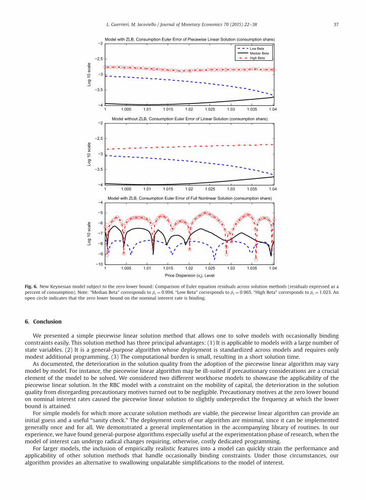
Given that the uncertainty and price dispersion effects may offset or reinforce each other, it is especially important toassess the performance of the piecewise linear method for different calibrations, as well as across a wide range of values fordispersion and for different values of the shock process βt. Fig. 6 shows Euler equation errors for the baseline calibration,expressed as a share of consumption as for the previous model considered. The figure shows errors for three shock sizes:“Median Beta” corresponding to βt ¼ 0:994; “Low Beta” corresponding to βt ¼ 0:965; “High Beta” corresponding toβt ¼ 1:023.15 We find it remarkable that, at worst, the Euler errors stay close to $1 per $1000 of consumption for extremevalues of dispersion even when the zero lower bound binds. As shown in the middle panel of the figure, this magnitude issimilar to the misses for first-order perturbation solution of a model that disregards the zero lower bound. The bottom panelconfirms that the Euler errors are of an economically negligible magnitude for the fully nonlinear solution.

Additional robustness checks can be found in Table B of the online appendix, where we compare key moments fordifferent calibrations of the model that focus on varying the monetary policy rule and steady-state inflation. We find thatthe piecewise linear model continues to perform adequately: if anything, across experiments, it tends to alwaysunderestimate the frequency of ZLB episodes and the volatility of output.

We conclude our discussion of the New Keynesian model with a word of caution: while the range of parameter values forwhich we can solve and find a unique solution for the piecewise linear model is extensive, our numerical routines for thefully nonlinear solution encountered convergence problems for very persistent shocks, for low values of the price rigidity,and for monetary policy rules with a small inflation response. We conjecture – as many others have already done – that theNew Keynesian model might be afflicted by several pathologies near the zero lower bound that can make the identificationof global solutions especially challenging. These issues have been analyzed and discussed by, among others, Benhabib et al.(2001), Braun and Waki (2010), and Aruoba and Schorfheide (2013). These pathologies seem to afflict the New Keynesianmodel in particular and are not a general feature of all models with occasionally binding constraints.

13 For the linear and piecewise linear solutions considered, we linearize around a non-zero inflation rate. Perturbation solutions around a zero inflationpoint would imply that price dispersion is constant. In that special case, dispersion entirely drops out of the linearized set of conditions for an equilibrium.See Schmitt-Grohe and Uribe (2007) for a discussion of dispersion in a New Keynesian model. See also Figures A and B in Section B of the online appendix.

14 In a general equilibrium setting, the response of dispersion is also influenced by precautionary motives. We confirmed that the piecewise linearsolution understates the decrease in dispersion in response to the increase in the discount factor shown in Fig. 5 by checking a nonlinear solution underperfect foresight.

15 For this model, there are three intertemporal errors associated with Eqs. (22)–(24), respectively. The errors for (23) and (24) have magnitude andpatterns similar to those of the Euler equation errors, as is shown in Section B of the online appendix.

1 1.005 1.01 1.015 1.02 1.025 1.03 1.035 1.04−4

−3.5

−3

−2.5

−2Model with ZLB, Consumption Euler Error of Piecewise Linear Solution (consumption share)

Log

10 s

cale

1 1.005 1.01 1.015 1.02 1.025 1.03 1.035 1.04−4

−3.5

−3

−2.5

−2Model without ZLB, Consumption Euler Error of Linear Solution (consumption share)

Log

10 s

cale

Low BetaMedian BetaHigh Beta

1 1.005 1.01 1.015 1.02 1.025 1.03 1.035 1.04−10

−9

−8

−7

−6

−5

−4Model with ZLB, Consumption Euler Error of Full Nonlinear Solution (consumption share)

Log

10 s

cale

Price Dispersion (vt), Level

Fig. 6. New Keynesian model subject to the zero lower bound: Comparison of Euler equation residuals across solution methods (residuals expressed as apercent of consumption). Note: “Median Beta” corresponds to βt ¼ 0:994. “Low Beta” corresponds to βt ¼ 0:965. “High Beta” corresponds to βt ¼ 1:023. Anopen circle indicates that the zero lower bound on the nominal interest rate is binding.


6. Conclusion

We presented a simple piecewise linear solution method that allows one to solve models with occasionally bindingconstraints easily. This solution method has three principal advantages: (1) It is applicable to models with a large number ofstate variables. (2) It is a general-purpose algorithm whose deployment is standardized across models and requires onlymodest additional programming. (3) The computational burden is small, resulting in a short solution time.

As documented, the deterioration in the solution quality from the adoption of the piecewise linear algorithm may varymodel by model. For instance, the piecewise linear algorithm may be ill-suited if precautionary considerations are a crucialelement of the model to be solved. We considered two different workhorse models to showcase the applicability of thepiecewise linear solution. In the RBC model with a constraint on the mobility of capital, the deterioration in the solutionquality from disregarding precautionary motives turned out to be negligible. Precautionary motives at the zero lower boundon nominal interest rates caused the piecewise linear solution to slightly underpredict the frequency at which the lowerbound is attained.

For simple models for which more accurate solution methods are viable, the piecewise linear algorithm can provide aninitial guess and a useful “sanity check.” The deployment costs of our algorithm are minimal, since it can be implementedgenerally once and for all. We demonstrated a general implementation in the accompanying library of routines. In ourexperience, we have found general-purpose algorithms especially useful at the experimentation phase of research, when themodel of interest can undergo radical changes requiring, otherwise, costly dedicated programming.

For larger models, the inclusion of empirically realistic features into a model can quickly strain the performance andapplicability of other solution methods that handle occasionally binding constraints. Under those circumstances, ouralgorithm provides an alternative to swallowing unpalatable simplifications to the model of interest.


Acknowledgments

We are grateful to Urban Jermann and a referee for suggestions that have greatly improved the paper. We are alsoindebted to Chris Gust for many helpful discussions. The views expressed in this paper are solely the responsibility of theauthors and should not be interpreted as reflecting the views of the Board of Governors of the Federal Reserve System or ofany other person associated with the Federal Reserve System. The library of routines that accompanies this paper as well asadditional documentation are available at the following website: http://www2.bc.edu/matteo-iacoviello/research.htm.

Appendix A. Supplementary data

Supplementary data associated with this article can be found in the online version at http://dx.doi.org/10.1016/j.jmoneco.2014.08.005.

References

Adjemian, S., Bastani, H., Karamé, F., Juillard, M., Maih, J., Mihoubi, F., Perendia, G., Ratto, M., Villemot, S., 2011. Dynare: reference manual version 4. DynareWorking Papers 1, CEPREMAP.

Adjemian, S., Juillard, M., 2011. Accuracy of the extended path simulation method in a new Keynesian model with zero lower bound on the nominal interestrate. Unpublished manuscript.

Aruoba, S.B., Fernandez-Villaverde, J., Rubio-Ramirez, J.F., 2006. Comparing solution methods for dynamic equilibrium economies. J. Econ. Dyn. Control 30(12), 2477–2508.

Aruoba, S.B., Schorfheide, F., 2013, Macroeconomic dynamics near the zlb: a tale of two equilibria. NBER Working Papers 19248, National Bureau ofEconomic Research, Inc., July.

Benhabib, J., Schmitt-Grohe, S., Uribe, M., 2001. The perils of Taylor rules. J. Econ. Theory 96 (1–2), 40–69.Blanchard, J.O., Fischer, S., 1989. Lectures on Macroeconomics. MIT Press, Boston, Massachusetts.Blanchard, O., Kahn, C., 1980. The solution of linear difference models under rational expectations. Econometrica 48 (5), 1305.Bodenstein, M., Guerrieri, L., Erceg, C., 2009. The effects of foreign shocks when interest rates are at zero. International Finance Discussion Paper series 983,

Federal Reserve Board.Bodenstein, M., Guerrieri, L., Gust, C., 2013. Oil shocks and the zero bound on nominal interest rates. J. Int. Money Financ. 32, 941–967.Braun, A., Waki, Y., 2010. On the size of the fiscal multiplier when the nominal interest rate is zero. Mimeo, Federal Reserve Bank of Atlanta.Chen, H., Cúrdia, V., Ferrero, A., 2012. The macroeconomic effects of large-scale asset purchase programmes. Econ. J. 122 (564), F289–F315.Christiano, L., Eichenbaum, M., Rebelo, S., 2011. When is the government spending multiplier large? J. Polit. Econ. 119 (1), 78–121.Christiano, L.J., Fisher, J.D.M., 2000. Algorithms for solving dynamic models with occasionally binding constraints. J. Econ. Dyn. Control 24 (8), 1179–1232.den Haan, W.J., Judd, K.L., Juillard, M., 2011. Computational suite of models with heterogenous agents ii: multi-country real business cycle models. J. Econ.

Dyn. Control 35, 175–177.Eggertsson, G.B., Woodford, M., 2003. The zero bound on interest rates and optimal monetary policy. Brook. Pap. Econ. Activity 34 (1), 139–235.Fair, R.C., Taylor, J.B., 1983. Solution and maximum likelihood estimation of dynamic nonlinear rational expectations models. Econometrica 51 (4),

1169–1185.Fernández-Villaverde, J., Gordon, G., Guerrón-Quintana, P.A., Rubio-Ramírez, J., (2012). Nonlinear adventures at the zero lower bound. NBERWorking Papers

18058, National Bureau of Economic Research, Inc. May.Galí, J., 2008. Monetary Policy, Inflation, and the Business Cycle: An Introduction to the New Keynesian Framework. Princeton University Press, Princeton,

NJ.Holden, T., Paetz, M., 2012. Efficient simulation of dsge models with inequality constraints. Working paper, University of Surrey.Judd, K.L., 1992. Projection methods for solving aggregate growth models. J. Econ. Theory 58, 410–452.Judd, K.L., Maliar, L., Maliar, S., 2012. Merging Simulation and Projection Approaches to Solve High-dimensional Problems. Technical Report. NBER working

paper No. 18501.Jung, T., Teranishi, Y., Watanabe, T., 2005. Optimal monetary policy at the zero-interest-rate bound. J. Money Credit Bank. 37 (5), 813–835.Kim, S.H., Kollmann, R., Kim, J., 2010. Solving the incomplete market model with aggregate uncertainty using a perturbation method. J. Econ. Dyn. Control

34 (1), 50–58.Laséen, S., Svensson, L.E.O., 2009. Anticipated Alternative Instrument-rate Paths in Policy Simulations. Technical Report. National Bureau of Economic

Research, Inc. NBER working paper No. 14902.Ljungqvist, L., Sargent, T.J., 2004. Recursive Macroeconomic Theory, 2nd ed. MIT Press, Cambridge, MA.McGrattan, E.R., 1996. Solving the stochastic growth model with a finite element method. J. Econ. Dyn. Control 20 (1–3), 19–42.Nakata, T., 2013. Uncertainty at the zero lower bound. Finance and Economics Discussion Papers 2013–09, Board of Governors of the Federal Reserve

System (U.S.).Preston, B., Roca, M., 2007. Incomplete Markets, Heterogeneity and Macroeconomic Dynamics. Technical Report.Santos, M.S., Peralta-Alva, A., 2005. Accuracy of simulations for stochastic dynamic models. Econometrica 73 (November (6)), 1939–1976.Schmitt-Grohe, S., Uribe, M., 2007. Optimal inflation stabilization in a medium-scale macroeconomic model. In: Schmidt-Hebbel, K., Mishkin, R. (Eds.),

Monetary Policy Under Inflation Targeting, Santiago, Chile, pp. 125–186.Smets, F., Wouters, R., 2007. Shocks and frictions in us business cycles: a Bayesian DSGE approach. Am. Econ. Rev. 97 (3), 586–606.Taylor, J.B., Uhlig, H., 1990. Solving nonlinear stochastic growth models: a comparison of alternative solution methods. J. Bus. Econ. Stat. 8 (1), 1–17.Uhlig, H., 1995. A toolkit for analyzing nonlinear dynamic stochastic models easily. In: Computational Methods for the Study of Dynamic Economies. Oxford

University Press, Oxford, New York, pp. 30–61.Yun, T., 2005. Optimal monetary policy with relative price distortions. Am. Econ. Rev. 95 (1), 89–109.

http://www2.bc.edu/matteo-iacoviello/research.htm



http://refhub.elsevier.com/S0304-3932(14)00123-8/sbref3




























journal of monetary economics - matteo iacoviello

Documents