jürgen bosse* lorentz atom revisited by solving the

Z. Naturforsch. 2017; aop

Jürgen Bosse*

Lorentz Atom Revisited by Solving the Abraham–Lorentz Equation of MotionDOI 10.1515/zna-2017-0182Received March 8, 2017; accepted June 3, 2017

Abstract: By solving the non-relativistic Abraham–Lorentz (AL) equation, I demonstrate that the AL equation of motion is not suited for treating the Lorentz atom, because a steady-state solution does not exist. The AL equation serves as a tool, however, for deducing the appropriate parameters Ω and Γ to be used with the equation of forced oscillations in modelling the Lorentz atom. The electric polarisability, which many authors “derived” from the AL equation in recent years, is shown to violate Kramers–Kronig relations rendering obsolete the extracted photon-absorption rate, for example. Fortunately, errors turn out to be small quantitatively, as long as the light frequency ω is neither too close to nor too far from the resonance fre-quency Ω. The polarisability and absorption cross section are derived for the Lorentz atom by purely classical reason-ing and are shown to agree with the quantum mechanical calculations of the same quantities. In particular, oscilla-tor parameters Ω and Γ deduced by treating the atom as a quantum oscillator are found to be equivalent to those derived from the classical AL equation. The instructive comparison provides a deep insight into understanding the great success of Lorentz’s model that was suggested long before the advent of quantum theory.

Keywords: Atomic Polarisability; Classical Abraham– Lorentz Equation; Radiation Damping.

PACS numbers: 02.30Hq; 03.50.De; 31.15xp; 37.10.-x.

1 IntroductionIn recent years, the classical Lorentz oscillator model serving as an intuitive description of an atom under the influence of the AC electric field associated with a standing wave of visible light has celebrated a revival in quantum optics literature [1, 2]. While the simple one-dimensional classical oscillator model described by an equation of forced oscillations [cf. (4)] with a friction force

proportional to the first time derivative of elongation has many applications besides the Lorentz atom model (e.g. the AC current circuit with impedance and capacity [3] or simplified models of density fluctuations in liquids [4]), the latter has played a special role reflected by its historical development. Attempting to determine the fric-tion force from the conservation of energy using Larmor’s formula, Lorentz arrived at the “radiative reaction force” for small velocities | ( ) |,x t

πε

= 2

30

( ) ( ),6RRef t x tc

(1)

which was generalised by Abraham for arbitrary velocities in 1904. Using (1) as a substitute for the friction force in the classical oscillator model (4) will result in a modified equation of motion, referred to as the Abraham–Lorentz (AL) equation (see, e.g. [2, (2A.43)], [5, ch. 11], [6, ch. 16.2], or [7, ch. 17.2]).

As has been pointed out by Dirac [8], a friction term proportional to the third time derivative of the oscillator elongation has unpleasant implications such as runaway’s even for vanishing external forces and pre-acceleration solutions, which are certainly unphysical. The radiative reaction force, in particular, and the broader problem of finding an adequate equation of motion for a charged par-ticle coupled to its electromagnetic field, in general, have been discussed extensively for more than 100 years. A comprehensive account of these efforts, giving not only an extensive historical overview but also presenting detailed and self-contained derivations of the adequate equations governing the dynamics of charged particles, can be found in the monograph by Spohn [9]. The important message from this thorough mathematical investigation of both the semi-relativistic coupled Maxwell–Newton equations [9, ch. 8] and the fully relativistic Lorentz–Dirac equation [10] is that there is no third time derivative of the particle posi-tion in the appropriate effective equation of motion of a charged particle. This conclusion relies on the smallness of radiation–reaction effects that calls for applying the “sin-gular perturbation theory” to determine the exact effective equation that governs motion on the “critical manifold”.

In the non-relativistic limit, the effective equation of motion of an electron subjected to the force Fex takes the simple form [9, 11]

*Corresponding author: Jürgen Bosse, Fachbereich Physik, Freie Universität Berlin, 14195 Berlin, Germany, E-mail: [email protected]. http://orcid.org/0000-0002-7600-509X

Bereitgestellt von | Freie Universität BerlinAngemeldet | [email protected] Autorenexemplar

Heruntergeladen am | 16.07.17 09:39

mailto:[email protected]

http://orcid.org/0000-0002-7600-509X

2 J. Bosse: Solving the Abraham–Lorentz Equation of Motion

τ τ

π= + =

2

ex ex 30

, ,6

emmc

r F Fε

(2)

which for the one-dimensional Lorentz atom model with a linear restoring force and an additional explicitly time-dependent force, ω= − +2

ex 0 ( ),F m x f t reduces to

τω τω

++ + =

2 20 0

( ) ( ) .f t f tx x xm

(3)

It must be mentioned that this result was obtained earlier as an approximation to the Lorentz–Dirac equa-tion [12] as well as to a non-relativistic equation based on a generalised quantum Langevin approach [13].

In view of the result (3), the reader may wonder about the motivation for the present investigation. Obviously, a large number of authors (including myself) in the optics and ultra-cold gases community were not aware of the fundamental results [10, 11] – a conclusion drawn from the frequently employed AL equation attended by using an incorrect Lorentz atom polarisability in many high-impact publications in recent years (see, e.g. [1, 2, 5, 14]). The con-fusing situation with an equation as simple as the AL (26) calls for a pedestrian’s view on the problem.

In Section 2, a concise review is presented of the unique solution of the forced-oscillations equation, inclu-sive of its steady-state limit, by introducing classical elon-gation-response and -relaxation functions.

In Section 3, the unique solution of the AL equation for given initial values (x0, v0, b0) is determined. The unique solution is shown to be a “runaway” implying the non-existence of a steady-state solution and spotting the AL equation of motion as an inappropriate tool for describ-ing the Lorentz atom. The forced-oscillation equation is suggested, instead, to do the job together with oscillator parameters (Ω, Γ) derived from the AL equation. In this context, a widely spread error is pointed out regarding the “complex polarisability” of the Lorentz atom (see, e.g. [1, section 2.1], [2, section 2A]).

In Section 4, for a quantum mechanical system perturbed by an oscillatory external field, a represen-tation-free perturbation expansion in the field strength is presented for an expectation value. With its help, the “absorbed power” (dipole moment to first order) and the “AC Stark shift” (energy to second order) are derived in terms of the dipole–dipole response function or rather the complex polarisability. The quantum mechanical response function is evaluated for a charged quantum oscillator and compared to the classical dipole–response function of the Lorentz atom derived in Section 3. Perfect agreement between the classical and quantum

mechanical calculation is found, which renders an explanation for the great success of the classical Lorentz atom.

In Section 5, the reader finds a Summary and Con-clusions. In the Appendix, the unique solution of the AL equation of motion for given initial values (x0. v0, b0) is presented in terms of classical response and relaxation functions. In addition, the Appendix contains a short compendium on integral transforms used in this work.

2 Classical Oscillator

2.1 Response and Relaxation Functions

The ordinary second-order differential equation

Γ Ω+ + = 2( ) ( ) ( ) ( ) /x t x t x t f t m (4)

with positive constants (m, Ω, Γ) and external force f(t) has, for given initial values

= = 0 0 0 0( ), ( ),x x t v x t (5)

a unique solution. Finding this solution belongs to the first exercises in every maths course on ordinary differ-ential equations. For physical applications of the forced oscillations (4), it is useful to cast the unique solution into the intuitive form (t ≥ t0),

0

0 0 0 0 0( , ) ( ) i ( )

d i ( ) ( ),t

t

x t t t t x t t mv

t t t f t

φ χ

χ

= − + −

+ −′ ′ ′∫

(6)

with abbreviations

ζ ζζ ζ ζ ζχ φ

ζ ζ ζ ζ

−−= = ≥− −

2 11 21 2

1 2 1 2

e ee( ) , ( ) ( 0)i ( )

t tt tet t tm

(7)

denoting, respectively, classical elongation-response and (normalised)-relaxation functions defined, at this stage, for non-negative arguments only. Here ζ1 and ζ2 denote roots of the characteristic polynomial associated with (4), ζ Γ Γ Ω= − ± −2 2

1,2 / 2 ( / 2) , which obey

ζ ζ ζ Ω ζ ζ Γℜ < = + = −21,2 1 2 1 2[ ] 0, , . (8)

Due to negative real parts of both roots ζ1 and ζ2, the functions φ(t) and χ(t) will decay to zero if time arguments grow large.

It is convenient to extend the definitions of response and relaxation functions to negative time arguments. In



J. Bosse: Solving the Abraham–Lorentz Equation of Motion 3

accordance with quantum mechanical linear-response theory (see Section 4 below), I postulate

χ χ χ φ φ φ∗ ∗− = − = − = =( ) ( ) ( ) , ( ) ( ) ( ) .t t t t t t (9)

After introducing phase angle ϑ and frequency Ω by

Ω Γ Ω ΓΓϑ Ω

Ω Γ Ω Ω Γ

− = = − ≤

2 2

2 2

( / 2) , > / 2arctan , ,

2 i ( / 2) , / 2

(10)

which will be real-valued, if Γ < 2Ω (low-damping regime), the response and relaxation functions may be expressed in the more descriptive way,

| | | |2 2sin( ) cos( | | )( ) e , ( ) e .

cosit tt tt t

m

Γ ΓΩ Ω ϑχ φ

ϑΩ

− − −= =

(11)

Here occurrence of |t| reflects the symmetry intro-duced in (9).

2.2 Steady-State Elongation

The initial time t0 in (5) and (6) is properly interpreted as the instant when the external force f(t) is switched on. After switch on, the elongation x(t, t0) will at first depend on t0 and the initial values (x0, v0) until “transients” have died off due to relaxation processes, and the system described by (4) acquires a steady state. The corresponding steady-state elongation ξ(t) is found by switching on the force f(t) adiabatically and choosing t0 = −∞ in (6),

ξ χ

∞ ′−

→−∞′ ′ ′= = −∫

00 0

( ) lim ( , ) d e i ( ) ( ).ot

tt x t t t t f t t

(12)

The adiabatical switch on is described by replacing under the integral in (6): f(t′)→f(t′)e−o(t−t′) (o > 0). Subse-quent substitution t − t′→t′ results in (12). It is understood from hereon that o→0 is taken after time integrations have been performed – without repeatedly employing the explicit notation limo→0. This convention regarding treatment of the small positive frequency o will be used throughout.

It is to be noted that the steady-state elongation (12) is independent of initial values (x0, v0), because the general solution of the homogeneous equation (4) for f(t) ≡ 0, xh

(t, t0) = φ(t − t0)x0 + iχ(t − t0)mv0, which does depend on initial conditions, will vanish in the steady-state limit. This independence of initial values is a physical require-ment on a steady-state solution, because initial values x0 and v0 are not (and cannot usually be) measured.

2.3 Dynamical Susceptibility

If the force entering the integrand in (12) is represented by its Fourier integral, the steady-state solution will also appear in the Fourier expanded form

ω ω ω

ξ ω ξ ω ξ χ ωπ

∞

−∞= − = +∫ 1( ) d exp( i ), ( i ) ,

2t t o f

(13)

with the dynamical susceptibility ω ω

χ ω ξ+ = ( i ) /o f deter-mining the ratio between Fourier-transformed elongation and force. Here χ ( ),z the Fourier–Laplace transform (FLT, see Appendix for details) of the response function χ(t), has been introduced. For the classical response and relaxa-tion functions given in (11), FLTs are readily calculated (s = signℑ[z]),

Γχ φ

Ω Γ Ω Γ

+= =− + − +

2 2

1 / i( ) , ( ) .( i ) ( i )m z sz z

z z s z z s (14)

For the dynamical susceptibility, one has

Ωχ ω χ χ ω χ ω

Ω ω ωΓ′+ = ≡ + ″

− −

2

02 2( i ) ( ) i ( )i

o

(15)

with real and imaginary parts

Ω ω Ωχ ω χ

Ω ω ωΓ

−′ =− +

2 2 2

02 2 2 2( )( ) ,

( ) ( ) (16)

ωΓΩχ ω χ

Ω ω ωΓ″ =

− +

2

02 2 2 2( ) ,( ) ( )

(17)

and the static susceptibility

χ χ χ

Ω′= = =

0 21 (i ) (0).o

m (18)

It is worth pointing out the close relationship between response and relaxation functions known as Kubo identity,

2 2

( ) 1 i ( )( ) ( ) ,z z tz tm m

φ φχ χ

Ω Ω

+≡ ⇔ ≡

(19)

which is reflected by (11) and (14), and also mentioning the exact rewriting

Γ ΓΩχΩ

χΓΩ Γ Γ

Ω Ω

= + − + + +

02 2( ) ,

i i2 2

zz s z s

(20)

which highlights the resonance patterns emerging near ω Ω= ± (cf. (10)) in case of Γ/Ω 1.




Finally, it is important to notice that the two ingredi-ents χ′(ω) = χ′(−ω) and χ″(ω) = −χ″(−ω) of the dynamical susceptibility are intimately connected via Kramers–Kro-nig relations, cf. (a6) below. These dispersion relations are an immediate consequence of the generalised susceptibil-ity χ ( )z appearing as the Fourier–Laplace transform of the response function χ(t). Violation of Kramers–Kronig relations is an indicator for a faulty determination of χ ω + ( i ).o Similarly, experimental results on χ′(ω) and χ″(ω) would not be trustworthy, if available measured data permitted someone to demonstrate violation of Kramers–Kronig relations.

2.4 Oscillatory Force

The steady-state solution (12) acquires a specially simple form, if one assumes a sinusoidal t dependence of fre-quency ω for the force,

ωω −= ≡ ℜ i0 0( ) cos( ) [e ],tf t f t f (21)

with real f0 and ω. Inserting this force into (12) results in the steady-state elongation

ωξ χ ω

χ ω ω χ ω ω

−= ℜ +′= + ″ i

0

0

( ) [ ( i ) e ][ ( )cos( ) ( )sin( )]

tt o ft t f

(22)

that may be cast into the clearly arranged form

ξ ω ϕ= −( ) cos( )t A t (23)

with ω-dependent amplitude and phase shift

Ω χ Ω χ

ΩΓΩ ω ωΓωΓ Ω ω

ϕ πΩ ω

= ≤ =− + − −= + −

2 20 0 0 0

m2 2 2 2

2 2

2 2

,( ) ( )

1 sign( )arctan .2

f fA A

(24)

The oscillator picks up energy from the oscillatory force and dissipates this energy via friction (Γ > 0). The work done by the external force during time interval (t, t + dt) amounts to ξ ξ ξ+ − = [ ( d ) ( )] ( ) d ( ) ( ).t t t f t t t f t Inte-grating this energy over an oscillation period T = 2π/ω and dividing by T results in the average absorbed power

ω ξ ωχ ω= = ″ ≥∫ 2

00

1 1( ) d ( ) ( ) ( ) 0.2

TP t t f t f

T (25)

A glance at (17) shows that no power will be absorbed, if a constant external force is applied (ω = 0), while maximum power absorption will be achieved, if the “resonance value” ωr = ± Ω is chosen for the applied

oscillatory-force frequency ω. Finally, it is to be noted that the driven elongation ξ(t) develops its amplitude maximum Am for a different driving-field frequency

ω Ω Γ Ω= ± − 2 2m 1 /(2 ). Moreover, both ωr and ωm differ

from Ω in (11). For ΓΩ, however, the three frequencies ω Ω ω< <m r| | | | will differ only slightly and merge for Γ→0.

3 Lorentz Atom

3.1 AL Equation

The forced oscillations (4) presents an ingenious model first suggested by Lorentz for describing an atom under the influence of visible light. Lorentz assumed an electron (charge q = −e, mass m = me) that is bound to the atomic nucleus by a restoring force fΩ(t) = − mΩ2x(t) and subject to a friction force

ΓΓ= − ( ) ( ).f t m x t If light is shining on

the atom, this electron will, in addition, be exposed to an oscillating force f(t) = qE0 cos(ωt) exerted on a charge by the electric field associated with a standing light wave of frequency ω (neglecting much smaller magnetic field contributions). While the value of the restoring force parameter Ω2 was roughly known, because Ω ≈ 1015 s−1 could be detected by finding the light-wave frequency ωr “in resonance” with the atom, there was little experi-mental information on the extremely small but finite damping constant (ΓΩ) at the end of the 19th century. In summary, the Lorentz model parameters Ω and Γ had to be determined from theoretical reasoning.

In the AL equation of motion (see, e.g. [6, (16.9)],

τ ω− + = 20( ) ( ) ( ) ( ) / ,x t x t x t f t m (26)

the radiation–reaction force τ= RR ( ) ( )f t m x t (1)

replaces the unknown friction force Γ

Γ= − ( ) ( )f t m x t of the forced-oscillation equation of motion (4), while the resonance frequency that determines the restor-ing force has been denoted by ω0 here, for clarity reasons. The radiation–reaction force accounts for the energy loss that the accelerated electron will suffer due to Hertz radiation of electromagnetic waves. Here τ = 2rcl/(3c) (cf. (2)) denotes the time it “takes light to pass by an electron” with classical charge radius rcl = e2/(4πε0mc2), permittivity ε0, and light velocity c in vacuum. One finds τ ≈ 10−23 s resulting in the small parameter τω0 ≈ 10−8 for an atomic electron.

In view of the smallness of the characteristic time τ and the dimensionless parameter (τω0), it is tempting to rewrite the AL equation




20

120

2 20

2 2 20 0

dd

d1dd1 ( )d

( ) ( ) ( ).

fx x xm t

fxt m

fxt m

f t f tx xm

ω τ

τ ω

τ τ ω

τω τω τ

−

= − + +

= − − +

= + + − +

+= − − + +

O

O

(27)

In the representation (27), one of the AL equation’s strange properties shows up: the acceleration at (present time) t, ( ),x t is induced by a force τ τ+ ≈ + ( ) ( ) ( )f t f t f t to be applied at (future time) t + τ. Leaving aside philosophi-cal questions arising from the “pre-acceleration” problem (see, e.g. [7, section 17.7], [5, section 11.2.2]), the expansion (27) shows that the widely used AL equation could be approximated by the effective equation of motion cited in (3), which is obtained by replacing

Γ τω Ω ω τ→ → → + 2 2 20 0, , ( ) ( ) ( )f t f t f t (28)

in the equation of forced oscillations (4). The same argument used in (27) for approximating the AL equa-tion was applied on the relativistic Lorentz–Dirac equa-tion in [12].

At this stage, instead of further endeavours to find a substitute for (26) by exploiting the smallness of τω0, let us solve the AL equation of motion itself.

3.2 Roots of AL Characteristic Polynomial

The inhomogeneous third-order ordinary differential equation with constant coefficients may be solved by “brute force”. It is straightforward to find the unique solu-tion of (26) for given initial conditions

= 0 0 0 0 0 0( ), = ( ), = ( ).x x t v x t b x t (29)

The unique solution = +h pAL 0 AL 0 AL 0( , ) ( , ) ( , ),x t t x t t x t t

which is the sum of the general solution of the homoge-neous and one particular solution of the inhomogene-ous equation, will then be used to derive the steady-state elongation ξAL(t) = xAL(t, t0→ −∞) following the procedure applied in Section 2.2.

Denoting by ζ1, ζ2, ζ3 the roots of the characteristic polynomial associated with (26)

ζ τζ ω− + =2 3 20 0, (30)

one finds, as expected for the roots of a third-order poly-nomial, a pair of complex conjugate besides a real root

ζ ζ ζ

τ= + = − = −1 2 3

1i , 2 , i ,u v u u v

(31)

with real and imaginary parts of ζ1 given by

τ τ

τω τω τ ω

− −= − ≤ = ≥

= + − +

2 2

13

2 20 0 0

( 1) 10, 0,6 2 3

31 (9 12 81 ) ,2

w wu vw w

w

(32)

where 0 ≤ w ≤ 1. Two identities,

τ τ ω τ− + ≡ + ≡ −2 2 2 2 202 3 , 3 (3 8 )u u v u v u (33)

valid for all values of ω0τ ≥ 0, are mentioned here for later use.

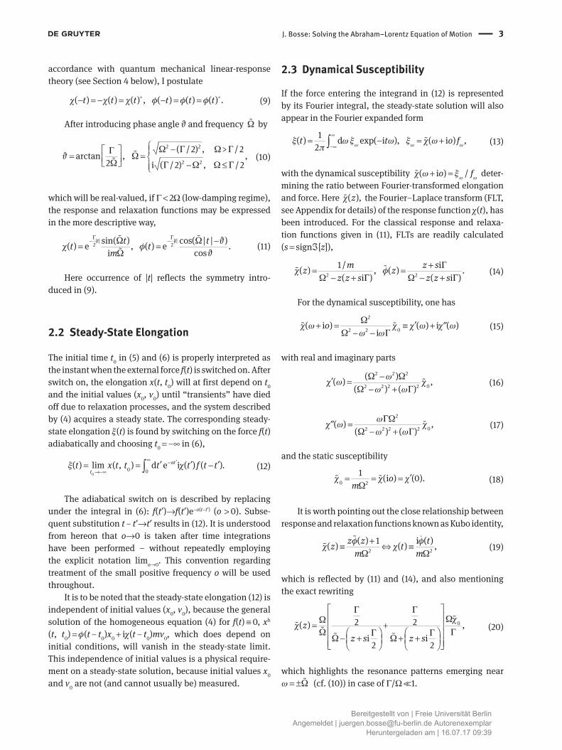
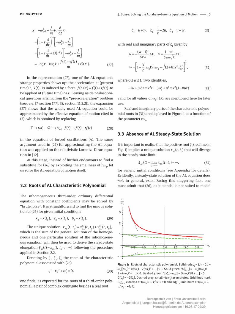
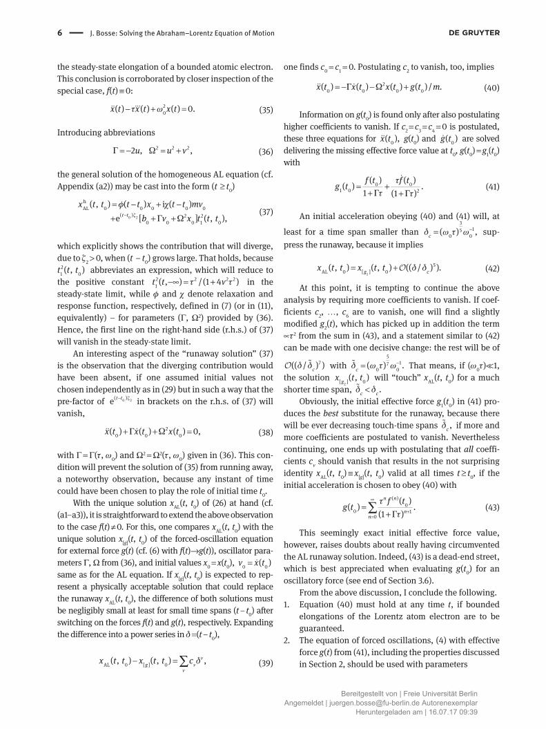
Real and imaginary parts of the characteristic polyno-mial roots in (31) are displayed in Figure 1 as a function of the parameter τω0.

3.3 Absence of AL Steady-State Solution

It is important to realise that the positive root ζ2 (red line in Fig. 1) implies a unique solution xAL(t, t0) that will diverge in the steady-state limit,

0

AL AL 0( ) lim ( , ) ,t

t x t tξ→−∞

= = ∞ (34)

for generic initial conditions (see Appendix for details). Evidently, a steady-state solution of the AL equation does not, in general, exist. Facing this staggering fact, one must admit that (26), as it stands, is not suited to model

0.5

–1

1

2

3

zω0

τ ω01.0 1.5 2.0 2.5 3.0 3.5

Figure 1: Roots of characteristic polynomial. Solid red: ζ2 = 1/τ − 2u = ω0[(τω0)−1 +(τω0) − 2(τω0)3 + …] > 0. Solid green: ℜ[ζ1, 3] = − ω0[(τω0)/ 2 − (τω0)3 + …] < 0. Dashed green: ℑ[ζ1] = ω0[1 − 5(τω0)2/8 + …] > 0, ℑ[ζ3] = −ℑ[ζ1]. Dashed grey: small −(τω0) asymptotes. Grid lines mark ℑ[ζ1,3] extrema at (τω0 = 0, v/ω0 = ±1) and ℜ[ζ1,3] minimum at (τω0 = 2, u/ω0 = −1/4).




the steady-state elongation of a bounded atomic electron. This conclusion is corroborated by closer inspection of the special case, f(t) ≡ 0:

τ ω− + = 20( ) ( ) ( ) 0.x t x t x t (35)

Introducing abbreviations

Γ Ω= − = +2 2 22 , ,u u v (36)

the general solution of the homogeneous AL equation (cf. Appendix (a2)) may be cast into the form (t ≥ t0)

ζ

φ χ

Γ Ω−

= − + −

+ + +0 2

hAL 0 0 0 0 0

( ) 2 20 0 0 1 0

( , ) ( ) i ( )e [ ] ( , ),t t

x t t t t x t t mvb v x t t t

(37)

which explicitly shows the contribution that will diverge, due to ζ2 > 0, when (t − t0) grows large. That holds, because

21 0( , )t t t abbreviates an expression, which will reduce to

the positive constant 2 2 2 21 ( , ) /(1 4 )t t vτ τ−∞ = + in the

steady-state limit, while φ and χ denote relaxation and response function, respectively, defined in (7) (or in (11), equivalently) – for parameters (Γ, Ω2) provided by (36). Hence, the first line on the right-hand side (r.h.s.) of (37) will vanish in the steady-state limit.

An interesting aspect of the “runaway solution” (37) is the observation that the diverging contribution would have been absent, if one assumed initial values not chosen independently as in (29) but in such a way that the pre-factor of ζ− 0 2( )e t t in brackets on the r.h.s. of (37) will vanish,

Γ Ω+ + = 20 0 0( ) ( ) ( ) 0,x t x t x t (38)

with Γ = Γ(τ, ω0) and Ω2 = Ω2(τ, ω0) given in (36). This con-dition will prevent the solution of (35) from running away, a noteworthy observation, because any instant of time could have been chosen to play the role of initial time t0.

With the unique solution xAL(t, t0) of (26) at hand (cf. (a1–a3)), it is straightforward to extend the above observation to the case f(t) ≠ 0. For this, one compares xAL(t, t0) with the unique solution x[g](t, t0) of the forced-oscillation equation for external force g(t) (cf. (6) with f(t)→g(t)), oscillator para-meters Γ, Ω from (36), and initial values x0 = x(t0), = 0 0( )v x t same as for the AL equation. If x[g](t, t0) is expected to rep-resent a physically acceptable solution that could replace the runaway xAL(t, t0), the difference of both solutions must be negligibly small at least for small time spans (t − t0) after switching on the forces f(t) and g(t), respectively. Expanding the difference into a power series in δ =(t − t0),

νν

ν

δ− = ∑AL 0 [ ] 0( , ) ( , ) ,gx t t x t t c

(39)

one finds c0 = c1 = 0. Postulating c2 to vanish, too, implies

Γ Ω= − − + 20 0 0 0( ) ( ) ( ) ( ) / .x t x t x t g t m (40)

Information on g(t0) is found only after also postulating higher coefficients to vanish. If c2 = c3 = c4 = 0 is postulated, these three equations for 0( ),x t g(t0) and 0( )g t are solved delivering the missing effective force value at t0, g(t0) = g1(t0) with

τ

Γτ Γτ= +

+ +

0 0

1 0 2

( ) ( )( ) .

1 (1 )f t f t

g t

(41)

An initial acceleration obeying (40) and (41) will, at

least for a time span smaller than δ ω τ ω−=3

150 0( ) ,c sup-

press the runaway, because it implies

δ δ= +1

5AL 0 [ ] 0( , ) ( , ) (( / ) ).g cx t t x t t O (42)

At this point, it is tempting to continue the above analysis by requiring more coefficients to vanish. If coef-ficients c2, …, c6 are to vanish, one will find a slightly modified g2(t), which has picked up in addition the term ∝τ2 from the sum in (43), and a statement similar to (42) can be made with one decisive change: the rest will be of

δ δ 7(( / ) )cO with δ ω τ ω−=5

170 0( ) .c That means, if (ω0τ)1,

the solution 2[ ] 0( , )gx t t will “touch” xAL(t, t0) for a much

shorter time span, δ δ< .c c

Obviously, the initial effective force g1(t0) in (41) pro-duces the best substitute for the runaway, because there will be ever decreasing touch-time spans δ ,c if more and more coefficients are postulated to vanish. Nevertheless continuing, one ends up with postulating that all coeffi-cients cv should vanish that results in the not surprising identity xAL(t, t0) ≡ x[g](t, t0) valid at all times t ≥ t0, if the initial acceleration is chosen to obey (40) with

τ

Γτ

∞

+=

=+∑

( )0

0 10

( )( ) .

(1 )

n n

nn

f tg t

(43)

This seemingly exact initial effective force value, however, raises doubts about really having circumvented the AL runaway solution. Indeed, (43) is a dead-end street, which is best appreciated when evaluating g(t0) for an oscillatory force (see end of Section 3.6).

From the above discussion, I conclude the following.1. Equation (40) must hold at any time t, if bounded

elongations of the Lorentz atom electron are to be guaranteed.

2. The equation of forced oscillations, (4) with effective force g(t) from (41), including the properties discussed in Section 2, should be used with parameters




Γ ω τ ω τ ω τ

Ω ω ω τ ω τ

= − = − +

= + = − +

2 2 40 0 0

2 2 2 40 0 0

2 [1 2( ) (( ) )]

[1 ( ) / 2 (( ) ]

u

u v

O

O

(44)

for treating the Lorentz atom.My conclusions are corroborated by

– the suggested procedure reproducing the litera-ture result (3) or the equivalent small-τ expan-sion given in (27), if Lorentz atom parameters Γ ω τ→ 2

0 , Ω→ω0 are applied (which neglect terms of order O((τω0)2) compared to 1);

– the parameters (44) exactly reproducing the neat results [15, section (3.2)] obtained for the solution of (35) within a fixed-point analysis for discrete dynamical systems; and

– the parameters (44) implying

Ω Ω Γ

ω τω τω

= − == − +

2 2

2 40 0 0

( / 2)[1 5( ) /8 (( ) )]

vO

(45)

for the resonance frequency in (20). It is shifted from ω0 by the extremely small amount ∆ω τ ω= − 2 3

0 05 /8 due to radiation damping. The same shift has been found in [7, (17.57)] starting from an integrodifferential equation of motion that follows from integrating (35) over time t once and postulating the asymptotic condi-tion τ−

→∞ =/lim [e ( )] 0tt x t to be fulfilled (which

excludes “runaway” solutions).

Finally, let me point out the apparent discrepancy between the resonance frequency shift ∆ω τ ω= − 2 3

0 05 /8 obtained in (45) above and the corresponding shift ∆ω τ ω= − 2 3

0 0 /8 resulting from (3), as it stands. Of course, a shift of order (ω0τ)2 obtained from Ω can only be described correctly by starting with parameters of the same accuracy in (3), i.e. by replacing ω0→ω0[1 −(ω0τ)2/2], Γ ω τ ω τ→ −2 2

0 0[1 2( ) ] in that equation.

3.4 Lorentz Atom Polarisability

Following the conclusion of Section 3.3, item 2, the atomic dipole moment d(t) =( − e)ξ(t), which is induced by the electric field of a standing light wave exerting the force f(t) =( − e)E0 cos(ωt) on the electron (within dipole approx-imation), can be read from (22) after replacing f(t) with the corresponding effective force g(t) from (41)

ω

ω

Γτ ωτχ ω

Γτχ ω

−

−

+ −= ℜ + + ≈ ℜ +

2 i02

2 i0

1 i( ) ( i ) e(1 )

[ ( i ) e ].

t

t

d t o e E

o e E

(46)

Here the small additive term ∝ ωτ was neglected, i.e. the applied force f(t) is assumed to be almost static on a time scale τ, and also Γτ1 was used. The Lorentz atom model allows to account for additional damping processes besides radiative loss by replacing Γ in (46) with a total damping constant Γt

Γ Γ Γ Γ′→ = +t . (47)

In view of the constant dipole moment d(t) = d0 induced by a static field E0,

20 0 0 0d ( ) ( 0)e E Eχ α ω= = = (48)

with α χ= 20e denoting the (static) polarisability, it has

become common to name “complex polarisability” the dynamical dipole susceptibility, α ω χ ω+ = + 2( i ) ( i )o o e [1, section 2.1]. Its real part, the (generalised ω dependent) polarisability

α ω α ω χ ω′= ℜ + = 2( ) [ ( i )] ( ) ,o e (49)

determines a force = −∇

dipUF acting on the atom in the light field, where

α ω χ ω′= − = −

22 2 0

dip1( ) ( )| ( , ) | ( )2 4

EU t er E r

(50)

denotes the “optical dipole potential” that will be iden-tified as the average atomic energy shift, known as “AC Stark effect” in Section 4.5 below. Within classical elec-trodynamics, the optical dipole potential can only be made plausible to within a factor of 2, because one has

ω χ ω′− ⋅ = − 2 20 0( ) cos( ) ( ) / 2t t e Ed E for the time-averaged

potential energy of an electric dipole moment in an exter-nal electric field.

3.5 Absorption and Scattering of Radiation by the Lorentz Atom

The imaginary part of the dynamical dipole susceptibil-ity, α ω χ ω′′ℑ + = 2[ ( i )] ( ) ,o e via (25) determines the average power P(ω) absorbed by the atom from the electric field, which implies the absorption cross section 0 0( / ,c ω= wavelength at resonance, divided by 2π),

ΓΓ ωωσ ω π

ω ω ωΓ=

− +

22 t

abs 02 2 2 2 20 0 0 t

( )( ) = 6/ 2 ( ) ( )

PcEε

(51)

that obeys the famous f-sum rule,

πω σ ω

∞=∫

2

abs00

d ( ) ,2

ec mε

(52)




also known as the “dipole sum rule” in the present context. It must be emphasised that the f-sum rule, valid for both classical and quantum mechanical systems, states the fol-lowing interesting fact. The integrated absorption cross section on the r.h.s. of (52) is determined by the ratio e2/m alone. It does not depend on further details of the system, here represented by oscillator frequency and damping constants.

A photon-absorption rate Γabs(ω) has been considered in [1, section 2.1], which is determined by χ″(ω), too. From quantum-mechanical scattering theory, one finds (Θ(x) denotes unit-step function)

χ ω ωΓ ω Θ ω Θ ω

ω

′′= =

2 2abs 0

( ) ( )( ) ( ) ( ),2

Pe E

(53)

if the atom is assumed in its electronic ground state (i.e. at zero temperature) when hit by photons. In (53), Γabs( − ω) = 0 for ω > 0 expresses the fact that an atom in its ground state cannot loose energy by stimulated (or spon-taneous) emission of a photon of energy ħω. It can only win energy by absorbing a photon of energy ħω.

Finally, the time-dependent dipole moment induced by the oscillatory external field (46) will produce an electromagnetic field that in the far-field dipole approxi-

mation π

−= × ×

rad 2

0

( / ) 1( , ) , 4d t r c

r r cc rr rE B e

ε may be inter-

preted in terms of a radiation-scattering cross Section [2, (2A.48)], [7, (17.63)]

π ωσ ω

Ω ω ωΓ=

− +

42

sc cl 2 2 2 2t

8( )3 ( ) ( )r

(54)

ω ω ω ω

ωΓπ ω ω

ω ω ω Γ

ω ω

→ ≈ − +

4 40 0

2 22 00 02 2

0 0 t

0

/ ,( / 2)

6 ,( ) ( / 2)

1,

from which well-known scattering regimes are easily identified as limiting cases: Rayleigh scattering for ωΩ, Thomson scattering for ωΩ, and, for ω ≈ Ω, the resonant Lorentz scattering exhibiting the characteristic line shape with “full width at half maximum”, Γt, and “peak cross section”

π Ω Γσ Ω π

ΓΓ

= =

222 2

sc cl 02tt

8( ) 6 .3r

(55)

Here rcl = 3cτ/2 denotes the classical electron radius, and oscillator parameters are given by Ω = ω0 and total decay constant Γt = Γ + Γ′ with Γ τω= 2

0.

As opposed to the statement in [7, (17.72)] that refers to all ω, (51) and (54) imply σ ω σ ω σ ω= +L L L

abs s r( ) ( ) ( )c for fre-quencies |ω − ω0 | ω0 only, i.e. for the resonant Lorentz absorption (or total) cross section. The total cross section is composed of a scattering contribution σ ωL

sc( ), spelled out in (54) (ω ≈ ω0), and a “reaction cross section” σ ωL

r ( ) with the same Lorentz resonance denominator but Γ replaced with ΓΓ′ in the numerator. Consequently, σ ωL

abs( ) must be given by σ ωLsc( ) with Γ replaced by ΓΓt

in the numerator, which is easily verified from (51). The reason for the discrepancy with [7] will become clear in Section 3.6.

3.6 Pitfalls

Regarding the classical model of the atomic complex polarisability, much confusion has been created in the literature by erroneous conclusions drawn from the AL equation of motion, (26), with oscillatory external force f(t) = f0 cos(ωt). In [1, 2, 5, 7] for example, and in numerous other publications, authors searched for a particular solu-tion of (26) that oscillates with frequency ω of the driving force. Indeed, there is one such solution

ω ω ω τω ω

ω ω τω

− +=

− +

2 2 3osc 0 0

2 2 2 3 20

( )cos( ) sin( )( ) ,

( ) ( )t t f

x tm

(56)

which can be easily checked by inserting xosc(t) into (26). But xosc(t) is not the steady-state solution of the inhomo-geneous AL equation. As according to (34), such a steady-state solution does not exist. That brought me to rule out the AL equation of motion as a candidate for describing the Lorentz atom elongation.

It must be emphasised that, in contrast to my find-ings, (56) is frequently claimed to present the steady-state solution to the AL equation with oscillatory force, which is not true as I demonstrated in Section 3.3. As xosc(t) is not the steady-state solution, we are not allowed to interpret (56) as if it were the analog of (22). Extracting from (56), a “susceptibility”

ωω

ω ω τω ω= =

− −

20

0 02 2 3 20 0

1( ) , i

X X Xm

(57)

is a frequently repeated mistake that – is found already in the high-impact monograph [7],

where in [7, (17.60 − 61)] a non-radiative decay constant Γ′ was assumed in addition to the radiative decay constant Γ τω= 2

0, both of which were combined into a total decay constant Γt(ω) = Γ′ +(ω/ω0)2Γ, which is




evidently not constant. Moreover, Γt(ω) violates the f-sum rule and suppresses the high-frequency Thom-son scattering in [7, (17.63)]. According to my find-ings in (44–46), the total decay rate must here read Γt = Γ′ + Γ as arrived at in (47) above, which will repair the mentioned deficiencies.

Deficiencies have been repaired in the third edi-tion of the book, see [6, (16.74) and (16.77)].

– was made in the monograph [5, Ex. 11.4, p. 468] implicitly, when claiming Γ = τω2 instead of the cor-rect result (44),

– has been carried on into the optical-dipole potential community by the very informative and often cited review article [1, section 2.1],

– is even found in the more recent monographs [2, 14], where it shows up in [2, (2A.53)] and [14, (7.31)] and again, as a nasty suppressor of Thomson scattering, in [2, (2A.48)].

– would also result if one erroneously applied to (26) the mnemonic trick that is so helpful in remember-ing χ ω + ( i ).o Namely, Fourier transforming (4) that is, of course, obeyed by the steady-state elongation ξ(t),

ω ω

ω

ω ω Γ Ω ξ

χ ω ξ−

− + − + == +

2 2

1

[( i ) ( i ) ][ ( i )] ,

m fo

(58)

and subsequently reading from the transformed equation of motion (58) for the dynamical susceptibil-ity the result (15).

Note that the “short-cut” (58) works out alright only, because I proved in Section 2.2 above that (4) does indeed have a unique steady-state solution. The

same, however, does not hold true for the AL equation (26) as I demonstrated in Section 3.3.

But why can X(ω) not serve as a proper dynamical suscep-tibility, anyway? Answer: Because it does not obey Kram-ers–Kronig relations,

[ ( )][ ( )] d ,XX ωω ω

π ω ω

∞

−∞

ℑℜ ≠−∫−1

(59)

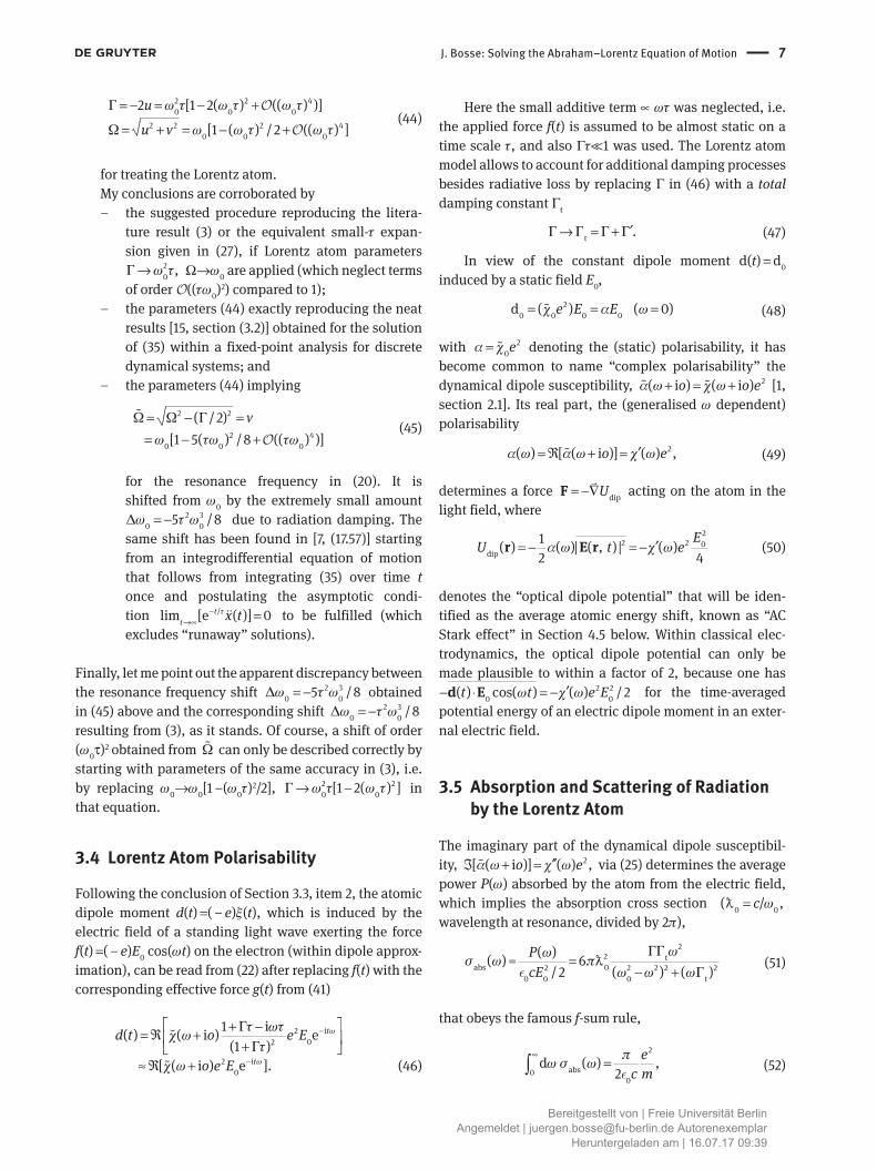
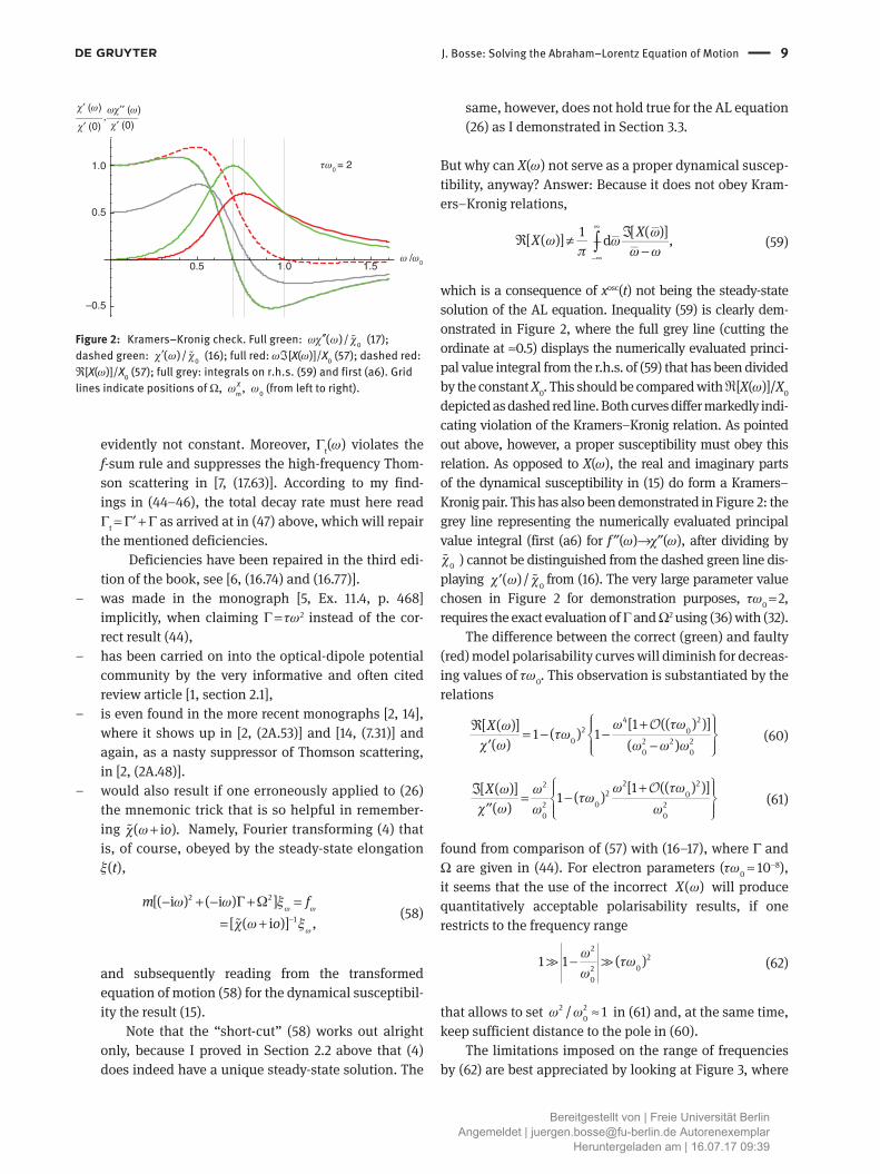
which is a consequence of xosc(t) not being the steady-state solution of the AL equation. Inequality (59) is clearly dem-onstrated in Figure 2, where the full grey line (cutting the ordinate at ≈0.5) displays the numerically evaluated princi-pal value integral from the r.h.s. of (59) that has been divided by the constant X0. This should be compared with ℜ[X(ω)]/X0 depicted as dashed red line. Both curves differ markedly indi-cating violation of the Kramers–Kronig relation. As pointed out above, however, a proper susceptibility must obey this relation. As opposed to X(ω), the real and imaginary parts of the dynamical susceptibility in (15) do form a Kramers–Kronig pair. This has also been demonstrated in Figure 2: the grey line representing the numerically evaluated principal value integral (first (a6) for f ″(ω)→χ″(ω), after dividing by χ 0 ) cannot be distinguished from the dashed green line dis-playing 0( ) /χ ω χ′ from (16). The very large parameter value chosen in Figure 2 for demonstration purposes, τω0 = 2, requires the exact evaluation of Γ and Ω2 using (36) with (32).

The difference between the correct (green) and faulty (red) model polarisability curves will diminish for decreas-ing values of τω0. This observation is substantiated by the relations

4 22 0

0 2 2 20 0

[1 (( ) )][ ( )] 1 ( ) 1( ) ( )X ω τωω

τωχ ω ω ω ω

+ℜ = − − ′ −

O

(60)

2 222 0

02 20 0

[1 (( ) )][ ( )] 1 ( )( )X ω τωω ω

τωχ ω ω ω

+ℑ = − ′′

O

(61)

found from comparison of (57) with (16–17), where Γ and Ω are given in (44). For electron parameters (τω0 ≈ 10−8), it seems that the use of the incorrect ( )X ω will produce quantitatively acceptable polarisability results, if one restricts to the frequency range

ωτω

ω−

22

020

1 1 ( )

(62)

that allows to set ω ω ≈2 20/ 1 in (61) and, at the same time,

keep sufficient distance to the pole in (60).The limitations imposed on the range of frequencies

by (62) are best appreciated by looking at Figure 3, where

ω /ω0

τω0 = 21.0

0.5

–0.5

0.5 1.0 1.5

,χ′ (0)

χ′ (ω) ωχ′′ (ω)

χ′ (0)

Figure 2: Kramers–Kronig check. Full green: 0( )/ωχ ω χ′′ (17); dashed green: 0( )/χ ω χ′ (16); full red: ωℑ[X(ω)]/X0 (57); dashed red: ℜ[X(ω)]/X0 (57); full grey: integrals on r.h.s. (59) and first (a6). Grid lines indicate positions of Ω, m,Xω ω0 (from left to right).




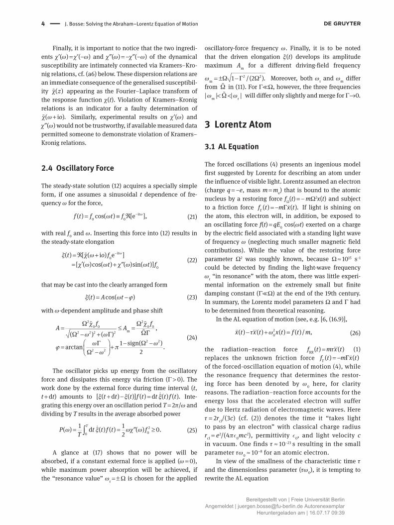
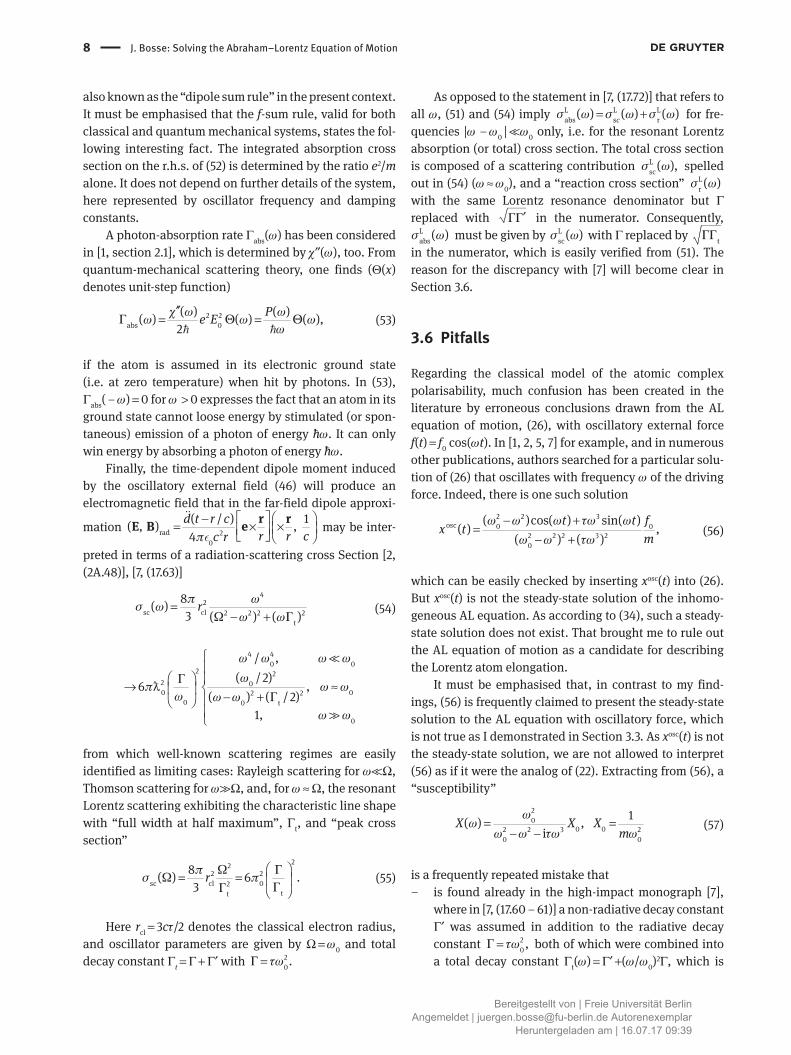
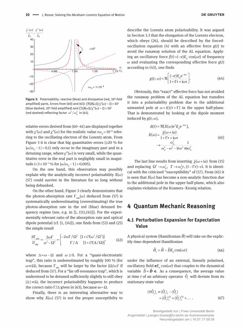
relative errors derived from (60–61) are displayed together with χ′(ω) and χ″(ω) for the realistic value τω0 = 10−8 refer-ring to the oscillating electron of the Lorentz atom. From Figure 3 it is clear that big quantitative errors (±20 % for |ω/ω0 − 1 | ≈ 0.1) only occur in the imaginary part and in a detuning range, where χ″(ω) is very small, while the quan-titative error in the real part is negligibly small in magni-tude (<3 × 10−5 % for |ω/ω0 − 1 | > 0.005).

On the one hand, this observation may possibly explain why the analytically incorrect polarisability X(ω) (57) could survive in the literature for so long without being debunked.

On the other hand, Figure 3 clearly demonstrates that the photon-absorption rate Γabs(ω) deduced from (57) is systematically underestimating (overestimating) the true photon-absorption rate in the red (blue) detuned fre-quency regime (see, e.g. in [1, (11),(41)]). For the experi-mentally relevant ratio of the absorption rate and optical dipole potential (cf. [1, (14)]), one finds from (53) and (25) the simple result

ωΓ Ω ω ΩΓ ωΓΓ ∆ ∆ Ωω Ω

− += = +−

2 2 2abs

2 2dip

2 / [1 ( / )]2 ,/ [1 ( / )]U

O

O

(63)

where Δ = ω − Ω and ω ≥ 0. For a “quasi-electrostatic trap”, this ratio is underestimated by roughly 100 % (for ωΩ), because Γabs will be larger by the factor (Ω/ω)2 if deduced from (57). For a “far off-resonance trap”, which is understood to be detuned sufficiently slightly to still obey |Δ | Ω, the incorrect polarisability happens to produce the correct ratio Γ/Δ given in (63), because ω ≈ Ω.

Finally, there is an interesting alternative way to show why X(ω) (57) is not the proper susceptibilty to

describe the Lorentz atom polarisability. It was argued in Section 3.3 that the elongation of the Lorentz electron, which obeys (26), should be described by the forced-oscillation equation (4) with an effective force g(t) to avoid the runaway solution of the AL equation. Apply-ing an oscillatory force f(t) =(−e)E0 cos(ωt) of frequency ω and evaluating the corresponding effective force g(t) according to (43), one finds

ω

ωΓτ ωτ

− −= ℜ

+ +

it0( ) e

( ; ) .1 ie E

g t

(64)

Obviously, this “exact” effective force has not avoided the runaway problem of the AL equation but transfers it into a polarisability problem due to the additional unwanted pole at ω = i(1/τ + Γ) in the upper half-plane. That is demonstrated by looking at the dipole moment induced by g(t; ω),

2 i0

20

2 2 3 20 0

d( ) [ ( ) e ],( i )( )

1 i1

i

tt X e EoX

m

ωω

χ ωω

Γτ ωτω

ω ω τω ω

−= ℜ+=

+ +

→− −

(65)

The last line results from inserting χ ω + ( i )o from (15) and replacing Ω ω→2 2

0, Γ ω τ→ 20 , (1 − Γτ)→1. It is identi-

cal with the criticised “susceptibility” of (57). From (65) it is seen that X(ω) has become a non-analytic function due to the additional pole in the upper half-plane, which also explains violation of the Kramers–Kronig relation.

4 Quantum Mechanic Reasoning

4.1 Perturbation Expansion for Expectation Value

A physical system (Hamiltonian Ĥ) will take on the explic-itly time-dependent Hamiltonian

ω= − 0ˆ ˆ ˆ cos( )tH H DE t (66)

under the influence of an external, linearly polarised, oscillatory field eE0 cos(ωt) that couples to the dynamical variable ˆ ˆ .D = ⋅eD As a consequence, the average value at time t of an arbitrary operator ˆ

tO will deviate from its stationary-state value

δ⟨ ⟩ ≡ ⟨ ⟩ − ⟨ ⟩= ⟨ ⟩ + ⟨ ⟩ +…(1) (2)

ˆ ˆ ˆˆ ˆ .

t t t t t

t t t t

O O OO O

(67)

0.95 1.00 1.05

×106

1.10 ω0

τω0 = 1×10–8

ω

–30

–20

–10

10

20

30

40

,χ0

χ′ (ω) χ′′ (ω)

χ0

Figure 3: Polarisability: reactive (blue) and dissipative (red, 106-fold amplified) parts. Errors from (60) and (61): ℜ[X(ω)]/χ′(ω) − 1 × 102 (blue dashed, 106-fold amplified) and ℑ[X(ω)]/χ″(ω) − 1 × 102 (red dashed) reflecting factor 2 2

0/ω ω in (61).




Assuming the perturbing field switched on adi-abatically at time t0 = −∞ (which amounts to replacing E0 cos(ωt′)→e−o(t−t′)E0 cos(ωt′) with o > 0 for all t′ ≤ t), the n-th order in E0 contribution to δ⟨ ⟩ˆ

t tO reads explicitly (τ0 = 0)

τ τ

τ

τ τ χ τ τ

ω τ

−

∞ ∞

−

=

⟨ ⟩ = … …

× −

∫ ∫∏

†0 1

( )ˆ ˆ1 1;

01

ˆ i d d ( , , )

e cos[ ( )]

tn

j

n nt t n nO D

no

jj

O

E t

(68)

with the n-th order response function

χ τ τ

τ τ τ

… =

⟨ … − − … − ⟩

ˆ ˆ 1;

†1 2

( , , )1 ˆ ˆ ˆ ˆ[ [[ , ( )], ( )] , ( )] .

nA B

nn A B B B

(69)

Here = − ˆ ˆ ˆ ˆ( ) exp(i / ) exp( i / )B t tH B tH denotes a Heisenberg operator referring to the unperturbed system, and the stationary-state average is defined as

⟨ ⟩ = =ˆ ˆ ˆ ˆ ˆTr , [ , ] 0A AW H W (70)

with statistical operator Ŵ describing the initial station-ary state of the unperturbed system.

It must be emphasised that δ⟨ ⟩ˆt tO in (67–69) describes

the steady-state deviation from the unperturbed expecta-tion value, which is induced by the external field. Inter-estingly enough, the first-order result ⟨ ⟩(1)ˆ

t tO (written out explicitly in (71) for the induced dipole moment) has the same structure found for the steady-state solution in (12) for the classical oscillator elongation.

4.2 Induced Dipole Moment

For the atomic dipole moment induced by a linearly-polar-ised standing light wave of frequency ω, one reads for the first-order result (1)ˆd( ) tt Dδ= ⟨ ⟩ from (68)

ˆ ˆ 0;0i

ˆ ˆ 0;

d( ) i d e ( ) cos[ ( )][ ( i ) e ],

oD D

tD D

t E to E

τ

ω

τ χ τ ω τ

χ ω

∞ −

−

= −

= ℜ +∫

(71)

with the dipole–dipole response function

χ χ= ⟨ ⟩ = − −

ˆ ˆ ˆ ˆ; ;

1 ˆ ˆ( ) [ ( ), ] ( ),D D D Dt D t D t

(72)

where D is identified with the component in field direc-tion of the atomic dipole-moment operator ˆ .D

The corresponding dynamical dipole susceptibility (“complex polarisability”) resulting from Fourier–Laplace transforming χ ˆ ˆ; ( )D D t according to (a4) may very generally be cast into the form [4]

Ωχ χ

Ω=

− −

2

ˆ ˆ ˆ ˆ2 2; ;( ) (i ).( )

DD D D D

D D

z oz zK z

(73)

This formally exact expression is cited here only to point out the following facts.

– The relaxation kernel ωωπ ω

∞

−∞

′′=

−∫ ( )d( ) DD

KK z

z is deter-

mined by an even, non-negative, and bounded spectral function ω′′( ).DK This generally frequency-dependent “total damping constant” ω ω′′ = ℑ +( ) [ ( i )]D DK K o will inevitably be associated with a resonance-frequency renormalisation via ωℜ +[ ( i )].DK o Such a real con-tribution is missing in [7, (17.60)] resulting in the vio-lation of Kramers–Kronig relations and f-sum rule discussed in Section 3.6 above. Moreover, Γt(ω) in [7, (17.61)] is not bounded.

– The relaxation kernel ( )DK z is the FLT of the dipole memory function KD(t) governing the generalised oscillator equation

φ Ω φ φ′ ′ ′+ + − =∫ 2

ˆ ˆ ˆ ˆ ˆ ˆ; ; ;0( ) ( ) d ( ) ( ) 0

t

D DD D D D D Dt t t K t t t

(74)

with initial conditions φ φ= =ˆ ˆ ˆ ˆ; ;(0) 1, (0) 0,D D D D which

is obeyed by the (normalised) dipole relaxation function. Both, (73) and (74), are formally exact and, in view of Kubo’s identity (19), equivalent statements.

To conclude these general remarks, I emphasise that memory effects may be neglected in some applications, rendering

Γδ ω Γ Γ′′≈ ⇒ ≈ ⇒ ≈( ) 2 ( ) ( ) ( ) iD D DK t t K K z s (75)

a reasonable approximation – as is the case for the quantum oscillator in Section 4.3. Under these circum-stances, (74) reduces to a free-oscillations equation of the same type obeyed by the classical relaxation function φ(t) introduced in Section 2. These remarks on very general quantum mechanical (and quantum statistical) results may illuminate the great success of models such as the Lorentz atom, which are based on the classical forced-oscillations equation of motion.

4.3 Quantum Oscillator

Assuming the eigenvalue problem of the unperturbed Hamiltonian solved (Ĥ | n⟩ = | n⟩εn, n = 0, 1, 2, …) and the atom in its ground state initially (Ŵ = | 0⟩⟨0 |), the dipole-response function defined in (72) is easily evaluated




| |2 2ˆ ˆ 0 0;

0

2( ) | | sin( ) e ,i

n t

n nD Dn

t D tΓ

χ ω−

≠

= ∑ (76)

with the dynamical susceptibility

ω Ω χχ

Ω Γ≠

=− −∑

220

ˆ ˆ 02 2 2;0

2 (i )( ) | | ,

in n n

nD Dn n n

m oz D

e z s z

(77)

given by Fourier–Laplace transformation. Here = ⟨ ⋅ ⟩0

ˆ| |0nD n D e are dipole-moment matrix elements and ωn0 =(εn − ε0)/ħ denote atomic excitation frequen-cies (n = 1, 2, …). Abbreviations have been introduced for partial static polarizabilities and resonance frequencies, χ Ω= 2 2(i ) /( )n no e m and Ω ω Γ= +2 2 2

0 ( / 2) ,n n n respectively.In (76), ad-hoc damping factors have been inserted that

approximately account for the natural lifetimes of excited atomic states while preserving the symmetry spelled out in (72). Excited atomic states are well known to have a finite natural lifetime τn = 1/Γn even if no electromagnetic field is applied, because there is “spontaneous emission” due to the atom interacting with vacuum fluctuations, interactions that have not been included into the unperturbed Hamilto-nian H. In leading order (electric dipole transitions), spon-taneous emission will occur at a rate [16, Chap. V]

ε εαΓ ω

′ <

′′

′= ⟨ ⟩∑23

24 ˆ| | ,3

n n

n nnn

n nc

r

(78)

where α = e2/(4πε0 ħc) ≈ 1/137 denotes the Sommerfeld fine-structure constant.

It is very instructive to evaluate the dipole-response function in detail for a simple model of an atom. Within the quantum oscillator model for the atomic electron,

ω= + †10

ˆ ˆ ˆ( 1 / 2),H a a one has for the electric dipole-moment operator = − +†

0ˆ ˆ ˆ( )D ex a a with an oscillator

length ω= 0 e 10/(2 )x m resulting in matrix elements δ=2 2 2

0 0 ,1| | ,n nD e x which leave only a single term in the sum on the r.h.s of (76)

1 | |2 10 2ˆ ˆ;

e 10

sin( )( ) e .

it

D D

tt e

m

Γωχ

ω

−=

(79)

Evaluation of the damping constant Γ1 using the tran-sition rate of (78) results in

10 1 02

1 10

( ) /

E Eω Ω

Γ τω Γ

= − ↔= ↔

(80)

where the characteristic time τ turns out to be identical to the time constant τ introduced in (2),

ατ τ −≡ = ≈ × 24

2e

2 6.3 10 s.3m c

(81)

The quantum mechanical results derived above are noteworthy in several respects, as they demonstrate why the classical oscillator model discussed in Section 2 has been so extremely successful in describing an atom irradi-ated by light.1. The general result (71) for the induced dipole moment

of any physical system in a weak electric field has the same formal structure as one finds for the steady-state elongation of a classical oscillator subjected to an external field, see (12).

2. The dipole–dipole response function of a quantum oscillator (79) and elongation-response function of a classical oscillator (11) become identical – after multi-plying the latter by (−e)2 and identifying the induced moment δ− → ⟨ ⟩ˆ( ) ( ) ,te x t D force f(t)→(−e)E(t), and fixing the oscillation frequency and damping con-stant of the classical Lorentz atom according to (80).

Note that the latter identification solves, by quantum mechanical arguments, the problem of finding the appropri-ate parameters Ω, Γ to be used for the classical Lorentz atom: Ω = ω10[1 + O((τω10)2)], Γ τω= 2

10, which to leading order in the small parameter (τω10) agree with the classical solution, pro-vided one also identifies ħ times as the classical resonance frequency ω0 with the energy difference (E1 − E0), i.e. ω0 ≡ ω10.

Lorentz and Abraham at the end of 19th century, of course, did not have recourse to results from quantum theory [cf. (79–80)]. They had to specify their model parameters by using classical electrodynamics only. While Ω in (4) could naturally be associated with the frequency of resonantly absorbed light, determination of Γ required the introduction of a radiative reaction force that leads to the strange new AL equation of motion (26) for the oscillator elongation.

It is therefore noteworthy and comforting to see that the classical radiation-damping constant Γ derived from AL equation (44) is perfectly reproduced by the quantum mechanical result in (80).

4.4 Average Absorbed Power

For the physical system described in (66), the average power absorbed from the external field is given by

0

2 3ˆ ˆ 0 0;

d ˆ( ) sin( )d1 ( ) ( ),2

tt t t

t

D D

HP H D t E

t t

E E

ω δ ω

ωχ ω

∂= ⟨ ⟩ = = ⟨ ⟩

∂

= +′′ O

(82)




where = ∫0

1( ) d ( ),T

F t t F tT

T = 2π/ω and, in the last line, use has been made of (71). The quantum mechanical result in the lowest non-vanishing order of perturbation theory, (82), should be compared to the classical expres-sion (25). As in case of the induced dipole moment, the formal structures of both, quantum and classical results for P(ω) are identical. The average power absorbed from the AC electric field by a charged quantum oscillator in its ground state will coincide with the power absorbed by the classical oscillator, because of equivalent response func-tions, cf. Section 4.3, item 2.

4.5 AC Stark Effect and Optical Dipole Potential

The energy ⟨H⟩ of an atom is expected to change upon applying an electric field E0 cos(ωt). Such a phenomenon is well known as the Stark shift in the case of a constant electric field (ω = 0). As an atom in its ground state has no permanent dipole moment, the Stark shift is typically of the second order in E0. The rapidly oscillating electric field of visible light will also induce a shift of the atomic energy, which is rapidly oscillating with frequency ω and known as the AC Stark effect. Due to the high fre-quency of light, the induced shift cannot be detected by time-resolved measurements. Therefore, only the time-averaged shift is of interest here (averaging over period T = 2π/ω).

Applying the perturbation expansion (67) to the operator of total energy, →ˆ ˆ ,t tO H the averaged induced energy shift is

30

(1) (2)0

ˆ ˆ ( ),ˆ ˆcos( ) .

t t t t

t t

H H H E

E D t H

δ ∆ε

∆ε ω

⟨ ⟩ = ⟨ ⟩ − ⟨ ⟩ = +

= − ⟨ ⟩ + ⟨ ⟩

O

(83)

As one may replace under the time average δ⟨ ⟩ → ⟨ ⟩(1) (1)ˆ ˆ ,t tD D the first contribution to Δε is easily evaluated with the help of the induced dipole moment in (71),

ω χ ω′− ⟨ ⟩ = −

2(1) 0

ˆ ˆ0 ;ˆ cos( ) ( ) .

2t D D

EE D t

(84)

Here χ ω α ω′ =ˆ ˆ; ( ) ( )D D is the electric polarisability defined

quantum mechanically, which should be compared to its classical pendent in (49). The second contribution to Δε (83) is read from (68). Noting the relation

χ τ τ χ τ τ

τ∂= −

∂ˆ ˆ ˆ ˆ1 2 2 1; ;2

1( , ) ( )iH D D D

(85)

between quadratic and linear dipole–dipole response function and employing sin(ωt)/t→πδ(t) for large ω under the final integral, one finds

τ

τ τ

τ τ χ τ τ

ω τ τ

χ

ωω ω

χ ω

∞ ∞

− +

∞ −

⟨ ⟩ =

× −

=

× +

′=

∫ ∫

∫

1

1 2

(2) 2ˆ ˆ1 2 1 2;0

2( ) 0

2 1

ˆ ˆ;020

20

ˆ ˆ;

ˆ i d d ( , )

e cos[ ( )]2

i d e ( )2

cos( ) sin( )2

1 ( ) ,2 2

t H D

o

otD D

D D

H

E

t t

Et t

oE

(86)

which is just (−1/2) times the energy of the induced dipole moment in the external field. By summing both contribu-tions, (84) and (86), there will be a non-zero average shift of the system energy induced by the electric field (“AC Stark effect”),

∆ε χ ω′= − 2

ˆ ˆ 0;

1 ( ) .4 D D E

(87)

As expected, the conventional quadratic Stark shift follows from (87) for ω = 0. If the external electric field is produced, e.g. by the standing wave of linearly (in z direc-tion) polarised light created by two laser beams counter propagating along x axis,

ω ω ω= ⋅ − + − ⋅ − 0 0 0cos( ) cos( ) cos( ),E t E t E tk r k r

then the field strength π λ→ 0 02 cos(2 / )E E x will acquire

a spatial dependence, E0 = E0(r). As long as field variations over distances of the order of system diameter are negligi-ble, which is the case for an atom in visible light (λa0), (87) applies. The energy shift – and thus the energy of the atom itself, too – will be a function of the atomic position r via E0(r)2 resulting in a force acting on the atom [“dipole force,” ( )].∆ε−∇ r

Hence, one defines an “optical–dipole

potential,”

∆ε=dip( ) ( ),U r r (88)

which crucially depends on the frequency of the laser light used to produce the potential via the electric polaris-ability α ω χ ω′= ˆ ˆ;( ) ( ).D D

5 ConclusionBy determining the unique solution of the non-relativis-tic AL equation (26), which turns out to be a “runaway” for generic initial conditions, I showed that there is no




steady-state solution that will describe the driven oscilla-tions of an atomic dipole moment induced by the electric field of light. Due to its runaway solution, (26) does not qualify for modelling the bounded electron of Lorentz’s atom.

Therefore, an attempt to determine the complex atomic polarisability by employing any one particular solution of the AL equation, which is not the steady state, will be a misleading effort. The erroneous “polarisability” (57), which, besides other deficiencies, violates Kramers–Kronig relations and f-sum rule, has spread widely in the literature. The error is obviously invoked by (and has been traced back to) authors’ unjustified assumption of having found the steady-state solution of the AL equation that, as I proved by finding the unique solution (a1), does not exist.

However, according to the discussion in Section 3.3, there is also a positive aspect of the AL equation. In an endeavour to account for radiative dissipation processes within classical electrodynamics, the AL equation allows to determine the appropriate oscillator parameters Ω and Γ to be used with (4), when implementing radiative dissipation in the Lorentz atom. Moreover, the effective force g(t) corresponding to an applied external force f(t), which has to be used with (4), is derived by comparing the unique solutions of inhomogeneous forced-oscillation and AL equations, (4) and (26), respectively. The resulting g(t) for the special example treated here (explicit solution of AL equation available) agrees with the more general results of Spohn [9, 10] and Rohrlich [11] on the problem of finding the effective equation of motion for a charged particle and its field.

Finally, in Section 4, the steady-state induced dipole moment of a system placed into an external electric field is studied by quantum mechanical perturbation theory in a “semi-classical approach”. The quantum mechanical dipole–dipole response function, which determines electric polarisability, average power absorbed from the field, and optical dipole potential, is identified as a quantum analog of the classical elongation-response function introduced in Section 2. By the formally exact (73)–(74), it is demonstrated that, in the case of negligible system memory, the dipole–dipole response function will acquire the same functional form as the classical response function (11). If, moreover, a quantum oscillator is chosen as a simple atomic model, the quantum mechanically determined values for (Ω, Γ) turn out to be in perfect agreement with the classical oscillator parameters determined from the AL equation.

The intimate relations between quantum mechani-cal and classical response and relaxation functions carved out in Section 4 above raise well-founded expec-tations that the Lorentz atom, modelled by (4), will have

interesting future applications, in which oscillator para-meters are nowadays determined in quantum mechanical calculations.

Acknowledgements: This work was supported in part by the German–Brazilian DAAD-CAPES program under the project name “Dynamics of Bose–Einstein Condensates Induced by Modulation of System Parameters”. It was my pleasure to discuss with A. Pelster and J. Akram many aspects of this work. Special thanks go to V. Bagnato and E. dos Santos for their warm hospitality and fruitful dis-cussions during a visit to USP Sao Carlos, Brazil, where part of this work was developed.

Appendix

Unique Solution of the AL Equation of Motion

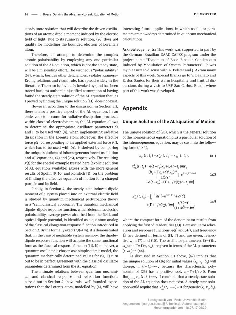
The unique solution of (26), which is the general solution of the homogeneous equation plus a particular solution of the inhomogeneous equation, may be cast into the follow-ing form (t ≥ t0),

= +h pAL 0 AL 0 AL 0( , ) ( , ) ( , ),x t t x t t x t t (a1)

Γ τ

φ χ

Γ Ω τ

Ω τφ Γ τ χ

− +

= − + −+ +

− −+

+ − + + −

0

hAL 0 0 0 0 0

2 2( )( 1/ )0 0 0

2 2

0 0

( , ) ( ) i ( )( )

[ e1 4

( ) ( 1 / )i ( ) ]

t t

x t t t t x t t mvb v x

t t t t m

(a2)

Γ τ φ

τΓ τ χ

Ω τ

− ′ +′ ′= − +′−′+ +

+

∫

0p ( 1/ )AL 0 0

2 2

( , ) d [ e ( )( )( 1 / )i ( ) ] ,

(1 4 )

t t tx t t t tf t tt m

m

(a3)

where the compact form of the denominator results from applying the first of its identities (33). Here oscillator relax-ation and response functions, φ(t) and χ(t), and frequency Ω are defined in terms of (Ω, Γ) and are given, respec-tively, in (7) and (10). The oscillator parameters Ω = Ω(τ, ω0) and Γ = Γ(τ, ω0) are given in terms of the AL parameters (τ, ω0) in (44).

As discussed in Section 3.3 above, (a2) implies that the unique solution of (26) for initial values (x0, v0, b0) will diverge, if (t − t0)→ ∞, because the characteristic poly-nomial of (26) has a positive root, z2 = Γ + 1/τ > 0. From

→−∞ = ∞0 AL 0lim ( , ) ,t x t t I conclude that a steady-state solu-

tion of the AL equation does not exist. A steady-state solu-tion would require that − ∞ =h

AL( , ) 0x t for generic (x0, v0, b0).




Fourier–Laplace Transform (FLT)

In (13), the Fourier–Laplace transform (FLT) of a bounded function f(t) (|f(t) | ≤ M < ∞) has been introduced

Θ

∞

−∞= = ℑ ≠∫ i( ) d e i ( ) ( ), sign [ ] 0,tzf z t s st f t s z

(a4)

which is an analytical function for all complex z outside the real axis. The FLT of f(t) has as a Cauchy integral representation

ωω ωω ω

π ω

= ±∞

−∞

′′ ′ ′′= → ±−∫

id ( )( ) ( ) i ( )z off z f f

z (a5)

with ω ω ω′′ = + − − 1( ) [ ( i ) ( i )]2i

f f o f o denoting the spec-

tral function, or dissipative part of ω+( i ),f o and ω ω ω′ = + + − 1( ) [ ( i ) ( i )]

2f f o f o denoting the reactive part

of ω+( i ).f o Dissipative and reactive parts obey disper-sion relations

d ( ) ( ) ,ff ω ωω

π ω ω

∞

−∞

′= − −′′−∫d ( )( ) , f ′′f ω ω

ωπ ω ω

∞

−∞

= −′−∫

(a6)

known as Kramers–Kronig relations in physics’ literature.

In general, d ( )( ) , f ′′f ω ωω

π ω ω

∞

−∞

= −′−∫ and d ( )( ) ff ω ω

ωπ ω ω

∞

−∞

′= − −′′−∫

d ( )( ) ff ω ωω

π ω ω

∞

−∞

′= − −′′−∫ will be complex functions of the real vari-

able ω. Functions f(t), which vanish for large |t | (as is the case for response and relaxation functions discussed above), are related to their spectral function by conven-tional Fourier transform

ω ωω

ω ωπ

∞ ∞ −

−∞ −∞′′ ′′= =∫ ∫i id d( ) e ( ), ( ) e ( ),

2t ttf f t f t f

(a7)

and one easily verifies for the response function χ(t) (7), which is purely imaginary, odd in t, and vanishing for |t | → ∞

χ ω χ ω χ ω χ ω ∗′′ ′′ ′′= ±ℑ ± = − − =( ) [ ( i )] ( ) ( ) ,o (a8)

a spectral function which is real, odd in ω, and 1/2 of the conventional Fourier transform of χ(t). Similarly, the

relaxation function φ(t) (7), which is real, even in t, and vanishing for |t | → ∞, will have a spectral function

φ ω φ ω φ ω φ ω ∗′′ ′′ ′′= ±ℑ ± = − =( ) [ ( i )] ( ) ( )o (a9)

which is real, even in ω, and just 1/2 of the conventional Fourier transform of φ(t). For response and relaxa-tion spectrum, Kubo’s identity takes the simple form: χ″(ω) = ωφ″(ω)/(mΩ2).

References[1] R. Grimm, M. Weidemüller, and Y. Ovchinnikov, Adv. At. Mol.

Opt. Phys. 42, 95 (2000).[2] G. Gilbert, A. Aspect, and C. Fabre, Introduction to Quantum

Optics, Campridge University Press, New York 2010.[3] L. Bergmann and Cl. Schaefer. Lehrbuch der Experimental-

physik, volume II (Elektrizitätslehre). Walter de Gruyter & Co., Berlin 1961.

[4] P. C. Martin. In C. de Witt and R. Balian, (eds, Problème à N Corps, page 37 ff), Gordon and Breach, New York 1968.

[5] D. J. Griffiths, Introduction to Electrodynamics, 3rd ed., Prentice-Hall Inc. 1999.

[6] J. D. Jackson, Classical Electrodynamics, 3rd ed., John Wiley & Sons Inc., New York 1999.

[7] J. D. Jackson, Classical Electrodynamics, 1st ed., John Wiley & Sons, New York 1962.

[8] P. A. M. Dirac, Math Phys Sci. 167, 148 (1938).[9] H. Spohn, Dynamics of Charged Particles and their

Radiation Field, Cambridge University Press, Cambridge, UK 2004.

[10] H. Spohn, Europhys. Lett. 50, 287 (2000).[11] F. Rohrlich, Phys. Lett A. 283, 276 (2001).[12] L. Landau and E. M. Lifshitz, The Classical Theory of Fields,

Pergamon Press, New York 1975.[13] G. W. Ford and R. F. O’Connell, Phys. Lett A. 157,

217 (1991).[14] O. Keller, Quantum Theory of Near-Field Electrodynamics,

Springer-Verlag, Heidelberg 2011.[15] J. M. Aguirregabiria, J. Phys. A: Math. Gen. 30, 2391

(1997).[16] W. Heitler, The Quantum Theory of Radiation, 3rd ed., Oxford

University Press, London 1954.



jürgen bosse* lorentz atom revisited by solving the

Documents