knowledge discovery in databases - dbs.ifi.uni-heidelberg.de · knowledge discovery in databases...
TRANSCRIPT
Knowledge Discovery in Databases
Erich Schubert
Winter Semester 2017/18
Part III
Clustering
Clustering Basic Concepts and Applications 3: 1 / 153
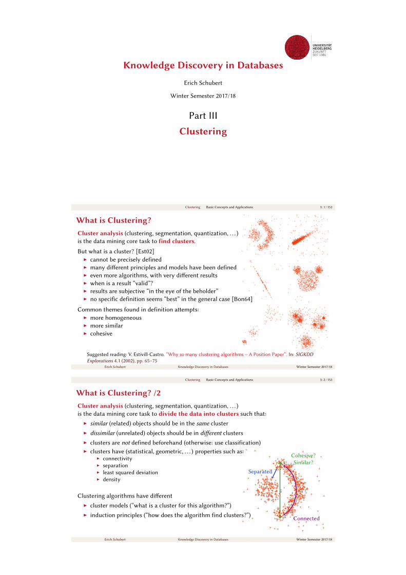
What is Clustering?Cluster analysis (clustering, segmentation, quantization, . . . )
is the data mining core task to find clusters.
But what is a cluster? [Est02]
I cannot be precisely defined
I many dierent principles and models have been defined
I even more algorithms, with very dierent results
I when is a result “valid”?
I results are subjective “in the eye of the beholder”
I no specific definition seems “best” in the general case [Bon64]
Common themes found in definition aempts:
I more homogeneous
I more similar
I cohesive
Suggested reading: V. Estivill-Castro. “Why so many clustering algorithms – A Position Paper”. In: SIGKDDExplorations 4.1 (2002), pp. 65–75
Erich Schubert Knowledge Discovery in Databases Winter Semester 2017/18
Clustering Basic Concepts and Applications 3: 2 / 153
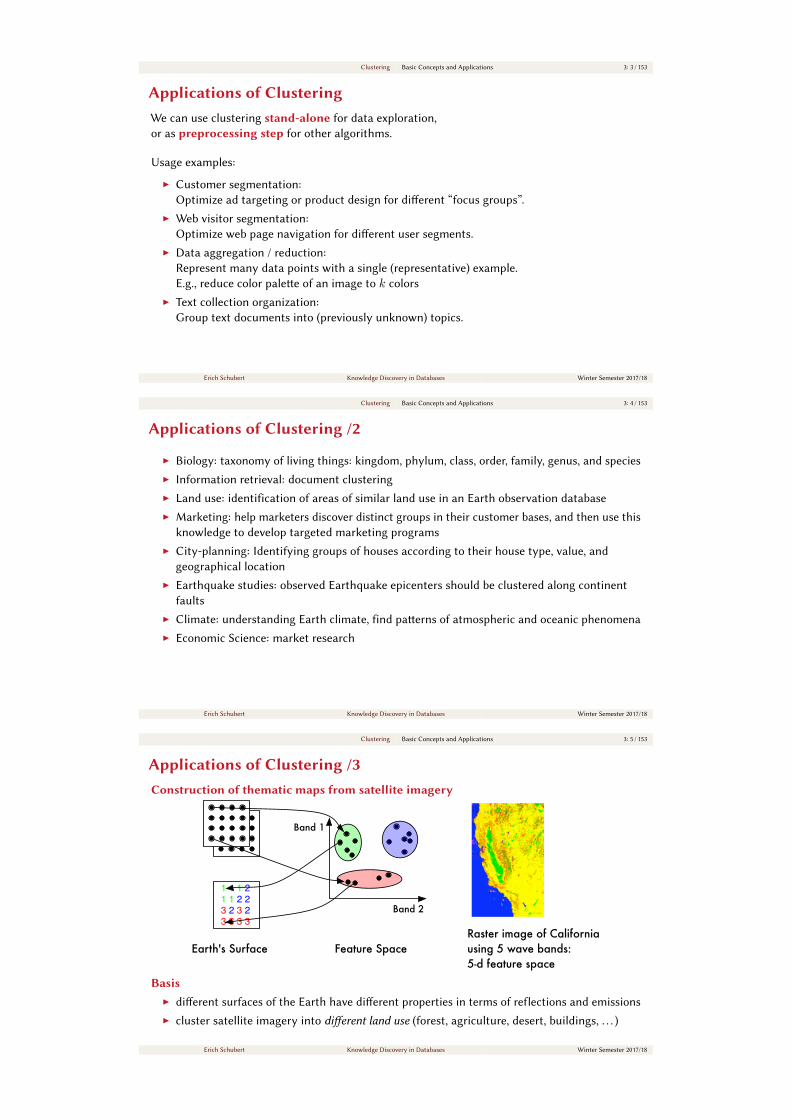
What is Clustering? /2Cluster analysis (clustering, segmentation, quantization, . . . )
is the data mining core task to divide the data into clusters such that:
I similar (related) objects should be in the same cluster
I dissimilar (unrelated) objects should be in dierent clusters
I clusters are not defined beforehand (otherwise: use classification)
I clusters have (statistical, geometric, . . . ) properties such as:
I connectivity
I separation
I least squared deviation
I density
Clustering algorithms have dierent
I cluster models (“what is a cluster for this algorithm?”)
I induction principles (“how does the algorithm find clusters?”)
Separated
Cohesive?
Similar?
Connected
Erich Schubert Knowledge Discovery in Databases Winter Semester 2017/18
Clustering Basic Concepts and Applications 3: 3 / 153
Applications of ClusteringWe can use clustering stand-alone for data exploration,
or as preprocessing step for other algorithms.
Usage examples:
I Customer segmentation:
Optimize ad targeting or product design for dierent “focus groups”.
I Web visitor segmentation:
Optimize web page navigation for dierent user segments.
I Data aggregation / reduction:
Represent many data points with a single (representative) example.
E.g., reduce color palee of an image to k colors
I Text collection organization:
Group text documents into (previously unknown) topics.
Erich Schubert Knowledge Discovery in Databases Winter Semester 2017/18
Clustering Basic Concepts and Applications 3: 4 / 153
Applications of Clustering /2
I Biology: taxonomy of living things: kingdom, phylum, class, order, family, genus, and species
I Information retrieval: document clustering
I Land use: identification of areas of similar land use in an Earth observation database
I Marketing: help marketers discover distinct groups in their customer bases, and then use this
knowledge to develop targeted marketing programs
I City-planning: Identifying groups of houses according to their house type, value, and
geographical location
I Earthquake studies: observed Earthquake epicenters should be clustered along continent
faults
I Climate: understanding Earth climate, find paerns of atmospheric and oceanic phenomena
I Economic Science: market research
Erich Schubert Knowledge Discovery in Databases Winter Semester 2017/18
Clustering Basic Concepts and Applications 3: 5 / 153
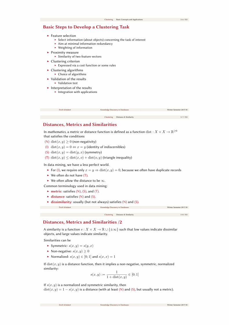
Applications of Clustering /3Construction of thematic maps from satellite imagery
1 1 1 21 1 2 23 2 3 23 3 3 3
Earth's Surface Feature Space
Band 2
Band 1
Raster image of Californiausing 5 wave bands:5-d feature space
BasisI dierent surfaces of the Earth have dierent properties in terms of reflections and emissions
I cluster satellite imagery into dierent land use (forest, agriculture, desert, buildings, . . . )
Erich Schubert Knowledge Discovery in Databases Winter Semester 2017/18
Clustering Basic Concepts and Applications 3: 6 / 153
Basic Steps to Develop a Clustering Task
I Feature selection
I Select information (about objects) concerning the task of interest
I Aim at minimal information redundancy
I Weighting of information
I Proximity measure
I Similarity of two feature vectors
I Clustering criterion
I Expressed via a cost function or some rules
I Clustering algorithms
I Choice of algorithms
I Validation of the results
I Validation test
I Interpretation of the results
I Integration with applications
Erich Schubert Knowledge Discovery in Databases Winter Semester 2017/18
Clustering Distance & Similarity 3: 7 / 153
Distances, Metrics and SimilaritiesIn mathematics, a metric or distance function is defined as a function dist : X ×X → R≥0
that satisfies the conditions
(N) dist(x, y) ≥ 0 (non-negativity)
(I) dist(x, y) = 0⇔ x = y (identity of indiscernibles)
(S) dist(x, y) = dist(y, x) (symmetry)
(T) dist(x, y) ≤ dist(x, o) + dist(o, y) (triangle inequality)
In data mining, we have a less perfect world.
I For (I), we require only x = y ⇒ dist(x, y) = 0, because we oen have duplicate records
I We oen do not have (T).
I We oen allow the distance to be∞.
Common terminology used in data mining:
I metric: satisfies (N), (S), and (T).
I distance: satisfies (N) and (S).
I dissimilarity: usually (but not always) satisfies (N) and (S).
Erich Schubert Knowledge Discovery in Databases Winter Semester 2017/18
Clustering Distance & Similarity 3: 8 / 153
Distances, Metrics and Similarities /2A similarity is a function s : X ×X → R ∪ ±∞ such that low values indicate dissimilar
objects, and large values indicate similarity.
Similarities can be
I Symmetric: s(x, y) = s(y, x)
I Non-negative: s(x, y) ≥ 0
I Normalized: s(x, y) ∈ [0; 1] and s(x, x) = 1
If dist(x, y) is a distance function, then it implies a non-negative, symmetric, normalized
similarity:
s(x, y) :=1
1 + dist(x, y)∈ [0; 1]
If s(x, y) is a normalized and symmetric similarity, then
dist(x, y) = 1− s(x, y) is a distance (with at least (N) and (S), but usually not a metric).
Erich Schubert Knowledge Discovery in Databases Winter Semester 2017/18
Clustering Distance & Similarity 3: 9 / 153
Distance FunctionsThere are many dierent distance functions.
The “standard” distance on Rd is Euclidean distance:
dEuclidean(x, y) =
√∑d(xd − yd)2 = ‖x− y‖2
Manhaan distance (city block metric):
dManhattan(x, y) =∑
d|xd − yd| = ‖x− y‖1
are special cases of Minkowski norms (Lp distances, p ≥ 1):
dLp(x, y) =(∑
d|xd − yd|p
)1/p= ‖x− y‖p
In the limit p→∞ we also get the maximum norm:
dMaximum(x, y) = maxd |xd − yd|
‖x‖ without index usually
refers to the Euclidean norm.
z many more distance functions – see the “Encyclopedia of Distances” [DD09]!
Erich Schubert Knowledge Discovery in Databases Winter Semester 2017/18
Clustering Distance & Similarity 3: 10 / 153
Distance Functions /2Many more variants:
Squared Euclidean distance (“sum of squares”):
d2Euclidean(x, y) =
∑d(xd − yd)2 = ‖x− y‖22
Minimum distance (p→ 0) – not metric:
dMinimum(x, y) = mind |xd − yd|Weighted minkowski norms:
dLp(x, y, ω) =(∑
dωd|xd − yd|p
)1/p
Canberra distance:
dCanberra(x, y) =∑
d
|xd − yd||xd|+ |yd|
z many more distance functions – see the “Encyclopedia of Distances” [DD09]!
Erich Schubert Knowledge Discovery in Databases Winter Semester 2017/18
Clustering Distance & Similarity 3: 11 / 153
Similarity FunctionsInstead of distances, we can oen also use similarities:
Cosine similarity:
scos(x, y) :=x · y‖x‖ · ‖y‖
=∑i xiyi√∑
i x2i ·√∑
i y2i
on data normalized to L2 length ‖x‖ = ‖y‖ = 1, this simplifies to:
scos(x, y) :=‖x‖=‖y‖=1
x · y =∑
ixiyi
Popular transformations to distances:
dcos1(x, y) = 1− scos(x, y)
dcos2(x, y) = arccos(scos(x, y))
zCareful: if we use similarities, large values are beer
– with distances, small values are beer.
Erich Schubert Knowledge Discovery in Databases Winter Semester 2017/18
Clustering Distance & Similarity 3: 12 / 153
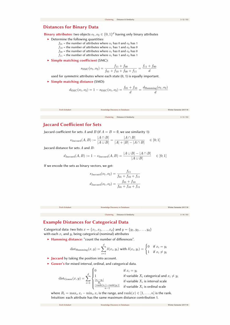
Distances for Binary DataBinary aributes: two objects o1, o2 ∈ 0, 1d having only binary aributes
I Determine the following quantities:
f01 = the number of aributes where o1 has 0 and o2 has 1
f10 = the number of aributes where o1 has 1 and o2 has 0
f00 = the number of aributes where o1 has 0 and o2 has 0
f11 = the number of aributes where o1 has 1 and o2 has 1
I Simple matching coeicient (SMC):
sSMC(o1, o2) =f11 + f00
f01 + f10 + f00 + f11=f11 + f00
d
used for symmetric aributes where each state (0, 1) is equally important.
I Simple matching distance (SMD):
dSMC(o1, o2) = 1− sSMC(o1, o2) =f01 + f10
d=dHamming(o1, o2)
d
Erich Schubert Knowledge Discovery in Databases Winter Semester 2017/18
Clustering Distance & Similarity 3: 13 / 153
Jaccard Coeicient for SetsJaccard coeicient for sets A and B (if A = B = ∅, we use similarity 1):
sJaccard(A,B) :=|A ∩B||A ∪B|
=|A ∩B|
|A|+ |B| − |A ∩B|∈ [0; 1]
Jaccard distance for sets A and B:
dJaccard(A,B) := 1− sJaccard(A,B) =|A ∪B| − |A ∩B|
|A ∪B|∈ [0; 1]
If we encode the sets as binary vectors, we get:
sJaccard(o1, o2) =f11
f01 + f10 + f11
dJaccard(o1, o2) =f01 + f10
f01 + f10 + f11
Erich Schubert Knowledge Discovery in Databases Winter Semester 2017/18
Clustering Distance & Similarity 3: 14 / 153
Example Distances for Categorical DataCategorical data: two lists x = x1, x2, . . . , xd and y = y1, y2, . . . , ydwith each xi and yi being categorical (nominal) aributes
I Hamming distance: “count the number of dierences”.
distHamming(x, y) =d∑i=1
δ(xi, yi) with δ(xi, yi) =
0 if xi = yi
1 if xi 6= yi
I Jaccard by taking the position into account.
I Gower’s for mixed interval, ordinal, and categorical data.
distGower(x, y) =d∑i=1
0 if xi = yi
1 if variable Xi categorical and xi 6= yi|xi−yi|Ri
if variable Xi is interval scale
| rank(xi)−rank(yi)|n−1 if variable Xi is ordinal scale
where Ri = maxx xi −minx xi is the range, and rank(x) ∈ [1, . . . , n] is the rank.
Intuition: each aribute has the same maximum distance contribution 1.
Erich Schubert Knowledge Discovery in Databases Winter Semester 2017/18
Clustering Distance & Similarity 3: 15 / 153
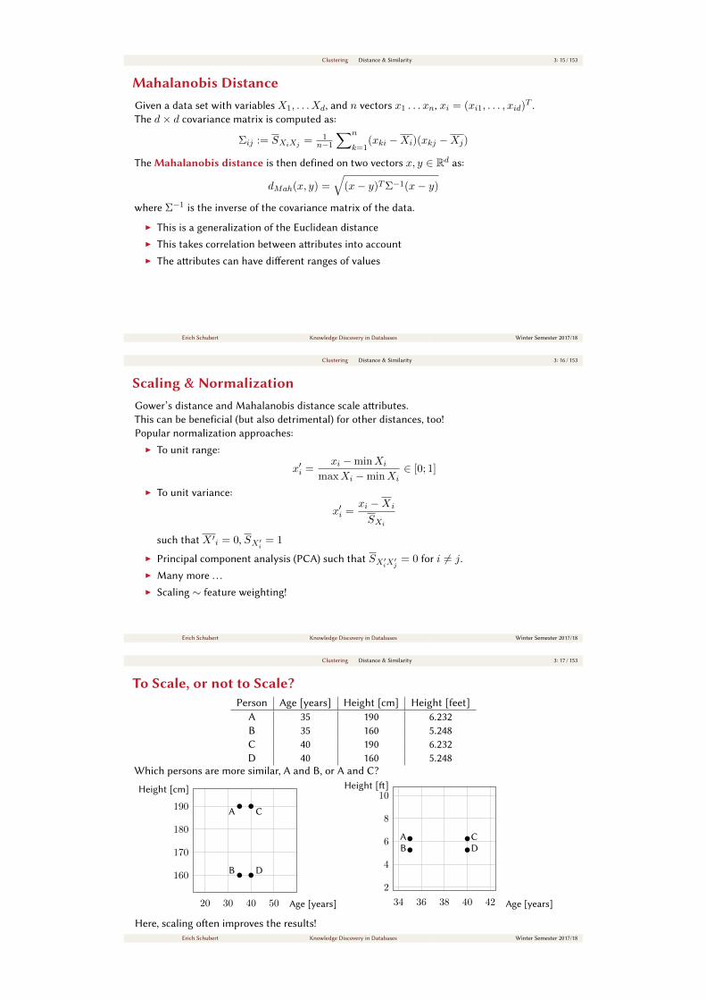
Mahalanobis DistanceGiven a data set with variables X1, . . . Xd, and n vectors x1 . . . xn, xi = (xi1, . . . , xid)
T.
The d× d covariance matrix is computed as:
Σij := SXiXj = 1n−1
∑n
k=1(xki −Xi)(xkj −Xj)
The Mahalanobis distance is then defined on two vectors x, y ∈ Rd as:
dMah(x, y) =√
(x− y)TΣ−1(x− y)
where Σ−1is the inverse of the covariance matrix of the data.
I This is a generalization of the Euclidean distance
I This takes correlation between aributes into account
I The aributes can have dierent ranges of values
Erich Schubert Knowledge Discovery in Databases Winter Semester 2017/18
Clustering Distance & Similarity 3: 16 / 153
Scaling & NormalizationGower’s distance and Mahalanobis distance scale aributes.
This can be beneficial (but also detrimental) for other distances, too!
Popular normalization approaches:
I To unit range:
x′i =xi −minXi
maxXi −minXi∈ [0; 1]
I To unit variance:
x′i =xi −Xi
SXi
such that X ′i = 0, SX′i = 1
I Principal component analysis (PCA) such that SX′iX′j = 0 for i 6= j.
I Many more . . .
I Scaling ∼ feature weighting!
Erich Schubert Knowledge Discovery in Databases Winter Semester 2017/18
Clustering Distance & Similarity 3: 17 / 153
To Scale, or not to Scale?Person Age [years] Height [cm] Height [feet]
A 35 190 6.232
B 35 160 5.248
C 40 190 6.232
D 40 160 5.248
Which persons are more similar, A and B, or A and C?
A
B
C
D
20 30 40 50 Age [years]
160
170
180
190
Height [cm]
A
B
C
D
34 36 38 40 42 Age [years]
2
4
6
8
10Height []
Here, scaling oen improves the results!
Erich Schubert Knowledge Discovery in Databases Winter Semester 2017/18
Clustering Distance & Similarity 3: 18 / 153
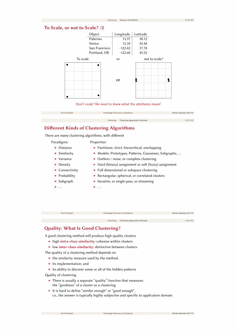
To Scale, or not to Scale? /2Object Longitude Latitude
Palermo 13.37 38.12
Venice 12.34 45.44
San Francisco -122.42 37.78
Portland, OR -122.68 45.52
To scale or not to scale?
or
Don’t scale! We need to know what the aributes mean!
Erich Schubert Knowledge Discovery in Databases Winter Semester 2017/18
Clustering Clustering Approaches Overview 3: 19 / 153
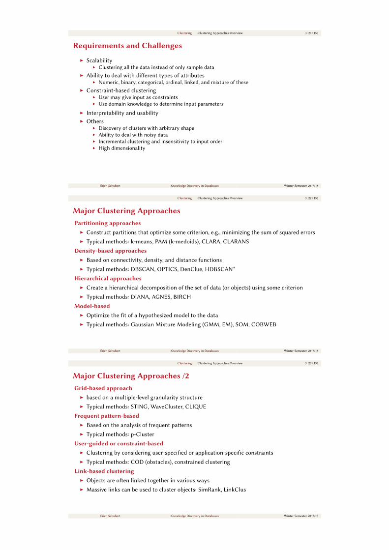
Dierent Kinds of Clustering AlgorithmsThere are many clustering algorithms, with dierent
Paradigms:
I Distance
I Similarity
I Variance
I Density
I Connectivity
I Probability
I Subgraph
I . . .
Properties:
I Partitions: strict, hierarchical, overlapping
I Models: Prototypes, Paerns, Gaussians, Subgraphs, . . .
I Outliers / noise, or complete clustering
I Hard (binary) assignment or so (fuzzy) assignment
I Full dimensional or subspace clustering
I Rectangular, spherical, or correlated clusters
I Iterative, or single-pass, or streaming
I . . .
Erich Schubert Knowledge Discovery in Databases Winter Semester 2017/18
Clustering Clustering Approaches Overview 3: 20 / 153
ality: What Is Good Clustering?A good clustering method will produce high quality clusters
I high intra-class similarity: cohesive within clusters
I low inter-class similarity: distinctive between clusters
The quality of a clustering method depends on
I the similarity measure used by the method,
I its implementation, and
I its ability to discover some or all of the hidden paerns
ality of clustering
I There is usually a separate “quality” function that measures
the “goodness” of a cluster or a clustering
I It is hard to define “similar enough” or “good enough”,
i.e., the answer is typically highly subjective and specific to application domain
Erich Schubert Knowledge Discovery in Databases Winter Semester 2017/18
Clustering Clustering Approaches Overview 3: 21 / 153
Requirements and Challenges
I Scalability
I Clustering all the data instead of only sample data
I Ability to deal with dierent types of aributes
I Numeric, binary, categorical, ordinal, linked, and mixture of these
I Constraint-based clustering
I User may give input as constraints
I Use domain knowledge to determine input parameters
I Interpretability and usability
I Others
I Discovery of clusters with arbitrary shape
I Ability to deal with noisy data
I Incremental clustering and insensitivity to input order
I High dimensionality
Erich Schubert Knowledge Discovery in Databases Winter Semester 2017/18
Clustering Clustering Approaches Overview 3: 22 / 153
Major Clustering ApproachesPartitioning approaches
I Construct partitions that optimize some criterion, e.g., minimizing the sum of squared errors
I Typical methods: k-means, PAM (k-medoids), CLARA, CLARANS
Density-based approachesI Based on connectivity, density, and distance functions
I Typical methods: DBSCAN, OPTICS, DenClue, HDBSCAN*
Hierarchical approachesI Create a hierarchical decomposition of the set of data (or objects) using some criterion
I Typical methods: DIANA, AGNES, BIRCH
Model-basedI Optimize the fit of a hypothesized model to the data
I Typical methods: Gaussian Mixture Modeling (GMM, EM), SOM, COBWEB
Erich Schubert Knowledge Discovery in Databases Winter Semester 2017/18
Clustering Clustering Approaches Overview 3: 23 / 153
Major Clustering Approaches /2Grid-based approach
I based on a multiple-level granularity structure
I Typical methods: STING, WaveCluster, CLIQUE
Frequent paern-basedI Based on the analysis of frequent paerns
I Typical methods: p-Cluster
User-guided or constraint-basedI Clustering by considering user-specified or application-specific constraints
I Typical methods: COD (obstacles), constrained clustering
Link-based clusteringI Objects are oen linked together in various ways
I Massive links can be used to cluster objects: SimRank, LinkClus
Erich Schubert Knowledge Discovery in Databases Winter Semester 2017/18
Clustering Hierarchical Methods 3: 24 / 153
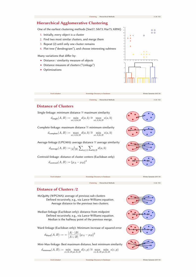
Hierarchical Agglomerative ClusteringOne of the earliest clustering methods [Sne57; Sib73; Har75; KR90]:
1. Initially, every object is a cluster
2. Find two most similar clusters, and merge them
3. Repeat (2) until only one cluster remains
4. Plot tree (“dendrogram”), and choose interesting subtrees
Many variations that dier by:
I Distance / similarity measure of objectsI Distance measure of clusters (“Linkage”)
I Optimizations
0 1 2 3 4 5 6 7 8 9 10 11 120
1
2
3
4
5
6
7
8
9
10
11
12
0
1
2
3
4
Erich Schubert Knowledge Discovery in Databases Winter Semester 2017/18
Clustering Hierarchical Methods 3: 25 / 153
Distance of ClustersSingle-linkage: minimum distance
∼= maximum similarity
dsingle(A,B) := mina∈A,b∈B
d(a, b) ∼= maxa∈A,b∈B
s(a, b)
Complete-linkage: maximum distance∼= minimum similarity
dcomplete(A,B) := maxa∈A,b∈B
d(a, b) ∼= mina∈A,b∈B
s(a, b)
Average-linkage (UPGMA): average distance∼= average similarity
daverage(A,B) := 1|A|·|B|
∑a∈A
∑b∈B
d(a, b)
Centroid-linkage: distance of cluster centers (Euclidean only)
dcentroid(A,B) := ‖µA − µB‖2
Erich Schubert Knowledge Discovery in Databases Winter Semester 2017/18
Clustering Hierarchical Methods 3: 26 / 153
Distance of Clusters /2Mciy (WPGMA): average of previous sub-clusters
Defined recursively, e.g., via Lance-Williams equation.
Average distance to the previous two clusters.
Median-linkage (Euclidean only): distance from midpoint
Defined recursively, e.g., via Lance-Williams equation.
Median is the halfway point of the previous merge.
Ward-linkage (Euclidean only): Minimum increase of squared error
dWard(A,B) := =|A| · |B||A ∪B|
‖µA − µB‖2
Mini-Max-linkage: Best maximum distance, best minimum similarity
dminimax(A,B) := minc∈A∪B
maxp∈A∪B
d(c, p) ∼= maxc∈A∪B
minp∈A∪B
s(c, p)
Erich Schubert Knowledge Discovery in Databases Winter Semester 2017/18
Clustering Hierarchical Methods 3: 27 / 153
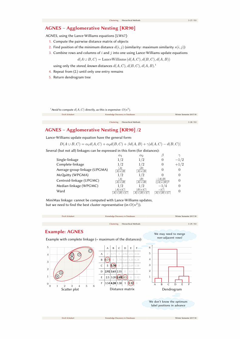
AGNES – Agglomerative Nesting [KR90]AGNES, using the Lance-Williams equations [LW67]:
1. Compute the pairwise distance matrix of objects
2. Find position of the minimum distance d(i, j) (similarity: maximum similarity s(i, j))
3. Combine rows and columns of i and j into one using Lance-Williams update equations
d(A ∪B,C) = LanceWilliams (d(A,C), d(B,C), d(A,B))
using only the stored, known distances d(A,C), d(B,C), d(A,B).1
4. Repeat from (2.) until only one entry remains
5. Return dendrogram tree
1Avoid to compute d(A,C) directly, as this is expensive: O(n2).
Erich Schubert Knowledge Discovery in Databases Winter Semester 2017/18
Clustering Hierarchical Methods 3: 28 / 153
AGNES – Agglomerative Nesting [KR90] /2Lance-Williams update equation have the general form:
D(A ∪B,C) = α1d(A,C) + α2d(B,C) + βd(A,B) + γ|d(A,C)− d(B,C)|
Several (but not all) linkages can be expressed in this form (for distances):
α1 α2 β γSingle-linkage 1/2 1/2 0 −1/2Complete-linkage 1/2 1/2 0 +1/2
Average-group-linkage (UPGMA)|A|
|A|+|B||B|
|A|+|B| 0 0
Mciy (WPGMA) 1/2 1/2 0 0
Centroid-linkage (UPGMC)|A|
|A|+|B||B|
|A|+|B|−|A||B|(|A|+|B|)2 0
Median-linkage (WPGMC) 1/2 1/2 −1/4 0
Ward|A|+|C|
|A|+|B|+|C||B|+|C|
|A|+|B|+|C|−|C|
|A|+|B|+|C| 0
MiniMax linkage: cannot be computed with Lance-Williams updates,
but we need to find the best cluster representative (in O(n2)).
Erich Schubert Knowledge Discovery in Databases Winter Semester 2017/18
Clustering Hierarchical Methods 3: 29 / 153
Example: AGNESExample with complete linkage (= maximum of the distances):
Scaer plot
A
B
C
D
E
F
0 1 2 3 4 5 60
1
2
3
4
5
Distance matrix
A B C D E F
A
B
C
D
E
F
0
0
0
0
0
0
0.71
0.71
5
5
2.92
2.92
2.5
2.5
3.54
3.54
5.70
5.70
3.61
3.61
3.20
3.20
4.24
4.24
2.55
2.55
2.69
2.69
1.58
1.58
0.5
0.5
1
1
1.12
1.12
2.92
2.5
3.61
3.20
2.55
2.69 0.5
1 1.12
2.92 3.61
2.69
1.12
0.71
5 5.70
3.54 4.24
5.70
4.24 1.584.24
2.69
5.70
Dendrogram
A B C D E F
1
2
3
4
5
6
We may need to merge
non-adjacent rows!
We don’t know the optimum
label positions in advance
Erich Schubert Knowledge Discovery in Databases Winter Semester 2017/18

Clustering Hierarchical Methods 3: 30 / 153
Example: AGNES /2Example with single linkage (= minimum of the distances):
Scaer plot
A
B
C
D
E
F
0 1 2 3 4 5 60
1
2
3
4
5
Distance matrix
A B C D E F
A
B
C
D
E
F
0
0
0
0
0
0
0.71
0.71
5
5
2.92
2.92
2.5
2.5
3.54
3.54
5.70
5.70
3.61
3.61
3.20
3.20
4.24
4.24
2.55
2.55
2.69
2.69
1.58
1.58
0.5
0.5
1
1
1.12
1.12
2.92
2.5
3.61
3.20
2.55
2.69 0.5
1 1.12
3.202.5
2.55
1
0.71
5 5.70
3.54 4.24
5
3.54 1.58
2.5
1.58
2.5
Dendrogram
A B C D E F
0.5
1
1.5
2
2.5
3
In this very simple example,
single and complete linkage
are very similar
Same clusters in this example,
but this is usually not the case.
Erich Schubert Knowledge Discovery in Databases Winter Semester 2017/18
Clustering Hierarchical Methods 3: 31 / 153
Extracting Clusters from a DendrogramAt this point, we have the dendrogram – but not yet “clusters”.
Various strategies have been discussed:
I Visually inspect the dendrogram, choose interesting branches
I Stop when k clusters remain (may be necessary to ignore noise [Sch+17b])
I Stop at a certain distance (e.g., maximum cluster diameter with complete-link)
I Change in cluster sizes or density [Cam+13]
I Constraints satisfied (semi-supervised) [Pou+14]:
Certain objects are labeled as “must” or “should not” be in the same clusters.
0
1
2
3
4
Erich Schubert Knowledge Discovery in Databases Winter Semester 2017/18
Clustering Hierarchical Methods 3: 32 / 153
Complexity of Hierarchical ClusteringComplexity analysis of AGNES:
1. Computing the distance matrix: O(n2) time and memory.
2. Finding the minimum distance / maximum similarity: O(n2) · i3. Updating the matrix: O(n) · i (with Lance-Williams) or O(n2) · i4. Number of iterations: i = O(n)
Total: O(n3) time and O(n2) memory!
Beer algorithms can run in guaranteed O(n2) time [Sib73; Def77], with priority queues we get
O(n2 log n) [Mur83; DE84; Epp98; Mül11], or “usually n2” time with caching [And73].
Instead of agglomerative (boom-up), we can also begin with one cluster, and divide it (DIANA).
But there are O(2n) splits – need heuristics (i.e., other clustering algorithms) to split.
zHierarchical clustering does not scale to large data, code optimization maers [KSZ16].
Erich Schubert Knowledge Discovery in Databases Winter Semester 2017/18

Clustering Hierarchical Methods 3: 33 / 153
Benefits and Limitations of HACBenefits:
I Very general: any distance / similarity (for text: cosine!)
I Easy to understand and interpret
I Hierarchical result
I Dendrogram visualization oen useful (for small data)
I Number of clusters does not need to be fixed beforehand
I Many variants
Limitations:
I Scalability is the main problem (in particular, O(n2) memory)
I In many cases, users want a flat partitioning
I Unbalanced cluster sizes (i.e., number of points)
I Outliers
Erich Schubert Knowledge Discovery in Databases Winter Semester 2017/18
Clustering Partitioning Methods 3: 34 / 153
k-means ClusteringThe k-means problem:
I Divide data into k subsets (k is a parameter)
I Subsets represented by their arithmetic mean µCI Optimize the least squared error
SSQ :=∑C
∑d
∑xi∈C
(xi,d − µC,d)2
Important properties:
I Squared errors put more weight on larger deviations
I Arithmetic mean is the maximum likelihood estimator of centrality
I Data is split into Voronoi cells
z k-means is a good choice, if we have k signals and normal distributed measurement error
Suggested reading: the history of least squares estimation (Legendre, Gauss):
https://en.wikipedia.org/wiki/Least_squares#History
Erich Schubert Knowledge Discovery in Databases Winter Semester 2017/18
Clustering Partitioning Methods 3: 35 / 153
The Sum of Squares ObjectiveThe sum-of-squares objective:
SSQ :=∑
C︸ ︷︷ ︸every cluster
∑d︸︷︷︸
× every dimension×
∑xi∈C︸ ︷︷ ︸
every point
(xi,d − µC,d)2︸ ︷︷ ︸squared deviation from mean
For every cluster C and dimension d, the arithmetic mean minimizes∑xi∈C
(xi,d − µC,d)2is minimized by µC,d = 1
|C|
∑xi∈C
xi,d
Assigning every point xi to its least-squares closest cluster C usually2
reduces SSQ, too.
Note: sum of squares ≡ squared Euclidean distance:∑d(xi,d − µC,d)2 ≡ ‖xi − µC‖2 ≡ d2
Euclidean(xi, µC)
We can therefore say that every point is assigned the “closest” cluster, but we cannot use arbitrary
other distance functions in k-means (because the arithmetic mean only minimizes SSQ).
We can rearrange these sums
because of communtativity
2
This is not always optimal: the change in mean can increase the SSQ of the new cluster.
But this dierence is commonly ignored in algorithms and textbooks.
Erich Schubert Knowledge Discovery in Databases Winter Semester 2017/18
Clustering Partitioning Methods 3: 36 / 153
The Standard Algorithm (Lloyd’s Algorithm)The standard algorithm for k-means [Ste56; For65; Llo82]:
Algorithm: Lloyd-Forgy algorithm for k-means
1 Choose k points randomly as initial centers
2 repeat3 Assign every point to the least-squares closest center
4 stop if no cluster assignment changed
5 Update the centers with the arithmetic mean
This is not the most eicient algorithm (despite everybody teaching this variant).
ELKI [Sch+15] contains ≈ 10 variants (e.g., Sort-Means [Phi02]; benchmarks in [KSZ16]).
There is lile reason to still use this variant in practise!
The name k-means was first used by Maceen for a slightly dierent algorithm [Mac67].
k-means was invented several times, and has an interesting history [Boc07].
Lines 3 and 5
both improve SSQLines 3 and 5
both improve SSQ
Erich Schubert Knowledge Discovery in Databases Winter Semester 2017/18
Clustering Partitioning Methods 3: 37 / 153
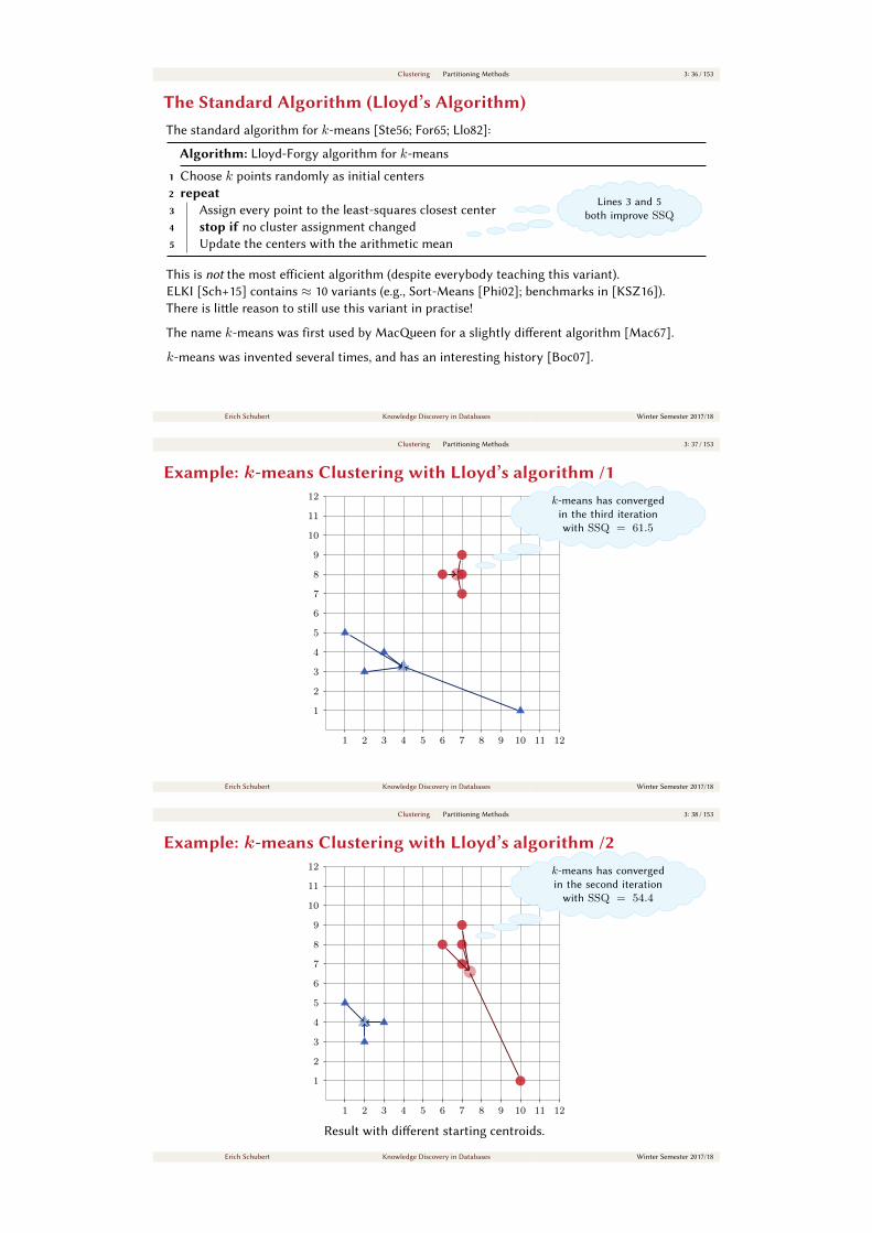
Example: k-means Clustering with Lloyd’s algorithm /1
1 2 3 4 5 6 7 8 9 10 11 12
1
2
3
4
5
6
7
8
9
10
11
12 k-means has converged
in the third iteration
with SSQ = 61.5
Erich Schubert Knowledge Discovery in Databases Winter Semester 2017/18
Clustering Partitioning Methods 3: 38 / 153
Example: k-means Clustering with Lloyd’s algorithm /2
1 2 3 4 5 6 7 8 9 10 11 12
1
2
3
4
5
6
7
8
9
10
11
12
Result with dierent starting centroids.
k-means has converged
in the second iteration
with SSQ = 54.4
Erich Schubert Knowledge Discovery in Databases Winter Semester 2017/18
Clustering Partitioning Methods 3: 39 / 153
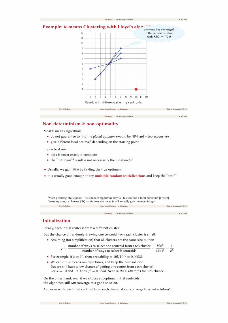
Example: k-means Clustering with Lloyd’s algorithm /3
1 2 3 4 5 6 7 8 9 10 11 12
1
2
3
4
5
6
7
8
9
10
11
12
Result with dierent starting centroids.
k-means has converged
in the second iteration
with SSQ = 72.9
Erich Schubert Knowledge Discovery in Databases Winter Semester 2017/18
Clustering Partitioning Methods 3: 40 / 153
Non-determinism & non-optimalityMost k-means algorithms
I do not guarantee to find the global optimum (would be NP-hard – too expensive)
I give dierent local optima,3
depending on the starting point
In practical use:
I data is never exact, or complete
I the “optimum”4
result is not necessarily the most useful
z Usually, we gain lile by finding the true optimum
z It is usually good enough to try multiple random initializations and keep the “best”4
3
More precisely: static point. The standard algorithm may fail to even find a local minimum [HW79].
4
Least squares, i.e., lowest SSQ – this does not mean it will actually give the most insight.
Erich Schubert Knowledge Discovery in Databases Winter Semester 2017/18
Clustering Partitioning Methods 3: 41 / 153
InitializationIdeally, each initial center is from a dierent cluster.
But the chance of randomly drawing one centroid from each cluster is small:
I Assuming (for simplification) that all clusters are the same size n, then
p =number of ways to select one centroid from each cluster
number of ways to select k centroids
=k!nk
(kn)k=k!
kk
I For example, if k = 10, then probability = 10!/1010 = 0.00036
I We can run k-means multiple times, and keep the best solution.
But we still have a low chance of geing one center from each cluster!
For k = 10 and 100 tries: p′ = 0.0353. Need ≈ 2000 aempts for 50% chance.
On the other hand, even if we choose suboptimal initial centroids,
the algorithm still can converge to a good solution.
And even with one initial centroid from each cluster, it can converge to a bad solution!
Erich Schubert Knowledge Discovery in Databases Winter Semester 2017/18
Clustering Partitioning Methods 3: 42 / 153
Initialization /2Several strategies for initializing k-means exist:
I Initial centers given by domain expert
I Randomly assign points to partitions 1 . . . k (not very good) [For65]
I Randomly generate k centers from a uniform distribution (not very good)
I Randomly choose k data points as centers (uniform from the data) [For65]
I First k data points [Mac67, incremental k-means]
I Choose a point randomly, then use always the farthest point to get k initial points
(oen quite well; initial centers are oen outliers, and gives similar results when run oen)
I Weighting points by their distance [AV07, K-means++]
Points are chosen randomly with p ∝ minc ‖xi − c‖2 (c = all current seeds)
I Run a few k-means iterations on a sample, then use centroids from the sample result.
I . . .
Erich Schubert Knowledge Discovery in Databases Winter Semester 2017/18
Clustering Partitioning Methods 3: 43 / 153
Complexity of k-means ClusteringIn the standard algorithm:
1. Initialization is usually cheap, O(k) (k-means++: O(N · k · d) [AV07])
2. Reassignment is O(N · k · d) · i3. Mean computation is O(N · d) · i4. Number of iterations i ∈ 2Ω(
√N)
[AV06] (but fortunately, usually i N )
5. Total: O(N · k · d · i)
Worst case is superpolynomial, but in practice the method will usually run much beer than n2.
We can force a limit on the number of iterations, e.g., i = 100, with lile loss in quality usually.
In practice, oen the fastest clustering algorithm we use.
Improved algorithms primarily reduce the number of computations for reassignment,
but usually with no theoretical guarantees (so still O(N · k · d) · i worst-case)
Erich Schubert Knowledge Discovery in Databases Winter Semester 2017/18
Clustering Partitioning Methods 3: 44 / 153
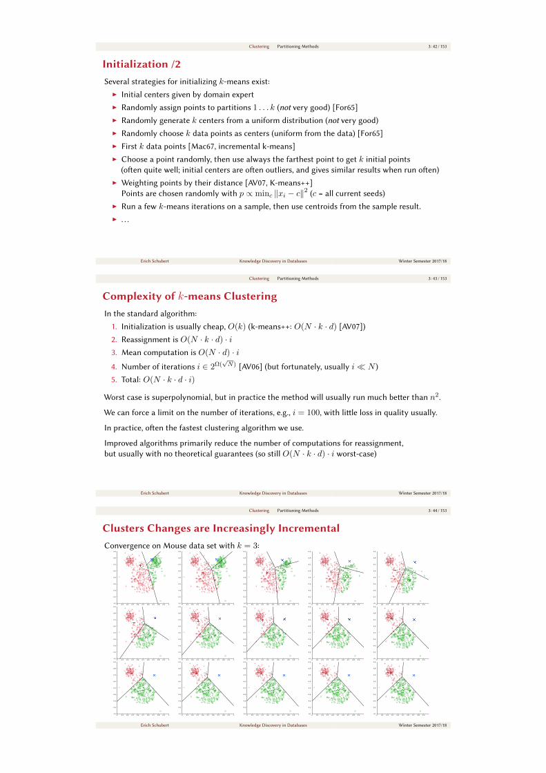
Clusters Changes are Increasingly IncrementalConvergence on Mouse data set with k = 3:
0 0.1 0.2 0.3 0.4 0.5 0.6 0.7 0.8 0.9 10.1
0.2
0.3
0.4
0.5
0.6
0.7
0.8
0.9
0 0.1 0.2 0.3 0.4 0.5 0.6 0.7 0.8 0.9 10.1
0.2
0.3
0.4
0.5
0.6
0.7
0.8
0.9
0 0.1 0.2 0.3 0.4 0.5 0.6 0.7 0.8 0.9 10.1
0.2
0.3
0.4
0.5
0.6
0.7
0.8
0.9
0 0.1 0.2 0.3 0.4 0.5 0.6 0.7 0.8 0.9 10.1
0.2
0.3
0.4
0.5
0.6
0.7
0.8
0.9
0 0.1 0.2 0.3 0.4 0.5 0.6 0.7 0.8 0.9 10.1
0.2
0.3
0.4
0.5
0.6
0.7
0.8
0.9
0 0.1 0.2 0.3 0.4 0.5 0.6 0.7 0.8 0.9 10.1
0.2
0.3
0.4
0.5
0.6
0.7
0.8
0.9
0 0.1 0.2 0.3 0.4 0.5 0.6 0.7 0.8 0.9 10.1
0.2
0.3
0.4
0.5
0.6
0.7
0.8
0.9
0 0.1 0.2 0.3 0.4 0.5 0.6 0.7 0.8 0.9 10.1
0.2
0.3
0.4
0.5
0.6
0.7
0.8
0.9
0 0.1 0.2 0.3 0.4 0.5 0.6 0.7 0.8 0.9 10.1
0.2
0.3
0.4
0.5
0.6
0.7
0.8
0.9
0 0.1 0.2 0.3 0.4 0.5 0.6 0.7 0.8 0.9 10.1
0.2
0.3
0.4
0.5
0.6
0.7
0.8
0.9
0 0.1 0.2 0.3 0.4 0.5 0.6 0.7 0.8 0.9 10.1
0.2
0.3
0.4
0.5
0.6
0.7
0.8
0.9
0 0.1 0.2 0.3 0.4 0.5 0.6 0.7 0.8 0.9 10.1
0.2
0.3
0.4
0.5
0.6
0.7
0.8
0.9
0 0.1 0.2 0.3 0.4 0.5 0.6 0.7 0.8 0.9 10.1
0.2
0.3
0.4
0.5
0.6
0.7
0.8
0.9
0 0.1 0.2 0.3 0.4 0.5 0.6 0.7 0.8 0.9 10.1
0.2
0.3
0.4
0.5
0.6
0.7
0.8
0.9
0 0.1 0.2 0.3 0.4 0.5 0.6 0.7 0.8 0.9 10.1
0.2
0.3
0.4
0.5
0.6
0.7
0.8
0.9
Erich Schubert Knowledge Discovery in Databases Winter Semester 2017/18
Clustering Partitioning Methods 3: 45 / 153
Benefits and Drawbacks of k-meansBenefits:
I Very fast algorithm (O(k · d ·N), if we limit the number of iterations)
I Convenient centroid vector for every cluster
(We can analyze this vector to get a “topic”)
I Can be run multiple times to get dierent results
Limitations:
I Diicult to choose the number of clusters, k
I Cannot be used with arbitrary distances
I Sensitive to scaling – requires careful preprocessing
I Does not produce the same result every time
I Sensitive to outliers (squared errors emphasize outliers)
I Cluster sizes can be quite unbalanced (e.g., one-element outlier clusters)
Erich Schubert Knowledge Discovery in Databases Winter Semester 2017/18
Clustering Partitioning Methods 3: 46 / 153
Choosing the “Optimum” k for k-meansA key challenge of k-means is choosing k:
I Trivial to prove: SSQoptimum,k ≥ SSQ
optimum,k+1.
z Avoid comparing SSQ for dierent k or dierent data (including normalization).
I SSQk=N = 0 — “perfect” solution? No: useless.
I SSQk may exhibit an “elbow” or “knee”: initially it improves fast, then much slower.
I Use alternate criteria such as Silhouee [Rou87], AIC [Aka77], BIC [Sch78; ZXF08].
z Computing silhouee is O(n2) – more expensive than k-means.
z AIC, BIC try to reduce overfiing by penalizing model complexity (= high k).
More details will come in evaluation section.
I Nevertheless, these measures are heuristics – other k can be beer in practice!
I Methods such as X-means [PM00] split clusters as long as a quality criterion improves.
Erich Schubert Knowledge Discovery in Databases Winter Semester 2017/18
Clustering Partitioning Methods 3: 47 / 153
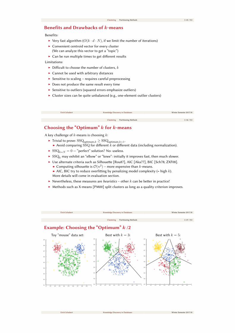
Example: Choosing the “Optimum” k /2Toy “mouse” data set:
0 0.1 0.2 0.3 0.4 0.5 0.6 0.7 0.8 0.9 10.1
0.2
0.3
0.4
0.5
0.6
0.7
0.8
0.9
Best with k = 3:
0 0.1 0.2 0.3 0.4 0.5 0.6 0.7 0.8 0.9 10.1
0.2
0.3
0.4
0.5
0.6
0.7
0.8
0.9
Best with k = 5:
0 0.1 0.2 0.3 0.4 0.5 0.6 0.7 0.8 0.9 10.1
0.2
0.3
0.4
0.5
0.6
0.7
0.8
0.9
Erich Schubert Knowledge Discovery in Databases Winter Semester 2017/18
Clustering Partitioning Methods 3: 47 / 153
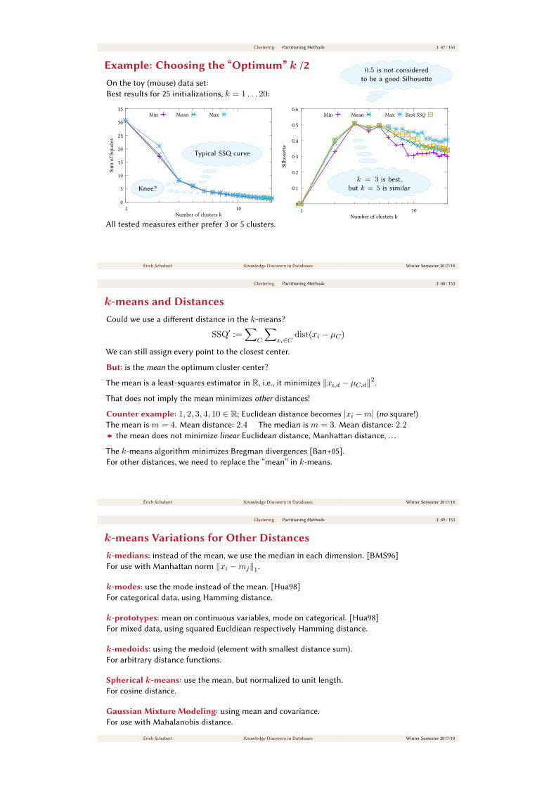
Example: Choosing the “Optimum” k /2On the toy (mouse) data set:
Best results for 25 initializations, k = 1 . . . 20:
0
5
10
15
20
25
30
35
1 10
Sum
of S
quar
es
Number of clusters k
Min Mean Max
0
0.1
0.2
0.3
0.4
0.5
0.6
1 10
Silh
oue
e
Number of clusters k
Min Mean Max Best SSQ
All tested measures either prefer 3 or 5 clusters.
Typical SSQ curve
Knee?Knee?
0.5 is not considered
to be a good Silhouee
k = 3 is best,
but k = 5 is similar
Erich Schubert Knowledge Discovery in Databases Winter Semester 2017/18
Clustering Partitioning Methods 3: 48 / 153
k-means and DistancesCould we use a dierent distance in the k-means?
SSQ′ :=∑
C
∑xi∈C
dist(xi − µC)
We can still assign every point to the closest center.
But: is the mean the optimum cluster center?
The mean is a least-squares estimator in R, i.e., it minimizes ‖xi,d − µC,d‖2.
That does not imply the mean minimizes other distances!
Counter example: 1, 2, 3, 4, 10 ∈ R; Euclidean distance becomes |xi −m| (no square!)
The mean is m = 4. Mean distance: 2.4 The median is m = 3. Mean distance: 2.2z the mean does not minimize linear Euclidean distance, Manhaan distance, . . .
The k-means algorithm minimizes Bregman divergences [Ban+05].
For other distances, we need to replace the “mean” in k-means.
Erich Schubert Knowledge Discovery in Databases Winter Semester 2017/18
Clustering Partitioning Methods 3: 49 / 153
k-means Variations for Other Distancesk-medians: instead of the mean, we use the median in each dimension. [BMS96]
For use with Manhaan norm ‖xi −mj‖1.
k-modes: use the mode instead of the mean. [Hua98]
For categorical data, using Hamming distance.
k-prototypes: mean on continuous variables, mode on categorical. [Hua98]
For mixed data, using squared Eucldiean respectively Hamming distance.
k-medoids: using the medoid (element with smallest distance sum).
For arbitrary distance functions.
Spherical k-means: use the mean, but normalized to unit length.
For cosine distance.
Gaussian Mixture Modeling: using mean and covariance.
For use with Mahalanobis distance.
Erich Schubert Knowledge Discovery in Databases Winter Semester 2017/18

Clustering Partitioning Methods 3: 50 / 153
k-means for Text ClusteringCosine similarity is closely connected to squared Euclidean distance.
Spherical k-means [DM01] uses:
I Input data is normalized to have ‖xi‖ = 1
I At each iteration, the new centers are normalized to µ′C := ‖µC‖ = 1
I µ′C minimizes average cosine similarity [DM01]∑xi∈C
⟨xi, µ
′C
⟩ ∼= |C| −∑xi∈C
∥∥xi, µ′C∥∥2
I Sparse nearest-centroid computations in O(d′) where d′ is the number of non-zero values
I Result is similar to a SVD factorization of the document-term-matrix [DM01]
Erich Schubert Knowledge Discovery in Databases Winter Semester 2017/18
Clustering Partitioning Methods 3: 51 / 153
Pre-processing and Post-processingPre-processing and post-processing commonly used with k-means:
Pre-processing:
I Scale / normalize continuous aributes to [0; 1] or unit variance.
I Encode categorical aributes as binary aributes.
I Eliminate outliers
Post-processing
I Eliminate clusters with few elements (probably outliers)
I Split “loose” clusters, i.e., clusters with relatively high SSE
I Merge clusters that are “close” and that have relatively low SSE
I Can use these steps during the clustering process
E.g., ISODATA algorithm [BH65], X-means [PM00], G-means [HE03]
Erich Schubert Knowledge Discovery in Databases Winter Semester 2017/18
Clustering Partitioning Methods 3: 52 / 153
Limitations of k-meansk-means has problems when clusters are of diering sizes, densities, or have non-spherical shape
k-means has problems when the data contains outliers.
Badly chosen k:
0 0.1 0.2 0.3 0.4 0.5 0.6 0.7 0.8 0.9 10
0.1
0.2
0.3
0.4
0.5
0.6
0.7
0.8
0.9
1
0 0.1 0.2 0.3 0.4 0.5 0.6 0.7 0.8 0.9 10
0.1
0.2
0.3
0.4
0.5
0.6
0.7
0.8
0.9
1
Diameter:
0 0.1 0.2 0.3 0.4 0.5 0.6 0.7 0.8 0.9 10.1
0.2
0.3
0.4
0.5
0.6
0.7
0.8
0.9
1
0 0.1 0.2 0.3 0.4 0.5 0.6 0.7 0.8 0.9 10.1
0.2
0.3
0.4
0.5
0.6
0.7
0.8
0.9
1
Scaling:
0 0.1 0.2 0.3 0.4 0.5 0.6 0.7 0.8 0.9 120
30
40
50
60
70
80
90
0 0.1 0.2 0.3 0.4 0.5 0.6 0.7 0.8 0.9 120
30
40
50
60
70
80
90
Dierent densities:
0 0.1 0.2 0.3 0.4 0.5 0.6 0.7 0.8 0.9 10
0.1
0.2
0.3
0.4
0.5
0.6
0.7
0.8
0.9
1
0 0.1 0.2 0.3 0.4 0.5 0.6 0.7 0.8 0.9 10
0.1
0.2
0.3
0.4
0.5
0.6
0.7
0.8
0.9
1
Cluster shape:
0.1 0.2 0.3 0.4 0.5 0.6 0.7 0.8 0.9 10
0.1
0.2
0.3
0.4
0.5
0.6
0.7
0.8
0.9
1
0.1 0.2 0.3 0.4 0.5 0.6 0.7 0.8 0.9 10
0.1
0.2
0.3
0.4
0.5
0.6
0.7
0.8
0.9
1
Erich Schubert Knowledge Discovery in Databases Winter Semester 2017/18

Clustering Partitioning Methods 3: 53 / 153
k-medoids ClusteringThis approach tries to improve over two weaknesses of k-means:
I k-means is sensitive to outliers (because of the squared errors)
I k-means cannot be used with arbitrary distances.
Idea: The medoid of a set is the object with the least distance to all others.
z The most central, most “representative” object
k-medoids objective function: absolute-error criterion
TD =k∑i=1
∑xj∈Ci
dist(xj ,mi)
where mi is the medoid of cluster Ci.
As with k-means, the k-medoid problem is NP-hard.
The algorithm Partitioning Around Medoids (PAM) guesses a result, then uses iterative
refinement, similar to k-means.
Erich Schubert Knowledge Discovery in Databases Winter Semester 2017/18
Clustering Partitioning Methods 3: 54 / 153
Partitioning Around MedoidsPartitioning Around Medoids (PAM, [KR90])
I choose a good initial set of medoids
I iteratively improve the clustering by doing the best (mi, oj) swap,
where mi is a medoid, and oj is a non-medoid.
I if we cannot find a swap that improves TD, the algorithm has converged.
I good for small data, but not very scalable
Erich Schubert Knowledge Discovery in Databases Winter Semester 2017/18
Clustering Partitioning Methods 3: 55 / 153
Algorithm: Partitioning Around MedoidsPAM consists of two parts:
PAM BUILD, to find an initial clustering:
Algorithm: PAM BUILD: Find initial cluster centers
1 m1 ← point with the smallest distance sum TD to all other points
2 for i=2. . . k do3 mi ← point which reduces TD most
4 return TD, m1, . . . ,mk
This needs O(n2k) time, and is best implemented with O(n2) memory.
We could use this to seed k-means, too. But it is usually slower than a complete k-means run.
Erich Schubert Knowledge Discovery in Databases Winter Semester 2017/18

Clustering Partitioning Methods 3: 56 / 153
Algorithm: Partitioning Around Medoids /2PAM SWAP, to improve the clustering:
Algorithm: PAM SWAP: Improve the clustering
1 repeat2 for mi ∈ m1, . . . ,mk do3 for cj 6∈ m1, . . . ,mk do4 TD′ ← TD with cj medoid instead of mi
5 Remember (mi, cj ,TD′) for the best TD′
6 stop if the best TD′ did not improve the clustering
7 swap (mi, cj) of the best TD′
8 return TD,M,C
This needs O(k(n− k)2) time for each iteration i.
The authors of PAM assumed, that only few iterations will be needed,
because the initial centers are supposed to be good already.
Erich Schubert Knowledge Discovery in Databases Winter Semester 2017/18
Clustering Partitioning Methods 3: 57 / 153
Algorithm: CLARA (Clustering Large Applications) [KR90]
Algorithm: CLARA: Clustering Large Applications
1 TDbest,Mbest, Cbest ←∞, ∅, ∅2 for i = 1 . . . 5 do3 Si ← sample of 40 + 2k objects
4 Mi ← medoids from running PAM(Si)5 TDi, Ci ← compute total deviation and cluster assignment using Mi
6 if TDi < TDbest then7 TDbest,Mbest, Cbest ← TDi,Mi, Ci8 return TDbest,Mbest, Cbest
I sampling-based method: apply PAM to a random sample of whole dataset
I builds clustering from multiple random samples and returns best clustering as output
I runtime complexity: O(ks2 + k(n− k)) with sample size s ≈ 40 + 2k
I applicable to larger data sets but the result is only based on a small sample
I samples need to be “representative”, medoids are only chosen from the best sample
Erich Schubert Knowledge Discovery in Databases Winter Semester 2017/18
Clustering Partitioning Methods 3: 58 / 153
Algorithm: CLARANS [NH02]
Algorithm: CLARANS: Clustering Large Applications based on RANdomized Search
1 TDbest,Mbest, Cbest ←∞, ∅, ∅2 for l = 1 . . . numlocal do // Number of times to restart3 Ml ← random medoids
4 TDl, Cl ← compute total deviation and cluster assignment using Ml
5 for i = 1 . . .maxneighbor do // Attempt to improve the medoids6 mj , ok ← randomly select a medoid mj , and a non-medoid ok7 TD′l, C
′l ← total deviation when replacing mj with ok
8 if TD′l < TDl then // swap improves the result9 mj ,TDl, Cl ← ok,TD′l, C
′l // accept the improvement
10 i← 1 // restart inner loop11 if TDl < TDbest then // keep overall best result12 TDbest,Mbest, Cbest ← TDl,Ml, Cl13 return TDbest,Mbest, Cbest
Erich Schubert Knowledge Discovery in Databases Winter Semester 2017/18
Clustering Partitioning Methods 3: 59 / 153
Algorithm: CLARANS [NH02] /2Clustering Large Applications based on RANdomized Search (CLARANS) [NH02]
I considers at most maxneighbor many randomly selected pairs to find one improvement
I replace medoids as soon as we found a beer candidate,
rather than testing all k · (n− k) alternatives for the best improvement possible
I search for k “optimal” medoids is repeated numlocal times
(c.f., restarting multiple times with k-means)
I complexity: O(numlocal ·maxneighbor · swap · n)
I good results only if we choose maxneighbor large enough
I in practice the typical runtime complexity of CLARANS is similar to O(n2)
Erich Schubert Knowledge Discovery in Databases Winter Semester 2017/18
Clustering Partitioning Methods 3: 60 / 153
k-medoids, Lloyd styleWe can adopt Lloyd’s approach also for k-medoids:
Algorithm: k-medoids with alternating optimization [Ach+12]
1 m1, . . . ,mk ← choose k random initial medoids
2 repeat3 C1, . . . , Ck ← assign every point to the nearest medoid’s cluster
4 stop if no cluster assignment has changed
5 foreach cluster Ci do6 mi ← object with the smallest distance sum to all others within Ci7 return TD,M,C
I similar to k-means, we alternate between (1) optimizing the cluster assignment,
and (2) choosing the best medoids.
I can update all medoids in each iteration.
I complexity: O(k · n+ n2) per iteration, comparable to PAM
Erich Schubert Knowledge Discovery in Databases Winter Semester 2017/18
Clustering Partitioning Methods 3: 61 / 153
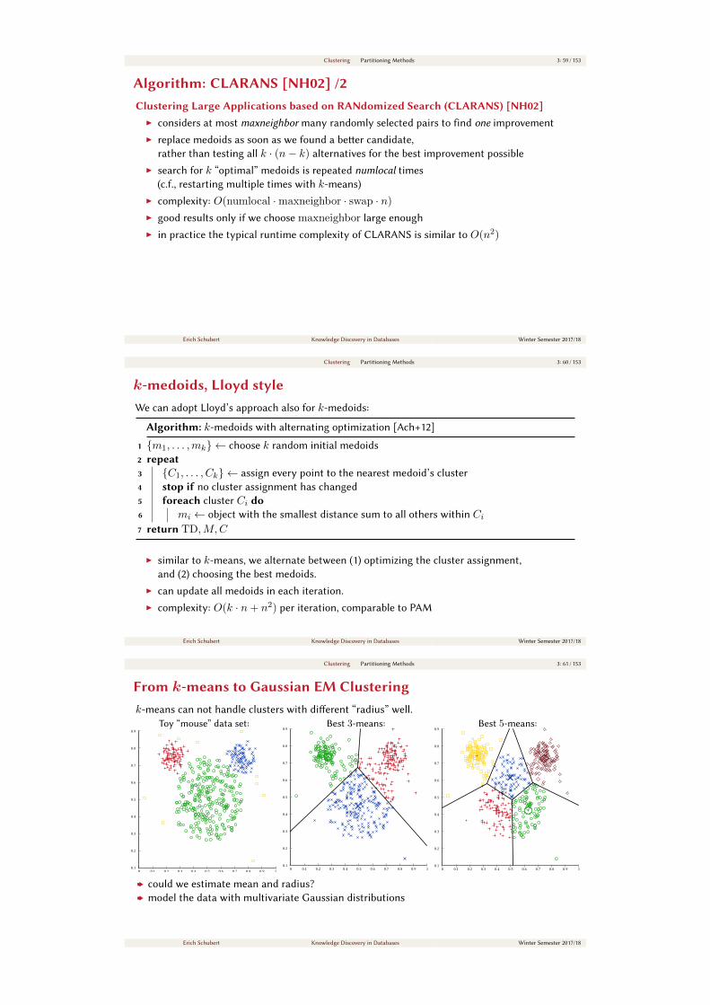
From k-means to Gaussian EM Clusteringk-means can not handle clusters with dierent “radius” well.
Toy “mouse” data set:
0 0.1 0.2 0.3 0.4 0.5 0.6 0.7 0.8 0.9 10.1
0.2
0.3
0.4
0.5
0.6
0.7
0.8
0.9
Best 3-means:
0 0.1 0.2 0.3 0.4 0.5 0.6 0.7 0.8 0.9 10.1
0.2
0.3
0.4
0.5
0.6
0.7
0.8
0.9Best 5-means:
0 0.1 0.2 0.3 0.4 0.5 0.6 0.7 0.8 0.9 10.1
0.2
0.3
0.4
0.5
0.6
0.7
0.8
0.9
z could we estimate mean and radius?
z model the data with multivariate Gaussian distributions
Erich Schubert Knowledge Discovery in Databases Winter Semester 2017/18

Clustering Model Optimization Methods 3: 62 / 153
Expectation-Maximization ClusteringEM (Expectation-Maximization) is the underlying principle in Lloyd’s k-means:
1. Choose initial model parameters θ
2. Expect latent variables (e.g., cluster assignment) from θ and the data.
3. Update θ to maximize the likelihood of observing the data
4. Repeat (2.)–(3.) until a stopping condition holds
Recall Lloyd’s k-means:
1. Choose k centers randomly (θ: random centers)
2. Expect cluster labels by choosing the nearest center as label
3. Update cluster centers with maximum-likelihood estimation of centrality
4. Repeat (2.)–(3.) until change = 0
Objective: optimize SSQ.
Erich Schubert Knowledge Discovery in Databases Winter Semester 2017/18
Clustering Model Optimization Methods 3: 62 / 153
Expectation-Maximization ClusteringEM (Expectation-Maximization) is the underlying principle in Lloyd’s k-means:
1. Choose initial model parameters θ
2. Expect latent variables (e.g., cluster assignment) from θ and the data.
3. Update θ to maximize the likelihood of observing the data
4. Repeat (2.)–(3.) until a stopping condition holds
Gaussian Mixture Modeling (GMM): [DLR77]
1. Choose k centers randomly, unit covariance, and uniform weight:
θ = (µ1,Σ1, w1, µ2,Σ2, w2, . . . µk,Σk, wk)
2. Expect cluster labels based on Gaussian distribution density
3. Update Gaussians with mean and covariance matrix
4. Repeat (2.)–(3.) until change < ε
Objective: Optimize log-likelihood: logL(θ) :=∑
x logP (x | θ)
Erich Schubert Knowledge Discovery in Databases Winter Semester 2017/18
Clustering Model Optimization Methods 3: 63 / 153
Gaussian Mixture Modeling & EMThe multivariate Gaussian density with center µi and covariance matrix Σi is:
P (x | Ci) =pdf(x, µi,Σi) := 1√(2π)d|Σi|
· e−12((x−µi)TΣ−1
i (x−µi))
For the Expectation Step, we use Bayes’ rule:
P (Ci | x) =pdf(x, µi,Σi)P (Ci)
P (x)
Using P (Ci) = wi and the law of total probability:
P (Ci | x) =wipdf(p, µi,Σi)∑
j wjpdf(p, µj ,Σj)
For the Maximization Step:
Use weighted mean and weighted covariance to recompute cluster model.
µi,j = 1∑x P (Ci | x)
∑xP (Ci | x)xj
Σi,j,k = 1∑x P (Ci | x)
∑xP (Ci | x)(xj − µj)(xk − µk)
wi =P (Ci) = 1|X|
∑xP (Ci | x)
P (Ci | x) is the relative
“responsibility” of Ci for point xP (Ci |x) proportional to wi ·pdfiP (Ci | x) ∝ wipdf(p, µi,Σi)
weighted X / SXYi cluster, j, k dimensions
weighted X / SXYi cluster, j, k dimensions
Erich Schubert Knowledge Discovery in Databases Winter Semester 2017/18
Clustering Model Optimization Methods 3: 64 / 153
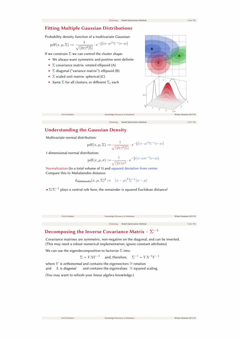
Fiing Multiple Gaussian Distributions
Probability density function of a multivariate Gaussian:
pdf(x, µ,Σ) :=1√
(2π)d|Σ|· e−
12((x−µ)TΣ−1(x−µ))
If we constrain Σ we can control the cluster shape:
I We always want symmetric and positive semi-definite
I Σ covariance matrix: rotated ellipsoid (A)
I Σ diagonal (“variance matrix”): ellipsoid (B)
I Σ scaled unit matrix: spherical (C)
I Same Σ for all clusters, or dierent Σi each
C
A
B
01
23
4 0
2
4
0
0.2
µ
Erich Schubert Knowledge Discovery in Databases Winter Semester 2017/18
Clustering Model Optimization Methods 3: 65 / 153
Understanding the Gaussian DensityMultivariate normal distribution:
pdf(x, µ,Σ) :=1√
(2π)d|Σ|· e−
12((x−µ)TΣ−1(x−µ))
1-dimensional normal distribution:
pdf(x, µ, σ) :=1√
(2π)σ2· e−
12((x−µ)σ−2(x−µ))
Normalization (to a total volume of 1) and squared deviation from center
Compare this to Mahalanobis distance:
dMahalanobis(x, µ,Σ)2 := (x− µ)TΣ−1(x− µ)
zΣ/Σ−1plays a central role here, the remainder is squared Euclidean distance!
Erich Schubert Knowledge Discovery in Databases Winter Semester 2017/18
Clustering Model Optimization Methods 3: 66 / 153
Decomposing the Inverse Covariance Matrix – Σ−1
Covariance matrixes are symmetric, non-negative on the diagonal, and can be inverted.
(This may need a robust numerical implementation; ignore constant aributes)
We can use the eigendecomposition to factorize Σ into:
Σ = V ΛV −1and, therefore, Σ−1 = V Λ−1V −1
where V is orthonormal and contains the eigenvectors∼= rotation
and Λ is diagonal and contains the eigenvalues∼= squared scaling.
(You may want to refresh your linear algebra knowledge.)
Erich Schubert Knowledge Discovery in Databases Winter Semester 2017/18
Clustering Model Optimization Methods 3: 67 / 153
Decomposing the Inverse Covariance Matrix – Σ−1 /2Based on this decomposition Σ = V ΛV −1
, let λi be the diagonal entries of Λ.
Build Ω using ωi =√λi−1
= λ− 1
2i . Then ΩT = Ω (because it is diagonal) and Λ−1 = ΩTΩ.
Σ−1 = V Λ−1V −1 = V ΩTΩV T = (ΩV T )TΩV T
d2Mahalanobis
= (x− µ)TΣ−1(x− µ)
= (x− µ)T (ΩV T )TΩV T (x− µ)
=⟨ΩV T (x− µ),ΩV T (x− µ)
⟩=∥∥ΩV T (x− µ)
∥∥2
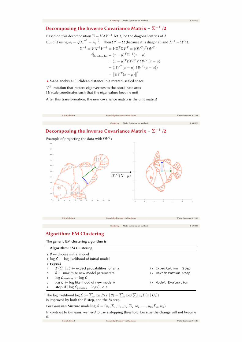
zMahalanobis ≈ Euclidean distance in a rotated, scaled space.
V T: rotation that rotates eigenvectors to the coordinate axes
Ω: scale coordinates such that the eigenvalues become unit
Aer this transformation, the new covariance matrix is the unit matrix!
Erich Schubert Knowledge Discovery in Databases Winter Semester 2017/18
Clustering Model Optimization Methods 3: 68 / 153
Decomposing the Inverse Covariance Matrix – Σ−1 /2Example of projecting the data with ΩV T
:
0 10 20 30 40 50 60 70 80 90 1000
10
20
30
40
50
60
70
80
90
100
-3 -2 -1 0 1 2 3-3
-2
-1
0
1
2
3
ΩV T(X−µ)
Erich Schubert Knowledge Discovery in Databases Winter Semester 2017/18
Clustering Model Optimization Methods 3: 69 / 153
Algorithm: EM ClusteringThe generic EM clustering algorithm is:
Algorithm: EM Clustering
1 θ ← choose initial model
2 logL ← log likelihood of initial model
3 repeat4 P (Ci | x)← expect probabilities for all x // Expectation Step5 θ ← maximize new model parameters // Maximization Step6 logLprevious ← logL7 logL ← log likelihood of new model θ // Model Evaluation8 stop if | logLprevious − logL| < ε
The log likelihood logL :=∑
x logP (x | θ) =∑
x log (∑
iwiP (x | Ci))is improved by both the E-step, and the M-step.
For Gaussian Mixture modeling, θ = (µ1,Σ1, w1, µ2,Σ2, w2, . . . , µk,Σk, wk)
In contrast to k-means, we need to use a stopping threshold, because the change will not become
0.
Erich Schubert Knowledge Discovery in Databases Winter Semester 2017/18
Clustering Model Optimization Methods 3: 70 / 153
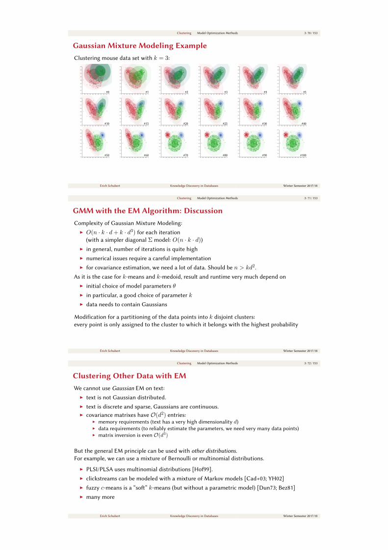
Gaussian Mixture Modeling ExampleClustering mouse data set with k = 3:
#00 0.1 0.2 0.3 0.4 0.5 0.6 0.7 0.8 0.9 10.1
0.2
0.3
0.4
0.5
0.6
0.7
0.8
0.9
#10 0.1 0.2 0.3 0.4 0.5 0.6 0.7 0.8 0.9 10.1
0.2
0.3
0.4
0.5
0.6
0.7
0.8
0.9
#20 0.1 0.2 0.3 0.4 0.5 0.6 0.7 0.8 0.9 10.1
0.2
0.3
0.4
0.5
0.6
0.7
0.8
0.9
#30 0.1 0.2 0.3 0.4 0.5 0.6 0.7 0.8 0.9 10.1
0.2
0.3
0.4
0.5
0.6
0.7
0.8
0.9
#40 0.1 0.2 0.3 0.4 0.5 0.6 0.7 0.8 0.9 10.1
0.2
0.3
0.4
0.5
0.6
0.7
0.8
0.9
#50 0.1 0.2 0.3 0.4 0.5 0.6 0.7 0.8 0.9 10.1
0.2
0.3
0.4
0.5
0.6
0.7
0.8
0.9
#100 0.1 0.2 0.3 0.4 0.5 0.6 0.7 0.8 0.9 10.1
0.2
0.3
0.4
0.5
0.6
0.7
0.8
0.9
#150 0.1 0.2 0.3 0.4 0.5 0.6 0.7 0.8 0.9 10.1
0.2
0.3
0.4
0.5
0.6
0.7
0.8
0.9
#200 0.1 0.2 0.3 0.4 0.5 0.6 0.7 0.8 0.9 10.1
0.2
0.3
0.4
0.5
0.6
0.7
0.8
0.9
#250 0.1 0.2 0.3 0.4 0.5 0.6 0.7 0.8 0.9 10.1
0.2
0.3
0.4
0.5
0.6
0.7
0.8
0.9
#300 0.1 0.2 0.3 0.4 0.5 0.6 0.7 0.8 0.9 10.1
0.2
0.3
0.4
0.5
0.6
0.7
0.8
0.9
#400 0.1 0.2 0.3 0.4 0.5 0.6 0.7 0.8 0.9 10.1
0.2
0.3
0.4
0.5
0.6
0.7
0.8
0.9
#500 0.1 0.2 0.3 0.4 0.5 0.6 0.7 0.8 0.9 10.1
0.2
0.3
0.4
0.5
0.6
0.7
0.8
0.9
#600 0.1 0.2 0.3 0.4 0.5 0.6 0.7 0.8 0.9 10.1
0.2
0.3
0.4
0.5
0.6
0.7
0.8
0.9
#700 0.1 0.2 0.3 0.4 0.5 0.6 0.7 0.8 0.9 10.1
0.2
0.3
0.4
0.5
0.6
0.7
0.8
0.9
#800 0.1 0.2 0.3 0.4 0.5 0.6 0.7 0.8 0.9 10.1
0.2
0.3
0.4
0.5
0.6
0.7
0.8
0.9
#900 0.1 0.2 0.3 0.4 0.5 0.6 0.7 0.8 0.9 10.1
0.2
0.3
0.4
0.5
0.6
0.7
0.8
0.9
#1000 0.1 0.2 0.3 0.4 0.5 0.6 0.7 0.8 0.9 10.1
0.2
0.3
0.4
0.5
0.6
0.7
0.8
0.9
Erich Schubert Knowledge Discovery in Databases Winter Semester 2017/18
Clustering Model Optimization Methods 3: 71 / 153
GMM with the EM Algorithm: DiscussionComplexity of Gaussian Mixture Modeling:
I O(n · k · d+ k · d3) for each iteration
(with a simpler diagonal Σ model: O(n · k · d))
I in general, number of iterations is quite high
I numerical issues require a careful implementation
I for covariance estimation, we need a lot of data. Should be n > kd2.
As it is the case for k-means and k-medoid, result and runtime very much depend on
I initial choice of model parameters θ
I in particular, a good choice of parameter k
I data needs to contain Gaussians
Modification for a partitioning of the data points into k disjoint clusters:
every point is only assigned to the cluster to which it belongs with the highest probability
Erich Schubert Knowledge Discovery in Databases Winter Semester 2017/18
Clustering Model Optimization Methods 3: 72 / 153
Clustering Other Data with EMWe cannot use Gaussian EM on text:
I text is not Gaussian distributed.
I text is discrete and sparse, Gaussians are continuous.
I covariance matrixes have O(d2) entries:
I memory requirements (text has a very high dimensionality d)
I data requirements (to reliably estimate the parameters, we need very many data points)
I matrix inversion is even O(d3)
But the general EM principle can be used with other distributions.For example, we can use a mixture of Bernoulli or multinomial distributions.
I PLSI/PLSA uses multinomial distributions [Hof99].
I clickstreams can be modeled with a mixture of Markov models [Cad+03; YH02]
I fuzzy c-means is a “so” k-means (but without a parametric model) [Dun73; Bez81]
I many more
Erich Schubert Knowledge Discovery in Databases Winter Semester 2017/18
Clustering Model Optimization Methods 3: 73 / 153
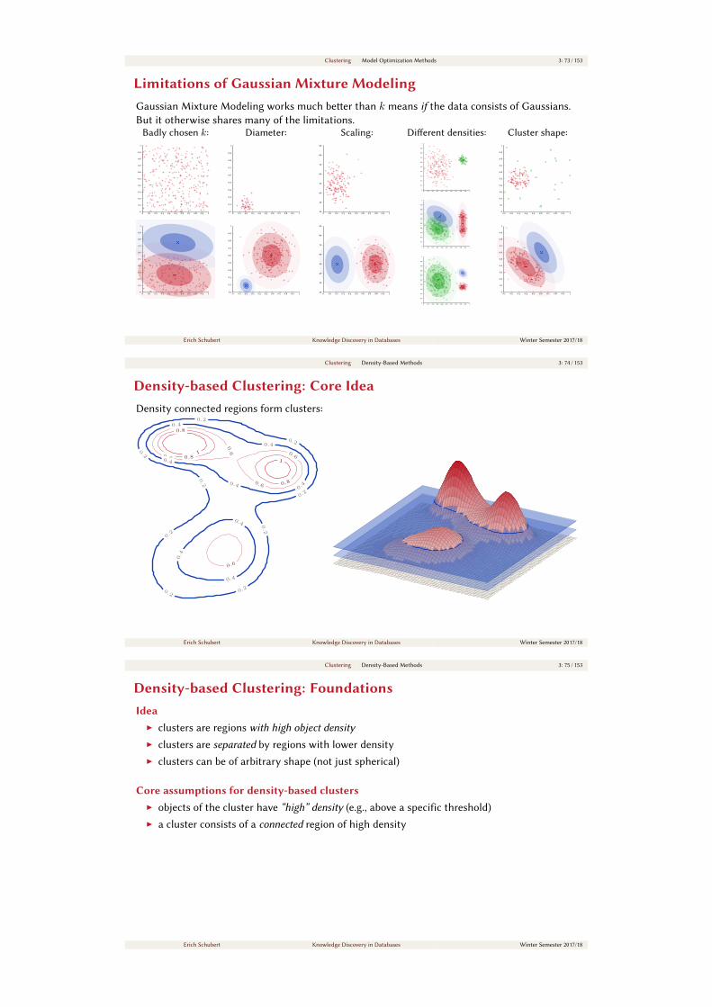
Limitations of Gaussian Mixture ModelingGaussian Mixture Modeling works much beer than k means if the data consists of Gaussians.
But it otherwise shares many of the limitations.
Badly chosen k:
0 0.1 0.2 0.3 0.4 0.5 0.6 0.7 0.8 0.9 10
0.1
0.2
0.3
0.4
0.5
0.6
0.7
0.8
0.9
1
0 0.1 0.2 0.3 0.4 0.5 0.6 0.7 0.8 0.9 10
0.1
0.2
0.3
0.4
0.5
0.6
0.7
0.8
0.9
1
Diameter:
0 0.1 0.2 0.3 0.4 0.5 0.6 0.7 0.8 0.9 10.1
0.2
0.3
0.4
0.5
0.6
0.7
0.8
0.9
1
0 0.1 0.2 0.3 0.4 0.5 0.6 0.7 0.8 0.9 10.1
0.2
0.3
0.4
0.5
0.6
0.7
0.8
0.9
1
Scaling:
0 0.1 0.2 0.3 0.4 0.5 0.6 0.7 0.8 0.9 120
30
40
50
60
70
80
90
0 0.1 0.2 0.3 0.4 0.5 0.6 0.7 0.8 0.9 120
30
40
50
60
70
80
90
Dierent densities:
0 0.1 0.2 0.3 0.4 0.5 0.6 0.7 0.8 0.9 10
0.1
0.2
0.3
0.4
0.5
0.6
0.7
0.8
0.9
1
0 0.1 0.2 0.3 0.4 0.5 0.6 0.7 0.8 0.9 10
0.1
0.2
0.3
0.4
0.5
0.6
0.7
0.8
0.9
1
0 0.1 0.2 0.3 0.4 0.5 0.6 0.7 0.8 0.9 10
0.1
0.2
0.3
0.4
0.5
0.6
0.7
0.8
0.9
1
Cluster shape:
0.1 0.2 0.3 0.4 0.5 0.6 0.7 0.8 0.9 10
0.1
0.2
0.3
0.4
0.5
0.6
0.7
0.8
0.9
1
0.1 0.2 0.3 0.4 0.5 0.6 0.7 0.8 0.9 10
0.1
0.2
0.3
0.4
0.5
0.6
0.7
0.8
0.9
1
Erich Schubert Knowledge Discovery in Databases Winter Semester 2017/18
Clustering Density-Based Methods 3: 74 / 153
Density-based Clustering: Core IdeaDensity connected regions form clusters:
1
1
0.8
0.8
0.8
0.6
0.6
0.60.6
0.6
0.4
0.4
0.4
0.4
0.4
0.40.4
0.4
0.2
0.2
0.2
0.2
0.2
0.2
0.2
0.2
0.2
0.4
0.4
0.4
0.4
0.4
0.40.4
0.4
0.2
0.2
0.2
0.2
0.2
0.2
0.2
0.2
0.2
Erich Schubert Knowledge Discovery in Databases Winter Semester 2017/18
Clustering Density-Based Methods 3: 75 / 153
Density-based Clustering: FoundationsIdea
I clusters are regions with high object densityI clusters are separated by regions with lower density
I clusters can be of arbitrary shape (not just spherical)
Core assumptions for density-based clustersI objects of the cluster have “high” density (e.g., above a specific threshold)
I a cluster consists of a connected region of high density
Erich Schubert Knowledge Discovery in Databases Winter Semester 2017/18
Clustering Density-Based Methods 3: 76 / 153
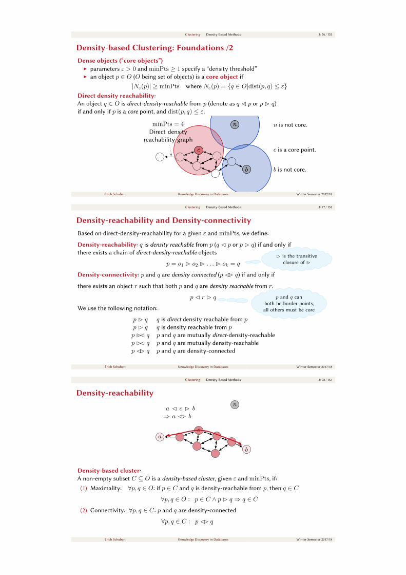
Density-based Clustering: Foundations /2Dense objects (“core objects”)
I parameters ε > 0 and minPts ≥ 1 specify a “density threshold”
I an object p ∈ O (O being set of objects) is a core object if
|Nε(p)| ≥ minPts where Nε(p) = q ∈ O|dist(p, q) ≤ εDirect density reachability:
An object q ∈ O is direct-density-reachable from p (denote as q ·C p or p ·B q)
if and only if p is a core point, and dist(p, q) ≤ ε.
minPts = 4
c
b
nn n is not core.
c c is a core point.
b b is not core.
Direct density
reachability graph
Erich Schubert Knowledge Discovery in Databases Winter Semester 2017/18
Clustering Density-Based Methods 3: 77 / 153
Density-reachability and Density-connectivityBased on direct-density-reachability for a given ε and minPts, we define:
Density-reachability: q is density reachable from p (q C p or p B q) if and only if
there exists a chain of direct-density-reachable objects
p = o1 ·B o2 ·B . . . ·B ok = qB is the transitive
closure of ·B
Density-connectivity: p and q are density connected (p CB q) if and only if
there exists an object r such that both p and q are density reachable from r.
p C r B q p and q can
both be border points,
all others must be coreWe use the following notation:
p ·B q q is direct density reachable from pp B q q is density reachable from pp ·B ·C q p and q are mutually direct-density-reachable
p BC q p and q are mutually density-reachable
p CB q p and q are density-connected
Erich Schubert Knowledge Discovery in Databases Winter Semester 2017/18
Clustering Density-Based Methods 3: 78 / 153
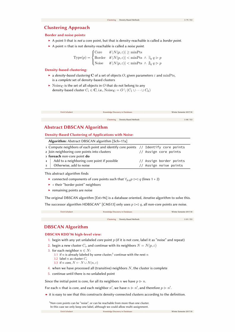
Density-reachability
c
b
n
a
a C c B b⇒ a CB b
Density-based cluster:
A non-empty subset C ⊆ O is a density-based cluster, given ε and minPts, if:
(1) Maximality: ∀p, q ∈ O: if p ∈ C and q is density-reachable from p, then q ∈ C
∀p, q ∈ O : p ∈ C ∧ p B q ⇒ q ∈ C
(2) Connectivity: ∀p, q ∈ C : p and q are density-connected
∀p, q ∈ C : p CB q
Erich Schubert Knowledge Discovery in Databases Winter Semester 2017/18
Clustering Density-Based Methods 3: 79 / 153
Clustering ApproachBorder and noise points:
I A point b that is not a core point, but that is density-reachable is called a border point.I A point n that is not density-reachable is called a noise point.
Type(p) =
Core if |N(p, ε)| ≥ minPts
Border if |N(p, ε)| < minPts ∧ ∃q q B p
Noise if |N(p, ε)| < minPts ∧ @q q B p
Density-based clustering:
I a density-based clustering C of a set of objects O, given parameters ε and minPts,
is a complete set of density-based clusters
I NoiseC is the set of all objects in O that do not belong to any
density-based cluster Ci ∈ C, i.e., NoiseC = O \ (C1 ∪ · · · ∪ Ck)
Erich Schubert Knowledge Discovery in Databases Winter Semester 2017/18
Clustering Density-Based Methods 3: 80 / 153
Abstract DBSCAN AlgorithmDensity-Based Clustering of Applications with Noise:
Algorithm: Abstract DBSCAN algorithm [Sch+17a]
1 Compute neighbors of each point and identify core points // Identify core points2 Join neighboring core points into clusters // Assign core points3 foreach non-core point do4 Add to a neighboring core point if possible // Assign border points5 Otherwise, add to noise // Assign noise points
This abstract algorithm finds
I connected components of core points such that ∀p,qp BC q (lines 1 + 2)
I + their “border point” neighbors
I remaining points are noise
The original DBSCAN algorithm [Est+96] is a database oriented, iterative algorithm to solve this.
The successor algorithm HDBSCAN* [CMS13] only uses p BC q, all non-core points are noise.
Erich Schubert Knowledge Discovery in Databases Winter Semester 2017/18
Clustering Density-Based Methods 3: 81 / 153
DBSCAN AlgorithmDBSCAN KDD’96 high-level view:
1. begin with any yet unlabeled core point p (if it is not core, label it as “noise” and repeat)
2. begin a new cluster Ci, and continue with its neighbors N = N(p, ε)
3. for each neighbor n ∈ N :
3.1 if n is already labeled by some cluster,5
continue with the next n3.2 label n as cluster Ci
3.3 if n core, N ← N ∪N(n, ε)
4. when we have processed all (transitive) neighbors N , the cluster is complete
5. continue until there is no unlabeled point
Since the initial point is core, for all its neighbors n we have p ·B n.
For each n that is core, and each neighbor n′, we have n ·B n′, and therefore p B n′.
z it is easy to see that this constructs density-connected clusters according to the definition.
5
Non-core points can be “noise”, or can be reachable from more than one cluster.
In this case we only keep one label, although we could allow multi-assignment.
Erich Schubert Knowledge Discovery in Databases Winter Semester 2017/18
Clustering Density-Based Methods 3: 82 / 153
DBSCAN Algorithm /2
Algorithm: Pseudocode of original sequential DBSCAN algorithm [Est+96; Sch+17a]
Data: label: Point labels, initially undefined1 foreach point p in database DB do // Iterate over every point2 if label(p) 6= undefined then continue // Skip processed points3 Neighbors N ← RangeQuery(DB,dist, p, ε) // Find initial neighbors4 if |N | < minPts then // Non-core points are noise5 label(p)← Noise6 continue7 c← next cluster label // Start a new cluster8 label(p)← c
9 Seed set S ← N \ p // Expand neighborhood10 foreach q in S do11 if label(q) = Noise then label(q)← c12 if label(q) 6= undefined then continue13 Neighbors N ← RangeQuery(DB,dist, q, ε)14 label(q)← c15 if |N | < minPts then continue // Core-point check16 S ← S ∪N
Erich Schubert Knowledge Discovery in Databases Winter Semester 2017/18
Clustering Density-Based Methods 3: 83 / 153
DBSCAN Algorithm /3Properties of the algorithm
I on core points and noise points, the result is exactly according to the definitions
I border points are only in one cluster, from which they are reachable
(This could trivially be allowed, but is not desirable in practise!)
I complexity: O(n · T ) with T the complexity to find the ε-neighbors
In many applications T ≈ log n with indexing, but this cannot be guaranteed.
Typical indexed behavior then is n log n, but worst-case is O(n2) distance computations.
ChallengesI how to choose ε and minPts?
I which distance function to use?
I which index for acceleration?
I how to evaluate the result?
Erich Schubert Knowledge Discovery in Databases Winter Semester 2017/18
Clustering Density-Based Methods 3: 84 / 153
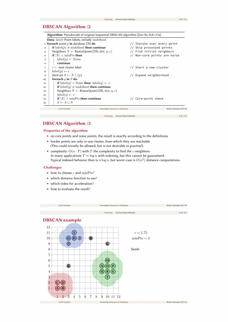
DBSCAN example
1 2 3 4 5 6 7 8 9 10 11 12
1
2
3
4
5
6
7
8
9
10
11
12
A B
C D
A
C
B
D
EE
F
G H
IJ
F
G
F
H J
I
K
L
K
L
M
N O P
Q R S
T
M
O
R
T
Q
N P
S
ε = 1.75
minPts = 4
Seeds
Erich Schubert Knowledge Discovery in Databases Winter Semester 2017/18
Clustering Density-Based Methods 3: 85 / 153
Choosing DBSCAN parametersChoosing minPts:
I usually easier to choose
I heuristic: 2×dimensionality [Est+96]
I choose larger values for large and noisy data sets [Sch+17a]
Choosing ε:
I too large clusters: reduce radius ε [Sch+17a]
I too much noise: increase radius ε [Sch+17a]
I first guess: based on distances to the (minPts− 1)-nearest neighbor [Est+96]
Detecting bad parameters: [Sch+17a]
I ε range query results are too large⇒ slow execution
I almost all points are in the same cluster (largest cluster should be < 20% to < 50% usually)
I too much noise (should usually be 1% to < 30%, depending on the application)
Erich Schubert Knowledge Discovery in Databases Winter Semester 2017/18
Clustering Density-Based Methods 3: 86 / 153
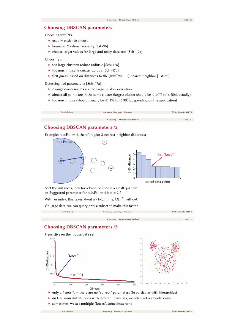
Choosing DBSCAN parameters /2Example: minPts = 4, therefore plot 3-nearest-neighbor distances:
minPts = 4
c
b
n
a
0
1
2
3
4
5
3N
Nd
istan
ce
sorted data points
first “knee”
Sort the distances, look for a knee, or choose a small quantile.
⇒ Suggested parameter for minPts = 4 is ε ≈ 2.5
With an index, this takes about n · log n time, O(n2) without.
On large data, we can query only a subset to make this faster.
Erich Schubert Knowledge Discovery in Databases Winter Semester 2017/18
Clustering Density-Based Methods 3: 87 / 153
Choosing DBSCAN parameters /3Heuristics on the mouse data set.
0
0.05
0.1
0.15
0.2
0.25
0 100 200 300 400 500
Objects
2-NN-distance
“Knee”?
ε = 0.04
0 0.1 0.2 0.3 0.4 0.5 0.6 0.7 0.8 0.9 10.1
0.2
0.3
0.4
0.5
0.6
0.7
0.8
0.9
I only a heuristic — there are no “correct” parameters (in particular with hierarchies)
I on Gaussian distributions with dierent densities, we oen get a smooth curve
I sometimes, we see multiple “knees”, sometimes none
Erich Schubert Knowledge Discovery in Databases Winter Semester 2017/18
Clustering Density-Based Methods 3: 87 / 153
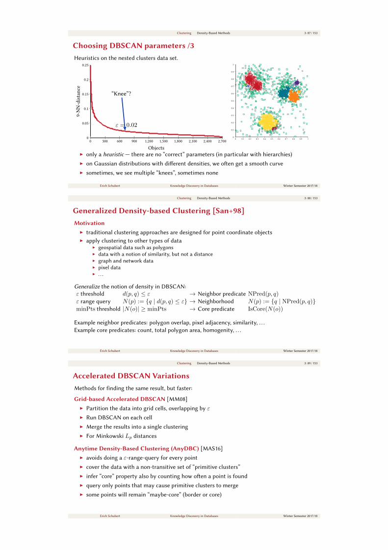
Choosing DBSCAN parameters /3Heuristics on the nested clusters data set.
0
0.05
0.1
0.15
0.2
0.25
0 300 600 900 1,200 1,500 1,800 2,100 2,400 2,700
Objects
9-NN-distance
“Knee”?
ε = 0.02
0 0.1 0.2 0.3 0.4 0.5 0.6 0.7 0.8 0.9 10
0.1
0.2
0.3
0.4
0.5
0.6
0.7
0.8
0.9
1
I only a heuristic — there are no “correct” parameters (in particular with hierarchies)
I on Gaussian distributions with dierent densities, we oen get a smooth curve
I sometimes, we see multiple “knees”, sometimes none
Erich Schubert Knowledge Discovery in Databases Winter Semester 2017/18
Clustering Density-Based Methods 3: 88 / 153
Generalized Density-based Clustering [San+98]Motivation
I traditional clustering approaches are designed for point coordinate objects
I apply clustering to other types of data
I geospatial data such as polygons
I data with a notion of similarity, but not a distance
I graph and network data
I pixel data
I . . .
Generalize the notion of density in DBSCAN:
ε threshold d(p, q) ≤ ε → Neighbor predicate NPred(p, q)ε range query N(p) := q | d(p, q) ≤ ε → Neighborhood N(p) := q | NPred(p, q)minPts threshold |N(o)| ≥ minPts → Core predicate IsCore(N(o))
Example neighbor predicates: polygon overlap, pixel adjacency, similarity, . . .
Example core predicates: count, total polygon area, homogenity, . . .
Erich Schubert Knowledge Discovery in Databases Winter Semester 2017/18
Clustering Density-Based Methods 3: 89 / 153
Accelerated DBSCAN VariationsMethods for finding the same result, but faster:
Grid-based Accelerated DBSCAN [MM08]
I Partition the data into grid cells, overlapping by ε
I Run DBSCAN on each cell
I Merge the results into a single clustering
I For Minkowski Lp distances
Anytime Density-Based Clustering (AnyDBC) [MAS16]
I avoids doing a ε-range-query for every point
I cover the data with a non-transitive set of “primitive clusters”
I infer “core” property also by counting how oen a point is found
I query only points that may cause primitive clusters to merge
I some points will remain “maybe-core” (border or core)
Erich Schubert Knowledge Discovery in Databases Winter Semester 2017/18
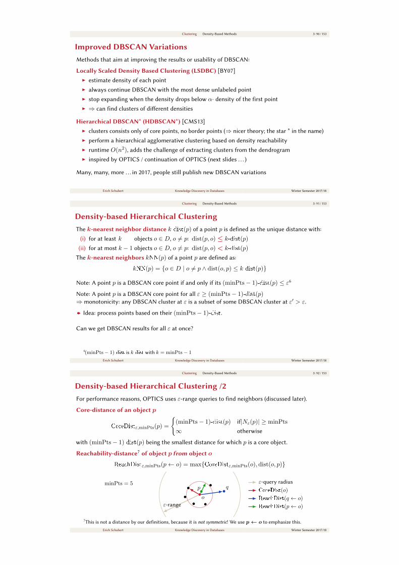
Clustering Density-Based Methods 3: 90 / 153
Improved DBSCAN VariationsMethods that aim at improving the results or usability of DBSCAN:
Locally Scaled Density Based Clustering (LSDBC) [BY07]
I estimate density of each point
I always continue DBSCAN with the most dense unlabeled point
I stop expanding when the density drops below α· density of the first point
I ⇒ can find clusters of dierent densities
Hierarchical DBSCAN* (HDBSCAN*) [CMS13]
I clusters consists only of core points, no border points (⇒ nicer theory; the star * in the name)
I perform a hierarchical agglomerative clustering based on density reachability
I runtime O(n2), adds the challenge of extracting clusters from the dendrogram
I inspired by OPTICS / continuation of OPTICS (next slides . . . )
Many, many, more . . . in 2017, people still publish new DBSCAN variations
Erich Schubert Knowledge Discovery in Databases Winter Semester 2017/18
Clustering Density-Based Methods 3: 91 / 153
Density-based Hierarchical ClusteringThe k-nearest neighbor distance k-dist(p) of a point p is defined as the unique distance with:
(i) for at least k objects o ∈ D, o 6= p: dist(p, o) ≤ k-dist(p)
(ii) for at most k − 1 objects o ∈ D, o 6= p: dist(p, o) < k-dist(p)
The k-nearest neighbors kNN(p) of a point p are defined as:
kNN(p) = o ∈ D | o 6= p ∧ dist(o, p) ≤ k-dist(p)
Note: A point p is a DBSCAN core point if and only if its (minPts− 1)-dist(p) ≤ ε6
Note: A point p is a DBSCAN core point for all ε ≥ (minPts− 1)-dist(p)⇒ monotonicity: any DBSCAN cluster at ε is a subset of some DBSCAN cluster at ε′ > ε.
z Idea: process points based on their (minPts− 1)-dist.
Can we get DBSCAN results for all ε at once?
6(minPts− 1)-dist is k-dist with k = minPts− 1
Erich Schubert Knowledge Discovery in Databases Winter Semester 2017/18
Clustering Density-Based Methods 3: 92 / 153
Density-based Hierarchical Clustering /2For performance reasons, OPTICS uses ε-range queries to find neighbors (discussed later).
Core-distance of an object p
CoreDistε,minPts(p) =
(minPts− 1)-dist(p) if|Nε(p)| ≥ minPts
∞ otherwise
with (minPts− 1)-dist(p) being the smallest distance for which p is a core object.
Reachability-distance7 of object p from object o
ReachDistε,minPts(p← o) = maxCoreDistε,minPts(o), dist(o, p)
ε-range
minPts = 5
o
qpε-query radius
CoreDist(o)
ReachDist(q ← o)
ReachDist(p← o)
7
This is not a distance by our definitions, because it is not symmetric! We use p← o to emphasize this.
Erich Schubert Knowledge Discovery in Databases Winter Semester 2017/18
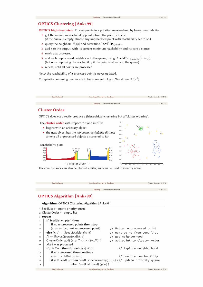
Clustering Density-Based Methods 3: 93 / 153
OPTICS Clustering [Ank+99]OPTICS high-level view: Process points in a priority queue ordered by lowest reachability.
1. get the minimum-reachability point p from the priority queue
(if the queue is empty, choose any unprocessed point with reachability set to∞.)
2. query the neighbors Nε(p) and determine CoreDistε,minPts
3. add p to the output, with its current minimum reachability and its core distance
4. mark p as processed
5. add each unprocessed neighbor n to the queue, using ReachDistε,minPts(n← p),
(but only improving the reachability if the point is already in the queue)
6. repeat, until all points are processed
Note: the reachability of a processed point is never updated.
Complexity: assuming queries are in log n, we get n log n. Worst case: O(n2)
Erich Schubert Knowledge Discovery in Databases Winter Semester 2017/18
Clustering Density-Based Methods 3: 94 / 153
Cluster OrderOPTICS does not directly produce a (hierarchical) clustering but a “cluster ordering”.
The cluster order with respect to ε and minPts
I begins with an arbitrary object
I the next object has the minimum reachability distanceamong all unprocessed objects discovered so far
Reachability plot:
0.060.110.160.210.260.31
0.060.110.160.210.260.31A B C D E F G H
→ cluster order→ 0 0.1 0.2 0.3 0.4 0.5 0.6 0.7 0.8 0.9 10
0.1
0.2
0.3
0.4
0.5
0.6
0.7
0.8
0.9
1
A
B
C
DE
F
G
H
The core distance can also be ploed similar, and can be used to identify noise.
Erich Schubert Knowledge Discovery in Databases Winter Semester 2017/18
Clustering Density-Based Methods 3: 95 / 153
OPTICS Algorithm [Ank+99]
Algorithm: OPTICS Clustering Algorithm [Ank+99]
1 SeedList← empty priority queue
2 ClusterOrder← empty list
3 repeat4 if SeedList.empty() then5 if no unprocessed points then stop6 (r, o)← (∞, next unprocessed point) // Get an unprocessed point7 else (r, o)← SeedList.deleteMin() // next point from seed list8 N ← RangeQuery(o, dist, ε) // get neighborhood9 ClusterOrder.add( (r, o,CoreDist(o,N)) ) // add point to cluster order
10 Mark o as processed
11 if p is Core then foreach n ∈ N do // Explore neighborhood12 if n is processed then continue13 p← ReachDist(n← o) // compute reachability14 if n ∈ SeedList then SeedList.decreaseKey( (p, n) ) // update priority queue15 else SeedList.insert( (p, n) )
Erich Schubert Knowledge Discovery in Databases Winter Semester 2017/18
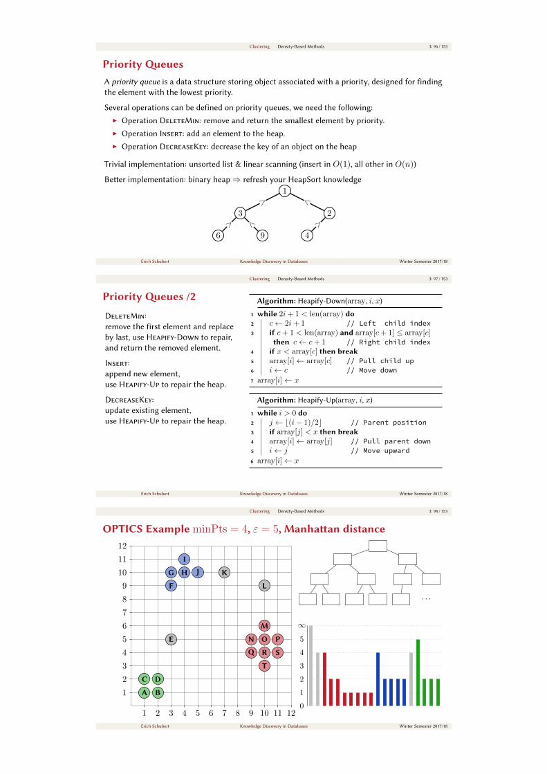
Clustering Density-Based Methods 3: 96 / 153
Priority euesA priority queue is a data structure storing object associated with a priority, designed for finding
the element with the lowest priority.
Several operations can be defined on priority queues, we need the following:
I Operation DeleteMin: remove and return the smallest element by priority.
I Operation Insert: add an element to the heap.
I Operation DecreaseKey: decrease the key of an object on the heap
Trivial implementation: unsorted list & linear scanning (insert in O(1), all other in O(n))
Beer implementation: binary heap⇒ refresh your HeapSort knowledge
1
3
6>
9
<
>2
4>
<
Erich Schubert Knowledge Discovery in Databases Winter Semester 2017/18
Clustering Density-Based Methods 3: 97 / 153
Priority eues /2
DeleteMin:
remove the first element and replace
by last, use Heapify-Down to repair,
and return the removed element.
Insert:
append new element,
use Heapify-Up to repair the heap.
DecreaseKey:
update existing element,
use Heapify-Up to repair the heap.
Algorithm: Heapify-Down(array, i, x)
1 while 2i+ 1 < len(array) do2 c← 2i+ 1 // Left child index3 if c+ 1 < len(array) and array[c+ 1] ≤ array[c]
then c← c+ 1 // Right child index4 if x < array[c] then break5 array[i]← array[c] // Pull child up6 i← c // Move down7 array[i]← x
Algorithm: Heapify-Up(array, i, x)
1 while i > 0 do2 j ← b(i− 1)/2c // Parent position3 if array[j] < x then break4 array[i]← array[j] // Pull parent down5 i← j // Move upward6 array[i]← x
Erich Schubert Knowledge Discovery in Databases Winter Semester 2017/18
Clustering Density-Based Methods 3: 98 / 153
OPTICS Example minPts = 4, ε = 5, Manhaan distance
1 2 3 4 5 6 7 8 9 10 11 12
1
2
3
4
5
6
7
8
9
10
11
12
A B
C D
E
F
G H
IJ K
L
M
N O P
Q R S
T
· · ·
0
1
2
3
4
5
∞
A B
C D
E
F
G H
IJ K
L
M
N O P
Q R S
T
Erich Schubert Knowledge Discovery in Databases Winter Semester 2017/18
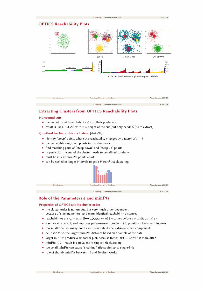
Clustering Density-Based Methods 3: 99 / 153
OPTICS Reachability Plots
0 0.1 0.2 0.3 0.4 0.5 0.6 0.7 0.8 0.9 10.1
0.2
0.3
0.4
0.5
0.6
0.7
0.8
0.9
0.02
0.13
0.24
0.02
0.13
0.24
right ear le ear
0 0.1 0.2 0.3 0.4 0.5 0.6 0.7 0.8 0.9 10
0.1
0.2
0.3
0.4
0.5
0.6
0.7
0.8
0.9
1
0 0.1 0.2 0.3 0.4 0.5 0.6 0.7 0.8 0.9 10
0.1
0.2
0.3
0.4
0.5
0.6
0.7
0.8
0.9
1
0 0.1 0.2 0.3 0.4 0.5 0.6 0.7 0.8 0.9 10
0.1
0.2
0.3
0.4
0.5
0.6
0.7
0.8
0.9
1
Labels Cut at 0.019 Cut at 0.08
00.040.080.120.160.2
00.040.080.120.160.2
Colors in the cluster order plot correspond to labels!
Erich Schubert Knowledge Discovery in Databases Winter Semester 2017/18
Clustering Density-Based Methods 3: 100 / 153
Extracting Clusters from OPTICS Reachability PlotsHorizontal cut:
I merge points with reachability ≤ ε to their predecessor
I result is like DBSCAN with ε = height of the cut (but only needs O(n) to extract)
ξ method for hierarchical clusters: [Ank+99]
I identify “steep” points where the reachability changes by a factor of 1− ξI merge neighboring steep points into a steep area.
I find matching pairs of “steep down” and “steep up” points
I in particular the end of the cluster needs to be refined carefully
I must be at least minPts points apart
I can be nested in longer intervals to get a hierarchical clustering
Erich Schubert Knowledge Discovery in Databases Winter Semester 2017/18
Clustering Density-Based Methods 3: 101 / 153
Role of the Parameters ε and minPts
Properties of OPTICS and its cluster orderI the cluster order is not unique, but very much order dependent
because of starting point(s) and many identical reachability distances
I reachabilities are rp = minReachDist(p← n) | n comes before p ∧ dist(p, n) ≤ ε.I ε serves as a cut-o, and improves performance from O(n2) to possibly n log n with indexes
I too small ε causes many points with reachability∞ = disconnected components
I heuristic for ε: the largest minPts-distance based on a sample of the data
I larger minPts produce a smoother plot, because ReachDist = CoreDist more oen
I minPts ≤ 2 – result is equivalent to single-link clustering
I too small minPts can cause “chaining” eects similar to single-link
I rule of thumb: minPts between 10 and 50 oen works
Erich Schubert Knowledge Discovery in Databases Winter Semester 2017/18

Clustering Density-Based Methods 3: 102 / 153
Other Density-based Clustering AlgorithmsMean-Shi: [FH75]
I Replace each point with the weighted average of its ε neighbors.
I Points that move to the same location (± a small threshold) form a cluster
I Runtime: O(n2) per iteration, many iterations
DenClue: [HK98]
I Use kernel density estimation
I Use gradients to find density maxima
I Approximate the data using a grid [HG07]
Density-Peak Clustering: [RL14]
I Estimate density of each point
I Every point connects to the nearest neighbor of higher density
I Runtime: O(n2); needs user input to select clusters
Erich Schubert Knowledge Discovery in Databases Winter Semester 2017/18
Clustering Biclustering Methods 3: 103 / 153
Biclustering & Subspace ClusteringPopular in gene expression analysis.
I Every row is a gene
I Every column is a sample
or transposed
I Only a few genes are relevant
I No semantic ordering of rows or columns
I Some samples may be contaminated
I Numerical value may be unreliable, only “high” or “low”
z Key idea of biclustering: Cheng and Church [CC00]
Find a subset of rows and columns (submatrix, aer permutation),
such that all values are high/low or exhibit some paern.
Erich Schubert Knowledge Discovery in Databases Winter Semester 2017/18
Clustering Biclustering Methods 3: 104 / 153
Bicluster Paerns [CC00]Some examples for bicluster paerns:
1
1
1
1
1
1
1
1
1
1
1
1
1
1
1
1
1
1
1
1
1
1
1
1
1
1
1
1
1
1
1
1
1
1
1
1
constant
1
1
1
1
1
1
2
2
2
2
2
2
3
3
3
3
3
3
4
4
4
4
4
4
5
5
5
5
5
5
6
6
6
6
6
6
rows
6
5
4
3
2
1
6
5
4
3
2
1
6
5
4
3
2
1
6
5
4
3
2
1
6
5
4
3
2
1
6
5
4
3
2
1
columns
6
5
4
3
2
1
7
6
5
4
3
2
8
7
6
5
4
3
9
8
7
6
5
4
10
9
8
7
6
5
11
10
9
8
7
6
additive
1
3
2
4
1.5
0.5
2
6
4
8
3
1
4
12
8
16
6
2
0
0
0
0
0
0
4
12
8
16
6
2
3
9
6
12
4.5
1.5
multiplicative
I clusters may overlap in rows and columns
I paerns will never be this ideal, but noisy!
I many algorithms focus on the constant paern type only, as there are O(2N ·d) possibilities.
Erich Schubert Knowledge Discovery in Databases Winter Semester 2017/18
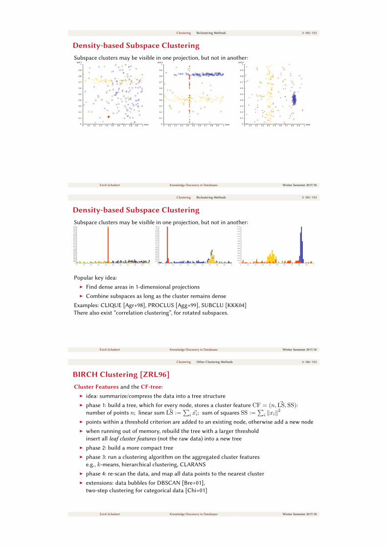
Clustering Biclustering Methods 3: 105 / 153
Density-based Subspace ClusteringSubspace clusters may be visible in one projection, but not in another:
0 0.1 0.2 0.3 0.4 0.5 0.6 0.7 0.8 0.9 1 Column 00
0.1
0.2
0.3
0.4
0.5
0.6
0.7
0.8
0.9
1Column 1
0 0.1 0.2 0.3 0.4 0.5 0.6 0.7 0.8 0.9 1 Column 00
0.1
0.2
0.3
0.4
0.5
0.6
0.7
0.8
0.9
1Column 2
0 0.1 0.2 0.3 0.4 0.5 0.6 0.7 0.8 0.9 1 Column 20
0.1
0.2
0.3
0.4
0.5
0.6
0.7
0.8
0.9
1Column 3
Erich Schubert Knowledge Discovery in Databases Winter Semester 2017/18
Clustering Biclustering Methods 3: 105 / 153
Density-based Subspace ClusteringSubspace clusters may be visible in one projection, but not in another:
00.010.020.030.040.050.060.070.080.090.1
0.110.120.130.140.150.160.170.180.190.2
0.210.220.230.24
0 0.1 0.2 0.3 0.4 0.5 0.6 0.7 0.8 0.9 1
0
0.01
0.02
0.03
0.04
0.05
0.06
0.07
0.08
0.09
0.1
0.11
0.12
0.13
0.14
0.15
0.16
0.17
0.18
0.19
0.2
0.21
0 0.1 0.2 0.3 0.4 0.5 0.6 0.7 0.8 0.9 1
0
0.01
0.02
0.03
0.04
0.05
0.06
0.07
0.08
0.09
0.1
0.11
0.12
0.13
0.14
0.15
0 0.1 0.2 0.3 0.4 0.5 0.6 0.7 0.8 0.9 1
Popular key idea:
I Find dense areas in 1-dimensional projections
I Combine subspaces as long as the cluster remains dense
Examples: CLIQUE [Agr+98], PROCLUS [Agg+99], SUBCLU [KKK04]
There also exist “correlation clustering”, for rotated subspaces.
Erich Schubert Knowledge Discovery in Databases Winter Semester 2017/18
Clustering Other Clustering Methods 3: 106 / 153
BIRCH Clustering [ZRL96]Cluster Features and the CF-tree:
I idea: summarize/compress the data into a tree structure
I phase 1: build a tree, which for every node, stores a cluster feature CF = (n, ~LS,SS):
number of points n; linear sum~LS :=
∑i ~xi; sum of squares SS :=
∑i ‖xi‖
2
I points within a threshold criterion are added to an existing node, otherwise add a new node
I when running out of memory, rebuild the tree with a larger threshold
insert all leaf cluster features (not the raw data) into a new tree
I phase 2: build a more compact tree
I phase 3: run a clustering algorithm on the aggregated cluster features
e.g., k-means, hierarchical clustering, CLARANS
I phase 4: re-scan the data, and map all data points to the nearest cluster
I extensions: data bubbles for DBSCAN [Bre+01],
two-step clustering for categorical data [Chi+01]
Erich Schubert Knowledge Discovery in Databases Winter Semester 2017/18

Clustering Other Clustering Methods 3: 107 / 153
BIRCH Clustering [ZRL96] /2Cluster Features properties:
I CF additivity theorem: we can merge two cluster features CF1 + CF2:
CF1 + CF2 := (n1 + n2, ~LS1 + ~LS2,SS1 + SS2)
I we can derive the following aggregates from a cluster feature CF:8
I Centroid: ~µ =∑
i ~xi
n =~LSn
I “Radius”: R =√
1n
∑i(~xi − ~µ)2 =
√1nSS− ‖µ‖2
I “Diameter”: D =√∑
i,j ‖xi − xj‖2/(n(n− 1)) =
√(n · SS− || ~LS||
2)/(n2
)I we can compute several distances of two CF as:
I centroid Euclidean D0(CF1,CF2) := ‖ ~µ1 − ~µ2‖I centroid Manhaan D1(CF1,CF2) :=
∑d |µ1,d − µ2,d|
I average inter-cluster distance D2(CF1,CF2) :=
√n1SS2+n2SS1−2
∑ ~LS1~LS2
n1n2
I average intra-cluster distance D3(CF1,CF2) := . . .I variance increase distance D4(CF1,CF2) := . . .
8
Note that the “radius” is rather the average distance from the mean, and the “diameter” is the average
pairwise distance. Beware that this suers from numerical instability with floating point math!
Erich Schubert Knowledge Discovery in Databases Winter Semester 2017/18
Clustering Other Clustering Methods 3: 108 / 153
CURE Clustering [GRS98]Clustering Using REpresentatives (CURE):
I draw a random sample of s n points
I split the sample s into p partitions of sizesp (default p = 1)
I cluster each partition intospq clusters (default q = 3)
I cluster the resultingsq representative points of all partitions
I label all n data points with the cluster of the nearest representative point
using a modified hierarchical clustering algorithm
I use a k-d-tree to accelerate neighbor search, and keep candidates in a priority queue
I always merge the closest two clusters
I for the merged cluster, find c farthest points, but move them by α to the mean
Erich Schubert Knowledge Discovery in Databases Winter Semester 2017/18
Clustering Other Clustering Methods 3: 109 / 153
ROCK Clustering [GRS99]RObust Clustering using linKs (ROCK) for categorical data:
I uses Jaccard a primary similarity: J(x, y) := |x ∩ y|/|x ∪ y|I a link is an object z 6= x, y with J(x, z) < θ and J(z, y) < θ
I let link(x, y) = |z | J(x, z) < θ ∧ J(z, y) < θ| be the number of links
I try to maximize
El =∑
ini∑
x,y∈Cilink(x,y)
n1+2f(θ)i
I merge clusters with best “goodness”
g(Ci, Cj) =
∑x∈Ci
∑y∈Cj
link(x,y)
(ni+nj)1+2f(θ)−n1+2f(θ)i −n1+2f(θ)
j
I f(θ) is application and data dependent.
Example in market basket analysis: f(θ) = 1−θ1+θ
Erich Schubert Knowledge Discovery in Databases Winter Semester 2017/18
Clustering Other Clustering Methods 3: 110 / 153
CHAMELEON [KHK99]CHAMELEON: Clustering Using Dynamic Modeling
1. generate a sparse graph, e.g., using the k-nearest neighbors only
2. try to minimize the edge cut EC, the weight of edges cut when partitioning the graph
3. partition the graph using hMETIS9
into “relatively small” sub-clusters
4. merge sub-clusters back into clusters based on “relative interconnectivity” (EC of merging
the cluster, normalized by the average of a fictional partition of the two child clusters) and
“relative closeness” (the average length of a edge between the clusters, compared to the
weighted average length of an edge within the clusters)
9
Not published, how this really works. This is proprietary for circuit design.
Implementations of Chameleon usually require installing the original hMETIS binary to do the partioning.
Erich Schubert Knowledge Discovery in Databases Winter Semester 2017/18
Clustering Other Clustering Methods 3: 111 / 153
Spectral Clustering [SM00; MS00; NJW01]Based on graph theory, use the spectrum (eigenvalues) of the similarity matrix for clustering.
I compute the similarity matrix S = (sij) (with sij ≥ 0)
Popular similarities include sij = 1 if i, j are k nearest neighbors, or ε neighbors
I compute the diagonal matrix D = (dij) with dii :=∑
j sijI compute a graph Laplacian matrix such as:
I non-normalized: L = D − SI Shi-Malik normalized cut: Lshi-malik = D−1L = I −D−1S [SM00]
I random walk normalized: Lrw = D−1/2LD−1/2 = I −D−1/2SD−1/2[NJW01]
I compute smallest eigenvectors and eigenvalues
I each 0 eigenvalue indicates a connected component
I we can project onto the eigenvectors of the smallest eigenvalues:
well connected points will be close, disconnected points will be far
I finally, cluster in the projected space, e.g., using k-means
Erich Schubert Knowledge Discovery in Databases Winter Semester 2017/18
Clustering Other Clustering Methods 3: 112 / 153
Ainity Propagation Clustering [FD07]Based on the idea of message passing: each object “communicates” to others which object they
would prefer to be a cluster representative, and how much responsibility they received.
I compute a similarity matrix, e.g., s(x, y) = −‖x− y‖2
I set the diagonal to the median of s(x, y) (adjust to control the number of clusters)
I iteratively send responsibility r(i, k) and availability a(i, k) messages:
r(i, k)← s(i, k)−maxj 6=ka(i, j) + s(i, j)
a(i, k)←
min0, r(k, k) +
∑j 6∈i,kmax(0, r(j, k)) i 6= k∑j 6∈k max(0, r(j, k)) i = k
I objects i are assigned to object k which maximizes a(i, k) + r(i, k);
if i = k (and the value is positive), then they are cluster representatives and form a cluster
I the number of clusters is decided indirectly, by s(i, i).
I runtime complexity: O(n2), and needs 3 · n2memory to store (sij), (rij), (aij).
Erich Schubert Knowledge Discovery in Databases Winter Semester 2017/18
Clustering Other Clustering Methods 3: 113 / 153
Further Clustering ApproachesWe only briefly touched many subdomains, such as:
I biclustering
e.g., Cheng and Church, . . .
I projected and subspace clustering
e.g., CLIQUE, PROCLUS, PreDeCon, SUBCLU, P3C, StatPC, . . .
Some notable subtypes not covered at all in this class:
I correlation clustering
e.g., ORCLUS, LMCLUS, COPAC, 4C, ERiC, CASH, . . .
I online and streaming algorithms
e.g., StreamKM++, CluStream, DenStream, D-Stream, . . .
I graph clustering
I topic modeling
e.g., pLSI, LDA, . . .
Erich Schubert Knowledge Discovery in Databases Winter Semester 2017/18
Clustering Evaluation 3: 114 / 153
Evaluation of ClusteringWe can distinguish between four dierent kinds of evaluation:
I Unsupervised evaluation (usually based on distance / deviation)
Statistics such as SSQ, Silhouee, Davies-Bouldin, . . .
Used as: heuristics for choosing model parameters such as k
I Supervised evaluation based on labels
Indexes such as Adjusted Rand Index, Normalized Mutual Information, Purity, . . .
Used as: similarity with a reference solution
I Indirect evaluation
Based on the performance of some other (usually supervised) algorithm in a later stage
E.g., how much does classification improve, if we use the clustering as feature
I Expert evaluation
Manual evaluation by a domain expert
Erich Schubert Knowledge Discovery in Databases Winter Semester 2017/18
Clustering Evaluation 3: 115 / 153
Unsupervised Evaluation of ClusteringsRecall the basic idea of distance-based clustering algorithms:
I Items in the same cluster should be more similar
I Items in other clusters should be less similar
z compare the distance within the same cluster to distances to other clusters
Some simple approaches (N points, d dimension):
MeanDistance(C) := 1N
∑Ci
∑x∈Ci
dist(x, µCi)
MeanSquaredDistance(C) := 1N
∑Ci
∑x∈Ci
dist(x, µCi)2
RMSSTD(C) :=
√1∑
Cid·(|Ci|−1)
∑Ci
∑x∈Ci
‖x− µCi‖2
How can we combine this with the distance to other clusters?
Erich Schubert Knowledge Discovery in Databases Winter Semester 2017/18
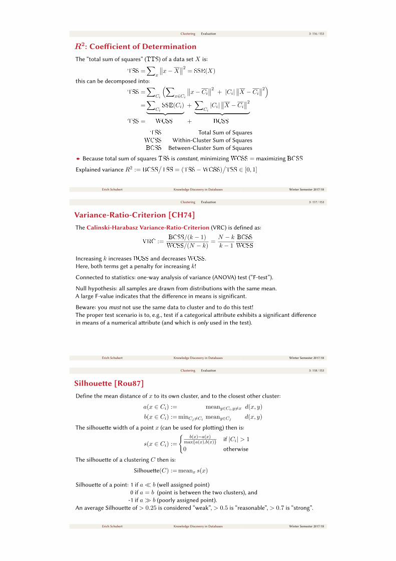
Clustering Evaluation 3: 116 / 153
R2: Coeicient of DeterminationThe “total sum of squares” (TTS) of a data set X is:
TSS =∑
x
∥∥x−X∥∥2= SSE(X)
this can be decomposed into:
TSS =∑
Ci
(∑x∈Ci
∥∥x− Ci∥∥2+ |Ci|
∥∥X − Ci∥∥2)
=∑
CiSSE(Ci)︸ ︷︷ ︸ +
∑Ci|Ci|
∥∥X − Ci∥∥2︸ ︷︷ ︸TSS = WCSS + BCSS
TSS Total Sum of Squares
WCSS Within-Cluster Sum of Squares
BCSS Between-Cluster Sum of Squares
z Because total sum of squares TSS is constant, minimizing WCSS = maximizing BCSS
Explained variance R2 := BCSS/TSS = (TSS−WCSS)
/TSS ∈ [0, 1]
Erich Schubert Knowledge Discovery in Databases Winter Semester 2017/18
Clustering Evaluation 3: 117 / 153
Variance-Ratio-Criterion [CH74]The Calinski-Harabasz Variance-Ratio-Criterion (VRC) is defined as:
VRC :=BCSS/(k − 1)
WCSS/(N − k)=N − kk − 1
BCSS
WCSS
Increasing k increases BCSS and decreases WCSS.
Here, both terms get a penalty for increasing k!
Connected to statistics: one-way analysis of variance (ANOVA) test (“F-test”).
Null hypothesis: all samples are drawn from distributions with the same mean.
A large F-value indicates that the dierence in means is significant.
Beware: you must not use the same data to cluster and to do this test!
The proper test scenario is to, e.g., test if a categorical aribute exhibits a significant dierence
in means of a numerical aribute (and which is only used in the test).
Erich Schubert Knowledge Discovery in Databases Winter Semester 2017/18
Clustering Evaluation 3: 118 / 153
Silhouee [Rou87]Define the mean distance of x to its own cluster, and to the closest other cluster:
a(x ∈ Ci) := meany∈Ci,y 6=x d(x, y)
b(x ∈ Ci) := minCj 6=Ci meany∈Cj d(x, y)
The silhouee width of a point x (can be used for ploing) then is:
s(x ∈ Ci) :=
b(x)−a(x)
maxa(x),b(x) if |Ci| > 1
0 otherwise
The silhouee of a clustering C then is:
Silhouee(C) := meanx s(x)
Silhouee of a point: 1 if a b (well assigned point)
0 if a = b (point is between the two clusters), and
-1 if a b (poorly assigned point).
An average Silhouee of > 0.25 is considered “weak”, > 0.5 is “reasonable”, > 0.7 is “strong”.
Erich Schubert Knowledge Discovery in Databases Winter Semester 2017/18

Clustering Evaluation 3: 119 / 153
Silhouee [Rou87] /2Challenges with using the Silhouee criterion:
I The complexity of Silhouee is: O(n2)⇒ does not scale to large data sets.
I Simplified Silhouee:
use the distances to cluster centers instead of average distances, O(n · k)
I When a cluster has a single point, a(x) is not defined.
Rousseeuw [Rou87] suggests to use s(x) = 0 then (see the definition of s(x))
I Which distance should we use, e.g., with k-means – Euclidean, or squared Euclidean?
I In high-dimensional data, a(x)→ b(x) due to the curse of dimensionality. Then s(x)→ 0
Erich Schubert Knowledge Discovery in Databases Winter Semester 2017/18
Clustering Evaluation 3: 120 / 153
Davies-Bouldin Index [DB79]Let the scaer of a cluster Ci be (recall Lp-norms):
Si :=(
1|Ci|
∑x∈Ci
‖x− µCi‖pp
)1/p
Let the separation of clusters be:
Mij :=∥∥µCi − µCj∥∥p
The similarity of two clusters then is defined as:
Rij :=Si+SjMij
Clustering quality is the average maximum similarity:
DB(C) := meanCi maxCj 6=Ci Rij
A small Davies-Bouldin index is beer, i.e., Si + Sj Mij , scaer distance
Power mean (with power p) of
(‖x− y‖p)p =
∑i(xi − yi)
p
For p = 2, Si is standard deviation,
Mij is the Euclidean distance!
Erich Schubert Knowledge Discovery in Databases Winter Semester 2017/18
Clustering Evaluation 3: 121 / 153
Other Internal Clustering IndexesThere have been many more indexes proposed over time:
I Dunn index: cluster distance / maximum cluster diameter [Dun73; Dun74]
I Gamma and Tau: P (within-cluster distance < between-cluster distance ) [BH75]
I C-Index: sum of within-cluster distances / same number of smallest distances [HL76]
I Xie-Beni index for fuzzy clustering [XB91]
I Gap statistic: compare to results on generated random data [TWH01]
I I-Index: maximum between cluster centers / sum of distances to the cluster center [MB02]
I S_Dbw: separation and density based [HV01; HBV02]
I PBM Index: distance to cluster center / distance to total center [PBM04]
I DBCV: density based cluster validation [Mou+14]
I . . .
Erich Schubert Knowledge Discovery in Databases Winter Semester 2017/18
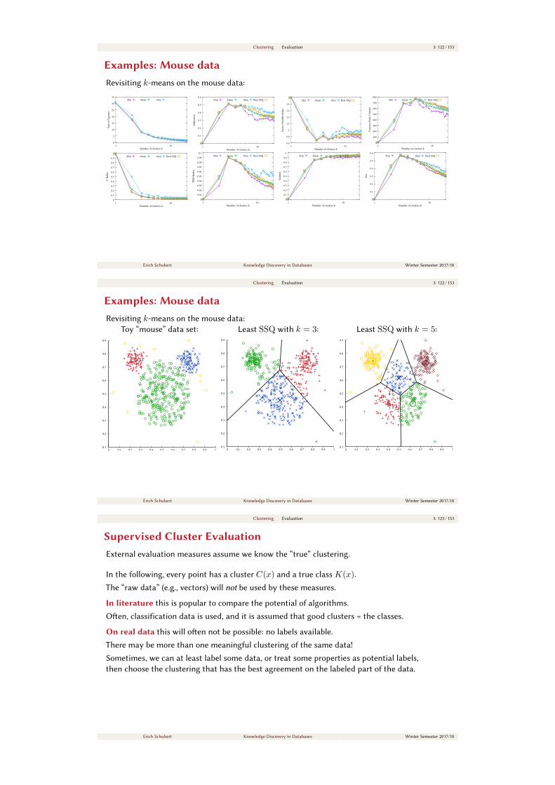
Clustering Evaluation 3: 122 / 153
Examples: Mouse dataRevisiting k-means on the mouse data:
0
5
10
15
20
25
30
35
1 10
Sum
of S
quar
es
Number of clusters k
Min Mean Max
0
0.1
0.2
0.3
0.4
0.5
0.6
1 10
Silh
oue
e
Number of clusters k
Min Mean Max Best SSQ
0.6
0.8
1
1.2
1.4
1.6
1.8
2
1 10
Dav
ies
Bou
ldin
Inde
x
Number of clusters k
Min Mean Max Best SSQ
0
100
200
300
400
500
600
700
800
1 10
Var
ianc
e R
atio
Cri
teri
a
Number of clusters k
Min Mean Max Best SSQ
0
0.1
0.2
0.3
0.4
0.5
0.6
0.7
0.8
0.9
1
1 10
C-I
ndex
Number of clusters k
Min Mean Max Best SSQ
0
0.01
0.02
0.03
0.04
0.05
0.06
0.07
0.08
0.09
0.1
1 10
PBM
-Ind
ex
Number of clusters k
Min Mean Max Best SSQ
0
0.1
0.2
0.3
0.4
0.5
0.6
0.7
0.8
0.9
1
1 10
Gam
ma
Number of clusters k
Min Mean Max Best SSQ
0
0.1
0.2
0.3
0.4
0.5
0.6
1 10
Tau
Number of clusters k
Min Mean Max Best SSQ
Erich Schubert Knowledge Discovery in Databases Winter Semester 2017/18
Clustering Evaluation 3: 122 / 153
Examples: Mouse dataRevisiting k-means on the mouse data:
Toy “mouse” data set:
0 0.1 0.2 0.3 0.4 0.5 0.6 0.7 0.8 0.9 10.1
0.2
0.3
0.4
0.5
0.6
0.7
0.8
0.9
Least SSQ with k = 3:
0 0.1 0.2 0.3 0.4 0.5 0.6 0.7 0.8 0.9 10.1
0.2
0.3
0.4
0.5
0.6
0.7
0.8
0.9
Least SSQ with k = 5:
0 0.1 0.2 0.3 0.4 0.5 0.6 0.7 0.8 0.9 10.1
0.2
0.3
0.4
0.5
0.6
0.7
0.8
0.9
Erich Schubert Knowledge Discovery in Databases Winter Semester 2017/18
Clustering Evaluation 3: 123 / 153
Supervised Cluster EvaluationExternal evaluation measures assume we know the “true” clustering.
In the following, every point has a cluster C(x) and a true class K(x).
The “raw data” (e.g., vectors) will not be used by these measures.
In literature this is popular to compare the potential of algorithms.
Oen, classification data is used, and it is assumed that good clusters = the classes.
On real data this will oen not be possible: no labels available.
There may be more than one meaningful clustering of the same data!
Sometimes, we can at least label some data, or treat some properties as potential labels,
then choose the clustering that has the best agreement on the labeled part of the data.
Erich Schubert Knowledge Discovery in Databases Winter Semester 2017/18
Clustering Evaluation 3: 124 / 153
Supervised Cluster Evaluation /2The matching problem:
I Clusters C are usually enumerated 1, 2, 3, . . . , k
I True classes K are usually labeled with meaningful classes
I Which C is which class K?
z Clustering is not classification, we cannot evaluate it the same way
I What if there are more clusters than classes?
I What if a cluster contains two classes?
I What if a class contains two clusters?
To overcome this
I Choose the best (C,K) matching with, e.g., the Hungarian algorithm (uncommon)
I Compare every cluster C to every class K
Erich Schubert Knowledge Discovery in Databases Winter Semester 2017/18
Clustering Evaluation 3: 125 / 153
Purity, Precision and RecallA simple measure popular in text clustering (but not much in “other” clustering):
Purity(Ci,K) := maxKj|Ci∩Kj ||Ci|
Purity(C,K) := 1N
∑i|Ci|Purity(Ci,K) = 1
N
∑imaxKj |Ci ∩Kj |
⇒ A cluster, which only contains elements of class Kj has purity 1z similar to “precision” in classification and information retrieval
But: every document is its own cluster has purity 1, is this really optimal?
We could also define a “recall” equivalent:
Recall(C,Kj) := maxCi|Ci∩Kj ||Kj |
Recall(C,K) := 1N
∑j|Kj |Recall(C,Kj) = 1
N
∑j
maxCi |Ci ∩Kj |
But this is even more misleading: if we put all objects into one cluster, we get recall 1!
Erich Schubert Knowledge Discovery in Databases Winter Semester 2017/18
Clustering Evaluation 3: 126 / 153
Pair-counting EvaluationMany cluster evaluation measures are based on pair-counting.
If (and only if) i and j are in the same cluster, then (i, j) is a pair.
This gives us a binary, classification-like problem:
K(i) = K(j): pair K(i) 6= K(j): no pair
C(i) = C(j) pair true positive (a) false positive (b)
C(i) 6= C(j) no pair false negative (c) true negative (d)
which can be computed using
a =∑
i,j
(|Ci∩Kj |2
)b =
∑i
(|Ci|2
)− a
c =∑
i
(|Ki|2
)− a d =
(N2
)− a− b− c
Objects are a “pair” i they are related (“should be together”)
z we are predicting which objects are related (pairs), and which are not
Erich Schubert Knowledge Discovery in Databases Winter Semester 2017/18

Clustering Evaluation 3: 127 / 153
Pair-counting Cluster Evaluation MeasuresK(i) = K(j): pair K(i) 6= K(j): no pair
C(i) = C(j) pair true positive (a) false positive (b)
C(i) 6= C(j) no pair false negative (c) true negative (d)
Precision = aa+b Recall = a
a+c
Rand index [Ran71] = a+da+b+c+d = (a+ d)/
(N2
)= Accuracy
Fowlkes-Mallows [FM83] =√Precision · Recall = a
/√(a+ b) · (a+ c)
Jaccard = aa+b+c
F1-Measure =2Precision·RecallPrecision+Recall
= 2a2a+b+c
Fβ-Measure = (1+β2)·Precision·Recallβ2·Precision+Recall
Adjusted Rand Index [HA85] = Rand index−E[Rand index]optimal Rand index−E[Rand index]
=(N2 )(a+d)−((a+b)(a+c)+(c+d)(b+d))
(N2 )2 −((a+b)(a+c)+(c+d)(b+d))
Erich Schubert Knowledge Discovery in Databases Winter Semester 2017/18
Clustering Evaluation 3: 128 / 153
Mutual Information [Mei03; Mei05; Mei12]Evaluation by Mutual Information:
I(C,K) =∑
i
∑jP (Ci ∩Kj) log
P (Ci ∩Kj)
P (Ci) · P (Kj)
=∑
i
∑j
|Ci ∩Kj |N
logN |Ci ∩Kj ||Ci| · |Kj |
Entropy:
H(C) =−∑
iP (Ci) logP (Ci) = −
∑i
|Ci|N
log|Ci|N
= I(C,C)
Normalized Mutual Information (NMI):10
NMI(C,K) =I(C,K)
(H(C) +H(K))/2=I(C,K) + I(K,C)
I(C,C) + I(K,K)
I and H are the usual Shannon entropy.
Using log ab
=− log ba
10
There exist ≥ 5 variations of normalized mutual information [VEB10].
Erich Schubert Knowledge Discovery in Databases Winter Semester 2017/18
Clustering Evaluation 3: 129 / 153
Further Supervised Cluster Evaluation MeasuresSome further evaluation measures:
I Adjustment for chance is general principle,
Adjusted Index = Index−E[Index]optimal Index−E[Index]
For example Adjusted Rand Index [HA85] or Adjusted Mutual Information [VEB10]
I B-Cubed evaluation [BB98]
I Set matching purity [ZK01] and F1 [SKK00]
I Edit distance [PL02]
I Visual comparison of multiple clusterings [Ach+12]
I Gini-based evaluation [Sch+15]
I . . .
Erich Schubert Knowledge Discovery in Databases Winter Semester 2017/18
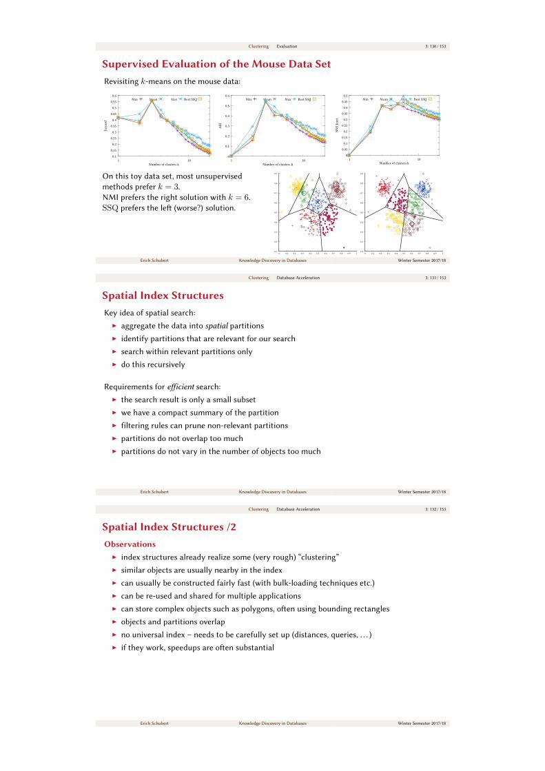
Clustering Evaluation 3: 130 / 153
Supervised Evaluation of the Mouse Data SetRevisiting k-means on the mouse data:
0.1
0.15
0.2
0.25
0.3
0.35
0.4
0.45
0.5
0.55
0.6
1 10
Jacc
ard
Number of clusters k
Min Mean Max Best SSQ
0
0.1
0.2
0.3
0.4
0.5
0.6
1 10
AR
I
Number of clusters k
Min Mean Max Best SSQ
0
0.05
0.1
0.15
0.2
0.25
0.3
0.35
0.4
0.45
0.5
1 10
NM
I Joi
nt
Number of clusters k
Min Mean Max Best SSQ
On this toy data set, most unsupervised
methods prefer k = 3.
NMI prefers the right solution with k = 6.
SSQ prefers the le (worse?) solution.
0 0.1 0.2 0.3 0.4 0.5 0.6 0.7 0.8 0.9 10.1
0.2
0.3
0.4
0.5
0.6
0.7
0.8
0.9
0 0.1 0.2 0.3 0.4 0.5 0.6 0.7 0.8 0.9 10.1
0.2
0.3
0.4
0.5
0.6
0.7
0.8
0.9
Erich Schubert Knowledge Discovery in Databases Winter Semester 2017/18
Clustering Database Acceleration 3: 131 / 153
Spatial Index StructuresKey idea of spatial search:
I aggregate the data into spatial partitions
I identify partitions that are relevant for our search
I search within relevant partitions only
I do this recursively
Requirements for eicient search:
I the search result is only a small subset
I we have a compact summary of the partition
I filtering rules can prune non-relevant partitions
I partitions do not overlap too much
I partitions do not vary in the number of objects too much
Erich Schubert Knowledge Discovery in Databases Winter Semester 2017/18
Clustering Database Acceleration 3: 132 / 153
Spatial Index Structures /2Observations
I index structures already realize some (very rough) “clustering”
I similar objects are usually nearby in the index
I can usually be constructed fairly fast (with bulk-loading techniques etc.)
I can be re-used and shared for multiple applications
I can store complex objects such as polygons, oen using bounding rectangles
I objects and partitions overlap
I no universal index – needs to be carefully set up (distances, queries, . . . )
I if they work, speedups are oen substantial
Erich Schubert Knowledge Discovery in Databases Winter Semester 2017/18

Clustering Database Acceleration 3: 133 / 153
Spatial Data Search: ε-Range eriesExample: summarize partitions using Minimum Bounding Rectangles (MBR):
q
MBR
MinDist(q,MBR)
Instead of computing the distances to each point, compute the minimum distance to the MBR.
If MinDist(q,MBR) > ε, then no point in the MBR can be closer than ε.
If MinDist(q,MBR) ≤ ε, we need to process the contents of the MBR.
Erich Schubert Knowledge Discovery in Databases Winter Semester 2017/18
Clustering Database Acceleration 3: 134 / 153
Spatial Data Search: k-Nearest NeighborsExample: ball cover:
q
r1p1r2
p2
MinDist(q, pi)c1,1
c2,1
Bounding sphere: for all child points cij of pi, we have dist(pi, cij) ≤ ri.
By the triangle inequality, we have dist(q, cij) + dist(cij , pi) ≥ dist(q, pi).
by using ri, we get the bound dist(q, cij) ≥ dist(q, pi)− dist(cij , pi) ≥ dist(q, pi)− riPut nodes pi into a priority queue, ordered by MinDist(q, pi) := dist(q, pi)− ri.If we have k results that are beer than the remaining queue entries, we can stop.
Balls will usually contain nested balls in a tree structure.
Erich Schubert Knowledge Discovery in Databases Winter Semester 2017/18
Clustering Database Acceleration 3: 135 / 153
Spatial Index StructuresMany dierent strategies for partitioning data exist:
I grid adtree [FB74], Gridfile [NHS84], . . .
I binary splits k-d-tree [Ben75], . . .
I minimal bounding boxes R-tree [Gut84], R+
-tree [SRF87], R∗-tree [Bec+90], . . .
I ball covers Ball-tree [Omo89], M-tree [CPZ97], iDistance[Yu+01],
Cover-tree [BKL06], . . .
I ball and outside VP-tree [Uhl91; Yia93], . . .
I . . .
Most use either rectangles (coordinate ranges), or balls (triangle inequality).
Simpler partition description = less data to read / process / update / . . . .
Erich Schubert Knowledge Discovery in Databases Winter Semester 2017/18
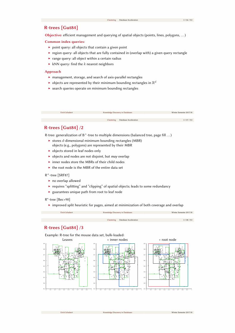
Clustering Database Acceleration 3: 136 / 153
R-trees [Gut84]Objective: eicient management and querying of spatial objects (points, lines, polygons, . . . )
Common index queries:I point query: all objects that contain a given point
I region query: all objects that are fully contained in (overlap with) a given query rectangle
I range query: all object within a certain radius
I kNN query: find the k nearest neighbors
ApproachI management, storage, and search of axis-parallel rectangles
I objects are represented by their minimum bounding rectangles in Rd
I search queries operate on minimum bounding rectangles
Erich Schubert Knowledge Discovery in Databases Winter Semester 2017/18
Clustering Database Acceleration 3: 137 / 153
R-trees [Gut84] /2R-tree: generalization of B
+-tree to multiple dimensions (balanced tree, page fill . . . )
I stores d-dimensional minimum bounding rectangles (MBR)
objects (e.g., polygons) are represented by their MBR
I objects stored in leaf nodes only
I objects and nodes are not disjoint, but may overlap
I inner nodes store the MBRs of their child nodes
I the root node is the MBR of the entire data set
R+
-tree [SRF87]
I no overlap allowed
I requires “spliing” and “clipping” of spatial objects; leads to some redundancy
I guarantees unique path from root to leaf node
R∗-tree [Bec+90]
I improved split heuristic for pages, aimed at minimization of both coverage and overlap
Erich Schubert Knowledge Discovery in Databases Winter Semester 2017/18
Clustering Database Acceleration 3: 138 / 153
R-trees [Gut84] /3Example: R-tree for the mouse data set, bulk-loaded:
Leaves
0 0.1 0.2 0.3 0.4 0.5 0.6 0.7 0.8 0.9 10.1
0.2
0.3
0.4
0.5
0.6
0.7
0.8
0.9
+ inner nodes
0 0.1 0.2 0.3 0.4 0.5 0.6 0.7 0.8 0.9 10.1
0.2
0.3
0.4
0.5
0.6
0.7
0.8
0.9
+ root node
0 0.1 0.2 0.3 0.4 0.5 0.6 0.7 0.8 0.9 10.1
0.2
0.3
0.4
0.5
0.6
0.7
0.8
0.9
Erich Schubert Knowledge Discovery in Databases Winter Semester 2017/18
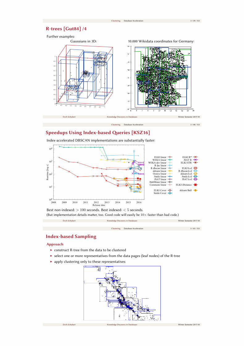
Clustering Database Acceleration 3: 139 / 153
R-trees [Gut84] /4Further examples:
Gaussians in 3D:
0 0.1 0.2 0.3 0.4 0.5 0.6 0.7 0.8 0.9 1
0
0.1
0.2
0.3
0.4
0.5
0.6
0.7
0.8
0.9
1
0
0.2
0.4
0.6
0.8
1
10.000 Wikidata coordinates for Germany:
Erich Schubert Knowledge Discovery in Databases Winter Semester 2017/18
Clustering Database Acceleration 3: 140 / 153
Speedups Using Index-based eries [KSZ16]Index-accelerated DBSCAN implementations are substantially faster:
100
101
102
103
104
2008 2009 2010 2011 2012 2013 2014 2015 2016
Run
tim
e [l
og s
]
Release date
ELKI linearWEKA linear
WEKA dev linearR fpc linear
R dbscan linearsklearn linearOctave linearSmile linearJSAT linear
HubMiner linearCommons linear
ELKI CoverSmile Cover
ELKI R*JSAT R
ELKI STR
ELKI k-dR dbscan k-d
sklearn k-dSmile k-dJSAT k-d
ELKI iDistance
sklearn Ball
Best non-indexed: > 100 seconds. Best indexed: < 5 seconds.
(But implementation details maer, too. Good code will easily be 10× faster than bad code.)
Erich Schubert Knowledge Discovery in Databases Winter Semester 2017/18
Clustering Database Acceleration 3: 141 / 153
Index-based SamplingApproach
I construct R-tree from the data to be clustered
I select one or more representatives from the data pages (leaf nodes) of the R-tree
I apply clustering only to these representatives
183Knowledge Discovery in Datenbanken
Kapitel 4 – Externspeicherbasiertes Clustering! Prof. Dr.-Ing. Wolfgang LehnerTU Dresden (Datenbanksysteme)
4.3 INDEXBASIERTES SAMPLING
! Verfahren
• Falls nicht ohnehin vorhanden, erstelle mit den zu clusternden Daten einen R-Baum
• Wähle von den Datenseiten des R-Baums einen oder mehrere Repräsentanten
• Wende das Clustering-Verfahren nur auf diese Repräsentantenmenge an
184Knowledge Discovery in Datenbanken
Kapitel 4 – Externspeicherbasiertes Clustering! Prof. Dr.-Ing. Wolfgang LehnerTU Dresden (Datenbanksysteme)
Ansatz der indexbasierten Sampling-Methode
! Beobachtung
• Repräsentative Objekte von den Datenseiten eines R*-Baums ergeben “so gut wiesicher” eine gut verteilte Stichprobe!
! Problem: Vom Stichproben-Clustering zum Clustering der Gesamtmenge
• k-means und k-mediod Verfahren• Repräsentanten der Cluster (Centroide, Medoide) werden für die gesamte Datenmenge
übernommen
• Dichtebasierte Verfahren• Bildung einer Repräsentation der Cluster (z.B. (Mengen von) minimal-umgebende(n)
Hyperrechtecke(n) oder repräsentative Punkte)
• Zuweisung der Objekte dem “besten” (d.h. dem nächstliegenden) der gefundenen Clusterzugewiesen
• Bei hierarchischen Verfahren• ?
Erich Schubert Knowledge Discovery in Databases Winter Semester 2017/18
Clustering Database Acceleration 3: 142 / 153
Bibliography I[Ach+12] Elke Achtert, Sascha Goldhofer, Hans-Peter Kriegel, Erich Schubert, and Arthur Zimek. “Evaluation of Clusterings -
Metrics and Visual Support”. In: IEEE ICDE. 2012, pp. 1285–1288.
[Agg+99] C. C. Aggarwal, C. M. Procopiuc, J. L. Wolf, P. S. Yu, and J. S. Park. “Fast Algorithms for Projected Clustering”. In: Proc.ACM SIGMOD International Conference on Management of Data. 1999, pp. 61–72.
[Agr+98] R. Agrawal, J. Gehrke, D. Gunopulos, and P. Raghavan. “Automatic Subspace Clustering of High Dimensional Data for
Data Mining Applications”. In: SIGMOD. 1998, pp. 94–105.
[Aka77] H. Akaike. “On entropy maximization principle”. In: Applications of Statistics. 1977, pp. 27–41.
[And73] M. R. Anderberg. “Cluster analysis for applications”. In: Probability and mathematical statistics. Academic Press, 1973.
Chap. Hierarchical Clustering Methods, pp. 131–155. isbn: 0120576503.
[Ank+99] M. Ankerst, M. M. Breunig, H.-P. Kriegel, and J. Sander. “OPTICS: Ordering Points To Identify the Clustering
Structure”. In: SIGMOD 1999. 1999, pp. 49–60.
[AV06] David Arthur and Sergei Vassilvitskii. “How slow is the k-means method?” In: Symposium on Computational Geometry.
2006, pp. 144–153.
[AV07] D. Arthur and S. Vassilvitskii. “k-means++: the advantages of careful seeding”. In: ACM-SIAM Symposium on DiscreteAlgorithms (SODA). 2007, pp. 1027–1035.
[Ban+05] Arindam Banerjee, Srujana Merugu, Inderjit S. Dhillon, and Joydeep Ghosh. “Clustering with Bregman Divergences”.
In: J. Machine Learning Research 6 (2005), pp. 1705–1749.
Erich Schubert Knowledge Discovery in Databases Winter Semester 2017/18
Clustering Database Acceleration 3: 143 / 153
Bibliography II[BB98] A. Bagga and B. Baldwin. “Entity-Based Cross-Document Coreferencing Using the Vector Space Model”. In:
COLING-ACL. 1998, pp. 79–85.
[Bec+90] Norbert Beckmann, Hans-Peter Kriegel, Ralf Schneider, and Bernhard Seeger. “The R*-Tree: An Eicient and Robust
Access Method for Points and Rectangles”. In: SIGMOD 1990. 1990, pp. 322–331.
[Ben75] Jon Louis Bentley. “Multidimensional Binary Search Trees Used for Associative Searching”. In: Commun. ACM 18.9
(1975), pp. 509–517.
[Bez81] James C. Bezdek. Paern Recognition with Fuzzy Objective Function Algorithms. Springer, 1981.
[BH65] G. H. Ball and D. J. Hall. ISODATA, a novel method of data analysis and paern classification. Tech. rep. Stanford
Research Institute, 1965.
[BH75] F. B. Baker and L. J. Hubert. “Measuring the Power of Hierarchical Cluster Analysis”. In: Journal American StatisticalAssociation 70.349 (1975), pp. 31–38.
[BKL06] Alina Beygelzimer, Sham Kakade, and John Langford. “Cover trees for nearest neighbor”. In: ICML. 2006, pp. 97–104.
[BMS96] Paul S. Bradley, Olvi L. Mangasarian, and W. Nick Street. “Clustering via Concave Minimization”. In: NIPS. 1996,
pp. 368–374.
[Boc07] H.-H. Bock. “Clustering Methods: A History of k-Means Algorithms”. In: Selected Contributions in Data Analysis andClassification. Ed. by P. Brito, G. Cucumel, P. Bertrand, and F. Carvalho. Springer, 2007, pp. 161–172.
[Bon64] Raymond E. Bonner. “On Some Clustering Techniques”. In: IBM Journal of Research and Development 8.1 (1964),
pp. 22–32.
Erich Schubert Knowledge Discovery in Databases Winter Semester 2017/18
Clustering Database Acceleration 3: 144 / 153
Bibliography III[Bre+01] M. M. Breunig, H.-P. Kriegel, P. Kröger, and J. Sander. “Data Bubbles: ality Preserving Performance Boosting for
Hierarchical Clustering”. In: SIGMOD. 2001, pp. 79–90.
[BY07] E. Biçici and D. Yuret. “Locally Scaled Density Based Clustering”. In: ICANNGA 2007. 2007, pp. 739–748.
[Cad+03] Igor V. Cadez, David Heckerman, Christopher Meek, Padhraic Smyth, and Steven White. “Model-Based Clustering and
Visualization of Navigation Paerns on a Web Site”. In: Data Min. Knowl. Discov. 7.4 (2003), pp. 399–424.
[Cam+13] R. J. G. B. Campello, D. Moulavi, A. Zimek, and J. Sander. “A framework for semi-supervised and unsupervised optimal
extraction of clusters from hierarchies”. In: Data Min. Knowl. Discov. 27.3 (2013), pp. 344–371.
[CC00] Y. Cheng and G. M. Church. “Biclustering of Expression Data”. In: ISMB. 2000, pp. 93–103.
[CH74] T. Caliński and J. Harabasz. “A dendrite method for cluster analysis”. In: Communications in Statistics 3.1 (1974),
pp. 1–27.
[Chi+01] T. Chiu, D. Fang, J. Chen, Y. Wang, and C. Jeris. “A robust and scalable clustering algorithm for mixed type aributes in
large database environment”. In: SIGKDD. 2001, pp. 263–268.
[CMS13] R. J. G. B. Campello, D. Moulavi, and J. Sander. “Density-Based Clustering Based on Hierarchical Density Estimates”.
In: PAKDD. 2013, pp. 160–172.
[CPZ97] Paolo Ciaccia, Marco Patella, and Pavel Zezula. “M-tree: An Eicient Access Method for Similarity Search in Metric
Spaces”. In: VLDB. 1997, pp. 426–435.
[DB79] D. Davies and D. Bouldin. “A cluster separation measure”. In: Paern Analysis and Machine Intelligence 1 (1979),
pp. 224–227.
Erich Schubert Knowledge Discovery in Databases Winter Semester 2017/18

Clustering Database Acceleration 3: 145 / 153
Bibliography IV[DD09] M. M. Deza and E. Deza. Encyclopedia of Distances. 3rd. Springer, 2009. isbn: 9783662443415.
[DE84] William H. E. Day and Herbert Edelsbrunner. “Eicient algorithms for agglomerative hierarchical clustering methods”.
In: Journal of Classification 1.1 (1984), pp. 7–24.
[Def77] D. Defays. “An Eicient Algorithm for the Complete Link Cluster Method”. In: The Computer Journal 20.4 (1977),
pp. 364–366.
[DLR77] A. P. Dempster, N. M. Laird, and D. B. Rubin. “Maximum Likelihood from Incomplete Data via the EM algorithm”. In:
Journal of the Royal Statistical Society: Series B (Statistical Methodology) 39.1 (1977), pp. 1–31.
[DM01] Inderjit S. Dhillon and Dharmendra S. Modha. “Concept Decompositions for Large Sparse Text Data Using Clustering”.
In: Machine Learning 42.1/2 (2001), pp. 143–175.
[Dun73] J. C. Dunn. “A Fuzzy Relative of the ISODATA Process and Its Use in Detecting Compact Well-Separated Clusters”. In:
Journal of Cybernetics 3.3 (1973), pp. 32–57.
[Dun74] J. C. Dunn. “Well separated clusters and optimal fuzzy partitions”. In: Journal of Cybernetics 4 (1974), pp. 95–104.
[Epp98] David Eppstein. “Fast Hierarchical Clustering and Other Applications of Dynamic Closest Pairs”. In: Proc. ACM-SIAMSymposium on Discrete Algorithms. 1998, pp. 619–628.
[Est+96] M. Ester, H.-P. Kriegel, J. Sander, and X. Xu. “A Density-Based Algorithm for Discovering Clusters in Large Spatial
Databases with Noise”. In: KDD’96. 1996, pp. 226–231.
[Est02] V. Estivill-Castro. “Why so many clustering algorithms – A Position Paper”. In: SIGKDD Explorations 4.1 (2002),
pp. 65–75.
Erich Schubert Knowledge Discovery in Databases Winter Semester 2017/18
Clustering Database Acceleration 3: 146 / 153
Bibliography V[FB74] Raphael A. Finkel and Jon Louis Bentley. “ad Trees: A Data Structure for Retrieval on Composite Keys”. In: Acta Inf.
4 (1974), pp. 1–9.
[FD07] B. J. Frey and D. Dueck. “Clustering by passing messages between data points”. In: Science 315.5814 (2007), pp. 972–976.
[FH75] K. Fukunaga and L. D. Hostetler. “The estimation of the gradient of a density function, with applications in paern
recognition”. In: IEEE Trans. Information Theory 21.1 (1975), pp. 32–40.
[FM83] E. B. Fowlkes and C. L. Mallows. “A Method for Comparing Two Hierarchical Clusterings”. In: Journal AmericanStatistical Association 78.383 (1983), pp. 553–569.
[For65] E. W. Forgy. “Cluster analysis of multivariate data: eiciency versus interpretability of classifications”. In: Biometrics 21
(1965), pp. 768–769.
[GRS98] S. Guha, R. Rastogi, and K. Shim. “CURE: An Eicient Clustering Algorithm for Large Databases”. In: SIGMOD. 1998,
pp. 73–84.
[GRS99] S. Guha, R. Rastogi, and K. Shim. “ROCK: A Robust Clustering Algorithm for Categorical Aributes”. In: ICDE. 1999,
pp. 512–521.
[Gut84] Antonin Guman. “R-Trees: A Dynamic Index Structure for Spatial Searching”. In: SIGMOD’84. 1984, pp. 47–57.
[HA85] L. Hubert and P. Arabie. “Comparing partitions”. In: Journal of Classification 2.1 (1985), pp. 193–218.
[Har75] J. A. Hartigan. Clustering Algorithms. New York, London, Sydney, Toronto: John Wiley&Sons, 1975.
[HBV02] Maria Halkidi, Yannis Batistakis, and Michalis Vazirgiannis. “Clustering Validity Checking Methods: Part II”. In:
SIGMOD Record 31.3 (2002), pp. 19–27.
Erich Schubert Knowledge Discovery in Databases Winter Semester 2017/18
Clustering Database Acceleration 3: 147 / 153
Bibliography VI[HE03] Greg Hamerly and Charles Elkan. “Learning the k in k-means”. In: NIPS. 2003, pp. 281–288.
[HG07] A. Hinneburg and H.-H. Gabriel. “DENCLUE 2.0: Fast Clustering Based on Kernel Density Estimation”. In: Advances inIntelligent Data Analysis VII. 2007, pp. 70–80.
[HK98] A. Hinneburg and D. A. Keim. “An Eicient Approach to Clustering in Large Multimedia Databases with Noise”. In:
KDD’98. 1998, pp. 58–65.
[HL76] L. J. Hubert and J. R. Levin. “A general statistical framework for assessing categorical clustering in free recall.” In:
Psychological Bulletin 83.6 (1976), pp. 1072–1080.
[Hof99] Thomas Hofmann. “Learning the Similarity of Documents: An Information-Geometric Approach to Document
Retrieval and Categorization”. In: Neural Information Processing Systems, NIPS. 1999, pp. 914–920.
[Hua98] Zhexue Huang. “Extensions to the k-Means Algorithm for Clustering Large Data Sets with Categorical Values”. In:
Data Min. Knowl. Discov. 2.3 (1998), pp. 283–304.
[HV01] M. Halkidi and M. Vazirgiannis. “Clustering Validity Assessment: Finding the Optimal Partitioning of a Data Set”. In:
ICDM. 2001, pp. 187–194.
[HW79] J. A. Hartigan and M. A. Wong. “Algorithm AS 136: A k-means clustering algorithm”. In: Journal of the Royal StatisticalSociety: Series C (Applied Statistics) (1979), pp. 100–108.
[KHK99] G. Karypis, E.-H. Han, and V. Kumar. “Chameleon: Hierarchical Clustering Using Dynamic Modeling”. In: IEEEComputer 32.8 (1999), pp. 68–75.
Erich Schubert Knowledge Discovery in Databases Winter Semester 2017/18
Clustering Database Acceleration 3: 148 / 153
Bibliography VII[KKK04] P. Kröger, H.-P. Kriegel, and K. Kailing. “Density-Connected Subspace Clustering for High-Dimensional Data”. In: Proc.
of the Fourth SIAM International Conference on Data Mining. 2004, pp. 246–256.
[KR90] L. Kaufman and P. J. Rousseeuw. Finding Groups in Data: An Introduction to Cluster Analyis. John Wiley&Sons, 1990.
isbn: 9780471878766.
[KSZ16] H.-P. Kriegel, E. Schubert, and A. Zimek. “The (black) art of runtime evaluation: Are we comparing algorithms or
implementations?” In: Knowledge and Information Systems (KAIS) (2016), pp. 1–38.
[Llo82] S. P. Lloyd. “Least squares quantization in PCM”. In: IEEE Transactions on Information Theory 28.2 (1982), pp. 129–136.
[LW67] G. N. Lance and W. T. Williams. “A General Theory of Classificatory Sorting Strategies. 1. Hierarchical Systems”. In:
The Computer Journal 9.4 (1967), pp. 373–380.
[Mac67] J. Maceen. “Some Methods for Classification and Analysis of Multivariate Observations”. In: 5th BerkeleySymposium on Mathematics, Statistics, and Probabilistics. Vol. 1. 1967, pp. 281–297.
[MAS16] S. T. Mai, I. Assent, and M. Storgaard. “AnyDBC: An Eicient Anytime Density-based Clustering Algorithm for Very
Large Complex Datasets”. In: KDD 2016. 2016, pp. 1025–1034.
[MB02] Ujjwal Maulik and Sanghamitra Bandyopadhyay. “Performance Evaluation of Some Clustering Algorithms and
Validity Indices”. In: IEEE Trans. Paern Anal. Mach. Intell. 24.12 (2002), pp. 1650–1654.
[Mei03] M. Meila. “Comparing Clusterings by the Variation of Information”. In: Computational Learning Theory (COLT). 2003,
pp. 173–187.
[Mei05] M. Meila. “Comparing Clusterings – An Axiomatic View”. In: Int. Conf. Machine Learning (ICML). 2005, pp. 577–584.
Erich Schubert Knowledge Discovery in Databases Winter Semester 2017/18
Clustering Database Acceleration 3: 149 / 153
Bibliography VIII[Mei12] M. Meilă. “Local equivalences of distances between clusterings–a geometric perspective”. In: Machine Learning 86.3
(2012), pp. 369–389.
[MM08] S. Mahran and K. Mahar. “Using grid for accelerating density-based clustering”. In: CIT 2008. 2008, pp. 35–40.
[Mou+14] D. Moulavi, P. A. Jaskowiak, R. J. G. B. Campello, A. Zimek, and J. Sander. “Density-based Clustering Validation”. In:
SIAM SDM. 2014, pp. 839–847.
[MS00] M. Meila and J. Shi. “Learning Segmentation by Random Walks”. In: NIPS. MIT Press, 2000, pp. 873–879.
[Mül11] D. Müllner. “Modern hierarchical, agglomerative clustering algorithms”. In: arXiv preprint arXiv:1207.0016 (2011).
[Mur83] F. Murtagh. “A Survey of Recent Advances in Hierarchical Clustering Algorithms”. In: Comput. J. 26.4 (1983),
pp. 354–359.
[NH02] R. T. Ng and J. Han. “CLARANS: A method for clustering objects for spatial data mining”. In: IEEE Transactions onKnowledge and Data Engineering 14.5 (2002), pp. 1003–1016.
[NHS84] Jürg Nievergelt, Hans Hinterberger, and Kenneth C. Sevcik. “The Grid File: An Adaptable, Symmetric Multikey File
Structure”. In: ACM Trans. Database Syst. 9.1 (1984), pp. 38–71.
[NJW01] A. Y. Ng, M. I. Jordan, and Y. Weiss. “On Spectral Clustering: Analysis and an algorithm”. In: NIPS. 2001, pp. 849–856.
[Omo89] Stephen M. Omohundro. Five Balltree Construction Algorithms. Tech. rep. TR-89-063. International Computer Science
Institute, Berkeley, 1989.
[PBM04] M. K. Pakhira, S. Bandyopadhyay, and U. Maulik. “Validity index for crisp and fuzzy clusters”. In: Paern Recognition37.3 (2004), pp. 487–501.
Erich Schubert Knowledge Discovery in Databases Winter Semester 2017/18
Clustering Database Acceleration 3: 150 / 153
Bibliography IX[Phi02] S. J. Phillips. “Acceleration of K-Means and Related Clustering Algorithms”. In: ALENEX’02. 2002, pp. 166–177.
[PL02] P. Pantel and D. Lin. “Document clustering with commiees”. In: ACM SIGIR. 2002, pp. 199–206.
[PM00] D. Pelleg and A. Moore. “X-means: Extending k-means with eicient estimation of the number of clusters”. In:
Proceedings of the 17th International Conference on Machine Learning (ICML). Vol. 1. 2000, pp. 727–734.
[Pou+14] M. Pourrajabi, D. Moulavi, R. J. G. B. Campello, A. Zimek, J. Sander, and R. Goebel. “Model Selection for
Semi-Supervised Clustering”. In: EDBT 2014. 2014, pp. 331–342.
[Ran71] W. M. Rand. “Objective criteria for the evaluation of clustering methods”. In: Journal American Statistical Association66.336 (1971), pp. 846–850.
[RL14] A. Rodriguez and A. Laio. “Clustering by fast search and find of density peaks”. In: Science 344.6191 (2014),
pp. 1492–1496.
[Rou87] P. J. Rousseeuw. “Silhouees: a graphical aid to the interpretation and validation of cluster analysis”. In: Journal ofcomputational and applied mathematics 20 (1987), pp. 53–65.
[San+98] J. Sander, M. Ester, H.-P. Kriegel, and X. Xu. “Density-Based Clustering in Spatial Databases: The Algorithm GDBSCAN
and Its Applications”. In: Data Min. Knowl. Discov. 2.2 (1998), pp. 169–194.
[Sch+15] E. Schubert, A. Koos, T. Emrich, A. Züfle, K. A. Schmid, and A. Zimek. “A Framework for Clustering Uncertain Data”. In:
Proceedings of the VLDB Endowment 8.12 (2015), pp. 1976–1979.
[Sch+17a] E. Schubert, J. Sander, M. Ester, H.-P. Kriegel, and X. Xu. “DBSCAN Revisited, Revisited: Why and How You Should
(Still) Use DBSCAN”. In: ACM Trans. Database Syst. 42.3 (2017), 19:1–19:21.
Erich Schubert Knowledge Discovery in Databases Winter Semester 2017/18

Clustering Database Acceleration 3: 151 / 153
Bibliography X[Sch+17b] E. Schubert, A. Spitz, M. Weiler, J. Geiß, and M. Gertz. “Semantic Word Clouds with Background Corpus
Normalization and t-distributed Stochastic Neighbor Embedding”. In: CoRR abs/1708.03569 (2017). arXiv: 1708.03569.
[Sch78] G. Schwarz. “Estimating the dimension of a model”. In: The Annals of Statistics 6.2 (1978), pp. 461–464.
[Sib73] R. Sibson. “SLINK: An Optimally Eicient Algorithm for the Single-Link Cluster Method”. In: The Computer Journal 16.1
(1973), pp. 30–34.
[SKK00] M. Steinbach, G. Karypis, and V. Kumar. “A comparison of document clustering techniques”. In: KDD workshop on textmining. Vol. 400. 2000, pp. 525–526.
[SM00] J. Shi and J. Malik. “Normalized Cuts and Image Segmentation”. In: IEEE Trans. Paern Anal. Mach. Intell. 22.8 (2000),
pp. 888–905.
[Sne57] P. H. A. Sneath. “The Application of Computers to Taxonomy”. In: Journal of General Microbiology 17 (1957),
pp. 201–226.
[SRF87] Timos K. Sellis, Nick Roussopoulos, and Christos Faloutsos. “The R+-Tree: A Dynamic Index for Multi-Dimensional
Objects”. In: VLDB’87. 1987, pp. 507–518.
[Ste56] H. Steinhaus. “Sur la division des corp materiels en parties”. In: Bull. Acad. Polon. Sci 1 (1956), pp. 801–804.
[TWH01] Robert Tibshirani, Guenther Walther, and Trevor Hastie. “Estimating the number of clusters in a data set via the gap
statistic”. In: Journal of the Royal Statistical Society: Series B (Statistical Methodology) 63.2 (2001), pp. 411–423.
[Uhl91] Jerey K. Uhlmann. “Satisfying General Proximity/Similarity eries with Metric Trees”. In: Inf. Process. Le. 40.4
(1991), pp. 175–179.
Erich Schubert Knowledge Discovery in Databases Winter Semester 2017/18
Clustering Database Acceleration 3: 152 / 153
Bibliography XI[VEB10] N. X. Vinh, J. Epps, and J. Bailey. “Information Theoretic Measures for Clustering Comparison: Variants, Properties,
Normalization and Correction for Chance”. In: J. Machine Learning Research 11 (2010), pp. 2837–2854.
[XB91] Xuanli Lisa Xie and Gerardo Beni. “A Validity Measure for Fuzzy Clustering”. In: IEEE Trans. Paern Anal. Mach. Intell.13.8 (1991), pp. 841–847.
[YH02] Alexander Ypma and Tom Heskes. “Automatic Categorization of Web Pages and User Clustering with Mixtures of
Hidden Markov Models”. In: Workshop WEBKDD. 2002, pp. 35–49.
[Yia93] Peter N. Yianilos. “Data Structures and Algorithms for Nearest Neighbor Search in General Metric Spaces”. In: SODA1993. 1993, pp. 311–321.
[Yu+01] Cui Yu, Beng Chin Ooi, Kian-Lee Tan, and H. V. Jagadish. “Indexing the Distance: An Eicient Method to KNN
Processing”. In: VLDB. 2001, pp. 421–430.
[ZK01] Y. Zhao and G. Karypis. Criterion Functions for Document Clustering: Experiments and Analysis. Tech. rep. 01-40.
University of Minnesota, Department of Computer Science, 2001.
[ZRL96] T. Zhang, R. Ramakrishnan, and M. Livny. “BIRCH: An Eicient Data Clustering Method for Very Large Databases”. In:
SIGMOD 1996. 1996, pp. 103–114.
[ZXF08] Q. Zhao, M. Xu, and P. Fränti. “Knee Point Detection on Bayesian Information Criterion”. In: IEEE InternationalConference on Tools with Artificial Intelligence (ICTAI). 2008, pp. 431–438.
Erich Schubert Knowledge Discovery in Databases Winter Semester 2017/18