konya i. lectures notes in international trade (boston, 2001)(118s)_gi
TRANSCRIPT
8/20/2019 Konya I. Lectures Notes in International Trade (Boston, 2001)(118s)_GI
http://slidepdf.com/reader/full/konya-i-lectures-notes-in-international-trade-boston-2001118sgi 1/118
Lecture notes in International Trade
Istvan KonyaDept. of Economics
Boston College
Fall 2001
8/20/2019 Konya I. Lectures Notes in International Trade (Boston, 2001)(118s)_GI
http://slidepdf.com/reader/full/konya-i-lectures-notes-in-international-trade-boston-2001118sgi 2/118
Introduction
What is international trade theory?
International trade theory is basically an exercise in applied general equi-librium modeling. This means that in many cases one can use the generaltheorems that apply for any Arrow-Debreu economy, most notably aboutthe existence and welfare properties of equilibria. What makes internationaltrade a separate field is that it utilizes some assumptions that allow for muchsharper positive and normative results than what are possible in the theoryof general equilibrium (hence the phrase “applied”).
What are the special assumptions? Since there are many different mod-els, let us try to summarize the common elements. The most basic postulateis that the world consists of separate geographic entities (regions or coun-tries). Goods and factors of production are more mobile within countries
than among them, because of physical, political and psychological barriersof movement. In most models factors and goods are perfectly mobile withincountries, but factors are immobile across borders. The mobility of goodsacross countries is an important variable, and ranges from none (autarchy)to complete (free trade). Some of the basic results in trade theory come fromanalyzing the effect of goods mobility.
Questions and answers
A good theory has both positive and normative applications, and interna-
tional trade is usually useful for both purposes. The most important ques-tions in trade theory include the following:
Positive:
i

8/20/2019 Konya I. Lectures Notes in International Trade (Boston, 2001)(118s)_GI
http://slidepdf.com/reader/full/konya-i-lectures-notes-in-international-trade-boston-2001118sgi 3/118
ii
• Why do nations trade?
• What do they trade?
• Can we use a small set of parameters to predict trade flows?
• What is the effect of trade barriers on trade?
• Why do the man-made trade barriers exist?
• Can trade in goods substitute for factor mobility?
• What is the effect of trade on factor rewards?
Normative:
• Is free trade better than autarchy?
• Is free trade optimal for a country?
• What are the effects of trade on income distribution?
• If there are winners and losers, can the former compensate the latter?
• If nations gain from trade, how are the gains distributed?
• If we change parameters, how are these gains redistributed, both withinand across countries?
• What are the welfare effects of various trade policies?
The most basic question is probably the first one, why do nations trade?There are three possible answers yet: comparative advantage , division of labor
and oligopolistic conduct . The first concept, originated by David Ricardo, isone of the nicest insights in economics. It roughly says that trade is due toautarchy price differences. Because of differences in the underlying param-eters, some countries can produce some goods relatively more efficiently, sowhen trade is allowed they will specialize in those goods. Good anecdotes
abound, for example the professor and the secretary1. Much of traditional1The story is as follows. Suppose the professor is more productive in both research and
envelope stuffing than the secretary. Still, if his advantage is relatively bigger in research,he should specialize in it and leave envelopes to the secretary.
8/20/2019 Konya I. Lectures Notes in International Trade (Boston, 2001)(118s)_GI
http://slidepdf.com/reader/full/konya-i-lectures-notes-in-international-trade-boston-2001118sgi 4/118
iii
trade theory is concerned with explaining the cause of autarchy price differ-
ences. Candidates include technology, factor endowments and tastes.The second concept is even older, and (like almost everything in eco-nomics) goes back to Adam Smith. His idea was that nations trade in orderto exploit economies of scale that arise from specialization. The finer thedivision of labor is, the richer countries are. By increasing the size of themarket, trade allows for more specialization, and hence leads to gains for theparticipants. This argument, in contrast to comparative advantage, workseven if the trading countries are identical in all respects. This explains whyit received much attention in the last two decades, when trade is increasinglyamong seemingly similar countries. In fact specialization due to increasingreturns forms the basis for most of the “New Trade Theory”.
The third concept is fairly recent, and it was first advanced by JamesBrander in the early ’80s. While specialization explains trade in similar butdifferentiated products, oligopolies can lead to trade in identical goods. If,for example, two firms in two countries compete in a Cournot-setting, theywill export to each other’s markets even if their products are identical. If there are transportation costs, firms will charge a lower price abroad than athome, which can lead to reciprocal dumping . While theoretically intriguing,trade in identical products and reciprocal dumping are usually thought tobe less important in explaining trade than comparative advantage and spe-cialization. Nevertheless, such models yield useful insights that should beincorporated in a general model of trade.
Plan of the course
Most of the course will be about answering the positive questions, althoughwe will venture a little into the normative ones. The first part will focus oncomparative advantage, or the “classical” theory of trade. Twenty-five yearsago this was pretty much the trade theory, and it still forms the backboneof the field. We will inquire into the questions about the pattern of trade,income distribution, factor rewards etc. There are various interesting specialcases that received much attention, and we will look at them in some detail.We will also summarize some of the evidence about trade models based oncomparative advantage, and the Heckscher-Ohlin model in particular. Aswe will see, there is fairly solid support for the theory in general, but onceone looks at the data in more detail, many puzzling questions emerge. Thus

8/20/2019 Konya I. Lectures Notes in International Trade (Boston, 2001)(118s)_GI
http://slidepdf.com/reader/full/konya-i-lectures-notes-in-international-trade-boston-2001118sgi 5/118
iv
there is a more or less general consensus among researchers that comparative
advantage is an important, but partial explanation for international trade.The second part of the course will deal with “New Trade Theory”. Mostof it elaborates the division of labor explanation for trade, with a detourtowards oligopolies and reciprocal dumping. As we will see, comparativeadvantage and increasing returns can coexist peacefully, each explaining adifferent pattern of the data. There is some supportive evidence for thisricher model, presented at the end of the topic. An important branch of “New Trade Theory” is the “New Economic Geography”, that is concernedabout the location of economic activity. It is a fascinating topic, althoughit is a bit easy to get carried away. Nevertheless, it deserves some seriousattention.
Most of trade theory is essentially static. There are some questions,however, that require us to explicitly consider dynamics. First, in many casescomparative advantage seems to be acquired, and not given by unchangingfundamentals. Thus we will incorporate learning-by-doing into trade models,and see how specialization emerges in the long run. Second, trade can have alarge influence on economic growth. Open economy extensions of endogenousgrowth theory shed some light on how international trade and growth arerelated, and we will study such models. Third, much of trade (and evenmore trade policy debate) is between rich and poor countries, thus we willlook at models of North-South trade. Finally, some evidence will be presentedabout the connections among trade, technology and growth.
The last topic can be thought of as an exercise in applying the toolslearned in the first three parts. The world seems to be more and more pre-occupied by “globalization”, and who else but trade theorists can providesome insight into the debate. We will limit ourselves to questions that in-terested researchers in the rich world. Much attention has been focused onthe trinity of immigration, trade and factor prices (wages). There is ampleevidence in the US (and also in some other industrial countries) of increasingwage inequality, which coincides with globalization in the last two or threedecades. Thus this part will mainly look at theory and evidence on howimmigration, trade and wages are related. There is no definite answer yet,
but it is important to understand the framework of the debate, and - as Isaid - it is also a good exercise.
8/20/2019 Konya I. Lectures Notes in International Trade (Boston, 2001)(118s)_GI
http://slidepdf.com/reader/full/konya-i-lectures-notes-in-international-trade-boston-2001118sgi 6/118
Contents
I The classical theory of international trade 1
1 Basic issues 2
1.1 Comparative advantage with two goods . . . . . . . . . . . . . 21.2 Explaining comparative advantage . . . . . . . . . . . . . . . . 3
2 Analytical tools 6
2.1 The revenue function . . . . . . . . . . . . . . . . . . . . . . . 62.2 The cost function . . . . . . . . . . . . . . . . . . . . . . . . . 72.3 Consumer choice . . . . . . . . . . . . . . . . . . . . . . . . . 92.4 The Meade utility functions . . . . . . . . . . . . . . . . . . . 10
3 Equilibrium and the gains from trade 11
3.1 Defining the equilibrium . . . . . . . . . . . . . . . . . . . . . 11
3.2 Gains from trade . . . . . . . . . . . . . . . . . . . . . . . . . 12
4 Factor price equalization 15
4.1 General results . . . . . . . . . . . . . . . . . . . . . . . . . . 154.1.1 Comparative advantage . . . . . . . . . . . . . . . . . . 154.1.2 Factor proportions . . . . . . . . . . . . . . . . . . . . 164.1.3 Factor prices . . . . . . . . . . . . . . . . . . . . . . . 17
4.2 Factor price equalization . . . . . . . . . . . . . . . . . . . . . 184.2.1 More factors than goods . . . . . . . . . . . . . . . . . 204.2.2 At least as many goods as factors . . . . . . . . . . . . 20
4.3 The pattern of trade under FPE . . . . . . . . . . . . . . . . . 20
5 Comparative statics and and welfare 23
5.1 The transfer problem . . . . . . . . . . . . . . . . . . . . . . . 235.2 The effect of a small tariff . . . . . . . . . . . . . . . . . . . . 26
v
8/20/2019 Konya I. Lectures Notes in International Trade (Boston, 2001)(118s)_GI
http://slidepdf.com/reader/full/konya-i-lectures-notes-in-international-trade-boston-2001118sgi 7/118
CONTENTS vi
5.3 Growth in factor endowments . . . . . . . . . . . . . . . . . . 28
5.4 Technological change . . . . . . . . . . . . . . . . . . . . . . . 286 Simple trade models 30
6.1 The Heckscher-Ohlin model – the role of factor endowments . 306.2 The generalized Ricardian model – the role of technology . . . 336.3 The specific factors model – income distribution . . . . . . . . 36
7 Empirical strategies 39
7.1 The basic equation . . . . . . . . . . . . . . . . . . . . . . . . 407.2 Extensions with FPE . . . . . . . . . . . . . . . . . . . . . . . 407.3 Results without FPE . . . . . . . . . . . . . . . . . . . . . . . 41
II Increasing returns and the “New Trade Theory” 45
8 External economies of scale 47
8.1 Gains from trade . . . . . . . . . . . . . . . . . . . . . . . . . 478.2 An example . . . . . . . . . . . . . . . . . . . . . . . . . . . . 488.3 Factor price equalization . . . . . . . . . . . . . . . . . . . . . 51
9 Oligopoly, dumping and strategic trade 54
9.1 Reciprocal dumping . . . . . . . . . . . . . . . . . . . . . . . . 549.2 Strategic trade policy . . . . . . . . . . . . . . . . . . . . . . . 57
10 Monopolistic competition 59
10.1 Basics . . . . . . . . . . . . . . . . . . . . . . . . . . . . . . . 5910.1.1 Consumption . . . . . . . . . . . . . . . . . . . . . . . 5910.1.2 Production . . . . . . . . . . . . . . . . . . . . . . . . 61
10.2 The trading equilibrium . . . . . . . . . . . . . . . . . . . . . 6110.2.1 The integrated equilibrium . . . . . . . . . . . . . . . . 6110.2.2 Factor price equalization . . . . . . . . . . . . . . . . . 62
10.3 Transport costs and the home market effect . . . . . . . . . . 6310.3.1 Autarchy . . . . . . . . . . . . . . . . . . . . . . . . . 64
10.3.2 Trade equilibrium . . . . . . . . . . . . . . . . . . . . . 65
11 The New Economic Geography 67
11.1 A model of agglomeration . . . . . . . . . . . . . . . . . . . . 6711.2 Specialization in international trade . . . . . . . . . . . . . . . 71

8/20/2019 Konya I. Lectures Notes in International Trade (Boston, 2001)(118s)_GI
http://slidepdf.com/reader/full/konya-i-lectures-notes-in-international-trade-boston-2001118sgi 8/118
CONTENTS vii
12 Empirical strategies 75
12.1 Testable predictions . . . . . . . . . . . . . . . . . . . . . . . . 7512.2 The gravity equation . . . . . . . . . . . . . . . . . . . . . . . 77
III Trade and growth 80
13 Trade, growth and factor proportions 81
13.1 The model . . . . . . . . . . . . . . . . . . . . . . . . . . . . . 8113.2 A small open economy . . . . . . . . . . . . . . . . . . . . . . 8313.3 A large country . . . . . . . . . . . . . . . . . . . . . . . . . . 83
14 Learning-by-doing 85
14.1 A Ricardian model . . . . . . . . . . . . . . . . . . . . . . . . 8514.1.1 The model . . . . . . . . . . . . . . . . . . . . . . . . . 8514.1.2 Dynamics and the steady state . . . . . . . . . . . . . 8614.1.3 Industrial policy . . . . . . . . . . . . . . . . . . . . . 88
14.2 Agriculture and the Dutch Disease . . . . . . . . . . . . . . . 8814.2.1 The closed economy . . . . . . . . . . . . . . . . . . . 8914.2.2 A small open economy . . . . . . . . . . . . . . . . . . 90
14.3 North-South trade . . . . . . . . . . . . . . . . . . . . . . . . 9114.3.1 The model . . . . . . . . . . . . . . . . . . . . . . . . . 9114.3.2 Autarchy . . . . . . . . . . . . . . . . . . . . . . . . . 93
14.3.3 Free trade . . . . . . . . . . . . . . . . . . . . . . . . . 94
15 Endogenous growth and trade 98
15.1 A utarchy . . . . . . . . . . . . . . . . . . . . . . . . . . . . . . 9815.2 International knowledge diffusion . . . . . . . . . . . . . . . . 10215.3 Trade with knowledge diffusion . . . . . . . . . . . . . . . . . 10315.4 Trade with no knowledge diffusion . . . . . . . . . . . . . . . . 10515.5 Imitation and North-South trade . . . . . . . . . . . . . . . . 107
8/20/2019 Konya I. Lectures Notes in International Trade (Boston, 2001)(118s)_GI
http://slidepdf.com/reader/full/konya-i-lectures-notes-in-international-trade-boston-2001118sgi 9/118
Part I
The classical theory of
international trade
1
8/20/2019 Konya I. Lectures Notes in International Trade (Boston, 2001)(118s)_GI
http://slidepdf.com/reader/full/konya-i-lectures-notes-in-international-trade-boston-2001118sgi 10/118
Chapter 1
Basic issues
The basic questions in the classical theory of international trade can be ana-lyzed in the two-by-two model. Thus we will assume here that there are twofactors of production (indexed by i) and two goods (indexed by j). Factorsare mobile across sectors but not across countries, both goods can be traded.We do not always have to worry about the trade equilibrium explicitly, whenwe do, we will assume that there are two countries (Home and Foreign).
1.1 Comparative advantage with two goods
The doctrine of comparative advantage links autarchy price ratios with tradepatterns. We can illustrate it by a simple exchange economy with one rep-resentative agent.1 Let good 1 be the numeraire, and let pa and pt standfor the autarchy and free trade relative price of good 2. We can summarizean equilibrium by the net import vector m of the agent and the equilibriumprice vector p.
Let ma and mt be the autarchy and free trade net import vectors. Acompetitive equilibrium is efficient, so that consumption maximizes utilitygiven the value of endowments. At any price vector, agents can consumetheir endowment, so that ma must be on the budget line. In particular:
ma1 + ptma2 = mt1 + ptmt2.
Since ma is affordable at free-trade prices, mt must be revealed preferred to
1You can find a graphical treatment in DN Ch. 1, p.7.
2
8/20/2019 Konya I. Lectures Notes in International Trade (Boston, 2001)(118s)_GI
http://slidepdf.com/reader/full/konya-i-lectures-notes-in-international-trade-boston-2001118sgi 11/118
CHAPTER 1. BASIC ISSUES 3
it:
m
a
1 + p
a
m
a
2 < m
t
1 + p
a
m
t
2.Combining the equality and the inequality, using that ma = 0 and that
ptmt = 0, we have that:( pt − pa)mt
2 < 0.
Thus the home country will import good 2 if and only if its relative autarchyprice is higher than in the trade equilibrium. With two countries, the same istrue for the foreign country. Since trade must be balanced, as a corollary weget that the free-trade price must be between the two autarchy price ratios.Of course, to determine the equilibrium price, we also need to know demandpatterns.
1.2 Explaining comparative advantage
In the pure exchange model above, there might be two reasons why autarchyprices differ across countries. One is demand and the other endowments.Example: same endowment but different taste, or same taste but differentendowment. In a more general production model, we can look at tastes,technology and factor abundance. Tastes work the same way, so let us dealwith the other two.
First, technology. This is the Ricardian explanation for trade and can
be illustrated with one factor, labor. Suppose that consumers want to con-sume both goods in positive quantities. Then in autarchy, a country has toproduce both goods 1 and 2. Let a j indicate the unit labor requirement toproduce good j, and let w stand for the wage rate. Competition and the re-quirement that both goods are produced ensures that price equals marginal(and average) cost in both sectors:
a1wa = 1
anda2wa = pa.
Dividing the second equation by the first, we get that:
pa = a2
a1,

8/20/2019 Konya I. Lectures Notes in International Trade (Boston, 2001)(118s)_GI
http://slidepdf.com/reader/full/konya-i-lectures-notes-in-international-trade-boston-2001118sgi 12/118
CHAPTER 1. BASIC ISSUES 4
thus comparative advantage is determined by the relative efficiency of a coun-
try to produce goods. The equilibrium free-trade price vector will be betweena2/a1 and A2/A1. This is Ricardo’s famous insight: trade patterns are de-termined by relative, and not absolute, advantage.
Second, factor abundance. Assume identical technologies, two factors(we need at least two) and fixed technologies. Let bij indicate the amount of factor i to produce one unit of good j, and let vi be the amount of factor iavailable and xa the autarchy production vector. Assuming that both factorsare fully employed, we have that:
xa1b11 + xa
2b12 = v1
and xa1b21 + xa
2b22 = v2.
Divide the second equation by the first and solve for the ratio xa2/xa
1 to get:
xa2
xa1
= b11v2/v1 − b21b22 − b12v2/v1
.
It is easy to see that:
d(xa2/xa
1)
d(v2/v1) =
b11b22 − b12b21(b22 − b12v2/v1)2
.
This expression is positive if and only if the numerator is positive, which canbe rewritten as b22/b12 > b21/b11. In words, the production of good 2 relativeto good 1 will be a positive function of the relative endowment of factor 2 if and only if its production is relatively intensive in factor 2. Without loss of generality we can assume this to be the case.
The final step in the chain of argument that relates factor endowmentsand autarchy prices comes from demand. We rule out demand differencesin order to focus on factor abundance. This is, however, not enough. Theproblem is that the consumption ratio (which in autarchy must equal theproduction ratio) is a function of not just the relative price, but also income.
Thus to avoid complications with income effects, we have to assume identical homothetic preferences. Then ca
2/ca1 will be a decreasing function of pa alone,
and thus pa will depend on v2/v1 negatively. Thus we can conclude thatwith identical homothetic preferences, a country will have a comparativeadvantage in producing a good that uses its abundant factor intensively.

8/20/2019 Konya I. Lectures Notes in International Trade (Boston, 2001)(118s)_GI
http://slidepdf.com/reader/full/konya-i-lectures-notes-in-international-trade-boston-2001118sgi 13/118
8/20/2019 Konya I. Lectures Notes in International Trade (Boston, 2001)(118s)_GI
http://slidepdf.com/reader/full/konya-i-lectures-notes-in-international-trade-boston-2001118sgi 14/118
Chapter 2
Analytical tools
2.1 The revenue function
An extremely useful tool in trade theory is the revenue (or GDP) function .It is an envelope function defined as follows:
r( p, v) = maxx
{ p x| (x, v) ∈ Y },
where Y is the production possibility set for the economy, x is the productionvector, v is the factor endowment vector and p indicates prices. In words,the revenue function indicates the maximum amount of GDP a country canachieve given its factor supply and prices.
The following properties are easy to prove. First, for r( p, v) as a functionof p:
• r( p, v) is convex in p. Take any p1, p2 and let pα = αp1+(1−α) p2. Also,let x1, x2 and xα be the corresponding optimal output vectors. Thenr( pα, v) = αp1xα + (1 − α) p2xα ≤ αp1x1 + (1 − α) p2x2 = αr( p1, v) +(1 − α)r( p2, v).
• If r is differentiable in p, then x = r p( p, v) – the Envelope Theorem.
• r( p, v) is homogenous of degree one in p, so that pr p( p, v) = r( p, v).Follows from the definition of r.
• If r is twice differentiable in p, r pp is positive semi-definite (convexity)and r pp p = 0 (homogeneity).
6

8/20/2019 Konya I. Lectures Notes in International Trade (Boston, 2001)(118s)_GI
http://slidepdf.com/reader/full/konya-i-lectures-notes-in-international-trade-boston-2001118sgi 15/118
CHAPTER 2. ANALYTICAL TOOLS 7
• ( p1 − p2)(x1 − x2) ≥ 0 – supply functions are positively sloped. Follows
from p1x1 ≥ p1x2 and p2x2 ≥ p2x1.Now fix p and look at v :
• If Y is convex, r( p, v) is concave in v. Proof similar to above, just notethat if (x1, v1) ∈ Y and (x2, v2) ∈ Y then (αx1 + [1 − α]x2, αv1 + [1 −α]v2) ∈ Y .
• If r( p, v) is differentiable in v, than rv( p, v) = w. Thus the shadowprices of factors (which in competitive markets equal actual factorprices) are given by the gradient rv. Envelope Theorem.
• If Y has constant returns to scale (Y is a cone), r( p, v) is linearlyhomogenous in v and vrv = r( p, v). For any λ > 0, suppose thatλr( p, v) > r( p, λv), or λp x( p, v) > r( p, λv). But c.r.s means that(λx[ p, v], λv) ∈ Y , so that r( p, λv) cannot be optimal – a contradiction.Other direction follows similarly.
• If r is twice differentiable in v, rvv is negative semidefinite. When Y isc.r.s., rvvv = 0.
• (v1 − v2)(w1 − w2) ≤ 0, that is factor demand curves have negativeslope.
Finally, for cross effects:
• If r( p, v) is twice differentiable, we have ∂wi
∂pj=
∂xjvi
. Follows from r pv =rvp.
• w( p, v) is linearly homogenous in p, and thus pw p = prvp = w( p, v).Proof: w(λp,v) = rv(λp,v) = λrv( p, v) = λw( p, v).
• If Y is c.r.s, then x( p, v) is linearly homogenous in v, and thus vxv =vr p,v = x( p, v).
2.2 The cost function
Notice that the revenue function is defined for a very general productionstructure. We worked with the production possibility set, which allows for
8/20/2019 Konya I. Lectures Notes in International Trade (Boston, 2001)(118s)_GI
http://slidepdf.com/reader/full/konya-i-lectures-notes-in-international-trade-boston-2001118sgi 16/118
CHAPTER 2. ANALYTICAL TOOLS 8
joint production and arbitrary returns to scale. If we rule out joint produc-
tion, it is often more convenient to work with the cost function
. It is definedas follows:c j(w, x j) = min
vj{wv j| f j(v j) = x j},
where v j is the vector of factors used to produced good j and f is the pro-duction function. In addition, you should know and prove that with c.r.s.c j(w, x j) = b j(w)x j, where b j(w) is the unit cost function for good j. We willwork with b j instead of c j , so it is useful to list its properties (prove them!):
• b j(w) is concave in w.
• The optimum choice of input coefficients a j is given by a j(w) = b jw(w).
• b j(w) is homogenous of degree one in w and thus a jw = b j.
• The optimal choice of inputs to produce x j is given by v j(w) = a j(w)x j .
There is a connection between the cost and the revenue functions, whichshould not surprise you as it comes from duality:
r( p, v) = minw
{wv| ∀ j : b j(w) ≥ p j}.
Thus the revenue function can alternatively defined as the value function for
a problem where we minimize factor payments when unit costs are at leastas large as output prices. For proof, see DN Ch.2, p.45. It is enough to notethat for both representations of the revenue function we can write down theKuhn-Tucker sufficient conditions. We will always assume that all factorsare fully employed, so that:
j
a ji x j = vi,
and∀ j : b j(w) ≥ p j, x j ≥ 0, [b j(w) − p j]x j = 0.
The second condition allows for the possibility that not all goods are actuallyproduced, and we will see that happen in many important cases.

8/20/2019 Konya I. Lectures Notes in International Trade (Boston, 2001)(118s)_GI
http://slidepdf.com/reader/full/konya-i-lectures-notes-in-international-trade-boston-2001118sgi 17/118
CHAPTER 2. ANALYTICAL TOOLS 9
2.3 Consumer choice
We will represent consumers’ choice mainly by the expenditure function:
e( p, u) = minc
{ p c| f (c) ≥ u},
where f (c) is now the utility function and c is the consumption vector. Theproblem is mathematically the same as cost minimization, so we can just listthe properties of the expenditure function as follows:
• e( p, u) is increasing and concave in p.
• If e is differentiable in p, then c( p, u) = e p(c, u).
• e( p, u) is linearly homogenous in p, and thus p e p = e( p, u).
• If preferences are homothetic, e( p, u) = e( p) u. e( p) is also called thetrue price index , because it gives the required expenditure to buy oneunit of utility. We will use it a lot later.
• e pp( p, u) is negative semidefinite, and e pp( p, u) p = c p( p, u) p = 0.
• ( p1 − p2)(c1 − c2) ≤ 0 – compensated demand functions are downwardsloping.
The expenditure function gives us the compensated demand function,but in many cases (for example when doing comparative statics) we need theuncompensated one. There is well-known connection between the two, andit leads to the following properties:
• c( p, u) = d[ p, e( p, u)]: compensated and regular demand equal eachother if the income level – y – is given by the expenditure functionevaluated at u
• c p( p, u) = d p( p, y) + dy( p, y)d( p, y)T (the Slutsky-Hicks equation).
• dy( p, y) = e pu( p, u)/eu( p, u), where y = e( p, u).
8/20/2019 Konya I. Lectures Notes in International Trade (Boston, 2001)(118s)_GI
http://slidepdf.com/reader/full/konya-i-lectures-notes-in-international-trade-boston-2001118sgi 18/118
CHAPTER 2. ANALYTICAL TOOLS 10
2.4 The Meade utility functions
A useful tool is the Meade (or direct trade) utility function that condensesthe information found in the various envelope functions. It is particularlyuseful for analyzing the effects of tariffs and for normative purposes. We willnot use it much, but some of the literature does, so you should be familiarwith it. It is defined as follows:
φ(m, v) = maxx
{f (x + m)| (x, v) ∈ Y },
where the notation is as before. In particular, Y is a convex production setand f is a quasi-concave utility function. Thus φ(m, v) shows the maximumutility when production is feasible, factor endowments are given by v and the
import vector is m. In essence we “optimize out” the production vector toconcentrate on net trade and endowments. We used this construct – withoutmentioning its name – in the pure exchange model at the beginning.
As before, we can list the properties of φ as follows:
• φ(m, v) is increasing in (m, v) (obvious).
• φ(m, v) is quasi-concave in m. Let x1 and x2 be the optimal planscorresponding to m1 and m2. Since Y is convex, 1/2(x1 + x2) is fea-sible. Then φ[1/2(m1 + m2), v] ≥ f [1/2(x1 + x2) + 1/2(m1 + m2)] =f [1/2(x1 + m1) + 1/2(x2 + m2)] ≥ min{f (x1 + m1), f (x2 + m2)} =min
{φ(m1, v), φ(m2, v)
}.
• φm(m, v) ∝ p – the gradient of φ w.r.t. m is proportional to prices(Envelope Theorem and FOC of competitive equilibrium).
• φv(m, v) ∝ w.
Actually there is another trade utility function, which is called the indirect
trade utility function . It is defined as follows:
H ( p, b, v) = maxc
{f (c)| p c ≤ r( p, v) − b, c ≥ 0}.
It gives the maximum utility that an economy can attain given prices, factor
endowments and trade balance (which does not have to be restricted to 0).Since DN does not use it, we will not either, but you should know that itexists.1
1You can learn more from the following paper. A.D. Woodland: Direct and indirecttrade utility functions, The Review of Economic Studies , Oct. 1980.
8/20/2019 Konya I. Lectures Notes in International Trade (Boston, 2001)(118s)_GI
http://slidepdf.com/reader/full/konya-i-lectures-notes-in-international-trade-boston-2001118sgi 19/118
Chapter 3
Equilibrium and the gains from
trade
3.1 Defining the equilibrium
Here we will establish some basic properties of the international equilibrium.In most cases we will assume a representative consumer and fixed factorsupply. The latter can be relaxed fairly easily, but in most of the literature itis not. DN deals with the flexible factor supply case, so you can take a lookthere. About the former, heterogeneity is interesting when we look at gainsfrom trade (see below) and it can be managed fairly easily. In most othercases, however, we have to revert to the representative consumer assumption.The problem is, of course, that we can say very little about aggregate demandfunctions for a general utility function, because of the aggregation problem.Thus we need to make the heroic assumption of a representative consumer.Sometime we even have to go further, and assume homothetic preferences. Iwill remind you when this is the case.
Let us write down the conditions for autarchy. Using the revenue andexpenditure functions, it is an easy task:
e( p, u) = r( p, v)
e p( p, u) = r p( p, v). (3.1)
The first equation is the identity of GDP and national income. The secondis actually a vector equation, and it gives us market-clearing conditions forall goods. We know by Walras’ law that one equation is redundant and that
11
8/20/2019 Konya I. Lectures Notes in International Trade (Boston, 2001)(118s)_GI
http://slidepdf.com/reader/full/konya-i-lectures-notes-in-international-trade-boston-2001118sgi 20/118
CHAPTER 3. EQUILIBRIUM AND THE GAINS FROM TRADE 12
we can normalize the price of one good. We will specify which one when
necessary.The free trade equilibrium is similarly easy to characterize. Let us keepour convention of using upper-case letters for foreign variables, then we havethe following:
e( p, u) = r( p, v)
E ( p, U ) = R( p, V ) (3.2)
e p( p, u) + E p( p, U ) = r p( p, v) + R p( p, V ).
We can easily relax the assumption of a representative consumer. Let hindex consumers and assume that each of them owns vh amount of factors.
Then, recalling that factor prices are given by rv, we have:
eh( p, uh) = rv( p, v)vh
E H ( p, U H ) = RV ( p, V )V H (3.3)h
eh p( p, uh) +
H
E H p ( p, U H ) = r p( p, v) + R p( p, V ).
Notice that with identical homothetic utility functions there is a well-definedaggregate demand function that takes the same form as the individual de-mand functions.
3.2 Gains from trade
Let us start with the representative consumer case. Here a simple revealedpreference argument shows that there are gains from trade. We don’t in facthave to use the equilibrium conditions, just compare utility at autarchy andfree trade prices ( pa and pt). The argument is as follows:
e( pt, ua) ≤ ptca
= ptxa
≤ r( pt
, v)= e( pt, ut)
Since e( p, u) is an increasing function of u, utility at free trade must be atleast as high as in autarchy. Notice that there are actually two inequalities
8/20/2019 Konya I. Lectures Notes in International Trade (Boston, 2001)(118s)_GI
http://slidepdf.com/reader/full/konya-i-lectures-notes-in-international-trade-boston-2001118sgi 21/118
CHAPTER 3. EQUILIBRIUM AND THE GAINS FROM TRADE 13
in the chain of argument. The first is the gain from having able to consume
at different prices and the second is the gain from having able to produce atdifferent prices. If one of the inequalities is strict, so will be the comparisonof utilities.
An extension of the argument above adds tariffs (or subsidies) with a netrevenue of T . In this case the home price vector (ˆ p) will be different from therest of the world’s and there is a net revenue (or loss) generated by the tariffs.Thus the national income identity has to be modified to e(ˆ p, u) = r(ˆ p, v) + T .It is easy to see that as long as T ≥ 0, managed trade is preferable toautarchy, since the inequalities above do not change. This is true regardlessof the fact that home faces different prices than the rest of the world. Aslong as trade subsidies are not very large, home will benefit from trade.
Now we introduce heterogeneity. In this case it can obviously happenthat some people are better off with trade but others are hurt. Thus theonly thing we can hope for is the existence of a compensating mechanismthrough which a Pareto-improvement can be achieved. The most powerfulsuch tools are lump-sum transfers, and we can show that if the governmentcan redistribute income, everybody can be made better off. One way to dothat is to show that a scheme that makes the autarchy consumption level
just affordable for all consumers generates positive revenue. Let τ h stand forthe lump-sum transfers and let p be the resulting equilibrium price vector.τ h is defined as:
τ h = ( p−
pa)cah + (wa
−w)vh,
and it is easy to see that
wvh + τ h = wavh − pacah + pcah = pcah,
where the second equality uses the autarchy budget constraint. Thus theautarchy consumption vector satisfies the budget constraint at the free tradeprices p and transfers τ h. We only need to see that the government generatesnon-negative revenue:
h
τ h = ph
cah − wh
vh
= pxa − wv
≤ px − wv
= 0.

8/20/2019 Konya I. Lectures Notes in International Trade (Boston, 2001)(118s)_GI
http://slidepdf.com/reader/full/konya-i-lectures-notes-in-international-trade-boston-2001118sgi 22/118
CHAPTER 3. EQUILIBRIUM AND THE GAINS FROM TRADE 14
Thus the transfers are feasible, and the consumers are at least as well off as
in autarchy (possibly better if they choose a different consumption vector).Lump-sum transfers are usually not politically possible, so it is interestingto ask whether some other type of taxes can achieve the desired result. AsDN show, commodity and income taxes can also be used. The proof is similarto the one above, except that now we guarantee people their autarchy utilitylevels and show that the government can achieve positive revenue. The ideais that the government will set taxes in such a way that prices and factorrewards equal the autarchy levels for consumers, pa and wa. Facing thesame prices, they will make the same choices as in autarchy. On the otherhand, producers’ decision will be based on the world equilibrium prices, sothe country is able to reap the gains from trade on the production side.
Formally, let T be the government’s tax revenue, ( p, w) the equilibrium priceand factor price vectors and x the equilibrium output vector:
T = ( pa − p)
h
cah + (w − wa)
h
vh.
But this is exactly the same revenue as above, which we know is non-negative.The difference between this outcome and the one above is that now consumerswill not consume a different bundle, because we changed not only their in-come but the prices they face. Thus the only gains come from the productionside, as government revenue.
There is one question that you should ask yourself, what happens withthe surplus in the two cases? DN is quite sloppy about this, and in the lump-sum case I think they are not quite correct. This is why I used the proof in Feenstra, which show that even if the government dumps the proceeds,people are likely to be better off. In the commodity tax case, you cannotargue the same way, but DN shows in a paper1 that under some conditionsyou can redistribute the revenue and make everyone strictly better off.
1Dixit-Norman: Gains from trade without lump-sum compensation, Journal of Inter-
national Economics , August 1986.
8/20/2019 Konya I. Lectures Notes in International Trade (Boston, 2001)(118s)_GI
http://slidepdf.com/reader/full/konya-i-lectures-notes-in-international-trade-boston-2001118sgi 23/118
Chapter 4
Factor price equalization
4.1 General results
It is time now to try to see what kind of general results emerge from ourmodel. We will look at comparative advantage, factor proportions and factorrewards.
4.1.1 Comparative advantage
Generalizing comparative advantage is quite easy, given the properties of trade equilibrium. In particular, we have that:
paxt ≤ r( pa, v), pact ≥ e( pa, ut) and e( pa, ut) ≥ e( pa, ua)
⇓ pa(ct − xt) = pamt ≥ 0.
Now we can use the facts that a similar inequality holds for the foreigncountry, and that in equilibrium mt = −M t. Combining these with theabove, we have that:
( pa − P a)mt ≥ 0.
Thus, on average , a country will import a good for which it had a higherautarchy price. Notice, however, that this does not have to be true for aparticular good and DN gives a counterexample.
15

8/20/2019 Konya I. Lectures Notes in International Trade (Boston, 2001)(118s)_GI
http://slidepdf.com/reader/full/konya-i-lectures-notes-in-international-trade-boston-2001118sgi 24/118
CHAPTER 4. FACTOR PRICE EQUALIZATION 16
4.1.2 Factor proportions
What about explanations for comparative advantage? We will get back totechnology when we discuss the generalized Ricardian model, so let us fornow focus on the factor proportions explanation. As we discussed earlier, weneed to assume identical technologies and uniform homothetic preferences.Then we can write the expenditure functions as e( p)u. Since we can choose anarbitrary normalization of prices, it is convenient to have e( pa) = e(P a) = 1.Then from the autarchy equilibrium conditions we have that
ua = r( pa, v)
and
U a
= r(P a
, V ).But we saw that for an arbitrary price vector utility is higher than in autarchy,so in particular we have
r(P a, v) ≥ r( pa, v)
andr( pa, V ) ≥ r(P a, V ).
Combining these, we get
[r( pa, v) − r(P a, v)] − [r( pa, V ) − r(P a, V )] ≤ 0.
This is a general result about the connection between autarchy prices andfactor endowments. If r( p, v) was linear in ( p, v), we could get a correlationsimilar to comparative advantage above. In the absence of linearity, we canapproximate the above inequality when (P a, V ) and ( pa, v) are sufficientlyclose together. Then the inequality can be rewritten as follows:
( pa − P a)r pv(v − V ) ≤ 0,
where r pv is the matrix of cross-derivatives of the revenue function. To provethis, just note that because r( p, v) is homogenous of degree one in ( p, v) if technology is CRS,
r( p, v) = p r pv( p, v) v.
You can relate r pv to the notion of factor intensities we discussed earlier, seeDN for more details. Thus for small changes we have a negative correlationbetween autarchy prices and factor endowments, when we relate the two withthe concept of factor intensities.

8/20/2019 Konya I. Lectures Notes in International Trade (Boston, 2001)(118s)_GI
http://slidepdf.com/reader/full/konya-i-lectures-notes-in-international-trade-boston-2001118sgi 25/118
CHAPTER 4. FACTOR PRICE EQUALIZATION 17
4.1.3 Factor prices
We can say something about factor prices if we assume identical technologiesand rule out joint production. An immediate result comes from the propertyof the revenue function that factor demand curves must be downward sloping.Applying this to the factor endowments and prices in Home and Foreign(noting that goods prices are equalized through trade), we get that
(w − W )(v − V ) ≤ 0.
Thus a country will have on average lower factor prices for factors it is rela-tively well endowed with.
Another important question concerns factor rewards in free trade vs
autarchy. Given that goods prices are equalized in the free trade equilib-rium, we would expect factor prices to move closer together. Unfortunatelythis need not be the case. We would like to show that (v − V )(wa − W a) ≤(v−V )(w−W ), that is factor prices at free trade are “closer” than they werein autarchy. Since free trade is preferable to autarchy, using the homotheticequilibrium conditions above we have that
wav ≤ wv
andW aV
≤W V.
Moreover, both w and W satisfy the constraint in the alternative definitionof the revenue function, since the output price vector is the same in the twocountries. This gives us
wv ≤ W v
andW V ≤ wV.
If we new that W v ≤ W av and that wV ≤ waV , we could write down thetwo chains of inequalities that complete the argument:
wa
v ≤ wv ≤ W v ≤ W a
v
andW aV ≤ W V ≤ wV ≤ waV,
8/20/2019 Konya I. Lectures Notes in International Trade (Boston, 2001)(118s)_GI
http://slidepdf.com/reader/full/konya-i-lectures-notes-in-international-trade-boston-2001118sgi 26/118
CHAPTER 4. FACTOR PRICE EQUALIZATION 18
and we would have the desired result. But the last two inequalities need not
hold in general, so we cannot conclude that commodity trade leads to dimin-ishing factor price differences. Although the notion is intuitively appealing,trade in goods and factor mobility are not always substitutes. Thus policyarguments based on that notion have no solid theoretical foundations.
4.2 Factor price equalization
The question of factor price equalization (FPE) is related to the previousdiscussion. When factor prices are equalized through trade, they are obvi-ously closer together than in autarchy. We know that FPE is not a general
property of a free trade equilibrium, but it is nevertheless important to seeunder what circumstances it can result. There are two reasons for such in-terest in FPE. First, if there is FPE, there are no incentives for factors tomove and trade in goods is a perfect substitute for trade in factors. Second,when FPE prevails it is much easier to describe trade patterns. But whenare factor prices indeed equalized?
We assume no joint production, identical technologies and constant re-turns to scale, so that we are able to use the unit cost functions derivedearlier. Let w and W be the equilibrium factor price vectors, then the freetrade equilibrium conditions are as follows:
b(w) ≥ p and x ≥ 0b(W ) ≥ p and X ≥ 0
a(w)x = v
a(W )X = V
x + X =
h
dh( p, wvh) +H
DH ( p, W V H ).
FPE means that the two factor prices, w and W are identical. This meansthat unit costs are the same for each good in the two countries. Assumingthat all goods are essential and thus have to be produced somewhere, for
each j the nonpositive profit condition has to hold with equality. Let us usew and ˆ p for the common factor price and price vectors, x for total production(i.e. x = x +X ), and let us add up the two factor market clearing conditions.
8/20/2019 Konya I. Lectures Notes in International Trade (Boston, 2001)(118s)_GI
http://slidepdf.com/reader/full/konya-i-lectures-notes-in-international-trade-boston-2001118sgi 27/118
CHAPTER 4. FACTOR PRICE EQUALIZATION 19
Then we get that
b( w) = ˆ p
a( w)x = v + V
x =
h
dh(ˆ p, wvh) +H
DH (ˆ p, wV H ).
If you look at the second set of equalities, you can see that these would bethe equilibrium conditions for a world where both factors and goods are mo-bile, in other words where there are no countries. We will call this constructthe integrated world equilibrium . Thus, in essence we have proved that whenfactor prices are equalized, the world can achieve the integrated equilibrium
through trade in goods alone. Thus even if factor movements were possible,they would not take place when FPE prevails. The construct of integratedequilibrium also shows us when factor price equalization will occur. The firstset of equations (no pure profits) must hold in a free-trade equilibrium withequal factor prices. The last set of equations (goods markets clear) is alsothe same in the integrated equilibrium and in free trade. The only differenceis that with two countries factor markets have to clear separately, with x andX between 0 and x. Thus a trade equilibrium with equal factor prices in thetwo countries exists when
a( w)x = v, x
∈[0, x]
has a solution. In words, if using the techniques of production that prevail inthe integrated equilibrium (a[ w]) we can split production into two nonnega-tive parts that exhaust factor supplies in both countries, we can have FPE.Otherwise, we cannot.
Formally, the condition for FPE is a condition on the distribution of factorendowments. Assuming the integrated equilibrium choices of w, ˆ p and x areunique, the set of endowments that are consistent with FPE is given by:
Ψ = {v|v = a( w)x, x ∈ [0, x]}.
Of course if v is in Ψ, the equivalent condition on the foreign country’sendowment is also satisfied. Thus FPE depends on the likelihood of v fallinginto Ψ. In the next chapters we will look at that likelihood in different cases.
8/20/2019 Konya I. Lectures Notes in International Trade (Boston, 2001)(118s)_GI
http://slidepdf.com/reader/full/konya-i-lectures-notes-in-international-trade-boston-2001118sgi 28/118
CHAPTER 4. FACTOR PRICE EQUALIZATION 20
4.2.1 More factors than goods
In this case FPE is a measure zero event. To see this, note that the di-mensionality of a( w) is at most n, the number of goods. Then Ψ will be asubspace of the n dimensional space, whereas the factor endowment spacehas a dimension of m > n. Thus it is very unlikely that factor endowmentswill fall into Ψ, and we can rule out FPE as accidental in this case.
See graph at lecture!
4.2.2 At least as many goods as factors
In this case the dimensionality of Ψ will be m, assuming that technologies forproducing different goods are different, that is al( w)
= a j( w). We will assume
this to be the case. Then FPE will have positive measure, and its numericalprobability will depend on details of technology. The graphs in DN are veryinstructive! An interesting problem emerges when n > m. In this case thereare m equations in a( w)x = v, which means that the production plan isnot unique. Thus many production vectors are compatible with the samedistribution of endowments. On the other hand, world output is uniquelydetermined by demand, so the integrated equilibrium is unique. There is adiscussion in DN about the effect of adding more goods, you can read it there.In general, adding more goods might increase or decrease the likelihood of FPE. HK has a chapter on adding non-traded goods, the main point is that
we need at least as many traded goods as factors for the FPE set to havepositive measure.
4.3 The pattern of trade under FPE
We saw earlier that in general we can only show a correlation result betweenautarchy prices and trade pattern, and the link between factor endowmentsand prices is even weaker. We will now show that with FPE we have muchstronger results. To focus on endowments, we will have no joint production,identical technologies and identical homothetic preferences. Since FPE is
unlikely when there are more factors than goods, we will only look at theother case, that is n ≥ m. Since when n > m production patterns are inde-terminate, it is futile to have results on commodity trade. Even when m = nthere is no strong relationship between factor endowments and commodity
8/20/2019 Konya I. Lectures Notes in International Trade (Boston, 2001)(118s)_GI
http://slidepdf.com/reader/full/konya-i-lectures-notes-in-international-trade-boston-2001118sgi 29/118
CHAPTER 4. FACTOR PRICE EQUALIZATION 21
trade patterns, unless n = m = 2. On the other hand, we have very nice
results on the factor content of trade
, and this is what we will look at now.With identical homothetic preferences, consumers will spend a share of their income on each good, where the share only depends on relative prices.Let tkv be the vector of factors embodied in country k’s imports. This is thedifference between the factor content of consumption and the factor contentof production in country k. The latter, of course, is just vk, the factorendowment of country k. For the factor content of consumption, we knowthat spending on each good is a function only of the equilibrium prices, p.Since preferences are identical, each country will spend the same share of itsincome on a particular good. Then, for a particular good j , market clearingimplies the following:
k
p jck j =
k
s jwvk ⇒ s j = p jc j
wv ,
where c j is world consumption of good j and v is world endowment of fac-tors (and hence wv is world income). Then the factor content of country kconsumption is given as follows:
a(w)ck = j
a j(w)ck j
= j
a j(w)s jwvk/p j
= j
a jc jwvk
wv
= wvk
wv v.
Using the notation sk = wvk/(wv) for country k’s share of world income, wehave that
tkv = skv − vk.
The equation tells us that a country exports the services of factors withwhich it is relatively well endowed compared to the world. If there is balancedtrade, then some elements of the net factor import vector will be positiveand others negative. If we rank factors by their relative endowment size(i.e. vk
i /vi), there will be a cutoff such that all factors above the cutoff are

8/20/2019 Konya I. Lectures Notes in International Trade (Boston, 2001)(118s)_GI
http://slidepdf.com/reader/full/konya-i-lectures-notes-in-international-trade-boston-2001118sgi 30/118
CHAPTER 4. FACTOR PRICE EQUALIZATION 22
exported and the others imported. This is the famous Vanek chain argument
for the factor content of trade. Notice that you can construct such a chaineven if trade is not balanced, but then we have to use the country’s sharein world spending, and it is possible that a country exports or imports allfactor services.
8/20/2019 Konya I. Lectures Notes in International Trade (Boston, 2001)(118s)_GI
http://slidepdf.com/reader/full/konya-i-lectures-notes-in-international-trade-boston-2001118sgi 31/118
8/20/2019 Konya I. Lectures Notes in International Trade (Boston, 2001)(118s)_GI
http://slidepdf.com/reader/full/konya-i-lectures-notes-in-international-trade-boston-2001118sgi 32/118
CHAPTER 5. COMPARATIVE STATICS AND AND WELFARE 24
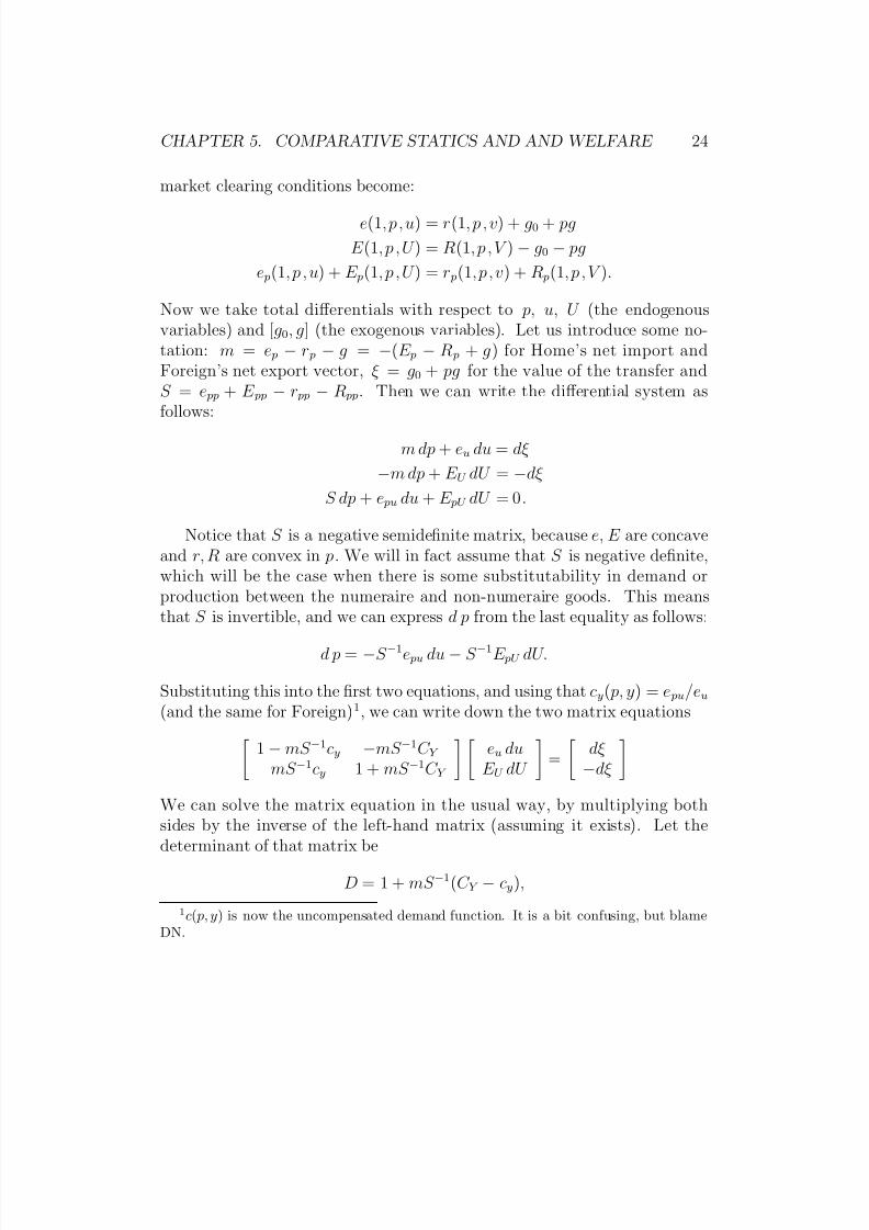
market clearing conditions become:
e(1,p ,u) = r(1, p , v) + g0 + pg
E (1, p , U ) = R(1, p , V ) − g0 − pg
e p(1, p , u) + E p(1, p , U ) = r p(1,p ,v) + R p(1, p , V ).
Now we take total differentials with respect to p, u, U (the endogenousvariables) and [g0, g] (the exogenous variables). Let us introduce some no-tation: m = e p − r p − g = −(E p − R p + g) for Home’s net import andForeign’s net export vector, ξ = g0 + pg for the value of the transfer andS = e pp + E pp − r pp − R pp. Then we can write the differential system asfollows:
m dp + eu du = dξ
−m dp + E U dU = −dξ
S dp + e pu du + E pU dU = 0.
Notice that S is a negative semidefinite matrix, because e, E are concaveand r, R are convex in p. We will in fact assume that S is negative definite,which will be the case when there is some substitutability in demand orproduction between the numeraire and non-numeraire goods. This meansthat S is invertible, and we can express d p from the last equality as follows:
d p = −S −1e pu du − S −1E pU dU.
Substituting this into the first two equations, and using that cy( p, y) = e pu/eu
(and the same for Foreign)1, we can write down the two matrix equations 1 − mS −1cy −mS −1C Y
mS −1cy 1 + mS −1C Y
eu duE U dU
=
dξ −dξ
We can solve the matrix equation in the usual way, by multiplying bothsides by the inverse of the left-hand matrix (assuming it exists). Let thedeterminant of that matrix be
D = 1 + mS −1(C Y − cy),
1c( p, y) is now the uncompensated demand function. It is a bit confusing, but blameDN.
8/20/2019 Konya I. Lectures Notes in International Trade (Boston, 2001)(118s)_GI
http://slidepdf.com/reader/full/konya-i-lectures-notes-in-international-trade-boston-2001118sgi 33/118
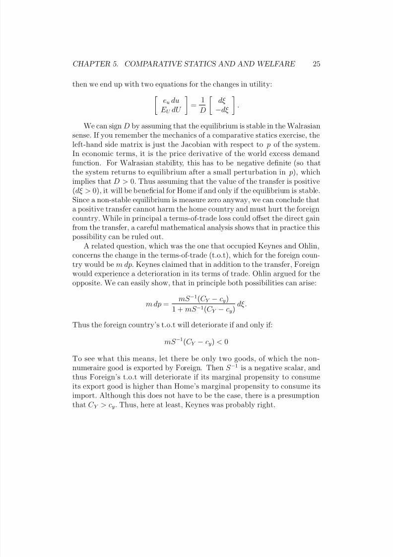
CHAPTER 5. COMPARATIVE STATICS AND AND WELFARE 25
then we end up with two equations for the changes in utility: eu duE U dU
=
1D
dξ −dξ
.
We can sign D by assuming that the equilibrium is stable in the Walrasiansense. If you remember the mechanics of a comparative statics exercise, theleft-hand side matrix is just the Jacobian with respect to p of the system.In economic terms, it is the price derivative of the world excess demandfunction. For Walrasian stability, this has to be negative definite (so thatthe system returns to equilibrium after a small perturbation in p), whichimplies that D > 0. Thus assuming that the value of the transfer is positive(dξ > 0), it will be beneficial for Home if and only if the equilibrium is stable.Since a non-stable equilibrium is measure zero anyway, we can conclude thata positive transfer cannot harm the home country and must hurt the foreigncountry. While in principal a terms-of-trade loss could offset the direct gainfrom the transfer, a careful mathematical analysis shows that in practice thispossibility can be ruled out.
A related question, which was the one that occupied Keynes and Ohlin,concerns the change in the terms-of-trade (t.o.t), which for the foreign coun-try would be m dp. Keynes claimed that in addition to the transfer, Foreignwould experience a deterioration in its terms of trade. Ohlin argued for theopposite. We can easily show, that in principle both possibilities can arise:
m dp = mS −1(C Y − cy)
1 + mS −1(C Y − cy) dξ.
Thus the foreign country’s t.o.t will deteriorate if and only if:
mS −1(C Y − cy) < 0
To see what this means, let there be only two goods, of which the non-numeraire good is exported by Foreign. Then S −1 is a negative scalar, andthus Foreign’s t.o.t will deteriorate if its marginal propensity to consume
its export good is higher than Home’s marginal propensity to consume itsimport. Although this does not have to be the case, there is a presumptionthat C Y > cy. Thus, here at least, Keynes was probably right.
8/20/2019 Konya I. Lectures Notes in International Trade (Boston, 2001)(118s)_GI
http://slidepdf.com/reader/full/konya-i-lectures-notes-in-international-trade-boston-2001118sgi 34/118
CHAPTER 5. COMPARATIVE STATICS AND AND WELFARE 26
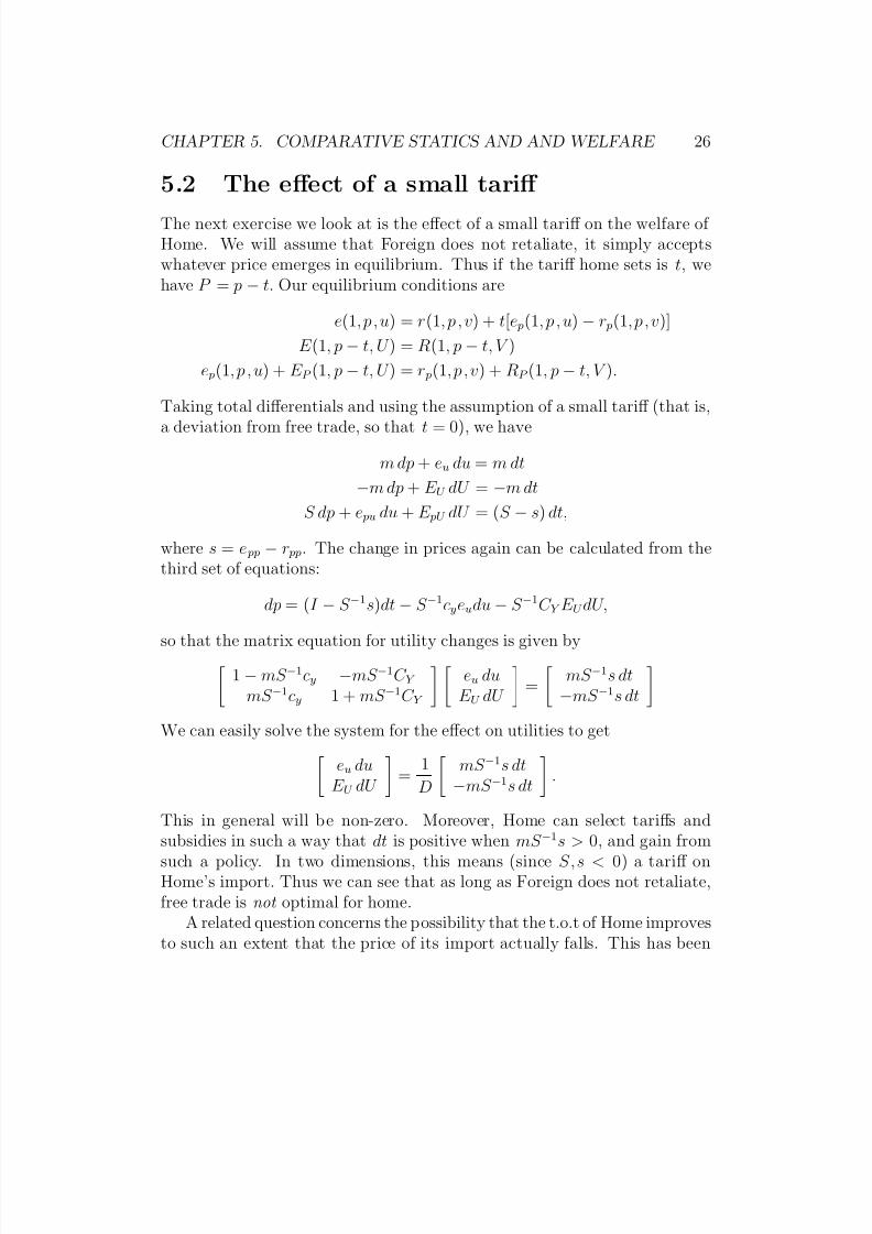
5.2 The effect of a small tariff
The next exercise we look at is the effect of a small tariff on the welfare of Home. We will assume that Foreign does not retaliate, it simply acceptswhatever price emerges in equilibrium. Thus if the tariff home sets is t, wehave P = p − t. Our equilibrium conditions are
e(1,p ,u) = r(1, p , v) + t[e p(1, p , u) − r p(1,p ,v)]
E (1, p − t, U ) = R(1, p − t, V )
e p(1, p , u) + E P (1, p − t, U ) = r p(1,p ,v) + RP (1, p − t, V ).
Taking total differentials and using the assumption of a small tariff (that is,
a deviation from free trade, so that t = 0), we have
m dp + eu du = m dt
−m dp + E U dU = −m dt
S dp + e pu du + E pU dU = (S − s) dt,
where s = e pp − r pp. The change in prices again can be calculated from thethird set of equations:
dp = (I − S −1s)dt − S −1cyeudu − S −1C Y E U dU,
so that the matrix equation for utility changes is given by 1 − mS −1cy −mS −1C Y
mS −1cy 1 + mS −1C Y
eu duE U dU
=
mS −1s dt−mS −1s dt
We can easily solve the system for the effect on utilities to get eu duE U dU
=
1
D
mS −1s dt−mS −1s dt
.
This in general will be non-zero. Moreover, Home can select tariffs andsubsidies in such a way that dt is positive when mS −1s > 0, and gain from
such a policy. In two dimensions, this means (since S,s < 0) a tariff onHome’s import. Thus we can see that as long as Foreign does not retaliate,free trade is not optimal for home.
A related question concerns the possibility that the t.o.t of Home improvesto such an extent that the price of its import actually falls. This has been

8/20/2019 Konya I. Lectures Notes in International Trade (Boston, 2001)(118s)_GI
http://slidepdf.com/reader/full/konya-i-lectures-notes-in-international-trade-boston-2001118sgi 35/118
8/20/2019 Konya I. Lectures Notes in International Trade (Boston, 2001)(118s)_GI
http://slidepdf.com/reader/full/konya-i-lectures-notes-in-international-trade-boston-2001118sgi 36/118
CHAPTER 5. COMPARATIVE STATICS AND AND WELFARE 28
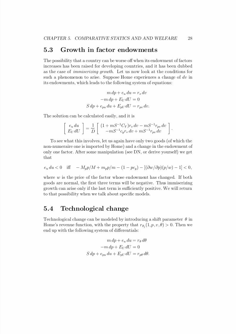
5.3 Growth in factor endowments
The possibility that a country can be worse off when its endowment of factorsincreases has been raised for developing countries, and it has been dubbedas the case of immiserizing growth . Let us now look at the conditions forsuch a phenomenon to arise. Suppose Home experiences a change of dv inits endowments, which leads to the following system of equations:
m dp + eu du = rv dv
−m dp + E U dU = 0
S dp + e pu du + E pU dU = r pv dv.
The solution can be calculated easily, and it is eu duE U dU
=
1
D
(1 + mS −1C Y )rv dv − mS −1r pv dv
−mS −1cyrv dv + mS −1r pv dv
.
To see what this involves, let us again have only two goods (of which thenon-numeraire one is imported by Home) and a change in the endowment of only one factor. After some manipulation (see DN, or derive yourself) we getthat
eu du < 0 iff − M p p/M + m p p/m − (1 − pcy) − [(∂w/∂p)( p/w) − 1] < 0,
where w is the price of the factor whose endowment has changed. If bothgoods are normal, the first three terms will be negative. Thus immiserizinggrowth can arise only if the last term is sufficiently positive. We will returnto that possibility when we talk about specific models.
5.4 Technological change
Technological change can be modeled by introducing a shift parameter θ inHome’s revenue function, with the property that rθj(1,p ,v ,θ) > 0. Then weend up with the following system of differentials:
m dp + eu du = rθ dθ
−m dp + E U dU = 0
S dp + e pu du + E pU dU = r pθ dθ.
8/20/2019 Konya I. Lectures Notes in International Trade (Boston, 2001)(118s)_GI
http://slidepdf.com/reader/full/konya-i-lectures-notes-in-international-trade-boston-2001118sgi 37/118
CHAPTER 5. COMPARATIVE STATICS AND AND WELFARE 29
This can be solved easily to yield eu duE U dU
=
1D
(1 + mS −1C Y )rθ dθ − mS −1r pθ dθ
−mS −1cyrθ dθ + mS −1r pθ dθ
.
A special case is when θ is the TFP parameter, so that x j = θ jf j(v j).We can show from the alternative definition of the revenue function that inthis case r( p, v, θ) = r(θp,v), and therefore rθ = px, r pθ = x. Assuming twogoods and technological progress only in the non-numeraire good, we havethat
eu duE U dU
=
1
D
[ px − mx(1 − pC Y ))/S ] dθ
mx(1 − pcy)/S dθ
.
If both goods are normal, 0 < pcy < 1. Thus Foreign will benefit from atechnological change in Home if and only if it imports the good in which thechange occurred. In other words, Foreign will benefit from growth in Home’sexport sector and loose from growth in Home’s import competing sector.Since the world has to benefit from growth (eu du + E U dU = rθ dθ = pxdθ),Home will benefit in the latter case. When the change occurs in Home’sexport sector, it will loose if the t.o.t loss (the second term) is greater thanthe direct gain ( px). You can work out the condition for that, but it is notvery illuminating.

8/20/2019 Konya I. Lectures Notes in International Trade (Boston, 2001)(118s)_GI
http://slidepdf.com/reader/full/konya-i-lectures-notes-in-international-trade-boston-2001118sgi 38/118
Chapter 6
Simple trade models
Here we will look at special cases of the general trade model we developedearlier. The main simplification will be to limit the number of goods and fac-tors, which lead to very sharp – if highly model specific – conclusions. Muchof international trade was taught in terms of these simple models, mostly theHecksher-Ohlin variety. They do indeed yield many useful insights, but youhave to bear in mind their limitations. Now that we have seen the generalmodel, we are better equipped to decide just how special the assumptionsare and what features of the results survive.
6.1 The Heckscher-Ohlin model – the role of factor endowments
There are two goods produced by two factors. We will assume that in equi-librium both goods are produced, which gives us two conditions for factormarket clearing and two for zero profits. Let a(w) be the matrix of unit inputcoefficients, than we have
a(w)x = v
andwa(w) = p.
The first result we note is the Factor Price Equalization Theorem , whichrequires that both countries produce the two goods in equilibrium. We havealready seen that this is a restriction on factor endowments, so we do nothave to assume no specialization separately. This shows the advantage of
30
8/20/2019 Konya I. Lectures Notes in International Trade (Boston, 2001)(118s)_GI
http://slidepdf.com/reader/full/konya-i-lectures-notes-in-international-trade-boston-2001118sgi 39/118
CHAPTER 6. SIMPLE TRADE MODELS 31
the integrated equilibrium approach, since we traced back FPE to model
fundamentals. We also saw that in the 2x2 case FPE has positive measure.The next result is the Rybczynski Theorem , which gives the connectionbetween factor endowments and output levels, given unchanging commodity(and hence factor) prices. With constant output (and factor) prices, x is alinear function of endowments, and we can calculate the change in productionlevels easily. Let us introduce the “hat” notation for percentage changes, sothat for any variable y we have y = dy/y. Taking logs of the factor marketclearing conditions and using λij = aijx j/vi for the share of factor i used insector j , we have
v1 = λ11x1 + λ12x2
v2 = λ21x1 + λ22x2.
We can solve for the percentage changes in production to get
x1 = λ22v1 − λ12v2λ11λ22 − λ12λ21
x2 = λ11v2 − λ21v1λ11λ22 − λ12λ21
.
It is easy to show the the denominator is proportional to the difference inrelative factor intensities (λ11λ22−λ12λ21 = x1x2
v1v2[a11a22−a12a21]), so without
loss of generality we can assume that it is positive. In words, we assume thatgood 1 is more intensive in the use of factor 1 for the given factor prices.Then it is easy to show that1
v1 > v2 ⇒ x1 > v1 > v2 > x2,
which is Jones’s famous magnification result. It says that changes in factorendowments show up magnified in production. A special case is the Ry-bczynski Theorem, when only one factor endowment changes. If, say, v2 = 0,we have
x1 > v1 > 0 > x2.
Thus the percentage change in the production of good 1 (that uses factor 1intensively) is bigger than the percentage change in the endowment of factor1, and the production of good 2 falls.
1Do it, using the fact that λi1 + λi2 = 1.
8/20/2019 Konya I. Lectures Notes in International Trade (Boston, 2001)(118s)_GI
http://slidepdf.com/reader/full/konya-i-lectures-notes-in-international-trade-boston-2001118sgi 40/118
8/20/2019 Konya I. Lectures Notes in International Trade (Boston, 2001)(118s)_GI
http://slidepdf.com/reader/full/konya-i-lectures-notes-in-international-trade-boston-2001118sgi 41/118
CHAPTER 6. SIMPLE TRADE MODELS 33
to export good 1 and vice versa. Notice that it is the same argument that
we made with fixed coefficients at the first lecture, and it holds for variablecoefficients as long as FPE prevails.
6.2 The generalized Ricardian model – the
role of technology
We saw the simple Ricardian model at the beginning of the class. Oneproblem with the two-good/one factor setting is that the revenue functionis not differentiable in a non-trivial subset of the parameter values. To seethis, note that r can be written as (normalizing the price of good 1)
r( p, v) = max
v
a1, pv
a2
.
This function has a kink at p = a2/a1, which means that r is not differen-tiable there. Although such a relative price might seem exceptional, it canin fact result in a trade equilibrium with positive measure. This means thatcomparative statics is difficult, since one cannot use the standard tools.
To remedy this, we will use the continuum good extension of the Ricardianmodel, developed by Dornbusch, Fischer and Samuelson. It turns out to besurprisingly simple, and very suitable to analyze the effects of technology.
Suppose there is one factor, labor, and a continuum of goods indexed byz ∈ [0, 1]. The unit labor coefficient is a(z ) for good z in the home countryand a∗(z ) for the foreign country and we define
A(z ) = a∗(z )
a(z ) .
Without loss of generality, we arrange goods in such a way that A(z ) < 0,i.e. the home country is relatively more efficient in the production of goodswith low index. The home country will produce good z if it will have a costadvantage in it, that is, if
ω < A(z ),
where ω = w/w∗ (Home’s wage rate relative to Foreign). Given our assump-tion on A(z ), Home will produce goods 0 ≤ z ≤ ζ (ω), where ζ (ω) = A−1(ω)and hence ζ (ω) < 0. By the same argument Foreign will specialize in theproduction of all the other goods, ζ ≤ z ≤ 1.
8/20/2019 Konya I. Lectures Notes in International Trade (Boston, 2001)(118s)_GI
http://slidepdf.com/reader/full/konya-i-lectures-notes-in-international-trade-boston-2001118sgi 42/118
CHAPTER 6. SIMPLE TRADE MODELS 34
On the demand side we will use the generalized Cobb-Douglas prefer-
ences
2
, which imply that expenditure share of each good is constant. Inparticular, we will have p(z )c(z )
Y = b(z )
for both countries. Let us define the fraction of world expenditure spent onHome goods as
ν (ζ ) =
ζ 0
b(z ) dz,
with the property thatν (ζ ) = b(ζ ) > 0.
In equilibrium, given full specialization, national income in Home mustequal spending on Home goods. Let us normalize the world population to1 and let L be the population of Home. Then the following equilibriumcondition must hold:
wL = ν (ζ )[wL + w∗(1 − L)],
from which we get that
ω = ν (ζ )
1 − ν (ζ )
1 − L
L .
It is easy to check that the right-hand side is increasing in ζ .
We now close the model with the reduced-form equilibrium condition thatdetermines ζ :
A(ζ ) = ν (ζ )
1 − ν (ζ )
1 − L
L .
Since the left-hand side decreases and the right-hand side increases with ζ , theequilibrium is unique and stable. From the knowledge of the cutoff good wecan solve for all the other variables, notably for ω and the commodity prices
p(z ) = min{a(z )w, a∗(z )w∗}. Before we move to comparative statics, let usnote that the relative wage ω is a measure of well-being in both countries.Indirect utility in Home is given by
v =
ζ 0
b(z )log[b(z )/a(z )] dz +
1ζ
b(z )log[b(z )ω/a∗(z )] dz,
2The utility function is given by u = 1
0 b(z)log c(z) dz, with
1
0 b(z) dz = 1.
8/20/2019 Konya I. Lectures Notes in International Trade (Boston, 2001)(118s)_GI
http://slidepdf.com/reader/full/konya-i-lectures-notes-in-international-trade-boston-2001118sgi 43/118
CHAPTER 6. SIMPLE TRADE MODELS 35
which is increasing in ω3. You can derive the similar expression for Foreign
to show that it decreases with ω .An obvious comparative statics result concerns L, the relative size of the home country. An increase in L will lead to an increase in ζ , whichmeans that the relative wage ω goes down. Thus Home utility will decreaseand Foreign utility will increase. The reason is an unfavorable shift in theterms-of-trade for Home, which results from the fact that at an unchangedrelative wage Home supply increases, but world demand does not change.Thus to eliminate the inequilibrium ω must decrease, which will lead to anincreased demand for Home goods and to an increased range of goods producethere. Notice that although Foreign “lost” some marginal goods to Home,it is nevertheless better off with the change. In this model, small is indeed
beautiful!The next change we consider is in technology. In particular, let us assume
that Foreign unit labor requirement is λa∗(z ) for any z , and there is a decreasein the parameter λ. Our task is a bit complicated now, since indirect utilitynow depends directly on λ. To see more clearly, let us still use the notationA(ζ ) = a∗(ζ )/a(ζ ), and let B(ζ ) = ν (ζ )/[1 − ν (ζ )]. Using the equilibriumcondition and the “hat” notation, we can easily show that
ζ =λ
B −
A
,
where i is the elasticity of the particular function, and we know that A < 0and
B > 0. We also have that
ω = λ + A
ζ =
B
B −
A
λ,
which means that λ < ω < 0. Thus an improvement in Foreign’s technologywill lead to a lower relative wage in Home, but the percentage decrease willbe smaller than the percentage drop in λ. This means that Foreign will gainboth because of increased efficiency and a higher relative wage. Home willalso gain, because its relative wage decreases by less than the increase in
foreign efficiency, and thus its purchasing power in terms of foreign goodsincreases (whereas it does not change in its own goods).
3Note that v depends on ω indirectly through ζ , but that indirect derivative will bezero, since vζ = 0.

8/20/2019 Konya I. Lectures Notes in International Trade (Boston, 2001)(118s)_GI
http://slidepdf.com/reader/full/konya-i-lectures-notes-in-international-trade-boston-2001118sgi 44/118
CHAPTER 6. SIMPLE TRADE MODELS 36
A final change we study is a convergence in technology between Home and
Foreign. Suppose initially Home had the higher wage rate, that is ω > 1. Wecompare this with complete convergence, when ω = A(z ) ≡ 1. We can showthat such a change results in a loss for Home and in a gain for Foreign. Noticethat when technologies are the same, there is no reason to trade. This meansthat the real wage in Home in terms of any good is given by 1/a(z ). On theother hand, when Foreign had an inferior tecnology, real wage in terms of animported good was ω/a∗(z ) > 1/a(z ) (since it was more efficient to producethe good in Foreign) and real wage in terms of an exported good was 1 /a(z ).Thus Home’s real wage was higher in the original situation. Foreign, on theother hand, enjoys the productivity gain for goods produced there and theterms-of-trade gain which is just the opposite of Home’s loss. The reason
for such stark result is that such a convergence must be biased towards theimport competing sector in Foreign, since it had a larger technological gapin those goods (almost by definition). And as we saw earlier, a growth in theimport competing sector must hurt the other country.
6.3 The specific factors model – income dis-
tribution
The specific factor model can be thought of as another attempt to make theRicardian model suitable for comparative statics, since labor has a decreasingmarginal product in each use. The most plausible reason for this is theexistence for another factor that is “specific” to a sector and is immobilebetween different uses. One can think of buildings and machinery that cannotbe converted for use in a different industry. Thus we will assume the existenceof two sectors and three factors. One (labor) is mobile between the sectors,but the other two are not. The endowments of the factors in the Homecountry are L, K 1 and K 2, respectively.
On the production side we have various conditions. Let F i(Li, K i) be theproduction function in sector i, which we can also write as K iF i(Li/K i, 1) =K if i(li). We assume the standard properties and the Inada conditions for F i,
which means that f i is increasing and concave in li and limli=0 f i(li) = ∞.
Let w be the wage rate and πi be the return to specific factor i. From profitmaximization we have that
p1f 1(l1) = w = p2f 2(l2),
8/20/2019 Konya I. Lectures Notes in International Trade (Boston, 2001)(118s)_GI
http://slidepdf.com/reader/full/konya-i-lectures-notes-in-international-trade-boston-2001118sgi 45/118
CHAPTER 6. SIMPLE TRADE MODELS 37
andπi
pi = [f i(li) − lif
i(li)].An important result for future reference is that
πi
pi
(li) = −lif i (li) > 0
The factor market clearing condition is simply K 1l1 + K 2l2 = L. We will usethe model to look at changes in the factor returns in response to a change inL, K i and the relative price. For the latter we normalize the price of good 1and write p = p2/p1.
Let us start with a change in p. We can see that there must be a re-
allocation of labor from sector 1 to sector 2, which leads to an increase inw and to a decrease in w/p (since marginal value products equalize in thetwo sectors). We can also see that π1 must fall, because it is an increasingfunction of l1. On the other hand, π2/p must rise, since it is an increasingfunction of l2. Thus real wage rises in terms of one good and falls in terms of the other, whereas the return of specific factor 1 (2) decreases (increases) interms of both goods. It is also apparent that the output of good 1 increasesand the output of good 2 decreases. If the price increase comes from a tariff,we have the intuitive result that capitalists in the protected sector will bebetter off (except, of course, when Metzler’s paradox arises).
Now let us take a look at a change in the endowment of the mobile factor,L. To accommodate the extra labor, the marginal value product of labormust fall in both sectors, so that w falls. On the other hand, both l1 andl2 will rise, so the returns to both specific factors must increase. Thus laboris unambiguously hurt and the specific factors are unambiguously better off with the change. When the amount of a specific factor changes (say in sector1), the marginal product of labor there rises. To restore equilibrium, laborhas to flow into sector 1. Suppose that this process continues until the originallabor/capital ratio l1 is restored. But since l2 have fallen, the value marginalproducts are not equalized across sectors. Thus l1 will also decrease, andthe wage rate will rise. This implies that πi must fall for i = 1, 2. Thus
an increase in the endowment of a specific factor benefits the owners of themobile factor, and hurts the owners of both specific factors.
Before we finish, let us look at the output changes in the various cases.When p increases, production in sector 1 increases and production in sector2 falls, but by a smaller proportion than the change in p. If L rises, both

8/20/2019 Konya I. Lectures Notes in International Trade (Boston, 2001)(118s)_GI
http://slidepdf.com/reader/full/konya-i-lectures-notes-in-international-trade-boston-2001118sgi 46/118
CHAPTER 6. SIMPLE TRADE MODELS 38
outputs increase, but by less than L. Finally, an increase in a specific factor
endowment leads to a smaller proportional increase in the production of thatsector and a fall in the production of the other sector. Thus the magnificationresult we saw in the Heckscher-Ohlin model does not arise here.

8/20/2019 Konya I. Lectures Notes in International Trade (Boston, 2001)(118s)_GI
http://slidepdf.com/reader/full/konya-i-lectures-notes-in-international-trade-boston-2001118sgi 47/118
Chapter 7
Empirical strategies
Im the notes I do not want to discuss specific results from various papers, youare referred for those to Feenstra, Helpman (1998) and Harrigan (2001). Thelatter two are survey articles that cite many original papers and summarizetheir results. Instead, I will focus on the empirical strategies researchers haveused to test the theory of comparative advantage. As a first note, let me quoteHarrigan by saying that almost no empirical work has tested the doctrine of comparative advantage directly. This is, to some extent, inevitable, since werarely (if ever) observe autarchy prices together with net trade vectors. Thereare natural experiments that can be used, one notable example is Japan 150years ago (Bernhofen and Brown, see Feenstra).
This means that empirical work usually tests not comparative advantage,but explanations for it. Various restrictions are made in order to get rela-tionships between measurable variables. By far the most common model tobe tested is the Heckscher-Ohlin model, and its various generalizations. Atits most restrictive form, it assumes two goods and factors, identical tech-nologies and identical homothetic preferences to predict trade patterns. Amore general result links factor endowments and the factor content of trade,as long as we assume FPE. Since recent work focuses on the Vanek equation,let us thus first look at the testable implications with FPE and then see whatpossibilities and problems arise without it.
39

8/20/2019 Konya I. Lectures Notes in International Trade (Boston, 2001)(118s)_GI
http://slidepdf.com/reader/full/konya-i-lectures-notes-in-international-trade-boston-2001118sgi 48/118
CHAPTER 7. EMPIRICAL STRATEGIES 40
7.1 The basic equation
We saw earlier that in the case of identical technologies, identical homotheticpreferences and FPE the factor content of trade is uniquely determined byendowments. In particular, we have
tkv = skv − vk,
with the previously introduced notation. This is an equation in which we canmeasure all variables (there are no parameters to estimate), so we cannot useregression analysis to test it. Instead, one can compute a rank-correlationmeasure for the left- and right-hand sides. Alternatively, we can checkwhether the sign of the two sides coincides. Although these are fairly weaktests, the evidence is not very supportive (see Bowen-Leamer-Sveikauskas).
In particular, there are three ways how the data fails to support the basicfactor abundance hypotheses (see Trefler 1993, 1995). These are:
• The measures of factor content are compressed towards zero.
• Poor countries have systematically larger values of tkv . For rich countries
the opposite is true.
• Poor countries tend to be abundant in more factors than rich countries.
Let us see what people have tried to do to recouncile the model with theseempirical failures.
7.2 Extensions with FPE
One way to extend the previous equation is by allowing differences in tech-nology. If these are factor augmenting, countries with different technologiesthat have the same amount physical units of a factor can have different en-dowments in efficiency units . Then FPE refers not to the price of physical,but of efficiency units and we can use the Vanek argument, as long as en-
dowments are not too far away. The problem in this case, however, is thatwe only observe physical units. To see why this is a problem, for each factorwrite endowments in efficiency units as πk
i vki , where πk
i is the technology co-efficient for factor i in country k relative to some benchmark country. Then
8/20/2019 Konya I. Lectures Notes in International Trade (Boston, 2001)(118s)_GI
http://slidepdf.com/reader/full/konya-i-lectures-notes-in-international-trade-boston-2001118sgi 49/118
CHAPTER 7. EMPIRICAL STRATEGIES 41
the factor content of trade for factor i can be written as
tkvi = sk
l
πliv
li − πk
i vki .
The problem is that we do not know the coefficients πki , and we do not
have degrees of freedom to estimate them. There is a different technologyparameter for each country-factor pair, and this is the number of equations wehave. This means that πk
i can be calculated as a residual, and we can alwaysexplain the pattern of trade with the calculated technological differences.
Of course the calculated technology parameters have to be “plausible”.If, for example, Albanian technology parameters would come out consistentlygreater than German ones, we would be suspect our results. Still, we needsome benchmark to which we measure the plausibility of the parameters.One possibility is to assume that πk
i = πk, that is technology is country, butnot factor specific. Then if country 1 is the benchmark country, we can easilyshow that πk = wk
i /w1i for any i, and we can use the observable factor price
ratios as measures of technology parameters. Alternatively, we can assumethat there exist groups of countries, such that within a group all countriesshare the same technology, but technology is different across groups. Anobvious example to such a group is the OECD, another could be NICs, whilea third group could be LDCs. With this restriction we gain degrees of freedomto estimate the π ’s and see if they lead to plausible numbers.
To conclude, in the presence of FPE we can test the factor abundanceusing the Vanek result for the factor content of trade, preferably augmentedby some restricted form of technological differences. One can also relax theassumption of identical homothetic preferences and allow for home bias inconsumption, although in the classical theory of trade there is no really goodreason why such bias would occur. The results in Helpman or Harrigan showthat such an augmented model performs reasonably well, but some importantproblems remain.
7.3 Results without FPE
There is some independent evidence that FPE does not hold in many cases.The efficiency unit argument is a nice way to introduce technological differ-ences, but it also makes FPE less likely. Remember that for FPE we need
8/20/2019 Konya I. Lectures Notes in International Trade (Boston, 2001)(118s)_GI
http://slidepdf.com/reader/full/konya-i-lectures-notes-in-international-trade-boston-2001118sgi 50/118
CHAPTER 7. EMPIRICAL STRATEGIES 42
that factor endowments are not very different across countries. This is es-
pecially hard for labor endowments, which might be similar in the physicalsense but very different if interpreted as human capital. Thus we need toinvestigate the implications of a failure of FPE.
The main problem with estimating the factor content of trade when FPEdoes not hold is that techniques of production differ across countries in away that cannot be fixed by introducing efficiency units. Even with identicaltechnologies, different factor prices lead to different input vectors, as weindicated it when we wrote the unit input coefficient matrix as a(w). In hisfamous work leading to the Leontief-paradox 1, Leontief used US input-outputcoefficients to measure the factor content of US trade. This is only correctwhen there is FPE, otherwise foreign technology will not be the same and
the calculated factor content will be biased.An illustration of the problem can be found in Helpman. Suppose that
there are two goods, two countries and two factors but no FPE. Let countryA have a higher capital-labor ratio, and hence a higher wage rate and alower rental rate on capital. Then we know that aA
Ki > aBKi and aA
Li < aBLi
for i = 1, 2. Let good 2 be the more capital intensive, and suppose thatboth countries specialize, country A in good 2 and country B good 1. Givenidentical homothetic preferences, the net import vector of country A is givenby
mA = sAxB
1
−sBxA
2 .
If we use A’s technology matrix to calculate the factor content of its netimport vector, we get
tAv =
sAaA
K 1xB1 − sBaA
K 2xA2
sAaAL1xB
1 − sBaAL2xA
2
=
aA
K1
aBK1
sAK B − sBK A
aAL1
aBL1
sALB − sBLA
.
On the other hand,
sAv − vA = sA(K A + K B) − K A
sA(LA + LB)−
LA = sAK B − sBK A
sALB
−sBLA
1Leontief tried to measure the factor content of US trade after WWII. His resultsindicated that the US is a net exporter of labor and an importer of capital. Since atthat time the US had the most advanced economy, Leontief considered his results asparadoxical.
8/20/2019 Konya I. Lectures Notes in International Trade (Boston, 2001)(118s)_GI
http://slidepdf.com/reader/full/konya-i-lectures-notes-in-international-trade-boston-2001118sgi 51/118
CHAPTER 7. EMPIRICAL STRATEGIES 43
gives the “real” factor content of trade measured by the differences in factor
endowments.Thus the factor content of A’s net import vector will be compressed to-wards zero when A’s technology is used. This can explain the first empiricalregularity called missing trade , because measured factor content will be bi-ased downward. The reason for this is that when we use A’s techniques tocalculate imports from B, we understate the amount of labor and overstatethe amount of capital used in producing good 1. To get the correct measure,we need to use the techniques for the exporter for any good.
It is possible to get a weak, but testable restriction on the pattern of bilateral trade without FPE. Assume still that technology is the same in thetwo countries, that is, the revenue function has the same form. Let xk be
the production vector of country k and tkl be the factor content of importsfrom country l to k using the exporter’s techniques a(wl). The main insightis that given the factor endowment vk + tkl, the production vector xk + mkl
would be feasible. It is not necessarily optimal, however, since exploiting itsdiffering factor prices country k can use different techniques to achieve higherrevenue:
p(xk + mkl) ≤ r( p, vk + tkl)
≤ r( p, vk) + rv( p, vk)tkl
= pxk + wktkl,
where the second inequality follows from the concavity of r in v. Comparingthe first and the last lines yields pmkl ≤ wktkl. In the exporting country, onthe other hand, the value of exports equals the payment of the factors usedin producing them, therefore pmkl = wltkl. Combining these two yields
(wk − wl)tkl ≥ 0.
Repeating the exercise for country l using the techniques of country k, wealso get that
(wl − wk)tlk ≥ 0,
and that(wk − wl)(tkl − tlk) ≥ 0.
These inequalities imply that a country will on average export a factor whoseprice is relatively lower there. They are weak in a sense that they only predict

8/20/2019 Konya I. Lectures Notes in International Trade (Boston, 2001)(118s)_GI
http://slidepdf.com/reader/full/konya-i-lectures-notes-in-international-trade-boston-2001118sgi 52/118
CHAPTER 7. EMPIRICAL STRATEGIES 44
correlations, but this is all we can hope as a general result. You can check that
in the case of two factors the correlation actually becomes a clear prediction,but just as with many results this does not generalize.
8/20/2019 Konya I. Lectures Notes in International Trade (Boston, 2001)(118s)_GI
http://slidepdf.com/reader/full/konya-i-lectures-notes-in-international-trade-boston-2001118sgi 53/118
Part II
Increasing returns and the
“New Trade Theory”
45
8/20/2019 Konya I. Lectures Notes in International Trade (Boston, 2001)(118s)_GI
http://slidepdf.com/reader/full/konya-i-lectures-notes-in-international-trade-boston-2001118sgi 54/118
46
The “New Trade Theory” is not so new now, since it originated around
1980 and was developed pretty much by the middle of that decade. Themain reasons for its emergence were both theoretical and empirical. On thetheoretical side, there was a long tradition in trade theory that emphasizedincreasing returns and specialization as causes of trade, but economists couldnot handle imperfect competition – that is a natural consequence of increas-ing returns – very well until the late 1970’s. With advances in game theoryand industrial organization, the necessary modeling tools to analyze imper-fect competition were available. On the empirical front, it was observedthat much of trade is in varieties of similar goods, which is known as “intra-industry” trade. Also, most of world trade are between seemingly similarnations, that is the within OECD. The theory of comparative advantage, on
the other hand, predicts that trade should be greatest between countries whohave very different endowments.
Thus theorists started to think about models of increasing returns andimperfect competition. As folk wisdom says, however, there are many waysto be imperfectly competitive, and as of today there is no generally acceptedway to model market power. Thus attention turned to specific models thathighlight one particular aspect of reality, in the hope that a few of thesesimple models would give us enough intuition about the general issues in-volved. We will study three types of such models: increasing returns due toexternalities, oligopolic markets and monopolistic competition. Let us startwith the first.
8/20/2019 Konya I. Lectures Notes in International Trade (Boston, 2001)(118s)_GI
http://slidepdf.com/reader/full/konya-i-lectures-notes-in-international-trade-boston-2001118sgi 55/118
Chapter 8
External economies of scale
This approach has the longest tradition to model increasing returns. Strictlyspeaking it does not quite fit into the “New Trade Theory“, because it avoidsthe question of market structure. The attraction of externalities is that firmsstill perceive themselves as price takers, and hence perfect competition ispreserved. This modeling technique is somewhat out of fashion, but it stilldeserves some mention partly because of its earlier popularity and partlybecause it is still the best way to study some important issues.
8.1 Gains from trade
We will start with describing the autarchy and trade equilibria and we willtake a look at the possible gains from trade. To simplify a bit, we do notallow for joint production, thus production of each good can be described bya production function:
x j = f j(v j, ξ ).
The notation is as before, and ξ is the vector of external effects. Examplesinclude overall production in the sector, or the average level of human cap-ital in the country, or world population. There are two issues that will beimportant: first, externalities can be local or global in scope, and second, the
variables that affect the production function might be different in free tradethan in autarchy. We will return to these issues later.Since perfect competition still applies, we can represent the total value
of production by the revenue function, just as before. Now it can be defined
47

8/20/2019 Konya I. Lectures Notes in International Trade (Boston, 2001)(118s)_GI
http://slidepdf.com/reader/full/konya-i-lectures-notes-in-international-trade-boston-2001118sgi 56/118
CHAPTER 8. EXTERNAL ECONOMIES OF SCALE 48
as follows:
r( p, v, ξ ) = maxx
j
p jf j(v j, ξ )| j
v j ≤ v
.
Given the consumption side, the equilibrium in autarchy and free trade canbe defined exactly as before. The only difference is that ξ must be consistentwith equilibrium. If, say, ξ is the vector (0, 0,...,x j,..., 0) for industry j, thenthe x j in ξ must equal actual production.
An important question concerns the gains of trade. It is no longer truethat a country necessarily gains from trade, and we will see an example forthe opposite. For now we give a sufficient condition for positive gains,whichalso reveals the extra channel that operates now. The sufficient condition is
j
p jf j(v ja , ξ ) ≥ j
p jf j(v ja, ξ a),
where v ja is the factor input vector in industry j in autarchy. To see that thecondition is sufficient, we show that with it the autarchy production (andconsumption) vector is affordable at free trade:
pxa ≤ j
p jf j(v ja, ξ ) (from our condition)
≤ j
p jf j(v j, ξ ) (v ja is feasible)
= r( p, v, ξ ).
The condition states that productivity is greater at the free trade valueof the external effects than at the autarchy value. It reveals an additionalsource of gain in trade, which can either come from larger scale or exposure toforeign external economies. Note that even if the condition does not hold, thecountry can gains from trade through the traditional channels (a possibilityto trade at a price different from the autarchy one). Thus trade is harmfulonly if the loss due to less favorable externalities outweigh the static efficiencygains. Let us see an example that illustrates these possibilities.
8.2 An example
Let us take a simple Ricardian model with two goods and two countries. Wechoose units in such a way that the unit labor requirement is one in both

8/20/2019 Konya I. Lectures Notes in International Trade (Boston, 2001)(118s)_GI
http://slidepdf.com/reader/full/konya-i-lectures-notes-in-international-trade-boston-2001118sgi 57/118
CHAPTER 8. EXTERNAL ECONOMIES OF SCALE 49
sectors. Productivity in sector 1 also depends on aggregate production there,
so that the production functions can be written asx1 = x
1/21 L1
x2 = L2,
where x1 is aggregate production in sector 1. Preferences take the Cobb-Douglas form, with an α < 1/2 fraction of consumer spending falling ongood 1. We assume that technology and tastes are the same for the twocountries.
There is a unique autarchy equilibrium, which can be derived as follows.The wage rate must equal unity, given the zero profit condition in sector
2. Then the relative price of good 1, pa
, is given by pa
= 1/L1 (since inequilibrium, x1 = x1). Using the two demand conditions, we have that
(1 − α)L = L2
αL = L1.
Thus the autarchy equilibrium is given by the following:
wa = 1
pa = 1/(αL)
xa1 = (αL)2
xa2 = (1 − α)L
For future reference, note that in the homothetic case utility is proportionalto the real wage, where the price deflator is the “true price index”, anddepends on the precise form of the utility function. In this case it is just
pα, so that indirect utility is proportional to 1/p. It is noteworthy that hereutility increases with the size of the country, due to the external economiesof scale.
Now we turn to free trade. It is easy to see that no trade is an equilibrium,
since at the autarchy production and consumption levels the relative price isthe same in the two countries. Since relative endowments and technologiesare the same, this is not surprising. What is interesting, however, is thatthere are two other equilibria where the production of good 1 agglomeratesin one country. Since they are completely symmetric, let us look at the case
8/20/2019 Konya I. Lectures Notes in International Trade (Boston, 2001)(118s)_GI
http://slidepdf.com/reader/full/konya-i-lectures-notes-in-international-trade-boston-2001118sgi 58/118
CHAPTER 8. EXTERNAL ECONOMIES OF SCALE 50
when this is the home country. Our first observation is that good 2 must
be produced in both countries. Suppose this is not the case, and Foreignspecializes in good 2. It then has a wage rate of one, and to rule out arbitragethe wage must be at least one at Home. But then world demand for good 2is (1 − α)(L + wL) > 2(1 − α)L > L, since α < 1/2. Thus country 2 cannotprovide good 2 alone.
This means that we have factor price equalization (FPE), since bothcountries produce good 2 and the zero profit conditions for sector 2 tie downwages at unity. Using the demand conditions, the production function andthe consistency condition for the externality we have:
w = 1 and W = 1
p = 1/(2αL) and (= P )x1 = (2αL)2 and X 1 = 0
x2 = (1 − 2α)L and X 2 = L.
The important thing is that both countries gain from trade (comparethe two prices), but our sufficient condition above does not hold for theforeign country. The productivity in sector 1 in Foreign declines (to zeroin this case), but this loss is compensated by the price drop that resultsfrom the larger scale of production in Home. Moreover, the utility levels arethe same in the two countries, despite the fact that Foreign lost the “high
productivity” industry. This points to the fact that it is welfare that matters,and not production patterns. We will return to this issue when we look atendogenous growth and trade.
You can easily verify that as long as there is FPE the same conclusionapplies, regardless of the size of the countries. It is possible, however, toconstruct an equilibrium where Foreign is worse off with trade. For that weneed that Home specializes in good 1 and Home is smaller than Foreign. Tobe more precise, we have to step outside of the FPE region, which requiresthat
L < α
1 − αL∗,
where L∗
is now the foreign labor force and population. You can verify that
8/20/2019 Konya I. Lectures Notes in International Trade (Boston, 2001)(118s)_GI
http://slidepdf.com/reader/full/konya-i-lectures-notes-in-international-trade-boston-2001118sgi 59/118
CHAPTER 8. EXTERNAL ECONOMIES OF SCALE 51
the following constitutes the equilibrium allocation:
w = α1 − α
L∗
L > 1 and W = 1
p = w
L and (= P )
x1 = L2 and X 1 = 0
x2 = 0 and X 2 = L∗.
Home is better off than in autarchy, since its real wage is higher in termsof both goods. For Foreign, real wage in terms of good 2 does not change,and in terms of good 1 it is given by 1/p. If the free trade price is higherthan the autarchy price in Foreign, it will be worse off. This is a conditionon the relative sizes of the two countries:
L
L∗ <
α√ 1 − α
.
The reason for this result is that the IRS industry ends up in the “wrong”country, which is too small to sustain it at an efficient scale. Since Homecannot provide world demand in good 1 at p = 1, the price (and hence thewage rate in Home) has to go up, leading to a deterioration in Foreign’sterms-of-trade. Notice, however, that there is an FPE equilibrium with thesame parameter values when good 1 agglomerates in Foreign. The problem
is that there is nothing that guarantees the efficient equilibrium to emerge.
8.3 Factor price equalization
Following HK we will concentrate on the case of industry-, country- andoutput-specific externalities. That is, we have 1,..,I industries with externaleconomies of scale, and I + 1,..,n c.r.s. industries. The production functionfor the former is given by
x j = f j(v j , x j), j = 1..I,
where x j is industry output in sector j. We will not write down the equi-librium equations (see HK), but it is easy to see that the i.r.s. industrieshave to agglomerate in one country. The reason for this is that to reproducethe integrated equilibrium production scale in those industries has to equal

8/20/2019 Konya I. Lectures Notes in International Trade (Boston, 2001)(118s)_GI
http://slidepdf.com/reader/full/konya-i-lectures-notes-in-international-trade-boston-2001118sgi 60/118
CHAPTER 8. EXTERNAL ECONOMIES OF SCALE 52
world demand, which is only possible when only one country produces an
i.r.s. good. The c.r.s industries can be distributed freely across countries,given that production must be non-negative. Thus the FPE region1 is givenby the following set:
Ψ =
v|v = a( w)x, j = 0..I : x j ∈ {0, x j} and j = I + 1,..,n : x j ∈ [0, x j]
.
HK has nice pictures with three goods and two factor. One interestingconsequence of i.r.s. is that the diagonal need not belong to the FPE set, if demand for the i.r.s. goods is large. In this case similarities in factor endow-ments do not make FPE more likely, in fact you need some dissimilaritiesto get it. To give a simple example, recall the Ricardian model above with
equal country sizes, but assume now that α > 1/2. FPE (or more precisely,IWE) requires that the production of good 1 is concentrated in one country.But this requires that one country satisfies world demand, yielding
2αL < L ⇒ α ≤ 1/2,
which does not hold now. Thus IWE cannot be reproduced with identicalcountry sizes, and you need enough dissimilarity in endowments to be in theFPE set.
Second, in order to get FPE with positive measure, we need at least asmany c.r.s goods as factors. You can see this from the definition of the set,
or intuitively from the fact that trade only in i.r.s. goods will not equalizefactor prices even if there are enough equations, because input productivityalso depends on scale. Third, even though the i.r.s sector is the most capitalintensive in the HK picture, the country which is endowed with more capitalneed not have it. The reason again is scale: in order to be able to producethe integrated equilibrium quantity, the country also has to be large. On theother hand, as long as tastes are homothetic, the Vanek chain is still valid,so that the factor content of trade is determined.
Forth, there is beneficial trade in goods (if not in factor content) evenif endowments are identical, due to specialization (remember our earlier ex-ample). Fifth, the FPE equilibrium is not necessarily unique - there might
1To be more precise, this is the region where the IWE can be reproduced. The Ricardianexample showed that there can be FPE without reproducing the IWE. We are interestedin the IWE set, which for convenience we still call the FPE set, because there all the gainsfrom integration can be exhausted through trade in goods.
8/20/2019 Konya I. Lectures Notes in International Trade (Boston, 2001)(118s)_GI
http://slidepdf.com/reader/full/konya-i-lectures-notes-in-international-trade-boston-2001118sgi 61/118
CHAPTER 8. EXTERNAL ECONOMIES OF SCALE 53
be an equilibrium with no FPE for the same parameter values. Again, see
earlier example. HK has pictures, too. Sixth, there might be FPE in anequilibrium that does not reproduce the IWE: in our example no trade wasan equilibrium with equal wages. Thus belonging to Ψ is necessary but notsufficient for FPE. For more on these issues, see W. Ethier: “Decreasingcosts in international trade and Frank Graham’s argument for protection”,Econometrica , Sept. 1982.
8/20/2019 Konya I. Lectures Notes in International Trade (Boston, 2001)(118s)_GI
http://slidepdf.com/reader/full/konya-i-lectures-notes-in-international-trade-boston-2001118sgi 62/118
Chapter 9
Oligopoly, dumping and
strategic trade
As you know very well, the theory of oligopoly is far from being complete.There are a variety of models even in a static framework, and once you allowfor dynamics, things are hopelessly diffuse. For this reason I do not find the“general” treatment in HK particularly useful or interesting. Instead, wewill look at two issues that arise only in an oligopolistic setting. One is the“reciprocal dumping”, which provides an additional motive for trade besidescomparative advantage and specialization. It also highlights an additionalchannel through which trade can be beneficial, which no other model delivers.
The second issue is “strategic trade policy”: that a government can activelyinfluence an industry in order to help the domestic firm capture internationalrents. The two papers that cover these are: Brander and Krugman, “AReciprocal Dumping Model of International Trade”, JIE 1983 and Branderand Spencer, “Export Subsidies and Market Share Rivalry”, JIE 1985.
9.1 Reciprocal dumping
Suppose there are two identical countries, Home and Foreign. Both has onefirm producing an identical good with labor. The firms in the two countries
view themselves as Cournot competitors, and there is an “iceberg” trans-portation cost of τ > 1. Marginal cost is constant and equals c for do-mestic production, while the iceberg form of transportation costs mean thatmarginal cost of export is cτ . There is also a fixed cost F that is independent
54

8/20/2019 Konya I. Lectures Notes in International Trade (Boston, 2001)(118s)_GI
http://slidepdf.com/reader/full/konya-i-lectures-notes-in-international-trade-boston-2001118sgi 63/118
CHAPTER 9. OLIGOPOLY, DUMPING AND STRATEGIC TRADE 55
of production. Let x indicate the domestic and x∗ indicate export production
of the home firm, and let Foreign’s export and domestic production be y andy∗. Inverse demand is given by p(z ), where z is total consumption of thegood in a country.
Since the problem is symmetric, it is enough to concentrate on the Homemarket. The total profits of the two firms are given as
π = xp(x + y) + x∗ p(x∗ + y∗) − cx − cτ x∗ − F
π∗ = yp(x + y) + y∗ p(x∗ + y∗) − cy∗ − cτ y − F,
and the first-order conditions for Home production are
p + xp = c
p + yp = τ c.
The second-order conditions are also need to be satisfied. In fact, we willneed something that is a bit stronger:
xp + p < 0
yp + p < 0.
The meaning of these conditions is that marginal revenue is decreasing in theother firm’s output, and they guarantee that the equilibrium is stable.
Let σ = y/(x + y) and let be the absolute value of the elasticity of demand. Then the FOC’s can be rewritten as
p = c
+ σ − 1
p = τ c
− σ,
which yield
p = c(1 + τ )
2 − 1
σ =
τ
−(τ
−1)
1 + τ
Notice that the equilibrium price has to be non-negative, which fromabove implies that > max{σ, 1 − σ} > 1/2. Then it is easy to checkthat σ < 1/2, i.e. the Foreign company has a lower market share. This is
8/20/2019 Konya I. Lectures Notes in International Trade (Boston, 2001)(118s)_GI
http://slidepdf.com/reader/full/konya-i-lectures-notes-in-international-trade-boston-2001118sgi 64/118
8/20/2019 Konya I. Lectures Notes in International Trade (Boston, 2001)(118s)_GI
http://slidepdf.com/reader/full/konya-i-lectures-notes-in-international-trade-boston-2001118sgi 65/118
CHAPTER 9. OLIGOPOLY, DUMPING AND STRATEGIC TRADE 57
Assume that after trade, the price rises. From the FOC above, it is easy to
calculate that dxdp
= xp − p
( p)2 ,
given that x = −( p − c)/p and dz/dp = 1/p. Profits now are given by
π = ( p − c)x − F + ( p − cτ )x∗,
which will be positive since the first term is positive (both x and p are higherthan in autarchy) and the second is also non-negative if trade takes place.But this is a contradiction, since profits are zero by the free-entry condition.Thus trade must lower prices and thus raise welfare. The reason is the
presence of fixed costs: although trade will lower domestic sales x, x + x
∗
rises and thus average cost falls. Without fixed costs trade would be neutral,since free entry would result in marginal cost pricing even without it.
9.2 Strategic trade policy
We will look at a very simple model that captures the essence of the argument.Suppose there are two countries, each of which has two sectors. One sectorproduces the numeraire with perfect competition. The other sector has onefirm in each country, who compete in a Cournot fashion on a third market .
This assumption is not essential, but it simplifies welfare analysis. Thereare two stages, in the first the government chooses whether to subsidize theoligopolistic firm and in the second the two companies compete. There isone factor, labor, and we choose units such that the unit labor requirementis one in both sectors, so that the wage rate equals unity.
We solve the model by backward induction. Assume that the governmentchooses a per unit subsidy s. The first-order condition for the Home companyis then
xp + p = c − s.
The government maximizes profit minus the amount of the subsidy, or W =xp(x + x∗)
−(c
−s)x
−sx = xp
−cx. Instead of calculating the optimal
subsidy, let us show that a small subsidy increases welfare. This is easilydone as follows:
dW
ds
s=0 = ( p + xp − c)dx
ds + xp
dx∗
ds = xp
dx∗
ds > 0,
8/20/2019 Konya I. Lectures Notes in International Trade (Boston, 2001)(118s)_GI
http://slidepdf.com/reader/full/konya-i-lectures-notes-in-international-trade-boston-2001118sgi 66/118
CHAPTER 9. OLIGOPOLY, DUMPING AND STRATEGIC TRADE 58
since dx∗/ds < 0 (in the Cournot-model, companies with smaller marginal
cost produce more).The reason for this result is that production in Home and Foreign arestrategic substitutes . When the home company increases production due tothe subsidy, the foreign firm will contract. Thus the home firm gains marketshare to the expense of the other, and hence its profits increase by morethan the amount of the subsidy. Hence “strategic trade policy” increases thewelfare of Home from its free trade level.
Note that the results are quite specific to the market structure. If thecompanies are strategic complements (such as in the differentiated Bertrandcase), export taxes are optimal.1 Second, we assumed that the foreign coun-try does not retaliate. If it does, market shares will not change and the
subsidy will just be a transfer from taxpayers to shareholders. Third, if home consumers demand the oligopolistic good, consumer surplus must alsobe taken into account. Finally, the fact that strategic trade is a theoreticalpossibility does not mean that it is empirically feasible. In fact, even in thecase of Airbus and Boing (which confirm pretty well to the assumptions) thecalibrations are mostly pessimistic.
1This is demonstrated by Grossman and Eaton 1986 (QJE). More generally, they showthat the Brander-Spencer result is not robust to changes in market conduct and the optimalpolicy depends on the precise nature of oligopolistic behaviour.

8/20/2019 Konya I. Lectures Notes in International Trade (Boston, 2001)(118s)_GI
http://slidepdf.com/reader/full/konya-i-lectures-notes-in-international-trade-boston-2001118sgi 67/118
Chapter 10
Monopolistic competition
The monopolistic competition is the workhorse of “New Trade Theory”. Itwas originally developed by Chamberlain in the 1930’s, but it was madetractable for mathematical analysis by Dixit and Stiglitz. It is attractivebecause increasing returns are internal to the firms, so the problem of multipleequilibria does not arise (as it did in the externality approach). On theother hand, by assuming firms are very small, we don’t have to worry aboutstrategic interactions between companies that make any general treatment of oligopolies impossible. On the other hand, a tractable model of monopolisticcompetition is also quite special, and relies heavily on specific functionalforms. Thus we should view it as a complement rather than a substitute for
the other models of economies of scale.
10.1 Basics
10.1.1 Consumption
We assume that there are 2 sectors in the economy, Food and Manufacturing.The food sector produces a homogenous product (which we choose as the nu-meraire), but manufacturing goods are differentiated. There are N differentvarieties available, and consumers view them as imperfect – but symmetric
– substitutes. To be more precise, agents have the following utility function:
u = u(y, C ),
59

8/20/2019 Konya I. Lectures Notes in International Trade (Boston, 2001)(118s)_GI
http://slidepdf.com/reader/full/konya-i-lectures-notes-in-international-trade-boston-2001118sgi 68/118
CHAPTER 10. MONOPOLISTIC COMPETITION 60
where u is a homothetic function, y is consumption of food and C is a man-
ufacturing aggregate, given by
C =
N
0
c(i)1−1/σ di
σσ−1
.
Consumption of each variety is given by c(i), and we assume that there area continuum of such goods. It is easy to check that this specification meansconsumers like variety, just set c(i) = c and note that the resulting expressionis increasing in N .
Let the income of the representative agent be E , and her spending onmanufacturing goods E m. Since u is homothetic, we can do the optimization
problem in two steps. First, given spending on manufacturing, we can solvefor the demand functions of an individual variety. Second, we can determinespending on food and manufacturing goods. For the first step, you can checkthat the demand function for variety i can be written as
c(i) = p(i)−σ
P 1−σ E m,
where P is the true price index for manufacturing, and it is given by
P 1−σ = N
0
p(i)1−σ di.
The important fact is that a price change in each variety has an infinitesimaleffect on the price index, the elasticity of demand is simply σ. We will usethis many times later.
Now we turn to the problem of finding the optimal manufacturing spend-ing E m. Since u is homothetic, the share of spending that falls on manufac-turing depends only on the price index P . We assume that all varieties fetchthe same price p (which will be the case in equilibrium), then we can write
P 1−σ = N p1−σ.
Thus manufacturing spending can be written as
E m = α( pN 1
1−σ )E,
where the functional form of α(·) depends on the specification of u.
8/20/2019 Konya I. Lectures Notes in International Trade (Boston, 2001)(118s)_GI
http://slidepdf.com/reader/full/konya-i-lectures-notes-in-international-trade-boston-2001118sgi 69/118
CHAPTER 10. MONOPOLISTIC COMPETITION 61
10.1.2 Production
The food sector is c.r.s and perfectly competitive, with a unit cost functionof c(w, r) (w is wage, r is rental rate for capital). The zero profit conditionrequires that
c(w, r) ≥ 1,
with equality if food is produced. For the manufacturing factor we assumethat each variety has the same cost function, C (w,r,x), where x is the pro-duction level of the variety. We also assume that the potential number of varieties is large, so that a firm can always enter the market with a new prod-uct. Then it is easy to see that each differentiated good will be produced byonly one firm, who can price the good as a monopolist (taking prices of other
goods as given). Since the elasticity of demand for a good is σ, the pricingequation becomes
p(i)
1 − 1
σ
= C x(i)[w,r,x(i)].
You can see that price will be marked up above marginal cost by a constant,which depends only on the elasticity of demand, σ .
We also assume free entry in manufacturing, which means that if thereare positive profits a firm will enter with a new variety. This will lead to theelimination of pure profits, so that p(i)x(i) = C [w,r,x(i)]. Using the pricingequation from above, we get that
C x(w,r,x)xC (w,r,x)
= 1 − 1σ
.
Notice that I dropped the index i for varieties, because the zero profit con-dition pins down production scale at the same level for each good (assumingthere is a unique solution to the equation). This also means that the pricecharged will be the same for any variety, so our assumption at the end of theconsumption chapter was justified.
10.2 The trading equilibrium
10.2.1 The integrated equilibrium
We describe the integrated world equilibrium, which is basically the equilib-rium in a closed economy. Many of the equations we already have, except for

8/20/2019 Konya I. Lectures Notes in International Trade (Boston, 2001)(118s)_GI
http://slidepdf.com/reader/full/konya-i-lectures-notes-in-international-trade-boston-2001118sgi 70/118
CHAPTER 10. MONOPOLISTIC COMPETITION 62
the factor market clearing conditions. For the food sector demand for labor
and capital are given byLf = ycw(w, r)
K f = ycr(w, r),
and for the manufacturing sector we have
Lm = N C w(w,r,x)
K m = N C r(w,r,x).
With these the equilibrium can be summarized by the following systemof equations:
1 = c(w, r)
p = C (w,r,x)
x
1 − 1
σ =
C x(w,r,x)x
C (w,r,x)
L = ycw(w, r) + NC w(w,r,x)
K = ycr(w, r) + N C r(w,r,x)
α( pN 1
1−σ ) = pxN
y + pxN .
We have six equations in the six unknowns: x, N , y, p, w and r, so all theendogenous variables are determined.
10.2.2 Factor price equalization
Now we distribute the amounts of capital and labor between two countries,and examine if trade can reproduce the integrated equilibrium. Assumingboth goods are produced, trade will lead to FPE, since the first three equa-tions above must hold in both countries. They also pin down the scale of production at the IWE level. Thus the question for FPE boils down to
the question of whether the 4th and 5th equations can be solved for a non-negative y and N in both countries. Observe that given x, the two equationsare identical to the ones in the c.r.s. case, except that N plays the role of production in the manufacturing sector. But we assumed that N is a con-tinuous variable, so you can see that the conditions for FPE in this model
8/20/2019 Konya I. Lectures Notes in International Trade (Boston, 2001)(118s)_GI
http://slidepdf.com/reader/full/konya-i-lectures-notes-in-international-trade-boston-2001118sgi 71/118
CHAPTER 10. MONOPOLISTIC COMPETITION 63
are identical to that in the c.r.s. one. Thus if endowments are sufficiently
similar enough, we have FPE, because both countries can produce food andmanufactures using the techniques of the integrated world equilibrium.This means that the sectoral pattern of trade is determined the same way
as before: if food production is relatively more labor intensive, the countrywith relatively more labor will export food. The Vanek chain is also intact,even when there are more goods than factors, so that the factor content of trade can be predicted from relative factor endowments (we of course needhomothetic preferences). The difference from the c.r.s model is that now wehave intraindustry trade : manufactures will be produced and exported byboth countries. This is the case even if factor endowments are the same, sothat there is no comparative advantage. In that case countries gain from
trade because they specialize in the production of varieties, and free trademakes it possible to consume more of them.
Without FPE we cannot say much about trade patterns, because withdifferent factor prices the scale of production in general will be different. Theexception is when the cost function can be written as c(w, r)f (x), which is nota very realistic assumption (it rules out fixed costs). We can give a sufficientcondition, however, for gains from trade. The condition is as follows:
c(w,r,x)
c(w,r,xa)
N a
N
1
σ−1
≤ 1,
which states that “average” productivity does not decline in the manufac-turing sector. There are two components in the left-hand side, which revealtwo source of potential gains from trade. First, if the scale of productionincreases with trade, countries gain through economies of scale. Second, if the number of available varieties increases, consumers are better off. Thetwo can be traded off against each other, and since this is only a sufficientcondition, against the traditional gains from trade. HK shows the proof thatthe condition is indeed sufficient and has more on how to relate it to modelparameters.
10.3 Transport costs and the home market
effect
One of the nice things about the Dixit-Stiglitz structure is that it is veryeasy to introduce “iceberg” transportation costs into it. We will write down
8/20/2019 Konya I. Lectures Notes in International Trade (Boston, 2001)(118s)_GI
http://slidepdf.com/reader/full/konya-i-lectures-notes-in-international-trade-boston-2001118sgi 72/118
CHAPTER 10. MONOPOLISTIC COMPETITION 64
a simple model with transportation costs, and see what they imply for spe-
cialization and welfare. We will retain the demand specification from theprevious chapters, and we will specify the utility function as Cobb-Douglas,so that the share of spending on manufactures equals α. There is only onefactor of production now, labor. The unit labor requirement in food pro-duction is one, and we again normalize the price of food to one. In themanufacturing sector the cost function is specified as
c(w, x) = (a + b)wx,
so that there is a fixed and variable component of the labor requirement.We assume that food can be transported costlessly and that both coun-
tries produce it after trade. This guarantees FPE so that w = W = 1, and
can be ensured by choosing α sufficiently small (why?). Manufactured goodsbear an iceberg cost τ > 1. Then a good whose domestic price is p willbe sold abroad for τ p. This means that the elasticity of demand will be σregardless of where the good was produced, and the pricing equation can bewritten for any good as
p = σ
σ − 1b.
We can choose units of goods arbitrarily, and we do it in such a way thatσ/(σ − 1)b = 1. Thus we have that
p = w.
The zero profit condition pins down the unique size of production as we sawabove. In this case the result is
x = aσ,
once we use the condition that relates σ and b.
10.3.1 Autarchy
In this case the country must produce both food and manufactured goods. If country size is L, demand and hence labor requirement for food is (1
−α)L.
Labor demand in manufacturing is given by N (a + bx) = aσN . This mustequal the the part of labor force not devoted to food production, αL, whichgives us
N = αL
aσ .
8/20/2019 Konya I. Lectures Notes in International Trade (Boston, 2001)(118s)_GI
http://slidepdf.com/reader/full/konya-i-lectures-notes-in-international-trade-boston-2001118sgi 73/118
CHAPTER 10. MONOPOLISTIC COMPETITION 65
This closes the model, since we have all endogenous variables. The utility of
a representative agent will be proportional to the real wage, where the priceindex is P α. Since w = 1, utility will simply be a monotonic transformationof aσP 1−σ/α, which is given by (see earlier discussion)
aσP 1−σ/α = L.
Thus a larger country will be better off, because it can produce more varieties.
10.3.2 Trade equilibrium
We derive the equilibrium when both countries produce manufactures andsee what the conditions are for it. The difference from autarchy is that goods
markets clear at the world level, so that world demand for food determineslabor devoted to it. In particular, we have that Lf + L∗f = (1 − α)(L + L∗).
Total demand for manufacturing labor is Lm + L∗m = aσ(N + N ∗), which has
to equal α(L + L∗). Thus we have that
N + N ∗ = α(L + L∗)
aσ .
The final step to close the model is to write down the market clearingconditions for a manufacturing goods. Notice that although there are N +N ∗
such goods, there are only two different prices, because all varieties producedin a country fetch the same price. Thus there will be only two differentmarket clearing conditions, one for goods produced in the home country andanother for those produce in Foreign. Moreover, by Walras’ Law we canignore one of them, so let us write down the condition for Home goods. Twothings will simplify things: first, let us define ρ = τ 1−σ and second, let usintroduce n = N/(N + N ∗). With these and using the condition for the totalnumber of varieties from above, and using the demand function and the priceindex define earlier, we have1
L
n + ρ(1 − n) +
ρL∗
ρn + 1 − n = L + L∗.
We can solve this equation for n, and check that the solution lies betweenzero and one (since n is a share). We end up with the following:
n = L − ρL∗
(1 − ρ)(L + L∗) if ρ ≤ L
L∗ ≤ 1
ρ.
1You must also realize that if demand for an export good is c, τ c units must be shippedin order for c units to arrive, so we must multiply Foreign demand for home goods by τ .
8/20/2019 Konya I. Lectures Notes in International Trade (Boston, 2001)(118s)_GI
http://slidepdf.com/reader/full/konya-i-lectures-notes-in-international-trade-boston-2001118sgi 74/118
CHAPTER 10. MONOPOLISTIC COMPETITION 66
Thus if the size of the two countries does not differ too much, both will have
a positive share in manufacturing. If not, the smaller one will specialize infood production, so that either n = 1 or n = 0. Thus the full equilibrium isgiven by
n =
0 if LL∗ < ρ
L−ρL∗
(1−ρ)(L+L∗) if ρ ≤ L
L∗ ≤ 1
ρ
1 if LL∗
> 1ρ
.
From the knowledge of n we can calculate everything else, so the equilib-rium is indeed determined. The interesting thing is that the larger countrywill have proportionately more of the manufacturing sector, since it is easilychecked that n > L/L∗ iff L > L∗. This is one version of the so-called home
market effect , which says that a country will export goods for which it haslarger demand. In this case this is true at the sectoral level: the larger coun-
try will be a net exporter of manufactured goods. Transportation costs areessential for this result, since we need some segmentation of the markets inorder to talk about home and foreign demand for goods (and not just worlddemand).
We can calculate indirect utilities to compare trade with autarchy. Sincewe still have w = 1, utility will be a monotonic function of the price index,and we can calculate that
P
1−σ
∝ n + ρ(1 − n) ∝ ρ(L + L∗) if n = 0
(1 + ρ)L if 0 < n < 1L + L∗ if n = 1 .
Thus in any equilibrium the larger country will be better off, but both coun-tries gain from trade.2 This is similar to the conclusion in the externalitycase: even if a country completely de-industrializes it will be better off, be-cause it can enjoy the gains from specialization in the other country. Inthis case this means that the number of varieties will increase as an effectof trade, and the gain will compensate for the loss caused by transportationcosts. Thus again, we have to look at welfare and not specialization patternswhen we evaluate the effect of trade.
2Notice that when n = 0, ρ(L + L∗) ≥ L(L + L∗)/L∗ > L.
8/20/2019 Konya I. Lectures Notes in International Trade (Boston, 2001)(118s)_GI
http://slidepdf.com/reader/full/konya-i-lectures-notes-in-international-trade-boston-2001118sgi 75/118
Chapter 11
The New Economic Geography
Economic geography is the study of the location of economic activity. It hasa long tradition, but there was a dramatic resurgence in the 1990’s. Basedon the monopolistic competition model of trade theory, Paul Krugman andothers developed a set of models that can explain the emergence of agglom-eration, both in population and in sectoral specialization. These models arepretty much variations on the same theme, but given their relative simplic-ity, the results are remarkably complex. The basic question is as follows:given symmetric locations, is there a feedback mechanism that can lead toa spontaneous concentration of economic activity? And if yes, what are thekey parameters that predict the emergence of such concentration? Thus the
question is phrased in such a way, that geography actually does not matter(in a sense that there are no natural differences in, say, access to markets),but the arising location pattern is explained entirely by endogenous forces.We will look at two papers, one that predicts population agglomeration be-cause people are mobile, and another the predicts industrial agglomerationbecause people are immobile. The first can be viewed as a model of regionalactivity within countries, and the other as a model of international trade.
11.1 A model of agglomeration
There are two types of goods, just as before: food and differentiated manu-facturing products. The utility function is Cobb-Douglas, with food’s sharein consumption equal to 1 − µ. The manufacturing aggregate is the previ-ous CES, with an elasticity of substitution of σ. There are two regions in a
67
8/20/2019 Konya I. Lectures Notes in International Trade (Boston, 2001)(118s)_GI
http://slidepdf.com/reader/full/konya-i-lectures-notes-in-international-trade-boston-2001118sgi 76/118
CHAPTER 11. THE NEW ECONOMIC GEOGRAPHY 68
country, with a total population of one. There are two factors of production,
each specific to an industry: peasants and workers. We assume that theformer are immobile, but the latter can move freely between the two regions.The number of peasants is (1 − µ)/2 in each region, and the total number of workers is µ. This is a normalization, which will lead to simple equilibriumnumbers (see below).
Food will be the numeraire, produced with a c.r.s technology, and wechoose the unit peasant requirement to be one. Thus peasant wage is alsounity. The manufacturing sector is the same as previously. Again we chooseunits such that pi = wi, for each region (w is workers’ wage). Then thezero profit condition pins down the scale of production at x = aσ. Sinceworkers are the only input in manufacturing, the number of varieties ni can
be calculated from the factor market clearing condition for workers:
ni(a + bx) = Li ⇒ ni = Li/(aσ).
Let us write down the market clearing conditions for a given distribu-tion of workers. Before that, however, let us define the manufacturing priceindexes in the two regions as follows:
P 1−σ1 = n1w1−σ
1 + n2ρw1−σ2
P 1−σ2 = n1ρw1−σ
1 + n2w1−σ2 ,
where ρ = τ 1−
σ is our measure of transportation costs (we again assume thatfood is costlessly tradable). Suppose that regional incomes are given by Y i,which are defined as
Y i = 1 − µ
2 + wiLi.
Then the market clearing conditions for goods produced in regions 1 and 2are given by:
aσ = µw−σ
1 Y 1
P 1−σ1
+ µρw−σ
1 Y 2
P 1−σ2
aσ =
µρw−σ2 Y 1
P 1−σ1 +
µw−σ2 Y 2
P 1−σ2 .
We can combine the sets of equations, and simplify them. Let us introducea new variable, λ = L1/µ (region 1’s share of workers). Then we have the

8/20/2019 Konya I. Lectures Notes in International Trade (Boston, 2001)(118s)_GI
http://slidepdf.com/reader/full/konya-i-lectures-notes-in-international-trade-boston-2001118sgi 77/118
CHAPTER 11. THE NEW ECONOMIC GEOGRAPHY 69
following:
wσ1 = Y 1
λw1−σ1 + (1 − λ)ρw1−σ
2
+ ρY 2λρw1−σ
1 + (1 − λ)w1−σ2
wσ2 =
ρY 1
λw1−σ1 + (1 − λ)ρw1−σ
2
+ Y 2
λρw1−σ1 + (1 − λ)w1−σ
2
.
If we substitute the equations for regional incomes Y i, we have two equationsfor two unknowns (w1, w2), given the distribution of workers, λ. Thus we areleft to see how that distribution is determined.
Instead of fully characterizing the possible equilibria, we ask two morelimited questions. We are interested in two situations, one of full symmetry(λ = 1/2) and the other is full agglomeration (λ = 1 or λ = 0). The
question we ask is whether these equilibria are stable , and if the answer isambiguous, how does it change with parameter values. In particular, wewant to know what happens when the transportation cost parameter τ (andhence ρ) changes. Since the model is statics, stability is a somewhat heuristicconcept. To check for the stability of the core-periphery equilibrium (whenmanufacturing is agglomerated in, say, region 1), we do the following. Notethat in such a case, the wage equation for region 2 defines potential wage,since there is no manufacturing there. If however, this potential wage givesa higher real wage than the one in region 1, a firm can “defect” from region1 to region 2 and attract workers by offering higher real wages. Thus the
core-periphery pattern is stable if w1
P µ1>
w2
P µ2.
This condition leads to a fairly simple expression. When λ = 1, we cansolve the model analytically for the wage rates, which will then give us theprice indexes. You can check that w1 = 1, wσ
2 = ρY 1 + 1/ρY 2, P 1−σ1 = 1 and
P 1−σ2 = ρ. Real wage is given by nominal wage divided by the full price index,
which also takes into account food prices, and is given by P µi . Substitutingfor these in the stability condition, we have that the asymmetric equilibriumis stable if and only if
1 + µ
2 τ 1−σ−µσ +
1 − µ
2 τ σ−1−µσ ≤ 1.
The left-hand side is one at τ = 1 (since with no transportation costs, locationdoes not matter) and it is decreasing at τ = 1. Thus the core-periphery
8/20/2019 Konya I. Lectures Notes in International Trade (Boston, 2001)(118s)_GI
http://slidepdf.com/reader/full/konya-i-lectures-notes-in-international-trade-boston-2001118sgi 78/118
CHAPTER 11. THE NEW ECONOMIC GEOGRAPHY 70
pattern is stable for small transportation costs. What happens when we
increase τ ? It depends on the other parameter values. When τ → ∞, thefirst term goes to zero. The second, however, goes to infinity provided thatµ < 1 − 1/σ, the no black hole condition .1 Then there will be a value of τ when the left-hand side becomes greater than one, so that the concentrationequilibrium becomes unstable. We call this value τ s, the sustain point .
The next step is to check the stability properties of the symmetric equi-librium. It is easy to see that when λ = 1/2, we have w1 = w2 = 1 andP 1 = P 2, which means that complete symmetry is an equilibrium. Stabil-ity requires that the relative real wage, (w1/P µ1 )/(w2/P µ2 ) is decreasing in λaround the symmetric equilibrium, so that a small increase in the populationof region 1 leads to a decrease in its real wage relative to region 2. We totally
differentiate the two wage equations with respect to λ, w1 and w2, substitutefor the symmetric equilibrium values, and use ω1 for the real wage of region1. Notice that since we evaluate things around the symmetric equilibrium,each change in region one will be accompanied by an equal negative changein region 2, so that d ω1 = −d ω2. Thus it is enough to evaluate d ω1 in orderto see how relative real wages change. Thus we get that
d ω1
d λ = 2zP −µ 1
σ − 1
µ(2σ − 1) − (σ + µ2σ − 1)z
σ − µz − (σ − 1)z 2
,
where z = (1 − ρ)/(1 + ρ).
The symmetric equilibrium is stable if and only if the above expressionis negative. You can check that the sign depends on the numerator, whichleads to the following condition:
ρ < (1 + µ)(σ − 1 + µσ)
(1 − µ)(σ − 1 − µσ).
Since ρ ∈ (0, 1), the condition can be satisfied only if µ < 1 − 1/σ – the noblack hole condition. Assuming that it holds, the right-hand side gives us τ b– the break point – , at which symmetry must be broken.
To sum up, we have two critical values, τ s and τ b, and it is possible
to show that τ s > τ b. Thus when the transportation cost is very high,only the symmetric equilibrium is stable. When we lower τ , there comes
1It is called like that because if it does not hold, increasing returns are so strongthat manufacturing always agglomerates. We are not interested in such economies, so weassume that the condition holds.

8/20/2019 Konya I. Lectures Notes in International Trade (Boston, 2001)(118s)_GI
http://slidepdf.com/reader/full/konya-i-lectures-notes-in-international-trade-boston-2001118sgi 79/118
CHAPTER 11. THE NEW ECONOMIC GEOGRAPHY 71
a point when the core-periphery pattern and symmetry are also stable. In
this region we have three stable equilibria: the symmetric one and two withcomplete agglomeration. Finally, as the transportation cost falls further, thesymmetric equilibrium becomes unstable, and symmetry must be broken.See pictures in class or in FKV. They look really nice.
11.2 Specialization in international trade
Now we look at a model where agglomeration comes not in the form of population, but industrial concentration. This is more realistic when regionsare countries, between which labor movement is very limited. It also applies
more to Europe, where even within countries people are far less mobile,than in the US. The main idea is fairly simple: manufacturing firms use theproducts of other firms as intermediate inputs. This leads to the presence of forward and backward linkages . It is good to be close to other firms because,first, there are more intermediates available without transportation costs(forward linkage), and second, there are is more demand as an intermediateinput for the firm’s product (backward linkage). As we will see, these linkagesgive rise to very similar forces than the core-periphery model of the previouschapter.
There are two sectors as before, agriculture and industry. Food is thenumeraire, and it is produced with a c.r.s technology. The unit labor require-
ment is one, so that the price of food equals the wage rate. Now there is onlyone primary factor of production, but manufacturing also uses intermediateinputs. For simplicity we assume that industrial demand for intermediatestakes the same form as consumer demand, so that producing a variety re-quires the CES aggregate of all varieties. To be more precise, we assume thatthe cost function in manufacturing is
c(x) = (a + bx)w1−αP α,
where P is the price index in the region and it is defined as before. Price isset as a constant (σ/[σ
−1]) markup over marginal cost, and again we choose
units so that p = w1−αP α.
Next, we normalize the size of the labor force in each country to one, and letλi stand for manufacturing’s share of labor in country i. Then the following

8/20/2019 Konya I. Lectures Notes in International Trade (Boston, 2001)(118s)_GI
http://slidepdf.com/reader/full/konya-i-lectures-notes-in-international-trade-boston-2001118sgi 80/118
CHAPTER 11. THE NEW ECONOMIC GEOGRAPHY 72
must hold:
wiλi = (1 − α)ni pix,since 1 − α share of total revenue is paid out in wages. This gives us thenumber of varieties produced in a region, ni:
ni = wi
aσ(1 − α) piλi.
Let us write down the price indexes using this and the pricing equation:
aσ(1 − α)P 1−σ1 = λ1w
1−σ(1−α)1 P −ασ
1 + λ2ρw1−σ(1−α)2 P −ασ
2
aσ(1 − α)P 1−σ2 = λ1ρw
1−σ(1−α)1 P −ασ
1 + λ2w1−σ(1−α)2 P −ασ
2 ,
where again ρ = τ 1−σ. Notice that the price indexes are now also on the right-hand side, because manufactures’ prices include the cost of intermediates,which are in turn given by the price indexes.
Let us define region i’s expenditure on manufactures as E i. It comes fromtwo sources: final demand by consumers and intermediate demand by localfirms. Thus we can write it as follows:
E i = µwi + αni pix =
µ +
αλi
1 − α
wi,
where we used the fact that an α share of total cost (and, by the zero profitcondition, total revenue) is spent on intermediates by firms. We also knowfrom previous chapters that x = aσ and pi is defined above. The final piece,as before, is market clearing on the goods market:
aσ(w1−α1 P α1 )σ =
E 1
P 1−σ1
+ ρE 2
P 1−σ2
aσ(w1−α2 P α2 )σ =
ρE 1
P 1−σ1
+ E 2
P 1−σ2
,
with E i and P i defined above.
Our goal is to find out when manufacturing agglomeration and completesymmetry are stable equilibria. We assume for now that µ < 1/2, whichmeans that both countries have to produce some food in equilibrium to satisfyworld demand. Then we will have factor price equalization, and in bothcountries (since food is the numeraire) wi = 1. This implies that λ1 = 2µ,
8/20/2019 Konya I. Lectures Notes in International Trade (Boston, 2001)(118s)_GI
http://slidepdf.com/reader/full/konya-i-lectures-notes-in-international-trade-boston-2001118sgi 81/118
CHAPTER 11. THE NEW ECONOMIC GEOGRAPHY 73
since this is world demand for manufactures. Then the price indexes reduce
to P 1−σ+ασ1 = 2µ
(1 − α)aσ and P 2 = τ P 1.
With these it is easy to check that the market clearing condition for country 1goods holds. The condition for country 2 goods, however, is only an implicitone (since no production actually takes place). But it can still be solvedfor the hypothetical manufacturing wage that the country could offer. Thecondition that defines the sustain point τ s is that this hypothetical wage islower than unity, and this yields
1 + α
2
τ 1−σ−ασs +
1 − µ
2
τ σ−1−ασs = 1.
The interesting thing about this condition is that it looks exactly the sameas in the previous chapter, except that µ is replaced with α. Thus we donot need to derive its properties again: if the no black hole condition holds,agglomeration will be sustainable when τ < τ s.
To find the break point, we need to know how the manufacturing wage re-sponds when we transfer workers from agriculture to industry, starting fromthe symmetric equilibrium. Thus we totally differentiate the wage equations(the goods market clearing conditions) around λ1 = λ2 = µ, and then evalu-ate the sign of that expression. Without going into details (see FKV), let us
state the result for the break point τ b:
τ 1−σb =
(1 + α)(σ − 1 + ασ)
(1 − α)(σ − 1 − ασ).
This is also the same as in the core-periphery model, with α instead of µ.Thus regardless of the different forces that lead to concentration, the twomodel’s conclusions are the same. For high transportation costs, symmetryis the unique stable equilibrium. For medium level transportation costs con-centration becomes feasible. And for small levels of τ , it will be the onlystable equilibrium. Thus as transport costs fall, the core-periphery pattern(either in the form of population agglomeration or in the form of industrialconcentration) will spontaneously arise.
Let us briefly deal with the case of µ > 1/2. Then manufacturing can-not be concentrated entirely in one country, but agriculture can. Thus weno longer have factor price equalization in the asymmetric equilibrium, and
8/20/2019 Konya I. Lectures Notes in International Trade (Boston, 2001)(118s)_GI
http://slidepdf.com/reader/full/konya-i-lectures-notes-in-international-trade-boston-2001118sgi 82/118
CHAPTER 11. THE NEW ECONOMIC GEOGRAPHY 74
region 2 may or may not produce manufacturing. If µ is large enough, there
will be industrial production in both countries, but the one with only manu-facturing will enjoy a higher wage rate. Krugman and Venables (1995) solvenumerically for the break and sustain points, which no longer have simpleanalytic forms. What is more interesting, they also plot real wages in the tworegions, assuming stable equilibria. They show that when the core-peripherypattern forms, the periphery must suffer an absolute decline in living stan-dards. As transport costs fall further, however, at some point the livingstandard of region 2 will start rising, both in absolute and relative terms. Atthe point of no shipping costs, τ = 1, the two countries will have the samewealth. It is possible, however, that in the final stage of convergence country1 experiences a decline in its real wage. Thus if development is captured by
falling transport costs, the world economy will first experience a divergence,then a convergence in national inequalities. Hence the model can rationalizeboth the fear of the South form deindustrialization and the fear of the Northfrom low-wage competition in the South. See FKV for more details.
8/20/2019 Konya I. Lectures Notes in International Trade (Boston, 2001)(118s)_GI
http://slidepdf.com/reader/full/konya-i-lectures-notes-in-international-trade-boston-2001118sgi 83/118
Chapter 12
Empirical strategies
12.1 Testable predictions
We will derive testable hypotheses from the monopolistic competition modelwithout transportation costs. The first one concerns the volume of trade,V T . Suppose there are two countries, each producing the same type of goods, but they specialize to different varieties. This is the simplest versionof the Dixit-Stiglitz model. Since both countries specialize, and preferencesare homothetic, they will consume each other’s goods according to theirshare in world GDP. Let these be s and 1 − s for Home and Foreign, x is theproduction of a single variety, p is its price (common to all goods) and n andn∗ the number of varieties produced in Home and Foreign. Using y and y∗
for the two countries’ GDP, we have:
y = pnx
y∗ = pn∗x.
The volume of trade is given by
V T = sy∗ + (1 − s)y = 2yy∗
yw ,
where yw
stands for world GDP, and we substitute the definition of s. Thisis the simplest form of the Gravity Equation and it says that trade increaseswith the similarity of the two countries.
A more general result emerges when we consider more than two countries.The prediction we derive concerns the volume of trade within a group of
75
8/20/2019 Konya I. Lectures Notes in International Trade (Boston, 2001)(118s)_GI
http://slidepdf.com/reader/full/konya-i-lectures-notes-in-international-trade-boston-2001118sgi 84/118
CHAPTER 12. EMPIRICAL STRATEGIES 76
countries, A. We introduce the following notation:
ya =i∈A
yi, ea = ya/yw, ∀i ∈ A : eia = yi/ya.
Let V T a be the volume of trade within group A. Then we can derive thefollowing:
V T a =i∈A
j∈A,j=i
siy j
=
i
si(ya − yi)
= ya
iea
[eia
− (eia
)2
]
= yaea[1 −
i
(eia)2].
Thus the share of trade in group GDP can be written as
V T a
ya = ea[1 −
i
(eia)2],
which increases with the relative importance of group A in the world economy
and with its homogeneity in terms of the size of its member countries.Finally, we look at the more general model with two sectors, one pro-ducing homogenous goods (z ) and the other producing differentiated ones(x). We prove that the share of intra-industry trade declines as the twocountries become more dissimilar in their factor endowments. To measureintra-industry trade, we use the Grubel-Lloyd index , which for countries kand l is defined as
Gkl =2
j min{IM kl j , IM lk j }
j (IM kl j + IM lk j )
,
where IM kl j is the value of imports of sector j output from country k to
country l. The index is between zero and one by construction, and it increaseswith the sectoral overlap in bilateral imports.We can simplify the index using the special structure of our model. First,
we assume that FPE holds, so that prices and demand patterns do notchange, neither does world GDP. Second, we are interested only in changes in

8/20/2019 Konya I. Lectures Notes in International Trade (Boston, 2001)(118s)_GI
http://slidepdf.com/reader/full/konya-i-lectures-notes-in-international-trade-boston-2001118sgi 85/118
CHAPTER 12. EMPIRICAL STRATEGIES 77
factor composition, so that we keep relative country sizes constant. This can
be achieved by a movement along the constant factor price line. Third, weassume that manufacturing is capital intensive and the home country has ahigher capital intensity. In such a scenario the homogenous good is exportedby Foreign, and Home only exports manufactured goods. The Grubel-Lloydindex can be simplified to the following:
G = 2spn∗x
2(1 − s) pnx =
sn∗
(1 − s)n,
since by construction Home produces and exports more differentiated goodsthan Foreign (and assuming balanced trade).
We look at a change where Home acquires more capital relative to For-eign, so the two become even more dissimilar. The effect of the change willbe an increase in manufacturing production in Home, an equal decrease inmanufacturing production and an increase in the production of the homoge-nous good in Foreign. By assumption s, p and the aggregate productionvariables do not change, the only effect is a reallocation of production – apure Rybczynski effect. Now it is easy to check that the numerator of Gdecreases, and the denominator increases with the change. Thus the shareof intra-industry trade declines as the two countries become more dissimilar.This is a natural results, since as factor proportion differences increase, therole of inter -industry trade becomes larger, even though total trade increases.
12.2 The gravity equation
We already saw a very simple form of the gravity equation in the previouschapter. Now we derive a more general formula with transportation costs.There are two ways to do this, and they are almost equivalent. The mainassumption is that countries are completely specialized in production, eitherbecause of product differentiation a la Dixit-Stiglitz, or because consumersperceive that otherwise homogenous goods are different because of their ori-gin (the Armington assumption). The first derivation is due to Anderson
(1979), who used the latter formulation. We will follow a recent derivationby Anderson and Van Winkoop, except that we work with the monopolisticcompetition model.
Thus assume there is only one sector of production, which produces dif-ferentiated goods. The goods are tradable, but bear “iceberg” transportation
8/20/2019 Konya I. Lectures Notes in International Trade (Boston, 2001)(118s)_GI
http://slidepdf.com/reader/full/konya-i-lectures-notes-in-international-trade-boston-2001118sgi 86/118
CHAPTER 12. EMPIRICAL STRATEGIES 78
cost. Using the demand function we derived earlier, we can write country i
exports to country j as:
pixij = ni( piτ ij)1−σ
P 1−σ j
y j,
withP 1−σ
j =
k
nk( pkτ jk)1−σ.
Since each country is specialized in different varieties, the sum of thevalue of exports of i into all countries (including itself) must equal i’s GDP.This condition can be written as
yi = ni p1−σi
j
(τ ij/P j)1−σy j .
Substituting for ni p1−σi into the export equation above, and using the earlier
notation si = yi/yw (where yw is world income), we get that
pixij = yiy j
yw
τ ijΠiP j
1−σ
,
where Πi is given by
Π1−σi =
k
(τ ik/P k)1−σsk.
If we substitute for ni p1−σi into the definition of the price index, we get
thatP 1−σ
i =
k
(τ ik/Πk)1−σsk.
We can see that if trade costs are symmetric (so that τ ij = τ ji), which weassume, the last two equations have a unique solution, P i = Πi (up to scale,which allows for the normalization of one price). Substituting for Π j in theexport equation, we get the general Gravity Equation as
pixij = yiy jyw
τ ijP iP j
1−σ
.
The “canonical” version of the GE does not include the price index terms,only distance (as a proxy for trade costs) and the two countries’ GDP. We

8/20/2019 Konya I. Lectures Notes in International Trade (Boston, 2001)(118s)_GI
http://slidepdf.com/reader/full/konya-i-lectures-notes-in-international-trade-boston-2001118sgi 87/118
8/20/2019 Konya I. Lectures Notes in International Trade (Boston, 2001)(118s)_GI
http://slidepdf.com/reader/full/konya-i-lectures-notes-in-international-trade-boston-2001118sgi 88/118
Part III
Trade and growth
80

8/20/2019 Konya I. Lectures Notes in International Trade (Boston, 2001)(118s)_GI
http://slidepdf.com/reader/full/konya-i-lectures-notes-in-international-trade-boston-2001118sgi 89/118
Chapter 13
Trade, growth and factor
proportions
Strictly speaking, neoclassical growth models (such as the Solow or Ramseymodels) do not answer questions about trade and growth. The reason isthat steady state growth in these models is exogenous, so that trade doesnot have a long-term growth effect. It does have an effect on the level of aggregate variables, and it might influence transitional dynamics. For thisreason, endogenous growth models are better suited to study the long-termeffect of openness on growth, a question of great importance to policymakers.Nevertheless, there are still useful insights emerging from neoclassical models.
An important shortcoming of static trade models is that factor supplies areconstant, which might be true for primary factors such as labor or land.But once we think about capital that can be accumulated, it is importantto endogenize its stock and relate it to model fundamentals. Thus in thischapter we describe a generalization of the Solow model to explore the effectof capital accumulation on comparative advantage.
13.1 The model
We need at least two sectors to get trade, so we have one producing consump-
tion goods (C ) and another producing investment goods (Z ). There are twofactors, capital and labor. The latter grows exogenously at the rate n, whilethe former can be accumulated, with investment requiring investment goods.First we can describe the structure of production given the stock of labor
81
8/20/2019 Konya I. Lectures Notes in International Trade (Boston, 2001)(118s)_GI
http://slidepdf.com/reader/full/konya-i-lectures-notes-in-international-trade-boston-2001118sgi 90/118
CHAPTER 13. TRADE, GROWTH AND FACTOR PROPORTIONS 82
and capital, and then look at the laws of motion. Notice that at any point
of time the model is a conventional Heckscher-Ohlin one. The two goods areproduced by c.r.s production functions:
C = F c(K c, Lc)
Z = F z(K z, Lz).
We can rewrite the production functions in intensive form, using thenotation
c = C/L, z = Z/L, k = K/L, ki = K i/Li, λ = Lc/L,
with K, L being the aggregate stock of labor and capital. The usual con-ditions in a competitive economy hold, linking factor rewards and marginalproductivities. As long as both goods are produced, we have the followingequalities:
c = f c(kc)
z = f z(kz)
r = pf c(kc) = f z(kz)
w = p[f c(kc) − kcf c(kc)] = f z(kz) − kzf z(kz)
k = λkc + (1 − λ)kz,
where the last is the resource constraint in the economy and p is the relativeprice of the consumption good.
For each sector, the relative factor reward ω = w/r can be written as
ω = f i(ki)
f i(ki) − ki.
From this equation it is easy to check that the capital intensity in each sector,ki, is increasing in ω. Moreover, if there is no specialization, by Stolper-Samuelson r ≥ ˆ p ≥ w, so that ω is decreasing in p. Using this, and the firsttwo and the last equations above, we can see that
c p > 0, z p < 0.
Assuming that the consumption sector is more capital intensive at any ω, atunchanged prices ck > 0, z k < 0 by the Rybczynski Theorem.
8/20/2019 Konya I. Lectures Notes in International Trade (Boston, 2001)(118s)_GI
http://slidepdf.com/reader/full/konya-i-lectures-notes-in-international-trade-boston-2001118sgi 91/118
CHAPTER 13. TRADE, GROWTH AND FACTOR PROPORTIONS 83
13.2 A small open economy
In this case p is exogenous for the country, since it is given by the worldmarket. This means that when there is no specialization the factor intensitiesare also fixed, since they only depend on p through ω. But then λ is a linearfunction of k (see the resource constraint), and the per capita GDP function
y(k) = λpf c(kc) + (1 − λ)f z(kz)
is also linear in k. The last bit is to determine specialization patterns, whichdepend only on k. Since k is a convex combination of the exogenous ki,both goods can be produced only if kz ≤ k ≤ kc. If k < kz, only the laborintensive good, z is produced. If k > kc, the economy specializes in thecapital intensive consumption good.
The savings decision is simply given by the Solow-assumption of a con-stant saving rate, s:
k = sy(k) − (δ + n)k,
where δ is the exogenous depreciation rate. We just derived that y is aconcave function of k, with a linear portion between kc and kz. Thus themodel works pretty much as the conventional Solow-model, and there is aunique and globally stable steady state. The economy ends up where thelinear line (δ + n)k and y(k) intersect, just as in the one-sector model. Thiscan be at any portion of y, depending on the parameter values n, s, δ relativeto the world. If the country is not very different form the rest of the world,it will not specialize and factor prices will be the same as elsewhere. Theeffect of parameters on specialization is easy to derive. For example, if thecountry is more patient than the rest of the world, it will export the capitalintensive good c and import investment goods.
13.3 A large country
Now we assume that there are two countries, Home and Foreign. We firstdescribe the autarchy steady state, and then see what happens when the twocountries start to trade. Assuming that the initial capital stock is below itssteady state value, both goods have to be produced. Now the GDP functionwill also be a function of the relative price p, which is endogenous. The
8/20/2019 Konya I. Lectures Notes in International Trade (Boston, 2001)(118s)_GI
http://slidepdf.com/reader/full/konya-i-lectures-notes-in-international-trade-boston-2001118sgi 92/118
CHAPTER 13. TRADE, GROWTH AND FACTOR PROPORTIONS 84
equilibrium conditions can be written as
sy(k, p) = z (k, p)
k = sy(k, p) − (δ + n)k.
To draw the phase diagram, note that the first equation defines a downwardsloping schedule in the (k, p) space. The system must always be on thisschedule. Setting the second equation, the law of motion for k, equal zerodefines the other schedule. We need the condition
syk < δ + n
to be satisfied, then the schedule is upward sloping. This implies a uniquesteady state (the intersection), and a unique path converging towards thesteady state along the first schedule. You can see that as k increases, theprice of the capital intensive consumption good declines.
Now we introduce trade, and assume that both countries are in steadystate initially, with sh > sf . This means that the steady state capital stockis higher, and the relative price of the consumption good is lower in the homecountry. Thus the momentary impact of trade will be to raise p in Home andlower it in Foreign. Home starts exporting c and importing z . This is notthe end of the story, however. The change in p will induce changes in thecapital stocks. In Home, the price is now higher than it is consistent with
the steady state capital stock, which means further investment and a growthin k . The opposite will happen in Foreign. Thus trade amplifies differencesin factor proportions! As long as the two economies are not very different interms of their parameters n, s, δ there will still be FPE, but it is less likelynow than in the static framework.

8/20/2019 Konya I. Lectures Notes in International Trade (Boston, 2001)(118s)_GI
http://slidepdf.com/reader/full/konya-i-lectures-notes-in-international-trade-boston-2001118sgi 93/118
Chapter 14
Learning-by-doing
14.1 A Ricardian model
In this chapter we take a look at the dynamics of comparative advantagefrom a different perspective. The paper I describe is Paul Krugman’s “Thenarrow moving band, the Dutch Disease and the competitive consequencesof Mrs. Thatcher”. The idea is very simple: productivity depends on ex-perience, which in a Ricardian setting means that comparative advantage isself-reinforcing. If a nation specializes in a set of goods, because of learningit will become more productive in those goods. On the other hand, completespecialization in the (continuum good) Ricardian model means that othercountries will not produce Home’s goods, and they do not accumulate expe-rience in them. Thus productivity differences grow over time, unless there isa shock or government intervention that shakes up the established pattern.
14.1.1 The model
The model is as follows. In each period it is isomorphic to Dornbusch-Fischer-Samuelson (DFS). Thus the production function of a good z in Home andForeign is given by1
x(z, t) = a(z, t) l(z, t)X (z, t) = A(z, t) L(z, t).
1We revert back to our earlier tradition of using uppercase letters for foreign variables.
85
8/20/2019 Konya I. Lectures Notes in International Trade (Boston, 2001)(118s)_GI
http://slidepdf.com/reader/full/konya-i-lectures-notes-in-international-trade-boston-2001118sgi 94/118
CHAPTER 14. LEARNING-BY-DOING 86
Thus at each point in time Home has a comparative advantage in good z if:
A(z, t)a(z, t)
> w,
where w is the relative wage in Home (we normalize the Foreign wage tounity).
We assume that productivity depends on experience k(z, t) and K (z, t):
a(z, t) = k(z, t)
A(z, t) = K (z, t),
with 0 < < 1. Experience depends on cumulative production. We allow forspillovers over borders, but their effect is smaller than the effect of productionin the country. To be precise, we have
k(z, t) =
t−∞
[x(z, s) + δX (z, s)] ds
K (z, t) =
t−∞
[X (z, s) + δx(z, s)] ds,
with 0 ≤ δ < 1.The final step to close the model is to specify demand. First, we assume
that the labor force in Home and Foreign (l and L) grow at the exogenous raten. The demand functions take the usual logarithmic form, and for simplicity
we assume that the coefficients are unity. Thus each good receives one unitof expenditure, with total expenditure equal to the wage rate. Then thedemand equation is given by
w = z
1 − z
L
l ,
where z is the border commodity that determines specialization patterns.
14.1.2 Dynamics and the steady state
The relative productivity in a sector is given by [K (z, t)/k(z, t)]. To get thegrowth rate of this expression, take logs and differentiate. Then using thedefinitions for k and K , we get
d log K (z, t)/k(z, t)
dt =
X (z, t) + δx(z, t)
K (z, t) − x(z, t) + δX (z, t)
k(z, t) .
8/20/2019 Konya I. Lectures Notes in International Trade (Boston, 2001)(118s)_GI
http://slidepdf.com/reader/full/konya-i-lectures-notes-in-international-trade-boston-2001118sgi 95/118
CHAPTER 14. LEARNING-BY-DOING 87
Looking at the production functions, we can see that if the relative labor
allocation is fixed, the expression will converge to a steady state. To seethis, define χ(z, t) = K (z, t)/k(z, t) and λ(z ) = l(z )/L(z ). Then the law of motion for χ can be written as:
χ
χ = lk(z, t)−1
χ(z, t)−1
λ(z ) +
δ
χ(z, t) − 1 − δχ(z, t)
λ(z )
,
and the steady state value of χ is implicitly given by
[χ(z )]−1 = λ(z )
1 − δ/χ(z )
1 − δχ(z )
You can check that when χ(z, t) is below (above) this value, χ is positive(negative). Thus the steady state is globally stable. One can also see thatthe steady state value of χ(z ) and thus relative productivity is a monotonicfunction of λ(z ), say
χ(z ) = α[λ(z )].
In particular, χ(z ) is decreasing in λ(z ), α(0) = 1/δ and α(∞) = δ .Now we are ready to describe the long-term equilibrium of the model.
Suppose that at some starting point the relative technology coefficients aregiven. Then the pattern of specialization simply follows the rule in DFS,so if we assume that relative productivity is declining in z , there will be amarginal good z that separates goods produced in Home and Foreign. Thismeans that at this point in time, for any z < z we have λ(z ) = ∞ and forall z > z we have λ(z ) = 0. Thus for goods produced in Home, relativeproductivity of Foreign will converge monotonically to δ , and for the othergoods it will tend to 1/δ .
The long-term pattern of specialization is now straightforward. Whateverthe initial pattern was, it will be reinforced over time. The downward slopingrelative productivity curve will become a step function, where the step is atthe initial border commodity z . The wage rate will be between the twoextremes (δ , δ −), depending on the relative labor force of Home (which isconstant over time) and the initial pattern of comparative advantage. Thus
initial conditions matter in this model, and there is a whole range of possiblesteady state values for z . In particular, z can take on any value between(δ /[1 + δ ], 1/[1 + δ ]) (see the demand condition). Thus the more industriesHome can initially grab, the better its terms-of-trade and welfare will be inthe long run.
8/20/2019 Konya I. Lectures Notes in International Trade (Boston, 2001)(118s)_GI
http://slidepdf.com/reader/full/konya-i-lectures-notes-in-international-trade-boston-2001118sgi 96/118
CHAPTER 14. LEARNING-BY-DOING 88
14.1.3 Industrial policy
We now use the model to look at industrial policy. In this framework, thereis a possibility for a government to target industries for export success. Thisis the old infant industry argument for protection, and can be rationalizedby the model as follows. Suppose the two countries are in steady state, anda pattern of specialization is locked in. Now the Home government imposesprohibitive tariffs on a set of industries, which we can assume w.l.o.g to bein the (right) neighborhood of z . These goods will become non-tradable, andeach country will satisfy its demand:
l(z ) = l
L(z ) = L.If the home country is larger than Foreign, its productivity growth in these
sectors will be faster, and after some time period it will catch up. Protectionneeds to be continued until the productivity improvement is sufficient enoughto give Home a comparative advantage in the protected goods. At this timetrade might be resumed, with z moved to the right and Home experiencing animprovement in its terms-of-trade and welfare. Some attributed the successof Japan to such industrial policies, where the government targeted successiveindustries for competition on the world market. Notice that for such a policyto work the Home market has to be large, otherwise Foreign will continue
to have a productivity advantage even without trade. Second, as Hometargets new industries, it will become harder to achieve the desired result.This is because with each intervention the Home wage rate rises, and itscomparative disadvantage becomes larger in the remaining industries. Thusprotection needs to last longer and longer, and in the limit the maximumwage rate that can be achieved is given by α(l/L), since this is the maximumproductivity advantage Home can achieve in a non-traded sector.
14.2 Agriculture and the Dutch Disease
Now we discuss a related model, which can be found in Kiminori Mat-suyama’s ”Agricultural productivity, comparative advantage, and economicgrowth” (JET 1992). There are two main differences between the previousmodel and this one. First, learning-by-doing takes place only in one sector.This means that the growth of the economy will be driven by this sector,
8/20/2019 Konya I. Lectures Notes in International Trade (Boston, 2001)(118s)_GI
http://slidepdf.com/reader/full/konya-i-lectures-notes-in-international-trade-boston-2001118sgi 97/118
CHAPTER 14. LEARNING-BY-DOING 89
which we assume to be manufacturing (“the engine of growth”). Second,
preferences are non-homothetic, in particular the income elasticity of thestagnant sector (agriculture) is less than one. As we will see, these featuresof the model can explain two phenomena of interest. One is the possibilitythat increasing agricultural productivity releases resources into manufactur-ing, thereby accelerating growth. The other is just the opposite: a moreproductive agriculture draws resources away from manufacturing, therebyslowing growth. Which one of the two possibilities will occur, depends cru-cially on the openness of the economy.
14.2.1 The closed economy
As we said, there are two sectors, food and industry. Both are producedby two factors, one specific to the sector. Thus we can view the productionfunctions as having decreasing returns to the mobile factor:
xm = mf (l) f > 0, f < 0
xa = ag(1 − l) g > 0, g < 0
where l is labor allocated to manufacturing and the total labor force is one.Agricultural productivity a is constant, but manufacturing productivity mdepends on aggregate experience in the sector:
m = δxm.
Let p be the relative price of manufactures. Then competition for laborensures that its marginal product is equalized between sectors:
ag(1 − l) = pmf (l).
There is no borrowing or lending2, thus consumers maximize the instan-taneous utility function
u = β log(ca − γ ) + log cm.
We assume that the economy is productive enough to supply people with
at least the subsistence level, so that ag(1) > γ > 0. Then the optimalityconditions imply thatca = γ + βp cm.
2Or, because agents are identical, the interest rate adjusts such that their holdings of bonds equal zero in each period.
8/20/2019 Konya I. Lectures Notes in International Trade (Boston, 2001)(118s)_GI
http://slidepdf.com/reader/full/konya-i-lectures-notes-in-international-trade-boston-2001118sgi 98/118
CHAPTER 14. LEARNING-BY-DOING 90
For a closed economy, production must equal consumption for each good.
Solving the condition for equal marginal products and substituting into thedemand equation we get
γ = a[g(1 − l) − βg (1 − l)f (l)/f (l)],
where the right-hand side is decreasing in l. For a given value of a, theequation defines the equilibrium share of employment in manufacturing, l(a).The important observation is that l(a) > 0, so that an improvement inagricultural productivity leads to an increase in manufacturing employment,higher manufacturing output, and a higher rate of growth in that sector.Since the food sector is stagnant, the growth rate of the economy will rise
and it is easy to see that utility rises as well.This argument depends entirely on the fact that γ > 0, so that preferencesare non-homothetic. This assumption is plausible, and it is consistent withthe observation that agriculture’s share in employment and GDP declineddrastically. Since food is a necessity, a more productive agriculture can supplypeople’s needs with fewer resources. This is a popular argument for theBritish industrial revolution, where displaced agricultural workers flocked tothe city, thereby fueling the Industrial Revolution. The problem with thisargument is that it completely unravels in an open economy.
14.2.2 A small open economy
Let us now consider the opposite case of a small open economy. In thiscase the relative price of manufactures is given by the world markets, andit is exogenous for the home country. This means that the product marketequilibrium condition can be written as
ag(1 − l)
mf (l) = p.
Since the left-hand side is increasing in l, now agricultural productivity has anegative effect on manufacturing employment. Thus the growth of the econ-
omy slows down with an increase in a, since resources are reallocated towardsagriculture. The intertemporal welfare of consumers may still increase, butif agents are patient enough, it will decrease. Thus an abundance of naturalresources is a mixed blessing: cautionary tales include the antebellum Southor Interwar Argentina.
8/20/2019 Konya I. Lectures Notes in International Trade (Boston, 2001)(118s)_GI
http://slidepdf.com/reader/full/konya-i-lectures-notes-in-international-trade-boston-2001118sgi 99/118
CHAPTER 14. LEARNING-BY-DOING 91
The assumptions made are quite special. In particular, learning-by-doing
takes place only in industry, and its effects are localized. Thus the growtheffect of an increase in agricultural productivity is not robust. There are ex-amples of successful industrialization through food production, one can thinkof Denmark. What is robust, however, is the unravelling of the argument forindustrialization we made in the previous chapter. In an open economy, it isimpossible that industry is the engine of growth, and an increase in a releasesresources into the dynamic sector. The reason is, of course, comparative ad-vantage: a productivity improvement will cause a sector to expand, becausethe consumption and production decisions are separable.
The model also illustrates formally the phenomenon of the Dutch Disease .Reinterpret the agricultural sector as natural resources, and suppose a coun-
try discovers new fields (which we capture by an increase in a). This effect istemporary, since the new fields will be eventually exhausted. Nevertheless,in the present framework the temporary change will have a permanent effect.The reason is learning-by-doing, since while a is higher, labor is drawn awayfrom manufacturing and the sector contracts. Since industrial productivitydepends on cumulative production, the country will experience a permanentsetback in industry.
14.3 North-South trade
We will describe a simplify version of Alwyn Young’s “Learning-by-doing andthe dynamic effects of international trade”. The model is fairly complicated,but the intuition is not. We will use the specific functional forms Young useswhen he discusses the effect of trade, you can read his more general setup inthe paper.
14.3.1 The model
The production side of the model is somewhat non-standard, but Ricardianin essence. At each period of time, there are an infinite amount of potentialgoods available, in a sense that the blueprints for these goods are given.Their unit labor requirements, however, are different. We order the goods ina way that their potential productivity decreases with their index, but theiractual productivity is infinite as the index goes to infinity. The reason forthis difference is learning-by-doing, that is bounded for each good but can go
8/20/2019 Konya I. Lectures Notes in International Trade (Boston, 2001)(118s)_GI
http://slidepdf.com/reader/full/konya-i-lectures-notes-in-international-trade-boston-2001118sgi 100/118
CHAPTER 14. LEARNING-BY-DOING 92
on indefinitely, due to the availability of new goods. But before the economy
can produce the new goods, it has to go through a period of learning in lowerindexed goods. Since we assume that learning-by-doing spills over to othergoods, experience in lower indexed goods paves the way for producing higherindexed ones.
To be precise, we assume that at some period zero, productivity is givenby
a(s, 0) =
ae−s if s ≤ T (0)
ae−T (0)es−T (0) if s > T (0) .
Thus at time zero there are a range of goods in which learning-by-doing hasalready been exhausted, those with index below T (0). All other goods arestill subject to improvement, but actual productivity decreases with distance
from T (0). You can check that productivity is symmetric around T (0), witha[T (0) − α] = a[T (0) + α]. Thus the goods that can be produced cheapestare in a neighborhood of T (0).
Now we introduce learning-by-doing. We assume in general that there arespillover across goods, but only goods that has not exhausted their potentialcan generate spillovers for all other similar goods. You can see Young’spaper for a general formulation, but for our purposes it is enough to writehis specific form:
a(s, t)
a(s, t) =
s∈S
2L(v, t) dv,
where S is the set of goods with learning-by-doing not yet exhausted. Youcan check that with this formulation productivity remains symmetric aroundan ever increasing T (t), with the same functional forms as we defined forT (0):
a(s, t) =
ae−s if s ≤ T (t)
ae−T (t)es−T (t) if s > T (t) .
Moreover, from this we can see that
dT (t)
t =
1
2
a(s, t)
a(s, t) =
s∈S
L(v, t) dv,
thus the dynamics of production is described with the evolution of T (t).There is no borrowing or lending, so the consumers spend their incomein each period. They maximize the instantaneous following utility function:
u =
s
log[c(s) + 1] ds,
8/20/2019 Konya I. Lectures Notes in International Trade (Boston, 2001)(118s)_GI
http://slidepdf.com/reader/full/konya-i-lectures-notes-in-international-trade-boston-2001118sgi 101/118
CHAPTER 14. LEARNING-BY-DOING 93
which means that consumers value variety, but not infinitely (marginal utility
at zero is bounded). The first-order conditions are written asc(s) + 1
c(z ) + 1 =
p(z )
p(s).
Obviously the consumer wants to consume the cheapest good, say s∗. Then,since marginal utility is bounded, there is a price above which consumptionis zero. This defines a borderline commodity, M , whose consumption is zero,but for any good with a price smaller than p(M )), consumption is positive.Then for any good s, we have
p(s)c(s) = p(M )
− p(s).
14.3.2 Autarchy
For any good produced, its price is given by the supply side, as in any Ricar-dian model. Let us normalize the wage rate to one, then we have p(s) = a(s).This means that for goods consumed in positive quantities,
a(s)c(s) = a(M ) − a(s).
We know how the productivity variables look like: at each period of time,they are symmetric around T (t). Thus the cheapest goods will be in a neigh-
borhood of T (t), and M will be the the smallest indexed product consumed(and there will be a good N equidistant from T [t] that indicates the highestindexed good consumed).
Let τ = T − M = N − T , then the budget constraint is written as
1 =
N
M
a(s)c(s) = 2a(τ − 1)e−M + 2ae−T ,
which leads toeT = 2a(τ − 1)eτ + 2a.
You can easily see that 0 < dτ/dT < 1, which implies that dM/dT > 0.
Thus the range of goods consumed moves to the right as T increases dueto learning-by-doing, and the range also becomes wider. It is also easy tosee that dc(T )/dT > 0 and consumption of goods in the same distance fromT rises. Thus both the variety and the quantity of goods increases with T ,which means an unambiguous rise in utility as knowledge accumulates.
8/20/2019 Konya I. Lectures Notes in International Trade (Boston, 2001)(118s)_GI
http://slidepdf.com/reader/full/konya-i-lectures-notes-in-international-trade-boston-2001118sgi 102/118
CHAPTER 14. LEARNING-BY-DOING 94
Let us now calculate the growth rate of the economy. We look at GDP
per capita growth at unchanged prices, and define it is
g(t) =
s
a(s, t)∂x(s, t)/∂tds s
a(s, t)x(s, t) ds − dL(t)/dt
L(t) .
Using the economy wide resource constraint and the autarchy equilibriumconditions, we can rewrite this as follows:
g(t) =
N (t)
M (t) ∂a(s, t)/∂tx(s, t) ds
L(t)
=
2dT (t)/dt N (t)
T (t) a(s, t)x(s, t) ds
L(t)
= L(t)
2 ,
where we used the fact that consumption (and production) is symmetricaround T (t), so that half of the labor force is engaged in the production of goods with learning-by-doing potential. With constant population L, theeconomy grows at a constant rate of L/2.
14.3.3 Free trade
We look at trade between two economies, one (the DC) more advanced thanthe other (the LDC). We capture this by assuming that T dc − T ldc = X > 0when they start trading. The production side of the model can be describedanalogously to DFS. For goods below T ldc, both countries exhausted learning-by-doing. For goods between T ldc and T dc, the LDC still learns, but the DCdoes not. Finally, for goods above T dc both countries still learn. Thus relativeproductivity can be written as:
adc(s, t)
aldc(s, t) =
1 if s ≤ T ldc(t)e−2(s−T ldc) if T ldc(t) < s < T dc(t)
e−2X
if s > T dc(t)
.
This curve is similar to the step function in Krugman’s paper, except that themiddle range is downward sloping (and not vertical). Obviously the relativewage of the DC must be between the two extremes, w ∈ [1, e2X ].
8/20/2019 Konya I. Lectures Notes in International Trade (Boston, 2001)(118s)_GI
http://slidepdf.com/reader/full/konya-i-lectures-notes-in-international-trade-boston-2001118sgi 103/118
CHAPTER 14. LEARNING-BY-DOING 95
The equilibrium wage and production patterns are determined by the
demand side. There are three equations that need to be solved for the finalequilibrium: the budget constraints for the representative consumer in eachcountry and the balanced trade condition:
s∈ldc
aldc(s)cldc(s) ds +
s∈dc
adc(s)cldc(s) ds = 1 s∈ldc
aldc(s)ccd(s) ds +
s∈dc
adc(s)cdc(s) ds = w s∈dc
Lldcadc(s)cldc(s) ds −
s∈ldc
Ldcaldc(s)cdc(s) ds = 0
The solution to these conditions together with the supply side determines
the relative wage rate at the DC, the range of goods consumed in the twocountries, and the pattern of specialization.
Broadly, there are three different equilibria, depending on which partof the relative productivity curve the economies land at (see figures at thepaper). One is when w = 1, in which case the cutoff good is to the leftof T ldc. Thus the LDC only produces goods which have exhausted theirpotential. Since the wage rates are equal, demand and income in the twoeconomies are the same. This means that the ranges of goods consumed areidentical and that demand is symmetric around T dc. Since it produces onlygoods to the left of T ldc, the LDC will stop growing altogether. Because of
the demand pattern, half of world demand falls on DC goods with learningpotential, so thatdT dc(t)
dt =
Lldc + Ldc
2 .
In the second type, the wage rate equals e2X and the cutoff in productionis to the right of T dc. In this case world demand is symmetric around T ldc, andthe DC only produces goods with learning-by-doing. The rates of technicalprogress in the two economies can be written as
dT dc(t)
dt = Ldc
and dT ldc(t)
dt =
Lldc − e2X Ldc
2 ,
since half of world demand is for goods where the LDC has still learningpotential, but Ldc of the workforce in these sectors comes from the DC. Since
8/20/2019 Konya I. Lectures Notes in International Trade (Boston, 2001)(118s)_GI
http://slidepdf.com/reader/full/konya-i-lectures-notes-in-international-trade-boston-2001118sgi 104/118
CHAPTER 14. LEARNING-BY-DOING 96
the wage rate is higher in the DC, its consumers will consume a wider range
of goods in both directions. Thus DC consumers will enjoy both cuttingedge products and very old-fashioned ones that people in the LDC no longerconsume (antiques?).
The last possibility is when the wage rate is between the two extremes,and the cutoff good is between T ldc and T dc. As you can see from the pictures,it is possible that the two production ranges ar disjoint, so that the set of produced goods is not connected. In this case the both countries will allocatehalf of their workforce to goods with learning, and this will also be the rate of their technological progress. When the product range is connected, it mustbe the case that less than half of the LDC workforce, and more than half of the DC’s workforce is engaged in producing goods with learning. Thus the
rate of technical progress in both cases is at most Lldc/2 and at least Ldc/2.Summarizing our results, we get that in any possible equilibria the rate
of progress increases in the DC, but decreases in the LDC. Thus, althoughstatically efficient, free trade will cause dynamic losses for the LDC. Thereis one possibility when this is not the case in the long run, when the rate of progress is so much faster in the LDC in autarchy, that it grows faster evenwith trade and overtakes the DC at some point in time. This can happenwhen the difference in knowledge (X ) is not very large, and the LDC ismuch bigger than the DC. Thus the model can generate the phenomenonof leapfrogging , when an economy starting from behind overtakes the leader.This, however, is not a very likely outcome, and emerges more naturally fromother models.3
Focusing on the case when the LDC does not overtake, we can see thatthe technological gap necessarily widens if Ldc ≥ Lldc, since dX/dt = dT dc/t−dT ldc/dt, and the former is above Ldc/2, while the latter is below Lldc/2. Evenif Ldc < Lldc, the technical gap eventually widens, unless the LDC overtakes.Thus the model has a “knife-edge” property: technological differences willwiden over the long run, in either direction. The reason for this is that when acountry falls behind, it has a comparative advantage in goods whose potentialhas already been exhausted, which leads to a further relative decline. Thusthe model predicts long-run divergence, since even when the LDC catches
up, it will become the DC and diverges from the other country afterwards.3The model also does not explain why the LDC is behind in the first place. Moreover,
overtaking would be quicker without trade. For a model tailored more towards leapfrog-ging, see Brezis et. al.

8/20/2019 Konya I. Lectures Notes in International Trade (Boston, 2001)(118s)_GI
http://slidepdf.com/reader/full/konya-i-lectures-notes-in-international-trade-boston-2001118sgi 105/118
CHAPTER 14. LEARNING-BY-DOING 97
A final word of caution is in order. First, the model is very special in
that there are no international spillovers. It is possible, for example, thatby trading with the DC the LDC can use the knowledge which is alreadyaccumulated there. The model does not allows for that, since the cost of learning in the LDC does not decrease with trade. Second, we did not talkabout welfare, which is the primary measure when we compare free tradeand autarchy. Since the LDC still enjoys the usual static gains from trade,its dynamic losses must be set against these gains. Thus welfare might verywell improve even if in the long run the LDC falls behind.

8/20/2019 Konya I. Lectures Notes in International Trade (Boston, 2001)(118s)_GI
http://slidepdf.com/reader/full/konya-i-lectures-notes-in-international-trade-boston-2001118sgi 106/118
Chapter 15
Endogenous growth and trade
In this chapter we look at growth models where growth is truly endogenous,i.e. it arises from rational decisions of economic actors. The main referencewe use is the book by Grossman and Helpman, “Innovation and Growth in theGlobal Economy”. There are two different but related models in that book.One uses the monopolistic competition framework of Dixit-Stiglitz, and it ispretty much the same as the original contribution of Paul Romer. In thesecond, growth arises not from an expansion of varieties, but from steadyimprovements in existing goods. The two models share the same reducedform equilibrium in autarchy, but there are differences when we introducetrade. We use the variety approach, since we already know much of this
model and we do not really have time to explore the other. You are urged,however, to study the quality upgrading approach as well.
15.1 Autarchy
The static model is basically the monopolistic competition framework, sowe can rush through quickly. Consumers maximize the intertemporal utilityfunction
U (t) =
∞t
e−ρ(τ −t) log D(t) dt,
where
D(t) =
n(t)0
c(i, t)α di
1/α,
98

8/20/2019 Konya I. Lectures Notes in International Trade (Boston, 2001)(118s)_GI
http://slidepdf.com/reader/full/konya-i-lectures-notes-in-international-trade-boston-2001118sgi 107/118
CHAPTER 15. ENDOGENOUS GROWTH AND TRADE 99
so the elasticity of substitution is σ = 1/(1− α). The allocation of income to
different goods in any period is separable from the intertemporal allocationof spending, so if period income is E (t), we have for any good that
p(i)c(i) = p(i)1−σ
P 1−σ E,
where P is the usual CES price index.The intertemporal problem is to choose a spending pattern that maxi-
mizes utility, given that total income E (t) equals spending:
E (t) = P (t)D(t).
Substituting into the utility function, we can write the current value Hamil-tonian as
H = log E − log P + q (rb + w − E ),
where q is the dynamic multiplier, r is the interest rate, b is the representativeconsumer’s holding of bonds and w labor income. The first order conditionscan be written as
E = 1
q
q = (ρ − r)q
b = rb + w − E.
Taking the (log) time derivative of the first equation and using the second,we can write
E
E = r(t) − ρ.
A convenient normalization is to equate nominal spending E to 1 in eachperiod, which leads to
r(t) = ρ.
On the production side, we assume that each good has a patent that
never expires, thus they are supplied by monopolists. Production requiresonly labor, and it has c.r.s. now. Normalizing the unit labor requirement tounity, the pricing equation is
p = w
α.
8/20/2019 Konya I. Lectures Notes in International Trade (Boston, 2001)(118s)_GI
http://slidepdf.com/reader/full/konya-i-lectures-notes-in-international-trade-boston-2001118sgi 108/118
CHAPTER 15. ENDOGENOUS GROWTH AND TRADE 100
Thus each firm chooses the same price, which together with E = 1 implies
that profits are given byπ =
1 − α
n .
Thus (not surprisingly) profits per firm decline with the number of companies,but they are positive for any n < ∞.
The final step is to see how the number of varieties, n evolves. We assumethat companies can increase the number of varieties incrementally by usinga finite amount of resources. In addition to using labor, innovation efficiencyalso depends on the amount of knowledge in the economy. We assume thatknowledge is a public good, and it is accumulated as a side effect of innova-tion. Thus when firms introduce a new variety, they have monopoly rights to
produce the good, but they cannot appropriate the knowledge they generatedduring innovation. In general, knowledge will be a function of the numberof varieties, and for simplicity we assume the two things are the same. Thuswhen entrepreneur commits l units of labor to research, the number of newvarieties she generates is given by
n = ln
a ,
where 1/a is the general productivity in research.We assume that firms issue equity to finance innovation. The value of
a company holding a patent depends on the stream of dividends and the
capital gains it offers. Let v stand for the stock market value of a firm, thenthe asset equation for v can be written as
rv = π + v.
The cost of innovation is wa/n, and its return is v. If the latter is largerthan the former, there will be an infinite demand for labor in research, sincewe assume free entry into innovation. If the cost is greater than the return,nobody will innovate. Thus we have
wa
n ≥ v and n > 0
with complementary slackness. We also have a condition for labor marketclearing, together with a condition for non-negative employment in bothsectors:
an
n +
1
p = L and
1
p ≤ L,
8/20/2019 Konya I. Lectures Notes in International Trade (Boston, 2001)(118s)_GI
http://slidepdf.com/reader/full/konya-i-lectures-notes-in-international-trade-boston-2001118sgi 109/118
8/20/2019 Konya I. Lectures Notes in International Trade (Boston, 2001)(118s)_GI
http://slidepdf.com/reader/full/konya-i-lectures-notes-in-international-trade-boston-2001118sgi 110/118
CHAPTER 15. ENDOGENOUS GROWTH AND TRADE 102
which implies that V > 0 – again a contradiction.
This means that the system must jump to the steady state immediately,and stay there forever. If there is positive growth in the steady state, fromthe asset equation and from V = 0 we can calculate
g = (1 − α)L
a − αρ.
Thus an economy grows faster1 if at has a larger labor force, a lower discountrate, a more productive research sector and a smaller elasticity of substitutionamong goods (which also means more monopoly power). If the right-handside is negative, then g is zero and there is no innovation.
15.2 International knowledge diffusion
We start investigating the effect of openness on growth with alternative as-sumptions. First we look at two economies that do not trade with each other,but can draw from the pool of knowledge of the other country. In the absenceof international patent protection2, there is nothing to prevent innovators toinvent the same product in both countries. Thus in such a setting it is likelythat there will be a duplication of efforts to some extent. We allow for thisby assuming that there is larger country A whose discoveries are always new,and a smaller country B for whom a Ψ share of available varieties duplicate
ones in A.The only difference between this setting and the previous one is that the
stock of knowledge relevant for innovation is now nA + ΨnB. Thus the rateof growth in varieties is given by
ni = l(nA + ΨnB)/a,
and the zero profit condition (assuming positive growth) in the research sectoris
vi = wia
na + ΨnB.
1We only calculated the growth rate of varieties, but it is easy to show that the growthin the aggregate “good” D is proportional to g .
2For which there are no incentives, since companies do not sell their products in theother country.
8/20/2019 Konya I. Lectures Notes in International Trade (Boston, 2001)(118s)_GI
http://slidepdf.com/reader/full/konya-i-lectures-notes-in-international-trade-boston-2001118sgi 111/118
CHAPTER 15. ENDOGENOUS GROWTH AND TRADE 103
Substituting these into the labor market clearing condition and into the asset
equation, and using the conditions for r, π and p, we can solve for the steadystate growth rate exactly as above:
gi = (1 − α)LA + ΨLB
a − αρ.
Thus the rate of innovation increases in both countries, and it increases bymore for the smaller one that can now draw form the large stock of knowledgein A. Thus openness in the sense of no barriers to knowledge flows is beneficialfor both countries.
15.3 Trade with knowledge diffusionNow we allow for trade in goods in addition to the perfect dissemination of ideas. Let us write
E = E A + AB,
and normalize E = 1. We will look at a steady state with positive innovationwhere the two countries’ share in world income is constant. Then the interestrate in both countries must be ρ (see consumer problem above). The shareof i in income equals the share of spending on goods produced in i, and canbe written as
si = ni( pi)1−σ
nA( pA)1−σ + nB( pB)1−σ .
Then the spending share of an individual good in country i is given by si/ni.The pricing equations are the same in both countries, pi = w i/α. Using
the spending share from above, profits are given by πi = (1 − α)si/ni, andthe asset equation is now written as
rivi = vi + (1 − α)si
ni .
The free entry condition in research is the same as for the closed economy,
except that now the stock of knowledge is the number of varieties worldwide(with global competition there are no redundancies):
vi = wia
n ,
8/20/2019 Konya I. Lectures Notes in International Trade (Boston, 2001)(118s)_GI
http://slidepdf.com/reader/full/konya-i-lectures-notes-in-international-trade-boston-2001118sgi 112/118
CHAPTER 15. ENDOGENOUS GROWTH AND TRADE 104
where n = nA + nB. Finally, labor markets clear in country i if
ani
n +
si
pi = Li.
We again introduce the variable V i = 1/(vini) and look for a steadystate where V i is constant. Since V i/V i = −vi/vi − ni/ni, the inverse of theaggregate value of the stock market is constant if
vi
vi = − ni
ni ≡ −gi.
Substituting this into the asset equation and using r i = ρ we get
siV i = ρ + gi
1 − α.
Now we use the labor market clearing condition together with the zero profitcondition in research to write
ni
n (agi + αasiV i) = Li.
The last step is to conjecture that the growth rates in the two economiesare the same and to verify that conjecture. Thus we set gA = gB = g, and
substitute it into the last two equations. Since the same growth rate meansthat sAV A = sBV B (see above), we can add up the last equation above forA and B and use nA + nB = n to solve for g :
g = (1 − α)LA + LB
a − αρ.
Plugging this back into the other equilibrium conditions, we verify that si,ni/n and siV i are constant along the balanced growth path, so we indeedfound the steady state. Thus the two economies grow at the same rate, whichdepends on the common model parameters plus the total labor force in the
world.Two things are important to note. First, the results are identical to theones we would get if we calculated them for the integrated world. Thus inthis setting trade in goods and the free flow of ideas reproduces the integratedworld equilibrium. Both countries grow faster than in autarchy, although the
8/20/2019 Konya I. Lectures Notes in International Trade (Boston, 2001)(118s)_GI
http://slidepdf.com/reader/full/konya-i-lectures-notes-in-international-trade-boston-2001118sgi 113/118
CHAPTER 15. ENDOGENOUS GROWTH AND TRADE 105
gain is larger for the smaller country. Second, the growth rate is the same
as in the previous chapter when there is no duplication of research, so thatΨ = 1. The two outcome, however, differ in an important way. When thereis no trade, consumers have access only to local varieties, whereas now theycan consume a wider range of goods. Thus they are strictly better off withfree trade than without. The increase in varieties is a level effect , since itdoes not influence the growth rate of the economies. Access to the worldstock of knowledge, however, has a growth effect , since long run growth ratesdepend on the world population instead of the local ones. Trade in goods hasa growth effect only to the extent it eliminates the duplication of researcheffort.
15.4 Trade with no knowledge diffusion
We now explore the opposite possibility to the first one, when there is freetrade in goods but ideas do not travel across borders. We can still use some of the equations from above with small modifications, which take into accountthat productivity in research now depends on ni instead of n. In particular,the labor market clearing equation becomes
agi + si
pi = Li,
and the zero profit condition in research is
vi = awi
ni .
Using the asset equation, the pricing formula (these do not change) inthat equation gives
wi
wi = ρ + gi − (1 − α)si
awi =
gi − gi
α ,
where we get the second equality by using labor market clearing to substitutefor si/wi and
gi = (1 − α)Li
a − αρ,
8/20/2019 Konya I. Lectures Notes in International Trade (Boston, 2001)(118s)_GI
http://slidepdf.com/reader/full/konya-i-lectures-notes-in-international-trade-boston-2001118sgi 114/118
CHAPTER 15. ENDOGENOUS GROWTH AND TRADE 106
the autarchy growth rate. Next we differentiate the definition of si to get the
rate of change in that variable:si
si = (1 − si)
(gi − g j) + (1 − σ)
˙ pi
pi − ˙ p j
p j
.
Since markups are constant, we have ˙ pi/pi = wi/wi, which leads to
si
si = (1 − si)[(1 − σ)(gi − g j) + σ(gi − g j)].
Finally, differentiating the resource constraint and using the equation forwi/wi we get
gi = Li
a − gi
1
α(gi − gi) − si
si .
To find the steady state, we conjecture that the share of the larger country(assumed to be A) approaches 1 in the long run. From the equation for sA/sA
we can see that in steady state sA = 0, which together with Li/a > gi implies
gAss = gA.
It is easy to see that gA must approach its steady state value from above,otherwise the system would not converge (see equation for gA above). Forthe small country, we can show that the rate of change in sB does not go tozero, even if sB tends to a constant (zero). From above, we have
sB
sB →(1
−σ)(gB
ss
−gAss) + σ(gA
−gB)].
Then it is easy to calculate the steady state growth in the small country’sknowledge stock:
gBss = gB − α(1 − α)
1 − α(1 − α)(gA − gB).
Thus we conclude that the large country’s rate of innovation increases fora while, but eventually it returns to the autarchy value. The small country’stechnical progress decreases, until it reaches the steady state value above.The small country suffers dynamic losses from trade, as its rate of growthdecelerates. As usual, the welfare calculation is more ambiguous, since there
are still the static gains and the number of available varieties increase fasterfor country B than they did in autarchy. But it is possible for B’s welfare todecrease. In fact, it is possible to show that the autarchy growth rate is toolow in both countries, so that trade exacerbates the already existing marketfailure in B.

8/20/2019 Konya I. Lectures Notes in International Trade (Boston, 2001)(118s)_GI
http://slidepdf.com/reader/full/konya-i-lectures-notes-in-international-trade-boston-2001118sgi 115/118
CHAPTER 15. ENDOGENOUS GROWTH AND TRADE 107
15.5 Imitation and North-South trade
We study a model of imitation that is based on the variety approach above.We have two economies, North and South. We assume that only the Northcan discover original products, but the South is able to copy existing ones.This might arise when international pattern protection is weak, and an ex-ample is the widespread phenomenon of “reverse engineering”.
We use many of the building blocks from above. The pricing equation forNorthern firms is still the same pN = wN /α, and Northern profits are
πN = (1 − α) pN xN ,
where xN stands for the sales of a typical Northern firm. The zero-profit
condition applies for entering into research in the North, which gives
vN = awA
n ,
with n being the stock of knowledge capital.In the South, no new innovation is possible, but companies might learn
how to manufacture existing Northern products. As long as they face a lowerwage rate than the North, they can capture the market by underpricing theinnovator of the good. In fact we assume that wages are sufficiently low suchthat the Southern firm can charge its monopoly price3, which is pS = wS /α
and thus has a profitπS = (1 − α) pS xS .
Imitation is a costly activity, and its unit labor cost is am/nS . Thus researchproductivity in the South depends positively on the number of varieties thathave been successfully copied. Then free entry into research implies
vS = amwS
nS .
The asset equations that relate the values of companies to their profitsand capital gains can be written as follows. In the South, once an imitator
succeeds it keeps the market forever, thus
ρvS = πS + vS .
3It is possible to derive conditions on the primitive parameters of the model thatguarantee this, see GH for details.

8/20/2019 Konya I. Lectures Notes in International Trade (Boston, 2001)(118s)_GI
http://slidepdf.com/reader/full/konya-i-lectures-notes-in-international-trade-boston-2001118sgi 116/118
CHAPTER 15. ENDOGENOUS GROWTH AND TRADE 108
A Northern innovator also faces the possibility that its product is imitated.
We assume that the South targets all products with equal intensity, whichmeans that the probability to imitate any particular product is nS /nA. Thenthe asset equation for the North is
ρvN = πN + vN − nS
nA.
Notice that we assumed that the two countries have a constant share inspending in the long run, which after normalizing world spending to 1 leadsto rN = rS = ρ.
Since the growth in Southern varieties is exactly offset by a decrease inNorthern ones, the growth in the knowledge stock equals the growth in nA.
Thus the labor market clearing conditions arean
n + nN xN = LN
for the North andam nS
nS + nS xS = LS .
Finally, demand for any good is given by
xi = pi)−σ
nN ( pN )1−σ + nS ( pS )1−σ.
Now we are ready to characterize the steady state. We assume that theshare of each country in the total number of varieties ni/n is constant. Thisimplies that the number of varieties must grow at the same rate in the twocountries, since g = nA/ngA + nS /ngS . Thus we have
gi = g.
Let us introduce the variable m = nS /nA, the steady state imitation rate.Then it is easy to show that
nS
n =
m
g + m.
It can be verified retrospectively that the aggregate value of the stockmarketin the North is constant, thus vA/vA = −nA/nA. Substituting these into theasset equation of the North we have
πN
vN = ρ + g + m.
8/20/2019 Konya I. Lectures Notes in International Trade (Boston, 2001)(118s)_GI
http://slidepdf.com/reader/full/konya-i-lectures-notes-in-international-trade-boston-2001118sgi 117/118
CHAPTER 15. ENDOGENOUS GROWTH AND TRADE 109
Using the pricing equation and the labor market clearing for the North in
the profit equation, we get
πN = (1 − α)wN
α(1 − nS /n)n(LN − ag).
Combining these and the free entry condition for the North gives us anequation linking g and m:
1 − α
α
LN
a − g
g + m
g = ρ + g + m.
This equation gives us a positive relationship between g and m. Using the
same step for the South, we can calculate
1 − α
α
LS
am− g
= ρ + g.
The equilibrium values of g and m are given by these two equations. From thesecond, we can determine the rate of growth in varieties in the two economies:
g = (1 − α)LS
am
− αρ.
The rate of imitation m can be calculated from the first equation linking
g and m. It is not very illuminating, but it gives us some constraints thatneed to be satisfied for g,m > 0. Thus we need
LN
a <
LS
am<
LN
a +
αρ
1 − α.
To understand these conditions, suppose the two countries are of the samesize. Then we need that the cost of imitation is lower than the cost of original innovation, but not very much lower. Given this condition (which isnot unreasonable), there innovation in the North and imitation in the South.
What happens to the growth rates of the two countries compared to
autarchy? Perhaps surprisingly, the rate of growth is greater in free trade forboth the North and the South. The former follows from the condition thatLS /am > LN /a and the latter from the natural assumption that imitation isless costly in the South than original innovation. If that assumption holds,it is natural that the South gains, since it can get new products cheaper

8/20/2019 Konya I. Lectures Notes in International Trade (Boston, 2001)(118s)_GI
http://slidepdf.com/reader/full/konya-i-lectures-notes-in-international-trade-boston-2001118sgi 118/118
CHAPTER 15. ENDOGENOUS GROWTH AND TRADE 110
than in autarchy. In the North we have two opposing forces. First, Southern
imitation shortens the duration of a monopoly, which is a negative effect oninnovation. Second, imitation lessens the competition for Northern labor forthe remaining firms, which increases production, sales and profits. In oursetting the second force dominates, thus we have an increase in Northerngrowth. But this result very much depends on the specific functional forms,and does not generalize.