kuhn-tucker and multiple discrete-continuous extreme …

CONTRIBUTED RESEARCH ARTICLE 266

Kuhn-Tucker and MultipleDiscrete-Continuous Extreme ValueModel Estimation and Simulation in R:The rmdcev Packageby Patrick Lloyd-Smith

Abstract This paper introduces the package rmdcev in R for estimation and simulation of Kuhn-Tucker demand models with individual heterogeneity. The models supported by rmdcev are themultiple-discrete continuous extreme value (MDCEV) model and Kuhn-Tucker specification commonin the environmental economics literature on recreation demand. Latent class and random parametersspecifications can be implemented and the models are fit using maximum likelihood estimationor Bayesian estimation. The rmdcev package also implements demand forecasting and welfarecalculation for policy simulation. The purpose of this paper is to describe the model estimation andsimulation framework and to demonstrate the functionalities of rmdcev using real datasets.

Introduction

Individual choice contexts are often characterized by both extensive (i.e. what alternative to choose)and intensive (i.e. how much of an alternative to consume) margins (Bhat, 2008). These multiplediscrete-continuous (MDC) choice situations are pervasive, arising in transportation, marketing, health,and decisions regarding environmental resources (Bhat and Pinjari, 2014). The Kuhn-Tucker (KT)modelling framework is often employed to analyze these MDC situations and substantial progresshas been made in improving these econometric modeling structures (von Haefen and Phaneuf, 2005;Bhat and Pinjari, 2014). Despite the large potential applications for KT models, there remains a gapbetween this potential and actual examples of these models being used. One of the reasons cited forthe lack of widespread use of KT models is that estimating and simulating these models is challenging.The explanations of methods used to work with these models are spread across many papers and fewuser friendly software tools are available. The purpose of this paper is to present a unified account forKT estimation and simulation alongside computer code for easy and efficient implementation.

This paper presents an overview of the R package rmdcev which can estimate and simulate KTdemand models with discrete or continuous unobserved individual heterogeneity.1 The commonstarting point for all KT models is the individual’s constrained optimization problem and exploitingthe resulting KT first order conditions in estimation. The most popular empirical KT modellingframework is the multiple-discrete continuous extreme value (MDCEV) model as first introduced byBhat (2008). A separate stream of literature in the environmental economics on recreation demandhas developed a closely related set of models and use the term KT to describe the models. In thispaper, we use KT to describe the general modelling framework, MDCEV to describe the Bhat (2008)specifications, and KT-EE to describe the environmental economics literature KT specification (vonHaefen et al., 2004). One of the main differences between the MDCEV and KT-EE frameworks is howalternative-specific attributes enter the utility function, a point we describe in the paper.

Incorporating preference heterogeneity has been an important advancement in choice modeling.Both the MDCEV and KT-EE specifications can be estimated to incorporate unobserved preferenceheterogeneity by assuming continuous distributions using random parameters or using a latent class(LC) specification assuming a discrete distribution where people can be divided into distinct segments.The models in rmdcev can be fit using maximum likelihood estimation or Bayesian estimation. Besidesestimation, the rmdcev package also implements demand forecasting and welfare calculation for policysimulation. The two main functions in the rmdcev are mdcev used to estimate all model specificationsand mdcev.sim used to simulate both demand and welfare implications. rmdcev is available fromthe Comprehensive R Archive Network (CRAN) at https://CRAN.R-project.org/package=rmdcevas well as from GitHub at https://github.com/plloydsmith/rmdcev.

While there are several R packages available to estimate discrete choice data such as apollo (Hessand Palma, 2019), mlogit (Croissant, 2019), and gmnl (Sarrias and Daziano, 2017)2, there are limitedoptions for users interested in estimating and simulating KT models. In addition to rmdcev, the

1This paper uses version 1.2.4 of the rmdcev package.2Sarrias and Daziano (2017) provides a good overview of the different R packages available to estimate discrete

choice models

The R Journal Vol. 12/2, December 2020 ISSN 2073-4859

https://CRAN.R-project.org/package=rmdcev

https://CRAN.R-project.org/package=rmdcev

https://github.com/plloydsmith/rmdcev

https://CRAN.R-project.org/package=apollo

https://CRAN.R-project.org/package=mlogit

https://CRAN.R-project.org/package=gmnl


apollo package developed by Stephane Hess and David Palma at the Choice Modelling Centre inLeeds provides a flexible modelling platform for estimating MDCEV models and simulating demandbehaviour (Hess and Palma, 2019). apollo estimates a full suite of choice models including discretechoice models and is thus more comprehensive and flexible than rmdcev. The main advantages for KTmodeling in using the rmdcev is that it 1) provides functions for calculating welfare implications ofpolicy scenarios, 2) allows the estimation and simulation of the KT formulation used in environmentaleconomics (von Haefen and Phaneuf, 2005), 3) uses the Stan program (Carpenter et al., 2017) forBayesian estimation and thus the user has access to specialized postestimation commands, and 4) isprimarily coded in C++ and thus around 20 times faster than apollo. The main advantages of apollocompared to rmdcev is that 1) it can estimate model specifications without an outside good whereasrmdcev only estimates models with an outside good, 2) users have more control over particularparameter specifications such as which parameters are fixed at their starting values and which areallowed to be random parameters, and 3) it allows users to estimate the multiple discrete continuousnested extreme value model and LC-random parameter MDCEV specifications.

The paper first introduces the conceptual framework underlying KT models and the connection toeconomic theory and welfare measures. Section 2 also describes the various empirical specificationsfor KT models. Section 3 introduces the rmdcev package focusing first on estimation before movingon to discuss how to conduct welfare and demand simulations. Section 4 provides conclusions of thepaper.

Models

Conceptual framework

This section describes the underlying conceptual framework for KT models. Each individual i max-imizes utility through the choice of the numeraire or outside good (xi1) and the non-numerairealternatives (xik) subject to a monetary or non-monetary budget constraint. We assume there is anumeraire good (i.e. essential Hicksian composite good) which is always consumed and has a price ofone. The individual’s maximization problem is

maxxik ,xi1

U(xik, xi1)

s.t. yi =K

∑k=2

pikxik + xi1, xik ≥ 0, k = 2, ..., K,(1)

where xik is the consumption level for alternative k, xi1 is consumption of the numeraire, yi is anyarbitrary budget amount (e.g. annual income), and pik is the unit price of alternative k.

The resulting first-order KT conditions that implicitly define the solution to the optimal consump-tion bundles of xik and xi1 are

Uxik

Uxi1

≤ pik, k = 1, ....K,

xik

[Uxik

Uxi1

− pik

]= 0, k = 1, ....K.

(2)

For alternatives with positive consumption levels, the marginal rate of substitution between thesealternatives and the numeraire good is equal to the price of the alternative. For unconsumed alterna-tives, the marginal rate of substitution between these alternatives and the numeraire good is less thanthe price of the alternatives. For the rest of the paper, we drop the subscript i for notational simplicity.

These first-order conditions can be used to derive Marshallian and Hicksian demands and welfaremeasures (von Haefen and Phaneuf, 2005). We assume that alternatives have non-price attribute qkand the vector of k prices and attributes is denoted as p and q. The Hicksian compensating surplus(CSH) for a change in price and quality from baseline levels p0 and q0 to new ‘policy’ levels p1 and q1

is defined explicitly using an expenditure function

CSH = y− e(p1, q1, U, θ, ε), (3)

where θ is the vector of structural parameters (ψk, αk, γk), ε is a vector or matrix of unobservedheterogeneity, and U = V(p0, q0, y, θ, ε) and represents baseline utility.


http://www.apollochoicemodelling.com/


Multiple discrete-continuous extreme value model (MDCEV)

The rmdcev package implements the random utility specification of the MDCEV as introduced byBhat (2008). The model specifications included in rmdcev always assume an outside good (i.e. thenumeraire good that is always consumed by every individual). The general utility function is specifiedas

U(xk, x1) =K

∑k=2

γkαk

ψk

[(xkγk

+ 1)αk

− 1]+

ψ1α1

xα11 , (4)

where γk > 0, ψk > 0 and αk ≤ 1 for all k are required for this specification to be consistent with theproperties of a utility function (Bhat, 2008). Bhat (2008) provides a detailed overview of the parameterinterpretation and in brief

• The ψk parameters represent the marginal utility of consuming alternative k at the point of zeroconsumption (i.e. baseline marginal utility).

• The γk parameters are translation parameters that allow for corner solutions (i.e. zero consump-tion levels for alternatives) and also influence satiation. The lower the value of γk, the greaterthe satiation effect in consuming xk.

• The αk parameters control the rate of diminishing marginal utility of additional consumption. Ifαk equal to one, then there is no satiation effects (i.e. constant marginal utility).

The ‘random utility’ element of the model is introduced into the baseline utility through a randomerror term as

ψk = ψ(zk, εk) = exp(β′zk + εk), (5)

where zk is a set of variables that can include alternative-specific attributes and individual-specificcharacteristics, and εk is an error term that allows for the utility function to be random over the popu-lation. We assume an extreme value distribution that is independently distributed across alternativesfor εk with an associated scale parameter of σ. For identification, we specify ψ1 = eε1 .

To ensure the estimated utility function corresponds to economic theory we specify γk = exp(γ∗k )such that γk > 0 and αk = exp(α∗k )/(1 + exp(α∗k )) such that 0 < αk < 1. γ∗k and α∗k are estimatedin the package and γk and αk are reported to the user. Similarly, we specify σ = exp(σ∗). Weakcomplementarity, which is required for deriving unique welfare measures (Mäler, 1974), is imposed inthis specification by adding and subtracting one in the non-numeraire part of the utility function.

While the most general form of the MDCEV model includes ψk, γk, and αk parameters for eachalternative, Bhat (2008) discusses the identification concerns regarding estimating separate γk and αkparameters for each non-numeraire alternative. Typically only a subset of these parameters can beidentified and there are four common utility function specifications:

1. α-profile: set all γk parameters to 1.

U(xk, x1) =K

∑k=2

1αk

exp(β′zk + εk)[(xk + 1)αk − 1

]+

exp(ε1)

α1xα1

1 . (6)

2. γ-profile: set all non-numeraire αk parameters to 0.

U(xk, x1) =K

∑k=2

γkexp(β′zk + εk) ln(

xkγk

+ 1)+

exp(ε1)

α1xα1

1 . (7)

3. hybrid-profile: set all αk = α1 = α.

U(xk, x1) =K

∑k=2

γkα

exp(β′zk + εk)

[(xkγk

+ 1)α

− 1]+

exp(ε1)

αxα

1 . (8)

4. hybrid0-profile: set all αk = α1 = 0.

U(xk, x1) =K

∑k=2

γkexp(β′zk + εk) ln(

xkγk

+ 1)+ exp(ε1) ln(x1). (9)

The likelihood function representing the model probability of the consumption pattern where Malternatives are chosen can be expressed as Bhat (2008)

P(x∗1 , x∗2 ...x∗M, 0, ..., 0) =1

σM−1

(M

∏m=1

cm

)(M

∑m=1

pm

cm

) ∏Mm=1 eVm/σ(

∑Jk=1 eVk/σ

)M

(M− 1)!, (10)



where σ is the scale parameter and cm = 1−αmxm+γm

. The V expressions depend on what model specifica-tion is used:

1. α-profile: Vk = β′zk + (αk − 1) ln (xk + 1)− ln (pk) for k ≥ 2, and V1 = (α1 − 1) ln(x1).

2. γ-profile: Vk = β′zk − ln(

xkγk

+ 1)− ln (pk) for k ≥ 2, and V1 = (α1 − 1) ln(x1).

3. hybrid-profile: Vk = β′zk + (α− 1) ln(

xkγk

+ 1)− ln (pk) for k ≥ 2, and V1 = (α− 1) ln(x1).

4. hybrid0-profile: Vk = β′zk − ln(

xkγk

+ 1)− ln (pk) for k ≥ 2, and V1 = − ln(x1).

Kuhn-Tucker model specifications in Environmental Economics (KT-EE)

The rmdcev package also implements the KT-EE specification (von Haefen and Phaneuf, 2005). Theutility function in this specification is similar to the γ-profile of the MDCEV specification introducedabove and is

U(xk, x1) =K

∑k=2

ψk ln (φkxk + γk) +1α1

xα11 , (11)

where φk > 0.3

An important difference between this KT formulation and the MDCEV models is the way weakcomplementary is imposed. In this KT formulation, weak complementarity is imposed by onlyincluding alternative-specific attributes in the φk parameter and not the ψk parameter.4

In this formulation, the estimating first-order conditions can be written as

εk ≤1σ

(−β′s + ln(

pkφk

) + ln(φkxk + γk) + (α1 − 1) ln(y− pk ∗ xk)

), ∀k, (12)

and the resulting likelihood function as

P(x) = |J|∏k[exp(−gk(.))/σ]1(xk>0) exp[−exp(−gk(.))], (13)

where |J| is the determinant of the Jacobian of transformation, gk(.) is the right hand side of Equa-tion (12), and 1(xk > 0) is equal to one if xk is positive and equal to zero if xk is zero (von Haefen andPhaneuf, 2005). In previous implementations, the KT formulation used the computationally intensivenumerical gradient approach to the calculation of the determinant of the Jacobian of transformation(von Haefen and Phaneuf, 2005).

The rmdcev package uses the compact structure of the determinant of the Jacobian as derived byBhat (2008) and defined as

|J| = (1− α1)

x1

[∏m

φm

φm ∗ xm + γm

] [x1(1− α1) + ∑

m

(φm ∗ xm + γm) ∗ pm

φm

], (14)

where m denotes non-numeraire alternatives with positive consumption levels. Using this analyti-cal gradient approach has the benefit of substantially speeding up estimation by around 70% relativeto the numerical gradient approach.

In both the MDCEV and KT-EE specifications described above, the parameters (β, αk, γk, φk, σ) arestructural parameters that are assumed to be equal across the population which simplifies estimation.However, these fixed parameter specification is quite restrictive as they can only incorporate preferenceheterogeneity through interaction terms with observed individual characteristics. Without theseinteraction terms, the fixed specifications impose the assumption that all individuals have the sametastes for alternatives (i.e. preference homogeneity). This assumption is relaxed in the next twospecifications which are able to accommodate both observed and unobserved preference heterogeneity.

Latent class (LC-KT) models

The latent class version of the KT model assumes that an individual belongs to a finite mixture of Ssegments each indexed by s (s = 1, 2, ...S) (Sobhani et al., 2013; Kuriyama et al., 2010). Within each

3The environmental economics literature uses slightly different notation as typically θ is used for γ, µ is usedfor σ, and ρ for α1. We change the notation slightly for consistency with the MDCEV model specifications.

4See Herriges et al. (2004) for more discussion on this point.



segment, the LC specification assumes preference homogeneity. We do not observe which segment anindividual belongs to but we can attribute a probability πis that individual i is a member of segment s.We impose that 0 ≤ πis ≤ 1 and ∑S

s=1 πis = 1 through the use of the logit link function as

πis =exp(δ′swi)

∑Ss=1 exp(δ′swi)

, (15)

where wi is a vector of individual characteristics and δs is a vector of coefficients to be estimated. Theδs coefficients determine how the individual characteristics affect the membership of individual i insegment s. For identification, the δ1 coefficients for the first segment are set to zero.

The likelihood function can be written as

P = ∏i

πisPis, (16)

where Pis has the same form as Equations (10) and Equations (13) but is now class specific.

Random parameters (RP-LC) models

The random parameter specification of the LC models assumes that the structural parameters θ =(β, αk, γk) are not necessarily fixed but have an assumed distribution (Bhat, 2008). In rmdcev, parame-ters are distributed multivariate normal with a mean θ and variance covariance matrix ∑θ (von Haefenand Phaneuf, 2005). This structure allows for continuous preference heterogeneity and accommodatesmore flexible correlation patterns between alternatives in a similar fashion to the mixed logit model indiscrete choice models. The σ scale parameter is always assumed to be a fixed parameter.

The most flexible model specification is to estimate the full variance covariance matrix and if thereare Q parameters in θ then there are Q(Q + 1)/2 unique variance covariance parameters to estimatein the correlated RP-MDCEV specification. An alternative is to assume the off-diagonal parametersare zero and estimate uncorrelated random parameters by estimating the Q diagonal elements of ∑θ .If all elements of ∑θ are assumed to be zero, the model collapses to the fixed KT structures.

A note on Bayesian versus classical maximum likelihood estimation

The KT model without unobserved heterogeneity can be estimated using Bayesian or classical max-imum likelihood techniques. The LC-KT model can only be estimated using classical maximumlikelihood techniques as Bayesian approaches are challenged by the ‘label switching’ problem (Jasraet al., 2005). The RP-KT models can only be estimated using Bayesian techniques as random parametermodels require simulated maximum likelihood estimators and these are not implemented in rmdcevat this time.

While there are philosophical differences between Bayesian and classical maximum likelihoodtechniques to estimating models, the Bernstein-von Mises theorem suggests that the Bayesian posteriordistribution are asymptotically equivalent to maximum likelihood estimates if the data generatingprocess has been correctly specified (Train, 2009).

The rmdcev package

Data format

The rmdcev uses mdcev.data function for handling multiple discrete-continuous data while ensuringthe data is in the correct format and is suitable for estimation. The rmdcev package accepts data in“long” format (i.e. one row per available non-numeraire alternative for each individual). There is norow for the numeraire (i.e. outside) good. If there are I individuals and J non-numeraire alternatives,then the data frame should have IxJ rows.

To illustrate the suitable form of the data, we can load the recreation data included with the rmdcevpackage. This data is from the Canadian Nature Survey and includes choices for number of daysspent recreating in 17 different outdoor activities for 2,000 people (Federal, Provincial, and TerritorialGovernments of Canada, 2014).

data(data_rec, package = "rmdcev")

Each recreation activity is characterized by the daily costs of participation for each individual. Inaddition to the recreation behaviour and prices, the data includes information on three individual



characteristics: university (a dummy variable if the person has completed a university degree),ageindex (a person’s age divided by the average age in sample), and urban (a dummy variable if aperson lives in an urban area). Additional details on the data and price construction are provided inLloyd-Smith (forthcoming). We can summarize the average consumption and price levels for eachalternative as:

aggregate(cbind(quant, price) ~ alt, data = data_rec, FUN = mean )

#> alt quant price#> 1 beach 6.5375 53.18359#> 2 birding 14.3835 44.01734#> 3 camping 2.5125 61.38326#> 4 cycling 9.4700 45.99470#> 5 fish 3.3435 86.22383#> 6 garden 21.5710 38.28073#> 7 golf 4.0260 134.10374#> 8 hiking 41.4150 37.53204#> 9 hunt_birds 0.4855 111.00176#> 10 hunt_large 0.9480 184.46812#> 11 hunt_trap 0.6290 95.33228#> 12 hunt_waterfowl 0.2085 159.66605#> 13 motor_land 3.7040 123.10169#> 14 motor_water 2.8390 139.63845#> 15 photo 8.6415 67.13733#> 16 ski_cross 2.6450 32.65243#> 17 ski_down 1.2065 151.01398

The data can be transformed into the structure for MDCEV estimation using the mdcev.datafunction:

data_mdcev <- mdcev.data(data_rec,id.var = "id",alt.var = "alt",choice = "quant")

#> Sorting data by id.var then alt...#> Checking data...#> Data is good

The id.var argument indicates what variable uniquely identifies individuals in the data set,alt.var indicates the variable that identifies the non-numeraire alternatives, and choice indicatesthe level of consumption made by the individuals. Two other optional arguments of mdcev.data areprice and income indicating the individual-specific price levels for each alternative, and the incomelevel for each individual. These two arguments only need to be explicitly specified if they are notlabeled price and income. Alternative-specific attributes and individual-specific characteristics can beincluded as additional columns and do not need to be specified in mdcev.data.

The mdcev.data function also checks to ensure the data has the necessary variables, and that allindividuals spend positive amounts on the numeraire good. If an individual does not have positiveexpenditures on the numeraire good, an error message is given.

KT model estimation

A general overview of mdcev

The rmdcev

All the various KT model specifications are estimated using the mdcev function.

args(mdcev)

#> function (formula = NULL, data, weights = NULL, model = c("alpha",#> "gamma", "hybrid", "hybrid0", "kt_ee"), n_classes = 1, fixed_scale1 = 0,#> single_scale = 0, trunc_data = 0, psi_ascs = NULL, gamma_ascs = 1,#> seed = "123", max_iterations = 2000, jacobian_analytical_grad = 1,



#> initial.parameters = "random", hessian = TRUE, algorithm = c("MLE",#> "Bayes"), flat_priors = NULL, print_iterations = TRUE,#> prior_psi_sd = 10, prior_gamma_sd = 10, prior_phi_sd = 10,#> prior_alpha_shape = 1, prior_scale_sd = 1, prior_delta_sd = 10,#> gamma_nonrandom = 0, alpha_nonrandom = 0, std_errors = "deltamethod",#> n_draws = 50, keep_loglik = 0, random_parameters = "fixed",#> show_stan_warnings = TRUE, n_iterations = 200, n_chains = 4,#> n_cores = 4, max_tree_depth = 10, adapt_delta = 0.8, lkj_shape_prior = 4,#> ...)

The main arguments are briefly explained below:

• formula: Formula for the model to be estimated as described in the next section.• data The (IxJ) data to be used in estimation as described above.• weights An optional vector of length I of sampling or frequency weights.• model A string indicating which model specification to estimate. The four options are presented

below:

– “alpha”: α-profile with all γk parameters fixed equal to 1 (Equation (6)).– “gamma”: γ-profile with one estimated α1 and all non-numeraire αk parameters equal to

0 (Equation (7)).– “hybrid”: hybrid-profile with a single estimated α parameter (i.e. α1 = αk = α) (Equation

(8)).– “hybrid0”: hybrid-profile with all α parameters fixed equal to 1e-3 (Equation (8)).– “kt_ee”: Environmental economics version of KT model (Equation (11)).

• n_classes The number of latent classes. Note that the LC model is automatically estimated aslong as the prespecified number of classes is set greater than 1.

• gamma_ascs Indicator to include alternative-specific gammas parameters.• psi_ascs Whether to include alternative-specific psi parameters. The first alternative is used as

the reference category. Only specify to 1 for MDCEV models.• fixed_scale1 Whether to fix the scale parameter at 1.• trunc_data Whether the estimation should be adjusted for truncation of non-numeraire alterna-

tives. This option is useful if the data only includes individuals with positive non-numeraireconsumption levels such as recreation data collected on-site. To account for the truncation ofconsumption, the likelihood is normalized by one minus the likelihood of observing zero con-sumption for all non-numeraire alternatives (i.e. likelihood of positive consumption) followingEnglin, Boxall and Watson (1998) and von Haefen (2003).

• seed Random seed.• algorithm Either “Bayes” for Bayesian estimation or “MLE” for maximum likelihood estimation.

The MLE algorithm uses the Limited-memory BFGS which approximates the Broyden–Fletcher–Goldfarb–Shanno (BFGS) algorithm but uses less computer memory.

• flat_priors indicator if completely uninformative priors should be specified. Defaults to 1 ifMLE used and 0 if Bayes used. If using MLE and set flat_priors = 0, penalized MLE is used andthe optimizing objective is augmented with the priors.

• print_iterations Whether to print intermediate iteration information or not.• std_errors Compute standard errors using the delta method (“deltamethod”) or multivariate

normal draws (“mvn”). The default is “deltamethod”. Note that mvn parameter draws shouldbe used to incorporate parameter uncertainty for demand and welfare simulation. For maximumlikelihood estimation only.

• n_draws The number of multivariate normal draws for standard error calculations if “mvn” isspecified.

• initial.parameters The default for fixed and random parameter specifications is to use ran-dom starting values (except for the scale parameter with a starting value set to 1). For LCmodels, the default is to use slightly adjusted MLE point estimates from the single class model.Initial parameter values should be included in a named list. For example, the LC “hybrid”specification initial parameters can be specified as:

initial.parameters = list(psi = array(0, dim = c(K, num_psi)),gamma = array(1, dim = c(K, num_alt)),alpha = array(0.5, dim = c(K, 1)),scale = array(1, dim = c(K)))

where K is the number of classes (i.e. K = 1 is used for single class models), num_psi is numberof psi parameters, and num_alt is number of non-numeraire alternatives.



Formula format

The formula is used to incorporate alternative-specific variables and individual-specific characteristicsinto the ψk parameters, the membership equation of the LC-KT models, and φk parameters for theKT-EE specification. By default, alternative-specific constants (ASCs) for all non-numeraire alternativesare included in the ψk and γk parameters. For the ψk, the first ASC is fixed at 0 due to identificationconcerns. They can be omitted using the psi_ascs = 0 and gamma_ascs = 0 arguments. Furthermore,the γk, αk, and σ parameters cannot include alternative- or individual specific variables besides ASCs.

The formula is divided in three parts, separated by the symbol | and is based on the R packageFormula (Zeileis and Croissant, 2010). The first part is reserved for the zk variables in ψk as inEquation (5), excluding ASCs. These can include alternative-specific and individual-specific variables.Interaction terms between variables can be included using the normal Formula syntax of z1:z2. Thisis particularly useful for creating interaction terms to incorporate observed preference heterogeneityfor alternative-specific variables and individual-specific characteristics.

For a model with only ASCs in ψk, the formula can be specified as

f1 = ~ 0

We can add individual-specific variables to the ψk parameters as follows

f2 = ~ university + ageindex

Alternative-specific variables such as z1 and z2 can be included in the same way such as

f2 = ~ z1 + z2

The second part corresponds to individual-specific characteristics that enter in the probabilityassignment in models with latent classes. The formula will automatically include a constant in themembership equation but this can be omitted if -1 is used in the formula. For example, a LC modelwith no alternative-specific variables in the psik parameters and university, ageindex and a constantdetermine the class membership can be specified as

f3 = ~ 0 | university + ageindex

The third part is reserved for the qk variables included in the φk parameters in the KT-EE modelspecification ((Equation 11)). For example, if there was an alternative-specific variable named ‘q1’, itcan be included as below

f4 = ~ 0 | 0 | q1

Estimating KT models using maximum likelihood techniques

We estimate a KT model by first calling mdcev.data on the Recreation data. For these examples weare going to use a subset of 200 individuals from the data.

data_model <- mdcev.data(data_rec, subset = id <= 200,id.var = "id",alt.var = "alt",choice = "quant")


We might think that older people prefer gardening to other activities and so we can include aninteraction term between the activity garden and the variable ageindex. There are no alternative-specific variables besides constant terms to include in ψ and therefore the formula can be specifiedas

data_model$age_garden = ifelse(data_model$alt == "garden",data_model$ageindex,0)

f5 = ~ age_garden

We specify the γ-profile of the MDCEV model specification where a single α1 is estimated for thenumeraire alternative and all non-numeraire alternatives are fixed at zero by setting model = "gamma".We use maximum likelihood estimation by setting algorithm = "MLE".

The syntax for the model is the following:


https://CRAN.R-project.org/package=Formula


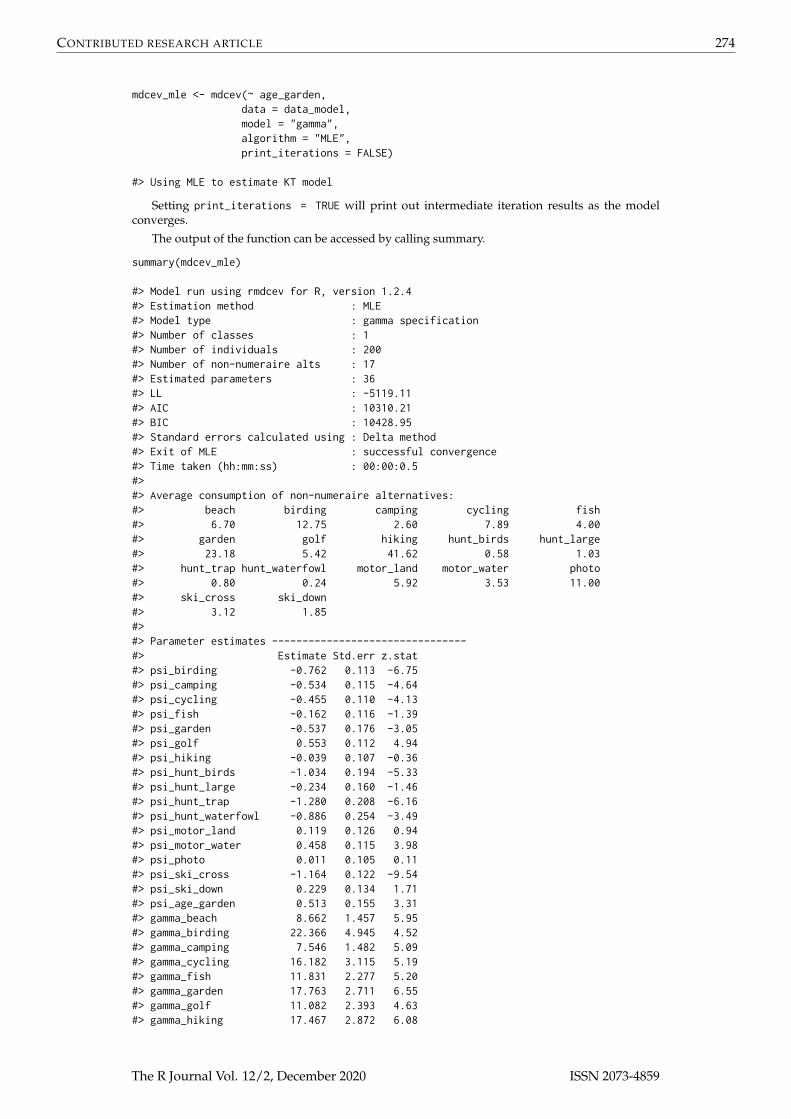
mdcev_mle <- mdcev(~ age_garden,data = data_model,model = "gamma",algorithm = "MLE",print_iterations = FALSE)

#> Using MLE to estimate KT model

Setting print_iterations = TRUE will print out intermediate iteration results as the modelconverges.

The output of the function can be accessed by calling summary.

summary(mdcev_mle)

#> Model run using rmdcev for R, version 1.2.4#> Estimation method : MLE#> Model type : gamma specification#> Number of classes : 1#> Number of individuals : 200#> Number of non-numeraire alts : 17#> Estimated parameters : 36#> LL : -5119.11#> AIC : 10310.21#> BIC : 10428.95#> Standard errors calculated using : Delta method#> Exit of MLE : successful convergence#> Time taken (hh:mm:ss) : 00:00:0.5#>#> Average consumption of non-numeraire alternatives:#> beach birding camping cycling fish#> 6.70 12.75 2.60 7.89 4.00#> garden golf hiking hunt_birds hunt_large#> 23.18 5.42 41.62 0.58 1.03#> hunt_trap hunt_waterfowl motor_land motor_water photo#> 0.80 0.24 5.92 3.53 11.00#> ski_cross ski_down#> 3.12 1.85#>#> Parameter estimates --------------------------------#> Estimate Std.err z.stat#> psi_birding -0.762 0.113 -6.75#> psi_camping -0.534 0.115 -4.64#> psi_cycling -0.455 0.110 -4.13#> psi_fish -0.162 0.116 -1.39#> psi_garden -0.537 0.176 -3.05#> psi_golf 0.553 0.112 4.94#> psi_hiking -0.039 0.107 -0.36#> psi_hunt_birds -1.034 0.194 -5.33#> psi_hunt_large -0.234 0.160 -1.46#> psi_hunt_trap -1.280 0.208 -6.16#> psi_hunt_waterfowl -0.886 0.254 -3.49#> psi_motor_land 0.119 0.126 0.94#> psi_motor_water 0.458 0.115 3.98#> psi_photo 0.011 0.105 0.11#> psi_ski_cross -1.164 0.122 -9.54#> psi_ski_down 0.229 0.134 1.71#> psi_age_garden 0.513 0.155 3.31#> gamma_beach 8.662 1.457 5.95#> gamma_birding 22.366 4.945 4.52#> gamma_camping 7.546 1.482 5.09#> gamma_cycling 16.182 3.115 5.19#> gamma_fish 11.831 2.277 5.20#> gamma_garden 17.763 2.711 6.55#> gamma_golf 11.082 2.393 4.63#> gamma_hiking 17.467 2.872 6.08



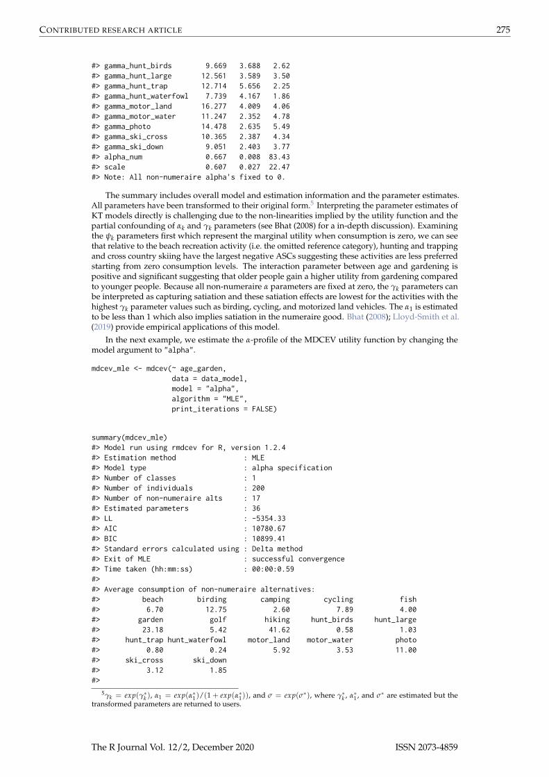
#> gamma_hunt_birds 9.669 3.688 2.62#> gamma_hunt_large 12.561 3.589 3.50#> gamma_hunt_trap 12.714 5.656 2.25#> gamma_hunt_waterfowl 7.739 4.167 1.86#> gamma_motor_land 16.277 4.009 4.06#> gamma_motor_water 11.247 2.352 4.78#> gamma_photo 14.478 2.635 5.49#> gamma_ski_cross 10.365 2.387 4.34#> gamma_ski_down 9.051 2.403 3.77#> alpha_num 0.667 0.008 83.43#> scale 0.607 0.027 22.47#> Note: All non-numeraire alpha's fixed to 0.

The summary includes overall model and estimation information and the parameter estimates.All parameters have been transformed to their original form.5 Interpreting the parameter estimates ofKT models directly is challenging due to the non-linearities implied by the utility function and thepartial confounding of αk and γk parameters (see Bhat (2008) for a in-depth discussion). Examiningthe ψk parameters first which represent the marginal utility when consumption is zero, we can seethat relative to the beach recreation activity (i.e. the omitted reference category), hunting and trappingand cross country skiing have the largest negative ASCs suggesting these activities are less preferredstarting from zero consumption levels. The interaction parameter between age and gardening ispositive and significant suggesting that older people gain a higher utility from gardening comparedto younger people. Because all non-numeraire α parameters are fixed at zero, the γk parameters canbe interpreted as capturing satiation and these satiation effects are lowest for the activities with thehighest γk parameter values such as birding, cycling, and motorized land vehicles. The α1 is estimatedto be less than 1 which also implies satiation in the numeraire good. Bhat (2008); Lloyd-Smith et al.(2019) provide empirical applications of this model.

In the next example, we estimate the α-profile of the MDCEV utility function by changing themodel argument to "alpha".

mdcev_mle <- mdcev(~ age_garden,data = data_model,model = "alpha",algorithm = "MLE",print_iterations = FALSE)

summary(mdcev_mle)#> Model run using rmdcev for R, version 1.2.4#> Estimation method : MLE#> Model type : alpha specification#> Number of classes : 1#> Number of individuals : 200#> Number of non-numeraire alts : 17#> Estimated parameters : 36#> LL : -5354.33#> AIC : 10780.67#> BIC : 10899.41#> Standard errors calculated using : Delta method#> Exit of MLE : successful convergence#> Time taken (hh:mm:ss) : 00:00:0.59#>#> Average consumption of non-numeraire alternatives:#> beach birding camping cycling fish#> 6.70 12.75 2.60 7.89 4.00#> garden golf hiking hunt_birds hunt_large#> 23.18 5.42 41.62 0.58 1.03#> hunt_trap hunt_waterfowl motor_land motor_water photo#> 0.80 0.24 5.92 3.53 11.00#> ski_cross ski_down#> 3.12 1.85#>

5γk = exp(γ∗k ), α1 = exp(α∗1)/(1 + exp(α∗1)), and σ = exp(σ∗), where γ∗k , α∗1 , and σ∗ are estimated but thetransformed parameters are returned to users.



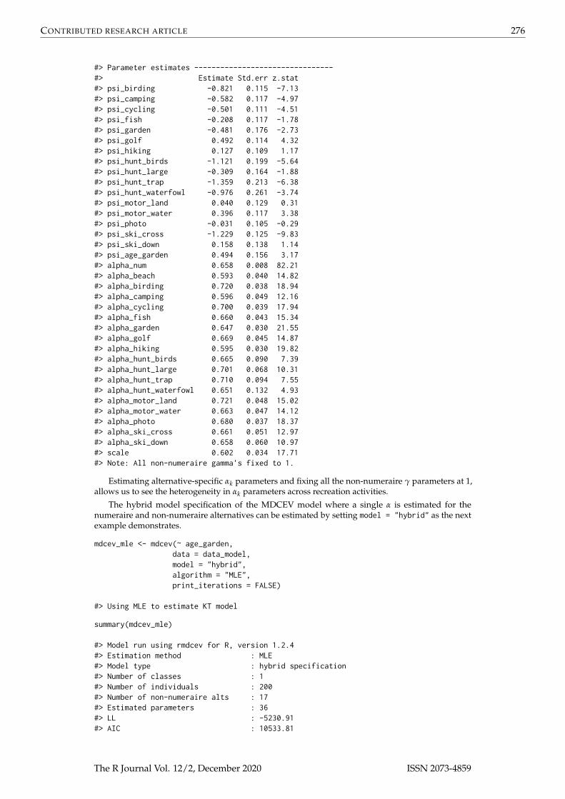
#> Parameter estimates --------------------------------#> Estimate Std.err z.stat#> psi_birding -0.821 0.115 -7.13#> psi_camping -0.582 0.117 -4.97#> psi_cycling -0.501 0.111 -4.51#> psi_fish -0.208 0.117 -1.78#> psi_garden -0.481 0.176 -2.73#> psi_golf 0.492 0.114 4.32#> psi_hiking 0.127 0.109 1.17#> psi_hunt_birds -1.121 0.199 -5.64#> psi_hunt_large -0.309 0.164 -1.88#> psi_hunt_trap -1.359 0.213 -6.38#> psi_hunt_waterfowl -0.976 0.261 -3.74#> psi_motor_land 0.040 0.129 0.31#> psi_motor_water 0.396 0.117 3.38#> psi_photo -0.031 0.105 -0.29#> psi_ski_cross -1.229 0.125 -9.83#> psi_ski_down 0.158 0.138 1.14#> psi_age_garden 0.494 0.156 3.17#> alpha_num 0.658 0.008 82.21#> alpha_beach 0.593 0.040 14.82#> alpha_birding 0.720 0.038 18.94#> alpha_camping 0.596 0.049 12.16#> alpha_cycling 0.700 0.039 17.94#> alpha_fish 0.660 0.043 15.34#> alpha_garden 0.647 0.030 21.55#> alpha_golf 0.669 0.045 14.87#> alpha_hiking 0.595 0.030 19.82#> alpha_hunt_birds 0.665 0.090 7.39#> alpha_hunt_large 0.701 0.068 10.31#> alpha_hunt_trap 0.710 0.094 7.55#> alpha_hunt_waterfowl 0.651 0.132 4.93#> alpha_motor_land 0.721 0.048 15.02#> alpha_motor_water 0.663 0.047 14.12#> alpha_photo 0.680 0.037 18.37#> alpha_ski_cross 0.661 0.051 12.97#> alpha_ski_down 0.658 0.060 10.97#> scale 0.602 0.034 17.71#> Note: All non-numeraire gamma's fixed to 1.

Estimating alternative-specific αk parameters and fixing all the non-numeraire γ parameters at 1,allows us to see the heterogeneity in αk parameters across recreation activities.

The hybrid model specification of the MDCEV model where a single α is estimated for thenumeraire and non-numeraire alternatives can be estimated by setting model = "hybrid" as the nextexample demonstrates.

mdcev_mle <- mdcev(~ age_garden,data = data_model,model = "hybrid",algorithm = "MLE",print_iterations = FALSE)


summary(mdcev_mle)

#> Model run using rmdcev for R, version 1.2.4#> Estimation method : MLE#> Model type : hybrid specification#> Number of classes : 1#> Number of individuals : 200#> Number of non-numeraire alts : 17#> Estimated parameters : 36#> LL : -5230.91#> AIC : 10533.81



#> BIC : 10652.55#> Standard errors calculated using : Delta method#> Exit of MLE : successful convergence#> Time taken (hh:mm:ss) : 00:00:0.6#>#> Average consumption of non-numeraire alternatives:#> beach birding camping cycling fish#> 6.70 12.75 2.60 7.89 4.00#> garden golf hiking hunt_birds hunt_large#> 23.18 5.42 41.62 0.58 1.03#> hunt_trap hunt_waterfowl motor_land motor_water photo#> 0.80 0.24 5.92 3.53 11.00#> ski_cross ski_down#> 3.12 1.85#>#> Parameter estimates --------------------------------#> Estimate Std.err z.stat#> psi_birding -0.783 0.081 -9.67#> psi_camping -0.570 0.082 -6.95#> psi_cycling -0.488 0.078 -6.25#> psi_fish -0.206 0.083 -2.48#> psi_garden -0.580 0.128 -4.53#> psi_golf 0.565 0.080 7.06#> psi_hiking -0.285 0.076 -3.75#> psi_hunt_birds -0.832 0.137 -6.08#> psi_hunt_large -0.095 0.113 -0.84#> psi_hunt_trap -1.029 0.146 -7.05#> psi_hunt_waterfowl -0.524 0.178 -2.94#> psi_motor_land 0.172 0.090 1.91#> psi_motor_water 0.449 0.082 5.48#> psi_photo -0.103 0.074 -1.39#> psi_ski_cross -1.112 0.087 -12.78#> psi_ski_down 0.345 0.095 3.63#> psi_age_garden 0.312 0.112 2.79#> gamma_beach 2.198 0.446 4.93#> gamma_birding 5.722 1.484 3.86#> gamma_camping 2.669 0.649 4.11#> gamma_cycling 5.745 1.307 4.40#> gamma_fish 4.162 1.007 4.13#> gamma_garden 4.776 0.910 5.25#> gamma_golf 3.446 0.873 3.95#> gamma_hiking 3.315 0.719 4.61#> gamma_hunt_birds 3.719 1.704 2.18#> gamma_hunt_large 5.533 1.922 2.88#> gamma_hunt_trap 4.605 2.446 1.88#> gamma_hunt_waterfowl 3.227 2.029 1.59#> gamma_motor_land 5.691 1.642 3.47#> gamma_motor_water 3.941 1.011 3.90#> gamma_photo 4.723 1.012 4.67#> gamma_ski_cross 3.593 0.994 3.61#> gamma_ski_down 3.265 1.027 3.18#> alpha 0.648 0.005 129.53#> scale 0.431 0.014 30.78#> Note: Alpha parameter is equal for all alternatives.

The same number of parameters are estimated in all three models and the log-likelihood is highestfor the γ-profile specification. The ease of estimating different MDCEV model specifications canbe used to compare models quickly and help the analyst pick their preferred specification for eachempirical application.

We can also estimate the KT-EE specification by changing the formula call and the model call to"kt_ee".

kt_mle <- mdcev(~ age_garden | 0 | 0,data = data_model,model = "kt_ee",



algorithm = "MLE",print_iterations = FALSE)

summary(kt_mle)

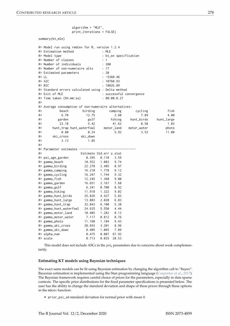
#> Model run using rmdcev for R, version 1.2.4#> Estimation method : MLE#> Model type : kt_ee specification#> Number of classes : 1#> Number of individuals : 200#> Number of non-numeraire alts : 17#> Estimated parameters : 20#> LL : -5360.46#> AIC : 10760.93#> BIC : 10826.89#> Standard errors calculated using : Delta method#> Exit of MLE : successful convergence#> Time taken (hh:mm:ss) : 00:00:0.27#>#> Average consumption of non-numeraire alternatives:#> beach birding camping cycling fish#> 6.70 12.75 2.60 7.89 4.00#> garden golf hiking hunt_birds hunt_large#> 23.18 5.42 41.62 0.58 1.03#> hunt_trap hunt_waterfowl motor_land motor_water photo#> 0.80 0.24 5.92 3.53 11.00#> ski_cross ski_down#> 3.12 1.85#>#> Parameter estimates --------------------------------#> Estimate Std.err z.stat#> psi_age_garden 0.395 0.110 3.59#> gamma_beach 10.552 1.083 9.74#> gamma_birding 22.278 2.485 8.97#> gamma_camping 16.210 1.778 9.12#> gamma_cycling 16.247 1.744 9.32#> gamma_fish 12.245 1.360 9.00#> gamma_garden 16.651 2.167 7.68#> gamma_golf 6.241 0.700 8.92#> gamma_hiking 11.918 1.322 9.02#> gamma_hunt_birds 25.826 4.427 5.83#> gamma_hunt_large 13.803 2.020 6.83#> gamma_hunt_trap 32.843 6.100 5.38#> gamma_hunt_waterfowl 24.635 5.550 4.44#> gamma_motor_land 10.405 1.282 8.12#> gamma_motor_water 7.117 0.812 8.76#> gamma_photo 11.160 1.184 9.43#> gamma_ski_cross 28.693 3.201 8.96#> gamma_ski_down 8.405 1.065 7.89#> alpha_num 0.475 0.007 67.92#> scale 0.713 0.025 28.53

This model does not include ASCs in the psik parameters due to concerns about weak complemen-tarity.

Estimating KT models using Bayesian techniques

The exact same models can be fit using Bayesian estimation by changing the algorithm call to "Bayes".Bayesian estimation is implemented using the Stan programming language (Carpenter et al., 2017).The Bayesian framework requires careful choice of priors for the parameters, especially in data sparsecontexts. The specific prior distributions for the fixed parameter specifications is presented below. Theuser has the ability to change the standard deviation and shape of these priors through these optionsin the mdcev function:

• prior_psi_sd standard deviation for normal prior with mean 0.



• prior_phi_sd standard deviation for normal prior with mean 0.• prior_gamma_sd standard deviation for half-normal prior with mean 1.• prior_alpha_shape shape parameter for beta distribution.• prior_scale_sd standard deviation for half-normal prior with mean 0.

For the random parameter model specifications, the priors for the means of all random parametersfollow a normal distribution with mean 0 on the unconstrained space.

There are also a number of further options for Bayesian estimation. For example, the numberof iterations (n_iterations), number of chains (n_chains), and number of cores (n_cores) for parallelimplementation of the chains can also be chosen. The full set of options for Bayesian estimation arepresented below.

• random_parameters The form of the covariance matrix for the parameters. Options are

– ‘fixed’ for no random parameters,– ’uncorr for uncorrelated random parameters, or– ‘corr’ for correlated random parameters.

• n_iterations The number of iterations to use in Bayesian estimation. The default is for thenumber of iterations to be split evenly between warmup and posterior draws. The number ofwarmup draws can be directly controlled using the warmup argument (see rstan::sampling)

• n_chains The number of independent Markov chains in Bayesian estimation.

• n_cores The number of cores used to execute the Markov chains in parallel in Bayesian estima-tion. Can set using options(mc.cores = parallel::detectCores()).

• lkj_shape_prior Prior for Cholesky matrix for correlated random parameters.

In this example, we estimate the γ-profile of the MDCEV specification using Bayesian techniques.We set the number of iterations to 200 and use 4 independent chains across 4 cores.

mdcev_bayes <- mdcev(~ age_garden,data = data_model,model = "gamma",algorithm = "Bayes",n_iterations = 200,n_chains = 4,n_cores = 4,print_iterations = FALSE)

The output of the function can be accessed by calling summary.

summary(mdcev_bayes)

#> Model run using rmdcev for R, version 1.2.4#> Estimation method : Bayes#> Model type : gamma specification#> Number of classes : 1#> Number of individuals : 200#> Number of non-numeraire alts : 17#> Estimated parameters : 36#> LL : -5137.78#> Number of chains : 4#> Number of warmup draws per chain : 100#> Total post-warmup sample : 400#> Time taken (hh:mm:ss) : 00:00:41#>#> Average consumption of non-numeraire alternatives:#> beach birding camping cycling fish#> 6.70 12.75 2.60 7.89 4.00#> garden golf hiking hunt_birds hunt_large#> 23.18 5.42 41.62 0.58 1.03#> hunt_trap hunt_waterfowl motor_land motor_water photo#> 0.80 0.24 5.92 3.53 11.00#> ski_cross ski_down#> 3.12 1.85#>



#> Parameter estimates --------------------------------#> Estimate Std.dev z.stat n_eff Rhat#> psi_birding -0.789 0.113 -7.00 255 0.99#> psi_camping -0.574 0.123 -4.67 258 1.01#> psi_cycling -0.489 0.118 -4.16 276 1.00#> psi_fish -0.206 0.123 -1.68 157 1.01#> psi_garden -0.562 0.196 -2.86 347 1.01#> psi_golf 0.501 0.134 3.74 201 1.01#> psi_hiking 0.025 0.117 0.21 429 1.00#> psi_hunt_birds -1.159 0.200 -5.80 235 1.01#> psi_hunt_large -0.344 0.179 -1.91 189 1.02#> psi_hunt_trap -1.436 0.245 -5.87 271 1.00#> psi_hunt_waterfowl -1.098 0.291 -3.77 187 1.00#> psi_motor_land 0.060 0.136 0.44 301 1.00#> psi_motor_water 0.420 0.125 3.37 277 1.00#> psi_photo -0.010 0.125 -0.08 312 1.00#> psi_ski_cross -1.222 0.135 -9.06 207 1.01#> psi_ski_down 0.153 0.147 1.04 362 1.00#> psi_age_garden 0.563 0.175 3.22 481 1.00#> gamma_beach 8.013 1.362 5.88 261 1.01#> gamma_birding 17.715 3.298 5.37 516 1.00#> gamma_camping 7.128 1.347 5.29 459 1.00#> gamma_cycling 14.506 2.756 5.26 614 1.00#> gamma_fish 11.002 2.110 5.21 636 1.00#> gamma_garden 15.587 2.546 6.12 685 0.99#> gamma_golf 10.145 2.029 5.00 399 1.00#> gamma_hiking 15.158 2.444 6.20 687 1.00#> gamma_hunt_birds 9.479 3.372 2.81 254 1.00#> gamma_hunt_large 11.702 3.016 3.88 320 1.01#> gamma_hunt_trap 11.582 3.582 3.23 252 1.01#> gamma_hunt_waterfowl 8.269 3.551 2.33 141 1.01#> gamma_motor_land 14.258 3.252 4.39 511 1.00#> gamma_motor_water 10.392 2.260 4.60 485 1.00#> gamma_photo 13.013 2.398 5.43 595 0.99#> gamma_ski_cross 9.652 2.310 4.18 527 1.00#> gamma_ski_down 8.814 2.344 3.76 357 1.00#> alpha_num 0.668 0.008 82.15 296 1.00#> scale 0.654 0.029 22.75 187 1.01#> Note: All non-numeraire alpha's fixed to 0.#> Note from Rstan: 'For each parameter, n_eff is a crude measure of effective sample#> size, and Rhat is the potential scale reduction factor on split chains (at#> convergence, Rhat=1)'

Comparing these parameter values to the maximum likelihood estimates of the γ-profile MDCEVspecification, the values are quite similar. As the data set is rather small with only 200 individuals, thepriors play a role in reducing the estimates closer to 1 for the γk, but this role will lessen in larger dataapplications.

One benefit of using the Bayesian approach is that one can take advantage of the postestimationcommands, interactive diagnostics, and posterior analysis in rstan, bayesplot (Gabry et al., 2019), andshinystan (Muth et al., 2018). For example, the effective sample size reports the estimated numberof independent draws from the posterior distribution for each parameter (Stan Development Team,2019). The interested reader is referred to these packages for additional details.

Estimating LC-KT models

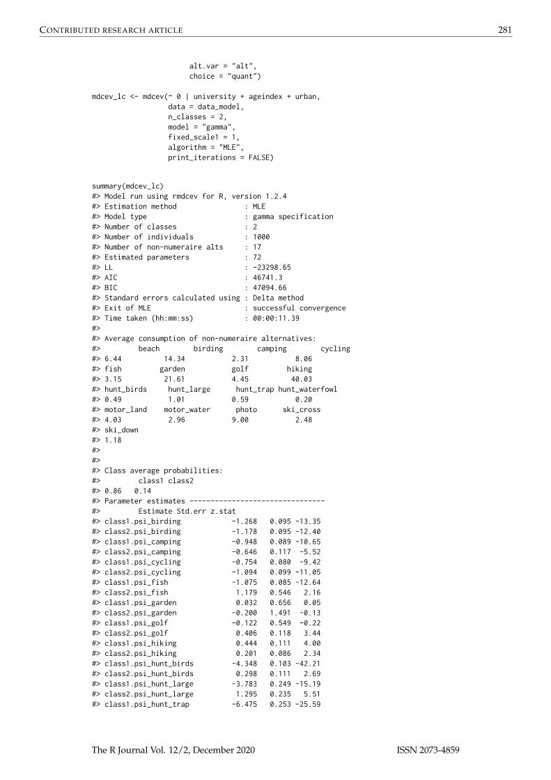
In this example, we estimate a LC-KT model using the Recreation data. We set the number of classesequal to 2 and we use data on 1000 individuals. We would like to include the university, ageindex,and urban in the membership equation and we include them in the formula interface. The constantfor the membership equation is included automatically. The LC model is automatically estimated aslong as the prespecified number of classes (n_classes) is set greater than 1. The scale parameters arefixed at 1 using fixed_scale1 = 1.

data_model <- mdcev.data(data_rec, subset = id <= 1000,id.var = "id",


https://CRAN.R-project.org/package=rstan

https://mc-stan.org/bayesplot/

https://CRAN.R-project.org/package=bayesplot

http://mc-stan.org/shinystan/

https://CRAN.R-project.org/package=shinystan


alt.var = "alt",choice = "quant")

mdcev_lc <- mdcev(~ 0 | university + ageindex + urban,data = data_model,n_classes = 2,model = "gamma",fixed_scale1 = 1,algorithm = "MLE",print_iterations = FALSE)

summary(mdcev_lc)#> Model run using rmdcev for R, version 1.2.4#> Estimation method : MLE#> Model type : gamma specification#> Number of classes : 2#> Number of individuals : 1000#> Number of non-numeraire alts : 17#> Estimated parameters : 72#> LL : -23298.65#> AIC : 46741.3#> BIC : 47094.66#> Standard errors calculated using : Delta method#> Exit of MLE : successful convergence#> Time taken (hh:mm:ss) : 00:00:11.39#>#> Average consumption of non-numeraire alternatives:#> beach birding camping cycling#> 6.44 14.34 2.31 8.06#> fish garden golf hiking#> 3.15 21.61 4.45 40.03#> hunt_birds hunt_large hunt_trap hunt_waterfowl#> 0.49 1.01 0.59 0.20#> motor_land motor_water photo ski_cross#> 4.03 2.96 9.00 2.48#> ski_down#> 1.18#>#>#> Class average probabilities:#> class1 class2#> 0.86 0.14#> Parameter estimates --------------------------------#> Estimate Std.err z.stat#> class1.psi_birding -1.268 0.095 -13.35#> class2.psi_birding -1.178 0.095 -12.40#> class1.psi_camping -0.948 0.089 -10.65#> class2.psi_camping -0.646 0.117 -5.52#> class1.psi_cycling -0.754 0.080 -9.42#> class2.psi_cycling -1.094 0.099 -11.05#> class1.psi_fish -1.075 0.085 -12.64#> class2.psi_fish 1.179 0.546 2.16#> class1.psi_garden 0.032 0.656 0.05#> class2.psi_garden -0.200 1.491 -0.13#> class1.psi_golf -0.122 0.549 -0.22#> class2.psi_golf 0.406 0.118 3.44#> class1.psi_hiking 0.444 0.111 4.00#> class2.psi_hiking 0.201 0.086 2.34#> class1.psi_hunt_birds -4.348 0.103 -42.21#> class2.psi_hunt_birds 0.298 0.111 2.69#> class1.psi_hunt_large -3.783 0.249 -15.19#> class2.psi_hunt_large 1.295 0.235 5.51#> class1.psi_hunt_trap -6.475 0.253 -25.59



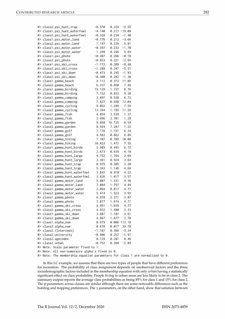
#> class2.psi_hunt_trap -0.570 0.224 -2.55#> class1.psi_hunt_waterfowl -4.140 0.217 -19.08#> class2.psi_hunt_waterfowl -0.328 0.234 -1.40#> class1.psi_motor_land -0.776 0.212 -3.66#> class2.psi_motor_land 1.147 0.229 5.01#> class1.psi_motor_water -0.397 0.233 -1.70#> class2.psi_motor_water 1.399 0.246 5.69#> class1.psi_photo -0.207 0.266 -0.78#> class2.psi_photo -0.653 0.221 -2.95#> class1.psi_ski_cross -1.772 0.209 -8.48#> class2.psi_ski_cross -1.288 0.247 -5.21#> class1.psi_ski_down -0.473 0.245 -1.93#> class2.psi_ski_down -0.388 0.282 -1.38#> class1.gamma_beach 4.112 0.372 11.05#> class2.gamma_beach 6.337 0.850 7.45#> class1.gamma_birding 15.129 1.727 8.76#> class2.gamma_birding 7.732 0.833 9.28#> class1.gamma_camping 3.497 0.520 6.73#> class2.gamma_camping 7.827 0.650 12.04#> class1.gamma_cycling 9.862 1.299 7.59#> class2.gamma_cycling 13.344 1.185 11.26#> class1.gamma_fish 4.854 3.539 1.37#> class2.gamma_fish 3.496 2.701 1.29#> class1.gamma_garden 9.858 16.725 0.59#> class2.gamma_garden 8.924 7.287 1.22#> class1.gamma_golf 7.178 1.151 6.24#> class2.gamma_golf 4.562 0.662 6.89#> class1.gamma_hiking 7.107 0.705 10.08#> class2.gamma_hiking 10.823 1.472 7.35#> class1.gamma_hunt_birds 2.989 0.445 6.72#> class2.gamma_hunt_birds 2.673 0.639 4.18#> class1.gamma_hunt_large 4.752 1.764 2.69#> class2.gamma_hunt_large 3.361 0.924 3.64#> class1.gamma_hunt_trap 0.975 0.305 3.20#> class2.gamma_hunt_trap 5.343 1.146 4.66#> class1.gamma_hunt_waterfowl 3.842 0.910 4.22#> class2.gamma_hunt_waterfowl 3.626 1.017 3.57#> class1.gamma_motor_land 5.807 1.331 4.36#> class2.gamma_motor_land 7.884 1.757 4.49#> class1.gamma_motor_water 3.894 0.817 4.77#> class2.gamma_motor_water 5.414 1.523 3.55#> class1.gamma_photo 6.970 2.271 3.07#> class2.gamma_photo 7.877 1.674 4.71#> class1.gamma_ski_cross 4.951 1.039 4.77#> class2.gamma_ski_cross 4.932 1.480 3.33#> class1.gamma_ski_down 3.887 1.107 3.51#> class2.gamma_ski_down 4.667 1.677 2.78#> class1.alpha_num 0.679 0.006 113.18#> class2.alpha_num 0.676 0.017 39.78#> class2.(Intercept) -1.187 0.366 -3.24#> class2.university -0.506 0.257 -1.97#> class2.ageindex 0.129 0.281 0.46#> class2.urban -0.752 0.260 -2.89#> Note: Scale parameter fixed to 1.#> Note: All non-numeraire alpha's fixed to 0.#> Note: The membership equation parameters for class 1 are normalized to 0.

In this LC example, we assume that there are two types of people that have different preferencesfor recreation. The probability of class assignment depends on unobserved factors and the threesociodemographic factors included in the membership equation with only urban having a statisticallysignificant effect on class probability. People living in urban areas are less likely to be in class 2. Thesummary output reports the average class probabilities as being 85% for class 1 and 15% for class 2.The ψ parameters across classes are similar although there are some noticeable differences such as thehunting and trapping preferences. The γ parameters, on the other hand, show that satiation between



classes is quite different. Sobhani et al. (2013); Kuriyama et al. (2010) provide empirical applications ofthese models.

If initial.parameter are not provided, the default is to use slightly adjusted parameter estimatesof the MDCEV model as starting values when estimating the LC-MDCEV model to assist speed andconvergence issues.6 The MDCEV model output can be accessed from mdcev_lc[["mdcev_fit"]]object for comparison.

Estimating RP-KT models

Random parameter models require defining and parameterizing the variance covariance matrix.For uncorrelated random parameters, the diagonal elements of the variance covariance matrix areestimated and the off-diagonal elements are assumed to be zero. For correlated random parameters,the variance covariance matrix is fully estimated and can be parameterized in many ways. The rmdcevpackage defines the variance covariance matrix in terms of Cholesky factors of the correlation matrixand a vector of standard deviations for numerical stability. Thus the variance covariance matrix isspecified as

∑ = diag(τ) x LLT x diag(τ), (17)

where τ is a vector of standard deviations, and L is the cholesky factors of the correlation matrix.

In this example, we estimate an uncorrelated random parameters γ-specification of the MDCEVmodel without any ψk parameters. We set the argument random_parameters = "uncorr" to indicatethat uncorrelated random parameters will be estimated. As noted earlier, all random parametersfollow a normal distribution. We change the psi_ascs = 0 to omit the ASCs in the ψk parameters.

data_model <- mdcev.data(data_rec, subset = id <= 200,id.var = "id",alt.var = "alt",choice = "quant")

mdcev_rp <- mdcev(~ 0,data = data_model,model = "gamma",algorithm = "Bayes",n_chains = 4,psi_ascs = 0,fixed_scale1 = 1,n_iterations = 200,random_parameters = "uncorr",print_iterations = FALSE)

summary(mdcev_rp)

#> Model run using rmdcev for R, version 1.2.4#> Estimation method : Bayes#> Model type : gamma specification#> Number of classes : 1#> Number of individuals : 200#> Number of non-numeraire alts : 17#> Estimated parameters : 36#> LL : -5363.25#> Random parameters : uncorrelated random parameters#> Number of chains : 4#> Number of warmup draws per chain : 100#> Total post-warmup sample : 400#> Time taken (hh:mm:ss) : 00:01:51.2#>#> Average consumption of non-numeraire alternatives:#> beach birding camping cycling fish#> 6.70 12.75 2.60 7.89 4.00#> garden golf hiking hunt_birds hunt_large#> 23.18 5.42 41.62 0.58 1.03

6In particular, the estimated ψk and γk parameters from the MDCEV model are randomly adjusted by 0.02.



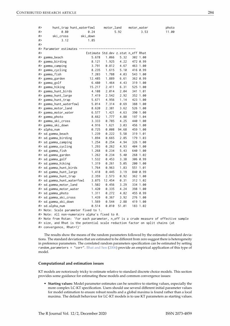
#> hunt_trap hunt_waterfowl motor_land motor_water photo#> 0.80 0.24 5.92 3.53 11.00#> ski_cross ski_down#> 3.12 1.85#>#> Parameter estimates --------------------------------#> Estimate Std.dev z.stat n_eff Rhat#> gamma_beach 5.678 1.066 5.32 302 1.00#> gamma_birding 8.121 1.925 4.22 472 0.99#> gamma_camping 3.791 0.812 4.67 463 1.00#> gamma_cycling 8.235 1.615 5.10 416 0.99#> gamma_fish 7.203 1.788 4.03 543 1.00#> gamma_garden 12.485 1.889 6.61 362 0.99#> gamma_golf 6.480 1.464 4.43 319 1.00#> gamma_hiking 15.217 2.411 6.31 525 1.00#> gamma_hunt_birds 4.108 2.014 2.04 341 1.01#> gamma_hunt_large 7.419 2.542 2.92 352 1.00#> gamma_hunt_trap 5.671 4.956 1.14 423 1.00#> gamma_hunt_waterfowl 5.014 7.314 0.69 388 1.00#> gamma_motor_land 8.620 2.381 3.62 526 1.00#> gamma_motor_water 6.577 1.421 4.63 390 1.00#> gamma_photo 8.662 1.777 4.88 197 1.04#> gamma_ski_cross 3.333 0.785 4.25 440 1.00#> gamma_ski_down 4.916 1.621 3.03 456 1.00#> alpha_num 0.725 0.008 94.68 459 1.00#> sd.gamma_beach 1.239 0.222 5.58 319 1.01#> sd.gamma_birding 1.894 0.665 2.85 179 1.03#> sd.gamma_camping 1.254 0.254 4.94 326 1.00#> sd.gamma_cycling 1.293 0.262 4.93 404 1.00#> sd.gamma_fish 1.268 0.234 5.43 640 1.00#> sd.gamma_garden 1.262 0.234 5.40 268 1.02#> sd.gamma_golf 1.532 0.453 3.38 306 0.99#> sd.gamma_hiking 1.319 0.261 5.05 200 1.00#> sd.gamma_hunt_birds 1.764 0.963 1.83 551 1.01#> sd.gamma_hunt_large 1.418 0.445 3.19 840 0.99#> sd.gamma_hunt_trap 2.359 2.573 0.92 362 1.00#> sd.gamma_hunt_waterfowl 3.875 12.454 0.31 312 1.02#> sd.gamma_motor_land 1.502 0.456 3.29 334 1.00#> sd.gamma_motor_water 1.420 0.335 4.24 398 1.00#> sd.gamma_photo 1.311 0.272 4.82 455 0.99#> sd.gamma_ski_cross 1.439 0.367 3.92 276 1.00#> sd.gamma_ski_down 1.569 0.544 2.88 419 1.00#> sd.alpha_num 0.514 0.010 51.01 183 1.02#> Note: Scale parameter fixed to 1.#> Note: All non-numeraire alpha's fixed to 0.#> Note from Rstan: 'For each parameter, n_eff is a crude measure of effective sample#> size, and Rhat is the potential scale reduction factor on split chains (at#> convergence, Rhat=1)'

The results show the means of the random parameters followed by the estimated standard devia-tions. The standard deviations that are estimated to be different from zero suggest there is heterogeneityin preference parameters. The correlated random parameters specification can be estimated by settingrandom_parameters = "corr". Bhat and Sen (2006) provide an empirical application of this type ofmodel.

Computational and estimation issues

KT models are notoriously tricky to estimate relative to standard discrete choice models. This sectionprovides some guidance for estimating these models and common convergence issues:

• Starting values: Model parameter estimates can be sensitive to starting values, especially themore complex LC-KT specification. Users should use several different initial parameter valuesfor model estimation to ensure robust results and a global maxima is found rather than a localmaxima. The default behaviour for LC-KT models is to use KT parameters as starting values.



In practice the author has found this to be quite effective at finding global maxima. However,users are encouraged to use random starting values as a robustness check.

• Identification issues: Depending on the model specification and included variables the modelmay not be properly identified. If you receive an error such as Error in chol.default(-H): the leading minor of order 9 is not positive definite or In sqrt(diag(cov_mat)): NaNs produced, this usually suggests an identification issue. Users should double check allvariables included in the model are appropriate. One solution is to start with a simpler modelfirst and then slowly add variables to help locate any problematic variables.

• Parameter estimates near boundaries: Interpret models with parameter estimates that are nearthe boundaries (e.g. α close to 1) with caution. Users are recommended to re-estimate the modelwith starting values far from this boundary.

• Bayesian estimation: For models estimated using Bayesian estimation, users should consultthe rstan User Guide for additional guidance on model estimation options and postestima-tion checks (Stan Development Team, 2019). Additional information is available by typinghelp(rstan).

Simulating KT demand and welfare scenarios

The rmdcev package includes simulation functions for calculating welfare measures and forecastingdemand under alternative policy scenarios. The overall approach used for simulation is first introducedand then code examples are given.

Overview of simulation steps

Once the model parameters are estimated, there are two steps to simulation in KT models. In thefirst step we draw simulated values for the unobserved heterogeneity term (ε) using Monte Carlotechniques. The second step uses these error draws, the previously estimated model parameters, andthe underlying data to calculate Marshallian demands for forecasting or Hicksian demands for welfareanalysis. These two steps are described below.

Step 1: simulating unobserved heterogeneity

Monte Carlo simulation techniques can be employed to draw simulated values of the unobservedheterogeneity (ε) using either unconditional or conditional draws.

1. Unconditional error draws: draw from the entire distribution of unobserved heterogeneityusing the following formula

εk = −log(−log(draw(0, 1))) ∗ σ, (18)

where draw(0, 1) is a draw between 0 and 1 and σ is the scale parameter. rmdcev allows errorsto be drawn using uniform draws or the Modified Latin Hypercube Sampling algorithm (Hess et al.,2006).

2. Conditional error draws: draw errors terms to reflect behaviour and dependent on whetheralternative is consumed or not (von Haefen, 2003; von Haefen et al., 2004):

• If xk > 0, set εk = (V1 − Vk)/σ for the MDCEV specifications where V1 and Vk depend onthe model specification as detailed above. If using the environmental economics KT modelspecification (“kt_ee”), set εk = gk(.) from Equation (12).

• If xk = 0, εk < (V1−Vk)/σ and simulate εk from the truncated type I extreme value distributionsuch that

εk = −log(−log(draw(0, 1) ∗ exp(−exp(V1 −Vk

σ)))) ∗ σ for the MDCEV specifications, or (19)

εk = −log(−log(draw(0, 1) ∗ exp(−exp(−gk(.))))) ∗ σ for the KT-EE specification. (20)

In the conditional error draw approach, we normalize ε1 = 0.

The main differences between these two error draw approaches is that in the conditional approach,errors are drawn such that the model perfectly predicts the observed consumption patterns in thebaseline state (von Haefen and Phaneuf, 2005). The conditional approach uses observed behaviour by



individuals to characterize unobserved heterogeneity and can be useful for scenario simulation as thebaseline matches observed behavior. This is especially true if poor in-sample behavioral predictions isfound using the unconditional approach (von Haefen, 2003). The unconditional approach draws allerrors based on distributional assumptions and is necessary for out-of-sample forecasting. If the modelcorrectly specifies the data generating process, the sample means of the conditional and unconditionalapproaches should converge in expectation. Another difference between the two approaches is thatthe unconditional approach uses more computation time as there is a need to calculate consumptionpatterns in the baseline state as well as simulate the entire distribution of unobserved heterogeneity.

Step 2: Calculating welfare measures and demand forecasts

With the error draws in hand, the second step is to simulate demand or welfare changes. Comparedto welfare measures in discrete choice models, welfare calculation in KT models is more challengingbecause of the two KT conditions in Equation (2). For a given policy scenario, a priori, we do not knowwhich alternatives have a positive or zero consumption level. rmdcev implements the Pinjari and Bhat(2011) efficient demand forecasting routine for simulating demand behaviour for MDCEV modelswhich relies on calculating Marshallian demands. For welfare calculations, we need to calculatethe expenditure function in Equation (3) which relies on Hicksian demands. These are calculatedusing the approach described by Lloyd-Smith (2018) and the rmdcev extends these approaches to theenvironmental economics KT model specifications. The demand and welfare simulation approachesshare a lot of commonalities and thus only the approach used for welfare calculations are fullydescribed in the appendix. The specific steps for demand simulation is explained in-depth in Pinjariand Bhat (2011) and the interested reader is encouraged to read Section 4 of the paper for the exactdetails.

Welfare analysis

In rmdcev, the functions for welfare and demand simulation have been divided into 3 steps to allowusers to parallelize operations as necessary.

We first estimate the model using mdcev and we set std_errors = "mvn" to generate multivariatenormal draws as these will be required to generate standard errors for calculations.

mdcev_mle <- mdcev(~ageindex,data = data_model,model = "hybrid",algorithm = "MLE",std_errors = "mvn",print_iterations = FALSE)


1. Define policy scenarios In the first step, we define the number of alternative policy scenariosto use in simulation and then specify changes to the ψ variables and prices of alternatives. TheCreateBlankPolicies function has been created to easily set-up the required lists for the simulation.These policies can then be manually edited according to the specific policy scenario. For prices, rmdcevis set up to accept additive changes in prices that impact all individuals the same. For the ψ and φvariable changes, the package is set up to accept any new values for these variables. Depending onthe number of individuals and number of policies, the generated policies list can be quite large. If theuser is only interested in assessing price changes, then you can use price_change_only = TRUE whichensures duplicate ψ and φ data is not created.

In this example, we are interested in two separate policies. The first policy increases the costs of allrecreation activities by $1 and the second policy increases the cost of all four hunting activities by $10.The policy set-up for these two scenarios is demonstrated below.

nalts <- mdcev_mle$stan_data[["J"]]npols <- 2

policies<- CreateBlankPolicies(npols = npols,model = mdcev_mle,price_change_only = TRUE)

policies$price_p[[1]] <- c(0, rep(1, nalts))policies$price_p[[2]][10:13] <- rep(10, 4)



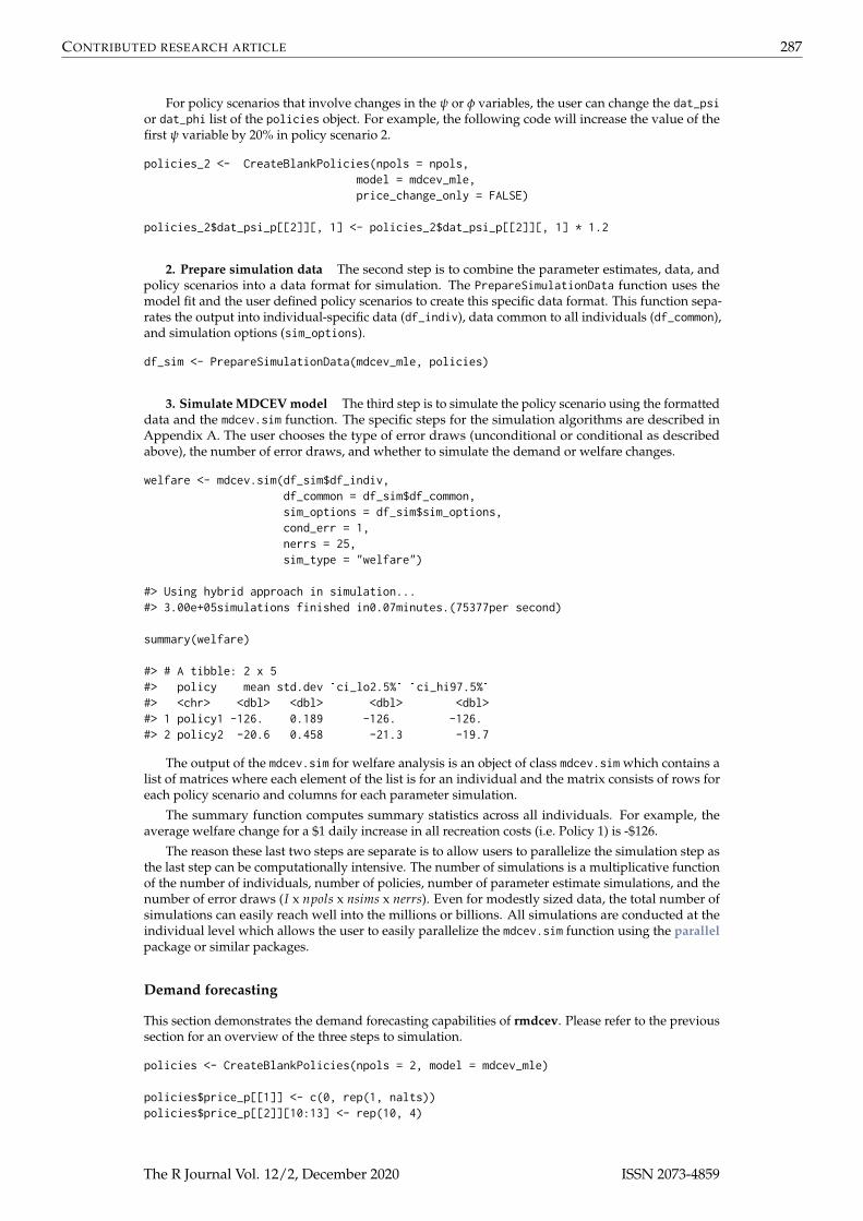
For policy scenarios that involve changes in the ψ or φ variables, the user can change the dat_psior dat_phi list of the policies object. For example, the following code will increase the value of thefirst ψ variable by 20% in policy scenario 2.

policies_2 <- CreateBlankPolicies(npols = npols,model = mdcev_mle,price_change_only = FALSE)

policies_2$dat_psi_p[[2]][, 1] <- policies_2$dat_psi_p[[2]][, 1] * 1.2

2. Prepare simulation data The second step is to combine the parameter estimates, data, andpolicy scenarios into a data format for simulation. The PrepareSimulationData function uses themodel fit and the user defined policy scenarios to create this specific data format. This function sepa-rates the output into individual-specific data (df_indiv), data common to all individuals (df_common),and simulation options (sim_options).

df_sim <- PrepareSimulationData(mdcev_mle, policies)

3. Simulate MDCEV model The third step is to simulate the policy scenario using the formatteddata and the mdcev.sim function. The specific steps for the simulation algorithms are described inAppendix A. The user chooses the type of error draws (unconditional or conditional as describedabove), the number of error draws, and whether to simulate the demand or welfare changes.

welfare <- mdcev.sim(df_sim$df_indiv,df_common = df_sim$df_common,sim_options = df_sim$sim_options,cond_err = 1,nerrs = 25,sim_type = "welfare")

#> Using hybrid approach in simulation...#> 3.00e+05simulations finished in0.07minutes.(75377per second)

summary(welfare)

#> # A tibble: 2 x 5#> policy mean std.dev `ci_lo2.5%` `ci_hi97.5%`#> <chr> <dbl> <dbl> <dbl> <dbl>#> 1 policy1 -126. 0.189 -126. -126.#> 2 policy2 -20.6 0.458 -21.3 -19.7

The output of the mdcev.sim for welfare analysis is an object of class mdcev.sim which contains alist of matrices where each element of the list is for an individual and the matrix consists of rows foreach policy scenario and columns for each parameter simulation.

The summary function computes summary statistics across all individuals. For example, theaverage welfare change for a $1 daily increase in all recreation costs (i.e. Policy 1) is -$126.

The reason these last two steps are separate is to allow users to parallelize the simulation step asthe last step can be computationally intensive. The number of simulations is a multiplicative functionof the number of individuals, number of policies, number of parameter estimate simulations, and thenumber of error draws (I x npols x nsims x nerrs). Even for modestly sized data, the total number ofsimulations can easily reach well into the millions or billions. All simulations are conducted at theindividual level which allows the user to easily parallelize the mdcev.sim function using the parallelpackage or similar packages.

Demand forecasting

This section demonstrates the demand forecasting capabilities of rmdcev. Please refer to the previoussection for an overview of the three steps to simulation.

policies <- CreateBlankPolicies(npols = 2, model = mdcev_mle)

policies$price_p[[1]] <- c(0, rep(1, nalts))policies$price_p[[2]][10:13] <- rep(10, 4)


https://CRAN.R-project.org/package=parallel


df_sim <- PrepareSimulationData(mdcev_mle, policies)

demand <- mdcev.sim(df_sim$df_indiv,df_common = df_sim$df_common,sim_options = df_sim$sim_options,cond_err = 1,nerrs = 25,sim_type = "demand")

#> Using hybrid approach in simulation...#> 5.40e+06simulations finished in0.07minutes.(1360202per second)

summary(demand)

#> # A tibble: 36 x 6#> # Groups: policy [2]#> policy alt mean std.dev `ci_lo2.5%` `ci_hi97.5%`#> <chr> <int> <dbl> <dbl> <dbl> <dbl>#> 1 policy1 0 68946. 8.62 68933. 68962.#> 2 policy1 1 6.24 0.02 6.2 6.28#> 3 policy1 2 11.2 0.05 11.1 11.2#> 4 policy1 3 2.34 0.02 2.31 2.37#> 5 policy1 4 7.24 0.04 7.18 7.3#> 6 policy1 5 3.76 0.02 3.72 3.78#> 7 policy1 6 20.7 0.06 20.7 20.8#> 8 policy1 7 5.29 0.01 5.28 5.3#> 9 policy1 8 36.1 0.15 35.8 36.4#> 10 policy1 9 0.55 0 0.53 0.55#> # ... with 26 more rows

The output of the demand simulation a mdcev.sim object with a list of I elements, one for eachindividual. Within each element there are nsim lists each containing a matrix of demands. The rowsof the matrix are for each policy scenario and the columns represent each alternative. The summaryfunction computes summary statistics.

Generating simulated data

The rmdcev package has the capability to simulate KT data. Simulated KT data can be easily createdfor model assessment and Monte Carlo analysis using the GenerateMDCEVData function. The followingexample will generate a simulated data set with 1,000 individuals, 10 non-numeraire alternatives, andparticular parameter values.

model = "gamma"nobs = 1000nalts = 10sim.data <- GenerateMDCEVData(model = model,

nobs = nobs,nalts = nalts,psi_j_parms = c(-5, 0.5, 2), # alt-specific variablespsi_i_parms = c(-1.5, 3, -2, 1, 2), # individual-specific variablesgamma_parms = stats::runif(nalts, 1, 10),alpha_parms = 0.5,scale_parms = 1)


Next, we can estimate the model using maximum likelihood techniques to recover the parameterestimates.

mdcev_mle <- mdcev(formula = ~ b1 + b2 + b3 + b4 + b5 + b6 + b7 + b8,data = sim.data$data,



model = model,psi_ascs = 0,algorithm = "MLE",print_iterations = FALSE)

Conclusions

The rmdcev package implements several Kuhn-Tucker model specifications including MDCEV withheterogeneity that can be continuous (i.e. random parameters) or discrete (i.e. latent classes). Modelscan be estimated using maximum likelihood or Bayesian techniques. This paper demonstrates the useof the package to estimate several model specifications and to derive demand forecasts and welfareimplications of policy scenarios. To my knowledge, there is no other available statistical packagethat can estimate welfare implications of policy scenarios using MDCEV models. I hope that thepublication of rmdcev will make KT modeling available to a wider audience.

Appendix A: Specific steps for simulating KT models

Welfare and demand simulation follow similar approaches and this section details the welfare simula-tion approach. There are two algorithms that differ depending on the model specification. If a single αparameter is estimated (i.e. model = “hybrid” or “hybrid0”), then we can use the hybrid approachto welfare simulation. If there are heterogeneous α parameters (i.e. model = “gamma”, “alpha”, or“kt_ee”), then we can use the general approach to welfare simulation. The hybrid approach is lesscomputationally intensive and provides an exact analytical solution but the general approach canbe used with all utility specifications. The specific steps for both algorithms are described below.Additional details are provided in Lloyd-Smith (2018).

Steps in algorithm for hybrid-profile MDCEV utility specifications

Step 0: Assume that only the numeraire alternative is chosen and let the number of chosenalternatives equal one (M=1).

Step 1: Using the data, model parameters, and either conditional or unconditional simulated errorterm draws, calculate the price-normalized baseline utility values (ψk/pk) for all alternatives. Sort theK alternatives in the descending order of their price-normalized baseline utility values. Note that thenumeraire alternative is in the first place. Go to step 2.

Step 2: Compute the value of λE using the following equation:

1λE =

αU + ∑Mm=2 γmψm

∑Mm=2 γmψm

(pmψm

) αα−1

+ ψ1

(p1ψ1

) αα−1

α−1

α

. (21)

Go to step 3.

Step 3: If 1λE >

ψM+1pM+1

, go to step 4. Else if 1λE <

ψM+1pM+1

, set M = M + 1. If M < K, go back to step 2.If M = K, go to step 4.

Step 4: Compute the optimal Hicksian consumption levels for the first I alternatives in the abovedescending order using the following equations

x1 =

(p1

λEψ1

) 1α1−1

, and (22)

xm =

[(pm

λEψm

) 1αm−1

− 1

]γm, if xm > 0. (23)

Set the remaining alternative consumption levels to zero and stop.

Steps in algorithm for general utility specifications

In this context, there is no closed-form expressions for λE and we need to conduct a numericalbisection routine. The following routine describes the approach for the MDCEV utility specifications.The approach used for the KT-EE specification is omitted due to space, but the overall strategy is thesame with the only differences being the definitions for utility functions and optimal demands. Let λE

and U be estimates of λE and U and let tolλ and tolU be the tolerance levels for estimating λE and U



that can be arbitrarily small. The algorithm works as follows:

Step 0: Assume that only the numeraire is chosen and let the number of chosen alternatives equalone (M=1).

Step 1: Using the data, model parameters, and either conditional or unconditional simulated errorterm draws, calculate the price-normalized baseline utility values (ψk/pk) for all alternatives. Sort theK alternatives in the descending order of their price-normalized baseline utility values. Note that thenumeraire is in the first place. Go to step 2.

Step 2: Let 1λE

=ψM+1pM+1

and substitute λE into the following equation to obtain an estimate of U.

U =M

∑M=2

γm

αmψm

[(pm

λEψm

) αmαm−1

− 1

]+

ψ1α1

(p1

λEψ1

) α1α1−1

. (24)

Step 3: If U < U, go to step 4. Else, if U ≥ U, set 1λE

l=

ψM+1pM+1

and 1λE

u=

ψMpM

. Go to step 5.

Step 4: Set M = M + 1. If M < K, go to step 2. Else if M = K, set 1λE

l= 0 and 1

λEu=

ψKpK

. Go to step

5.

Step 5: Let λE = (λEl + λE

u )/2 and substitute λE into the equation of step 2 to obtain an estimateof U. Go to step 6.

Step 6: If |λEl − λE

u | ≤ tolλ or |U − U| ≤ tolU , go to step 7. Else if U < U, update λEu =

(λEl + λE

u )/2 and go to step 5. Else if U > U, update λEl = (λE

l + λEu )/2 and go to step 5.

Step 7: Compute the optimal Hicksian consumption levels for the first M alternatives in the abovedescending order using Equation (22). Set the remaining alternative consumption levels to zero andstop.

Acknowledgements

Thanks to Joshua K Abbott and Allen Klaiber whose codes were helpful in putting this packagetogether.

Bibliography

C. Bhat and A. Pinjari. Multiple discrete-continuous choice models: A reflective analysis and aprospective view. In S. Hess and A. Daly, editors, Handbook of Choice Modelling, chapter 19, pages427–454. Edward Elgar Publishing, 2014. [p266]

C. R. Bhat. The multiple discrete-continuous extreme value (MDCEV) model: Role of utility functionparameters, identification considerations, and model extensions. Transportation Research Part B:Methodological, 42(3):274–303, 2008. ISSN 0191-2615. URL 10.1016/j.trb.2007.06.002. [p266, 268,270, 275]

C. R. Bhat and S. Sen. Household vehicle type holdings and usage: an application of the multiplediscrete-continuous extreme value (MDCEV) model. Transportation Research Part B: Methodological,40(1):35–53, Jan. 2006. ISSN 0191-2615. URL 10.1016/j.trb.2005.01.003. [p284]

B. Carpenter, A. Gelman, M. Hoffman, D. Lee, B. Goodrich, M. Betancourt, M. Brubaker, J. Guo, P. Li,and A. Riddell. Stan: A Probabilistic Programming Language. Journal of Statistical Software, Articles,76(1):1–32, 2017. ISSN 1548-7660. URL 10.18637/jss.v076.i01. [p267, 278]

Y. Croissant. mlogit: Multinomial Logit Models, 2019. URL https://CRAN.R-project.org/package=mlogit. R package version 1.0-1. [p266]

Federal, Provincial, and Territorial Governments of Canada. 2012 Canadian Nature Survey: Awareness,participation, and expenditures in nature-based recreation, conservation, and subsistence activities.Technical report, Canadian Councils of Resource Ministers, Ottawa, ON, 2014. [p270]

J. Gabry, D. Simpson, A. Vehtari, M. Betancourt, and A. Gelman. Visualization in bayesian workflow.J. R. Stat. Soc. A, 182:389–402, 2019. URL 10.1111/rssa.12378. [p280]

J. A. Herriges, C. L. Kling, and D. J. Phaneuf. What’s the use? welfare estimates from revealedpreference models when weak complementarity does not hold. Journal of Environmental Economics


10.1016/j.trb.2007.06.002

10.1016/j.trb.2005.01.003

10.18637/jss.v076.i01



10.1111/rssa.12378


and Management, 47(1):55–70, 2004. URL https://doi.org/10.1016/S0095-0696(03)00058-5. Pub-lisher: Elsevier. [p269]

S. Hess and D. Palma. Apollo: A flexible, powerful and customisable freeware package for choicemodel estimation and application. Journal of Choice Modelling, page 100170, June 2019. ISSN1755-5345. URL 10.1016/j.jocm.2019.100170. [p266, 267]

S. Hess, K. E. Train, and J. W. Polak. On the use of a Modified Latin Hypercube Sampling (MLHS)method in the estimation of a Mixed Logit Model for vehicle choice. Transportation Research Part B:Methodological, 40(2):147–163, Feb. 2006. ISSN 0191-2615. URL 10.1016/j.trb.2004.10.005. [p285]

A. Jasra, C. C. Holmes, and D. A. Stephens. Markov chain monte carlo methods and the labelswitching problem in bayesian mixture modeling. Statist. Sci., 20(1):50–67, 02 2005. URL https://doi.org/10.1214/088342305000000016. [p270]

K. Kuriyama, M. Hanemann, and J. Hilger. A latent segmentation approach to a Kuhn-Tucker model:An application to recreation demand. Journal of Environmental Economics and Management, 60(3):209–220, Nov. 2010. ISSN 0095-0696. URL 10.1016/j.jeem.2010.05.005. [p269, 283]

P. Lloyd-Smith. A new approach to calculating welfare measures in kuhn-tucker demand models.Journal of Choice Modelling, 26:19 – 27, 2018. ISSN 1755-5345. URL https://doi.org/10.1016/j.jocm.2017.12.002. [p286, 289]

P. Lloyd-Smith. The Economic Benefits of Recreation in Canada. Canadian Journal of Economics,forthcoming. [p271]

P. Lloyd-Smith, J. K. Abbott, W. Adamowicz, and D. Willard. Decoupling the Value of Leisure Timefrom Labor Market Returns in Travel Cost Models. Journal of the Association of Environmental andResource Economists, 6(2):215–242, Jan. 2019. ISSN 2333-5955. URL 10.1086/701760. [p275]

C. Muth, Z. O. Jonah, and Gabry. User-friendly bayesian regression modeling: A tutorial with rstanarmand shinystan. The Quantitative Methods for Psychology, 14(2):99–119, 2018. URL 10.20982/tqmp.14.2.p099. [p280]

K. Mäler. Environmental Economics: A Theoretical Inquiry. Johns Hopkins University Press for Resourcesfor the Future, 1974. [p268]

A. R. Pinjari and C. R. Bhat. Computationally efficient forecasting procedures for Kuhn-Tucker con-sumer demand model systems: Application to residential energy consumption analysis. Technicalreport, Department of Civil and Environmental Engineering, University of South Florida, 2011.[p286]

M. Sarrias and R. Daziano. Multinomial Logit Models with Continuous and Discrete IndividualHeterogeneity in R: The gmnl Package. Journal of Statistical Software, 79(1):1–46, July 2017. ISSN1548-7660. URL http://dx.doi.org/10.18637/jss.v079.i02. [p266]

A. Sobhani, N. Eluru, and A. Faghih-Imani. A latent segmentation based multiple discrete continuousextreme value model. Transportation Research Part B: Methodological, 58:154–169, Dec. 2013. ISSN0191-2615. URL 10.1016/j.trb.2013.07.009. [p269, 283]

Stan Development Team. RStan: the R interface to Stan. R package version 2.19, 2019. URL https://mc-stan.org/rstan. [p280, 285]

K. Train. Discrete Choice Methods with Simulation. Cambridge University Press, 2009. [p270]

R. H. von Haefen. Incorporating observed choice into the construction of welfare measures fromrandom utility models. Journal of Environmental Economics and Management, 45(2):145–165, Mar. 2003.ISSN 0095-0696. URL 10.1016/S0095-0696(02)00047-5. [p285, 286]

R. H. von Haefen and D. J. Phaneuf. Kuhn-Tucker Demand System Approaches to Non-MarketValuation. In R. Scarpa and A. Alberini, editors, Applications of Simulation Methods in Environmentaland Resource Economics, pages 135–157. Springer Netherlands, Dordrecht, 2005. ISBN 978-1-4020-3684-2. [p266, 267, 269, 270, 285]

R. H. von Haefen, D. J. Phaneuf, and G. R. Parsons. Estimation and Welfare Analysis with LargeDemand Systems. Journal of Business & Economic Statistics, 22(2):194–205, 2004. ISSN 0735-0015.[p266, 285]


https://doi.org/10.1016/S0095-0696(03)00058-5

10.1016/j.jocm.2019.100170

10.1016/j.trb.2004.10.005

https://doi.org/10.1214/088342305000000016

https://doi.org/10.1214/088342305000000016

10.1016/j.jeem.2010.05.005

https://doi.org/10.1016/j.jocm.2017.12.002

https://doi.org/10.1016/j.jocm.2017.12.002

10.1086/701760

10.20982/tqmp.14.2.p099

10.20982/tqmp.14.2.p099

http://dx.doi.org/10.18637/jss.v079.i02

10.1016/j.trb.2013.07.009

https://mc-stan.org/rstan

https://mc-stan.org/rstan

10.1016/S0095-0696(02)00047-5


A. Zeileis and Y. Croissant. Extended Model Formulas in R: Multiple Parts and Multiple Responses.Journal of Statistical Software, 34(1):1–13, Apr. 2010. ISSN 1548-7660. URL 10.18637/jss.v034.i01.[p273]

Patrick Lloyd-SmithUniversity of SaskatchewanDepartment of Agricultural and Resource EconomicsGlobal Institute for Water SecurityRoom 3D34, Agriculture Building 51 Campus DriveSaskatoon, SK S7N 5A8 Canadahttps://plloydsmith.github.io/[email protected]


10.18637/jss.v034.i01

https://plloydsmith.github.io/

mailto:[email protected]

kuhn-tucker and multiple discrete-continuous extreme …

Documents