kumonosu - university of colorado boulder

KumoNoSuVersion 1.0; March 24, 2008

USER’S MANUAL

Eric HansenDaniel RyplVictor SaoumaDepartment of Civil Engineering,University of Colorado, BoulderBoulder, CO 80309-0428

Under Contract from:Tokyo Electric Power Service Company3-3-3 Higashiueno, Taito-ku, Tokyo 110-0015

2

DISCLAIMER OF WARRANTIES AND LIMITATION OF LIABILITIES

THIS REPORT WAS PREPARED BY THE ORGANIZATION(S) NAMED BELOW AS AN ACCOUNT OF WORK SPONSORED OR COSPONSORED BY The TOKYO ELEC-TRIC POWER SERVICE COMPANY (TEPSCO). TEPSCO ANY COSPONSOR, THE ORGANIZATION(S) NAMED BELOW, NOR ANY PERSON ACTING ON BEHALF OF ANYOF THEM:

(A) MAKES ANY WARRANTY OR REPRESENTATION WHATSOEVER, EXPRESS OR IMPLIED, (I) WITH RESPECT TO THE USE OF ANY INFORMATION, APPARATUS,METHOD, PROCESS OR SIMILAR ITEM DISCLOSED IN THIS REPORT, INCLUDING MERCHANTABILITY AND FITNESS FOR A PARTICULAR PURPOSE, OR (II) THATSUCH USE DOES NOT INFRINGE ON OR INTERFERE WITH PRIVATELY OWNED RIGHTS, INCLUDING ANY PARTY’S INTELLECTUAL PROPERTY, OR (III) THAT THISREPORT IS SUITABLE TO ANY PARTICULAR USER’S CIRCUMSTANCES; OR

(B) ASSUMES RESPONSIBILITY FOR ANY DAMAGES OR OTHER LIABILITIES WHATSOEVER (INCLUDING ANY CONSEQUENTIAL DAMAGES, EVEN IF TEPSCOOR THEIR REPRESENTATIVES HAVE BEEN ADVISED OF THE POSSIBILITY OF SUCH DAMAGES) RESULTING FROM YOUR SELECTION OR USE OF THIS REPORT ORANY INFORMATION, APPARATUS, METHOD, PROCESS OR SIMILAR ITEM DISCLOSED IN THIS REPORT.

ORGANIZATION(S) THAT PREPARED THIS REPORT:

UNIVERSITY OF COLORADO AT BOULDER

KumoNoSu User’s Manual

3

ABSTRACT

KumoNoSu is a graphical front end to T3D (a finite element mesh generator), and T3D2Merlin (anstructural analysis finite element analysis data preparation program).

KumoNoSu has been written explicitly for the Merlin finite element code, and as such has numerousbuilt-in facilities to handle both cracks and/or dams. Nevertheless, the program is general enough toaccommodate most other finite element codes.

KumoNoSu enables the user to interactively define the boundary of the structure to be meshed.Following each new boundary entity definition, the graphical display is updated. Once the boundary hasbeen completely defined, then T3D is internally invoked, and a finite element mesh is generated. In thesecond module of KumoNoSu the user specifies the specific attributes of the finite element mesh (suchas material properties, boundary conditions, incremental loads) with reference to the entity defining theboundary. This in turn will internally generate a complete input data file for the Merlin finite elementcode.


4

ACKNOWLEDGMENTS

KumoNoSu is a graphical front end to the mesh generator T3D and T3D2Merlin converter developedby Dr. Daniel Rypl.

KumoNoSu was originally developed by Dr. Eric Hansen, and subsequently modified/maintained byDr. Gary Haussmann as a front end to the computer code MERLIN, through a contract from the TokyoElectric Power Service Company (TEPSCO) with the Department of Civil Engineering of the Universityof Colorado in Boulder (Victor Saouma, P.I.).

The authors would like to acknowledge the numerous feedbacks, buggs reports and other constructivecomments of: Guido Camata, Sonia Fortuna, C. Chang, Wiwat Puatsananon, and in particular ofTakashi Shimpo and Yoshinori Yagome. It was through their numerous comments that KumoNoSu hasmatured into a solid, reliable, powerful and original program.


Contents

1 Introduction 121.1 Concepts of Boundary Representation . . . . . . . . . . . . . . . . . . . . . . . . . . . . . 12

1.1.1 Hierarchy . . . . . . . . . . . . . . . . . . . . . . . . . . . . . . . . . . . . . . . . . 131.1.2 Mesh Size/Density . . . . . . . . . . . . . . . . . . . . . . . . . . . . . . . . . . . . 14

1.2 Kumo Layout . . . . . . . . . . . . . . . . . . . . . . . . . . . . . . . . . . . . . . . . . . . 14

2 File 16

3 Define Boundary 183.1 Vertex . . . . . . . . . . . . . . . . . . . . . . . . . . . . . . . . . . . . . . . . . . . . . . . 193.2 Curve . . . . . . . . . . . . . . . . . . . . . . . . . . . . . . . . . . . . . . . . . . . . . . . 20

3.2.1 Higher Order Curves . . . . . . . . . . . . . . . . . . . . . . . . . . . . . . . . . . . 233.3 Patch . . . . . . . . . . . . . . . . . . . . . . . . . . . . . . . . . . . . . . . . . . . . . . . 243.4 Surface . . . . . . . . . . . . . . . . . . . . . . . . . . . . . . . . . . . . . . . . . . . . . . . 273.5 Region . . . . . . . . . . . . . . . . . . . . . . . . . . . . . . . . . . . . . . . . . . . . . . . 283.6 Entity Groups . . . . . . . . . . . . . . . . . . . . . . . . . . . . . . . . . . . . . . . . . . . 313.7 Mouse Vertex Creation . . . . . . . . . . . . . . . . . . . . . . . . . . . . . . . . . . . . . . 313.8 Mouse Curve Creation . . . . . . . . . . . . . . . . . . . . . . . . . . . . . . . . . . . . . . 313.9 Curve Selection . . . . . . . . . . . . . . . . . . . . . . . . . . . . . . . . . . . . . . . . . . 323.10 Patch/Surface Selection . . . . . . . . . . . . . . . . . . . . . . . . . . . . . . . . . . . . . 323.11 Master/Slave . . . . . . . . . . . . . . . . . . . . . . . . . . . . . . . . . . . . . . . . . . . 323.12 Embedded Reinforcement . . . . . . . . . . . . . . . . . . . . . . . . . . . . . . . . . . . . 333.13 Cracks . . . . . . . . . . . . . . . . . . . . . . . . . . . . . . . . . . . . . . . . . . . . . . . 35

3.13.1 Crack Segments . . . . . . . . . . . . . . . . . . . . . . . . . . . . . . . . . . . . . . 353.13.2 Discrete Cracks . . . . . . . . . . . . . . . . . . . . . . . . . . . . . . . . . . . . . . 373.13.3 Examples . . . . . . . . . . . . . . . . . . . . . . . . . . . . . . . . . . . . . . . . . 37

3.14 Crack Bridging a Truss Element . . . . . . . . . . . . . . . . . . . . . . . . . . . . . . . . 393.15 Crack Library . . . . . . . . . . . . . . . . . . . . . . . . . . . . . . . . . . . . . . . . . . . 393.16 Elastic Boundary . . . . . . . . . . . . . . . . . . . . . . . . . . . . . . . . . . . . . . . . . 403.17 Viscous Boundary . . . . . . . . . . . . . . . . . . . . . . . . . . . . . . . . . . . . . . . . 40

3.17.1 Discrete Dashpots/Nodal . . . . . . . . . . . . . . . . . . . . . . . . . . . . . . . . 403.17.2 Continuous Dashpots/Elements . . . . . . . . . . . . . . . . . . . . . . . . . . . . . 40

3.18 Lumped Masses . . . . . . . . . . . . . . . . . . . . . . . . . . . . . . . . . . . . . . . . . . 413.18.1 Westergaard-Zangaar . . . . . . . . . . . . . . . . . . . . . . . . . . . . . . . . . . 413.18.2 User-Defined . . . . . . . . . . . . . . . . . . . . . . . . . . . . . . . . . . . . . . . 42

3.19 Extrude . . . . . . . . . . . . . . . . . . . . . . . . . . . . . . . . . . . . . . . . . . . . . . 43

4 View 444.1 View Settings . . . . . . . . . . . . . . . . . . . . . . . . . . . . . . . . . . . . . . . . . . . 44

4.1.1 Viewer Config . . . . . . . . . . . . . . . . . . . . . . . . . . . . . . . . . . . . . . . 444.1.2 Selective Display . . . . . . . . . . . . . . . . . . . . . . . . . . . . . . . . . . . . . 444.1.3 Domain Display . . . . . . . . . . . . . . . . . . . . . . . . . . . . . . . . . . . . . 454.1.4 Load Display . . . . . . . . . . . . . . . . . . . . . . . . . . . . . . . . . . . . . . . 45

CONTENTS 6

4.1.5 Creation Control . . . . . . . . . . . . . . . . . . . . . . . . . . . . . . . . . . . . . 454.2 Kumonosu Settings . . . . . . . . . . . . . . . . . . . . . . . . . . . . . . . . . . . . . . . . 464.3 Settings . . . . . . . . . . . . . . . . . . . . . . . . . . . . . . . . . . . . . . . . . . . . . . 464.4 Lighting . . . . . . . . . . . . . . . . . . . . . . . . . . . . . . . . . . . . . . . . . . . . . . 464.5 Reset Camera . . . . . . . . . . . . . . . . . . . . . . . . . . . . . . . . . . . . . . . . . . . 46

5 Generate Mesh 48

6 T3D2MERLIN 496.1 Title . . . . . . . . . . . . . . . . . . . . . . . . . . . . . . . . . . . . . . . . . . . . . . . . 506.2 Keywords . . . . . . . . . . . . . . . . . . . . . . . . . . . . . . . . . . . . . . . . . . . . . 50

6.2.1 General options . . . . . . . . . . . . . . . . . . . . . . . . . . . . . . . . . . . . . . 506.2.1.1 Monitor Max/Min Stress . . . . . . . . . . . . . . . . . . . . . . . . . . . 506.2.1.2 AutoCrack . . . . . . . . . . . . . . . . . . . . . . . . . . . . . . . . . . . 506.2.1.3 MultLDCurves . . . . . . . . . . . . . . . . . . . . . . . . . . . . . . . . . 516.2.1.4 TimeAccelCurve . . . . . . . . . . . . . . . . . . . . . . . . . . . . . . . . 526.2.1.5 TimeDispCurve . . . . . . . . . . . . . . . . . . . . . . . . . . . . . . . . 536.2.1.6 Time Stress Curve . . . . . . . . . . . . . . . . . . . . . . . . . . . . . . 536.2.1.7 Time Strain Curve . . . . . . . . . . . . . . . . . . . . . . . . . . . . . . 546.2.1.8 UserCurves . . . . . . . . . . . . . . . . . . . . . . . . . . . . . . . . . . 546.2.1.9 BandwidthMin . . . . . . . . . . . . . . . . . . . . . . . . . . . . . . . . . 546.2.1.10 RealTimeView . . . . . . . . . . . . . . . . . . . . . . . . . . . . . . . . . 556.2.1.11 Restart on Increment . . . . . . . . . . . . . . . . . . . . . . . . . . . . 556.2.1.12 Do Not Write Mesh . . . . . . . . . . . . . . . . . . . . . . . . . . . . . . 556.2.1.13 InitAnalflag . . . . . . . . . . . . . . . . . . . . . . . . . . . . . . . . . 556.2.1.14 Split Output . . . . . . . . . . . . . . . . . . . . . . . . . . . . . . . . . . 556.2.1.15 Split .pst . . . . . . . . . . . . . . . . . . . . . . . . . . . . . . . . . . . . 556.2.1.16 Initial Temperature . . . . . . . . . . . . . . . . . . . . . . . . . . . . . . 55

6.2.2 Analysis Type Options . . . . . . . . . . . . . . . . . . . . . . . . . . . . . . . . . . 556.2.2.1 Implicit Transient . . . . . . . . . . . . . . . . . . . . . . . . . . . . . 556.2.2.2 Explicit Transient . . . . . . . . . . . . . . . . . . . . . . . . . . . . . 56

6.2.3 Strain Smoothing Options . . . . . . . . . . . . . . . . . . . . . . . . . . . . . . . . 586.2.4 Fracture Mechanics Options . . . . . . . . . . . . . . . . . . . . . . . . . . . . . . . 586.2.5 Print Options . . . . . . . . . . . . . . . . . . . . . . . . . . . . . . . . . . . . . . . 58

6.3 Material and Element Groups . . . . . . . . . . . . . . . . . . . . . . . . . . . . . . . . . . 596.4 AAR . . . . . . . . . . . . . . . . . . . . . . . . . . . . . . . . . . . . . . . . . . . . . . . . 606.5 Discrete/Continuum Groups . . . . . . . . . . . . . . . . . . . . . . . . . . . . . . . . . . . 606.6 Eigenmode . . . . . . . . . . . . . . . . . . . . . . . . . . . . . . . . . . . . . . . . . . . . 606.7 Loads . . . . . . . . . . . . . . . . . . . . . . . . . . . . . . . . . . . . . . . . . . . . . . . 61

6.7.1 Incremental Load Definition . . . . . . . . . . . . . . . . . . . . . . . . . . . . . . . 626.7.1.1 Displacement BC’s . . . . . . . . . . . . . . . . . . . . . . . . . . . . . . . 626.7.1.2 Body Forces . . . . . . . . . . . . . . . . . . . . . . . . . . . . . . . . . . 626.7.1.3 Point Loads . . . . . . . . . . . . . . . . . . . . . . . . . . . . . . . . . . 636.7.1.4 Tractions . . . . . . . . . . . . . . . . . . . . . . . . . . . . . . . . . . . . 646.7.1.5 Centrifugal . . . . . . . . . . . . . . . . . . . . . . . . . . . . . . . . . . . 646.7.1.6 Nodal Temperature . . . . . . . . . . . . . . . . . . . . . . . . . . . . . . 66

6.7.1.6.1 GUI Entry . . . . . . . . . . . . . . . . . . . . . . . . . . . . . . 666.7.1.6.2 External File . . . . . . . . . . . . . . . . . . . . . . . . . . . . . 67

6.7.1.7 Point (xyz) Temperatures . . . . . . . . . . . . . . . . . . . . . . . . . . . 676.7.1.7.1 GUI Specification . . . . . . . . . . . . . . . . . . . . . . . . . . 676.7.1.7.2 External File Input . . . . . . . . . . . . . . . . . . . . . . . . . 67

6.7.2 Total Load Definition . . . . . . . . . . . . . . . . . . . . . . . . . . . . . . . . . . 686.7.2.1 Hydrostatic . . . . . . . . . . . . . . . . . . . . . . . . . . . . . . . . . . . 68

6.7.2.1.1 GUI Entries . . . . . . . . . . . . . . . . . . . . . . . . . . . . . 68


CONTENTS 7

6.7.2.1.2 External File . . . . . . . . . . . . . . . . . . . . . . . . . . . . . 696.7.2.2 Mud/Silt . . . . . . . . . . . . . . . . . . . . . . . . . . . . . . . . . . . . 706.7.2.3 Westergaard . . . . . . . . . . . . . . . . . . . . . . . . . . . . . . . . . . 726.7.2.4 Uplift . . . . . . . . . . . . . . . . . . . . . . . . . . . . . . . . . . . . . . 72

6.7.2.4.1 GUI Definition . . . . . . . . . . . . . . . . . . . . . . . . . . . . 726.7.2.4.2 External File . . . . . . . . . . . . . . . . . . . . . . . . . . . . . 75

6.7.2.5 Dynamic Uplift . . . . . . . . . . . . . . . . . . . . . . . . . . . . . . . . 756.7.3 Reset Nodal Displacements . . . . . . . . . . . . . . . . . . . . . . . . . . . . . . . 756.7.4 Heat Transfer/Seepage Loads . . . . . . . . . . . . . . . . . . . . . . . . . . . . . . 76

6.7.4.1 Temperature . . . . . . . . . . . . . . . . . . . . . . . . . . . . . . . . . . 766.7.4.2 Head . . . . . . . . . . . . . . . . . . . . . . . . . . . . . . . . . . . . . . 77

6.7.5 Dynamic Analysis . . . . . . . . . . . . . . . . . . . . . . . . . . . . . . . . . . . . 776.7.5.1 Harmonic Excitation . . . . . . . . . . . . . . . . . . . . . . . . . . . . . 79

6.7.6 Reactions to Load . . . . . . . . . . . . . . . . . . . . . . . . . . . . . . . . . . . . 796.7.7 Convergence Control . . . . . . . . . . . . . . . . . . . . . . . . . . . . . . . . . . . 79

6.7.7.1 Convergence Control . . . . . . . . . . . . . . . . . . . . . . . . . . . . . . 796.7.7.2 Solution Method . . . . . . . . . . . . . . . . . . . . . . . . . . . . . . . . 806.7.7.3 Convergence Acceleration . . . . . . . . . . . . . . . . . . . . . . . . . . . 80

6.7.8 Solution Control . . . . . . . . . . . . . . . . . . . . . . . . . . . . . . . . . . . . . 806.7.9 .pst File Control . . . . . . . . . . . . . . . . . . . . . . . . . . . . . . . . . . . . . 816.7.10 Staged Construction/Excavation . . . . . . . . . . . . . . . . . . . . . . . . . . . . 81

6.8 Incremental Material Update . . . . . . . . . . . . . . . . . . . . . . . . . . . . . . . . . . 836.9 Generate Free Field . . . . . . . . . . . . . . . . . . . . . . . . . . . . . . . . . . . . . . . 836.10 Run Free Field . . . . . . . . . . . . . . . . . . . . . . . . . . . . . . . . . . . . . . . . . . 846.11 Write .ctrl file . . . . . . . . . . . . . . . . . . . . . . . . . . . . . . . . . . . . . . . . . . . 856.12 Generate Merlin .inp file . . . . . . . . . . . . . . . . . . . . . . . . . . . . . . . . . . . . . 85

7 Merlin Files 86

A MESH GENERATION 90A.1 Introduction . . . . . . . . . . . . . . . . . . . . . . . . . . . . . . . . . . . . . . . . . . . . 90A.2 Triangulation . . . . . . . . . . . . . . . . . . . . . . . . . . . . . . . . . . . . . . . . . . . 90

A.2.1 Voronoi Polygon . . . . . . . . . . . . . . . . . . . . . . . . . . . . . . . . . . . . . 91A.2.2 Delaunay Triangulation . . . . . . . . . . . . . . . . . . . . . . . . . . . . . . . . . 91A.2.3 MATLAB Code . . . . . . . . . . . . . . . . . . . . . . . . . . . . . . . . . . . . . . 91

A.3 Finite Element Mesh Generation . . . . . . . . . . . . . . . . . . . . . . . . . . . . . . . . 92A.3.1 Boundary Definition . . . . . . . . . . . . . . . . . . . . . . . . . . . . . . . . . . . 92A.3.2 Interior Node Generation . . . . . . . . . . . . . . . . . . . . . . . . . . . . . . . . 92A.3.3 Final Triangularization . . . . . . . . . . . . . . . . . . . . . . . . . . . . . . . . . 94

B Rational Bezier Curve 95B.1 Quadratic curve . . . . . . . . . . . . . . . . . . . . . . . . . . . . . . . . . . . . . . . . . . 96B.2 Cubic curve . . . . . . . . . . . . . . . . . . . . . . . . . . . . . . . . . . . . . . . . . . . . 97

C Examples of Finite Element Boundary Definition Output Files from PARSIFAL Program100C.1 Matrix and Inclusion without Interface elements . . . . . . . . . . . . . . . . . . . . . . . 100C.2 Matrix and Inclusion with Interface Elements . . . . . . . . . . . . . . . . . . . . . . . . . 102C.3 Matrix,Inclusion, and propagating Crack with Interface Elements . . . . . . . . . . . . . . 103C.4 Matrix, Inclusion, and Two Propagating Cracks with Interface Elements . . . . . . . . . . 105C.5 Matrix and Interior Crack with Interface Elements . . . . . . . . . . . . . . . . . . . . . . 107C.6 Sphere . . . . . . . . . . . . . . . . . . . . . . . . . . . . . . . . . . . . . . . . . . . . . . . 109


List of Figures

1.1 Mesh Generation Process . . . . . . . . . . . . . . . . . . . . . . . . . . . . . . . . . . . . 121.2 KumoNoSu ’s File Types . . . . . . . . . . . . . . . . . . . . . . . . . . . . . . . . . . . . 131.3 Entities Recognized by KumoNoSu . . . . . . . . . . . . . . . . . . . . . . . . . . . . . . 131.4 Hierarchy of Model Representation . . . . . . . . . . . . . . . . . . . . . . . . . . . . . . . 141.5 Concept of Mesh Size . . . . . . . . . . . . . . . . . . . . . . . . . . . . . . . . . . . . . . 141.6 Concept of Mesh Count . . . . . . . . . . . . . . . . . . . . . . . . . . . . . . . . . . . . . 141.7 Concept of Mesh Size; Curve and Patch . . . . . . . . . . . . . . . . . . . . . . . . . . . . 151.8 Concept of Factor . . . . . . . . . . . . . . . . . . . . . . . . . . . . . . . . . . . . . . . . 151.9 KumonoSu Toolbar . . . . . . . . . . . . . . . . . . . . . . . . . . . . . . . . . . . . . . . . 15

2.1 File Management . . . . . . . . . . . . . . . . . . . . . . . . . . . . . . . . . . . . . . . . . 162.2 File Retrieval . . . . . . . . . . . . . . . . . . . . . . . . . . . . . . . . . . . . . . . . . . . 17

3.1 Boundary Definition Menu . . . . . . . . . . . . . . . . . . . . . . . . . . . . . . . . . . . . 183.2 Vertex Definition . . . . . . . . . . . . . . . . . . . . . . . . . . . . . . . . . . . . . . . . . 193.3 Vertex Rename Warning . . . . . . . . . . . . . . . . . . . . . . . . . . . . . . . . . . . . . 203.4 Vertex Reorder/Duplicate Warning . . . . . . . . . . . . . . . . . . . . . . . . . . . . . . . 213.5 Curve Definition . . . . . . . . . . . . . . . . . . . . . . . . . . . . . . . . . . . . . . . . . 213.6 Curve Delete Warning . . . . . . . . . . . . . . . . . . . . . . . . . . . . . . . . . . . . . . 223.7 Curve Rename Warning . . . . . . . . . . . . . . . . . . . . . . . . . . . . . . . . . . . . . 223.8 Circular Curve Definition . . . . . . . . . . . . . . . . . . . . . . . . . . . . . . . . . . . . 233.9 Elliptical Curve Definition . . . . . . . . . . . . . . . . . . . . . . . . . . . . . . . . . . . . 243.10 Parabolic Curve Definition . . . . . . . . . . . . . . . . . . . . . . . . . . . . . . . . . . . . 253.11 Hyperbola Curve Definition . . . . . . . . . . . . . . . . . . . . . . . . . . . . . . . . . . . 253.12 Counter-Clockwise Patch Definition . . . . . . . . . . . . . . . . . . . . . . . . . . . . . . 263.13 Patch Definition . . . . . . . . . . . . . . . . . . . . . . . . . . . . . . . . . . . . . . . . . 263.14 Patch Delete Warning . . . . . . . . . . . . . . . . . . . . . . . . . . . . . . . . . . . . . . 273.15 Surface Definition . . . . . . . . . . . . . . . . . . . . . . . . . . . . . . . . . . . . . . . . . 273.16 Surface Definition . . . . . . . . . . . . . . . . . . . . . . . . . . . . . . . . . . . . . . . . . 283.17 Surface Crack Definition . . . . . . . . . . . . . . . . . . . . . . . . . . . . . . . . . . . . . 293.18 Surface Definition . . . . . . . . . . . . . . . . . . . . . . . . . . . . . . . . . . . . . . . . . 293.19 Region Delete Warning . . . . . . . . . . . . . . . . . . . . . . . . . . . . . . . . . . . . . . 303.20 Region Definition . . . . . . . . . . . . . . . . . . . . . . . . . . . . . . . . . . . . . . . . . 313.21 Vertex Definition by the Mouse . . . . . . . . . . . . . . . . . . . . . . . . . . . . . . . . . 313.22 Curve Definition by the Mouse . . . . . . . . . . . . . . . . . . . . . . . . . . . . . . . . . 323.23 Curve Selection with the Mouse . . . . . . . . . . . . . . . . . . . . . . . . . . . . . . . . . 323.24 Patch/Surface Selection with the Mouse . . . . . . . . . . . . . . . . . . . . . . . . . . . . 333.25 Master-Slave Definition . . . . . . . . . . . . . . . . . . . . . . . . . . . . . . . . . . . . . 333.26 Master-Slave Definition Example . . . . . . . . . . . . . . . . . . . . . . . . . . . . . . . . 343.27 Embedded Reinforcement . . . . . . . . . . . . . . . . . . . . . . . . . . . . . . . . . . . . 343.28 Crack Definition . . . . . . . . . . . . . . . . . . . . . . . . . . . . . . . . . . . . . . . . . 353.29 Crack Orientation Definition for 2D Cases . . . . . . . . . . . . . . . . . . . . . . . . . . . 35

LIST OF FIGURES 9

3.30 Crack Orientation Definition for 3D cases . . . . . . . . . . . . . . . . . . . . . . . . . . . 363.31 Discrete Crack Definition . . . . . . . . . . . . . . . . . . . . . . . . . . . . . . . . . . . . 363.32 2D Example of a Structure Crack . . . . . . . . . . . . . . . . . . . . . . . . . . . . . . . . 373.33 3D Example of a Structure Crack . . . . . . . . . . . . . . . . . . . . . . . . . . . . . . . . 383.34 2D Example of an Interface Crack, Upper and Lower . . . . . . . . . . . . . . . . . . . . . 383.35 2D Example of an Interface Crack, Upper and Lower . . . . . . . . . . . . . . . . . . . . . 383.36 3D Example of an Interface Crack . . . . . . . . . . . . . . . . . . . . . . . . . . . . . . . 393.37 Rebar Crossing a Crack . . . . . . . . . . . . . . . . . . . . . . . . . . . . . . . . . . . . . 393.38 Example of Rebar Crossing a Crack . . . . . . . . . . . . . . . . . . . . . . . . . . . . . . 403.39 Elastic Boundary . . . . . . . . . . . . . . . . . . . . . . . . . . . . . . . . . . . . . . . . . 403.40 Viscous Boundary . . . . . . . . . . . . . . . . . . . . . . . . . . . . . . . . . . . . . . . . 413.41 Westergaard Added Mass Definition . . . . . . . . . . . . . . . . . . . . . . . . . . . . . . 423.42 Lumped Mass Definition . . . . . . . . . . . . . . . . . . . . . . . . . . . . . . . . . . . . . 433.43 Extrude Interface . . . . . . . . . . . . . . . . . . . . . . . . . . . . . . . . . . . . . . . . . 43

4.1 Viewer Configuration . . . . . . . . . . . . . . . . . . . . . . . . . . . . . . . . . . . . . . . 444.2 Selective Display . . . . . . . . . . . . . . . . . . . . . . . . . . . . . . . . . . . . . . . . . 444.3 Domain Display . . . . . . . . . . . . . . . . . . . . . . . . . . . . . . . . . . . . . . . . . . 454.4 Load Display . . . . . . . . . . . . . . . . . . . . . . . . . . . . . . . . . . . . . . . . . . . 454.5 Creation Control . . . . . . . . . . . . . . . . . . . . . . . . . . . . . . . . . . . . . . . . . 464.6 KumoNoSu Setting . . . . . . . . . . . . . . . . . . . . . . . . . . . . . . . . . . . . . . . . 464.7 Kumonosu Settings . . . . . . . . . . . . . . . . . . . . . . . . . . . . . . . . . . . . . . . . 474.8 Light Settings . . . . . . . . . . . . . . . . . . . . . . . . . . . . . . . . . . . . . . . . . . . 47

5.1 Mesh Generation . . . . . . . . . . . . . . . . . . . . . . . . . . . . . . . . . . . . . . . . . 48

6.1 T3D2Merlin Menu . . . . . . . . . . . . . . . . . . . . . . . . . . . . . . . . . . . . . . . . 496.2 Title Data Entry . . . . . . . . . . . . . . . . . . . . . . . . . . . . . . . . . . . . . . . . . 506.3 Keywords Specification . . . . . . . . . . . . . . . . . . . . . . . . . . . . . . . . . . . . . . 506.4 Monitor Maximum Stress . . . . . . . . . . . . . . . . . . . . . . . . . . . . . . . . . . . . 516.5 Auto-Crack Specification . . . . . . . . . . . . . . . . . . . . . . . . . . . . . . . . . . . . . 516.6 Load Displacement Curve Definition . . . . . . . . . . . . . . . . . . . . . . . . . . . . . . 526.7 Time Acceleration Curve Definition . . . . . . . . . . . . . . . . . . . . . . . . . . . . . . . 526.8 Time Displacement Curve Definition . . . . . . . . . . . . . . . . . . . . . . . . . . . . . . 536.9 Time Stress Curve Definition . . . . . . . . . . . . . . . . . . . . . . . . . . . . . . . . . . 536.10 Time Strain Curve Definition . . . . . . . . . . . . . . . . . . . . . . . . . . . . . . . . . . 546.11 User Defined Curve . . . . . . . . . . . . . . . . . . . . . . . . . . . . . . . . . . . . . . . . 546.12 Data Entry for Transient Analysis . . . . . . . . . . . . . . . . . . . . . . . . . . . . . . . 566.13 Computed Rayleigh Damping Coefficients . . . . . . . . . . . . . . . . . . . . . . . . . . . 576.14 Data Entry for Explicit Transient Analysis . . . . . . . . . . . . . . . . . . . . . . . . . . 576.15 Material Input Data . . . . . . . . . . . . . . . . . . . . . . . . . . . . . . . . . . . . . . . 596.16 AAR User Interface . . . . . . . . . . . . . . . . . . . . . . . . . . . . . . . . . . . . . . . 606.17 Discrete ContinuumUser Interface . . . . . . . . . . . . . . . . . . . . . . . . . . . . . . . 606.18 Eigenmode Specification . . . . . . . . . . . . . . . . . . . . . . . . . . . . . . . . . . . . . 616.19 Loads Type . . . . . . . . . . . . . . . . . . . . . . . . . . . . . . . . . . . . . . . . . . . . 616.20 . . . . . . . . . . . . . . . . . . . . . . . . . . . . . . . . . . . . . . . . . . . . . . . . . . . 626.21 Definition of Body Forces . . . . . . . . . . . . . . . . . . . . . . . . . . . . . . . . . . . . 636.22 Point Load Definition . . . . . . . . . . . . . . . . . . . . . . . . . . . . . . . . . . . . . . 636.23 Traction Load Definition . . . . . . . . . . . . . . . . . . . . . . . . . . . . . . . . . . . . . 646.24 Direction of Traction load . . . . . . . . . . . . . . . . . . . . . . . . . . . . . . . . . . . . 656.25 Centrifugal Load Definition . . . . . . . . . . . . . . . . . . . . . . . . . . . . . . . . . . . 656.26 Nodal Temperature Load Definition . . . . . . . . . . . . . . . . . . . . . . . . . . . . . . 666.27 Definition of Variable Nodal Temperatures . . . . . . . . . . . . . . . . . . . . . . . . . . . 676.28 Point Temperature Load Definition . . . . . . . . . . . . . . . . . . . . . . . . . . . . . . . 68


LIST OF FIGURES 10

6.29 Hydrostatic Load Definition . . . . . . . . . . . . . . . . . . . . . . . . . . . . . . . . . . . 696.30 Mud Silt Definition . . . . . . . . . . . . . . . . . . . . . . . . . . . . . . . . . . . . . . . . 706.31 Westergaards Added Mass Load Definition . . . . . . . . . . . . . . . . . . . . . . . . . . . 716.32 Westergaards Orhtogonal Added Mass Load Definition . . . . . . . . . . . . . . . . . . . . 726.33 FERC Uplift Loads . . . . . . . . . . . . . . . . . . . . . . . . . . . . . . . . . . . . . . . . 736.34 Uplift Load Definition . . . . . . . . . . . . . . . . . . . . . . . . . . . . . . . . . . . . . . 746.35 Reset (zero) Displacments Definition . . . . . . . . . . . . . . . . . . . . . . . . . . . . . . 766.36 Temperature Load Definition . . . . . . . . . . . . . . . . . . . . . . . . . . . . . . . . . . 766.37 Head Load Definition . . . . . . . . . . . . . . . . . . . . . . . . . . . . . . . . . . . . . . . 776.38 Acceleration Specification . . . . . . . . . . . . . . . . . . . . . . . . . . . . . . . . . . . . 786.39 Reactions to Load . . . . . . . . . . . . . . . . . . . . . . . . . . . . . . . . . . . . . . . . 796.40 Indirect (COD) Solution Control . . . . . . . . . . . . . . . . . . . . . . . . . . . . . . . . 806.41 Suppress pst Output . . . . . . . . . . . . . . . . . . . . . . . . . . . . . . . . . . . . . . . 816.42 Algorithm for Staged Construction . . . . . . . . . . . . . . . . . . . . . . . . . . . . . . . 826.43 Algorithm for Staged Excavation . . . . . . . . . . . . . . . . . . . . . . . . . . . . . . . . 826.44 Graphical User Interface for Staged Construction/Excavation . . . . . . . . . . . . . . . . 836.45 Staged COnstruction/Excavation Warning if Insufficient number of Increments Specifiedn 836.46 Incremental material Update . . . . . . . . . . . . . . . . . . . . . . . . . . . . . . . . . . 836.47 Generate Free Field . . . . . . . . . . . . . . . . . . . . . . . . . . . . . . . . . . . . . . . 846.48 Complete Free Field Analysis Message . . . . . . . . . . . . . . . . . . . . . . . . . . . . . 856.49 Generate Merlin Input File . . . . . . . . . . . . . . . . . . . . . . . . . . . . . . . . . . . 85

7.1 Merlin Toolbox . . . . . . . . . . . . . . . . . . . . . . . . . . . . . . . . . . . . . . . . . . 867.2 Program Interactions . . . . . . . . . . . . . . . . . . . . . . . . . . . . . . . . . . . . . . . 877.3 Program Interactions . . . . . . . . . . . . . . . . . . . . . . . . . . . . . . . . . . . . . . . 887.4 Program Interactions . . . . . . . . . . . . . . . . . . . . . . . . . . . . . . . . . . . . . . . 88

A.1 Voronoi and Delaunay Tessellation . . . . . . . . . . . . . . . . . . . . . . . . . . . . . . . 91A.2 Control Point for a 2D Mesh . . . . . . . . . . . . . . . . . . . . . . . . . . . . . . . . . . 92A.3 Control Point for a 3D Mesh . . . . . . . . . . . . . . . . . . . . . . . . . . . . . . . . . . 93A.4 A Two Dimensional Triangularization AlgorithmControl Point for a 3D Mesh . . . . . . . 93

B.1 Example of Rational Bezier Curve and Its Control Polygon . . . . . . . . . . . . . . . . . 95B.2 Elliptical Arc-Quadratic Curve . . . . . . . . . . . . . . . . . . . . . . . . . . . . . . . . . 96B.3 General Case of Elliptical Arc-Quadratic Curve . . . . . . . . . . . . . . . . . . . . . . . . 97B.4 Elliptical Arc-Cubic Curve . . . . . . . . . . . . . . . . . . . . . . . . . . . . . . . . . . . . 98B.5 Specific Case of Elliptical Arc-Cubic Curve . . . . . . . . . . . . . . . . . . . . . . . . . . 99

C.1 Matrix and inclusion without interface elements . . . . . . . . . . . . . . . . . . . . . . . . 100C.2 Matrix and inclusion with interface elements . . . . . . . . . . . . . . . . . . . . . . . . . 102C.3 Matrix, inclusion, and propagating crack with interface elements . . . . . . . . . . . . . . 104C.4 Matrix, inclusion, and two propagating cracks with interface elements . . . . . . . . . . . 106C.5 Matrix, Crack inclusion with interface elements . . . . . . . . . . . . . . . . . . . . . . . . 108


List of Tables

7.1 File Types . . . . . . . . . . . . . . . . . . . . . . . . . . . . . . . . . . . . . . . . . . . . . 867.2 Hierarchy of Model Represenatation . . . . . . . . . . . . . . . . . . . . . . . . . . . . . . 89

Chapter 1

Introduction

The finite element analysis requires the discretization of a structure into a mathematical representationusing 1,2 or 3 dimensional elements.

The discretized structure is then subjected to the governing differential equation with essential (dis-placement) and natural (traction) boundary conditions.

A valid and well conditioned discretization of the structure being so important to the accuracy ofthe FEA solution that a mesh generator which produces a consistent, reproducible, high-quality meshwithout great user intervention is key to a successful FEA.

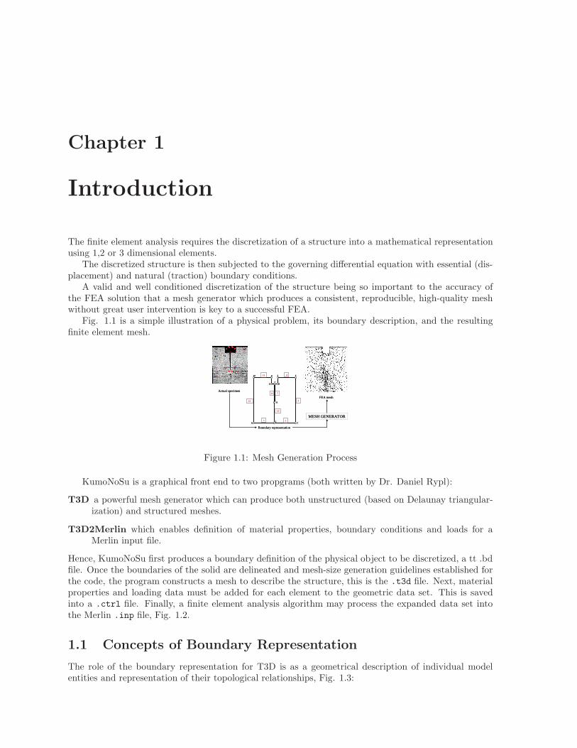
Fig. 1.1 is a simple illustration of a physical problem, its boundary description, and the resultingfinite element mesh.

Actual specimen

Boundary representation

MESH GENERATOR

FEA mesh

1

78 6

5

3

4

2

10

11

9

12

1 2

11 4

3

78

13

Actual specimen

Boundary representation

MESH GENERATOR

FEA mesh

1

78 6

5

3

4

2

10

11

9

12

1 2

11 4

3

78

13

1

78 6

5

3

4

2

10

11

9

12

1 2

11 4

3

78

13

Figure 1.1: Mesh Generation Process

KumoNoSu is a graphical front end to two propgrams (both written by Dr. Daniel Rypl):

T3D a powerful mesh generator which can produce both unstructured (based on Delaunay triangular-ization) and structured meshes.

T3D2Merlin which enables definition of material properties, boundary conditions and loads for aMerlin input file.

Hence, KumoNoSu first produces a boundary definition of the physical object to be discretized, a tt .bdfile. Once the boundaries of the solid are delineated and mesh-size generation guidelines established forthe code, the program constructs a mesh to describe the structure, this is the .t3d file. Next, materialproperties and loading data must be added for each element to the geometric data set. This is savedinto a .ctrl file. Finally, a finite element analysis algorithm may process the expanded data set intothe Merlin .inp file, Fig. 1.2.

1.1 Concepts of Boundary Representation

The role of the boundary representation for T3D is as a geometrical description of individual modelentities and representation of their topological relationships, Fig. 1.3:

1.1 Concepts of Boundary Representation 13

Figure 1.2: KumoNoSu ’s File Types

VERTICES

P� P�P� P� LINEAR CURVE

P� P�P� P� PATCH

P� P�P�

P�P� P�P�

P�RATIONAL BEZIER CURVE

P� P�P�P�P� P�P�

P� RATIONAL BEZIER SURFACE

P�P�

P�P�P�

P�P�P�

Figure 1.3: Entities Recognized by KumoNoSu

Vertices points in (x,y,z) space.

Curves defined by 2 end vertices, may be linear, quadratic, or cubic.

Patches planar collection of curves.

Surfaces non-planar, defined by (4) curves.

Shells non-planar collection of curves.

Regions set of non-self-intersecting boundary surfaces, patches, and shells.

1.1.1 Hierarchy

Those entities are defined hierarchically, Fig. 1.4 Lower level entities which belong to higher level entitiesare called the Minor entities of that higher level entity. Hence:

• Vertices are the minor entities of curves.

• Vertices and curves are the minor entities of patches and surfaces.

• Vertices, curves, surfaces, and patches are the minor entities of regions.


1.2 Kumo Layout 14

Figure 1.4: Hierarchy of Model Representation

1.1.2 Mesh Size/Density

In the process of generating a finite element mesh, it is highly desirable that one can control the meshgradation or density. Hence, wherever the strain energy gradient is highest (such as in zones of stressconcentration), we have a refined mesh. For unstructured meshes, this can be controlled by the size ofan entity for triangular (2D) or tetrahedral (3D) meshes. In Fig. 1.5 we note how the reduction of thesize parameter results in denser uniform mesh over the entire patch.

Figure 1.5: Concept of Mesh Size

For structured meshes, composed of quadrilaterals in 2D or hexagonal in 3D, mesh density can becontrolled by the count concept, Fig. 1.6.

Figure 1.6: Concept of Mesh Count

Finally, gradation of the mesh can be accomplished by assigning different sizes to different entities(small size in the areas of denser mesh, larger size in areas of coarser mesh), Fig. 1.7.

1.2 Kumo Layout

KumoNoSu toolbars has the following main components, Fig. 1.9:

File Controls input/output with external files, Fig. 2.1. This is defined in described in 2


1.2 Kumo Layout 15

Figure 1.7: Concept of Mesh Size; Curve and Patch

Vertex 1 factor 0.1Curve 4 factor 0.1

Vertex 1 factor 0.1Vertex 1 factor 0.1Curve 4 factor 0.1Curve 4 factor 0.1

Figure 1.8: Concept of Factor

Define Boundary Allows user to define the boundary representation of the structure to be meshed,Chapter 3.

View Controls a number of viewing parameters, Chapter 4.2.

Generate Mesh to instruct T3D to generate the finite element mesh using the previously defined .bd

file, Chapter ??.

T3D2Merlin As the main interface which allows definition of the material properties, loads, boundaryconditions, Chapter 6.

Help For setup and info about the code.

Figure 1.9: KumonoSu Toolbar

each one of them will be described in a separate chapter.


Chapter 2

File

The user clicks the file menu to initiate file management, Fig. 2.1 If the session is the initial session for

Figure 2.1: File Management

the project, there is no need to select the File task.

New Wipes out the memory, and enable the definition of a new bd file.

Open bd file If the user has previously created a boundary file and wishes to run another trial usingthe same boundary, the user should Open boundary file. KumoNoSu will present the user withthe available .bd-files stored in the default directory. Even if stored in directories other than thedefault directory, other .bd-files are available by directory search, Fig. 2.2.

Open t3d file This will allow the user to open an existing mesh generated by t3d. The user may notmodify the mesh defined in this file.

Open ctrl file This file contains the load and material properties information used by T3d2Merlin togenerate a Merlin.inp file.

Open inp file to retrieve a Merlin file. There are few instances where this is needed.

Open Parallel input file Eanables the user to select one of the multiple files previously generated byKumoNoSu through its domain decomposition algortihm.

Open b2k file Opens a file coming from Beaver.

Import dxf file Import a dxf file (AutoCad). KumoNoSu will attempt to map vertices and curves.Surfaces and Regions (3D entities) are not recognized by KumoNoSu and will have to be manuallydefined.

Save bd file Once the boundary has been named, the user may save the entity at any phase of devel-opment.

17

Figure 2.2: File Retrieval

Save bd file as Save a bd file for the first time, or with a new name.

Export Will create an .eps, .emf, .jpg, .bmp or .gif file out of the current main window display.

Switch to Cracker which enables the automatic simulation of crack propagation in 2D only


Chapter 3

Define Boundary

The Define Boundary module enables the user to define all the entities which describe the boundary ofthe structure to be discritized. Note this section deals only with the geometric definition of the structure,loads, material properties will be specified later.

This module, Fig. 3.1 will generate a .bd file which in turn will be executed by the T3D module(developed by Daniel Rypl).

Figure 3.1: Boundary Definition Menu

Vertex to define individual points (called vertices), Sect. 3.1.

Curves are one dimensional curves (or lines) connecting vertices, Sect. 3.2.

Patch Define planar entities composed of 3 or more curves, Sect. 3.3.

Surfaces Define non planar entities composed of 3 or 4 curves, Sect. 3.4.

Regions which are three dimensional objects defined in terms of patches or region, Sect. 3.5.

Entity Groups To lump together various basic entities for easier reference later (such assign a tractionto multiple patches), Sect. 3.6.

Mouse Vertex Creation Using a background grid, define vertices with the mouse, Sect. 3.7.

Mouse Curve Creation Using existing vertices, define new curves, Sect. 3.8.

Master/Slave: to tie force entities (vertices, curves, patches or surfaces) to have identical displace-ments, Sect. 3.11.

Embedded Reinforcement to define steel reinforcement perfectly bonded to the surrounded contin-uum, Sect. 3.12.

3.1 Vertex 19

Crack Segments can be line or surface discontinuities, with or without interface elements, Sect. 3.13.1.

Discrete Cracks Define crack entities from previously defined crack segments, Sect. 3.13.2.

Crack Bridging If a reinforcement crosses a crack, Sect. 3.14.

Crack Library (not yet implemented)

Elastic Boundary To apply elastic springs at a vertex, along a curve, or on a patch/surface, Sect.3.16.

Viscous Boundary To apply a nodal or continuum dashpot at a vertex, along a curve, or on apatch/surface, Sect. 3.17.

Zangaar/Westergaard Lumped Mass To determine and apply added masses along a curve or on apatch/surface, Sect. 3.18.1.

Ordinary Lumped Mass Manually defined, Sect. 3.18.2.

Extrude to 3D To extrude a two dimensional mesh into a three dimensional one, Fig. 3.19.

3.1 Vertex

To define a vertex, the user must specify a vertex number (note vertex numbers need not be sequentiallynumbered).

To edit an existing vertex, its id must be entered, and then user must click on Edit, Fig. 3.2.

Figure 3.2: Vertex Definition

Mandatory information for vertices:

Vertex id Not necessarily sequential.

Coordinates Vertex coordinates are entered (for a two-dimensional model, the z-coordinate field is leftblank) in the grid table.

Optional information:


3.2 Curve 20

Size The Size field allows the user to specify a dimension to elements in the vicinity of the vertex. TheSize assigned to a vertex takes precedence over the Size assigned during patch definition (discussedlater). This value can be left blank/zero.

Coincide Vertex Define the vertex number that is coincident with the current vertex. This optionis most often associated with crack definition. Note that if two (or more) vertices have the samecoordinates, the vertices with higher numbers are coincident to the vertex with the lowest number.A coincident vertex should have been previously defined.

Factor is a mesh size multiplying factor (default is one, even if the table shows zero) applied to the -d

value defined as default for the T3D mesh generator. Hence, whereas Size specifies an absolutesize for the mesh (irrespective of the -d value defined later), Factor is relative to that value.

Fixed to Curve Curve number that the vertex is fixed to. If a vertex is to be located on a curve,but not part of the connectivity of that curve, it is fixed to the curve. It should be noted that bydefault a vertex fixed to a parent entity inherits mesh size from that entity.

Control keys:

Apply will accept all changes.

New Vertex will generate a new blank row for data entry.

Delete Vertex will delete that entity. Careful, user must check if this vertex is not used in a curve.

Rename a vertex Allows the user to assign a new vertex id. Kumo will inform user if that vertex isused by curves, Fig. 3.3.

Figure 3.3: Vertex Rename Warning

Close will simply close the current GUI.

Note:

1. Table can be sorted in ascending/descending order of any of the column values, Fig. 3.4.

2. Dulicate vertex numbers are highlighted.

3. the “smiley” icon means that the vertex is used (at least once) in a curve definition. whereas the“sad” icon means that the vertex is an “orphan” and is not referenced by any curve. (This mayhappen if the vertex is Fixed on a curve or patch, and is used to have its displacements monitored).

4. User can use the usual Ctrl-C and Ctrl-V to copy and paste into the matrix.

3.2 Curve

Curve is a compulsory keyword. Mandatory information for all curves, Fig. 3.5: Fig. 3.5.

Curve id : Required for patch, surface, and shell definitions; does not have to be sequential.


3.2 Curve 21

Figure 3.4: Vertex Reorder/Duplicate Warning

Figure 3.5: Curve Definition


3.2 Curve 22

from-to : Curve start and end vertex numbers (The direction of the curve is from the Vertex i to Vertexj). While the user may assign any direction to the curve, he would be well advised to utilize aconvention that facilitates COUNTER-CLOCKWISE element (a patch in two-dimension models)construction.

Optional information

Size The Size field allows the user to specify a dimension to elements in the vicinity of the curve. TheSize assigned to a curve takes precedence over the Size assigned during patch definition (discussedlater). This value can be left blank/zero.

Factor is a mesh size multiplying factor (default is one, even if the table shows zero) applied to the -d

value defined as default for the T3D mesh generator. Hence, whereas Size specifies an absolutesize for the mesh (irrespective of the -d value defined later), Factor is relative to that value.

Coincide Defines a curve number that is coincident with the current curve. This option is most oftenassociated with crack definition. Note that if two (or more) curves have the same coordinates, thecurve with higher id is coincident to the curve with the lower id. A coincident curve should havebeen previously defined.

Count : Define number of quad/hexa elements along the curve (for structured mesh only).

Duplicate : Define that the mesh nodes along this curve must duplicate those of the specified curve.

Curve order : Linear (order 2, default), Quadratic (order 3), Cubic (order 4). Circular, parabolic,hyperbolic and elliptical curves can be defined with curves of order 3 and 4; though the fourthorder should used preferably.

1D element : Specify that this curve is to be included in the mesh as a 1D element. 1D elements(typically steel reinforcement) requires a material ID, specified in the Material ID box.

Control keys:


New Curve will generate a new blank row for data entry.

Delete Curve will delete that entity. Prior to deleting, KumoNoSu will check if this curve is not usedsubsequently, 3.6

Figure 3.6: Curve Delete Warning

Rename Curve Allows the user to assign a new vertex id. Kumo will inform user if that curve id isalready used, Fig. 3.7.

Figure 3.7: Curve Rename Warning



3.2 Curve 23

3.2.1 Higher Order Curves

T3D (and thus KumoNoSu ) uses rational Bezier curves1 which are described in details in chapter BWhen higher order curves (such as quadratic or cubic) are to be specified a second dialog appears

for further definition of control points for the nonlinear curve, KumoNoSu will automatically calculatethe control points for (4) types of curves:

Circular arcs : User must specify the center coordinates of the arc, and indicate if the arc is smalleror greater than 180o. Note that vertices i and j would have been defined in the previous dialogbox, Fig. 3.8.

If all three points lie on a straight line, then the arc sustains an angle of 180o, and then a directionvector (Vx, Vy , [Vz]) defines the direction from the circle origin through the center of the arc.

vertex i

vertex j

(c�,c�,c�) vertex i

vertex j

(c�,c�,c�)vertex ivertex j

(c�,c,c)(v�,v,v)

vertex ivertex j(c�,c,c)

(v�,v,v)Figure 3.8: Circular Curve Definition

Elliptical arcs : Defined by the coordinates of the ellipse center (cx, cy, [cz]), a and b and the directionvector (Vx, Vy, [Vz ]) from the center to the center of the arc. Note that vertices i and j would havebeen defined in the previous dialog box, Fig. 3.9.

1Rypl, D., T3D, Triangularization of 3D Domains, User Guide, January 2001.


3.3 Patch 24

vertex i(c�,c�,c )(v�,v�,v )

vertex ja

bvertex i

(c�,c�,c )(v�,v�,v )

vertex ja

b

Figure 3.9: Elliptical Curve Definition

Parabolic arcs : The parabola is completely defined by the two vertices i and j (defined in the previousdialogue box), and the parabola vertex cx, cy, [cz]), Fig. 3.10.

Hyperbolic arcs : The hyperbola requires definition of a and b as well as a direction vector (Vx, Vy, [Vz ]).Note that vertices i and j would have been defined in the previous dialog box, Fig. 3.11.

Additionally, control points and weights may be defined by the user.For subsequent editing of the curve parameters, user should double click on the curve id. Note that

if a curve is not linear, the smiley/sad face would have a different color.

3.3 Patch

A patch is a two dimensional section in a plane. A patch can be defined by multiple curves, however allthose curves must be co-planar (if not an unforseen error may occur).

During Patch definition, the direction of the defined members is critical. This direction must becounterclockwise with respect to the normal vector (automatically determined by KumoNoSu ), andpointing outward.

If the curve definition (from i to j vertex) follows the counter-clockwise orientation, it is consideredpositive in the boundary curve definition. If the curve definition is oriented clockwise, it is considerednegative in the boundary curve definition, Fig. 3.12. Once the data has been accurately added oradjusted for a patch, the user selects the Accept option from the Patch Control sub-menu. Once allvertex data has been entered accurately, the user selects the Save patches button at the bottom of thePatch menu-board.

Mandatory information for all patches, Fig. 3.13: Fig. 3.5:

Patch id number Required for reference in 2D; required for region definitions in 3D; does not have tobe sequential.

Boundary curves List of curves completely defining the patch.


3.3 Patch 25

Figure 3.10: Parabolic Curve Definition

vertex i vertex j

a

b•Intersection point for 2 hyperbola tangent lines

(v�,v�,v�)•a,b: distances from hyperbola max/min point to the intersection point for the hyperbola tangent lines

vertex i vertex j

a

b•Intersection point for 2 hyperbola tangent lines

(v�,v�,v�)•a,b: distances from hyperbola max/min point to the intersection point for the hyperbola tangent lines

Figure 3.11: Hyperbola Curve Definition


3.3 Patch 26

+

1

7

6

5 43

2

8

9

10

+4

++

1

7

6

5 43

2

8

9

10

++4

Figure 3.12: Counter-Clockwise Patch Definition

Figure 3.13: Patch Definition

Material Material number associated with the current patch (only for 2D models). Material numbermust be assigned to two-dimensional patches. The material properties associated with the Materialnumber are defined later from the T3D2Merlin pull-down menu using the Element Groups menu.

Optional selections:

Size Defines mesh size for a patch. The Size field for a patch defines the strong dimension of elementswithin the vicinity of the patch. The Size assigned within the Patch definition menu is weakerthan the previous two Size definitions and always defers to previous definition.

Coincide Defines patch number that is coincident with the current patch. For crack modeling in three-dimensional space, Coincide Patch defines the two surfaces initially occupying the same space.

Hole Defines that this patch is a hole (it will not contain a mesh). This is used for inserting holes inlarger patches.

Additional optional parameters may be entered by double clicking on the patch id:

Factor Defines patch mesh size multiplication factor.

Fixed Vertices Defines vertex id of those vertices which lie inside the patch (if any exist).

Fixed Curves Defines curve id of those curves which lie inside the patch (if any exist).

Subpatches Defines the patch numbers of those patches which lie completely inside the patch. Forexample, hole patches are subpatches (they are inside larger patches).

Boundary curves No. 2 Defines a second set of boundary curves (used for special circumstancesonly).

Control keys:


3.4 Surface 27


New patch will generate a new blank row for data entry.

Delete patch will delete that entity. Prior to deleting, KumoNoSu will check if this curve is not usedsubsequently, 3.14

Figure 3.14: Patch Delete Warning

Rename Curve Allows the user to assign a new patch id. Kumo will inform user if that curve id isalready used.


Max Curves Allows the user to increase the number of allowable curves which define a patch. Careful,if you decrease the current number, you may lose data associated with patch having a large numberof curves.

3.4 Surface

A surface is bound by three or four curves (not necessarily coplanar) defined sequentially (i.e. each curvemust be connected to the previously defined one, and the one defined after it).

Curves are specified as positive integers, i.e. we need not worry about continuity of the curves for thesurface definition Surface is positive if curves are ordered clockwise around the outer side of the surface.

Curve order in the surface definition matters. Curve direction does not matter.When defining a region, a surface id may be +ve (if its outward direction is pointing out), or ve (if

its outward direction is pointing inside).Surfaces are only applicable to 3D boundary descriptions, Fig. 3.15.

Figure 3.15: Surface Definition

Input data for the Surfaces, are of two types:

Mandatory for all surfaces:

Surface id Required for region definitions in 3D; does not have to be sequential.

Surface curves Three or four curves which define the four sides of the surface. At least one ofthese curves must be nonlinear, else the surface is planar and is a patch.

Optional


3.5 Region 28

Size Defines mesh size for the surface.

Factor Defines surface mesh size multiplication factor.

Coincide Defines surface number that is coincident with the current surface.

In certain instances, polygon control information will be required for the surface, in which case a seconddialog box will open for this information.

It should be noted that the order of the four curves which compose the surface is dependent upon theouter side of the surface (i.e. the side that defines the exterior of the model. Hence, curves are orderedclockwise around the outer side of the surface, and the following rules apply, Fig. 3.16.


1. If only 1 or 2 nonconsecutive curves in a surface are order 3, do not specify a polygon for thesurface.

2. If 2 or more consecutive curves in a surface are order 3, a polygon must be specified for thesurface.

3. If only 1 or 2 nonconsecutive curves in a surface are order 4, do not specify a polygon for thesurface.

4. If 2 or more consecutive curves in a surface are order 4, four polygon coordinates must be specifiedfor the surface.

5. If 1 curve is order 3, and the previous or subsequent curve is order 4, two polygon coordinatesmust be specified.

When defining cracks, bounded by two adjacent surfaces then: The two surfaces must be identicallydefined, i.e the first vertex of the first curve must have the same coordinates for both surfaces, Fig. 3.17.

3.5 Region

In three-dimensional models the regions must be defined. A region defines a volume. Just as curvescomprise boundaries define patches, patches and/or surfaces combine to define the boundaries of a region.

For a region, a patch is defined as positive if its normal points in a positive direction, as defined bythe global coordinates. A negative sign during the Boundary patch definition must precede any patchthat has a negative unit normal.

The Size defined in the Region definitions is weaker still than the Size defined in the Patch definitions.The user edits regions in a similar fashion as vertices and patches: insert the appropriate number anddouble click the field box.

Mandatory input parameters for all regions: 3.18.

Region id For reference; does not have to be sequential.


3.5 Region 29

Curves11: 2 3 43: 1 515: 3 7 35: 5 623: 9 7 37: 8 617: 2 9 82: 1 8

Surfaces1: 11 17 23 152: 43 82 37 35

Regions1: … 1 ….2: … -2 ….

1115

2317

4335

3782

1

5 6

8

2

37

9

1

2

Curves11: 2 3 43: 1 515: 3 7 35: 5 623: 9 7 37: 8 617: 2 9 82: 1 8

Surfaces1: 11 17 23 152: 43 82 37 35

Regions1: … 1 ….2: … -2 ….

1115

2317

4335

3782

1

5 6

8

2

37

9

1

2

1115

2317

4335

3782

1

5 6

8

2

37

9

1

2

Figure 3.17: Surface Crack Definition



3.5 Region 30

Material Material number associated with the current region.

Hexahedral User may specify if the elements to be generated in the current regions are Tetrahedrons(default), Hexahedral, or a combination of the two.

Boundary patches List of patches composing the boundary of the region (if any exist.

Boundary surfaces List of surfaces composing the boundary of the region (if any exist).

Optional entries are

Size Define mesh size for the region.

Factor Define region mesh size multiplication factor.

Fixed curves Define any curves which lie inside the region and are not connected to any patch orsurface.

Hole Indicating that we have a three-dimensional cavity.

Control keys:


New Region will generate a new blank row for data entry.

Delete Region will delete that entity. Prior to deleting, KumoNoSu will provide the user with a list ofall entities pertaining to this region, 3.19. The user can then delete all those entitities, or uncheckthose which should be retained.

Figure 3.19: Region Delete Warning

Rename Allows the user to assign a new patch id. Kumo will inform user if that curve id is alreadyused.


Max Patches/Surfaces Allows the user to increase the number of allowable patches/surfaces whichdefine a patch. Careful, if you decrease the current number, you may lose data associated withpatch having a large number of curves.

Certain important rules apply for region definition, Fig. 3.20:

1. Boundary surface numbers are always positive.

2. Boundary patch numbers are positive if the patchs normal points OUT of the region.

3. Boundary patch numbers are negative if the patchs normal points INTO the region.

4. Since the surface normal (defined by the order of the surface curves) is always out of the region,boundary surface numbers are always positive.


3.6 Entity Groups 31

XZ

Y

1

7

56

4 2

3

8

8

7

4

12 10

9

11

5

1

2

6

3

1

3 2

4

6

5

XZ

Y

1

7

56

4 2

3

8

8

7

4

12 10

9

11

5

1

2

6

3

1

3 2

4

6

5

Figure 3.20: Region Definition

3.6 Entity Groups

NEED TO FIX KUMO Entity groups enable the user to lump or group together various entities whcihwill subsequently inherit the same characteristic (particularly in the load definition).

3.7 Mouse Vertex Creation

User can use the mouse to define new vertices and have them connected by curves, Fig. 3.21. However,user must first select a projection plane, and then specify the third coordinate through the slider. Atthat point, when the left button of the mouse is pressed a new vertex is created at the closest grid point.Grid resolution must be defined within the View Option in Section 4.1.5. Note that the mouse currentposition is echoed in the bottom toolbar. If Enable Point Creation is active, then pressing the mousecreates the new vertex. If Connect Points with Curves is active, then sequential curves are defined.

Figure 3.21: Vertex Definition by the Mouse

3.8 Mouse Curve Creation

This option, Fig. 3.22 enables the user to select individual vertices with the mouse and have themconnected by curves.


3.9 Curve Selection 32

Figure 3.22: Curve Definition by the Mouse

3.9 Curve Selection

This option, Fig. 3.23 enables the user to select curves by clicking the curve number with the left buttonof the mouse. Once selected, the curve is assigned a new color. The list of curves is first saved in a bufferinside the dialogue box.

It is important to note that the first curve selected should be oriented in a counterclockwise directionfor the patch to be selected (i.e. it will be defined as a positive integer in the patch definition).

To deactivate a selection, user must click again on a previously selected curve.When the user selects Create a new patch is created with the selected curves. Kumo will attempt to

determine the sign of the curve id’s (based on the first one defined) such that a counterclockwise patchis defined.

User should open the patch definition menu, and assign to the newly created patch the properparameters (such as material group if 2D analysis).

Figure 3.23: Curve Selection with the Mouse

3.10 Patch/Surface Selection

This option, Fig. 3.24 enables the user to select patches by clicking the patch number with the leftbutton of the mouse. The list of patches is first saved in a buffer inside the dialogue box.

A powerful feature, is to automatically add all the patches connected to the previously selected one.User has simply to keep on clicking on Add Face and kumo will identify the adjacent patches connectedto the previously defined one. This process can be repeated recursively.

It is important to note that the first patch selected should have an outward normal.To deactivate a selection, user must click again on a previously selected patch.When the user selects Create a new region is created with the selected patches/surfaces. Kumo will

attempt to determine the sign of the patches/surfaces id’s (based on the first one defined) such that theoutward normal ones have a positive id number.

User should open the region definition menu, and assign to the newly created region the properparameters (such as material group).

3.11 Master/Slave

Master/slave nodes in the FE mesh may be defined in KumoNoSu through the master/slave pair defi-nition dialog. Both vertex pairs and curve pairs may be defined in the dialog. In the case of M/S curve


3.12 Embedded Reinforcement 33

Figure 3.24: Patch/Surface Selection with the Mouse

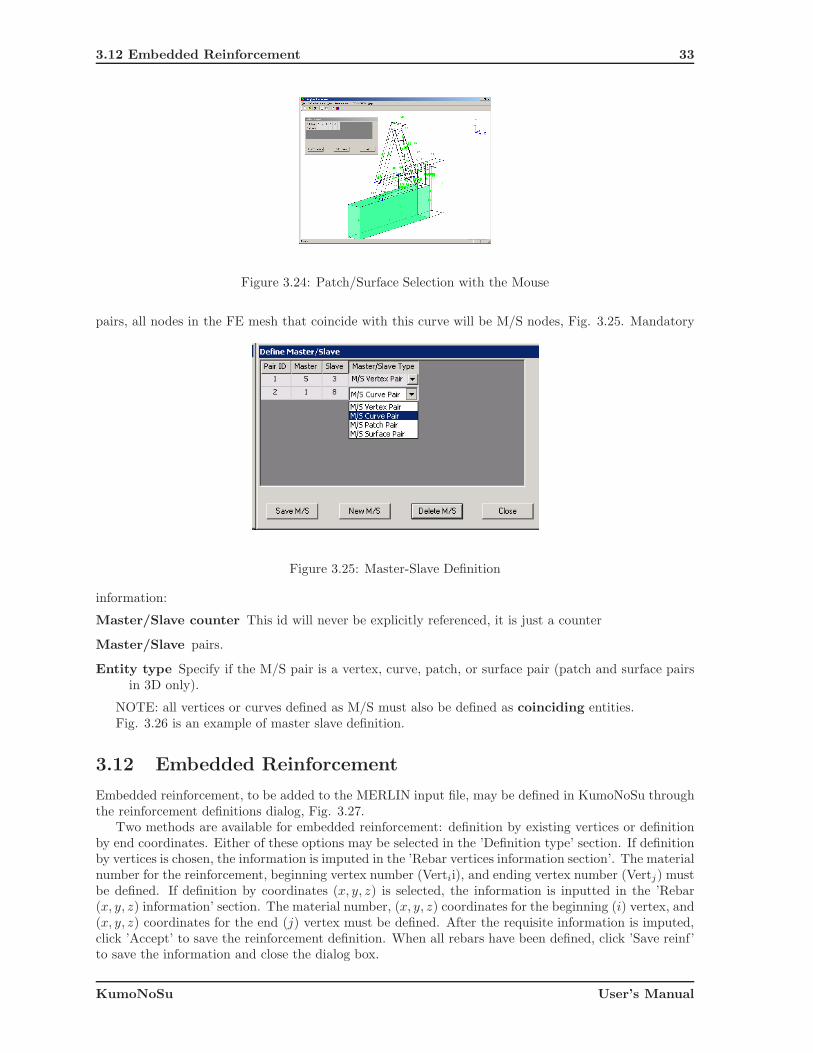
pairs, all nodes in the FE mesh that coincide with this curve will be M/S nodes, Fig. 3.25. Mandatory

Figure 3.25: Master-Slave Definition

information:

Master/Slave counter This id will never be explicitly referenced, it is just a counter

Master/Slave pairs.

Entity type Specify if the M/S pair is a vertex, curve, patch, or surface pair (patch and surface pairsin 3D only).

NOTE: all vertices or curves defined as M/S must also be defined as coinciding entities.Fig. 3.26 is an example of master slave definition.

3.12 Embedded Reinforcement

Embedded reinforcement, to be added to the MERLIN input file, may be defined in KumoNoSu throughthe reinforcement definitions dialog, Fig. 3.27.

Two methods are available for embedded reinforcement: definition by existing vertices or definitionby end coordinates. Either of these options may be selected in the ’Definition type’ section. If definitionby vertices is chosen, the information is imputed in the ’Rebar vertices information section’. The materialnumber for the reinforcement, beginning vertex number (Vertii), and ending vertex number (Vertj) mustbe defined. If definition by coordinates (x, y, z) is selected, the information is inputted in the ’Rebar(x, y, z) information’ section. The material number, (x, y, z) coordinates for the beginning (i) vertex, and(x, y, z) coordinates for the end (j) vertex must be defined. After the requisite information is imputed,click ’Accept’ to save the reinforcement definition. When all rebars have been defined, click ’Save reinf’to save the information and close the dialog box.


3.12 Embedded Reinforcement 34

1

46 3

2

56

7

5 4

3

2

I

9 8

810

9

II

710 11

1

46 3

2

56

7

5 4

3

2

I

21

46 3

2

56

7

5 4

3

2

I

9 8

810

9

II

710 11

1

46 3

2

56

7

5 4

3

2

I

21

46 3

2

56

7

5 4

3

2

I

9 8

810

9

II

710 11

1

46 3

2

56

7

5 4

3

2

I

2

Figure 3.26: Master-Slave Definition Example

Figure 3.27: Embedded Reinforcement


3.13 Cracks 35

3.13 Cracks

3.13.1 Crack Segments

A Crack is composed of one or multiple segments. The first step consists in defining those pairs ofsegments which will later constitute a crack, Fig. 3.28:

Figure 3.28: Crack Definition

Type which can be a curve, patch or surface.

Upper/Lower entities.

Note:

1. Crack paths are always defined from crack front to crack mouth.

2. Curve orientation (i and j vertices) in each segment must be from crack front to crack mouth.

3. The two curves or patches composing each crack segment must be defined as Coincide.

4. 2D Crack segment upper and lower curves are prescribed according to the location of the crackfront and Fig. 3.29.

x

Front

Mouth

UPPER

LOWERx

Front

Mouth

UPPER

LOWER

Figure 3.29: Crack Orientation Definition for 2D Cases

5. 3D Crack segment upper and lower patches are prescribed according to which patch is on top whenthe crack opens (in terms of the positive global coordinate directions), Fig. 3.30.


3.13 Cracks 36

x3

x1

x2

UPPER patch (or surface)

LOWER patch (or surface)

x3

x1

x2

UPPER patch (or surface)

LOWER patch (or surface)

Figure 3.30: Crack Orientation Definition for 3D cases

Figure 3.31: Discrete Crack Definition


3.13 Cracks 37

3.13.2 Discrete Cracks

One the crack segments have been defined, the User may now define the discrete cracks, Fig. 3.31.

Discontinuity id is the id associated with the crack/discontinuity about to be defined.

Discontinuity Option Partially implemented

Insert Interface Spring between the two lips of the discontinuity. Not yet implemented.

Insert Interface Damper between the two lips of the discontinuity. Not yet implemented.

Perform LEFM/NLFM Analysis, is by default the option.

Fracture Analysis Type Linear Elastic Fracture Mechanics (LEFM), Nonlinear Fracture Mechanics(NLFM), or LEFM with interface crack elements (cohesive crack model).

Crack Type Option Interface cracks are between two patches in two-dimensional analyses and be-tween two regions in three-dimensional analyses. A structure crack develops within a patch or aregion.

Discrete Crack Definition

Discrete crack segments lists the crack segments id’s constituting the discrete crack.

Upper crack front curve Vertex (or curve in 3D) at the upper surface crack front.

Lower crack front curve Vertex (or curve in 3D) at the lower surface crack front.

Discrete Crack Mat’l ID to be used only if interface elements are to be inserted along the crack(NLFM or LEFM with ICM options).

Interface spring/damper properties Inactive.

Note that identification of the upper and lower curves is for the proper application of the uplift (FERCmodel).

3.13.3 Examples

Fig. 3.32 is an example of 2D structure crack where the Upper crack surface is curve 6, the lower one is7, the crack front is 7. The crack is defined by only one crack segment.

1 2

6 5

431

MOUTH

FRONT

2

4

7 635 I 7

1 2

6 5

431

MOUTH

FRONT

2

4

7 635 II 7 1 2

6 5

431

MOUTH

FRONT

2

4

7 6

35 I7

UP

PE

RL

OW

ER

1 2

6 5

431

MOUTH

FRONT

2

4

7 6

35 II7

UP

PE

RL

OW

ER

Figure 3.32: 2D Example of a Structure Crack

Fig. 3.33 is an example of 3D structure crack. The crack segment is composed of the pair of patchesI and II, the crack front is defined by curve 5. The upper segment is II (because it is “above” patch I inthe positive X direction), the lower one is I.

A 2D interface crack is shown in Fig. 3.34. Vertex 11, 12, 13 must coincide with vertex 1, 2, 3respectively (Vertex 11, 12, 13 must be defined AFTER vertex 1, 2,3). Curves direction MUST bedefined from tip (or front) to the mouth of the crack Curves 14 and 15 must coincide with curves 4 and5 respectively. (Curves 14 and 15 must be defined AFTER curves 4 and 5.

Another example of 2D interface crack is shown in Fig. 3.35.Fig. 3.36 is an example of 3D interface crack.


3.13 Cracks 38

FRONT

II

I

Z

X

Y

5

FRONT

IIII

II

Z

X

Y

5

FRONT

Z

X

Y

III

5

FRONT

Z

X

Y

III

FRONT

Z

X

Y

IIIIII

5

Figure 3.33: 3D Example of a Structure Crack

x

y1 3

11 12 13

24 5

14 15

FRONT

n

m curve number

vertex number

UPPER

LOWER

MOUTH

x

y1 3

11 12 13

24 5

14 15

x

y1 3

11 12 13

24 5

14 15

FRONT

n

m curve number

vertex number

UPPER

LOWER

MOUTHFRONT

n

m curve number

vertex number

UPPER

LOWER

MOUTH

Figure 3.34: 2D Example of an Interface Crack, Upper and Lower

1 2

8 5

43

7 6

1

MOUTH

FRONT

2

5 4

8 7 36 I II

1 2

8 5

43

7 6

1

MOUTH

FRONT

2

5 4

8 7 36 I II

MOUTH

FRONT

1 2

8 7

1

5

86 I

5

43

6

2

4

7 3II

UPPER

LOWER

MOUTH

FRONT

1 2

8 7

1

5

86 I

1 2

8 7

1

5

86 I

5

43

6

2

4

7 3II

5

43

6

2

4

7 3II

UPPER

LOWER

Figure 3.35: 2D Example of an Interface Crack, Upper and Lower


3.14 Crack Bridging a Truss Element 39

FRONT

II

I

Z

X

Y

56

FRONT

IIII

II

Z

X

Y

56

I

Z

Y 5

REGION 1

X

II

6

REGION 2

I

Z

Y 5

REGION 1

II

Z

Y 5

REGION 1

X

II

6

REGION 2

X

IIII

6

REGION 2

Figure 3.36: 3D Example of an Interface Crack

3.14 Crack Bridging a Truss Element

In reinforced concrete analysis, a crack may cross a truss element modeling a rebar, Fig. 3.37.

Figure 3.37: Rebar Crossing a Crack

Case No. For reference; does not have to be sequential.

Upper vertex Vertex number of the curve end which lies on the upper surface of the crack.

Lower vertex Vertex number of the curve end which lies on the lower surface of the crack

Fig. 3.38 is a simple illustrative example.

3.15 Crack Library

Inactive


3.16 Elastic Boundary 40

Figure 3.38: Example of Rebar Crossing a Crack

3.16 Elastic Boundary

Elastic Boundary enables the user to specify elastic springs along a global direction (X , Y or Z) on avertex, along a curve or over a patch.

The spring stiffness can be determined either from

K =AE

t(3.1)

where A is the tributary area of the spring (automatically determined by KumoNoSu ) on the basisof adjacent elements, E is the Young’s modulus of the adjoining material (automatically detected byKumoNoSu ), and t is the effective thickness to be specified by the user, or can be explicitly given, Fig.3.39.

Figure 3.39: Elastic Boundary

User is reminded that the spring connects an entity to a rigid support.

3.17 Viscous Boundary

3.17.1 Discrete Dashpots/Nodal

3.17.2 Continuous Dashpots/Elements

Viscous boundaries absorbs the energy from pressure and shear waves, (?). Damping of these waves isbased upon the elastic properties of the continuum along the boundary

C = ρViA

{

Shear Wave: Vs =√

Gρ

Pressure Wave: Vp = 1sVs; s

2 = 1−2ν2(1−ν)

(3.2)

Mandatory information for all viscous boundaries, Fig.3.40


3.18 Lumped Masses 41

Figure 3.40: Viscous Boundary

B.C id boundary condition number, for reference.

Formulation Interface continuum will generate continuum dashpots elements along the selected entity.In 2D these will be four noded elements, and in 3D 6 or 8 noded elements.

Entity type (curve in 2D, patch or surface in 3D).

Interface Continuum parameters

Entity No. to identify the curve, patch or surface.

Mat ID Material group associated with the viscous interface elements (to be defined later).

Offset Distance The interface dashpot elements have a zero thickness formulation. Hence, usercan select an arbitrary offset distance for visualization.

Nodal Discrete parameters

Entity No. number of the entity at which to apply viscous B.C.s.

Mass density mass density γ of the material on the viscous boundary (if zero or blank, the γ ofthe actual material will be used).

X-dir, Y-dir, [Z-dir ] degree of freedom to be damped.

Damp pressure wave/Damp shear wave wave to be damped.

3.18 Lumped Masses

3.18.1 Westergaard-Zangaar

Mandatory information for all Westergaard (vertical upstream face) or Zangaar (inclined upstream face)added mass, Fig.3.41


3.18 Lumped Masses 42

Figure 3.41: Westergaard Added Mass Definition

Nodal mass number for reference.

Lumped Mass type Westergaard or Zangar.

Entity type Curve (in 2D) or Patch (in 3D).

Entity No. entity number.

Axis defining reservoir depth X , Y (or Z in 3D).

K constant K constant for Westergaard equation (defined by Westergaard as 51.0 lb/ft3 or 8011.4N/m3).

Water elevation Elevation of the reservoir surface (note that this is not the relative depth of thereservoir, but rather the elevation of the surface).

Water modulus Elastic modulus of the water (may be taken as 300 kips/in2 or 2.068 GPa).

Fluid weight weight per unit volume of the fluid (Westergaard only).

Accel of gravity Acceleration of gravity.

Quake period Period of the earthquake motion (Westergaard only).

Relative fluid depth Relative depth of the reservoir.

3.18.2 User-Defined

This feature must be checked.


3.19 Extrude 43

Figure 3.42: Lumped Mass Definition

3.19 Extrude

The extrude capability, Fig. 3.43 enables the user to begin with a 2D mesh definition, and then extrudeit into a 3D mesh along the z axis by a user specified length.

Figure 3.43: Extrude Interface


Chapter 4

View

4.1 View Settings

4.1.1 Viewer Config

Fig. 4.1...

Figure 4.1: Viewer Configuration

4.1.2 Selective Display

Fig. 4.2 ....

Figure 4.2: Selective Display

4.1 View Settings 45

4.1.3 Domain Display

Fig. 4.3 ...

Figure 4.3: Domain Display

4.1.4 Load Display

Fig. 4.4 ....

Figure 4.4: Load Display

4.1.5 Creation Control

Fig. 4.5 ....


4.2 Kumonosu Settings 46

Figure 4.5: Creation Control

4.2 Kumonosu Settings

4.3 Settings

The user may wish to set or adjust the Preprocessor settings, Fig. 4.6. This enables the user to specify:

Figure 4.6: KumoNoSu Setting

1. Paths where the supporting software resides (T3d, T3d2Merlin, Acrobat Reader and Gnuplot).

2. Colors of various entities used by KumoNoSu .

4.4 Lighting

Fig. 4.8 ...

4.5 Reset Camera


4.5 Reset Camera 47

Figure 4.7: Kumonosu Settings

Figure 4.8: Light Settings


Chapter 5

Generate Mesh

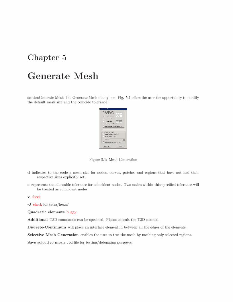
sectionGenerate Mesh The Generate Mesh dialog box, Fig. 5.1 offers the user the opportunity to modifythe default mesh size and the coincide tolerance.

Figure 5.1: Mesh Generation

d indicates to the code a mesh size for nodes, curves, patches and regions that have not had theirrespective sizes explicitly set.

e represents the allowable tolerance for coincident nodes. Two nodes within this specified tolerance willbe treated as coincident nodes.

v check

-J check for tetra/hexa?

Quadratic elements buggy

Additional T3D commands can be specified. Please consult the T3D manual.

Discrete-Continuum will place an interface element in between all the edges of the elements.

Selective Mesh Generation enables the user to test the mesh by meshing only selected regions.

Save selective mesh .bd file for testing/debugging purposes.

Chapter 6

T3D2MERLIN

After successful generation of the mesh by T3d (.t3d file), the user must first define a control file (.ctrl)and then run T3d2Merlin to create a Merlin input file. All of the information required by the controlfile may be defined from the T3d2Merlin pull-down menu. The menu, Fig. 6.1 lists:

Figure 6.1: T3D2Merlin Menu

Title Sect. 6.1.

Keyword to specify the control commands, Sect. 6.2.

Material/Element Groups For material definition, Sect. 6.3.

AAR Properties Sect. 6.4.

Discrete/Continuum Groups To enable the generation mesh with interface elements in between allthe elements, Sect. 6.5.

Eigenmode Analysis Sect. 6.6.

Loads Definition Sect. 6.7.

Incremental Material Update to modify material properties within load increments, Sect. 6.8.

Generate Free Field for dynamic analysis with radiation damping and active free field, Sect. 6.9.

Run Free Field Perform the finite element analysis of the free fields, and define the boundary condi-tions for the mesh, Sect. 6.10.

Write .ctrl File Save the cntrol file, Sect. 6.11.

Generate Merlin .inp file , Sect. 6.12

6.1 Title 50

6.1 Title

The user may provide a description the contents of the input file within this field. This line will bewritten verbatim into the beginning of the Merlin input file, Fig. 6.2.

Figure 6.2: Title Data Entry

It is strongly recommended to include the selected units in the Title.

6.2 Keywords

The Keywords-menu allows the user to define general control options for the subsequent Merlin analysis,Fig. 6.3.

Figure 6.3: Keywords Specification

6.2.1 General options

6.2.1.1 Monitor Max/Min StressMerlin:??Specify which maximum stress component is to be monitored throughout the analysis and its maximum

reported (and corresponding location) reported for each increment.

6.2.1.2 AutoCrackMerlin:1.1.12This keyword is associated with the module Cracker which drives Merlin for automatic crack propagation.

When Merlin senses that either a crack is to nucleate, or a crack must extend, thus requiring remeshingto accomodate discrete cracks, then control is passed back from Merlin to Cracker, Fig. 6.5.


6.2 Keywords 51

Figure 6.4: Monitor Maximum Stress

Figure 6.5: Auto-Crack Specification

Automatic Propagation Allows merlin to remesh if a crack wants to propagate. The user can specifythe number of instances that crack stability requirements have been violated before remeshingtakes place. Violation occurs if the stress intensity factor exceeds the fracture toughness in LEFM,or if the crack tip tensile stress exceeds the tensile strength of the material in NLFM.

Automatic Crack Nucleation Allows Merlin to interrupt the analysis if at some points the maximumtensile principal stress exceeds the tensile strength. If desired, the user can specify boxes insidewhich no crack nucleation can take place.

Automatic Crack Branching Will allow crack bifurcation.

6.2.1.3 MultLDCurvesMerlin:1.1.11.2This option will allow the user to track the load displacement response of a set of nodes, Fig. 6.6.

As data entry for this option can be confusing, the user should understand that:

1. One or more curves can be specified.

2. Each curve will allow the user to specify load and displacement.

3. The displacement can be either one of a specific node/dof, or the algebraic sum of multiple node/dofpairs. This is important if one needs a crack opening displacement (then one facor would be +1,and the other -1), or the displacement of a point with respect to the base. This corresponds to theDisp. #.

4. The load can be either the load at one vertex, or the entire load applied along a curve or over apatch. Again, at time one may need the resultant of a traction load.

Disp # or Load # Number of the current displacement or load monitoring point (for reference).

Entity type type of entity at which to monitor loads or displacements (vertex, curve, or patch).

LD Curve # Curve number that the current displacement or load monitoring point belongs to.


6.2 Keywords 52

Figure 6.6: Load Displacement Curve Definition

Entity # number of the current entity.

dof degree of freedom to monitor (1-2-3).

fact Factor to be applied to the displacement (note, factors are only defined for displacements).

6.2.1.4 TimeAccelCurve

A single time-acceleration curve may monitor the accelerations vs. time (or increments) at one or morevertices, 6.7:

Figure 6.7: Time Acceleration Curve Definition

Case # Number of the current monitoring point (for reference).

Curve Title to identify it amongst other plots.

TA Curve # Curve number that the current monitoring point belongs to.

Vertex # Vertex number of the current monitoring point.

dof Degree of freedom to monitor (acceleration).

compoment Stress component to monitor.

fact Factor to be applied to the acceleration/displacement/stress at the current monitoring point.


6.2 Keywords 53

6.2.1.5 TimeDispCurveMerlin:1.1.11.3Definition of one or more time-displacement is performed using the Define time-displacement parameters

dialogs, 6.8:

Figure 6.8: Time Displacement Curve Definition


Title to be assigned to the curve.



dof Degree of freedom to monitor.

fact Factor to be applied to the displacement at the current monitoring point.

6.2.1.6 Time Stress CurveMerlin:1.1.11.6Definition of one or more time-stress is performed using the Define time-stress parameters dialogs, 6.9,

(TimeStrsCrv option in Merlin):

Figure 6.9: Time Stress Curve Definition



6.2 Keywords 54




component Stress component to monitor.

fact Factor to be applied to the acceleration/displacement/stress at the current monitoring point (maybe useful to convert units).

6.2.1.7 Time Strain Curve

Definition of one or more time-strain is performed using the Define time-strain parameters dialogs, 6.10,(TimeStrnCrv option in Merlin):

Figure 6.10: Time Strain Curve Definition





component Stress component to monitor.

fact Factor to be applied to the acceleration/displacement/strain at the current monitoring point (maybe useful to convert units).

6.2.1.8 UserCurvesMerlin:1.1.7In various instances of Merlin, User may define specific x-y curves (such as for GF , Dynamic uplift etc).

This option enables the user to explicitly specify one or more curve, which will then be referenced in theinput data.

6.11

Figure 6.11: User Defined Curve

6.2.1.9 BandwidthMin

This is an optional setting that allows the user to minimize the time Merlin spends decomposing theglobal stiffness matrix.


6.2 Keywords 55

6.2.1.10 RealTimeViewMerlin:1.1.13Requests the generation of an external file containing the displacements and accelerations at selected

nodes every n increments. Merlin will then generate an .rtv file for real time view during the analysisby Spider.

6.2.1.11 Restart on IncrementMerlin:1.1.3This option enables Merlin to use the previously generated .pst file to restart at a certain increment.

This is most useful when first a static analysis is performed, followed by a dynamic one.

6.2.1.12 Do Not Write Mesh

This option specifies that for the current Merlin input file, there is no need to write the mesh data, asthose may be coming from the restart file.

6.2.1.13 InitAnalflag

Missing

6.2.1.14 Split OutputMerlin:1.7.21In some analysis, the ASCII output file may be too large for the operating system or for the editor. This

option enables the user to split the output into multiple files, each containing the results of n increments.

6.2.1.15 Split .pst

In some analysis, the .pst output file may be too large for the operating system. This option enables theuser to split the .pst file into multiple files, each containing the results of n increments.

6.2.1.16 Initial TemperatureMerlin:1.1.10This is the stress free initial temperature, needed only for AAR analysis.

6.2.2 Analysis Type Options

DispMethod tells the code that the analysis will be traditional, structural, finite element analysis.

Heat Transfer allows the user to specify that a heat transfer analysis be to be performed. Selectionof this option will preclude selection of analysis options relating to stress or seepage problems. Merlin:

1.3.6SeepageFlow alerts the computer to an impending seepage flow analysis problem.

Thermo-elast option not yet available.

Poro-elast option not yet available.

6.2.2.1 Implicit TransientMerlin:1.3.4For transient analysis, user must specify, Fig. 6.12:

Integration Scheme Newmark’s β method or Hughes α method.

delta T corresponding to the ∆T of the transient analysis.

Hughes alpha coefficient.

Accelerations models during the time step (to automatically determine Newmark’s coefficients).


6.2 Keywords 56

Figure 6.12: Data Entry for Transient Analysis

Newmark beta β coefficient for Newmark’s time integration (only if user defined). Note that Ku-moNoSu predefines β as 1/4 and 1/6 for constant and linear acceleration over the time step.

Newmark gamma γ coefficient for Newmark’s time integration (only if user defined). Note thatKumoNoSu predefines β as 1/2 and 1/2 for constant and linear acceleration over the time step.

Nodal Acceleration Definition check if accelerations are defined in each increment or if the acceler-ations are prescribed in a single block.

Stiffness damping stiffness damping parameter α for Rayleigh damping

Mass damping mass damping parameter β for Rayleigh damping

Compute Rayleigh Damping coefficients. to facilitate determination of the Rayleigh damping co-efficients, user can simply specify the two frequencies f [Hz] and corresponding damping [%],KumoNoSu will then compute the coefficients, and plot them Fig. 6.13.

OrthoMass Parameters if an earthquake is not aligned with a principal axis, user can use orthomassto define an orthotropic mass matrix. the two (or three) γ coefficients, each less than 1., premultiplythe mass matrix along that direction.

6.2.2.2 Explicit TransientMerlin:1.3.5Initial time step time increment which should be very carefully determined to ensure stability.

Coefficient for critical timestep see Merlin Manual.

Stiffness and Mass Damping for Rayleigh damping.

Nodal Acceleration Definition check if accelerations are defined in each increment or if the acceler-ations are prescribed in a single block. Merlin:

3.4.1.10.2


6.2 Keywords 57

Figure 6.13: Computed Rayleigh Damping Coefficients

Figure 6.14: Data Entry for Explicit Transient Analysis


6.2 Keywords 58

6.2.3 Strain Smoothing OptionsMerlin:1.5StrainSmooth instructs the computer to ’improve’ the values for nodal strain through iterations using

the technique of Zienkiewicz, Kui, and Nakazawa. No inversion of the consistent projection matrixis required (thus, the smoothing procedure is computationally inexpensive).

C-Splitting instructs the computer to ’improve’ the values for nodal strain through iterations. Verysimilar to StrainSmooth, but C-Splitting converges faster.

Default instructs the computer to calculate strain with a lumped projection matrix.

6.2.4 Fracture Mechanics OptionsMerlin:1.4LEFM sets a linear elastic fracture mechanics analysis for use in stress analysis only.

J-Integral specifies the J-integral (Rice, Hellen, and Blackburn) to be used to indirectly calculatestress intensity factors from energy quantities.

S-Integral specifies the S-integral (Stern and Hong) to directly compute the stress intensity fac-tors based on reciprocal work.

B-Integral specifies the B-integral (Babuska and Miller) for calculation of stress intensity factorsbased on energy release.

V-Integral Specifies that the volume integral (based on J) is to be used to determine the SIF in3D.

ContourPath Radius defines the radius of the contour around the crack tip (2D) or the crackfront (3D) from which the J/B or V integrals will be determined.

NLFM For nonlinear fracture mechanics (based on the cohesive crack model which requires the insertionof icm elements along the crack.

6.2.5 Print OptionsMerlin:1.7PrintAAR prints incremental AAR strains.

PrintAccel prints nodal accelerations at each increment.

PrintConVar prints nodal constraint variables from stress analysis to output file.

PrintCrack prints crack displacement, pressure, and stress profiles from fracture mechanics.

PrintDisp user to specify the nodal displacements for stress analyses are printed to the output file.

PrintDynamic prints in an external file results of dynamic analysis, check.

PrintEigen prints results of the eigenvalue analysis.

PrintErrEst prints error estimates for strain energy and strain resulting from a stress analysis.

PrintReact user specifies the nodal reactions for a stress, heat flow or seepage flow analysis are printedto the output file.

PrintReinf prints embedded reinforcement information to the output file.

PrintResid prints residuals from stress, heat or seepage analysis to output file.

PrintState prints state variables from stress analysis to output file.

PrintStrain prints nodal strains from a stress analysis to the output file.

PrintStrain (GP) allows user to print Gauss points strains from a stress analysis to the output file.


6.3 Material and Element Groups 59

PrintStress prints nodal stresses from a stress analysis to the output file.

PrintStress (GP) allows user to print Gauss points stresses from a stress analysis to the output file.

PrintTemp prints nodal temperatures to output file following heat transfer analysis.

PrintHead prints nodal heads for a seepage flow problem to output file.

PrintPress prints nodal heads in form of pressures to output file following seepage analysis.

PrintFlux prints nodal fluxes to output file following heat transfer or seepage flow analysis.

Print t sif prints mode I stress intensity factors for each time increment of dynamic crack propagationanalysis. This option must be used together with Transient, Impact, and LEFM.

PrintVeloc prints nodal velocities.

6.3 Material and Element Groups

KumoNoSu keeps track of: a) the number of material and element which must be defined, and b) if theproblem is 2D or 3D. Hence, when the Material tag is selected, the user is prompted to identify those,Fig. 6.15.

Figure 6.15: Material Input Data

Element Type This is done by indicating simply the type of element (only those possible in the contextof the current analysis are enabled, the others are greyed out). Merlin:

2.2.2The corresponding Constitutive Model. Again, only those possible are enabled. Merlin:

2.2.3Once a material type has been selected, KumoNoSu will then pop-up a second window inside which theuser will enter the corresponding material properties. Whereas more details about these can be foundin the Merlin manual, the sections below describe the data to be specified for each material type.


6.4 AAR 60

Figure 6.16: AAR User Interface

6.4 AARMerlin:2.2.46.5 Discrete/Continuum GroupsMerlin:2.2.3.5

Figure 6.17: Discrete ContinuumUser Interface

6.6 EigenmodeMerlin:3.4.1.9.1Eigenvalue analysis is also possible, Fig. 6.18. There are two choices:

1. Natural frequencies and mode shapes of the structures determined from

(K − λM)u = 0 (6.1)

2. Eigenmodes (and mode shapes) of the stiffness matrix only.

(K − λI)u = 0 (6.2)

this is an important feature when a nonlinear analysis is performed, as it enables the analyst tocheck the number of zero (or the decrease of the lowest ones) eigenvalues as damage progressesinside the structure. Eigenmodes can be computed either for all increments or for selected ones.


6.7 Loads 61

Figure 6.18: Eigenmode Specification

In both cases, the user must specify the number of eigenmodes to be determined (the larger thenumber, the longer the CPU time)

Results can be printed on a separate file, selected by browse. This file in turn can be viewed bySpider which will display and animate the mode shapes.

6.7 Loads

The load group is divided into two parts: Incremental and Total. The Incremental group of loads is aload applied only for the specified increments. On the other hand the Total load, once applied remainsin effect for all subsequent increments.

A note on

Figure 6.19: Loads Type


6.7 Loads 62

6.7.1 Incremental Load Definition

6.7.1.1 Displacement BC’sMerlin:3.4.1.3Merlin considers the boundary conditions as an intrinsic part of the load. Boundary conditions can be

specified for individual vertices, curve, patch or surface, Fig. 6.20. The followinig must be specified:

Figure 6.20:

Load increment(s) Define load increment or increment interval for current bc. This enables the userto specify the same boundary conditions for some or all the increments.

Constraint type Entity type to be restrained (vertex or curve in 2D; vertex, curve, patch, or surfacein 3D). If the selected entity type has minor entities associated to it (such as the end vertices fora curve, or curves to a surface/patch), those minor entities may be restrained also by selectingRestrain associated minor entities.

DispBC # Number of the current bc (for reference only).

Entity # Number of the entity to be restrained

DOF # Degree of freedom to be restrained If every dof of the current entity is to be restrained, selectRestrain all dof to do so

disp/inc Displacement magnitude per increment (usually zero which is the default value).

6.7.1.2 Body ForcesMerlin:3.4.1.8The body forces are defined by specifying the acceleration of gravity to be applied to all or selected

material group. Each group in turn would have had its mass defined separately. Hence, we can have amaterial with a mass (thus subjected to an acceleration force), but without gravity load (such as therock foundation in a dynamic analysis of a dam), Fig. 6.21.

Load # Number of the current load (for reference).

Load increment(s) Two possible cases:

1. If all materials are subjected to body force, only specify the increment in which body forcesare first required. If only select materials are subjected to body force, specify the beginningnd end load increments for this material group list.


6.7 Loads 63

Figure 6.21: Definition of Body Forces

Acceleration Magnitude of the acceleration applied to the materials.

vi, vj, (vk) Components of the vector defining the direction. of acceleration.

Select groups If option 2 is required, check the box and defined the select material group numbersthat are subjected to body forces. Careful this is for material group and not regions or patches.

6.7.1.3 Point LoadsMerlin:3.4.1.4Fig. 6.22.

Figure 6.22: Point Load Definition

Load increment(s) Define load increment or increment interval for current load. Remember that thisis an incremental load.

Load number Number of the current load (for reference).

Vertex number Number of the vertex to be loaded.

Load magnitude/inc Magnitude of the point load per load increment (∆P ).

Load direction X-dir, Y-dir, or Z-dir (3D only)


6.7 Loads 64

6.7.1.4 TractionsMerlin:3.4.1.5Traction loads on curves, patches or surfaces is defined as follows, Fig. 6.23:

Figure 6.23: Traction Load Definition

Load number number of the current load (for reference).

Load increment(s) Define load increment or increment interval for current load.

Entity type entity type to be loaded (2D: curve only; 3D: curve, patch, or surface).

Entity number number of loaded entity

Normal traction tn traction load applied normal to the element surface (positive = tension, negative= compression).

Tang. Traction tn1, tn2 tangential traction components in the local y-axis (tn1) and z-axis (tn2); tn2

traction only active for 3D models

Local coordinates v1, v2, v3 Vector defining the local coordinate system for the element surface; onlyrequired for 3D models, Fig. 6.24.

Note that for 2D problems, the traction is defined for unit thickness, hence Merlin will internally multiplythe thickness t.

6.7.1.5 CentrifugalMerlin:3.4.1.11The Centrifugal option enables the user to define the incremental centrifugal forces for stress analyses.

This option is to be used when the centrifugal (or gravity) forces varies along a structure (such as intests performed inside a centrifuge, or electromagnetic forces), Fig. 6.25, and the force is given by

F = mω2r (6.3)

where ω is the angular velocity (rad/s).




6.7 Loads 65

1t

2t

z

y

x

2tv

1t

3t

Figure 6.24: Direction of Traction load

Figure 6.25: Centrifugal Load Definition


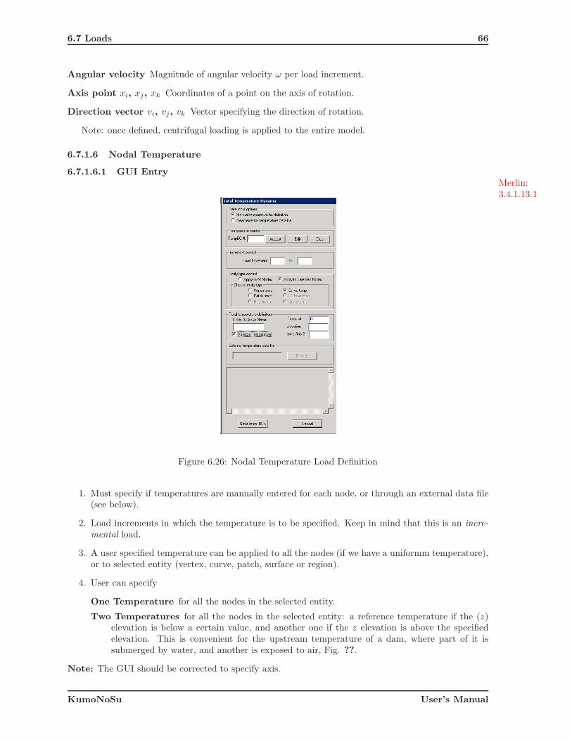
6.7 Loads 66

Angular velocity Magnitude of angular velocity ω per load increment.

Axis point xi, xj , xk Coordinates of a point on the axis of rotation.

Direction vector vi, vj, vk Vector specifying the direction of rotation.

Note: once defined, centrifugal loading is applied to the entire model.

6.7.1.6 Nodal Temperature

6.7.1.6.1 GUI EntryMerlin:3.4.1.13.1

Figure 6.26: Nodal Temperature Load Definition

1. Must specify if temperatures are manually entered for each node, or through an external data file(see below).

2. Load increments in which the temperature is to be specified. Keep in mind that this is an incre-

mental load.

3. A user specified temperature can be applied to all the nodes (if we have a uniformm temperature),or to selected entity (vertex, curve, patch, surface or region).

4. User can specify

One Temperature for all the nodes in the selected entity.

Two Temperatures for all the nodes in the selected entity: a reference temperature if the (z)elevation is below a certain value, and another one if the z elevation is above the specifiedelevation. This is convenient for the upstream temperature of a dam, where part of it issubmerged by water, and another is exposed to air, Fig. ??.

Note: The GUI should be corrected to specify axis.


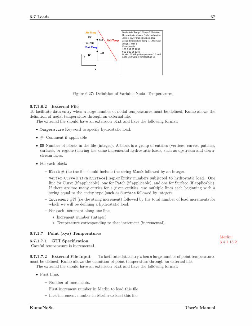
6.7 Loads 67

Air Temp

Pool Temp

Air2 Temp

x

y

512

125

Y=1250

12o

25o

Air Temp

Pool Temp

Air2 Temp

x

y

512

125

Y=1250

12o

25o

Node Axis Temp-1 Temp-2 Elevation If coordinate of node Node in direction Axis is lower that Elevation, then assign temperature Temp-1. Otherwise assign Temp-2 For example: 125 2 12 25 1250 512 2 12 25 1250 Node 125 will get temperature 12, and node 512 will get temperature 25

Figure 6.27: Definition of Variable Nodal Temperatures

6.7.1.6.2 External FileTo facilitate data entry when a large number of nodal temperatures must be defined, Kumo allows thedefinition of nodal temperature through an external file.

The external file should have an extension .dat and have the following format:

• Temperature Keyword to specify hydrostatic load.

• # Comment if applicable

• NB Number of blocks in the file (integer). A block is a group of entities (vertices, curves, patches,surfaces, or regions) having the same incremental hydrostatic loads, such as upstream and down-stream faces.

• For each block:

– Block # (i.e the file should include the string Block followed by an integer.

– Vertex|Curve|Patch|Surface|RegionEntity numbers subjected to hydrostatic load. Oneline for Curve (if applicable), one for Patch (if applicable), and one for Surface (if applicable).If there are too many entries for a given entities, use multiple lines each beginning with astring equal to the entity type (such as Surface followed by integers.

– Increment #N (i.e the string increment) followed by the total number of load increments forwhich we will be defining a hydrostatic load.

– For each increment along one line:

∗ Increment number (integer)

∗ Temperature corresponding to that increment (incremental).

6.7.1.7 Point (xyz) TemperaturesMerlin:3.4.1.13.26.7.1.7.1 GUI Specification

Careful temperature is incremental.

6.7.1.7.2 External File Input To facilitate data entry when a large number of point temperaturesmust be defined, Kumo allows the definition of point temperaturs through an external file.


• First Line:

– Number of increments.

– First increment number in Merlin to load this file

– Last increment number in Merlin to load this file.


6.7 Loads 68

Figure 6.28: Point Temperature Load Definition

– Number of point temperatures.

– Spatial dimension (2 or 3).

• For each point temperature, specify on one line:

– id number (integer starting with 1).

– x,y,[z] coordinates.

• For each increment, specify on one line

– id number of point

– Temperature of the point. Note temperatures are incremental, hence the first increment de-fines the base temperature, and the second increment specifies the temperature increase/decreasewith respect to the previous one. Hence for any increment n, the temperature is equal toT1 + Σi=n

i=2 Ti.

6.7.2 Total Load Definition

Total loads are those which once applied, remain constant in all subsequent load increments.

6.7.2.1 HydrostaticMerlin:3.4.1.7.16.7.2.1.1 GUI Entries

Hydrostatic load is defined by Fig. 6.29.


Entity type Type of loaded entity (curve in 2D, patch or surface in 3D).



6.7 Loads 69

Figure 6.29: Hydrostatic Load Definition

Entity # Number of the loaded entity.

Elevation/inc Fluid elevation change per load increment (∆h)

Fluid weight Fluid weight density (force/volume).

Direction of fluid height in global coordinates, X-dir, Y-dir, or Z-dir (3D only).

Note that in general, a first load number must be defined which brings the water elevation to the baseof the dam. Then, incremental water height (∆h) can be defined to raise the water at each increment.

6.7.2.1.2 External FileTo facilitate data entry when a large number of hydrostatic loads must be defined, Kumo allows thedefinition of hydrostatic load through an external file.


• Hydrostatic Keyword to specify hydrostatic load.


• NB Number of blocks in the file (integer). A block is a group of entities (curves, patches or surfaces)having the same incremental hydrostatic loads, such as upstream and downstream faces.

• For each block:


– Curve|Patch|Surface Entity numbers subjected to hydrostatic load. One line for Curve (ifapplicable), one for Patch (if applicable), and one for Surface (if applicable). If there are toomany entries for a given entities, use multiple lines each beginning with a string equal to theentity type (such as Surface followed by integers.

– Increment #N (i.e the string increment) followed by the total number of load increments forwhich we will be defining a hydrostatic load.


6.7 Loads 70

– For each increment, and along the same line:


∗ ∆ Elevation of the reservoir. Note that this is the incremental elevation and not the totalelevation. Hence in the first increment we (typically) bring the pool elevation to the baseelevation of the dam (hence the dam is not loaded), and in subsequent increments wesimply specify by how much we raise (+ve) or lower (-ve) the pool.

∗ γw Fluid weight density

∗ Axis orientation (2 If fluid is along y, 1 if along the x)

6.7.2.2 Mud/Silt

Mud and silt load is sightly different than hydrostatic load, as the lateral pressure is equal to thevertical pressure times the passive coefficient k. For an inclined curve (2D) or patch (3D), KumoNoSuwill automatically calculate the mud/silt pressure normal to the surface, given the vertical and lateralcomponents Fa and Fl.

It is defined, as follows, Fig. 6.30.:

Figure 6.30: Mud Silt Definition




Entity # Number of the loaded entity.

Elevation/inc Fluid elevation change per load increment (∆h).

Fluid weight Fluid weight density (force/volume).

Passive pressure coeff. Passive pressure coefficient for lateral pressure due to mud/silt (k coefficient).

Direction of fluid height in global coordinates, X-dir, Y-dir, or Z-dir (3D only).

As for hydrostatic load, a first load number must be defined which brings the mud elevation to the baseof the dam. Then, incremental mud height (∆h) can be defined to raise the mud at each increment.


6.7 Loads 71

Figure 6.31: Westergaards Added Mass Load Definition


6.7 Loads 72

6.7.2.3 WestergaardMerlin:3.4.1.7.33.4.1.7.3

Westerggard’s pseudo-hydrodynamic added masses are determined as follows, Fig. 6.31:



Load # Number of current load (for reference).

Entity # number of the loaded entity.

Axis # Axis defining reservoir depth: 1 = X, 2 = Y, 3 = Z (3D only).

Elevation/inc Elevation of the reservoir surface per load increment note that this is not the relativedepth of the reservoir, but rather the elevation of the surface).

Rel. depth Relative depth of the reservoir.

K constant : K constant for Westergaard equation (defined by Westergaard as 51.0 lb/ft3 or 8,011.4N/m3 for water).

Fluid weight Weight per unit volume of the fluid.

Fluid modulus Elastic modulus of the fluid (may be taken as 300 kips/in2 or 2.068 GPa for water).

Gravity g Acceleration of gravity.

Seismic period Period of the earthquake motion.

Accel coeff Lateral acceleration as a fraction of gravity.

Pressure type Positive (towards dam) or negative.

Note that if the earthquake excitation is not along the stream axis, than an orthogonal model of theadded mass must be specified, Fig. 6.32:

0 0

0 0

0 0 z

x

yM m

αα

α

= , x uɺɺ

, y vɺɺ, z wɺɺ

xα

yα

zα 0 0

0 0

0 0 z

x

yM m

αα

α

= , x uɺɺ

, y vɺɺ, z wɺɺ

xα

yα

zα

, x uɺɺ

, y vɺɺ, z wɺɺ

xα

yα

zα

Figure 6.32: Westergaards Orhtogonal Added Mass Load Definition

6.7.2.4 UpliftMerlin:3.4.1.7.46.7.2.4.1 GUI Definition

Two uplift models are implemented in KumoNoSu :

Full is when we have an uplift pressure, only along a crack, equal to the upstream hydrostatic pressure.There is no uplift pressure from the crack tip to the downstream face.

Ferc is identical to Full, however there is a linearly varying pressure from the crack tip to the tailwaterhydrostatic pressure, Fig. 6.33.


6.7 Loads 73

��

��

��

��

L Drains

��

��TW

CL

C

��

��

TW

C

Drains

��

��

TW

L

H3

CL Drains

��

��

TW

Drains

��

��

��

��

��

��

��

��

��

��

��

��

��

��

��

��

��

��

��

��

��

��

��

��

��

��

��

��

��

��

��

��

TWH4

HW

L

HW

H4=HW

HW

TWH4

TL

H4<TW H3=K*(HW-TW)+TW

H4>TW H3=K*(HW-H4)+H4

H3

X

TWH4

HW

TL

H4<TW H3=(HW-TW)(K*(L-X)/L+(T/X)*(1-K*(L-X)/L))+TW

H4>TW H3=(HW-TW)(K*(L-X)/L+(T/X)*(1-K*(L-X)/L))+H4

X

HW

HW

TW

TL

HW

X

T>X and Piezometer readings not available

c)

a) b)

d)

Figure 6.33: FERC Uplift Loads


6.7 Loads 74

Figure 6.34: Uplift Load Definition

KumoNoSu defines the uplift as follows, Fig. 6.34:


Uplift model type Full uplift or the FERC model.

Load # Number of the current load (for reference).

Crack Path # Number of the crack path subjected to uplift pressures.

Axis # Axis defining reservoir depth: 1 = X, 2 = Y, 3 = Z (3D only).

Elevation/inc Fluid elevation per load increment.

Fluid weight Weight per unit volume of the fluid.

Crack prop axis # Global axis which defines the direction of crack propagation (necessary for 3Duplift only).

Crack surfaces subjected to uplift : Both sides, lower surface only, or upper surface only.

If the FERC model is used, Fig.6.33, then additional data must be entered:

Distance from crack mouth to the drain This is an average distance.

Drain efficiency e (0 < e < 1) where 1. corresponds to full efficiency)

• Before it is intersected by the crack. If there is no drain, specify 0.

• After it has been intersected by the crack.

Drain elevation Vertical distance between the crack subjected to uplift and the drain

Tail water elevation (or water elevation at the end of the crack).

Total base length of the dam, i.e from upstream to downstream. Note this is not the projected length,but the actual length of the crack. For multiple (inclined) segments, the total “curvilinear” lengthmust be specified. If the base length is variable, then it would be more conservative to adopt themaximum length.


6.7 Loads 75

6.7.2.4.2 External FileTo facilitate data entry when a large number of uplift loads must be defined, Kumo allows the definitionof uplift load through an external file.


• Uplift Keyword to specify hydrostatic load.


• NB Number of blocks in the file (integer). A block is a group of cracks having the same uplift load.

• For each block:


– Crack followed by the cracks defining this particular block.

– Increment #N (i.e the string increment) followed by the total number of load increments forwhich we will be defining an uplift load.

– For each increment, and along the same line:


∗ Water elevation in global coordinate system. Note that this is an incremental uplift to bedefined with respect to the previous total uplift pressure. Hence the very first incrementshould bring the uplift pressure to the dam reference elevation.

∗ Unit weight of water, γW .

∗ Id of the global coordinate axis along which the uplift is applied (x =1, y=2, z=3).

∗ Directions of uplift forces. 0: both sides, -1: lower side, 1: upper side.

∗ Direction of crack (from upstream to downstream): a) 2D: User must simply definedirection of ±1 if along ±x, and ±2 if along ±y. b) or 3D: User must define a vectorvx, vy , vz from upstream to downstream direction.

∗ If FERC Model is specified, continue on the same line by inserting

· FERC

· Distance from crack mouth to the drain

· Drain efficiency e (0 < e < 1) where 1. corresponds to full efficiency) before it isintersected by the crack. If there is no drain, specify 0.

· Drain efficiency after it has been intersected by the crack

· Vertical distance between the crack subjected to uplift and the drain

· Tail water elevation (or water elevation at the end of the crack) measured with respectto the crack subjected to uplift. Note that this is NOT incremental, but the totalelevation.

· Total base length of the dam from upstream to downstream. In 2D:User must specifythe length. in 3D: If left as 0., then Merlin internally computes this length, if non-zero, then Merlin will consider this value as the length. Note that this is not theprojected length, but the actual “curvilinear” length of the crack.

6.7.2.5 Dynamic Uplift

to insert Merlin:3.4.1.7.6

6.7.3 Reset Nodal DisplacementsMerlin:3.1.2This enables the user to rest the nodal displacements (but not the stresses or the state variables) to zero

after a certain increment, Fig. 6.35.


6.7 Loads 76

Figure 6.35: Reset (zero) Displacments Definition

6.7.4 Heat Transfer/Seepage Loads

MUST BE COMPLETED, CHECK POWER POINT FILES

6.7.4.1 Temperature

Temperature nodal loads can be specified not only for thermal effects but also for any other physicalphenomena causing expansion (such as Alkali-Silica Reactions, in conjunction with a pseudo coefficientof thermal expansion defined in the material properties), Fig. 6.36.

Figure 6.36: Temperature Load Definition


Entity type Type of loaded entity (vertex or curve in 2D, all entity types in 3D). Note that:

• If every node in the FE mesh is to receive a temperature bc, select Apply to all nodes.

• If the selected entity type has minor entities associated to it (such as the end vertices fora curve), those minor entities may be included by selecting Apply to associated minorentities.


6.7 Loads 77

TempBC # Number of current bc (for reference).

Entity # Number of the entity receiving temperature bcs.

Temp/inc Temperature change (∆T ) per load increment.

6.7.4.2 Head

Head load is defined as follows, Fig. 6.37.

Figure 6.37: Head Load Definition


Entity type Type of loaded entity (vertex or curve).

Head # Number of current head(for reference).

Entity # Number of the entity receiving the head bcs.

Head/inc Head per load increment.

6.7.5 Dynamic Analysis

This option is intended to be used for the application of an acceleration history for a dynamic analysis.Since the history is applied at load increment 1 of the dynamic analysis, no load increments or intervalsmay be specified, Fig. 6.38. Mandatory information:

Acceleration history file Name of text file containing the nodal acceleration history. This file shouldcontain: ti, axi, ayi, azi.

.pst file data dump Increment interval at which to write analysis results to the .pst output file forviewing with Spider.


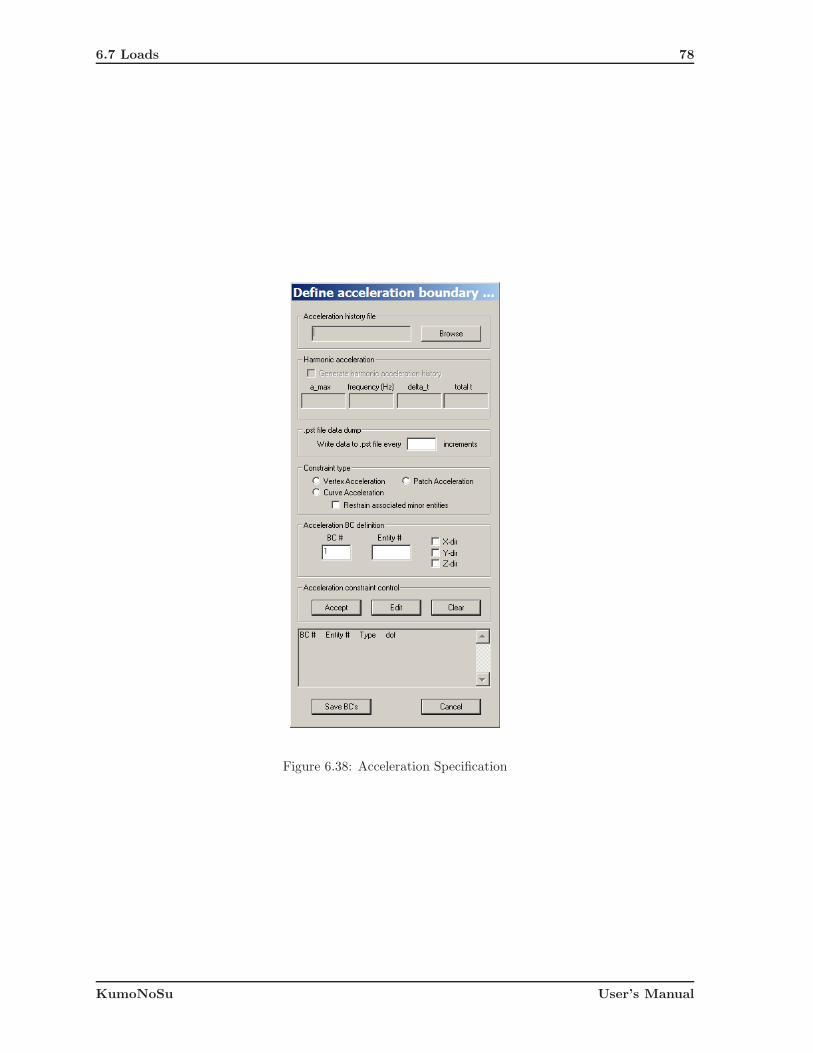
6.7 Loads 78

Figure 6.38: Acceleration Specification


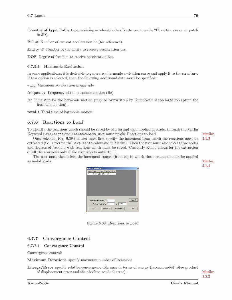
6.7 Loads 79

Constraint type Entity type receiving acceleration bcs (vertex or curve in 2D, vertex, curve, or patchin 3D).

BC # Number of current acceleration bc (for reference).

Entity # Number of the entity to receive acceleration bcs.

DOF Degree of freedom to receive acceleration bcs.

6.7.5.1 Harmonic Excitation

In some applications, it is desirable to generate a harmonic excitation curve and apply it to the structure.If this option is selected, then the following additional data must be specified:

amax Maximum acceleration magnitude.

frequency Frequency of the harmonic motion (Hz).

∆t Time step for the harmonic motion (may be overwritten by KumoNoSu if too large to capture theharmonic motion).

total t Total time of harmonic motion.

6.7.6 Reactions to Load

To identify the reactions which should be saved by Merlin and then applied as loads, through the MerlinKeyword SaveReacts and Reacts2Loads, user must invoke Reactions to load. Merlin:

3.1.3Once selected, Fig. 6.39 the user must first specify the increment from which the reactions must beextracted (i.e. generate the SaveReacts command in Merlin). Then the user must also select those nodesand degrees of freedom with reactions which must be saved. Currently Kumo allows for the extractionof all the reactions only if the user selects Auto-Fill.

The user must then select the increment ranges (from-to) to which those reactions must be appliedas nodal loads. Merlin:

3.1.4

Figure 6.39: Reactions to Load

6.7.7 Convergence Control

6.7.7.1 Convergence Control

Convergence control:

Maximum Iterations specify maximum number of iterations

Energy/Error specify relative convergence tolerance in terms of energy (recommended value productof displacement error and the absolute residual error). Merlin:

3.2.2


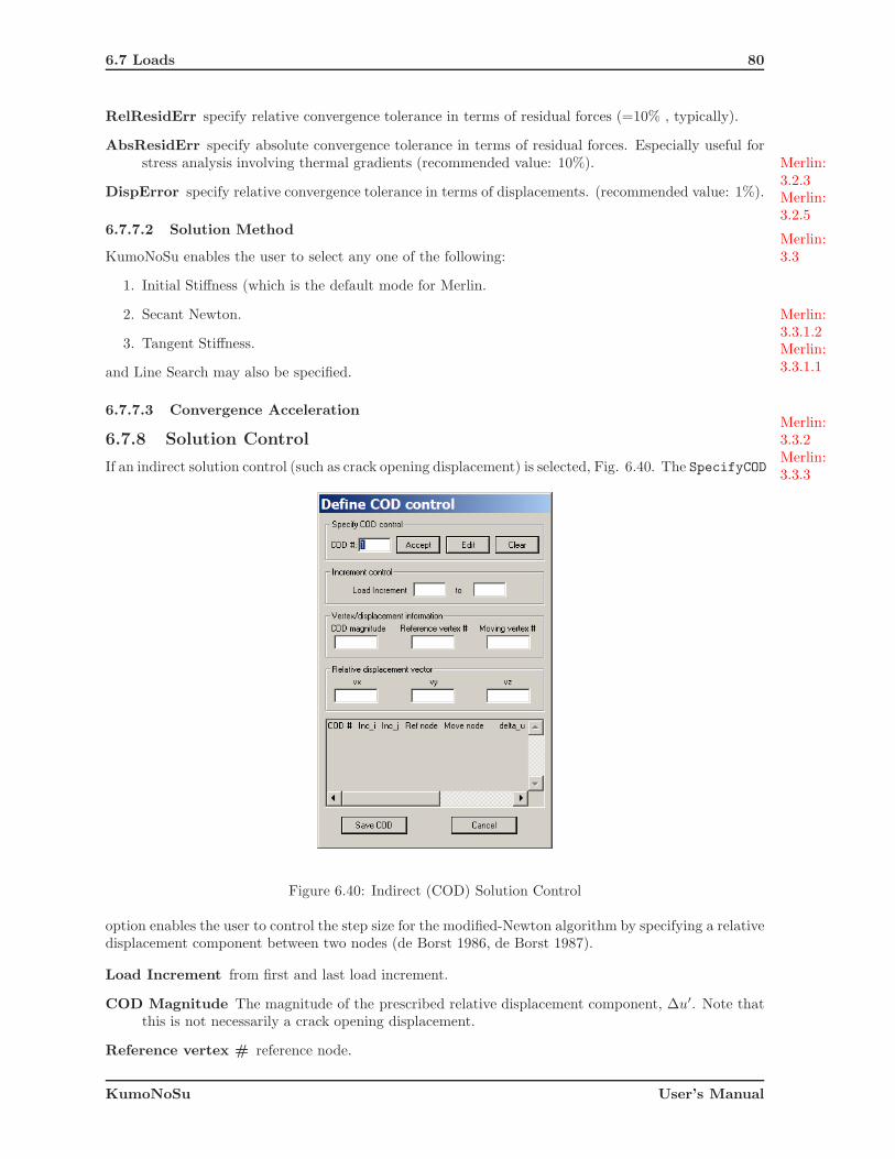
6.7 Loads 80

RelResidErr specify relative convergence tolerance in terms of residual forces (=10% , typically).

AbsResidErr specify absolute convergence tolerance in terms of residual forces. Especially useful forstress analysis involving thermal gradients (recommended value: 10%). Merlin:

3.2.3DispError specify relative convergence tolerance in terms of displacements. (recommended value: 1%). Merlin:

3.2.56.7.7.2 Solution Method

Merlin:3.3KumoNoSu enables the user to select any one of the following:

1. Initial Stiffness (which is the default mode for Merlin.

2. Secant Newton. Merlin:3.3.1.2

3. Tangent Stiffness. Merlin:3.3.1.1and Line Search may also be specified.

6.7.7.3 Convergence AccelerationMerlin:3.3.26.7.8 Solution ControlMerlin:3.3.3

If an indirect solution control (such as crack opening displacement) is selected, Fig. 6.40. The SpecifyCOD

Figure 6.40: Indirect (COD) Solution Control

option enables the user to control the step size for the modified-Newton algorithm by specifying a relativedisplacement component between two nodes (de Borst 1986, de Borst 1987).

Load Increment from first and last load increment.

COD Magnitude The magnitude of the prescribed relative displacement component, ∆u′. Note thatthis is not necessarily a crack opening displacement.

Reference vertex # reference node.


6.7 Loads 81

Moving vertex # second node.

vector components The three components vi of the vector v defining the direction of the relativedisplacement component.

The magnitude of the prescribed relative displacement component and the direction vector componentsare floating point numbers and the node numbers are integers. The relative displacements (in theglobal coordinate system) are defined by subtracting the displacements for the “moving” node from thedisplacements for the reference node. The direction vector v is not required to be a unit vector; theprogram utilizes it before computing the relative displacement component. For two-dimensional analysesthe third component vz of the vector v is not input; it is only input for three-dimensional analyses.

6.7.9 .pst File ControlMerlin:3.1.5This option, Fig. 6.41 enables the user to minimize the size of the .pst file (used both for restart, and

for the graphical postprocessor Spider. User can specify:

Case # Case number (for reference).

Load increment Specifies the range of increments inside which the .pst file is to be written at fixedinterval (different from the default of 1).

Write data to .pst file every Interval of .pst file update.

Figure 6.41: Suppress pst Output

6.7.10 Staged Construction/Excavation

Staged construction/excavation can be approximately simulated by the algorithms shown in Fig. 6.42and 6.43 respectively.

Though clearly an approximation, this approach was relatively simple to implement, and yieldsexcellent results.

1. With reference to Fig. 6.44, the user must begin by assigning the exact material properties for

Construction all the materials, or only the reference material id. Kumo will assign an initialscaled value of E corresponding to the user entered value to the other groups.

Excavation Assign the exact material properties to all the elements.

2. Specify the reference material group id (the one with the exact properties).

3. Specify the scaling factor for E corresponding to the “ghost” elements.

4. Specify the order for construction/excavation.

It should be noted that 2 increments are needed for each additional layer of excavation or construction.Hence if not enough increments have been specified, kumo will issue a warning message, Fig. 6.45.


6.7 Loads 82

Step 1: define material 1 real properties (E, ν, ρ)define “reduced” properties for all the others (E ≅ 0, ρ = 0)

apply gravity (Body Force List) only to material group 1 (all increments)Step 2: change material 2 properties (E, ν, ρ)Step 3 apply gravity (Body Force List) only to material groups 1 and 2 (all increments)Step 4: change material 3 properties (E, ν, ρ)Step 5: apply gravity (Body Force List) to material groups 1,2 and 3 (all increments)Step 6: change material 4 properties (E, ν, ρ)Step 7: apply gravity (Body Force List) to all materials (all increments)

Construction in 3 stages

Step 1 Step 2 Step 3 Step 4

LegendReduced propertiesChange propertiesApply gravity

Step 5 Step 6 Step 7

Figure 6.42: Algorithm for Staged Construction

Excavation in 3 stages

Step 1: define real properties (E, ν, ρ) for all materialsapply gravity (Body Force List) to all material groups (all increments)

Step 2: apply opposite gravity (Body Force List) to material groups 4 (all increments)Step 3: change material 4 properties (“reduced” properties E, ρ ≅ 0)



Step 1 Step 2 Step 3 Step 4

LegendReduced propertiesApply opposite gravityApply gravity

Step 5 Step 6 Step 7

Figure 6.43: Algorithm for Staged Excavation


6.8 Incremental Material Update 83

Figure 6.44: Graphical User Interface for Staged Construction/Excavation

Figure 6.45: Staged COnstruction/Excavation Warning if Insufficient number of Increments Specifiedn

6.8 Incremental Material Update

This option enables the user to modify material properties after the first increment. Hence, during aload increment, user can alter any of the existing material properties, Fig. 6.46.

Figure 6.46: Incremental material Update

This option is useful to alter the material properties from the static ones, to dynamic ones after arestart. This can also be used to simulate stage construction by adding the mass and increasing theYoung’s modulus incrementally.

6.9 Generate Free FieldMerlin-T:5.3.2Fig. 6.47 shows how to generate the free field meshes.


6.10 Run Free Field 84

Figure 6.47: Generate Free Field

The user has the following options:

1. Specify the left and right curves (2D) or left, right, front and back patches (3D) with respect towhich the free field mesh will be generated.

2. Specify type of dampers

(a) Interface (strongly recommended) continuous element dampers

(b) nodal dampers

3. Excitation data file (should be same as the one applied to the foundation).

4. Active degrees of freedom. If only x excitation is specified in the excitation data file, then checkthe x box, same with the others.

5. Force Inactive DOF to zero (recommended).

6. There are two options to transfer results of free field

Nodal Velocities/Displacements This option is discouraged though in 2D transfer of velocitieshas been shown to yield good results.

Forces (Recommended). Results of free field analysis can be transferred as nodal forces based on

(a) Stiffness (this will cause vertical forces)

(b) Damping

• Lysmer Damping (Strongly Recommended).

• Rayleigh damping (if forces based on stiffness are being transferred). In this case usermust specify the damping factor hd corresponding to the frequency f .

6.10 Run Free Field

This will simply run all the free field analysis, and then transfer the appropriate results to the merlininput data file of the main structure, Fig. 6.48.


6.11 Write .ctrl file 85

Figure 6.48: Complete Free Field Analysis Message

6.11 Write .ctrl file

A .ctrl file is needed to run the T3D2Merlin module. It should be noted that the Merlin input datafile will be assigned the same filename as the one of the .ctrl file.

6.12 Generate Merlin .inp file

With all preliminary steps completed, the user may generate the *.inp-file for Merlin’s analysis. The*.inp-file weds the geometric data (*.t3d-file) to the material properties and load data (*.ctrl-file). Fig.6.47... Note that if a parallel explicit analysis is to be performed, user should specify the number of

Figure 6.49: Generate Merlin Input File

processor, and an internal domain decomposition will be performed.


Chapter 7

Merlin Files

MerlinToolBox: Windows based driver for the following three programs.

KumoNoSu: Mesh Generator.

Merlin: Finite Element analysis program.

Spider: Graphical postprocessor

MATLAB: Based Drivers for Parameter Identification through Least Square Minimization

Figure 7.1: Merlin Toolbox

Extension Used by Generated byMerlin Specific Files

.inp Merlin input file KumoNoSu/T3D2Merlin

.out, .dyn Merlin output text files Merlin

.pst, .eig, .rtv Spider input file MerlinKumoNoSu Specific Files

.bd T3D input file KumoNoSu

.t3d T3D output file T3D

.ctrl T3D2Merlin input file KumoNoSuBeaver Specific Files

.dam Beaver Beaver

.bd KumoNoSu Beaver

.ctrl KumoNoSu Beaver

Table 7.1: File Types

87

Kumo

MERLIN

Spider

.bd .ctrl .t3d

.inp

.pst

.out

.eig.rtv

.eps

Ana

lysi

s

.EMF

.eps

Pre

proc

esso

r

Postprocessor

Kumo

MERLIN

Spider

.bd .ctrl .t3d

.inp

.pst

.out

.eig.rtv

.eps

Ana

lysi

s

.EMF

.eps

Pre

proc

esso

r

Postprocessor

Figure 7.2: Program Interactions


88

DEFINE BOUNDARY

(.bd file)

GENERATE MESH

(.t3d file)

DEFINE MATERIAL PARAMETERS AND LOAD CASES

(.ctrl file)

CREATE MERLIN INPUT FILE

(.inp file)

KumoNoSuKumoNoSu

RUN MERLIN ANALYSISMerlinMerlin

SpiderSpiderVIEW RESULTS;

DEFINE BOUNDARY

(.bd file)

DEFINE BOUNDARY

(.bd file)

GENERATE MESH

(.t3d file)

GENERATE MESH

(.t3d file)


(.ctrl file)


(.ctrl file)


(.inp file)


(.inp file)

KumoNoSuKumoNoSu

RUN MERLIN ANALYSISMerlinMerlin

SpiderSpiderVIEW RESULTS;


DEFINE BOUNDARY

(.bd file)

GENERATE MESH

(.t3d file)


(.ctrl file)

CREATE MERLIN INPUT FILE FOR DYNAMIC STEP 1 INPUT FILE

(.inp file)

KumoNoSuKumoNoSu

RUN MERLIN STATIC ANALYSIS

MerlinMerlin

SpiderSpiderVIEW RESULTS; (.pst; .rtv; .eig)

USING SAME .bd AND .t3d FILES, DEFINE A NEW .ctrl FILE TO

GENERATE THE DYNAMIC STEP 2 INPUT FILE (RESTART FILE)

RUN MERLIN DYNAMIC ANALYSIS WITH RESTART PROVIDED BY STATIC .pst FILE

MerlinMerlin

KumoNoSuKumoNoSu

DEFINE BOUNDARY

(.bd file)

DEFINE BOUNDARY

(.bd file)

GENERATE MESH

(.t3d file)

GENERATE MESH

(.t3d file)


(.ctrl file)


(.ctrl file)

CREATE MERLIN INPUT FILE FOR DYNAMIC STEP 1 INPUT FILE

(.inp file)

KumoNoSuKumoNoSu


MerlinMerlin


MerlinMerlin

SpiderSpiderVIEW RESULTS; (.pst; .rtv; .eig)

USING SAME .bd AND .t3d FILES, DEFINE A NEW .ctrl FILE TO

GENERATE THE DYNAMIC STEP 2 INPUT FILE (RESTART FILE)


MerlinMerlin


MerlinMerlin

KumoNoSuKumoNoSu



89

Entity Geometry TopologyRegion free -List of boundary surfaces, patches, and shells

-List of fixed vertices, curves, surfaces, patches, and shellsSurface Rational Bezier surface 4 bounding curves

-List of fixed vertices, curves, and surfaces-Parent region or surface-Regions on both sides

Patch Plane -List of boundary curves-List of fixed vertices and curves-Parent region-Regions on both sides

Shell Rational Bezier surface -List of boundary curves-List of fixed vertices and curves-Parent region-Regions on both sides

Curve Rational Bezier curve -2 bounding vertices-List of fixed vertices and curves-Parent region, surface, patch, shell, or curve-List of connected surfaces, patches, and shells

Vertex Point -Parent region, surface, patch, shell, or curve-Parent vertex-List of fixed vertices-List of connected curves

Table 7.2: Hierarchy of Model Represenatation


Appendix A

MESH GENERATION

A.1 Introduction

Finite element mesh generation is now an integral part of a finite element analysis. With the increasedcomputational capabilities, increasingly more complex structures are being analysed. Those structuresmust be discretized.

The task is one of developing a mathematical model (discretization or tessalation) of a continuummodel. This is not only necessary in finite elment analysis, but in computer graphics/rendering also. Incomputer graphics, we focus on the boundary representation, and assign colors and shades on the basisof light source and outward normal direction of the polygon.

Hence, in the most general case, meshing can be defined as the process of breaking up a physicaldomain into smaller sub-domains (elements) in order to facilitate the numerical solution of a partialdifferential equation. Surface domains may be subdivided into triangle or quadrilateral shapes, whilevolumes may be subdivided primarily into tetrahedra or hexahedra shapes. The shape and distributionof the elements is ideally defined by automatic meshing algorithms.

1. Point placement, followed by triangularization (discussed below).

2. Sub-domain removal. Elements are gradually removed from the domain, one ata time, until thewhole domain is decomposed int finite elements.

3. Recursive subdivision. The domain is broken into simpler parts until the individual parts are singleelements or simple regions, that can be meshed directly, for instance by the conformal mappingalgorithm.

4. Hierarchical decomposition. The basic principle of a quadtree (or hierarchical decomposition) isto cover a planar region of interest by a square, then recursively partition squares into smallersquares until each square contains a suitably uniform subset of the input.

A.2 Triangulation

The concept of Voronoi diagrams first appeared in works of Descartes as early as 1644. Descartes usedVoronoi-like diagrams to show the disposition of matter in the solar system and its environs.

The first man who studied the Voronoi diagram as a concept was a German mathematician G. L.Dirichlet. He studied the two- and three dimensional case and that is why this concept is also known asDirichlet tessellation. However it is much better known as a Voronoi diagram because another Germanmathematician M. G. Voronoi in 1908 studied the concept and defined it for a more general n-dimensionalcase.

Very soon after it was defined by Voronoi it was developed independently in other areas like me-teorology and crystalography. Thiessen developed it in meteorology in 1911 as an aid to computingmore accurate estimates of regional rainfall averages. In the field of crystalography German researchers

A.2 Triangulation 91

dominated and Niggli in 1927 introduced the term Wirkungsbereich (area of influence) as a reference toa Voronoi diagram.

During the years this concept kept being rediscovered over and over again in different fields of scienceand today it is extensively used in about 15 different fields of sciences. Some of them being mathematics,computer science, biology, cartography, physiology and many others.

Vc

1 2 3 4

5

6Voronoi

Delaunay

6 f

4 f

a b

c

V Va b

ρ

Figure A.1: Voronoi and Delaunay Tessellation

A.2.1 Voronoi Polygon

Given a finite set of poits in the plane, the idea is to assign to each point a region of influence in such away that the regions decompose the plane, (?). To describe a specific way to do that, let S be a subsetof R

2 (S ⊆ R2). We define the Voronoi region of p ∈ S as the set of points x ∈ R that are at least as

close to p as to any other points in S:

Vp ={

x ∈ R2 | ||x − p|| ≤‖ x − 1 ‖, ∀q ∈ S

}

(A.1)

Each point x ∈ R2 has at least one nearest point in S, so it lies in at least one Voronoi region. Two

Voronoi regions lie on opposite sides of the perpendicular bisector separating the two generating points.

A.2.2 Delaunay Triangulation

The dual of the Voronoi diagram is obtained by drawing straight Delaunay edges connecting pointsp, q ∈ S if and only if their Voronoi regions intersect along a common line segment. Thus in general,the Delaunay edges decompose the convex hull of S into triangular regions which are referred to asDelaunay triangles, (?).

Using Euler’s relation, it can be shown that a planar graph with n ≥ 3 vertices has at most 3n − 6edges and at most 2n− 4 faces. THe same bounds hold for the number of Delaunay edges and triangles.Each Voronoi vertex u = Va∩Vb∩Vc is the center of a circle with radius ρ =‖ u−a ‖=‖ u−b ‖=‖ u−c ‖.The circle is empty because it encloses no point of S.

Additional detailed information on Voronoi tesselation, (?) is an excellent reference.

A.2.3 MATLAB Code

rand(’state’,4);

x = rand(1,3);

y = rand(1,3);

TRI = delaunay(x,y);

subplot(1,2,1),...

trimesh(TRI,x,y,zeros(size(x))); view(2),...


A.3 Finite Element Mesh Generation 92

axis([0 1 0 1]); hold on;

plot(x,y,’o’);

set(gca,’box’,’on’);

[vx, vy] = voronoi(x,y,TRI);

subplot(1,2,2),...

plot(x,y,’r+’,vx,vy,’b-’),...

axis([0 1 0 1])

A.3 Finite Element Mesh Generation

A.3.1 Boundary Definition

In order to discretize the continuum into a finite element mesh, first key geometrical information of themust be specified hierarchically:

Vertices: with nodal coordinates, and approximate desired element size in the immediate vicinity (thusdescribing the mesh density).

Edges: which connect vertices. Those can be either linear segments, polylines, or curves.

Surfaces: composed of edges, defined counterclockwise.

Volumes: (3D only) composed of surfaces.

Associated with surfaces (2D0, or volumes (3D) are different material properties.Examples of the hierarchical boundary definition is shown in Fig. A.2 and A.3.

Figure A.2: Control Point for a 2D Mesh

A.3.2 Interior Node Generation

Once the boundary has been defined, we need to insert internal nodes at a spacing which respect therequired mesh density. There are numerous techniques to insert those internal nodes. We present oneapproach, FIg. A.4



Figure A.3: Control Point for a 3D Mesh

Generation of internal nodesin zone I within shrunk boundary

Region to be meshed Boundary discretization

Zonal decomposition with nodal density Boundary shrinking by ε

r

r

Disk

Zon

e I,

r1

Zon

e II

I, r

3

Zone II, r2

Figure A.4: A Two Dimensional Triangularization AlgorithmControl Point for a 3D Mesh



1. Decompose the region into a disjoint ensemble of subregions with equal mesh density.

2. Shrink the mesh to avoid elements near the boundary with very acute interior angles.

3. Starting with the first zone, circumscribe it by the smallest possible rectangle.

4. Superimpose a square rectangular grid over the circumscribing rectangle.

5. Use a random number generator to randomly generate one interior node in each square. A disk ofradius r centered at each node is used to test that no other surrounding nodes are enclosed in thedisk. If so, the node in question is regenerated.

An alternative approach consists in, (Cervenka, J. 1994)

1. Generating a triangularization compatible with the initial nodes.

2. Check lengths of the edges. If an edge does not satisfy the prescribed size r, a new node is insertedin the center of the edge. The prescribed size is interpolated between those of the vertices at eachend of the edge.

3. Repeat this operation until convergence.

4. Smoothen the elemnts to assure appropriate aspect ratios.

A.3.3 Final Triangularization

With boundary and interior nodes generated:

1. Determine the Voronoi polygons

2. Perform a Delaunay triangularization

3. Smoothen the mesh to ensure that all generated elements have a satisfactory aspect ratio.

It should be noted that recent algorithms, which can generate quadrilateral elements out of the Delaunaytriangularization have recently emerged.


Appendix B

Rational Bezier Curve

The rational Bezier curve is determined by a control polygon, as shown in Fig. B.1.

P0

P1P2

P3

Figure B.1: Example of Rational Bezier Curve and Its Control Polygon

The curve generally follows the shape of the control polygon, the first and the last points on thecurve are coincident with the first P0 and the last point P3 of the control polygon, and the the first andthe last segments of the control polygon coincide with the curve tangent at the starting and the endingpoints of the curve, respectively.

Mathematically, it can be represented by the following equation(?).

P (t) =

∑ni=0 wi Pi Bn

i (t)∑n

i=0 wi Bni (t)

, (B.1)

where P (t) is the point on the curve, Pi are Bezier control points, wi are weight of Bezier control points,Bn

i is Bernstein polynomials, t is an independent variable varying in range from 0 to 1, and n is thedegree of the polynomial defining the curve segment.

Bernstein polynomial function is defined as

Bni (t) =

(

n

i

)

ti(1 − t)n−i (B.2)

or recursively as

Bni (t) = (1 − t)Bn−1

i (t) + t Bn−1i−1 (t), (B.3)

where B00 = 1.

The curve order is equal to the number of polygon points n + 1. Therefore,a 4 point rational bezierpolygons results in a cubic curve whereas a 3 point one results in a quadratic curve.

In the mesh generator program, the point P0 and Pn correspond to the model vertices while theremaining points form the control polygon of the curve. In the particle model, the elliptical curve hasbeen used to define the inclusion. Therefore, to construct the rational Bezier curve the control points ofthe elliptical curve must be determined based on the degree of the polynomial of the elliptical curve.

B.1 Quadratic curve 96

B.1 Quadratic curve

In the T 3D (?) mesh generator used internally by Kumo(?), the quadratic curve of the elliptical arc isdefined as demonstrated in Fig. B.2.

w2w0

w1

α

sδ

φ

b

a

CP

Figure B.2: Elliptical Arc-Quadratic Curve

Equations for each the variables shown in Fig. B.2 can be summarized as follows.

δ = bsin2 α

2

cos α2

(B.4)

φ = a sinα

2(B.5)

s =sin α

2

cos α2

√

a2 cos2α

2+ b2 sin2 α

2(B.6)

w0 = w2 = 1 (B.7)

w1 = cosα

2(B.8)

α ∈ (0 : 2π)\ {π} (B.9)

where w0, w1, and w2 are weights of the bezier control points.The y coordinate of the control point CP is then determined by

yCP =φ

tan α2

+ δ (B.10)


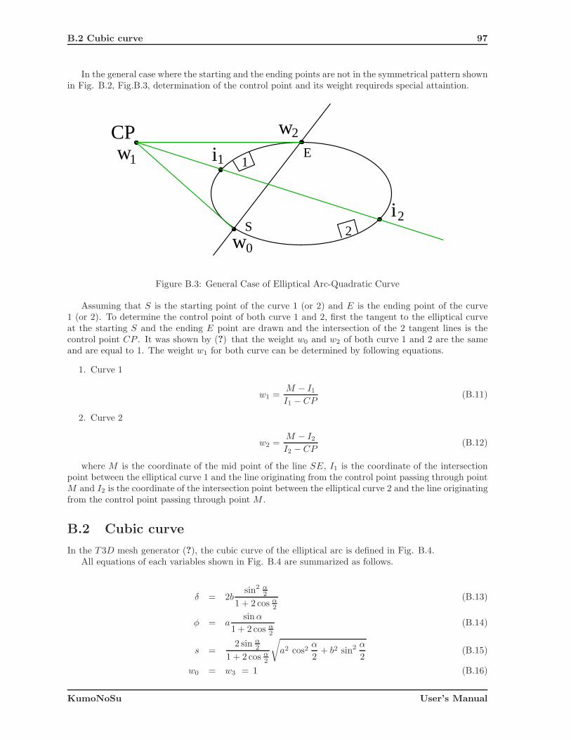
B.2 Cubic curve 97

In the general case where the starting and the ending points are not in the symmetrical pattern shownin Fig. B.2, Fig.B.3, determination of the control point and its weight requireds special attaintion.

w0

w1

w2CP1

i

i

22

1

S

E

Figure B.3: General Case of Elliptical Arc-Quadratic Curve

Assuming that S is the starting point of the curve 1 (or 2) and E is the ending point of the curve1 (or 2). To determine the control point of both curve 1 and 2, first the tangent to the elliptical curveat the starting S and the ending E point are drawn and the intersection of the 2 tangent lines is thecontrol point CP . It was shown by (?) that the weight w0 and w2 of both curve 1 and 2 are the sameand are equal to 1. The weight w1 for both curve can be determined by following equations.

1. Curve 1

w1 =M − I1

I1 − CP(B.11)

2. Curve 2

w2 =M − I2

I2 − CP(B.12)

where M is the coordinate of the mid point of the line SE, I1 is the coordinate of the intersectionpoint between the elliptical curve 1 and the line originating from the control point passing through pointM and I2 is the coordinate of the intersection point between the elliptical curve 2 and the line originatingfrom the control point passing through point M .

B.2 Cubic curve

In the T 3D mesh generator (?), the cubic curve of the elliptical arc is defined in Fig. B.4.All equations of each variables shown in Fig. B.4 are summarized as follows.

δ = 2bsin2 α

2

1 + 2 cos α2

(B.13)

φ = asin α

1 + 2 cos α2

(B.14)

s =2 sin α

2

1 + 2 cos α2

√

a2 cos2α

2+ b2 sin2 α

2(B.15)

w0 = w3 = 1 (B.16)


B.2 Cubic curve 98

w0

w1 w2

w3

CP1 CP2

α

δ

φ

b

a

s

Figure B.4: Elliptical Arc-Cubic Curve

w1 = w2 =1 + 2 cos α

2

3(B.17)

α ∈ (0 : 2π)\

{

4

3π

}

(B.18)

where w0, w1, w2 and w3 are weights of the Bezier control points.The control points CP1 and CP2 are the points which have the distance s from starting point SP

and the ending point EP in the direction of the tangent line to the curve at the starting and the endingpoints, respectively.

In the case where the starting and the ending points are not in the symmetrical pattern as shown inFig. B.5, and both points are opposite to each other as shown in Fig.B.5.

The value of the weights of the Bezier curve are still the same as shown in Eq. B.16 and B.17.However, the coordinates of both control points CP1 and CP2 can be computed as follows.

From Fig.B.5, suppose SP and EP are the starting and the ending points of curve 1.

1. Draw the tangent line to the elliptical curve at the SP and EP and determine the slope of thetangent s1.

2. Draw a line from the origin O, which a slope equal to s1. This line intersects with curve 1 at pointP .

3. Draw a tangent line to the elliptical curve 1 at point P (slope = s2) until it intersects the tangentline originating from the staring and the ending points at point A and B, respectively.

4. Determine the distance d.


B.2 Cubic curve 99

s1

s2

s2

s1

CP1

CP2

1P

O

EP

SP

d

2d

A

B

Figure B.5: Specific Case of Elliptical Arc-Cubic Curve

5. Control points CP1 and CP2 are then the points from the starting and the ending points withdistance 2d in the direction of its tangent, respectively.


Appendix C

Examples of Finite ElementBoundary Definition Output Filesfrom PARSIFAL Program

C.1 Matrix and Inclusion without Interface elements

1

2

4

5

6

15

16

3

1 2

34

5 615 16

Y

X

Figure C.1: Matrix and inclusion without interface elements

Fig.C.1 illustrates an elliptical inclusion (inside ellipse) surrounded by a matrix (box), with a perfectlyrigid interface (outside ellipse) between the matrix and inclusion. The boundary description for thisproblem is defined using (8) vertices, (8) curves, (3) patches, and (4) master/slave relations. Theresulting .bd file can be shown as follows.

C.1 Matrix and Inclusion without Interface elements 101

vertex 1 xyz -1.00000000e+000 -1.00000000e+000 0.00000000e+000

vertex 2 xyz 1.00000000e+000 -1.00000000e+000 0.00000000e+000

vertex 3 xyz 1.00000000e+000 1.00000000e+000 0.00000000e+000

vertex 4 xyz -1.00000000e+000 1.00000000e+000 0.00000000e+000

vertex 5 xyz -5.00000000e-001 0.00000000e+000 0.00000000e+000

vertex 6 xyz 5.00000000e-001 0.00000000e+000 0.00000000e+000

vertex 15 xyz -5.00000000e-001 0.00000000e+000 0.00000000e+000

vertex 16 xyz 5.00000000e-001 0.00000000e+000 0.00000000e+000

curve 1 order 2 vertex 1 2





polygon 1 xyz 5.00000000e-001 2.50000000e-001 0.00000000e+000

weight 3.333e-001

polygon 2 xyz -5.00000000e-001 2.50000000e-001 0.00000000e+000

weight 3.333e-001


polygon 1 xyz 5.00000000e-001 -2.50000000e-001 0.00000000e+000

weight 3.333e-001

polygon 2 xyz -5.00000000e-001 -2.50000000e-001 0.00000000e+000

weight 3.333e-001


polygon 1 xyz 5.00000000e-001 2.50000000e-001 0.00000000e+000

weight 3.333e-001

polygon 2 xyz -5.00000000e-001 2.50000000e-001 0.00000000e+000

weight 3.333e-001


polygon 1 xyz 5.00000000e-001 -2.50000000e-001 0.00000000e+000

weight 3.333e-001

polygon 2 xyz -5.00000000e-001 -2.50000000e-001 0.00000000e+000

weight 3.333e-001

patch 1 normal 0.0000e+000 0.0000e+000 1.0000e+000 boundary curve 5 -6

size 5.000e-002 property 1


size def hole

patch 3 normal 0.0000e+000 0.0000e+000 1.0000e+000 boundary curve 1 2 3 4

size 1.000e-001 property 2 subpatch 2

masterslave 1 vertex 5 15

masterslave 2 vertex 6 16

masterslave 3 curve 5 15

masterslave 4 curve 6 16

Note that vertices 5 and 15 share the same coordinates, as do vertices 6 and 16. Additionally, curves5/15 and 6/16 share identical properties. However, these curves combine to form separate patches, withcurves 5,6 forming patch 1 and curves 15,16 forming patch 2. Additionally, patch 2 is defined as a hole,since it is simply providing the connection between the inclusion (patch 1) and the matrix (patch 3).Patch 2 serves as a subpatch for patch 3.

In order to enforce the rigid connection between the matrix and the inclusion, master/slave relation-ships are defined for vertices 5/15 and 6/16, and for curves 5/15 and 6/16. These relations effectively


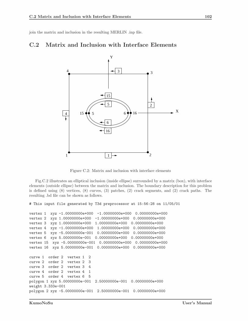
C.2 Matrix and Inclusion with Interface Elements 102

join the matrix and inclusion in the resulting MERLIN .inp file.

C.2 Matrix and Inclusion with Interface Elements

1

2

4

5

6

15

16

3

1 2

34

5 615 16

Y

X

Figure C.2: Matrix and inclusion with interface elements

Fig.C.2 illustrates an elliptical inclusion (inside ellipse) surrounded by a matrix (box), with interfaceelements (outside ellipse) between the matrix and inclusion. The boundary description for this problemis defined using (8) vertices, (8) curves, (3) patches, (2) crack segments, and (2) crack paths. Theresulting .bd file can be shown as follows.

# This input file generated by T3d preprocessor at 15:56:28 on 11/05/01

vertex 1 xyz -1.00000000e+000 -1.00000000e+000 0.00000000e+000

vertex 2 xyz 1.00000000e+000 -1.00000000e+000 0.00000000e+000

vertex 3 xyz 1.00000000e+000 1.00000000e+000 0.00000000e+000

vertex 4 xyz -1.00000000e+000 1.00000000e+000 0.00000000e+000

vertex 5 xyz -5.00000000e-001 0.00000000e+000 0.00000000e+000

vertex 6 xyz 5.00000000e-001 0.00000000e+000 0.00000000e+000

vertex 15 xyz -5.00000000e-001 0.00000000e+000 0.00000000e+000

vertex 16 xyz 5.00000000e-001 0.00000000e+000 0.00000000e+000






polygon 1 xyz 5.00000000e-001 2.50000000e-001 0.00000000e+000

weight 3.333e-001

polygon 2 xyz -5.00000000e-001 2.50000000e-001 0.00000000e+000


C.3 Matrix,Inclusion, and propagating Crack with Interface Elements 103

weight 3.333e-001


polygon 1 xyz 5.00000000e-001 -2.50000000e-001 0.00000000e+000

weight 3.333e-001

polygon 2 xyz -5.00000000e-001 -2.50000000e-001 0.00000000e+000

weight 3.333e-001


polygon 1 xyz 5.00000000e-001 2.50000000e-001 0.00000000e+000

weight 3.333e-001

polygon 2 xyz -5.00000000e-001 2.50000000e-001 0.00000000e+000

weight 3.333e-001


polygon 1 xyz 5.00000000e-001 -2.50000000e-001 0.00000000e+000

weight 3.333e-001

polygon 2 xyz -5.00000000e-001 -2.50000000e-001 0.00000000e+000

weight 3.333e-001




size def hole



crack NLFM

crack 1 structure curve 15 5


crack structure path 1 property 3


Note that vertices 5 and 15 share the same coordinates, as do vertices 6 and 16. Additionally, curves5/15 and 6/16 share identical properties. However, these curves combine to form separate patches, withcurves 5,6 forming patch 1 and curves 15,16 forming patch 2. Additionally, patch 2 is defined as a hole,since it is simply providing the connection between the inclusion (patch 1) and the matrix (patch 3).Patch 2 serves as a subpatch for patch 3.

In order to insert the interface elements between the matrix and the inclusion, structure crack seg-ments are defined between curves 5/15 and 6/16, and a two crack paths are defined using these twocrack segments. Since the crack type is defined as NLFM, interface elements will be inserted betweenthe matrix and inclusion in the MERLIN .inp file.

C.3 Matrix,Inclusion, and propagating Crack with Interface El-

ements

Fig.C.3 illustrates an elliptical inclusion (inside ellipse) surrounded by a matrix (box), with interfaceelements (outside ellipse) between the matrix and inclusion. Additionally, a crack extends from theright side of the inclusion (triangle). This crack, while represented by a triangle with a finite crackmouth opening in the above picture, is considered to have a zero thickness in the .bd file. The boundarydescription for this problem is defined using (10) vertices, (10) curves, (3) patches, (3) crack segments,and (2) crack paths. The resulting .bd file can be shown as follows.

# This input file generated by T3d preprocessor at 12:47:58 on 11/06/01

vertex 1 xyz -1.00000000e+000 -1.00000000e+000 0.00000000e+000


C.3 Matrix,Inclusion, and propagating Crack with Interface Elements 104

1

2

4

5

6

15

16

3

1 2

34

5 615

Y

X16

17

2020

21

Figure C.3: Matrix, inclusion, and propagating crack with interface elements

vertex 2 xyz 1.00000000e+000 -1.00000000e+000 0.00000000e+000

vertex 3 xyz 1.00000000e+000 1.00000000e+000 0.00000000e+000

vertex 4 xyz -1.00000000e+000 1.00000000e+000 0.00000000e+000

vertex 5 xyz -5.00000000e-001 0.00000000e+000 0.00000000e+000

vertex 6 xyz 5.00000000e-001 0.00000000e+000 0.00000000e+000

vertex 15 xyz -5.00000000e-001 0.00000000e+000 0.00000000e+000

vertex 16 xyz 5.00000000e-001 0.00000000e+000 0.00000000e+000

vertex 17 xyz 5.00000000e-001 0.00000000e+000 0.00000000e+000

coincide vertex 16

vertex 20 xyz 7.50000000e-001 0.00000000e+000 0.00000000e+000






polygon 1 xyz 5.00000000e-001 2.50000000e-001 0.00000000e+000

weight 3.333e-001

polygon 2 xyz -5.00000000e-001 2.50000000e-001 0.00000000e+000

weight 3.333e-001


polygon 1 xyz 5.00000000e-001 -2.50000000e-001 0.00000000e+000

weight 3.333e-001

polygon 2 xyz -5.00000000e-001 -2.50000000e-001 0.00000000e+000

weight 3.333e-001


polygon 1 xyz 5.00000000e-001 2.50000000e-001 0.00000000e+000

weight 3.333e-001


C.4 Matrix, Inclusion, and Two Propagating Cracks with Interface Elements 105

polygon 2 xyz -5.00000000e-001 2.50000000e-001 0.00000000e+000

weight 3.333e-001


polygon 1 xyz 5.00000000e-001 -2.50000000e-001 0.00000000e+000

weight 3.333e-001

polygon 2 xyz -5.00000000e-001 -2.50000000e-001 0.00000000e+000

weight 3.333e-001

curve 20 vertex 20 16

curve 21 vertex 20 17 coincide curve 20



patch 2 normal 0.0000e+000 0.0000e+000 1.0000e+000 boundary

curve 20 15 -16 -21 size def hole



crack NLFM

crack 1 structure curve 21 20 front2d 20



crack structure path 1 mat 3

crack structure path 2 3 mat 3

Note that vertices 5 and 15 share the same coordinates, as do vertices 6, 16, and 17. Vertices 16and 17, which form the mouth of the crack, are labeled as coincident. The crack propagating from theinclusion is formed using curves 20 and 21 (coincident), with vertex 20 serving as the crack front. Curves5/15 and 6/16 also share identical properties. However, these curves combine to form separate patches,with curves 5,6 forming patch 1 and curves 15,16 (with curves 20 and 21) forming patch 2. Additionally,patch 2 is defined as a hole, since it is providing the interface connection between the inclusion (patch1) and the matrix (patch 3). Patch 2 serves as a subpatch for patch 3.

Two separate crack paths are considered. The first is the crack propagating from the inclusion. Thiscrack path is defined by a single crack segment formed by curves 20 and 21, with the crack front atvertex 20. The second crack path surrounds the inclusion, and is formed by two crack segments (curves5/15 and 6/16).

C.4 Matrix, Inclusion, and Two Propagating Cracks with In-

terface Elements

Fig.C.4 illustrates an elliptical inclusion (inside ellipse) surrounded by a matrix (box), with interfaceelements (outside ellipse) between the matrix and inclusion. Additionally, cracks extends from the rightand left sides of the inclusion (triangle). This crack, while represented by a triangle with a finite crackmouth opening in the above picture, is considered to have a zero thickness in the .bd file. The boundarydescription for this problem is defined using (12) vertices, (12) curves, (3) patches, (4) crack segments,and (4) crack paths. The resulting .bd file can be shown as follows.

# This input file generated by Kumonosu at 11:48:44 on 11/07/01

vertex 1 xyz -1.00000000e+000 -1.00000000e+000 0.00000000e+000

vertex 2 xyz 1.00000000e+000 -1.00000000e+000 0.00000000e+000

vertex 3 xyz 1.00000000e+000 1.00000000e+000 0.00000000e+000

vertex 4 xyz -1.00000000e+000 1.00000000e+000 0.00000000e+000

vertex 5 xyz -5.00000000e-001 0.00000000e+000 0.00000000e+000

vertex 6 xyz 5.00000000e-001 0.00000000e+000 0.00000000e+000


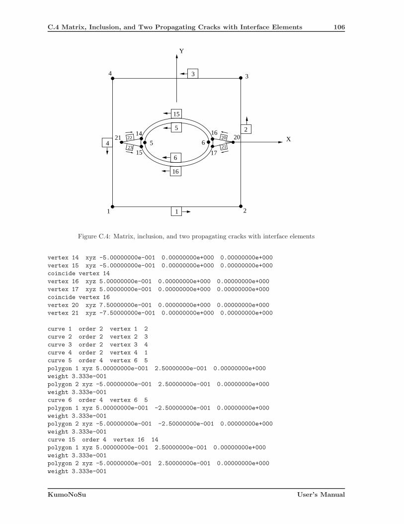
C.4 Matrix, Inclusion, and Two Propagating Cracks with Interface Elements 106

1

2

4

5

6

15

16

3

21

20

1 2

34

5 6

Y

X16

17

202114

15

22

23

Figure C.4: Matrix, inclusion, and two propagating cracks with interface elements

vertex 14 xyz -5.00000000e-001 0.00000000e+000 0.00000000e+000

vertex 15 xyz -5.00000000e-001 0.00000000e+000 0.00000000e+000

coincide vertex 14

vertex 16 xyz 5.00000000e-001 0.00000000e+000 0.00000000e+000

vertex 17 xyz 5.00000000e-001 0.00000000e+000 0.00000000e+000

coincide vertex 16

vertex 20 xyz 7.50000000e-001 0.00000000e+000 0.00000000e+000

vertex 21 xyz -7.50000000e-001 0.00000000e+000 0.00000000e+000






polygon 1 xyz 5.00000000e-001 2.50000000e-001 0.00000000e+000

weight 3.333e-001

polygon 2 xyz -5.00000000e-001 2.50000000e-001 0.00000000e+000

weight 3.333e-001


polygon 1 xyz 5.00000000e-001 -2.50000000e-001 0.00000000e+000

weight 3.333e-001

polygon 2 xyz -5.00000000e-001 -2.50000000e-001 0.00000000e+000

weight 3.333e-001


polygon 1 xyz 5.00000000e-001 2.50000000e-001 0.00000000e+000

weight 3.333e-001

polygon 2 xyz -5.00000000e-001 2.50000000e-001 0.00000000e+000

weight 3.333e-001


C.5 Matrix and Interior Crack with Interface Elements 107


polygon 1 xyz 5.00000000e-001 -2.50000000e-001 0.00000000e+000

weight 3.333e-001

polygon 2 xyz -5.00000000e-001 -2.50000000e-001 0.00000000e+000

weight 3.333e-001







patch 2 normal 0.0000e+000 0.0000e+000 1.0000e+000 boundary curve

20 15 -22 23 -16 -21 size def hole



crack NLFM









Unlike the example with a single propagating crack, in which the interface around the inclusion wastreated as a single crack path, this geometry requires that (4) crack paths are defined: one for the leftpropagating crack, one for the right propagating crack, and two paths around the inclusion (top andbottom). The rest of the boundary description is similar to that of the single crack example. There are(3) total patches: one for the inclusion, a second composed of the inclusion and the two cracks (definedas a hole), and a third which is composed of the matrix.

C.5 Matrix and Interior Crack with Interface Elements

Fig. C.5 illustrates an interior crack (red lines) surrounded by a matrix (yellow box). The boundarydescription for this problem is defined using (8) vertices, (8) curves, (1) patch, (2) crack segments, and(2) crack paths. The resulting .bd file is on the next page.

# This input file generated by Kumonosu at 14:21:05 on 11/29/01

vertex 1 xyz -1.00000000e+000 -1.00000000e+000 0.00000000e+000

vertex 2 xyz 1.00000000e+000 -1.00000000e+000 0.00000000e+000

vertex 3 xyz 1.00000000e+000 1.00000000e+000 0.00000000e+000

vertex 4 xyz -1.00000000e+000 1.00000000e+000 0.00000000e+000

vertex 5 xyz -5.00000000e-001 0.00000000e+000 0.00000000e+000

vertex 6 xyz 5.00000000e-001 0.00000000e+000 0.00000000e+000

vertex 7 xyz 0.00000000e+000 0.00000000e+000 0.00000000e+000

vertex 8 xyz 0.00000000e+000 0.00000000e+000 0.00000000e+000 coincide vertex 7




C.5 Matrix and Interior Crack with Interface Elements 108

1 2

3 4

5 6 X

Y

8

1

2

3

4

8

5 7

6 7

Figure C.5: Matrix, Crack inclusion with interface elements


C.6 Sphere 109




curve 6 order 2 vertex 5 7 coincide curve 5


curve 8 order 2 vertex 6 7 coincide curve 7

patch 1 normal 0.00000000e+000 0.00000000e+000 1.00000000e+000 boundary curve 1 2 3 4 \

boundary curve -5 6 -8 7 size 1.000e-001 property 1

crack NLFM





vertex 5000 xyz -5.00000000e-001 0.00000000e+000 0.00000000e+000 coincide vertex 5 slave node

vertex 5001 xyz 0.00000000e+000 0.00000000e+000 0.00000000e+000 coincide vertex 8 slave node

vertex 5002 xyz -5.00000000e-001 0.00000000e+000 0.00000000e+000 coincide vertex 5 slave node


vertex 5004 xyz 5.00000000e-001 0.00000000e+000 0.00000000e+000 coincide vertex 6 slave node


vertex 5006 xyz 5.00000000e-001 0.00000000e+000 0.00000000e+000 coincide vertex 6 slave node


curve 5000 vertex 5000 5001 order 2 coincide curve 5 slave element




Notice that the single interior crack is actually composed of two cracks. Curves 5/6 form one side of thecrack, while curves 7/8 form the other side. Vertices 5 and 6 serve as the crack fronts, and vertices 7and 8 (coinciding vertices) form the middle of the crack. An interior crack must have these coincidingvertices at its center. This boundary description contains only one patch, but this patch contains twodefinitions of boundary curves. The first set of boundary curves defines the edges of the matrix, whilethe second set of boundary curves defines the crack.

C.6 Sphere

##########

# sphere #

##########

# Comments from Daniel

# I would recommend you to use two surfaces, each for one hemisphere,

# and each one obtained by rotating cubic circular 180 degree arc

# by angle of 180 degree using cubic expansion in the direction of revolution.

# Here is the example of a sphere centered at origin with radius equal to one:

# t3d -d 0.1

vertex 1 xyz 1 0 0

vertex 2 xyz -1 0 0

curve 1 vertex 1 2 order 4


C.6 Sphere 110

polygon 1 xyz 1 2 0 weight 0.3333333333333

polygon 2 xyz -1 2 0 weight 0.3333333333333


polygon 1 xyz 1 -2 0 weight 0.3333333333333

polygon 2 xyz -1 -2 0 weight 0.3333333333333

# collapsed curve defined as ordinary 180 deg circular arc


polygon 1 poly 0 weight 0.3333333333333


# collapsed curve defined as ordinary 180 deg circular arc




surface 1 curve 1 3 2 4

# polygon of a 180 deg circular arc from polygon point 1 of curve 1

# to polygon point 1 of curve 2 in plane yz+

# weights of this new polygon are obtained by multiplication of weights

# corresponding to 180 deg circular arc by the weight of appropriate

# polygon point on revoluted curve (1/3 * 1/3)

polygon 1 1 xyz 1 2 4 weight 0.111111111111

polygon 2 1 xyz -1 2 4 weight 0.111111111111


# to polygon point 2 of curve 2 in plane yz+

polygon 1 2 xyz 1 -2 4 weight 0.111111111111

polygon 2 2 xyz -1 -2 4 weight 0.111111111111

# ordering of curves is different from surface 1 in order to get the

# normal pointing out of the sphere (but it is not necessary to ensure that)

surface 2 curve 2 4 1 3


# to polygon point 2 of curve 1 in plane yz-

polygon 1 1 xyz -1 -2 -4 weight 0.111111111111

polygon 2 1 xyz 1 -2 -4 weight 0.111111111111


# to polygon point 1 of curve 1 in plane yz-

polygon 1 2 xyz -1 2 -4 weight 0.111111111111

polygon 2 2 xyz 1 2 -4 weight 0.111111111111


kumonosu - university of colorado boulder

Documents