la interaccion es significativa y también los factores ... · a) analysis of variance for...
TRANSCRIPT

a) Analysis of Variance for Light output, using Adjusted SS for Tests Source DF Seq SS Adj SS Adj MS F P Glass type 2 150865 150865 75432 206.37 0.000 Temperature 2 1970335 1970335 985167 2695.26 0.000 Glass type*Temperature 4 290552 290552 72638 198.73 0.000 Error 18 6579 6579 366 Total 26 2418330 S = 19.1185 R-Sq = 99.73% R-Sq(adj) = 99.61%
La interaccion es significativa y también los factores individuales
b)No es posible hacer modelo debido a que el tipo de vidrio es una variable categorica
c)
40200-20-40
99
90
50
10
1
Residual
Pe
rce
nt
150012501000750500
40
20
0
-20
-40
Fitted Value
Re
sid
ua
l
403020100-10-20-30
12
9
6
3
0
Residual
Fre
qu
en
cy
2624222018161412108642
40
20
0
-20
-40
Observation Order
Re
sid
ua
l
Normal Probability Plot Versus Fits
Histogram Versus Order
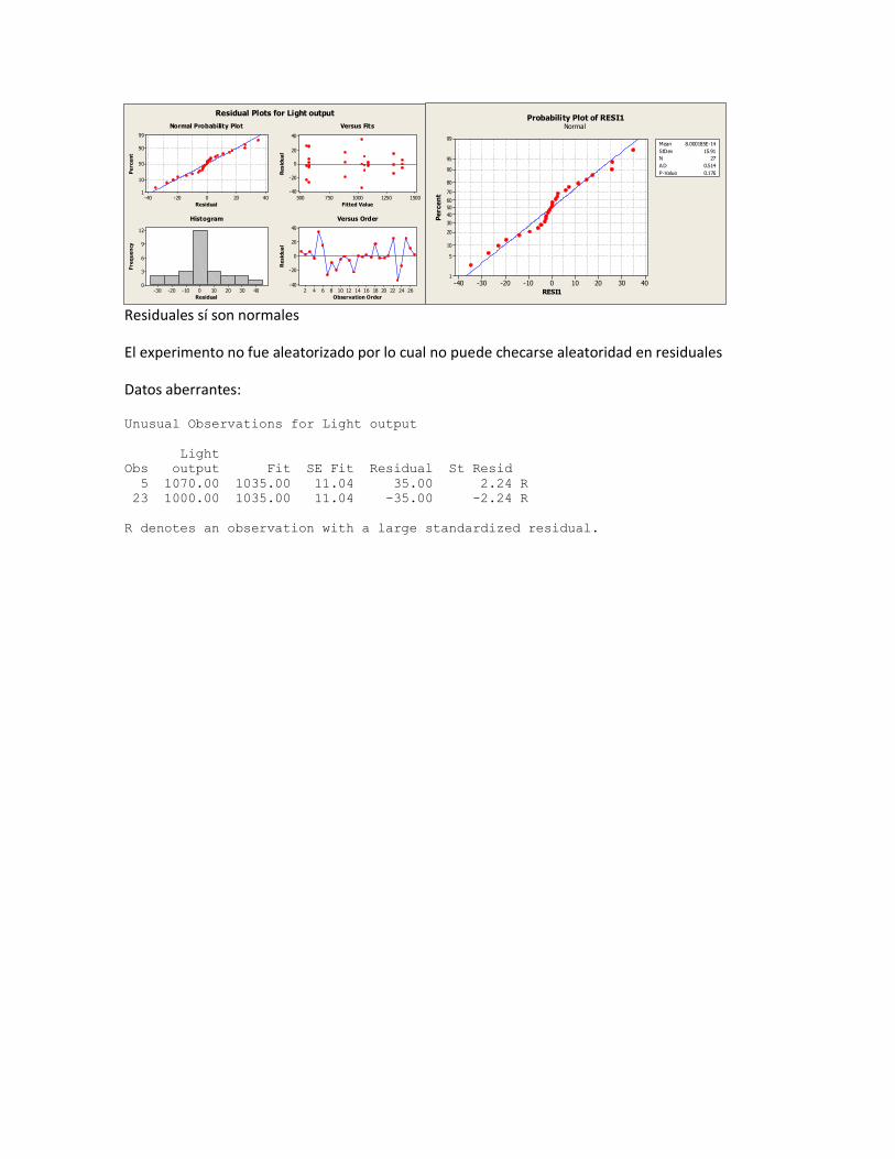
Residual Plots for Light output
403020100-10-20-30-40
99
95
90
80
70
60
50
40
30
20
10
5
1
RESI1
Pe
rce
nt
Mean 8.000185E-14
StDev 15.91
N 27
AD 0.514
P-Value 0.176
Probability Plot of RESI1Normal
Residuales sí son normales
El experimento no fue aleatorizado por lo cual no puede checarse aleatoridad en residuales
Datos aberrantes:
Unusual Observations for Light output Light Obs output Fit SE Fit Residual St Resid 5 1070.00 1035.00 11.04 35.00 2.24 R 23 1000.00 1035.00 11.04 -35.00 -2.24 R R denotes an observation with a large standardized residual.

a) Analysis of Variance for strength, using Adjusted SS for Tests Source DF Seq SS Adj SS Adj MS F P % hardwood 2 7.7639 7.7639 3.8819 10.62 0.001 cooking time 1 20.2500 20.2500 20.2500 55.40 0.000 pressure 2 19.3739 19.3739 9.6869 26.50 0.000 % hardwood*cooking time 2 2.0817 2.0817 1.0408 2.85 0.084 % hardwood*pressure 4 6.0911 6.0911 1.5228 4.17 0.015 cooking time*pressure 2 2.1950 2.1950 1.0975 3.00 0.075 % hardwood*cooking time*pressure 4 1.9733 1.9733 0.4933 1.35 0.290

Error 18 6.5800 6.5800 0.3656 Total 35 66.3089 S = 0.604612 R-Sq = 90.08% R-Sq(adj) = 80.70%
Factores individuales son significativos y la interacción % hardwood*pressure
b)
1.00.50.0-0.5-1.0
99
90
50
10
1
Residual
Pe
rce
nt
200198196
1.0
0.5
0.0
-0.5
-1.0
Fitted Value
Re
sid
ua
l
0.80.40.0-0.4-0.8
12
9
6
3
0
Residual
Fre
qu
en
cy
35302520151051
1.0
0.5
0.0
-0.5
-1.0
Observation Order
Re
sid
ual
Normal Probability Plot Versus Fits
Histogram Versus Order
Residual Plots for strength
1.00.50.0-0.5-1.0
99
95
90
80
70
60
50
40
30
20
10
5
1
RESI1
Pe
rce
nt
Mean 1.184238E-14
StDev 0.4336
N 36
AD 1.090
P-Value 0.006
Probability Plot of RESI1Normal
Residuales no son normales
No hay datos aberrantes
Aleatorización no puede checarse ya que el experimento no fue aleatorizado

c)
842
199.0
198.5
198.0
197.5
43
650500400
199.0
198.5
198.0
197.5
% hardwoodM
ea
ncooking time
pressure
Main Effects Plot for strengthData Means
43 650500400
200
198
196200
198
196
% hardwood
cooking time
pressure
2
4
8
% hardwood
3
4
time
cooking
Interaction Plot for strengthData Means
Condiciones optimas: %hardwood:2, cooking time 4, pressure 650

a) Analysis of Variance for warping, using Adjusted SS for Tests Source DF Seq SS Adj SS Adj MS F P Temperature 3 156.094 156.094 52.031 7.67 0.002 Cooper content 3 698.344 698.344 232.781 34.33 0.000 Temperature*Cooper content 9 113.781 113.781 12.642 1.86 0.133 Error 16 108.500 108.500 6.781 Total 31 1076.719
Ambos factores afectan

b)
5.02.50.0-2.5-5.0
99
90
50
10
1
Residual
Pe
rce
nt
3025201510
4
2
0
-2
-4
Fitted Value
Re
sid
ua
l43210-1-2-3
8
6
4
2
0
Residual
Fre
qu
en
cy
3230282624222018161412108642
4
2
0
-2
-4
Observation Order
Re
sid
ua
l
Normal Probability Plot Versus Fits
Histogram Versus Order
Residual Plots for warping
543210-1-2-3-4
99
95
90
80
70
60
50
40
30
20
10
5
1
RESI1
Pe
rce
nt
Mean 2.220446E-16
StDev 1.871
N 32
AD 0.666
P-Value 0.074
Probability Plot of RESI1Normal
La prueba de normalidad la pasa muy justa, no se ven bien distribuidos losresiduales
c) 1251007550
30.0
27.5
25.0
22.5
20.0
17.5
15.0
100806040
Temperature
Me
an
Cooper content
Main Effects Plot for warpingData Means
La temperatura no se comporta linealmente

100806040
30
25
20
15
10
Cooper content
Me
an
50
75
100
125
Temperature
Interaction Plot for warpingData Means
Dado que la interacción no es significativa, no afecta dónde debe estar la temperatura para elegir
el contenido de cobre bajo.
d) Misma respuesta que c)

a)
The regression equation is Y (strength) = 144 + 1.88 X (% hardwood)
b)
Analysis of Variance Source DF SS MS F P Regression 1 1262.1 1262.1 260.00 0.000 Residual Error 8 38.8 4.9 Total 9 1300.9
La regresión es significativa

a)
The regression equation is y = 351 - 1.27 x1 - 0.154 x2
b)
S = 25.4979 R-Sq = 86.2% R-Sq(adj) = 77.0% Analysis of Variance Source DF SS MS F P Regression 2 12161.6 6080.8 9.35 0.051 Residual Error 3 1950.4 650.1 Total 5 14112.0
Regresión significativa
c)
Predictor Coef SE Coef T P Constant 350.99 74.75 4.70 0.018 x1 -1.272 1.169 -1.09 0.356 x2 -0.15390 0.08953 -1.72 0.184
Ninguna de las pendientes es estadísticamente igual a cero porque los p-valores son mayores a
0.05

The regression equation is y = 24.4 - 38.0 x1 + 0.7 x2 + 35.0 x1^2 + 11.1 x2^2 - 9.99 x1x2 Predictor Coef SE Coef T P Constant 24.41 26.59 0.92 0.394 x1 -38.03 40.45 -0.94 0.383 x2 0.72 11.69 0.06 0.953 x1^2 34.98 21.56 1.62 0.156 x2^2 11.066 3.158 3.50 0.013 x1x2 -9.986 8.742 -1.14 0.297 S = 6.04244 R-Sq = 99.4% R-Sq(adj) = 98.9% Analysis of Variance Source DF SS MS F P Regression 5 35092.6 7018.5 192.23 0.000 Residual Error 6 219.1 36.5 Total 11 35311.7

Es una buena regresión porque R2 es grande, pero podemos notar que la regresión está dominada
por x2 solamente, los demás regresores no son significativos.
Analysis of Variance for Num orders (coded units) Source DF Seq SS Adj SS Adj MS F P Main Effects 3 50.500 50.500 16.833 5.61 0.023 A 1 12.250 12.250 12.250 4.08 0.078 B 1 2.250 2.250 2.250 0.75 0.412 C 1 36.000 36.000 36.000 12.00 0.009 2-Way Interactions 3 191.250 191.250 63.750 21.25 0.000 A*B 1 42.250 42.250 42.250 14.08 0.006 A*C 1 100.000 100.000 100.000 33.33 0.000 B*C 1 49.000 49.000 49.000 16.33 0.004 3-Way Interactions 1 4.000 4.000 4.000 1.33 0.282 A*B*C 1 4.000 4.000 4.000 1.33 0.282 Residual Error 8 24.000 24.000 3.000 Pure Error 8 24.000 24.000 3.000 Total 15 269.750
Significativos: C, A*B, A*C, B*C

3.01.50.0-1.5-3.0
99
90
50
10
1
Residual
Pe
rce
nt
5451484542
2
1
0
-1
-2
Fitted Value
Re
sid
ua
l
210-1-2
3
2
1
0
Residual
Fre
qu
en
cy
16151413121110987654321
2
1
0
-1
-2
Observation Order
Re
sid
ua
l
Normal Probability Plot Versus Fits
Histogram Versus Order
Residual Plots for Num orders
3210-1-2-3
99
95
90
80
70
60
50
40
30
20
10
5
1
RESI1
Pe
rce
nt
Mean 0
StDev 1.265
N 16
AD 0.504
P-Value 0.174
Probability Plot of RESI1Normal
Residuales normales, pero falta resolución en el instrumento de medición
Residual vs fits ligeramente forma de embudo
c)
1-1
49
48
47
46
1-1
1-1
49
48
47
46
A
Me
an
B
C
Main Effects Plot for Num ordersData Means

1
-1
1
-1
1-1
C
B
A
55.0
46.547.5
47.5
42.5
43.052.0
47.0
Cube Plot (data means) for Num orders
Se recomienda trabajar en A alto, B alto, C alto


a)
Estimated Effects and Coefficients for crack length (coded units) Term Effect Coef SE Coef T P Constant 11.988 0.05036 238.04 0.000 A 3.019 1.509 0.05036 29.97 0.000 B 3.976 1.988 0.05036 39.47 0.000 C -3.596 -1.798 0.05036 -35.70 0.000 D 1.958 0.979 0.05036 19.44 0.000 A*B 1.934 0.967 0.05036 19.20 0.000 A*C -4.008 -2.004 0.05036 -39.79 0.000 A*D 0.076 0.038 0.05036 0.76 0.459 B*C 0.096 0.048 0.05036 0.95 0.355 B*D 0.047 0.024 0.05036 0.47 0.645 C*D -0.077 -0.038 0.05036 -0.76 0.456 A*B*C 3.137 1.569 0.05036 31.15 0.000 A*B*D 0.098 0.049 0.05036 0.97 0.345 A*C*D 0.019 0.010 0.05036 0.19 0.852 B*C*D 0.036 0.018 0.05036 0.35 0.728 A*B*C*D 0.014 0.007 0.05036 0.14 0.890
b)
Analysis of Variance for crack length (coded units) Source DF Seq SS Adj SS Adj MS F P Main Effects 4 333.496 333.496 83.374 1027.28 0.000 A 1 72.909 72.909 72.909 898.34 0.000 B 1 126.461 126.461 126.461 1558.17 0.000 C 1 103.464 103.464 103.464 1274.82 0.000 D 1 30.662 30.662 30.662 377.80 0.000 2-Way Interactions 6 158.609 158.609 26.435 325.71 0.000 A*B 1 29.927 29.927 29.927 368.74 0.000 A*C 1 128.496 128.496 128.496 1583.26 0.000 A*D 1 0.047 0.047 0.047 0.58 0.459 B*C 1 0.074 0.074 0.074 0.91 0.355 B*D 1 0.018 0.018 0.018 0.22 0.645 C*D 1 0.047 0.047 0.047 0.58 0.456 3-Way Interactions 4 78.841 78.841 19.710 242.86 0.000 A*B*C 1 78.751 78.751 78.751 970.33 0.000 A*B*D 1 0.077 0.077 0.077 0.95 0.345 A*C*D 1 0.003 0.003 0.003 0.04 0.852 B*C*D 1 0.010 0.010 0.010 0.13 0.728 4-Way Interactions 1 0.002 0.002 0.002 0.02 0.890 A*B*C*D 1 0.002 0.002 0.002 0.02 0.890 Residual Error 16 1.299 1.299 0.081 Pure Error 16 1.299 1.299 0.081 Total 31 572.246
Significativos: A,B,C,D,AB,AC,ABC
c) Y = 11.988 + 1.509x1+1.988x2-1.798x3+.979x4+.967x1x2-2.004x1x3+1.569x1x2x3

d)
0.500.250.00-0.25-0.50
99
90
50
10
1
Residual
Pe
rce
nt
2015105
0.4
0.2
0.0
-0.2
-0.4
Fitted Value
Re
sid
ua
l
0.30.20.10.0-0.1-0.2-0.3
8
6
4
2
0
Residual
Fre
qu
en
cy
3230282624222018161412108642
0.4
0.2
0.0
-0.2
-0.4
Observation Order
Re
sid
ua
l
Normal Probability Plot Versus Fits
Histogram Versus Order
Residual Plots for crack length
0.500.250.00-0.25-0.50
99
95
90
80
70
60
50
40
30
20
10
5
1
RESI1
Pe
rce
nt
Mean -8.32667E-17
StDev 0.2047
N 32
AD 0.786
P-Value 0.037
Probability Plot of RESI1Normal
Residuales no pasan prueba de normalidad
e) Todos los factores individualmente afectan la respuesta (son significativos)
f)

1-1
14
13
12
11
10
1-1
1-1
14
13
12
11
10
1-1
AM
ea
nB
C D
Main Effects Plot for crack lengthData Means
1-1 1-1 1-1
16
12
8
16
12
8
16
12
8
A
B
C
D
-1
1
A
-1
1
B
-1
1
C
Interaction Plot for crack lengthData Means

1-1
1
-1
1
-1
1-1
D
C
B
A
15.3530
6.014512.0915
11.0625
19.7315
16.95958.7560
13.7670
13.1815
4.233010.2770
9.3065
17.5440
14.96306.7065
11.8620
Cube Plot (data means) for crack length
Recomendación para minimizar: A bajo, B alto, C alto, D bajo