1

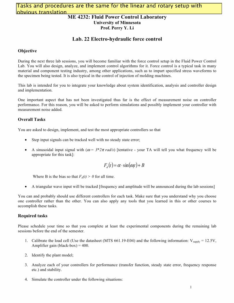
ME 4232: Fluid Power Control Laboratory University of Minnesota

Prof. Perry Y. Li

Lab. 22 Electro-hydraulic force control

Objective During the next three lab sessions, you will become familiar with the force control setup in the Fluid Power Control Lab. You will also design, analyze, and implement control algorithms for it. Force control is a typical task in many material and component testing industry, among other applications, such as to impart specified stress waveforms to the specimen being tested. It is also typical in the control of injection of molding machines. This lab is intended for you to integrate your knowledge about system identification, analysis and controller design and implementation. One important aspect that has not been investigated thus far is the effect of measurement noise on controller performance. For this reason, you will be asked to perform simulations and possibly implement your controller with measurement noise added. Overall Tasks You are asked to design, implement, and test the most appropriate controllers so that

• Step input signals can be tracked well with no steady state error;

• A sinusoidal input signal with (! = 3*2" rad/s) [tentative - your TA will tell you what frequency will be appropriate for this task]:

( ) ( ) BttFd +!= 1sin "# Where B is the bias so that Fd(t) > 0 for all time.

• A triangular wave input will be tracked [frequency and amplitude will be announced during the lab sessions]

You can and probably should use different controllers for each task. Make sure that you understand why you choose one controller rather than the other. You can also apply any tools that you learned in this or other courses to accomplish these tasks. Required tasks Please schedule your time so that you complete at least the experimental components during the remaining lab sessions before the end of the semester.

1. Calibrate the load cell (Use the datasheet (MTS 661.19-E04) and the following information: Vsupply = 12.5V, Amplifier gain (black-box) = 400.

2. Identify the plant model;

3. Analyze each of your controllers for performance (transfer function, steady state error, frequency response etc.) and stability.

4. Simulate the controller under the following situations:

2

a) Ideal plant (i.e. plant = plant model) b) Critical model parameters are ±50% c) Measurement noise (use random signal) d) Un-modeled dynamics:

( ) ( ) 22

2

nn

nmdlsim sssGsG

!!!

++"=

Where Gmdl(s) is the transfer function of your model, and !n (either 10 times or 5 times the break frequency of your plant model) is the natural frequency of the un-modeled dynamics. This for example simulates the dynamics of the bench. " = 0.5) is

5. Develop insights into how controller parameters affect the performance or stability of the system.

Demonstrate these insights by analysis if possible or otherwise by simulation results.

6. Implement your controller. If safe and appropriate, also include measurement noise in your implementation.

7. Optimize the performance of the control system by tuning the parameters. Data taking – Important You should take data AFTER you have gained sufficient understanding of the system / controller. The data that you take should be those that support your remarks / observations in your report. Thus, it is more reasonable to know what you want to say in the report first, BEFORE taking the data. This way, you can pick the most appropriate set of conditions to support your argument. Report Document your controller selection, design, analysis and implementation for various cases in the report. The report should demonstrate your understanding of both the theory and practice of control design and implementation.

m 661.19Force TransducerMTS 661.19 Force Transducers are compact, fatigue-rated devicesdesigned for measuring through-zero tension and compression loadsof 1100 to 5500 lb (5 to 25 kN).These force transducers feature

low deflection and a high degree of stiffness to give you better dynamicperformance. They also feature ahigh degree of component concen-tricity and parallelism to give yougreater accuracy during your testsetup. Accuracy is also enhanced by a shear-web design that featuresradially-oriented beams. Thesebeams compensate for off-axis loads and moments.These units are easily mounted on,

or interchanged with, existing forcetransducers on actuators, crossheads,platens or other test fixtures. They

are manufactured for long, accurateservice life using aircraft-qualitysteels, specially heat-treated to minimize distortion and ensure uni-form hardness. There are no brazedor welded joints to fatigue.MTS uses a proprietary wiring

technique to reduce electrical noise,then temperature compensates eachunit to ensure stability.You get excellent resolution and

reading accuracy from these unitsbecause of high output which issymmetrical between tension andcompression for accurate through-zero testing.In addition to single bridge models,

there are units available with dualbridges to give you the capability to continue testing should you experience any failure during testing.

F E A T U R E S

Shear Web Design!Units resist off-axis loads andmoments for greater accuracy.

Dynamic Performance!Low deflection and high stiff-ness give you better dynamicperformance.

High Output!Provides you with excellent res-olution and reading accuracy.

High Degree Of ComponentConcentricity And Parallelism!This feature gives you greateraccuracy during your test setup.

Unique Wiring Technique!A unique proprietary wiringtechnique used on the bridgeallows for minimal susceptibilityto stray magnetic fields.

661.19Force Transducer

MTS Systems Corporation14000 Technology DriveEden Prairie, MN 55344-2290952-937-4555, Fax 952-937-4515

ISO 9001:2000 CERTIFIED QMS

Specifications Subject to Change Without Notice©Copyright MTS Systems Corporation 6/1996Part Number 300140-01 661.19-02 Printed in U.S.A.

S P E C I F I C A T I O N S

Static Overload Capacity! 150% of rated force capacityTemperature Effect On Zero! 0.001% of full scale/°F! 0.002% of full scale/°CTemperature Effect On Sensitivity! 0.001% of reading/°F! 0.002% of reading/°CCompensated Temperature Range! 0°F (–18°C) to +150°F (+66°C)Useable Temperature Range! –65°F (–54°C) to +200°F (+93°C)Bridge Resistance! 350 !Maximum Excitation Voltage! 20 VdcNon-linearity! 0.08% of full scale

Threads!1/2-20 UNF-3B (M12 x 1.25mm)Hysteresis! 0.05% of full scaleRepeatability!0.03% of full scaleWeight (approximate)! 6.75 lb (3.06 kg)Calibration!Each force transducer ordered may becalibrated by MTS using our automatedcalibration system at our factory or on-site by MTS Field Service. In addition, theforce transducer and associated condi-tioning electronics may be returned toMTS for repair and recalibration.Depth

Near Side:1.00 in. (25.4 mm)Far Side:0.80 in. (20.3 mm)

ConnectorReceptaclePT02E-10-6P

2.50 in.(63.5 mm)

Force Deflection At Rated NumberModel Capacity Force Capacity Output Of Bridges

661.19E-01 1100 lb 0.001 in 1.0 mV/V Single

661.19E-02 2200 lb 0.002 in 2.0 mV/V Single

661.19E-03 3300 lb 0.001 in 1.0 mV/V Single

661.19E-04 5500 lb 0.002 in 2.0 mV/V Single

661.19E-05 1100 lb 0.001 in 1.0 mV/V Dual

661.19E-06 2200 lb 0.002 in 2.0 mV/V Dual

661.19E-07 3300 lb 0.001 in 1.0 mV/V Dual

661.19E-08 5500 lb 0.002 in 2.0 mV/V Dual

661.19F-01 5 kN 0.03 mm 1.0 mV/V Single

661.19F-02 10 kN 0.05 mm 2.0 mV/V Single

661.19F-03 15 kN 0.03 mm 1.0 mV/V Single

661.19F-04 25 kN 0.05 mm 2.0 mV/V Single

661.19F-05 5 kN 0.03 mm 1.0 mV/V Dual

661.19F-06 10 kN 0.05 mm 2.0 mV/V Dual

661.19F-07 15 kN 0.03 mm 1.0 mV/V Dual

661.19F-08 25 kN 0.05 mm 2.0 mV/V Dual

m

A B C D E F G

4.12 in. dia. 1.25 in. dia. 0.03 in. 2.62 in. 1.34 in. 0.25 in. 0.20 in. max.(104.6 mm) (31.8 mm) (0.8 mm) typ. (66.5 mm) (34.0 mm) (6.4 mm) (5.1 mm)

A

BC

D

EF G