learning guidance rewards with trajectory-space smoothing
TRANSCRIPT
Learning Guidance Rewards with Trajectory-spaceSmoothing
Tanmay GangwaniDept. of Computer Science
Yuan ZhouDept. of ISE
Jian PengDept. of Computer Science
Abstract
Long-term temporal credit assignment is an important challenge in deep rein-forcement learning (RL). It refers to the ability of the agent to attribute actions toconsequences that may occur after a long time interval. Existing policy-gradientand Q-learning algorithms typically rely on dense environmental rewards thatprovide rich short-term supervision and help with credit assignment. However,they struggle to solve tasks with delays between an action and the correspondingrewarding feedback. To make credit assignment easier, recent works have proposedalgorithms to learn dense guidance rewards that could be used in place of the sparseor delayed environmental rewards. This paper is in the same vein – starting with asurrogate RL objective that involves smoothing in the trajectory-space, we arriveat a new algorithm for learning guidance rewards. We show that the guidancerewards have an intuitive interpretation, and can be obtained without training anyadditional neural networks. Due to the ease of integration, we use the guidancerewards in a few popular algorithms (Q-learning, Actor-Critic, Distributional-RL)and present results in single-agent and multi-agent tasks that elucidate the benefitof our approach when the environmental rewards are sparse or delayed 1.
1 Introduction
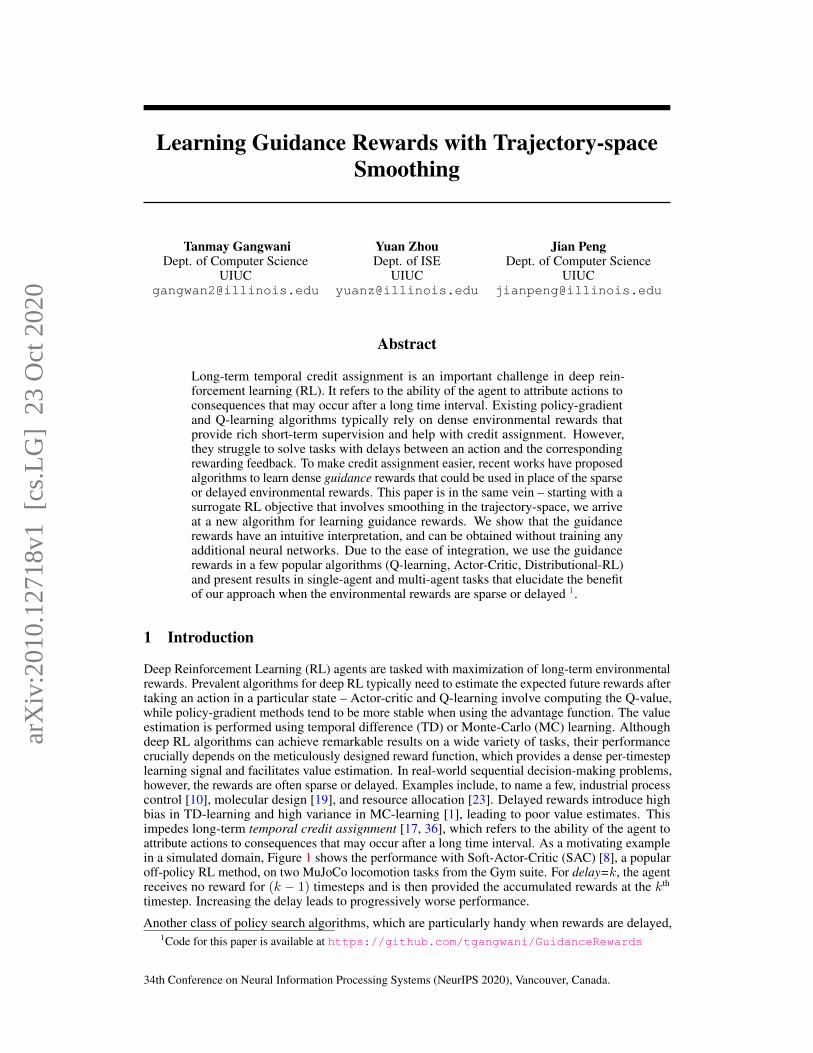
Deep Reinforcement Learning (RL) agents are tasked with maximization of long-term environmentalrewards. Prevalent algorithms for deep RL typically need to estimate the expected future rewards aftertaking an action in a particular state – Actor-critic and Q-learning involve computing the Q-value,while policy-gradient methods tend to be more stable when using the advantage function. The valueestimation is performed using temporal difference (TD) or Monte-Carlo (MC) learning. Althoughdeep RL algorithms can achieve remarkable results on a wide variety of tasks, their performancecrucially depends on the meticulously designed reward function, which provides a dense per-timesteplearning signal and facilitates value estimation. In real-world sequential decision-making problems,however, the rewards are often sparse or delayed. Examples include, to name a few, industrial processcontrol [10], molecular design [19], and resource allocation [23]. Delayed rewards introduce highbias in TD-learning and high variance in MC-learning [1], leading to poor value estimates. Thisimpedes long-term temporal credit assignment [17, 36], which refers to the ability of the agent toattribute actions to consequences that may occur after a long time interval. As a motivating examplein a simulated domain, Figure 1 shows the performance with Soft-Actor-Critic (SAC) [8], a popularoff-policy RL method, on two MuJoCo locomotion tasks from the Gym suite. For delay=k, the agentreceives no reward for (k − 1) timesteps and is then provided the accumulated rewards at the kth
timestep. Increasing the delay leads to progressively worse performance.
Another class of policy search algorithms, which are particularly handy when rewards are delayed,1Code for this paper is available at https://github.com/tgangwani/GuidanceRewards
34th Conference on Neural Information Processing Systems (NeurIPS 2020), Vancouver, Canada.
arX
iv:2
010.
1271
8v1
[cs
.LG
] 2
3 O
ct 2
020

Figure 1: Effect of delayed rewards
is black-box stochastic-optimization; examples include Evolu-tion Strategies [26] and Deep-Neuroevolution [34]. They areinvariant to delayed rewards since the trajectories are not decom-posed into individual timesteps for learning; rather zeroth-orderfinite-difference or gradient-free methods are used to learn poli-cies based only on the trajectory returns (or aggregated rewards).However, one downside is that discarding the temporal struc-ture of the RL problem leads to inferior sample-efficiency whencompared with the standard RL algorithms. Our goal in thispaper is to design an approach that easily integrates into theexisting RL algorithms, thus enjoying the sample-efficiency benefits, while being invariant to delayedrewards. To achieve this, we introduce a surrogate RL objective that involves smoothing in thetrajectory-space and arrive at a new algorithm for learning guidance rewards. The guidance rewardsare curated using only the trajectory returns and are easily inferred for each state-action tuple. Thedense supervision from the guidance rewards makes value estimation and credit assignment easier,substantially accelerating learning when the original environmental rewards are sparse or delayed.
We provide an intuitive understanding for the guidance rewards in terms of uniform credit assignment– they characterize a uniform redistribution of the trajectory return to each constituent state-action pair.A favorable property of our approach is that no additional neural networks need to be trained to obtainthe guidance rewards, unlike recent works that also examine RL with delayed rewards (c.f. Section 5).For quantitative evaluation, we combine the guidance rewards with a variety of RL algorithms andenvironments. These include single-agent tasks: Q-learning [37] in a discrete grid-world and SAC oncontinuous control locomotion tasks; and multi-agent tasks: TD3 [5] and Distributional-RL [2] inmulti-particle cooperative environments.
2 Background and Notations
Our RL environment is modeled as an infinite-horizon, discrete-time Markov Decision Process(MDP). The MDP is characterized by the tuple (S, A, r, p, γ), where S and A are the state- andaction-space, respectively, and γ ∈ [0, 1) is the discount factor. Given an action at, the next state issampled from the transition dynamics distribution, st+1 ∼ p(st+1|st, at), and the agent receives areward r(st, at) determined by the reward function r : S × A → R. A stochastic policy π(at|st)defines the state-conditioned distribution over actions. τ denotes a trajectory {s0, a0, s1, a1, . . . }and R(τ) is the sum of discounted rewards over the trajectory, R(τ) =
∑∞t=0 γ
tr(st, at). The RLobjective is to learn π that maximizes the expected R(τ), η(π) = Ep,π[R(τ)].
Actor-critic Algorithms. These methods use a critic for value function estimation and an actor thatis updated based on the information provided by the critic. The critic is trained with TD-learning in apolicy-evaluation step; then the actor is updated with an approximate gradient in the direction of policyimprovement. Under certain conditions, their repeated application converges to an optimal policy [35].We briefly outline two model-free off-policy actor-critic RL algorithms that work extremely well onhigh-dimensional tasks and are used in this paper – TD3 and SAC. TD3 is a deterministic policygradient algorithm (DPG) [29]. It uses a deterministic policy µθ that is updated with the policygradient: ∇θEs∼ρβ [Qµ(s, µθ(s))], where ρβ is the state distribution of a behavioral policy β, and Qµis the state-action value trained with the Bellman error. TD3 alleviates the Q-function overestimationbias in DPG by using Clipped Double Q-learning when calculating the Bellman target. Differently,SAC optimizes for the maximum entropy RL objective, Eπ[
∑t γ
t(r(st, at) + αH(π(·|st)))], whereH and α are the policy entropy and the temperature, respectively. SAC alternates between soft policyevaluation, which estimates the soft Q-function using a modified Bellman operator, and soft policyimprovement, which updates the actor by minimizing the Kullback-Leibler divergence between thepolicy distribution and exponential form of the soft Q-function. The loss functions for the critic (Qφ),the actor (πθ) and the temperature (α) are:
JQ(φ; r) = E(s,a,s′)∼Da′∼πθ(·|s′)
[12
(Qφ(s, a)− (r(s, a) + γ(Qφ(s′, a′)− α log πθ(a
′|s′))))2]
(1)
Jπ(θ) = E s∼Da∼πθ(·|s)
[α log(πθ(a|s))−Qφ(s, a)
]; J(α) = E s∼D
a∼πθ(·|s)
[−α log πθ(a|s)−αH
](2)
where D is the replay buffer, Qφ is the target critic network, and H is the expected target entropy.
2

3 Method
This section begins with the definition of our modified RL objective that involves smoothing in thetrajectory-space, following which we make design choices that result in guidance rewards. Givena policy πθ, the standard RL objective is: arg maxθ Eτ∼π(θ)[R(τ)]. As motivated before, withdelayed environmental rewards, directly optimizing this objective hinders learning due to difficultyin temporal credit assignment caused by value estimation errors. Objective function smoothing haslong been studied in the stochastic optimization literature. In the context of RL, Salimans et al. [26]proposed Evolution Strategies (ES) for policy search. ES creates a smoothed version of the standardRL objective using parameter-level smoothing (usually Gaussian blurring):
ηES(πθ) = Eε∼N (0,I)Eτ∼π(θ+σ·ε)[R(τ)]
where σ controls the level of smoothing. Although ES is invariant to delayed rewards, eschewing thetemporal structure of the RL problem often results in low sample efficiency. Following the broadprinciple of using a smoothed objective to obtain effective gradient signals, we consider explicitsmoothing in the trajectory-space, rather than the parameter-space. We define our maximizationobjective as:
ηsmooth(πθ) = Eτ∼π(θ)
[Eτ∼Mτ
[R(τ)]]
(3)where Mτ (τ) is the smoothing distribution over trajectories τ that is parameterized by the referencetrajectory τ . When M is a delta distribution, i.e., Mτ (τ) = δ(τ = τ), the original RL objectiveis recovered. We wish to design a smoothing distribution M that helps with credit assignment.Let β(a|s) denote a behavioral policy and the trajectory distribution induced by β in the MDP bepβ(τ) = p(s0)
∏∞t=0 p(st+1|st, at)β(at|st). Further, we introduce pβ(τ ; s, a) as the distribution
over the β-induced trajectories which include the state-action pair (s, a):
pβ(τ ; s, a)def=
pβ(τ)1[(s, a) ∈ τ ]∫τpβ(τ)1[(s, a) ∈ τ ] dτ
where 1 is the indicator function. For consistency, we require that the normalization constant bepositive ∀(s, a). Let {st, at} be the reference state-action pairs in the reference trajectory τ . Wepropose the following infinite mixture model for the smoothing distribution Mτ (τ):
Mτ ,β(τ) = (1− γ)
∞∑t=0
γtpβ(τ ; st, at)
Given a reference trajectory τ , this distribution samples trajectories from the behavioral policy βthat intersect or overlap with the reference trajectory, with intersections at later timesteps discountedexponentially with the factor γ. Inserting this in Equation 3, rearranging and ignoring constants, thesmoothed objective to maximize becomes:
ηsmooth(πθ) = Eτ∼π(θ)
[ ∞∑t=0
γt∫τ
pβ(τ ; st, at)R(τ) dτ︸ ︷︷ ︸rg(st,at)
](4)
This is equivalent to the standard RL objective, albeit with a different reward function than the envi-ronmental reward. We define this as the guidance reward function, rg(s, a;β) = Eτ∼pβ(τ ;s,a)[R(τ)].The guidance reward apportioned to each state-action pair is the expected value (under pβ) of thereturns of the trajectories which include that state-action pair. Useful features of rg are that it providesa dense reward signal, and is invariant to delays in the environmental rewards since it depends on thetrajectory return. Thus, it potentially promotes better value estimation and credit assignment.
Interpretation as uniform credit assignment. Temporal Credit assignment deals with the question:"given a final outcome (e.g. trajectory returns), how relevant was each state-action pair in thattrajectory towards achieving the return?". Prior work has proposed learning estimators that explicitlymodel the relevance of an action to future returns, or using contribution analysis methods to redis-tribute rewards to the individual timesteps (c.f. Section 5). Our method could be viewed as performinga simple redistribution – it uniformly distributes the trajectory return among the state-action pairs inthat trajectory. 2 This non-committal or maximum entropy credit assignment is natural to consider in
2In Equation 4, we excluded the constant (1− γ) from the smoothing distribution Mτ (τ) to reduce clutter.Since 1/(1− γ) is the effective horizon, (1− γ)R(τ) represents a uniform redistribution of the trajectory returnto each constituent state-action pair.
3

(a) Quiver plots during training(b) Performance withguidance rewards
Figure 2: We consider a 50× 50 grid-world with the start and goal locations marked in the image. The rewardsare episodic – a non-zero reward is only provided at the end of the episode (horizon=150 steps) and is equal tothe negative of the distance of the final position to the goal. We run for 15k episodes. The three quiver plots (leftto right) are taken after 100 episodes, 2k episodes and 15k episodes, respectively. In each quiver plot, an arrowin a state represents the guidance reward: the direction denotes the action with maximum guidance reward, i.e.,arg maxa rg(s, a), and the length denotes its magnitude in [0, 1]. A state with no arrow mean that the guidancereward is 0 for all actions in that state. For ease of exposition, we have colored all arrows pointing up/right withred and all arrows pointing down/left with blue. We note that over time, reasonable guidance rewards emergealong the diagonal path from the start location to the goal. Although the guidance rewards in the top-left andbottom-right regions of the grid are imprecise, they are not critical for learning the optimal policy to achieve thetask. Figure (right) compares tabular Q-learning with environmental rewards and our guidance rewards. Quiverplots best viewed when digitally zoomed.
the absence of any prior structure or information. The guidance reward for each state-action pair isthen obtained as the expected value (under pβ) of the uniform credit it receives from the differenttrajectory returns. For clarity of exposition, Appendix A.3 demonstrates the guidance rewards usingsome elementary MDPs and pβ .
3.1 Integrating guidance rewards into existing RL algorithms
Without access to the true MDP reward function, it is infeasible to solve for the guidance rewardsexactly. Hence, we resort to a Monte-Carlo (MC) estimation for the expectation, rg(s, a;β) =Eτ∼pβ(τ ;s,a)[R(τ)]. Let Γ denote a fixed set of trajectories generated in the MDP using β. The MCestimate can be written as: rg(s, a) = (1/N(s, a))
∑τ∈Γ
[R(τ)1[(s, a) ∈ τ ]
], where N(s, a) is the
number of trajectories in Γ which include the tuple (s, a). Please see Appendix A.1 for details onachieving the MC estimate from the smoothed RL objective (Equation 4). It is possible to deployan exploratory behavioral policy β to obtain the set Γ in a pre-training phase. Following that, thestationary guidance rewards computed from Γ could be used to learn a new policy with any of thestandard RL methods. One issue with this sequential approach is that it is challenging to designβ such that it achieves adequate state-action-space coverage in high dimensions. Perhaps moreimportantly, it is typically unnecessary to have good estimates for the guidance rewards for the entirestate-action-space. For instance, in a grid-world, if the goal location is always to the right of thestarting position of the agent, it is acceptable to have imprecise guidance reward in the left half of thegrid, as long as the agent is discouraged from venturing to the left. Therefore, we propose an iterativeapproach where the experience gathered thus far by the agent is used to build the guidance rewards,i.e., rg(s, a) is the expected value of the uniform credit received by (s, a) from the trajectoriesalready rolled out in the MDP. Simultaneously, a policy π (or Q-function) is learned using thesenon-stationary rewards. With this procedure, β could be thought of as being implicitly defined as amixture of current and past policies π. The scale of the credit apportioned to a state-action pair froma trajectory depends on the scale of its return value. For the guidance rewards to be effective, it issufficient that the relative values of the rewards be properly aligned to solve the task. Therefore, whenassigning credits, we normalize the trajectory returns to [0, 1] using min-max normalization. We referto our approach for producing guidance rewards as Iterative Relative Credit Refinement (IRCR).The guidance rewards are adapted over time as the average credit assigned to each state-action pair isrefined by the information (return value) from newly sampled trajectories.
4

Algorithm 1: Tabular Q-learning with IRCR1 Initialize Q(s,a)← 02 Rmax ← −∞; Rmin ←∞ . Maximum/Minimum return thus far3 B(s, a)← ∅ ∀ (s, a) . Buffer that stores for each (s, a), a list of returns of trajectories that include
that (s, a)
4 Function GetGuidanceReward(s, a):/* Get normalized returns; return 0 if B(s, a) = ∅ */
5 return ERi∼B(s,a)[Ri−RminRmax−Rmin
]
6 for each episode do7 Re ← 0 . Accumulates rewards for current episode8 τe ← ∅ . Stores state-action pairs for current episode
9 for each step in {1, . . . , T} do10 Choose a from s using policy derived from Q (ε-greedy)11 Take action a and observe r, s′ . Sample transition from the environment12 τe ← τe ∪ {(s,a)}; Re ← Re + r13 rg(s,a)← GetGuidanceReward(s,a)14 Q(s,a)← Q(s,a) + α [rg(s,a) + γ maxa′ Q(s′,a′) - Q(s,a)]15 end16 for each (s,a) in τe do17 B(s, a)← B(s, a) ∪ {Re} . Update B for (s, a) along the collected trajectory18 end19 Rmax ← max(Rmax, Re); Rmin ← min(Rmin, Re) . Update Rmax, Rmin
20 end
Any standard RL algorithm could be modified by replacing the environmental rewards with theguidance rewards. In Algorithm 1, we outline this for tabular Q-learning with small state and actionspaces. The notable change from the standard Q-learning is the use of rg in Line 14, instead of theenvironmental reward. To compute rg, we maintain a buffer B(s, a) for each state-action pair thatstores the returns of the past trajectories which include that state-action pair (Line 17). The guidancerewards evolve over time since the average credit allotted to a state-action pair changes as moreexperience is gathered in the MDP. To illustrate this, we run Algorithm 1 in a 50× 50 grid-world withepisodic environmental rewards. Figure 2a provides some insights on the structure of the guidancerewards assigned to the different regions of the grid as training progresses; the description of theepisodic rewards and the arrows in the quiver plots is provided in the figure caption. In Figure 2b, weshow the performance gains compared with tabular Q-learning using environmental rewards. Pleasesee Appendix A.2 for hyperparameters and other details.
Scaling to high-dimensional continuous spaces. Actor-critic algorithms that scale to more complexenvironments (e.g. TD3, SAC) maintain an experience replay buffer [14] that stores {s, a, s′, r}tuples. These algorithms can be readily tailored to use guidance rewards. In Algorithm 2, wesummarize SAC with IRCR. The environmental reward in the experience replay tuple is replaced withthe return of the trajectory which produced that tuple (Line 13). When computing the soft Bellmanerror for learning the soft Q-function, the guidance reward is calculated by normalizing this returnvalue (Lines 18-19). Mathematically, this is equivalent to the MC estimation of the guidance rewardusing a single trajectory, rather than the expected credit from a trajectory distribution. This is not anissue in practice if the soft Q-function, which is learned with these guidance rewards, is parameterizedby a deep neural network that tends to generalize well in the vicinity of the input data. Indeed, as ourexperiments will show, Algorithm 2 achieves reliable performance in high-dimensional tasks. Otheractor-critic algorithms could be modified analogously to incorporate the guidance rewards.
Convergence. Some comments are in order concerning the convergence of our iterative approach.We provide a qualitative analysis by drawing an analogy with the Cross Entropy (CE) method [16, 25].For policy search, CE uses a multivariate Gaussian distribution to represent a population of policies.In each iteration, individuals πk are drawn from this distribution, their fitness, Eτ∼πk [R(τ)], isevaluated, and a fixed number of fittest individuals determine the new mean and variance of thepopulation. This fitness-based selection ensures steady policy improvement. In IRCR, the trajectories
5

Algorithm 2: Soft Actor-Critic with IRCR1 Initialize φ, φ, θ . Policy and critic parameters2 Rmax ← −∞; Rmin ←∞ . Maximum/Minimum return thus far3 D ← ∅ . Empty replay buffer
4 for each episode do5 Re ← 0 . Accumulates rewards for current episode6 De ← ∅ . Stores transitions for current episode
7 for each step in {1, . . . , T} do8 a ∼ πθ(a|s)9 Take action a and observe r, s′ . Sample transition from the environment
10 De ← De ∪ {(s,a, s′)}; Re ← Re + r11 end
12 for each (s, a, s′) ∈ De do13 D ← D ∪ {(s, a, s′, Re)} . Append each transition with Re and add to replay buffer14 end15 Rmax ← max(Rmax, Re); Rmin ← min(Rmin, Re) . Update Rmax, Rmin
16 for each gradient step do17 {s(k), a(k), s′(k), R(k)}k∈N+ ∼ D . Sample batch
18 r(k)g ← R(k)−Rmin
Rmax−Rmin. Get guidance reward by normalizing return
19 φ← φ− λ∇φJQ(φ; rg) . Update Q-function using guidance rewards, (Eq. 1)20 θ ← θ − λ∇θJπ(θ); α← α− λ∇αJ(α) . Update policy and temperature, (Eq. 2)21 end22 end
generated by a mixture of the current and past policies (π0:i) are used to compute the guidancerewards (rg); πi+1 is then obtained by a policy optimization step with these rewards. Since rg ispositively correlated with the environmental returns R(τ), maximizing for a discounted sum of rgtends to seek out a policy that attains higher R(τ) compared to π0:i, on average. Consequently, thisoptimization step facilitates policy improvement in the same spirit as the CE method. The next sectionprovides empirical evidence that the policy behavior improves over iterations of IRCR. We considerthe theoretical study of convergence as an important future work.
4 Experiments
This section evaluates our approach on various single-agent and multi-agent RL tasks to quantifythe benefits of using the guidance rewards in place of the environmental rewards, when the latter aresparse or delayed.
4.1 Single-agent environments and baselines
We benchmark high-dimensional, continuous-control locomotion tasks based on the MuJoCo physicssimulator, provided in OpenAI Gym [3]. We compare SAC (IRCR) outlined in Algorithm 2 with thefollowing baselines:
• SAC with environmental rewards. It uses the same hyperparameters as SAC (IRCR). Please seeAppendix A.2 for details.
• Generative Adversarial Self-imitation Learning (GASIL), which represents the method proposedin Guo et al. [7]; Gangwani et al. [6]. A buffer stores the top-k trajectories according to thereturn. A discriminator network, which is a binary classifier that distinguishes the buffer datafrom data generated by the current policy, acts as a source of the guidance rewards.
• Reward Regression, which typifies the approaches presented in Arjona-Medina et al. [1]; Liuet al. [15]. They formulate a regression task that predicts the return given the entire trajectory.A network trained with this regression loss helps to decompose the trajectory return back tothe constituent state-action pairs, and provides the guidance rewards. We include the resultsfrom Liu et al. [15] using the Transformer architecture (data obtained from authors).
6
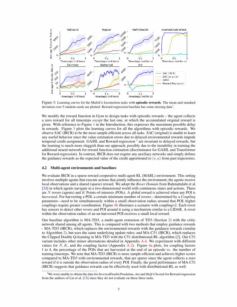
Figure 3: Learning curves for the MuJoCo locomotion tasks with episodic rewards. The mean and standarddeviation over 5 random seeds are plotted. Reward-regression baseline has some missing data3.
We modify the reward function in Gym to design tasks with episodic rewards – the agent collectsa zero reward for all timesteps except the last one, at which the accumulated original reward isgiven. With reference to Figure 1 in the Introduction, this expresses the maximum possible delayin rewards. Figure 3 plots the learning curves for all the algorithms with episodic rewards. Weobserve SAC (IRCR) to be the most sample-efficient across all tasks. SAC (original) is unable to learnany useful behavior since the value estimation errors due to delayed environmental rewards impedetemporal credit assignment. GASIL and Reward-regression 3 are invariant to delayed rewards, butthe learning is much more sluggish than our approach, possibly due to the instability in training theadditional neural network for reward function estimation (discriminator for GASIL and Transformerfor Reward-regression). In contrast, IRCR does not require any auxiliary networks and simply definesthe guidance rewards as the expected value of the credit apportioned to (s, a) from past trajectories.
4.2 Multi-agent environments and baselines
We evaluate IRCR in a sparse-reward cooperative multi-agent RL (MARL) environment. This settinginvolves multiple agents that execute actions that jointly influence the environment; the agents receivelocal observations and a shared (sparse) reward. We adopt the Rover Domain from Rahmattalabi et al.[24] in which agents navigate in a two-dimensional world with continuous states and actions. Thereare N rovers (agents) and K Points-of-interests (POIs). A global reward is achieved when any POI isharvested. For harvesting a POI, a certain minimum number of rovers—determined by a Couplingparameter—need to be simultaneously within a small observation radius around that POI; highercouplings require greater coordination. Figure 4b illustrates a scenario with coupling=2. Each roverhas sensors to detect other rovers and POI around it using a mechanism similar to a LIDAR. A roverwithin the observation radius of an un-harvested POI receives a small local reward.
Our baseline algorithm is MA-TD3, a multi-agent extension of TD3 (Section 2) with the criticnetwork shared among all agents. This is compared with two methods that employ guidance rewards– MA-TD3 (IRCR), which replaces the environmental rewards with the guidance rewards (similarto Algorithm 2), but uses the same underlying update rules; and MA-C51 (IRCR), which replacesthe Clipped Double Q-learning in MA-TD3 with the C51 distributional-RL algorithm [2]. Our C51variant includes other minor alternations detailed in Appendix A.4. We experiment with differentvalues for N,K, and the coupling factor (Appendix A.2). Figure 4a plots, for coupling factors1 to 4, the percentage of the POIs that are harvested at the end of an episode vs. the number oftraining timesteps. We note that MA-TD3 (IRCR) is more sample-efficient and achieves higher scorescompared to MA-TD3 with environmental rewards, that are sparse since the agent collects a zeroreward if it is outside the observation radius of every POI. Finally, the good performance of MA-C51(IRCR) suggests that guidance rewards can be effectively used with distributional-RL as well.
3We were unable to obtain the data for InvertedDoublePendulum, Ant and Half-Cheetah for Reward-regressionfrom the authors of Liu et al. [15] since they do not evaluate on these three tasks.
7
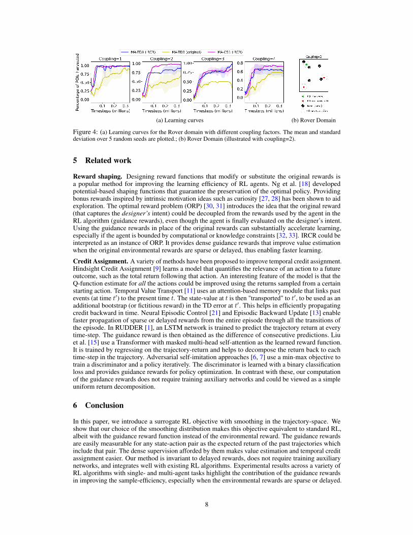
(a) Learning curves (b) Rover Domain
Figure 4: (a) Learning curves for the Rover domain with different coupling factors. The mean and standarddeviation over 5 random seeds are plotted.; (b) Rover Domain (illustrated with coupling=2).
5 Related work
Reward shaping. Designing reward functions that modify or substitute the original rewards isa popular method for improving the learning efficiency of RL agents. Ng et al. [18] developedpotential-based shaping functions that guarantee the preservation of the optimal policy. Providingbonus rewards inspired by intrinsic motivation ideas such as curiosity [27, 28] has been shown to aidexploration. The optimal reward problem (ORP) [30, 31] introduces the idea that the original reward(that captures the designer’s intent) could be decoupled from the rewards used by the agent in theRL algorithm (guidance rewards), even though the agent is finally evaluated on the designer’s intent.Using the guidance rewards in place of the original rewards can substantially accelerate learning,especially if the agent is bounded by computational or knowledge constraints [32, 33]. IRCR could beinterpreted as an instance of ORP. It provides dense guidance rewards that improve value estimationwhen the original environmental rewards are sparse or delayed, thus enabling faster learning.
Credit Assignment. A variety of methods have been proposed to improve temporal credit assignment.Hindsight Credit Assignment [9] learns a model that quantifies the relevance of an action to a futureoutcome, such as the total return following that action. An interesting feature of the model is that theQ-function estimate for all the actions could be improved using the returns sampled from a certainstarting action. Temporal Value Transport [11] uses an attention-based memory module that links pastevents (at time t′) to the present time t. The state-value at t is then "transported" to t′, to be used as anadditional bootstrap (or fictitious reward) in the TD error at t′. This helps in efficiently propagatingcredit backward in time. Neural Episodic Control [21] and Episodic Backward Update [13] enablefaster propagation of sparse or delayed rewards from the entire episode through all the transitions ofthe episode. In RUDDER [1], an LSTM network is trained to predict the trajectory return at everytime-step. The guidance reward is then obtained as the difference of consecutive predictions. Liuet al. [15] use a Transformer with masked multi-head self-attention as the learned reward function.It is trained by regressing on the trajectory-return and helps to decompose the return back to eachtime-step in the trajectory. Adversarial self-imitation approaches [6, 7] use a min-max objective totrain a discriminator and a policy iteratively. The discriminator is learned with a binary classificationloss and provides guidance rewards for policy optimization. In contrast with these, our computationof the guidance rewards does not require training auxiliary networks and could be viewed as a simpleuniform return decomposition.
6 Conclusion
In this paper, we introduce a surrogate RL objective with smoothing in the trajectory-space. Weshow that our choice of the smoothing distribution makes this objective equivalent to standard RL,albeit with the guidance reward function instead of the environmental reward. The guidance rewardsare easily measurable for any state-action pair as the expected return of the past trajectories whichinclude that pair. The dense supervision afforded by them makes value estimation and temporal creditassignment easier. Our method is invariant to delayed rewards, does not require training auxiliarynetworks, and integrates well with existing RL algorithms. Experimental results across a variety ofRL algorithms with single- and multi-agent tasks highlight the contribution of the guidance rewardsin improving the sample-efficiency, especially when the environmental rewards are sparse or delayed.
8

Broader Impact
In this paper, we propose techniques to improve the sample-efficiency of Reinforcement Learning(RL) algorithms when the environmental rewards are sparse or delayed. Many real-world decision-making problems of interest are of this nature – the rewarding (or penalizing) feedback is usuallyavailable only after a long sequence of interaction with the environment. Some prominent examplesinclude a.) Chemical Synthesis, where the product yield and the functional measurements mostlyhappen at the last step of the entire process; b.) Industrial Control Processes, which involve sequentialcalibration of many control variables to achieve the desired output, for instance, the final metal puritymetric in a metal-refining furnace operation; and c.) RL in healthcare for uncovering promisingtreatment regimes, where there could be delayed interaction between treatments and human bodies.Techniques that make RL algorithms robust in the face of delayed rewards are therefore poised tohave a hugely positive societal influence across a range of sectors. We believe our work is a step inthe direction of developing such techniques.
Acknowledgments and Disclosure of Funding
This work is supported by the National Science Foundation under grants OAC-1835669 and CCF-2006526. Yuan Zhou is supported in part by a Ye Grant and a JPMorgan Chase AI Research FacultyResearch Award.
References[1] Jose A Arjona-Medina, Michael Gillhofer, Michael Widrich, Thomas Unterthiner, Johannes
Brandstetter, and Sepp Hochreiter. Rudder: Return decomposition for delayed rewards. InAdvances in Neural Information Processing Systems, pp. 13544–13555, 2019.
[2] Marc G Bellemare, Will Dabney, and Rémi Munos. A distributional perspective on reinforce-ment learning. In Proceedings of the 34th International Conference on Machine Learning-Volume 70, pp. 449–458. JMLR. org, 2017.
[3] Greg Brockman, Vicki Cheung, Ludwig Pettersson, Jonas Schneider, John Schulman, Jie Tang,and Wojciech Zaremba. Openai gym. arXiv preprint arXiv:1606.01540, 2016.
[4] Tao Chen, Adithyavairavan Murali, and Abhinav Gupta. Hardware conditioned policies formulti-robot transfer learning. In Advances in Neural Information Processing Systems, pp.9333–9344, 2018.
[5] Scott Fujimoto, Herke van Hoof, and Dave Meger. Addressing function approximation error inactor-critic methods. arXiv preprint arXiv:1802.09477, 2018.
[6] Tanmay Gangwani, Qiang Liu, and Jian Peng. Learning self-imitating diverse policies. arXivpreprint arXiv:1805.10309, 2018.
[7] Yijie Guo, Junhyuk Oh, Satinder Singh, and Honglak Lee. Generative adversarial self-imitationlearning. arXiv preprint arXiv:1812.00950, 2018.
[8] Tuomas Haarnoja, Aurick Zhou, Pieter Abbeel, and Sergey Levine. Soft actor-critic: Off-policy maximum entropy deep reinforcement learning with a stochastic actor. arXiv preprintarXiv:1801.01290, 2018.
[9] Anna Harutyunyan, Will Dabney, Thomas Mesnard, Mohammad Gheshlaghi Azar, Bilal Piot,Nicolas Heess, Hado P van Hasselt, Gregory Wayne, Satinder Singh, Doina Precup, et al.Hindsight credit assignment. In Advances in neural information processing systems, pp. 12467–12476, 2019.
[10] Daniel Hein, Stefan Depeweg, Michel Tokic, Steffen Udluft, Alexander Hentschel, Thomas ARunkler, and Volkmar Sterzing. A benchmark environment motivated by industrial controlproblems. In 2017 IEEE Symposium Series on Computational Intelligence (SSCI), pp. 1–8.IEEE, 2017.
9

[11] Chia-Chun Hung, Timothy Lillicrap, Josh Abramson, Yan Wu, Mehdi Mirza, FedericoCarnevale, Arun Ahuja, and Greg Wayne. Optimizing agent behavior over long time scales bytransporting value. Nature communications, 10(1):1–12, 2019.
[12] Diederik P Kingma and Jimmy Ba. Adam: A method for stochastic optimization. arXiv preprintarXiv:1412.6980, 2014.
[13] Su Young Lee, Choi Sungik, and Sae-Young Chung. Sample-efficient deep reinforcementlearning via episodic backward update. In Advances in Neural Information Processing Systems,pp. 2110–2119, 2019.
[14] Long-Ji Lin. Self-improving reactive agents based on reinforcement learning, planning andteaching. Machine learning, 8(3-4):293–321, 1992.
[15] Yang Liu, Yunan Luo, Yuanyi Zhong, Xi Chen, Qiang Liu, and Jian Peng. Sequence mod-eling of temporal credit assignment for episodic reinforcement learning. arXiv preprintarXiv:1905.13420, 2019.
[16] Shie Mannor, Reuven Y Rubinstein, and Yohai Gat. The cross entropy method for fast policysearch. In Proceedings of the 20th International Conference on Machine Learning (ICML-03),pp. 512–519, 2003.
[17] Marvin Minsky. Steps toward artificial intelligence. Proceedings of the IRE, 49(1):8–30, 1961.
[18] Andrew Y Ng, Daishi Harada, and Stuart Russell. Policy invariance under reward transforma-tions: Theory and application to reward shaping. In ICML, volume 99, pp. 278–287, 1999.
[19] Marcus Olivecrona, Thomas Blaschke, Ola Engkvist, and Hongming Chen. Molecular de-novodesign through deep reinforcement learning. Journal of cheminformatics, 9(1):48, 2017.
[20] Matthias Plappert, Rein Houthooft, Prafulla Dhariwal, Szymon Sidor, Richard Y Chen, Xi Chen,Tamim Asfour, Pieter Abbeel, and Marcin Andrychowicz. Parameter space noise for exploration.arXiv preprint arXiv:1706.01905, 2017.
[21] Alexander Pritzel, Benigno Uria, Sriram Srinivasan, Adria Puigdomenech Badia, Oriol Vinyals,Demis Hassabis, Daan Wierstra, and Charles Blundell. Neural episodic control. In Proceedingsof the 34th International Conference on Machine Learning-Volume 70, pp. 2827–2836. JMLR.org, 2017.
[22] Yu Qiao and Nobuaki Minematsu. A study on invariance of f -divergence and its application tospeech recognition. IEEE Transactions on Signal Processing, 58(7):3884–3890, 2010.
[23] Hazhir Rahmandad, Nelson Repenning, and John Sterman. Effects of feedback delay onlearning. System Dynamics Review, 25(4):309–338, 2009.
[24] Aida Rahmattalabi, Jen Jen Chung, Mitchell Colby, and Kagan Tumer. D++: Structural creditassignment in tightly coupled multiagent domains. In 2016 IEEE/RSJ International Conferenceon Intelligent Robots and Systems (IROS), pp. 4424–4429. IEEE, 2016.
[25] Reuven Y Rubinstein and Dirk P Kroese. The cross-entropy method: a unified approach tocombinatorial optimization, Monte-Carlo simulation and machine learning. Springer Science& Business Media, 2013.
[26] Tim Salimans, Jonathan Ho, Xi Chen, and Ilya Sutskever. Evolution strategies as a scalablealternative to reinforcement learning. arXiv preprint arXiv:1703.03864, 2017.
[27] Jürgen Schmidhuber. A possibility for implementing curiosity and boredom in model-buildingneural controllers. In Proc. of the international conference on simulation of adaptive behavior:From animals to animats, pp. 222–227, 1991.
[28] Jürgen Schmidhuber. Artificial curiosity based on discovering novel algorithmic predictabilitythrough coevolution. In Proceedings of the 1999 Congress on Evolutionary Computation-CEC99(Cat. No. 99TH8406), volume 3, pp. 1612–1618. IEEE, 1999.
10
[29] David Silver, Guy Lever, Nicolas Heess, Thomas Degris, Daan Wierstra, and Martin Riedmiller.Deterministic policy gradient algorithms. 2014.
[30] Satinder Singh, Richard L Lewis, and Andrew G Barto. Where do rewards come from. InProceedings of the annual conference of the cognitive science society, pp. 2601–2606. CognitiveScience Society, 2009.
[31] Satinder Singh, Richard L Lewis, Andrew G Barto, and Jonathan Sorg. Intrinsically motivatedreinforcement learning: An evolutionary perspective. IEEE Transactions on Autonomous MentalDevelopment, 2(2):70–82, 2010.
[32] Jonathan Sorg, Satinder P Singh, and Richard L Lewis. Internal rewards mitigate agentboundedness. In Proceedings of the 27th international conference on machine learning (ICML-10), pp. 1007–1014, 2010.
[33] Jonathan Sorg, Satinder Singh, and Richard L Lewis. Optimal rewards versus leaf-evaluationheuristics in planning agents. In Twenty-Fifth AAAI Conference on Artificial Intelligence, 2011.
[34] Felipe Petroski Such, Vashisht Madhavan, Edoardo Conti, Joel Lehman, Kenneth O Stanley, andJeff Clune. Deep neuroevolution: Genetic algorithms are a competitive alternative for trainingdeep neural networks for reinforcement learning. arXiv preprint arXiv:1712.06567, 2017.
[35] Richard S Sutton and Andrew G Barto. Reinforcement learning: An introduction. MIT press,2018.
[36] Richard Stuart Sutton. Temporal credit assignment in reinforcement learning. 1984.
[37] Christopher JCH Watkins and Peter Dayan. Q-learning. Machine learning, 8(3-4):279–292,1992.
[38] Manzil Zaheer, Satwik Kottur, Siamak Ravanbakhsh, Barnabas Poczos, Russ R Salakhutdinov,and Alexander J Smola. Deep sets. In Advances in neural information processing systems, pp.3391–3401, 2017.
11

A Appendix: Learning Guidance Rewards withTrajectory-space Smoothing
A.1 Monte-Carlo Estimate of the Guidance Rewards
ηsmooth(πθ) = Eτ∼π(θ)
[ ∞∑t=0
γtEτ∼pβ(τ ;s,a)[R(τ)]]; pβ(τ ; s, a)
def=
pβ(τ)1[(s, a) ∈ τ ]∫τpβ(τ)1[(s, a) ∈ τ ] dτ
Let ρπ(s, a) denote the unnormalized discounted state-action visitation distribution for π. Then:
ηsmooth(πθ) = E(s,a)∼ρπEτ∼pβ(τ ;s,a)[R(τ)]
Plugging in the definition of pβ(τ ; s, a) and using linearity of expectations:
ηsmooth(πθ) = Eτ∼pβ(τ)E(s,a)∼ρπ
[R(τ)1[(s, a) ∈ τ ]∫
τpβ(τ)1[(s, a) ∈ τ ] dτ
]
Let Γ denote a set of N trajectories generated in the MDP using β, and N(s, a) be the count of thetrajectories which include the tuple (s, a). The Monte-Carlo estimate of ηsmooth(πθ) is:
ηsmooth(πθ) =1
N
∑τ∈Γ
E(s,a)∼ρπ
[R(τ)1[(s, a) ∈ τ ]
N(s, a)/N
]
= E(s,a)∼ρπ
∑τ∈Γ
[R(τ)1[(s, a) ∈ τ ]
N(s, a)
]︸ ︷︷ ︸
rg(s,a)
where rg(s, a) is same as the Monte-Carlo estimate of the guidance rewards defined in Section 3.1.We further define rg(s, a) = 0 if N(s, a) = 0.
A.2 Implementation Details and Hyperparameters
Tabular Q-learning
Table 1 provides the hyperparameters for the Tabular Q-learning experiment in a 50 × 50 grid-world with episodic environmental rewards (Figure 2). Both IRCR and the baseline share the samehyperparameters.
Hyperparameter Valuelearning rate 0.3 at start, linearly annealedexploration ε-greedy (ε = 0.5 at start, linearly annealed)discount (γ) 0.9
episode horizon 150 steps# training episodes 15000
Table 1: Hyper-parameters for Tabular Q-learning
SAC
Table 2 provides the hyperparameters for SAC (Algorithm 2) which is used for the experiments inFigure 3. For the experience replay, the usual FIFO buffer is augmented with a small Min-Heapbuffer which stores a few high return past episodes (details in Table). This is used in all the baselinesas well. Both SAC (IRCR) and SAC (original) share the same hyperparameters.
12

Hyperparameter Value# hidden layers (all networks) 2
# hidden units per layer 256# samples per minibatch 256
nonlinearity ReLUoptimizer Adam [12]
discount (γ) 0.99entropy target −|A|
target smoothing coefficient 0.001learning rate 1× 10⁻⁴ for policy and temperature, 3× 10⁻⁴ for criticreplay buffer 3× 10⁵ transitions (FIFO) + 10 episodes (Min Heap)
Table 2: Hyper-parameters for SAC
MA-TD3
Since our multi-agent task is cooperative and involves maximization of a scalar team reward, we use asingle critic network that is shared amongst the agents. Furthermore, as the agents are homogeneous(same observation- and action-space), we design a permutation-invariant critic:
Q(s,a) = g(mean({f(o1, a1), . . . , f(ok, ak)}))where (oi, ai) are the local observation and action of agent i, (s,a) denote joint observations andactions, and g, f are neural networks. This permutation invariant set representation was proposedby Zaheer et al. [38]. Table 3 provides the hyperparameters for MA-TD3 which is used for the exper-iments in Figure 4a. Both MA-TD3 (IRCR) and MA-TD3 (original) share the same hyperparameters.
Hyperparameter Valuepolicy architecture 2 hidden layers, 128 hidden unitscritic architecture shared, permutation-invariant (described above)
# samples per minibatch 256nonlinearity Tanhoptimizer Adam [12]
discount (γ) 0.99target smoothing coefficient 0.005
episode horizon 100 stepslearning rate 1× 10⁻⁴ for policy, 3× 10⁻⁴ for criticreplay buffer 5× 10⁴ transitions (FIFO) + 100 episodes (Min Heap)
exploration strategy N (0, 0.1) + Adaptive Parameter Noise [20]
Table 3: Hyper-parameters for MA-TD3
The following are the specifics for the environments used in Figure 4a:
• Coupling=1. # POIs = 3, # Agents = 3• Coupling=2. # POIs = 4, # Agents = 4• Coupling=3. # POIs = 4, # Agents = 6• Coupling=4. # POIs = 4, # Agents = 8
A.3 Illustration of Guidance Rewards with Simple MDP and pβ
Consider the MDP in Figure 5 with the states {s1, s2, s3, s4}, s1 is the start state, {s3, s4} are theterminal states. {a1, a2} are the possible actions from s1; {a3, a4} are the possible actions from s2.There are 4 possible trajectories. Let the return associated with each trajectory be the following:
13
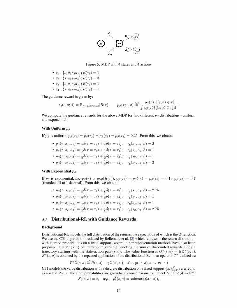
Figure 5: MDP with 4 states and 4 actions
• τ1 : {s1a1s2a3};R(τ1) = 1
• τ2 : {s1a1s2a4};R(τ2) = 3
• τ3 : {s1a2s2a3};R(τ3) = 1
• τ4 : {s1a2s2a4};R(τ4) = 1
The guidance reward is given by:
rg(s, a;β) = Eτ∼pβ(τ ;s,a)[R(τ)] pβ(τ ; s, a)def=
pβ(τ)1[(s, a) ∈ τ ]∫τpβ(τ)1[(s, a) ∈ τ ] dτ
We compute the guidance rewards for the above MDP for two different pβ distributions - uniformand exponential.
With Uniform pβ
If pβ is uniform, pβ(τ1) = pβ(τ2) = pβ(τ3) = pβ(τ4) = 0.25. From this, we obtain:
• pβ(τ ; s1, a1) = 12δ(τ = τ1) + 1
2δ(τ = τ2); rg(s1, a1;β) = 2
• pβ(τ ; s1, a2) = 12δ(τ = τ3) + 1
2δ(τ = τ4); rg(s1, a2;β) = 1
• pβ(τ ; s2, a3) = 12δ(τ = τ1) + 1
2δ(τ = τ3); rg(s2, a3;β) = 1
• pβ(τ ; s2, a4) = 12δ(τ = τ2) + 1
2δ(τ = τ4); rg(s2, a4;β) = 2
With Exponential pβ
If pβ is exponential, i.e. pβ(τ) ∝ exp(R(τ)), pβ(τ1) = pβ(τ3) = pβ(τ4) = 0.1; pβ(τ2) = 0.7(rounded off to 1 decimal). From this, we obtain:
• pβ(τ ; s1, a1) = 18δ(τ = τ1) + 7
8δ(τ = τ2); rg(s1, a1;β) = 2.75
• pβ(τ ; s1, a2) = 12δ(τ = τ3) + 1
2δ(τ = τ4); rg(s1, a2;β) = 1
• pβ(τ ; s2, a3) = 12δ(τ = τ1) + 1
2δ(τ = τ3); rg(s2, a3;β) = 1
• pβ(τ ; s2, a4) = 78δ(τ = τ2) + 1
8δ(τ = τ4); rg(s2, a4;β) = 2.75
A.4 Distributional-RL with Guidance Rewards
Background
Distributional-RL models the full distribution of the returns, the expectation of which is the Q-function.We use the C51 algorithm introduced by Bellemare et al. [2] which represents the return distributionwith learned probabilities on a fixed support; several other representation methods have also beenproposed. Let Zπ(s, a) be the random variable denoting the sum of discounted rewards along atrajectory starting with the state-action pair (s, a). The value function is Qπ(s, a) = EZπ(s, a).Zπ(s, a) is obtained by the repeated application of the distributional Bellman operator T π defined as:
T πZ(s, a)D= R(s, a) + γZ(s′, a′) s′ ∼ p(·|s, a), a′ ∼ π(·|s′)
C51 models the value distribution with a discrete distribution on a fixed support {zi}Ni=1, referred toas a set of atoms. The atom probabilities are given by a learned parametric model fθ : S ×A → RN :
Zθ(s, a) = zi w.p. piθ(s, a) = softmax(fθ(s, a))i
14
Atom Support and Guidance Rewards in Log-space
In Bellemare et al. [2], the support of the atoms ranges from Vmin to Vmax, which are environment-specific variables defining the limits of the returns possible in that environment. To make the supportrange environment-agnostic, we define it in the log-space: wi = {1/N, 2/N, . . . , 1} and zi = logwi.Thus, the Q-function is written as Qθ(s, a) =
∑i piθ(s, a) logwi.
We further define guidance rewards modified with a log function, rLg(s, a) = log rg(s, a). Recallthat rg ∈ [0, 1] due to the min-max normalization; hence the application of log is proper (expect at 0where a small ε should be added). Although this transformation changes the magnitude, the relativeordering of the guidance rewards is preserved due to the monotonicity of the log. The parametricmodel fθ is optimized with TD-learning. With the distributional Bellman equation, this is equivalentto a distribution matching problem. Given a training tuple (s, a, rLg, s
′) from the replay buffer, thediscrete target distribution is:
rLg + γzi w.p. piθ = softmax(fθ(s′, a′))i
Using the log-space atom support and definition of rLg, we can rewrite this as:
log[rg.wi
γ]
w.p. piθ = softmax(fθ(s′, a′))i
Similarly, the discrete source distribution is:
logwi w.p. piθ = softmax(fθ(s, a))i
The source and the target distributions have a support interval (-∞, 0]. In principle, any f -divergencemetric on them could be minimized. An alternative is to induce a transformation before the divergenceminimization. This is justified by the following theorem from Qiao & Minematsu [22]: "The f-divergence between two distributions is invariant under differentiable and invertible transformation".With an exponential transformation, we get the following distributions that are now shaped to have asupport interval (0,1]:
rg.wiγ w.p. piθ = softmax(fθ(s
′, a′))i
wi w.p. piθ = softmax(fθ(s, a))i
Following [2], we minimize the KL-divergence between these distributions using a projection step toaccount for the mismatch in the atom positions between the source and the target.
A.5 Discussion Points
Exploration vs. Credit-assignment. Exploration and credit assignment are two distinct fundamentalproblems in RL. The former deals with the discovery of new useful information, the latter is aboutefficiently incorporating this information for learning a robust policy. In hard exploration problems, anagent typically obtains zero rewards in each episode unless an exploration impetus is given, whereasin our setting, a reward signal is readily provided to the agent at the end of every episode. The focus,therefore, is to train effectively from this delayed feedback and improve upon the credit assignment.
Limitations of IRCR. Since the reward that the agent optimizes for is different from the original taskreward and is coupled to a behavioral policy β, for a given MDP, it might be possible to design anadversarial β such that optimizing for the resultant guidance rewards leads to unintended behaviors(as per the task rewards). Although not visible in our empirical evaluation, a limitation of IRCRis that a careful adaptation of β could be crucial in some domains to avoid this. For instance, ifβ gets stuck in some region of the state-action-space, the learning agent may also get trapped in alocal optimum due to deceptive guidance rewards. Combining IRCR with methods that explicitlyincentivize exploration is a promising approach.
A.6 Further Experiments
Robotic manipulator arm environment. Figure 6 shows the robotic arm that models a 7 degree-of-freedom Sawyer robot, inspired by Chen et al. [4]. The task is to insert a cylindrical peg (held in theend-effector attached to the arm) into a hole some distance away on the table. A non-zero reward isprovided only at the end of every episode and is equal to exponential of negative L2 distance betweenthe final position of the peg and the hole. In Table 4, we compare the final performance of the SAC
15

Figure 6: MuJoCo model of a 7 DoF armbased on the Sawyer robot.
SAC(env. rewards)
SAC(IRCR)
RandomPolicy
104±4 160±7 90±11
Table 4: SAC performance on the peg-insertion taskwith environmental and guidance rewards. Mean andstandard deviation over 5 random seeds are reported.
SAC (env. rewards)n-step returns (n=10)
SAC (env. rewards)λ-returns (λ=0.9)
TD3(env. rewards)
TD3(IRCR)
Hopper 626±281 566±101 235±37 2981±114
Half-Cheetah −42±29 −112±206 −123±50 6844±918
Table 5: Performance (mean and standard deviation over 5 random seeds) of various algorithms.
algorithm with environmental and guidance rewards, and note that the latter is considerably better.
Baselines for better reward propagation. Table 5 includes the following baselines: SAC (n-step)uses n-step returns for the Bellman error update of the soft Q-function, and SAC (λ-returns) augmentsthe Q-function training with TD(λ), which interpolates nicely between 1-step TD and MC returnsbased on the value of λ. We tested with n={3,10,20} and λ={0.5,0.9,0.95,1.0} but observe that thesemethods are unable to solve the MuJoCo locomotion tasks with episodic rewards. Our conjecturefor their low scores with episodic rewards is that the reward delay exacerbates the variance is MC,and bias in TD, to such an extent that using them separately, or mixing them via interpolation, is notsufficient to alleviate the problems in value estimation for credit assignment. IRCR takes a differentapproach of learning guidance rewards for each time-step and integrates well with 1-step TD (due tothe bias reduction afforded by the dense guidance rewards). Table 5 also contrasts TD3 (IRCR) withTD3 (environmental rewards) on the locomotion tasks.
16