learning the nonlinear geometric structure of high
TRANSCRIPT

LEARNING THE NONLINEAR GEOMETRICSTRUCTURE OF HIGH-DIMENSIONAL DATA:
MODELS, ALGORITHMS, AND APPLICATIONS
BY TONG WU
A dissertation submitted to the
Graduate School—New Brunswick
Rutgers, The State University of New Jersey
in partial fulfillment of the requirements
for the degree of
Doctor of Philosophy
Graduate Program in Electrical and Computer Engineering
Written under the direction of
Prof. Waheed U. Bajwa
and approved by
New Brunswick, New Jersey
May, 2017

ABSTRACT OF THE DISSERTATION
Learning the nonlinear geometric structure of
high-dimensional data: Models, Algorithms, and
Applications
by TONG WU
Dissertation Director: Prof. Waheed U. Bajwa
Modern information processing relies on the axiom that high-dimensional data lie near
low-dimensional geometric structures. The work presented in this thesis aims to develop
new models and algorithms for learning the geometric structures underlying data and
to exploit the application of geometry learning in image and video analytics.
The first part of the thesis revisits the problem of data-driven learning of these
geometric structures and puts forth two new nonlinear geometric models for data de-
scribing “related” objects/phenomena. The first one of these models straddles the
two extremes of the subspace model and the union-of-subspaces model, and is termed
the metric-constrained union-of-subspaces (MC-UoS) model. The second one of these
models—suited for data drawn from a mixture of nonlinear manifolds—generalizes the
kernel subspace model, and is termed the metric-constrained kernel union-of-subspaces
(MC-KUoS) model. The main contributions in this regard are threefold. First, we
motivate and formalize the problems of MC-UoS and MC-KUoS learning. Second, we
present algorithms that efficiently learn an MC-UoS or an MC-KUoS underlying data
of interest. Third, we extend these algorithms to the case when parts of the data are
missing.
ii

The second part of the thesis considers the problem of learning meaningful human
action attributes from video data. Representation of human actions as a sequence
of human body movements or action attributes enables the development of models
for human activity recognition and summarization. We first propose a hierarchical
union-of-subspaces model and an approach called hierarchical sparse subspace clustering
(HSSC) is developed to learn this model from the data in an unsupervised manner
by capturing the variations or movements of each action in different subspaces. We
then present an extension of the low-rank representation (LRR) model, termed the
clustering-aware structure-constrained low-rank representation (CS-LRR) model, for
unsupervised learning of human action attributes from video data. The CS-LRR model
is based on the union-of-subspaces framework, and integrates spectral clustering into
the LRR optimization problem for better subspace clustering results. We also introduce
a hierarchical subspace clustering approach, termed hierarchical CS-LRR, to learn the
attributes without the need for a priori specification of their number. By visualizing
and labeling these action attributes, the hierarchical model can be used to semantically
summarize long video sequences of human actions at multiple resolutions. A human
action or activity can also be uniquely represented as a sequence of transitions from one
action attribute to another, which can then be used for human action recognition.
iii

Acknowledgements
First and foremost, I would like to express my deepest gratitude to my PhD advisor,
Prof. Waheed U. Bajwa, for his guidance and support during the past five years.
Ever since the first few days when he guided me through my first research project,
Prof. Bajwa has been an outstanding advisor and friend. His enthusiasm for research,
constant encouragement, and strong willingness to support his students’ growth and
independence always inspire me in both research work and personal life. It is my great
fortune to work with him for five years and this experience will be the most cherished
treasure of my life.
Next, I would like to express my sincerest gratitude to Dr. Prudhvi Gurram at U.S.
Army Research Lab, for his advice and generous help on a number of academic and
nonacademic matters during our collaborative research. I would also like to thank the
other three members of my dissertation committee, Prof. Vishal Patel, Prof. Laleh
Najafizadeh and Dr. Raghuveer M. Rao, for their precious time in reviewing my dis-
sertation and providing valuable suggestions. I am also grateful to Prof. Kristin Dana,
who served on my dissertation proposal committee.
In addition, I would like to thank all the members of the Information, Networks,
and Signal Processing Research (INSPIRE) Lab, including Haroon Raja, Talal Ahmed,
Zahra Shakeri, Muhammad Asad Lodhi and Zhixiong Yang, for their help and friend-
ship.
Finally, I want to thank my parents for their unconditional support and continuous
encouragement. Thank you for your sacrifices and constant support during my years
of study in the United States.
iv

Dedication
To my parents, for their endless love, support and encouragement.
v

Table of Contents
Abstract . . . . . . . . . . . . . . . . . . . . . . . . . . . . . . . . . . . . . . . . ii
Acknowledgements . . . . . . . . . . . . . . . . . . . . . . . . . . . . . . . . . iv
Dedication . . . . . . . . . . . . . . . . . . . . . . . . . . . . . . . . . . . . . . . v
1. Introduction . . . . . . . . . . . . . . . . . . . . . . . . . . . . . . . . . . . 1
1.1. Thesis Statement . . . . . . . . . . . . . . . . . . . . . . . . . . . . . . . 2
1.2. Major Contributions . . . . . . . . . . . . . . . . . . . . . . . . . . . . . 4
1.2.1. Metric-Constrained Union-of-Subspaces . . . . . . . . . . . . . . 4
1.2.2. Human Action Attribute Learning . . . . . . . . . . . . . . . . . 5
1.3. Notational Convention . . . . . . . . . . . . . . . . . . . . . . . . . . . . 6
1.4. Thesis Outline . . . . . . . . . . . . . . . . . . . . . . . . . . . . . . . . 6
2. Metric-Constrained Union-of-Subspaces . . . . . . . . . . . . . . . . . . 8
2.1. Problem Formulation . . . . . . . . . . . . . . . . . . . . . . . . . . . . . 8
2.2. MC-UoS Learning Using Complete Data . . . . . . . . . . . . . . . . . . 11
2.3. Practical Considerations . . . . . . . . . . . . . . . . . . . . . . . . . . . 14
2.4. MC-UoS Learning Using Missing Data . . . . . . . . . . . . . . . . . . . 17
2.5. Experimental Results . . . . . . . . . . . . . . . . . . . . . . . . . . . . . 19
2.5.1. Experiments on Synthetic Data . . . . . . . . . . . . . . . . . . . 21
2.5.2. Experiments on City Scene Data . . . . . . . . . . . . . . . . . . 26
2.5.3. Experiments on Face Dataset . . . . . . . . . . . . . . . . . . . . 29
3. Metric-Constrained Kernel Union-of-Subspaces . . . . . . . . . . . . . 32
3.1. Problem Formulation . . . . . . . . . . . . . . . . . . . . . . . . . . . . . 32
3.2. MC-KUoS Learning Using Complete Data . . . . . . . . . . . . . . . . . 34
vi
3.3. MC-KUoS Learning Using Missing Data . . . . . . . . . . . . . . . . . . 38
3.4. Pre-Image Reconstruction . . . . . . . . . . . . . . . . . . . . . . . . . . 42
3.4.1. Pre-Image Reconstruction Using Complete Data . . . . . . . . . 43
3.4.2. Pre-Image Reconstruction Using Missing Data . . . . . . . . . . 44
3.5. Experimental Results . . . . . . . . . . . . . . . . . . . . . . . . . . . . . 45
3.5.1. Experiments on Image Denoising . . . . . . . . . . . . . . . . . . 46
3.5.2. Experiments on Clustering . . . . . . . . . . . . . . . . . . . . . 48
4. Hierarchical Union-of-Subspaces Model for Human Activity Summa-
rization . . . . . . . . . . . . . . . . . . . . . . . . . . . . . . . . . . . . . . . . . 50
4.1. Motivation . . . . . . . . . . . . . . . . . . . . . . . . . . . . . . . . . . 50
4.2. Background: Sparse Subspace Clustering . . . . . . . . . . . . . . . . . . 53
4.3. Hierarchical Sparse Subspace Clustering . . . . . . . . . . . . . . . . . . 54
4.3.1. Complexity Analysis for Flat SSC and Hierarchical SSC . . . . . 60
4.3.2. Action Recognition Using Learned Subspaces . . . . . . . . . . . 61
4.4. Performance Evaluation . . . . . . . . . . . . . . . . . . . . . . . . . . . 63
4.4.1. Semantic Labeling and Summarization . . . . . . . . . . . . . . . 64
4.4.2. Action Recognition: Evaluation on Different Datasets . . . . . . 65
5. Human Action Attribute Learning Using Low-Rank Representations 67
5.1. Feature Extraction for Attribute Learning . . . . . . . . . . . . . . . . . 68
5.2. Clustering-Aware Structure-Constrained Low-Rank Representation . . . 69
5.2.1. Brief Review of LRR and SC-LRR . . . . . . . . . . . . . . . . . 70
5.2.2. CS-LRR Model . . . . . . . . . . . . . . . . . . . . . . . . . . . . 71
5.2.3. Solving CS-LRR . . . . . . . . . . . . . . . . . . . . . . . . . . . 73
5.3. Hierarchical Subspace Clustering Based on CS-LRR Model . . . . . . . 75
5.4. Attribute Visualization and Semantic Summarization . . . . . . . . . . . 77
5.4.1. Visualization of Attributes Using HOG Features . . . . . . . . . 78
5.4.2. Visualization of Attributes Using MBH Features . . . . . . . . . 79
5.5. Action Recognition Using Learned Subspaces . . . . . . . . . . . . . . . 80
vii
5.5.1. Closed Set Action Recognition Using k-NN . . . . . . . . . . . . 80
5.5.2. Closed Set Action Recognition Using SVM . . . . . . . . . . . . 81
5.5.3. Open Set Action Recognition . . . . . . . . . . . . . . . . . . . . 82
5.6. Experimental Results . . . . . . . . . . . . . . . . . . . . . . . . . . . . . 82
5.6.1. Datasets . . . . . . . . . . . . . . . . . . . . . . . . . . . . . . . . 83
5.6.2. Semantic Labeling and Summarization . . . . . . . . . . . . . . . 84
5.6.3. Action Recognition . . . . . . . . . . . . . . . . . . . . . . . . . . 89
Closed Set Recognition . . . . . . . . . . . . . . . . . . . . . . . 90
Open Set Recognition . . . . . . . . . . . . . . . . . . . . . . . . 95
6. Conclusion and Future Work . . . . . . . . . . . . . . . . . . . . . . . . . 97
References . . . . . . . . . . . . . . . . . . . . . . . . . . . . . . . . . . . . . . . 99
viii

1
Chapter 1
Introduction
We have witnessed an explosion in data generation in the last decade or so. Modern
signal processing, machine learning and statistics have been relying on a fundamental
maxim of information processing to cope with this data explosion. This maxim states
that while real-world data might lie in a high-dimensional Hilbert space, relevant in-
formation within them almost always lies near low-dimensional geometric structures
embedded in the Hilbert space. Knowledge of these low-dimensional geometric struc-
tures not only improves the performance of many processing tasks, but also helps reduce
computational and communication costs, storage requirements, etc.
Information processing literature includes many models for geometry of high-dimensi-
onal data, which are then utilized for better performance in numerous applications, such
as dimensionality reduction and data compression [1–5], denoising [6, 7], classification
[8–11], and motion segmentation [12,13]. These geometric models broadly fall into two
categories, namely, linear models [1,9,14] and nonlinear models [3,13,15–17]. A further
distinction can be made within each of these two categories depending upon whether
the models are prespecified [18,19] or learned from the data themselves [7,13,16,20–22].
The focus in this thesis is on the latter case, since data-driven learning of geometric
models is known to outperform prespecified geometric models [7, 23].
Linear models, which dictate that data lie near a low-dimensional subspace of the
Hilbert space, have been historically preferred within the class of data-driven models due
to their simplicity. These models are commonly studied under the rubrics of principal
component analysis (PCA) [1,24], Karhunen–Loeve transform [25], factor analysis [14],
etc. But real-world data in many applications tend to be nonlinear. In order to better
capture the geometry of data in such applications, a few nonlinear generalizations of
2
data-driven linear models that remain computationally feasible have been investigated
in the last two decades. One of the most popular generalizations is the nonlinear
manifold model [3, 5, 26, 27]. The (nonlinear) manifold model can also be considered
as the kernel subspace model, which dictates that a mapping of the data to a higher-
(possibly infinite-) dimensional Hilbert space lies near a low-dimensional subspace [28].
Data-driven learning of geometric models in this case is commonly studied under the
moniker of kernel PCA (KPCA) [26]. Another one of the most popular generalizations of
linear models is the union-of-subspaces (UoS) (resp., union-of-affine-subspaces (UoAS))
model, which dictates that data lie near a mixture of low-dimensional subspaces (resp.,
affine subspaces) in the ambient Hilbert space. Data-driven learning of the UoS model
is commonly carried out under the rubrics of generalized PCA [29], dictionary learning
[16, 30], and subspace clustering [13, 31–34]. On the other hand, data-driven learning
of the UoAS model is often studied under the umbrella of hybrid linear modeling [35],
mixture of factor analyzers [36], etc.
1.1 Thesis Statement
In this thesis, we first consider the problem of learning the geometric structure under-
lying the signals describing similar phenomenon (e.g., similar frontal facial images). In
the literature, encouraging results have been reported for both the UoS and the kernel
subspace models in the context of a number of applications [6, 11, 13, 37]. But there
remains a lot of room for improvement in both these models. The canonical UoS model,
for example, does not impose any constraint on the collection of subspaces underlying
data of interest. On the other hand, one can intuit that subspaces describing “similar”
data should have some “relation” on the Grassmann manifold. The lack of any a priori
constraint during learning on the subspaces describing “similar” data has the potential
to make different methods for UoS learning susceptible to errors due to low signal-to-
noise ratio (SNR), outliers, missing data, etc. Another limitation of the UoS model is
the individual linearity of its constituent subspaces, which limits its usefulness for data
drawn from a nonlinear manifold [26]. On the other hand, while the kernel subspace
model can handle manifold data, a single kernel subspace requires a large dimension to

3
capture the richness of data drawn from a mixture of nonlinear manifolds.
Our first goal in this thesis is to improve the state-of-the-art data-driven learning
of geometric data models for both complete and missing data describing similar phe-
nomenon. We are in particular interested in learning models for data that are either
mildly or highly nonlinear. Here, we are informally using the terms “mildly nonlin-
ear” and “highly nonlinear.” Heuristically, nonlinear data that cannot be represented
through a mixture of linear components should be deemed “highly nonlinear.” Our key
objective in this regard is overcoming the aforementioned limitations of the UoS model
and the kernel subspace model for mildly nonlinear data and highly nonlinear data,
respectively. The solution to these two problems are addressed in detail in Chapter 2
and Chapter 3, respectively.
Next, we consider the problem of learning meaningful human action attributes from
video data. A complex human activity or a high-level event can be considered to be
a hierarchical model [38], consisting of a sequence of simpler human actions. Each
action can further be divided into a sequence of movements of the human body, which
we call action attributes [39]. In the past, a significant fraction of the video analytics
literature has been devoted to the study of learning attributes in human actions [40,41].
In this thesis, we propose to represent human action attributes based on the UoS
model [13,42], which is motivated by the fact that high-dimensional video data usually
lie in a union of low-dimensional subspaces instead of being uniformly distributed in
the high-dimensional ambient space [13]. The hypothesis of this model is that each
action attribute is represented by a subspace. A human action or activity can then
be represented as a sequence of transitions from one attribute to another and, hence,
can be represented by a subspace transition vector. Even though multiple actions
can share action attributes, each action or activity can be uniquely represented by
its subspace transition vector when the attributes are learned using the UoS model.
One of the applications of learning the subspaces based on the UoS model is semantic
description of long video sequences with multiple human actions. Since the subspaces
corresponding to each action attribute can be visualized using the first few dimensions
of the corresponding orthonormal bases and assigned a semantic label, any long video

4
sequence can be semantically explained using the semantic labels of the subspaces to
which the frames are assigned and the transitions between the subspaces. Another
major application of this representation is human action recognition. If training labels
are available for human actions, classifiers can be trained for each of the actions based
on the transition sequence and can be used to recognize human actions in videos.
We describe the details of learning the attributes from video data in Chapter 4 and
Chapter 5.
1.2 Major Contributions
In this thesis, we present new frameworks for learning the geometric structure under-
lying imaging/video data. We propose algorithms based on union-of-subspaces model
and optimization techniques to effectively address different problems such as clustering
and human action attribute learning. Below, we highlight some of the primary aspects
of the thesis contributions.
1.2.1 Metric-Constrained Union-of-Subspaces
In the first part of the thesis, we consider the problem of learning the structure of data
describing similar phenomenon. One of our main contributions is introduction of a novel
geometric model, termed metric-constrained union-of-subspaces (MC-UoS) model, for
mildly nonlinear data describing similar phenomenon. Similar to the canonical UoS
model, the MC-UoS model also dictates that data lie near a union of low-dimensional
subspaces in the ambient space. But the key distinguishing feature of the MC-UoS
model is that it also forces its constituent subspaces to be close to each other according
to a metric defined on the Grassmann manifold. In this work, we formulate the MC-UoS
learning problem for a particular choice of the metric and derive three novel iterative
algorithms for solving this problem. The first one of these algorithms operates on
complete data, the second one deals with the case of unknown number and dimension
of subspaces, while the third one carries out MC-UoS learning in the presence of missing
data.
5
One of our other main contributions is extension of our MC-UoS model for highly
nonlinear data. This model, which can also be considered a generalization of the kernel
subspace model, is termed metric-constrained kernel union-of-subspaces (MC-KUoS)
model. The MC-KUoS model asserts that mapping of data describing similar phe-
nomenon to some higher-dimensional Hilbert space (also known as the feature space)
lies near a mixture of subspaces in the feature space with the additional constraint that
the individual subspaces are also close to each other in the feature space. In this regard,
we formulate the MC-KUoS learning problem using the kernel trick [15], which avoids
explicit mapping of data to the feature space. In addition, we derive two novel iterative
algorithms that can carry out MC-KUoS learning in the presence of complete data and
missing data.
1.2.2 Human Action Attribute Learning
In the second part of the thesis, we address the problem of learning meaningful hu-
man action attributes from video data. A cornerstone of this effort in this regard is
union-of-subspaces model for learning of low- and medium-level features from video
sequences. In Chapter 4, we propose a hierarchical union-of-subspaces model to learn
human action attributes and use Sparse Subspace Clustering (SSC) [13], a state-of-the-
art subspace clustering method on top of it. We use silhouette structure of the human
as the feature in this framework. Experimental results demonstrate the hierarchical
UoS model results in better performance than the canonical UoS models in terms of
human action recognition.
In Chapter 5, we introduce an extension of the low-rank representation (LRR)
model, termed clustering-aware structure-constrained LRR (CS-LRR) model, to obtain
optimal clustering of human action attributes from a large collection of video sequences.
We formulate the CS-LRR learning problem by introducing spectral clustering into the
optimization program. We also propose a hierarchical extension of our CS-LRR model
for unsupervised learning of human action attributes from the data at different resolu-
tions without assuming any knowledge of the number of attributes present in the data.
Once the graph is learned from CS-LRR model, we segment it by applying hierarchical

6
spectral clustering to obtain action attributes at different resolutions. The proposed
approach is called hierarchical clustering-aware structure-constrained LRR (HCS-LRR).
Our results confirm the superiority of HCS-LRR in comparison to a number of state-
of-the-art subspace clustering approaches.
1.3 Notational Convention
The following notation will be used throughout the rest of this thesis. We use non-
bold letters to represent scalars, bold lowercase letters to denote vectors/sets, and bold
uppercase letters to denote matrices. The i-th element of a vector a is denoted by
a(i) and the (i, j)-th element of a matrix A is denoted by ai,j . The i-th row and j-th
column of a matrix A are denoted by ai and aj , respectively. Given a set Ω, [A]Ω,:
(resp., [v]Ω) denotes the submatrix of A (resp., subvector of v) corresponding to the
rows of A (resp., entries of v) indexed by Ω. Given two sets Ω1 and Ω2, [A]Ω1,Ω2
denotes the submatrix of A corresponding to the rows and columns indexed by Ω1 and
Ω2, respectively. The zero matrix and the identity matrix are denoted by 0 and I of
appropriate dimensions, respectively.
The most commonly used vector norm in this thesis is the `2 norm, which is rep-
resented by ‖ · ‖2. We use a variety of norms on matrices. The `1 and `2,1 norms are
denoted by ‖A‖1 =∑
i,j |ai,j | and ‖A‖2,1 =∑
j ‖aj‖2, respectively. The `∞ norm is
defined as ‖A‖∞ = maxi,j |ai,j |. The spectral norm of a matrix A, i.e., the largest
singular value of A, is denoted by ‖A‖. The Frobenius norm and the nuclear norm
(the sum of singular values) of a matrix A are denoted by ‖A‖F and ‖A‖∗, respectively.
Finally, the Euclidean inner product between two matrices is 〈A,B〉 = tr(ATB), where
(·)T and tr(·) denote transpose and trace operations, respectively.
1.4 Thesis Outline
The rest of the thesis is organized as follows. In Chapter 2, we formally define the
metric-constrained union-of-subspaces (MC-UoS) model and present three algorithms

7
for learning the geometry of mildly nonlinear data. In Chapter 3, we extend the MC-
UoS model to the feature space and give the details of two algorithms for learning of
an MC-UoS in the feature space, corresponding to the cases of complete and missing
data. In Chapter 4, we present our hierarchical union-of-subspaces model and an al-
gorithm for learning the human action attributes for video summarization and human
action recognition. In Chapter 5, we describe the CS-LRR model and present an algo-
rithm based on CS-LRR model. We also extend the CS-LRR model into a hierarchical
structure. Finally, we conclude this thesis and discuss future work in Chapter 6.

8
Chapter 2
Metric-Constrained Union-of-Subspaces
2.1 Problem Formulation
In this chapter, we study the problem of learning the geometry of mildly nonlinear data
based on the metric-constrained union-of-subspaces (MC-UoS) model. Recall that the
canonical UoS model asserts data in an m-dimensional ambient space can be represented
through a union of L low-dimensional subspaces [5, 43]: ML =⋃L`=1 S`, where S` is
a subspace of Rm. In here, we make the simplified assumption that all subspaces in
ML have the same dimension, i.e., ∀`, dim(S`) = s m. In this case, each subspace
S` corresponds to a point on the Grassmann manifold Gm,s, which denotes the set of
all s-dimensional subspaces of Rm. While the canonical UoS model allows S`’s to be
arbitrary points on Gm,s, the basic premise of the MC-UoS model is that subspaces
underlying similar signals likely form a “cluster” on the Grassmann manifold. In order
to formally capture this intuition, we make use of a distance metric on Gm,s and define
an MC-UoS according to that metric as follows.
Definition 1. (Metric-Constrained Union-of-Subspaces.) A UoSML =⋃L`=1 S`
is said to be constrained with respect to a metric du : Gm,s × Gm,s → [0,∞) if
max`,p: 6=p du(S`,Sp) ≤ ε for some positive constant ε.
The metric we use to measure distances between subspaces is based on the Hausdorff
distance between a vector and a subspace, which was first defined in [44]. Specifically,
if D` ∈ Rm×s and Dp ∈ Rm×s denote orthonormal bases of subspaces S` and Sp,
respectively, then
du(S`,Sp) =√s− tr(DT
` DpDTp D`) = ‖D` − PSpD`‖F , (2.1)
9
where PSp denotes the projection operator onto the subspace Sp: PSp = DpDTp . It is
easy to convince oneself that du(·, ·) in (2.1) is invariant to the choice of orthonormal
bases of the two subspaces, while it was formally shown to be a metric on Gm,s in [45].
Note that du(·, ·) in (2.1) is directly related to the concept of principal angles between
two subspaces. Given two subspaces S`,Sp and their orthonormal bases D`,Dp, the
cosines of the principal angles cos(θj`,p), j = 1, . . . , s, between S` and Sp are defined
as the ordered singular values of DT` Dp [34]. It therefore follows that du(S`,Sp) =√
s−∑s
j=1 cos2(θj`,p). We conclude our discussion of the MC-UoS model by noting that
other definitions of metrics on the Grassmann manifold exist in the literature that are
based on different manipulations of cos(θj`,p)’s [46]. In this work, however, we focus only
on (2.1) due to its ease of computation. Next, we assume access to a collection ofN noisy
training samples, Y = [y1, . . . ,yN ] ∈ Rm×N , such that every sample yi can be expressed
as yi = xi + ξi with xi belonging to one of the S`’s in ML and ξi ∼ N (0, (σ2tr/m)Im)
denoting additive noise. We assume without loss of generality throughout this chapter
that ‖xi‖22 = 1, which results in training SNR of ‖xi‖22/E[‖ξi‖22] = σ−2tr . To begin, we
assume both L and s are known a priori. Later, we relax this assumption and extend
our work in Section 2.3 to the case when these two parameters are unknown. Our goal
is to learnML using the training data Y, which is equivalent to learning a collection of
L subspaces that not only approximate the training data, but are also “close” to each
other on the Grassmann manifold (cf. Definition 1). Here, we pose this goal of learning
an MC-UoS ML in terms of the following optimization program:
S`L`=1 = arg minS`⊂Gm,s
L∑`,p=1`6=p
d2u(S`,Sp) + λ
N∑i=1
‖yi − PSliyi‖22, (2.2)
where li = arg min` ‖yi−PS`yi‖22 with PS`yi denoting the (orthogonal) projection of yi
onto the subspace S`. Notice that the first term in (2.2) forces the learned subspaces to
be close to each other, while the second term requires them to simultaneously provide
good approximations to the training data. The tuning parameter λ > 0 in this setup
provides a compromise between subspace closeness and approximation error. While a
discussion of finding an optimal λ is beyond the scope of this work, cross validation
can be used to find ranges of good values of tuning parameters in such problems [47]

10
(also, see Section 2.5). It is worth pointing out here that (2.2) can be reformulated for
the UoAS model through a simple extension of the metric defined in (2.1). In addition,
note that (2.2) is mathematically similar to a related problem studied in the clustering
literature [48]. In fact, it is straightforward to show that (2.2) reduces to the clustering
problem in [48] for ML being a union of zero-dimensional affine subspaces.
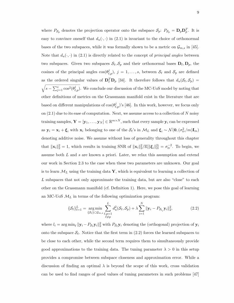
Remark 1. The MC-UoS model and the learning problem (2.2) can be further motivated
as follows. Consider a set of facial images of individuals under varying illumination
conditions in the Extended Yale B dataset [49], as in Figs. 2.1(a) and 2.1(b). It is
generally agreed that all images of an individual in this case can be regarded as lying
near a 9-dimensional subspace [50], which can be computed in a straightforward manner
using singular value decomposition (SVD). The subspace distance defined in (2.1) can be
used in this case to identify similar-looking individuals. Given noisy training images of
such “similar” individuals, traditional methods for UoS learning such as sparse subspace
clustering (SSC) [13] that rely only on the approximation error will be prone to errors.
Fig. 2.1 provides a numerical validation of this claim, where it is shown that SSC has
good performance on noisy images of different-looking individuals (cf. Fig. 2.1(b)), but
its performance degrades in the case of similar-looking individuals (cf. Fig. 2.1(a)). The
MC-UoS learning problem (2.2), on the other hand, should be able to handle both cases
reliably because of the first term in (2.2) that penalizes subspaces that do not cluster on
the Grassmann manifold. We refer the reader to Section 2.5.3 for detailed experiments
that numerically validate this claim.
In this work, we study two variants of the MC-UoS learning problem described by
(2.2). In the first variant, all m dimensions of each training sample in Y are observed
and the geometry learning problem is exactly given by (2.2). In the second variant, it
is assumed that some of the m dimensions of each training sample in Y are unobserved
(i.e., missing), which then requires a recharacterization of (2.2) for the learning problem
to be well posed. We defer that recharacterization to Section 2.4. In order to quantify
the performance of our learning algorithms, we will resort to generation of noisy test
data as follows. Given noiseless (synthetic or real) data sample x with ‖x‖22 = 1, noisy
test sample z is given by z = x + ξ with the additive noise ξ ∼ N (0, (σ2te/m)Im).
11
(a) (b)
Figure 2.1: An example illustrating the limitations of existing methods for UoS learningfrom noisy training data. The top row in this figure shows examples of “clean” facialimages of four individuals in the Extended Yale B dataset [49], while the bottom rowshows noisy versions of these images, corresponding to σ2
tr = 0.1. The “ground truth”distance between the subspaces of the individuals in (a) is 1.7953, while it is 2.3664between the subspaces of the individuals in (b). State-of-the-art UoS learning methodshave trouble reliably learning the underlying subspaces whenever the subspaces areclose to each other. Indeed, while the distance between the two subspaces learned bythe SSC algorithm [13] from noisy images of the individuals in (b) is 2.4103, it is 2.4537for the case of “similar-looking” individuals in (a).
We will then report the metric of average approximation error of noisy test data using
the learned subspaces for synthetic and real data. Finally, in the case of synthetic
data drawn from an MC-UoS, we will also measure the performance of our algorithms
in terms of average normalized subspace distances between the learned and the true
subspaces. We defer a formal description of both these metrics to Section 2.5.1, which
describes in detail the setup of our experiments.
2.2 MC-UoS Learning Using Complete Data
In order to reduce the effects of noisy training data, we begin with a pre-processing step
that centers the data matrix Y.1 This involves defining the mean of the samples in Y
as y = 1N
∑Ni=1 yi and then subtracting this mean from Y to obtain the centered data
Y = [y1, . . . , yN ], where yi = yi − y, i = 1, . . . , N . Next, we focus on simplification
of the optimization problem (2.2). To this end, we first define an L × N indicator
1While such pre-processing is common in many geometry learning algorithms, it is not central toour framework.

12
matrix W that identifies memberships of the yi’s in different subspaces, where w`,i = 1,
` = 1, . . . , L, i = 1, . . . , N , if and only if yi is “closest” to subspace S`; otherwise,
w`,i = 0. Mathematically,
W =[w`,i ∈ 0, 1 : ∀i = 1, . . . , N,
L∑`=1
w`,i = 1]. (2.3)
Further, notice that ‖yi − PS`yi‖22 in (2.2) can be rewritten as
‖yi − PS`yi‖22 = ‖yi − PS` yi‖
22 = ‖yi‖22 − ‖DT
` yi‖22, (2.4)
where D` ∈ Rm×s denotes an (arbitrary) orthonormal basis of S`. Therefore, defining
D = [D1, . . . ,DL] to be a collection of orthonormal bases of S`’s, we can rewrite (2.2)
as (D,W) = arg minD,W F1(D,W) with the objective function F1(D,W) given by2
F1(D,W) =
L∑`,p=16=p
‖D` − PSpD`‖2F + λ
N∑i=1
L∑`=1
w`,i(‖yi‖22 − ‖DT` yi‖22). (2.5)
Minimizing (2.5) simultaneously over D and W is challenging and is likely to be
computationally infeasible. Instead, we adopt an alternate minimization approach [51,
52], which involves iteratively solving (2.5) by alternating between the following two
steps: (i) minimizing F1(D,W) over W for a fixed D, which we term as the subspace
assignment step; and (ii) minimizing F1(D,W) over D for a fixed W, which we term
as the subspace update stage. To begin this alternate minimization, we start with an
initial D in which each block D` ∈ Rm×s is a random orthonormal basis. Next, we
fix this D and carry out subspace assignment, which now amounts to solving for each
i = 1, . . . , N ,
li = arg min`=1,...,L
‖yi − PS` yi‖22 = arg max
`=1,...,L‖DT
` yi‖22, (2.6)
and then setting wli,i = 1 and w`,i = 0 ∀` 6= li. In order to move to the subspace
update step, we fix the matrix W and focus on optimizing F1(D,W) over D. However,
this step requires more attention since minimizing over the entire D at once will also
lead to a large-scale optimization problem. We address this problem by once again
2Note that the minimization here is being carried out under the assumption of D`’s being orthonor-mal and W being described by (2.3).
13
resorting to block-coordinate descent (BCD) [51] and updating only one D` at a time
while keeping the other Dp’s (p 6= `) fixed in (2.5). In this regard, suppose we are
in the process of updating D` for a fixed ` during the subspace update step. Define
c` = i ∈ 1, . . . , N : w`,i = 1 to be the set containing the indices of all yi’s that
are assigned to S` (equivalently, D`) and let Y` = [yi : i ∈ c`] be the corresponding
m×|c`| matrix. Then it can be shown after some manipulations of (2.5) that updating
D` is equivalent to solving the following problem:
D` = arg minQ∈Vm,s
∑p 6=`‖Q− PSpQ‖2F +
λ
2(‖Y`‖2F − ‖QT Y`‖2F )
= arg maxQ∈Vm,s
tr(QT (
∑p6=`
DpDTp +
λ
2Y`Y
T` )Q
), (2.7)
where Vm,s denotes the Stiefel manifold, defined as the collection of allm×s orthonormal
matrices. Note that (2.7) has an intuitive interpretation. When λ = 0, (2.7) reduces to
the problem of finding a subspace that is closest to the remaining L−1 subspaces in our
collection. When λ =∞, (2.7) reduces to the PCA problem, in which case the learning
problem (2.2) reduces to the subspace clustering problem studied in [53]. By selecting an
appropriate λ ∈ (0,∞) in (2.7), we straddle the two extremes of subspace closeness and
data approximation. In order to solve (2.7), we define an m×m symmetric matrix A` =∑p 6=` DpD
Tp + λ
2 Y`YT` . It then follows from [54] that (2.7) has a closed-form solution
that involves eigendecomposition of A`. Specifically, D` = arg max tr(DT` A`D`) is
given by the first s eigenvectors of A` associated with its s-largest eigenvalues.
This completes our description of the subspace update step. We can now combine
the subspace assignment and subspace update steps to fully describe our algorithm
for MC-UoS learning. This algorithm, which we term metric-constrained union-of-
subspaces learning (MiCUSaL), is given by Algorithm 1. In terms of the complexity
of this algorithm in each iteration, notice that the subspace assignment step requires
O(mLsN) operations. In addition, the total number of operations needed to compute
the A`’s in each iteration is O(m2(Ls + N)). Finally, each iteration also requires L
eigendecompositions of m × m matrices, each one of which has O(m3) complexity.
Therefore, the computational complexity of MiCUSaL in each iteration is given by
O(m3L+m2N +m2Ls+mLsN). We conclude this discussion by pointing out that we
14
Algorithm 1: Metric-Constrained Union-of-Subspaces Learning (MiCUSaL)
Input: Training data Y ∈ Rm×N , number of subspaces L, dimension ofsubspaces s, and parameter λ.
Initialize: Random orthonormal bases D` ∈ Rm×sL`=1.
1: y = 1N
∑Ni=1 yi, yi = yi − y, i = 1, . . . , N .
2: while stopping rule do3: for i = 1 to N (Subspace Assignment) do4: li = arg max` ‖DT
` yi‖2.5: wli,i = 1 and ∀` 6= li, w`,i = 0.6: end for7: for ` = 1 to L (Subspace Update) do8: c` = i ∈ 1, . . . , N : w`,i = 1.9: Y` = [yi : i ∈ c`].
10: A` =∑
p6=` DpDTp + λ
2 Y`YT` .
11: Eigendecomposition of A` = U`Σ`UT` .
12: D` = Columns of U` corresponding to the s-largest diagonal elements in Σ`.13: end for14: end while
Output: Orthonormal bases D` ∈ Rm×sL`=1.
cannot guarantee convergence of MiCUSaL to a global optimal solution. However, since
the objective function F1 in (2.5) is bounded below by zero and MiCUSaL ensures that
F1 does not increase after each iteration, it follows that MiCUSaL iterates do indeed
converge (possibly to one of the local optimal solutions). This local convergence, of
course, will be a function of the initialization of MiCUSaL. In this work, we advocate
the use of random subspaces for initialization, while we study the impact of such random
initialization in Section 2.5.
2.3 Practical Considerations
The MiCUSaL algorithm described in Section 2.2 requires knowledge of the number of
subspaces L and the dimension of subspaces s. In practice, however, one cannot assume
knowledge of these parameters a priori. Instead, one must estimate both the number
and the dimension of subspaces from the training data themselves. In this section,
we describe a generalization of the MiCUSaL algorithm that achieves this objective.
Our algorithm, which we term adaptive MC-UoS learning (aMiCUSaL), requires only
knowledge of loose upper bounds on L and s, which we denote by Lmax and smax,
15
respectively.
The aMiCUSaL algorithm initializes with a collection of random orthonormal bases
D = [D1, . . . ,DLmax ], where each basis D` is a point on the Stiefel manifold Vm,smax .
Similar to the case of MiCUSaL, it then carries out the subspace assignment and sub-
space update steps in an iterative fashion. Unlike MiCUSaL, however, we also greedily
remove redundant subspaces from our collection of subspaces S`Lmax`=1 after each sub-
space assignment step. This involves removal of D` from D if no signals in our training
data get assigned to the subspace S`. This step of greedy subspace pruning ensures that
only “active” subspaces survive before the subspace update step.
Once the aMiCUSaL algorithm finishes iterating between subspace assignment, sub-
space pruning, and subspace update, we move onto the step of greedy subspace merging,
which involves merging of pairs of subspaces that are so close to each other that even
a single subspace of the same dimension can be used to well approximate the data
represented by the two subspaces individually.3 In this step, we greedily merge pairs of
closest subspaces as long as their normalized subspace distance is below a predefined
threshold εmin ∈ [0, 1). Mathematically, the subspace merging step involves first finding
the pair of subspaces (S`∗ ,Sp∗) that satisfies
(`∗, p∗) = arg min` 6=p
du(S`,Sp) s.t.du(S`∗ ,Sp∗)√
smax≤ εmin. (2.8)
We then merge S`∗ and Sp∗ by setting c`∗ = c`∗ ∪ cp∗ and Y`∗ = [yi : i ∈ c`∗ ],
where c`∗ , cp∗ are as defined in Algorithm 1. By defining an m×m symmetric matrix
A`∗ =∑6=`∗,p∗ D`D
T` + λ
2 Y`∗YT`∗ , D`∗ is then set equal to the first smax eigenvectors of
A`∗ associated with its smax-largest eigenvalues. Finally, we remove Dp∗ from D. This
process of finding the closest pair of subspaces and merging them is repeated until the
normalized subspace distance between every pair of subspaces becomes greater than
εmin. We assume without loss of generality that L subspaces are left after this greedy
subspace merging, where each S` (` = 1, . . . , L) is a subspace in Rm of dimension smax.
After subspace merging, we move onto the step of estimation of the dimension, s,
3Note that the step of subspace merging is needed due to our lack of knowledge of the true numberof subspaces in the underlying model. In particular, the assumption here is that the merging thresholdεmin in Algorithm 2 satisfies εmin ε√
s.
16
Algorithm 2: Adaptive MC-UoS Learning (aMiCUSaL)
Input: Training data Y ∈ Rm×N , loose upper bounds Lmax and smax, andparameters λ, k1, k2, εmin.
Initialize: Random orthonormal bases D` ∈ Rm×smaxLmax`=1 , and set L = Lmax.
1: y = 1N
∑Ni=1 yi, yi = yi − y, i = 1, . . . , N .
2: while stopping rule do3: Fix D and update W using (2.6). Also, set T = ∅ and L1 = 0.4: for ` = 1 to L (Subspace Pruning) do5: c` = i ∈ 1, . . . , N : w`,i = 1.6: If |c`| 6= 0 then cL1+1 = c`, YL1+1 = [yi : i ∈ c`], L1 = L1 + 1 and T = T ∪ `.7: end for8: D = [DT(1) , . . . ,DT(L1)
] and L = L1.
9: Update each D` (` = 1, . . . , L) in D using (2.7).10: end while11: (`∗, p∗) = arg min 6=p,`,p=1,...,L
du(S`,Sp).
12: whiledu(S`∗ ,Sp∗ )√
smax≤ εmin (Subspace Merging) do
13: Merge S`∗ and Sp∗ , and update Y`∗ and D`∗ .
14: D = [D1, . . . ,D`∗ , . . . ,Dp∗−1,Dp∗+1, . . . ,DL] and L = L− 1.
15: (`∗, p∗) = arg min 6=p,`,p=1,...,Ldu(S`,Sp).
16: end while17: Fix D, update W ∈ RL×N using (2.6), and update c`L`=1.
18: for ` = 1 to L do19: Y` = [yi : i ∈ c`] and Y` = D`D
T` Y`.
20: Calculate s` using (2.9) and (2.10).21: end for22: s = maxs1, . . . , sL.23: D` = First s columns of D`, ` = 1, . . . , L.
24: Initialize Algorithm 1 with D`L`=1 and update D`L`=1 using Algorithm 1.
Output: Orthonormal bases D` ∈ Rm×sL`=1.
of the subspaces. To this end, we first estimate the dimension of each subspace S`,
denoted by s`, and then s is selected as the maximum of these s`’s. There have been
many efforts in the literature to estimate the dimension of a subspace; see, e.g., [55–58]
for an incomplete list. In this work, we focus on the method given in [55], which
formulates the maximum likelihood estimator (MLE) of s`. This is because: (i) the
noise level is unknown in our problem, and (ii) the MLE in [55] has a simple form.
However, the MLE of [55] is sensitive to noise. We therefore first apply a “smoothing”
process before using that estimator. This involves first updating W (i.e., c`’s) using the
updated D and “denoising” our data by projecting Y` onto S`, given by Y` = D`DT` Y`,

17
and then using Y` to estimate s`. For a given column y in Y` and a fixed number of
nearest neighbors k0, the unbiased MLE of s` with respect to y is given by [55]
sk0` (y) =[ 1
k0 − 2
k0−1∑a=1
logΓk0(y)
Γa(y)
]−1, (2.9)
where Γa(y) is the `2 distance between y and its a-th nearest neighbor in Y`. An
estimate of s` can now be written as the average of all estimates with respect to every
signal in Y`, i.e., sk0` = 1|c`|∑
i∈c`sk0` (yi). In fact, as suggested in [55], we estimate s`
by averaging over a range of k0 = k1, . . . , k2, i.e.,
s` =1
k2 − k1 + 1
k2∑k0=k1
sk0` . (2.10)
Once we get an estimate s = max` s`, we trim each orthonormal basis by keeping only
the first s columns of each (ordered) orthonormal basis D` in our collection, which is
denoted by D`.4 Given the bases D` ∈ Rm×sL`=1, we finally run MiCUSaL again
that is initialized using these D`’s until it converges. Combining all the steps men-
tioned above, we can now formally describe adaptive MC-UoS learning (aMiCUSaL) in
Algorithm 2.
2.4 MC-UoS Learning Using Missing Data
In this section, we study MC-UoS learning for the case of training data having missing
entries. To be specific, for each yi in Y, we assume to only observe its entries at locations
given by the set Ωi ⊂ 1, . . . ,m with |Ωi| > s, which is denoted by [yi]Ωi ∈ R|Ωi|.
Since we do not have access to the complete data, it is impossible to compute the
quantities ‖yi − PS`yi‖22 in (2.2) explicitly. But, it is shown in [59] that ‖[yi]Ωi −
PS`Ωi [yi]Ωi‖22 for uniformly random Ωi is very close to |Ωi|m ‖yi − PS`yi‖22 with very
high probability as long as |Ωi| is slightly greater than s. Here, PS`Ωi is defined as
PS`Ωi = [D`]Ωi,:([D`]Ωi,:)† with ([D`]Ωi,:)
† =([D`]
TΩi,:
[D`]Ωi,:
)−1[D`]
TΩi,:
. Motivated by
this, we replace ‖yi − PS`yi‖22 by m|Ωi|‖[yi]Ωi − PS`Ωi [yi]Ωi‖22 in (2.2) and reformulate
4Recall that the columns of D` correspond to the eigenvectors of A`. Here, we are assuming thatthe order of these eigenvectors within D` corresponds to the nonincreasing order of the eigenvalues ofA`. Therefore, D` comprises the eigenvectors of A` associated with its s-largest eigenvalues.
18
the MC-UoS learning problem as (D,W) = arg minD,W F2(D,W) with the objective
function F2(D,W) given by
F2(D,W) =
L∑`,p=16=p
‖D` − PSpD`‖2F + λ
N∑i=1
L∑`=1
w`,im
|Ωi|∥∥[yi]Ωi − PS`Ωi [yi]Ωi
∥∥2
2. (2.11)
As in Section 2.2, we propose to solve this problem by making use of alternating
minimization that comprises subspace assignment and subspace update steps. To this
end, we again initialize D such that each block D` ∈ Rm×s is a random orthonormal
basis. Next, when D is fixed, subspace assignment corresponds to solving for each
i = 1, . . . , N ,
li = arg min`=1,...,L
‖[yi]Ωi − PS`Ωi [yi]Ωi‖22, (2.12)
and then setting wli,i = 1 and w`,i = 0 ∀` 6= li. When W is fixed, we carry out subspace
update using BCD again, in which case minD F2(D,W) for a fixed W can be decoupled
into L distinct problems of the form D` = arg minD`∈Vm,s f2(D`), ` = 1, . . . , L, with
f2(D`) = −tr(DT` A`D`) +
λ
2
∑i∈c`
m
|Ωi|∥∥[yi]Ωi − PS`Ωi [yi]Ωi
∥∥2
2. (2.13)
Here, c` is as defined in Section 2.2 and A` =∑
p6=` DpDTp . It is also easy to ver-
ify that f2(D`) is invariant to the choice of the orthonormal basis of S`; hence, we
can treat minD`∈Vm,s f2(D`) as an optimization problem on the Grassmann mani-
fold [60]. Note that we can rewrite f2(D`) as f2(D`) =∑|c`|
q=0 f(q)2 (D`), where f
(0)2 (D`) =
−tr(DT` A`D`) and f
(q)2 (D`) = λm
2|Ωc`(q)|‖[yc`(q) ]Ωc`(q)
− PS`Ωc`(q)[yc`(q) ]Ωc`(q)
‖22 for q =
1, . . . , |c`|. In here, c`(q) denotes the q-th element in c`. In order to minimize f2(D`),
we employ incremental gradient descent procedure on Grassmann manifold [61], which
performs the update with respect to a single component of f2(D`) in each step. To be
specific, we first compute the gradient of a single cost function f(q)2 (D`) in f2(D`), and
move along a short geodesic curve in the gradient direction. For instance, the gradient
of f(0)2 (D`) is
∇f (0)2 = (Im −D`D
T` )df
(0)2
dD`= −2(Im −D`D
T` )A`D`. (2.14)
19
Then the geodesic equation emanating from D` in the direction −∇f (0)2 with a step
length η is given by [60]
D`(η) = D`V` cos(Σ`η)VT` + U` sin(Σ`η)VT
` , (2.15)
where U`Σ`VT` is the SVD decomposition of −∇f (0)
2 . The update of D` with respect
to f(q)2 (D`) (q = 1, . . . , |c`|) can be performed as in the GROUSE algorithm [62] but
with a step size λm2|Ωc`(q)
|η. In order for f2 to converge, we also reduce the step size after
each iteration [62]. We complete this discussion by presenting our learning algorithm for
missing data in Algorithm 3, termed robust MC-UoS learning (rMiCUSaL). By defining
T = maxi |Ωi|, the subspace assignment step of rMiCUSaL requires O(TLs2N) flops in
each iteration [62]. Computing the A`’s in each iteration requires O(m2Ls) operations.
Next, the cost of updating each D` with respect to f(0)2 (D`) is O(m3), while it is O(ms+
Ts2) with respect to f(q)2 (D`) for q 6= 0 [62]. It therefore follows that the computational
complexity of rMiCUSaL in each iteration is O(m3L + m2Ls + msN + TLs2N). We
refer the reader to Section 2.5 for exact running time of rMiCUSaL on training data.
2.5 Experimental Results
In this section, we examine the effectiveness of MC-UoS learning using Algorithms 1–
3. For the complete data experiments, we compare MiCUSaL/aMiCUSaL with sev-
eral state-of-the-art UoS learning algorithms such as Block-Sparse Dictionary Design
(SAC+BK-SVD) [30], K-subspace clustering (K-sub) [53], Sparse Subspace Clustering
(SSC) [13], Robust Sparse Subspace Clustering (RSSC) [34], Robust Subspace Clus-
tering via Thresholding (TSC) [33], as well as with Principal Component Analysis
(PCA) [1]. In the case of the UoS learning algorithms, we use codes provided by their
respective authors. In the case of SSC, we use the noisy variant of the optimization
program in [13] and set λz = αz/µz in all experiments, where λz and µz are as de-
fined in [13, (13) & (14)], while the parameter αz varies in different experiments. In
the case of RSSC, we set λ = 1/√s as per [34], while the tuning parameter in TSC
is set q = max(3, dN/(L × 20)e) when L is provided. For the case of training data
having missing entries, we compare the results of rMiCUSaL with k-GROUSE [22] and

20
Algorithm 3: Robust MC-UoS learning (rMiCUSaL)
Input: Training data [yi]ΩiNi=1, number of subspaces L, dimension ofsubspaces s, and parameters λ and η.
Initialize: Random orthonormal bases D` ∈ Rm×sL`=1.
1: while stopping rule do2: for i = 1 to N (Subspace Assignment) do3: li = arg min` ‖[yi]Ωi − PS`Ωi [yi]Ωi‖22.4: wli,i = 1 and ∀` 6= li, w`,i = 0.5: end for6: for ` = 1 to L (Subspace Update) do7: c` = i ∈ 1, . . . , N : w`,i = 1, t = 0.8: while stopping rule do9: t = t+ 1, ηt = η
t .10: A` =
∑p 6=` DpD
Tp , ∆` = 2(Im −D`D
T` )A`D`.
11: D` = D`V` cos(Σ`ηt)VT` + U` sin(Σ`ηt)V
T` , where U`Σ`V
T` is the compact
SVD of ∆`.12: for q = 1 to |c`| do13: θ = ([D`]Ωc`(q)
,:)†[yc`(q) ]Ωc`(q)
, ω = D`θ.
14: r = 0m, [r]Ωc`(q)= [yc`(q) ]Ωc`(q)
− [ω]Ωc`(q).
15: D` = D` +(
(cos(µ λm|Ωc`(q)
|ηt)− 1) ω‖ω‖2 + sin(µ λm
|Ωc`(q)|ηt)
r‖r‖2
)θT
‖θ‖2 , where
µ = ‖r‖2‖ω‖2.16: end for17: end while18: end for19: end while
Output: Orthonormal bases D` ∈ Rm×sL`=1.
GROUSE [62].5
In order to generate noisy training and test data in these experiments, we start
with sets of “clean” training and test samples, denoted by X and Xte, respectively.
We then add white Gaussian noise to these samples to generate noisy training and
test samples Y and Z, respectively. In the following, we use σ2tr and σ2
te to denote
variance of noise added to training and test samples, respectively. In the missing data
experiments, for every fixed noise variance σ2tr, we create training (but not test) data
with different percentages of missing values, where the number of missing entries is
set to be 10%, 30% and 50% of the signal dimension. Our reported results are based
5As discussed in [63], we omit the results for SSC with missing data in this thesis because it fillsin the missing entries with random values, resulting in relatively poor performance for problems withmissing data.
21
on random initializations of MiCUSaL and aMiCUSaL algorithms. In this regard, we
adopt the following simple approach to mitigate any stability issues that might arise due
to random initializations. We perform multiple random initializations for every fixed
Y and λ, and then retain the learned MC-UoS structure that results in the smallest
value of the objective function in (2.2). We also use a similar approach for selecting the
final structures returned by K-subspace clustering and Block-Sparse Dictionary Design,
with the only difference being that (2.2) in this case is replaced by the approximation
error of training data.
2.5.1 Experiments on Synthetic Data
In the first set of synthetic experiments, we consider L = 5 subspaces of the same
dimension s = 13 in an m = 180-dimensional ambient space. The five subspaces S`’s of
R180 are defined by their orthonormal bases T` ∈ Rm×s5`=1 as follows. We start with
a random orthonormal basis T1 ∈ Rm×s and for every ` ≥ 2, we set T` = orth(T`−1 +
tsW`) where every entry in W` ∈ Rm×s is a uniformly distributed random number
between 0 and 1, and orth(·) denotes the orthogonalization process. The parameter ts
controls the distance between subspaces, and we set ts = 0.04 in these experiments.
After generating the subspaces, we generate a set of n` points from S` as X` = T`C`,
where C` ∈ Rs×n` is a matrix whose elements are drawn independently and identically
from N (0, 1) distribution. In here, we set n1 = n3 = n5 = 150, and n2 = n4 = 100;
hence, N = 650. We then stack all the data into a matrix X = [X1, . . . ,X5] = xiNi=1
and normalize all the samples to unit `2 norms. Test data Xte ∈ Rm×N are produced
using the same foregoing strategy. Then we add white Gaussian noise with different
expected noise power to both X and Xte. Specifically, we set σ2tr to be 0.1, while σ2
te
ranges from 0.1 to 0.5. We generate X and Xte 10 times, while Monte Carlo simulations
for noisy data are repeated 20 times for every fixed X and Xte. Therefore, the results
reported in here correspond to an average of 200 random trials.
We make use of the collection of noisy samples, Y, to learn a union of L subspaces
of dimension s and stack the learned orthonormal bases D`L`=1 into D. In this set

22
Table 2.1: davg of different UoS learning algorithms for synthetic data
davg Algorithms
Complete
MiCUSaL(λ = 2) SAC+BK-SVD K-sub0.1331 0.2187 0.1612
SSC RSSC TSC0.1386 0.2215 0.2275
Missing
rMiCUSaL-10% rMiCUSaL-30% rMiCUSaL-50%0.1661 0.1788 0.2047
k-GROUSE-10% k-GROUSE-30% k-GROUSE-50%0.3836 0.4168 0.4649
0.1 0.2 0.3 0.4 0.50.02
0.04
0.06
0.08
test noise level (σte
2)
rela
tive e
rror
MiCUSaLSAC+BK−SVDK−sub
SSC
RSSC
TSC
PCA
(a)
0.1 0.2 0.3 0.4 0.50.02
0.03
0.04
0.05
0.06
test noise level (σte
2)
rela
tive e
rror
MiCUSaL−λ=1
MiCUSaL−λ=2
MiCUSaL−λ=4
MiCUSaL−λ=8
MiCUSaL−λ=20
K−sub
(b)
0.1 0.2 0.3 0.4 0.50.024
0.044
0.064
0.084
test noise level (σte
2)
rela
tive
err
or
10%
30%
50%
k-GROUSE
rMiCUSaL
GROUSE
(c)
0.1 0.2 0.3 0.4 0.50.022
0.032
0.042
0.052
0.062
test noise level (σte
2)
rela
tive e
rror
rMiCUSaL−λ=1
rMiCUSaL−λ=2
rMiCUSaL−λ=4
rMiCUSaL−λ=10
rMiCUSaL−λ=20
k−GROUSE
(d)
Figure 2.2: Comparison of MC-UoS learning performance on synthetic data. (a) and(c) show relative errors of test signals for complete and missing data experiments, whereλ = 2 for both MiCUSaL and rMiCUSaL. The numbers in the legend of (c) indicatethe percentages of missing entries within the training data. (b) and (d) show relativeerrors of test signals for MiCUSaL and rMiCUSaL (with 10% missing entries) usingdifferent λ’s.

23
of experiments, we use MiCUSaL and rMiCUSaL for complete and missing data ex-
periments, respectively. The number of random initializations used to select the final
geometric structure in these experiments is 8 for every fixed Y and λ. We use the fol-
lowing metrics for performance analysis of MC-UoS learning. Since we have knowledge
of the ground truth S`’s, represented by their ground truth orthonormal bases T`’s, we
first find the pairs of estimated and true subspaces that are the best match, i.e., D`
is matched to T using = arg maxp ‖DT` Tp‖F . We also ensure that no two D`’s are
matched to the same T. Then we define davg to be the average normalized subspace
distances between these pairs, i.e., davg = 1L
∑L`=1
√s−tr(DT
` TTT D`)
s . A smaller davg
indicates better performance of MC-UoS learning. Also, if the learned subspaces are
close to the ground truth, they are expected to have good representation performance
on test data. A good measure in this regard is the mean of relative reconstruction
errors of the test samples using learned subspaces. To be specific, if the training data
are complete, we first represent every test signal z such that z ≈ Dταte + y where
τ = arg max` ‖DT` (z − y)‖22 (recall that y = 1
N
∑Ni=1 yi) and αte = DT
τ (z − y). The
relative reconstruction error with respect to its noiseless part, x, is then defined as
‖x−(Dταte+y)‖22‖x‖22
. On the other hand, if the training data have missing entries then
for a test signal z, the reconstruction error with respect to x is simply calculated by
‖x−DτDTτ z‖22
‖x‖22, where τ = arg max` ‖DT
` z‖22.
To compare with other UoS learning methods, we choose λ = 2 for both MiCUSaL
and rMiCUSaL. In the complete data experiments, we perform SSC with αz = 60. We
set the subspace dimension for PCA to be the (unrealizable, ideal) one that yields the
best denoising result on training samples. We also use the same subspace dimension
(again, unrealizable and ideal) for GROUSE in the corresponding missing data exper-
iments. Table 2.1 summarizes the davg’s of different UoS learning algorithms for both
complete and missing data experiments. As can be seen, MiCUSaL produces smaller
davg’s, which in turn leads to smaller relative errors of test data; see Fig. 2.2(a) for
a validation of this claim. For MC-UoS learning with missing data, rMiCUSaL also
learns a better MC-UoS in that: (i) for a fixed percentage of the number of missing
observations in the training data, the davg for rMiCUSaL is much smaller than the

24
one for k-GROUSE (see Table 2.1); and (ii) rMiCUSaL outperforms k-GROUSE and
GROUSE in terms of smaller reconstruction errors of test data. Moreover, we can infer
from Fig. 2.2(c) that for a fixed σte, when the number of missing entries increases, the
performance of rMiCUSaL degrades less compared to k-GROUSE. We also test the
UoS learning performance with complete data when the subspaces are not close to each
other (e.g., ts = 0.2). In this case, all the UoS learning algorithms, including MiCUSaL,
learn the subspaces successfully. We omit these plots because of space constraints.
Table 2.2: davg of MiCUSaL and rMiCUSaL for different λ’s using synthetic data
davg λ
MiCUSaLλ = 1 λ = 2 λ = 4 λ = 8 λ = 200.1552 0.1331 0.1321 0.1378 0.1493
rMiCUSaL λ = 1 λ = 2 λ = 4 λ = 10 λ = 20(10% missing) 0.2096 0.1661 0.1725 0.2065 0.2591
For both MiCUSaL and rMiCUSaL, we also analyze the effect of the key parameter,
λ, on the UoS learning performance. We implement MiCUSaL with λ ∈ 1, 2, 4, 8, 20
in the complete data experiments and select λ ∈ 1, 2, 4, 10, 20 for rMiCUSaL in the
missing data experiments, where the number of missing entries in the training data
is 10% of the signal dimension. The results are shown in Fig. 2.2(b), Fig. 2.2(d) and
Table 2.2. We can see when λ = 1, both the davg’s and reconstruction errors of the
test data are large for MiCUSaL and rMiCUSaL. This is because the learned subspaces
are too close to each other, which results in poor data representation capability of the
learned D`’s. When λ = 2 or 4, both these algorithms achieve good performance in
terms of small davg’s and relative errors of test data. As λ increases further, both davg
and relative errors of test data also increase. Furthermore, as λ grows, the curves of
relative errors of test data for MiCUSaL and rMiCUSaL get closer to the ones for K-
sub and k-GROUSE, respectively. This phenomenon coincides with our discussion in
Section 2.2 and 2.4. Finally, we note that both MiCUSaL and rMiCUSaL achieve their
best performance when λ ∈ [2, 4], and deviations of the representation errors of test
data are very small when λ falls in this range.
Next, we study the effect of random initialization of subspaces on MiCUSaL perfor-
mance by calculating the standard deviation of the mean of the reconstruction errors
25
of the test data for the 8 random initializations. The mean of these 200 standard devi-
ations ends up being only 0.003 for all σte’s when λ = 2. In addition, as λ gets larger,
the variation of the results increases only slightly (the mean of the standard deviations
is 0.0034 for λ = 8). On the other hand, the mean of the standard deviations for
K-sub is 0.0039. Furthermore, the performance gaps between MiCUSaL and all other
methods are larger than 0.003. Finally, the learned MC-UoS structure that results in
the smallest value of the objective function (2.2) always results in the best denoising
performance. This suggests that MiCUSaL always generates the best results and it is
mostly insensitive to the choice of initial subspaces during the random initialization.
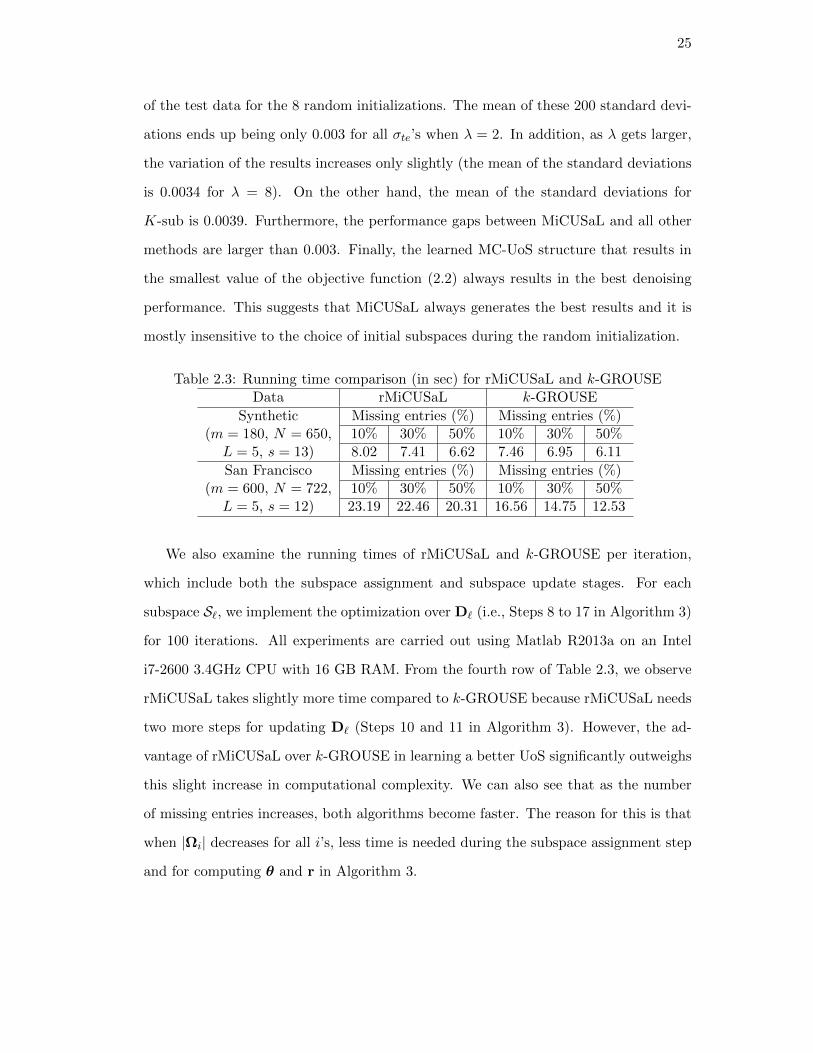
Table 2.3: Running time comparison (in sec) for rMiCUSaL and k-GROUSEData rMiCUSaL k-GROUSE
Synthetic Missing entries (%) Missing entries (%)(m = 180, N = 650, 10% 30% 50% 10% 30% 50%L = 5, s = 13) 8.02 7.41 6.62 7.46 6.95 6.11
San Francisco Missing entries (%) Missing entries (%)(m = 600, N = 722, 10% 30% 50% 10% 30% 50%L = 5, s = 12) 23.19 22.46 20.31 16.56 14.75 12.53
We also examine the running times of rMiCUSaL and k-GROUSE per iteration,
which include both the subspace assignment and subspace update stages. For each
subspace S`, we implement the optimization over D` (i.e., Steps 8 to 17 in Algorithm 3)
for 100 iterations. All experiments are carried out using Matlab R2013a on an Intel
i7-2600 3.4GHz CPU with 16 GB RAM. From the fourth row of Table 2.3, we observe
rMiCUSaL takes slightly more time compared to k-GROUSE because rMiCUSaL needs
two more steps for updating D` (Steps 10 and 11 in Algorithm 3). However, the ad-
vantage of rMiCUSaL over k-GROUSE in learning a better UoS significantly outweighs
this slight increase in computational complexity. We can also see that as the number
of missing entries increases, both algorithms become faster. The reason for this is that
when |Ωi| decreases for all i’s, less time is needed during the subspace assignment step
and for computing θ and r in Algorithm 3.

26
(a) (b)
Figure 2.3: (a) San Francisco City Hall image. (b) Paris City Hall image.
2.5.2 Experiments on City Scene Data
To further show the effectiveness of the proposed approaches, we test our proposed
methods on real-world city scene data. First, we study the performance of our methods
on San Francisco City Hall image, as shown in Fig. 2.3(a). To generate the clean
training and test data, we split the image into left and right subimages of equal size.
Then we extract all 30× 20 nonoverlapping image patches from the left subimage and
reshape them into N = 722 column vectors of dimension m = 600. All these vectors
are normalized to have unit `2 norms and are then used as signals in X. Test signals in
Xte ∈ R600×722 are extracted in the same way from the right subimage. White Gaussian
noise is then added to X and Xte separately, forming Y and Z, respectively. In these
experiments, σ2tr is set to be 0.02 and 0.05, while σ2
te again ranges from 0.1 to 0.5. The
Monte Carlo simulations for noisy data are repeated 50 times and the results reported
here correspond to the average of these 50 trials. Note that each patch is treated as
a single signal here, and our goal is to learn an MC-UoS from Y such that every test
patch can be reliably denoised using the learned subspaces.
We perform aMiCUSaL on the training data Y with parameters Lmax = 8, smax =
20, λ = 4, k1 = 6, k2 = 10 and εmin = 0.08. The number of random initializations
that are used to arrive at the final MC-UoS structure using aMiCUSaL is 10 for every
fixed Y. The output L from aMiCUSaL is 4 or 5 and s is always between 11 and 13.
We also perform MiCUSaL with the same L and s 10 times. For fair comparison, we
also use the method in this thesis to get the dimension of the subspace for PCA, in
27
0.1 0.2 0.3 0.4 0.50.05
0.055
0.06
0.065
test noise level (σte
2)
rela
tive
err
or
MiCUSaLaMiCUSaLSAC+BK−SVDK−sub
SSC
RSSC
TSC
PCA
(a) σ2tr = 0.02
0.1 0.2 0.3 0.4 0.50.05
0.055
0.06
0.065
0.07
test noise level (σte
2)
rela
tive
err
or
10%
30%
50%
k-GROUSE
rMiCUSaL
GROUSE
(b) σ2tr = 0.02
0.1 0.2 0.3 0.4 0.50.05
0.055
0.06
0.065
test noise level (σte
2)
rela
tive
err
or
rMiCUSaL−λ=2
rMiCUSaL−λ=4
rMiCUSaL−λ=6
rMiCUSaL−λ=10
rMiCUSaL−λ=20
k−GROUSE
(c) σ2tr = 0.02
0.1 0.2 0.3 0.4 0.50.051
0.056
0.061
0.066
test noise level (σte
2)
rela
tive
err
or
MiCUSaLaMiCUSaLSAC+BK−SVDK−sub
SSC
RSSC
TSC
PCA
(d) σ2tr = 0.05
0.1 0.2 0.3 0.4 0.50.052
0.057
0.062
0.067
0.072
test noise level (σte
2)
rela
tive
err
or
10%
30%
50%
k-GROUSE
rMiCUSaL
GROUSE
(e) σ2tr = 0.05
0.1 0.2 0.3 0.4 0.50.05
0.055
0.06
0.065
test noise level (σte
2)
rela
tive
err
or
rMiCUSaL−λ=2
rMiCUSaL−λ=4
rMiCUSaL−λ=6
rMiCUSaL−λ=10
rMiCUSaL−λ=20
k−GROUSE
(f) σ2tr = 0.05
Figure 2.4: Comparison of MC-UoS learning performance on San Francisco City Halldata. (a) and (d) show relative errors of test signals for complete data experiments. (b)and (e) show relative errors of test signals for missing data experiments. The numbers inthe legend of (b) and (e) indicate the percentages of missing entries within the trainingdata. (c) and (f) show relative errors of test signals for rMiCUSaL (with 10% missingentries) using different λ’s.
which case the estimated s is always 10. Note that for all state-of-the-art UoS learning
algorithms, we use the same L and s as aMiCUSaL instead of using the L generated by
the algorithms themselves. The reason for this is as follows. The returned L by SSC
(with αz = 40) is 1. Therefore SSC reduces to PCA in this setting. The output L for
RSSC is also 4 or 5, which coincides with our algorithm. The estimation of L (with
q = 2 max(3, dN/(L × 20)e)) for TSC is sensitive to the noise and data. Specifically,
the estimated L is always from 6 to 9 for σ2tr = 0.02 and L is always 1 when σ2
tr = 0.05,
which results in poorer performance compared to the case when L = 4 or 5 for both
training noise levels. In the missing data experiments, we set L = 5 and s = 12 for
rMiCUSaL (with λ = 4) and k-GROUSE, and s = 10 for GROUSE. Fig. 2.4(a) and
Fig. 2.4(d) describe the relative reconstruction errors of test samples when the training
data are complete. We see both MiCUSaL and aMiCUSaL learn a better MC-UoS
since they give rise to smaller relative errors of test data. Further, the average standard
deviation of the mean of relative errors for test data is around 0.00015 for MiCUSaL and
28
0.00045 for K-sub. It can be inferred from Fig. 2.4(b) and Fig. 2.4(e) that rMiCUSaL
also yields better data representation performance for the missing data case.
To examine the effect of λ on the denoising result in both complete and missing data
experiments, we first run aMiCUSaL with λ ∈ 1, 2, 4, 6, 8, 10 without changing other
parameters. When λ = 1 or 2, aMiCUSaL always returns L = 2 or 3 subspaces, but
the reconstruction errors of the test data are slightly larger than those for λ = 4. When
λ ≥ 6, the distances between the learned subspaces become larger, and the resulting
L will be at least 6 when εmin is fixed. However, the relative errors of test data are
still very close to the ones for λ = 4. This suggests that λ = 4 is a good choice in this
setting since it leads to the smallest number of subspaces L and the best representation
performance. We also perform rMiCUSaL with λ ∈ 2, 4, 6, 10, 20 while keeping L
and s fixed, where the number of missing entries in the training data is again 10%
of the signal dimension. We show the relative errors of test data in Fig. 2.4(c) and
Fig. 2.4(f). Similar to the results of the experiments with synthetic data, we again
observe the fact that when λ is small (e.g., λ = 2), the reconstruction errors of the test
data are large because the subspace closeness metric dominates in learning the UoS.
The results for λ = 4 and 6 are very similar. As λ increases further, the performance
of rMiCUSaL gets closer to that of k-GROUSE. We again report the running time
of rMiCUSaL and k-GROUSE per iteration in the seventh row of Table 2.3, where
we perform the optimization over each D` for 100 iterations in each subspace update
step for both rMiCUSaL and k-GROUSE. In these experiments, rMiCUSaL appears
much slower than k-GROUSE. However, as presented in Fig. 2.4(b) and Fig. 2.4(e), the
performance of rMiCUSaL is significantly better than k-GROUSE.
Next, we repeat these experiments for the complete data experiments using Paris
City Hall image in Fig. 2.3(b), forming X,Xte ∈ R600×950. We perform aMiCUSaL
using the same parameters (λ = 4) as in the previous experiments. The estimated L in
this case is always between 5 and 6 and s is always between 11 and 12. The estimated
dimension of the subspace in PCA is 9 or 10 when σ2tr = 0.02 and it is always 10 when
σ2tr = 0.05. In these experiments, we again use the same L and s as aMiCUSaL for all
state-of-the-art UoS learning algorithms. This is because the returned L by SSC (with

29
0.1 0.2 0.3 0.4 0.50.062
0.067
0.072
0.077
test noise level (σte
2)
rela
tive e
rror
MiCUSaLaMiCUSaLSAC+BK−SVDK−sub
SSC
RSSC
TSC
PCA
(a) σ2tr = 0.02
0.1 0.2 0.3 0.4 0.50.064
0.069
0.074
0.079
test noise level (σte
2)
rela
tive e
rror
MiCUSaLaMiCUSaLSAC+BK−SVDK−sub
SSC
RSSC
TSC
PCA
(b) σ2tr = 0.05
Figure 2.5: Comparison of MC-UoS learning performance on Paris City Hall data whenthe training data are complete.
αz = 20) is again 1 in this case. The estimated L by RSSC is usually 7 or 8, and the
reconstruction errors of test data are very close to the ones reported here. If we apply
TSC using the L estimated by itself (again, with q = 2 max(3, dN/(L× 20)e)), we will
have L = 4 when σ2tr = 0.02, while the relative errors of test data are very close to
the results shown here. For σ2tr = 0.05, TSC will again result in only one subspace.
The relative reconstruction errors of test data with different training noise levels are
shown in Fig. 2.5, from which we make the conclusion that our methods obtain small
errors, thereby outperforming all other algorithms. The average standard deviation of
the mean of relative errors for test data is also smaller for MiCUSaL (around 0.00023)
compared to K-sub (around 0.00037).
2.5.3 Experiments on Face Dataset
In this section, we work with the Extended Yale B dataset [49], which contains a set
of 192 × 168 cropped images of 38 subjects. For each individual, there are 64 images
taken under varying illumination conditions. We downsample the images to 48 × 42
pixels and each image is vectorized and treated as a signal; thus, m = 2016. It has been
shown in [50] that the set of images of a given subject taken under varying illumination
conditions can be well represented by a 9-dimensional subspace.
We first focus on a collection of images of subjects 5, 6 and 8 and normalize all the
images to have unit `2 norms. Some representative images are presented in the first row
of Fig. 2.6(a). Here we assume the images of these three subjects lie close to an MC-UoS
30
(a)
0.2 0.3 0.4 0.50.102
0.107
0.112
0.117
test noise level (σte
2)
rela
tive e
rror
MiCUSaLSAC+BK−SVDK−sub
SSC
RSSC
TSC
PCA
(b)
0.2 0.3 0.4 0.50.085
0.09
0.095
0.1
test noise level (σte
2)
rela
tive e
rror
MiCUSaLSAC+BK−SVDK−sub
SSC
RSSC
TSC
PCA
(c)
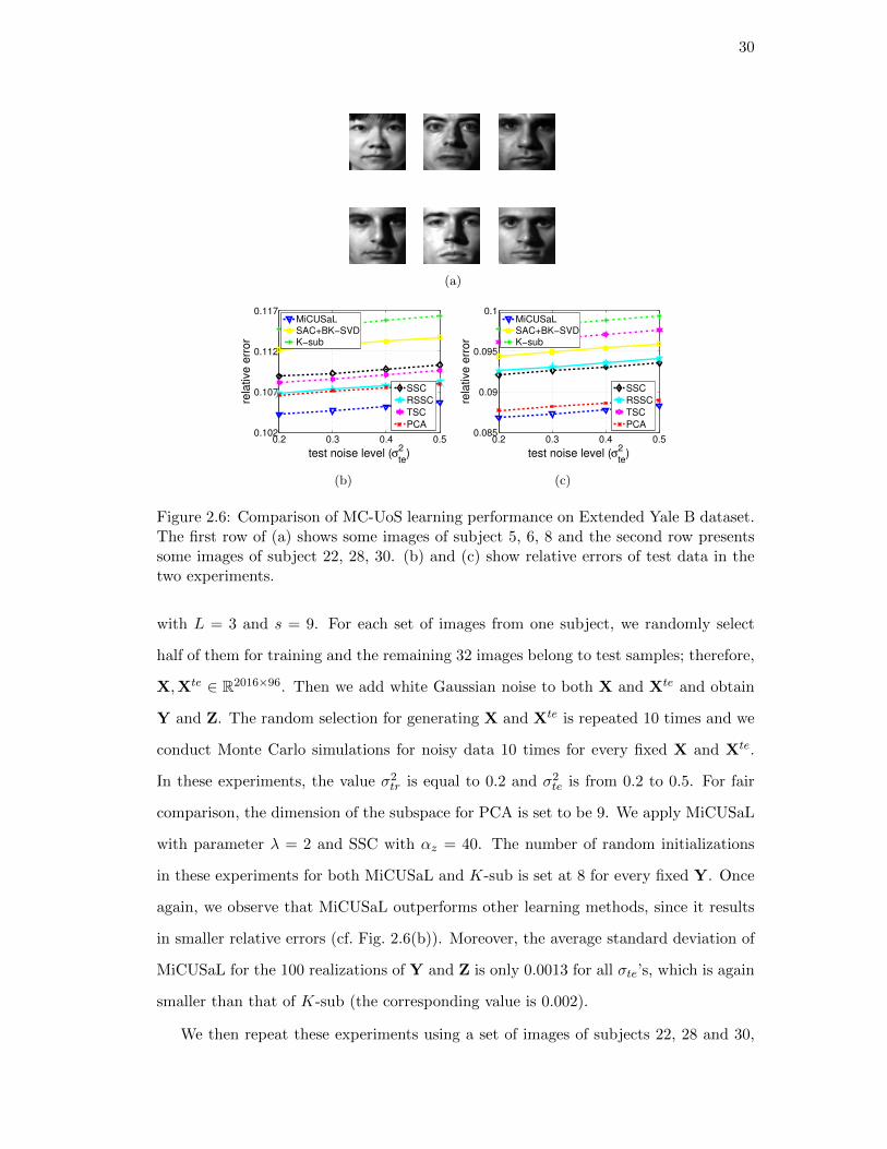
Figure 2.6: Comparison of MC-UoS learning performance on Extended Yale B dataset.The first row of (a) shows some images of subject 5, 6, 8 and the second row presentssome images of subject 22, 28, 30. (b) and (c) show relative errors of test data in thetwo experiments.
with L = 3 and s = 9. For each set of images from one subject, we randomly select
half of them for training and the remaining 32 images belong to test samples; therefore,
X,Xte ∈ R2016×96. Then we add white Gaussian noise to both X and Xte and obtain
Y and Z. The random selection for generating X and Xte is repeated 10 times and we
conduct Monte Carlo simulations for noisy data 10 times for every fixed X and Xte.
In these experiments, the value σ2tr is equal to 0.2 and σ2
te is from 0.2 to 0.5. For fair
comparison, the dimension of the subspace for PCA is set to be 9. We apply MiCUSaL
with parameter λ = 2 and SSC with αz = 40. The number of random initializations
in these experiments for both MiCUSaL and K-sub is set at 8 for every fixed Y. Once
again, we observe that MiCUSaL outperforms other learning methods, since it results
in smaller relative errors (cf. Fig. 2.6(b)). Moreover, the average standard deviation of
MiCUSaL for the 100 realizations of Y and Z is only 0.0013 for all σte’s, which is again
smaller than that of K-sub (the corresponding value is 0.002).
We then repeat these experiments using a set of images of subjects 22, 28 and 30,

31
and show some image samples in the second row of Fig. 2.6(a). We set L = 3, s = 9 and
λ = 2 for MiCUSaL and αz = 40 for SSC. We again provide evidence in Fig. 2.6(c) that
MiCUSaL yields better data representation performance in this setting. The average
standard deviation of the mean of the reconstruction errors for test data is around
0.0012 for MiCUSaL and 0.0019 for K-sub in this case.
32
Chapter 3
Metric-Constrained Kernel Union-of-Subspaces
3.1 Problem Formulation
In this chapter, we study the geometry learning problem corresponds to the case of
high-dimensional data drawn from a mixture of nonlinear manifolds in the ambient
space Rm. The basic premise in this case is that when data drawn from a mixture of
nonlinear manifolds are mapped through a nonlinear map φ : Rm → F to a higher-
dimensional feature space F ⊂ Rm with m≫ m, then the φ-mapped “images” of these
data can be modeled as lying near an MC-UoS ML in the feature space. In order to
learn this model, we once again assume access to a collection of N training samples,
Y = [y1, . . . ,yN ] ∈ Rm×N , with the fundamental difference here being that the mapped
training data φ(Y) = [φ(y1), . . . , φ(yN )] are now assumed to be drawn from an MC-
UoS ML =⋃L`=1 S` ⊂ Gm,s ⊂ F . Here, we also make the simplified assumption that
rank(φ(Y)) = N , which is justified as long as m≫ N and no two training samples are
identical. Our goal in this setting is to learn the (feature space) MC-UoSML using the
training data Y, which in theory can still be achieved by solving the following variant
of (2.2):
S`L`=1 = arg minS`⊂Gm,s
L∑`,p=1`6=p
d2u(S`,Sp) + λ
N∑i=1
‖φ(yi)− PSliφ(yi)‖22, (3.1)
where li = arg min` ‖φ(yi) − PS`φ(yi)‖22 with PS`φ(yi) denoting the (orthogonal) pro-
jection of φ(yi) onto the s-dimensional subspace S` in Rm.
In practice, however, solving (3.1) directly is likely to be computationally intractable
due to the extremely high dimensionality of the feature space. Instead, we are interested
in solving the problem of MC-UoS learning in the feature space using the “kernel
33
trick” [15], which involves transforming (3.1) into a learning problem that only requires
evaluations of inner products in F . Such a transformation can then be followed with
the use of a Mercer kernel κ, which is a positive semidefinite function κ : Rm×Rm → R
that satisfies κ(y,y′) = 〈φ(y), φ(y′)〉 for all y,y′ ∈ Rm, to develop algorithms that can
learn an MC-UoS in the feature space without explicit mapping of the training data
to the feature space. We term the learning of an MC-UoS in the feature space using
the kernel trick as metric-constrained kernel union-of-subspaces (MC-KUoS) learning.
Similar to the case of MC-UoS learning, we consider two scenarios in this work for
MC-KUoS learning. The first one of these scenarios corresponds to the standard setup
in which all m dimensions of each training sample in Y are observed, while the second
scenario corresponds to the case of “missing data” in which some dimensions of each
training sample in Y remain unobserved. Finally, we will evaluate the proposed MC-
KUoS learning algorithms using (i) the metric of average approximation error of noisy
test data, and (ii) their clustering performance on training data having either complete
or missing entries. We conclude here by pointing out that MC-KUoS learning invariably
also leads us to the problem of finding the “pre-images” of data in the feature space
induced by our chosen kernel (e.g., Gaussian or polynomial kernel) [6, 64], which will
also be addressed in this chapter.
Remark 2. It is worth noting here that (3.1) requires knowledge of the nonlinear map
φ. However, since we rely on the kernel trick for our MC-KUoS learning framework, we
only need access to an appropriate kernel κ. It is assumed in this chapter that such a
kernel is readily available to us. While learning the “best” kernel from training data is
an interesting extension of our work, it is beyond the scope of this thesis.
In the following sections, we present algorithms to solve the problem of MC-KUoS
learning from Y ∈ Rm×N for highly nonlinear data. We first generalize the MiCUSaL
algorithm using the kernel trick [15] to learn an MC-KUoS from complete data. To
deal with the case of “missing data,” we propose “kernel function value estimators” to
solve (3.1). Finally, we discuss the problem of finding the “pre-images” of data in the
feature space based on the MC-KUoS model in Section 3.4.
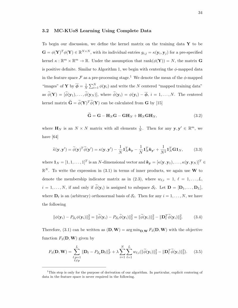
34
3.2 MC-KUoS Learning Using Complete Data
To begin our discussion, we define the kernel matrix on the training data Y to be
G = φ(Y)Tφ(Y) ∈ RN×N , with its individual entries gi,j = κ(yi,yj) for a pre-specified
kernel κ : Rm × Rm → R. Under the assumption that rank(φ(Y)) = N , the matrix G
is positive definite. Similar to Algorithm 1, we begin with centering the φ-mapped data
in the feature space F as a pre-processing stage.1 We denote the mean of the φ-mapped
“images” of Y by φ = 1N
∑Ni=1 φ(yi) and write the N centered “mapped training data”
as φ(Y) = [φ(y1), . . . , φ(yN )], where φ(yi) = φ(yi) − φ, i = 1, . . . , N . The centered
kernel matrix G = φ(Y)T φ(Y) can be calculated from G by [15]
G = G−HNG−GHN + HNGHN , (3.2)
where HN is an N × N matrix with all elements 1N . Then for any y,y′ ∈ Rm, we
have [64]
κ(y,y′) = φ(y)T φ(y′) = κ(y,y′)− 1
N1TNky −
1
N1TNky′ +
1
N21TNG1N , (3.3)
where 1N = [1, 1, . . . , 1]T is anN -dimensional vector and ky = [κ(y,y1), . . . , κ(y,yN )]T ∈
RN . To write the expression in (3.1) in terms of inner products, we again use W to
denote the membership indicator matrix as in (2.3), where w`,i = 1, ` = 1, . . . , L,
i = 1, . . . , N , if and only if φ(yi) is assigned to subspace S`. Let D = [D1, . . . ,DL],
where D` is an (arbitrary) orthonormal basis of S`. Then for any i = 1, . . . , N , we have
the following
‖φ(yi)− PS`φ(yi)‖22 = ‖φ(yi)− PS` φ(yi)‖22 = ‖φ(yi)‖22 − ‖DT` φ(yi)‖22. (3.4)
Therefore, (3.1) can be written as (D,W) = arg minD,W F3(D,W) with the objective
function F3(D,W) given by
F3(D,W) =
L∑`,p=1` 6=p
‖D` − PSpD`‖2F + λ
N∑i=1
L∑`=1
w`,i(‖φ(yi)‖22 − ‖DT` φ(yi)‖22). (3.5)
1This step is only for the purpose of derivation of our algorithm. In particular, explicit centering ofdata in the feature space is never required in the following.

35
Before discussing our algorithm to minimize (3.5) using the kernel trick, we further
simplify the terms in (3.5). We again define c` = i ∈ 1, . . . , N : w`,i = 1 to
be the set containing the indices of all φ(yi)’s that are assigned to S`, and let Y` =
[yi : i ∈ c`] be the corresponding m × |c`| matrix. Then the centered data that are
assigned to subspace S` can be denoted by φ(Y`) = [φ(yi) : i ∈ c`]. Since S` is
spanned by the columns of φ(Y`), we can write D` = φ(Y`)E`, where E` ∈ RN`×s
is some basis representation matrix with N` = |c`| such that D` is an orthonormal
matrix. Also, it is easy to verify that E` has to satisfy ET` [G]c`,c`E` = Is, where
[G]c`,c` = φ(Y`)T φ(Y`) denotes the centered kernel matrix for subspace S`. Now
instead of using D` explicitly for computations, it suffices to use c` and E` for MC-
KUoS learning and all the computations involving D` can be carried out using c`, E`
and the kernel trick. Specifically, notice that for any i = 1, . . . , N , we can write
‖φ(yi)‖22 − ‖DT` φ(yi)‖22 = κ(yi,yi)− ‖ET
` φ(Y`)T φ(yi)‖22, (3.6)
where κ(yi,yi) = κ(yi,yi)− 2N 1TNkyi+
1N2 1TNG1N . To compute φ(Y`)
T φ(yi), we define
φ(Y`) = [φ(yi) : i ∈ c`] and let ψ`(yi) = [κ(yc`(1) ,yi), . . . , κ(yc`(N`),yi)]
T ∈ RN` be a
vector with elements given by the inner products between φ(yi) and columns of φ(Y`).
Then ψ`(yi) = φ(Y`)T φ(yi) = ψ`(yi) − 1
N 1N`1TNkyi − 1
N [G]c`,:1N + 1N2 1N`1
TNG1N .
Therefore, we can write ‖φ(yi)− PS`φ(yi)‖22 = κ(yi,yi)− ‖ET` ψ`(yi)‖22. Also, we have
d2u(S`,Sp) = ‖D` − PSpD`‖2F = s− tr(DT
` DpDTp D`)
= s− tr[(φ(Y`)E`)
T φ(Yp)Ep(φ(Yp)Ep)T φ(Y`)E`
]= s− tr
[ET` [G]c`,cpEpE
Tp [G]cp,c`E`
], (3.7)
where [G]c`,cp = φ(Y`)T φ(Yp) denotes the centered inter-subspace kernel matrix be-
tween S` and Sp.
Now we are ready to describe our algorithm in detail. Similar to MiCUSaL, we
minimize (3.5) by alternating between (i) minimizing F3(D,W) over W for a fixed
D (the kernel subspace assignment step) and (ii) minimizing F3(D,W) over D for
a fixed W (the kernel subspace update step). To begin this alternate optimization
strategy, we start by initializing the orthonormal basis of each subspace. As discussed
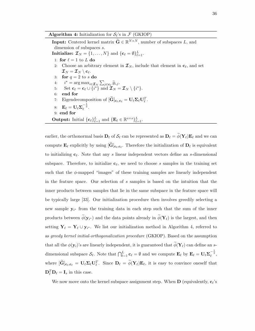
36
Algorithm 4: Initialization for S`’s in F (GKIOP)
Input: Centered kernel matrix G ∈ RN×N , number of subspaces L, anddimension of subspaces s.
Initialize: IN = 1, . . . , N and c` = ∅L`=1.
1: for ` = 1 to L do2: Choose an arbitrary element in IN , include that element in c`, and set
IN = IN \ c`.3: for q = 2 to s do4: i∗ = arg maxi∈IN
∑j∈c`
gi,j .5: Set c` = c` ∪ i∗ and IN = IN \ i∗.6: end for7: Eigendecomposition of [G]c`,c` = U`Σ`U
T` .
8: E` = U`Σ− 1
2` .
9: end for
Output: Initial c`L`=1 and E` ∈ Rs×sL`=1.
earlier, the orthonormal basis D` of S` can be represented as D` = φ(Y`)E` and we can
compute E` explicitly by using [G]c`,c` . Therefore the initialization of D` is equivalent
to initializing c`. Note that any s linear independent vectors define an s-dimensional
subspace. Therefore, to initialize c`, we need to choose s samples in the training set
such that the φ-mapped “images” of these training samples are linearly independent
in the feature space. Our selection of s samples is based on the intuition that the
inner products between samples that lie in the same subspace in the feature space will
be typically large [33]. Our initialization procedure then involves greedily selecting a
new sample yi∗ from the training data in each step such that the sum of the inner
products between φ(yi∗) and the data points already in φ(Y`) is the largest, and then
setting Y` = Y` ∪ yi∗ . We list our initialization method in Algorithm 4, referred to
as greedy kernel initial-orthogonalization procedure (GKIOP). Based on the assumption
that all the φ(yi)’s are linearly independent, it is guaranteed that φ(Y`) can define an s-
dimensional subspace S`. Note that⋂L`=1 c` = ∅ and we compute E` by E` = U`Σ
− 12
` ,
where [G]c`,c` = U`Σ`UT` . Since D` = φ(Y`)E`, it is easy to convince oneself that
DT` D` = Is in this case.
We now move onto the kernel subspace assignment step. When D (equivalently, c`’s

37
and E`’s) is fixed, kernel subspace assignment corresponds to first solving ∀i = 1, . . . , N ,
li = arg min`=1,...,L
‖φ(yi)− PS` φ(yi)‖22 = arg min`=1,...,L
κ(yi,yi)− ‖ET` ψ`(yi)‖22, (3.8)
and then setting wli,i = 1 and w`,i = 0 ∀` 6= li. Next, for the kernel subspace update
stage, since W is fixed, all the c`’s and Y`’s are fixed. By writing D` = φ(Y`)E`,
minimization of (3.5) for a fixed W can be written as a function of E`’s as follows:
minE`
f3(E1, . . . ,EL) =
L∑`,p=1` 6=p
‖φ(Y`)E` − PSp(φ(Y`)E`)‖2F
+ λ
L∑`=1
(‖φ(Y`)‖2F − ‖ET
` φ(Y`)T φ(Y`)‖2F
)s.t. ET
` [G]c`,c`E` = Is, ` = 1, 2, . . . , L. (3.9)
Instead of updating all the E`’s simultaneously, which is again a difficult optimiza-
tion problem, we use BCD to minimize f3 and update E`’s sequentially. Unlike MC-UoS
learning, however, we have to be careful here since the number of samples in Y that be-
long to Y` (i.e., N`) may change after each subspace assignment step. In particular, we
first need to initialize all the E`’s such that E` ∈ RN`×s and ET` [G]c`,c`E` = Is. To do so,
we again apply eigendecomposition of [G]c`,c` = U`Σ`UT` with the diagonal entries of
Σ` in nonincreasing order. Then we define Is = 1, . . . , s and E` = [U`]:,Is [Σ`]− 1
2Is,Is .
After this bases initialization step, we are ready to update E`’s sequentially and after
some manipulations, each BCD subproblem of (3.9) can be expressed as
E` = arg minQ:QT [G]c`,c`Q=Is
∑p 6=`‖φ(Y`)Q− PSp(φ(Y`)Q)‖2F
+λ
2(‖φ(Y`)‖2F − ‖QT φ(Y`)
T φ(Y`)‖2F )
= arg maxQ:QT [G]c`,c`Q=Is
tr(QTA`Q), (3.10)
where A` =∑
p 6=` [G]c`,cpEpETp [G]cp,c` + λ
2 [G]2c`,c` is a symmetric matrix of dimension
N` ×N`. Note that (3.10) has a similar intuitive interpretation as (2.7). When λ = 0,
(3.10) reduces to the problem of finding a subspace that is closest to the remaining
L− 1 subspaces in the feature space. When λ =∞, (3.10) reduces to the kernel PCA
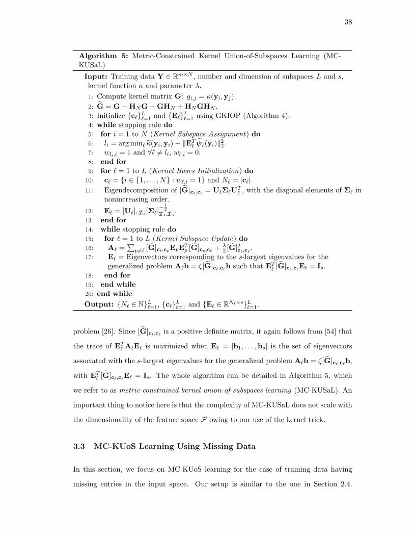
38
Algorithm 5: Metric-Constrained Kernel Union-of-Subspaces Learning (MC-KUSaL)
Input: Training data Y ∈ Rm×N , number and dimension of subspaces L and s,kernel function κ and parameter λ.
1: Compute kernel matrix G: gi,j = κ(yi,yj).
2: G = G−HNG−GHN + HNGHN .3: Initialize c`L`=1 and E`L`=1 using GKIOP (Algorithm 4).4: while stopping rule do5: for i = 1 to N (Kernel Subspace Assignment) do6: li = arg min` κ(yi,yi)− ‖ET
` ψ`(yi)‖22.7: wli,i = 1 and ∀` 6= li, w`,i = 0.8: end for9: for ` = 1 to L (Kernel Bases Initialization) do
10: c` = i ∈ 1, . . . , N : w`,i = 1 and N` = |c`|.11: Eigendecomposition of [G]c`,c` = U`Σ`U
T` , with the diagonal elements of Σ` in
nonincreasing order.
12: E` = [U`]:,Is [Σ`]− 1
2Is,Is .
13: end for14: while stopping rule do15: for ` = 1 to L (Kernel Subspace Update) do16: A` =
∑p 6=` [G]c`,cpEpE
Tp [G]cp,c` + λ
2 [G]2c`,c` .17: E` = Eigenvectors corresponding to the s-largest eigenvalues for the
generalized problem A`b = ζ[G]c`,c`b such that ET` [G]c`,c`E` = Is.
18: end for19: end while20: end while
Output: N` ∈ NL`=1, c`L`=1 and E` ∈ RN`×sL`=1.
problem [26]. Since [G]c`,c` is a positive definite matrix, it again follows from [54] that
the trace of ET` A`E` is maximized when E` = [b1, . . . ,bs] is the set of eigenvectors
associated with the s-largest eigenvalues for the generalized problem A`b = ζ[G]c`,c`b,
with ET` [G]c`,c`E` = Is. The whole algorithm can be detailed in Algorithm 5, which
we refer to as metric-constrained kernel union-of-subspaces learning (MC-KUSaL). An
important thing to notice here is that the complexity of MC-KUSaL does not scale with
the dimensionality of the feature space F owing to our use of the kernel trick.
3.3 MC-KUoS Learning Using Missing Data
In this section, we focus on MC-KUoS learning for the case of training data having
missing entries in the input space. Our setup is similar to the one in Section 2.4.

39
That is, for i = 1, . . . , N , we observe yi only at locations Ωi ⊂ 1, . . . ,m. In the
following, the resulting observed vector of yi is denoted by [yi]Ωi ∈ R|Ωi|. Also, we
assume that the observed indices of each signal, Ωi, are drawn uniformly at random
with replacement from 1, . . . ,m. Note that the results derived in here can also be
translated to the case of sampling Ωi without replacement (we refer the reader to [65,
Lemma 1] as an example). Given the missing data aspect of this setup and the kernel
trick, it is clear that we cannot apply the method in Section 2.4 for MC-KUoS learning.
However, as described in Section 3.2, the solution to the MC-KUoS learning problem
using complete data only requires computations of the inner products in F . In this
regard, we propose an estimate of the kernel function value κ(yi,yj) using incomplete
data [yi]Ωi and [yj ]Ωj . Mathematically, our goal is to find a proxy function h(·, ·)
such that h([yi]Ωi , [yj ]Ωj ) ≈ κ(yi,yj). To derive this proxy function, we start by
considering the relationship between [yi]Ωi , [yj ]Ωj and yi,yj in the context of different
kernel functions.
We first consider isotropic kernels of the form κ(yi,yj) = k(‖yi − yj‖22) for our
analysis. To begin, we define z−ij = yi − yj and Ωij = Ωi ∩Ωj , resulting in [z−ij ]Ωij =
[yi]Ωij − [yj ]Ωij ∈ R|Ωij |. For any vector z−ij , the authors in [59] define the coherence
of a subspace spanned by a vector z−ij to be µ(z−ij) =m‖z−ij‖
2∞
‖z−ij‖22and show that ‖[z−ij ]Ωij‖22
is close to|Ωij |m ‖z
−ij‖22 with high probability. Leveraging this result, we can give the
following corollary that is essentially due to [59, Lemma 1] by plugging in the definition
of z−ij and [z−ij ]Ωij .
Corollary 1. Let δ > 0, Ωij = Ωi ∩ Ωj and α =√
2µ(yi−yj)2
|Ωij | log(1δ ). Then with
probability at least 1− 2δ,
(1− α)‖yi − yj‖22 ≤m
|Ωij |‖[z−ij ]Ωij‖22 ≤ (1 + α)‖yi − yj‖22. (3.11)
Using this simple relationship in Corollary 1, we can replace the distance term
‖yi − yj‖22 in any isotropic kernel function by m|Ωij |‖[yi]Ωij − [yj ]Ωij‖22 and provide an
estimate of its true value κ(yi,yj) using entries of yi and yj that correspond to Ωij only.
For example, for the Gaussian kernel κ(yi,yj) = exp(−‖yi−yj‖22c ) with c > 0, we can
replace κ(yi,yj) with h([yi]Ωi , [yj ]Ωj ) = exp(−m‖[yi]Ωij−[yj ]Ωij ‖
22
|Ωij |c ) in our algorithms. In
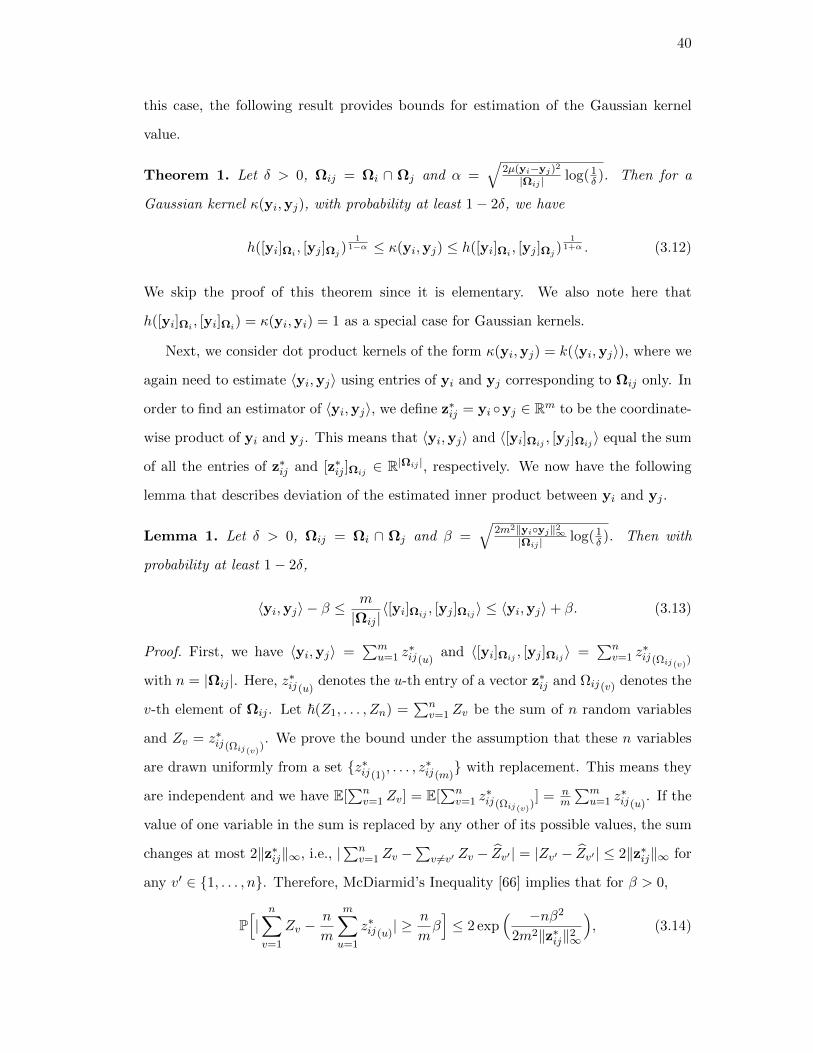
40
this case, the following result provides bounds for estimation of the Gaussian kernel
value.
Theorem 1. Let δ > 0, Ωij = Ωi ∩ Ωj and α =√
2µ(yi−yj)2
|Ωij | log(1δ ). Then for a
Gaussian kernel κ(yi,yj), with probability at least 1− 2δ, we have
h([yi]Ωi , [yj ]Ωj )1
1−α ≤ κ(yi,yj) ≤ h([yi]Ωi , [yj ]Ωj )1
1+α . (3.12)
We skip the proof of this theorem since it is elementary. We also note here that
h([yi]Ωi , [yi]Ωi) = κ(yi,yi) = 1 as a special case for Gaussian kernels.
Next, we consider dot product kernels of the form κ(yi,yj) = k(〈yi,yj〉), where we
again need to estimate 〈yi,yj〉 using entries of yi and yj corresponding to Ωij only. In
order to find an estimator of 〈yi,yj〉, we define z∗ij = yi yj ∈ Rm to be the coordinate-
wise product of yi and yj . This means that 〈yi,yj〉 and 〈[yi]Ωij , [yj ]Ωij 〉 equal the sum
of all the entries of z∗ij and [z∗ij ]Ωij ∈ R|Ωij |, respectively. We now have the following
lemma that describes deviation of the estimated inner product between yi and yj .
Lemma 1. Let δ > 0, Ωij = Ωi ∩ Ωj and β =√
2m2‖yiyj‖2∞|Ωij | log(1
δ ). Then with
probability at least 1− 2δ,
〈yi,yj〉 − β ≤m
|Ωij |〈[yi]Ωij , [yj ]Ωij 〉 ≤ 〈yi,yj〉+ β. (3.13)
Proof. First, we have 〈yi,yj〉 =∑m
u=1 z∗ij(u)
and 〈[yi]Ωij , [yj ]Ωij 〉 =∑n
v=1 z∗ij(Ωij(v))
with n = |Ωij |. Here, z∗ij(u)denotes the u-th entry of a vector z∗ij and Ωij(v) denotes the
v-th element of Ωij . Let ~(Z1, . . . , Zn) =∑n
v=1 Zv be the sum of n random variables
and Zv = z∗ij(Ωij(v)). We prove the bound under the assumption that these n variables
are drawn uniformly from a set z∗ij(1), . . . , z∗ij(m)
with replacement. This means they
are independent and we have E[∑n
v=1 Zv] = E[∑n
v=1 z∗ij(Ωij(v))
] = nm
∑mu=1 z
∗ij(u)
. If the
value of one variable in the sum is replaced by any other of its possible values, the sum
changes at most 2‖z∗ij‖∞, i.e., |∑n
v=1 Zv −∑
v 6=v′ Zv − Zv′ | = |Zv′ − Zv′ | ≤ 2‖z∗ij‖∞ for
any v′ ∈ 1, . . . , n. Therefore, McDiarmid’s Inequality [66] implies that for β > 0,
P[|n∑v=1
Zv −n
m
m∑u=1
z∗ij(u)| ≥ n
mβ]≤ 2 exp
( −nβ2
2m2‖z∗ij‖2∞
), (3.14)
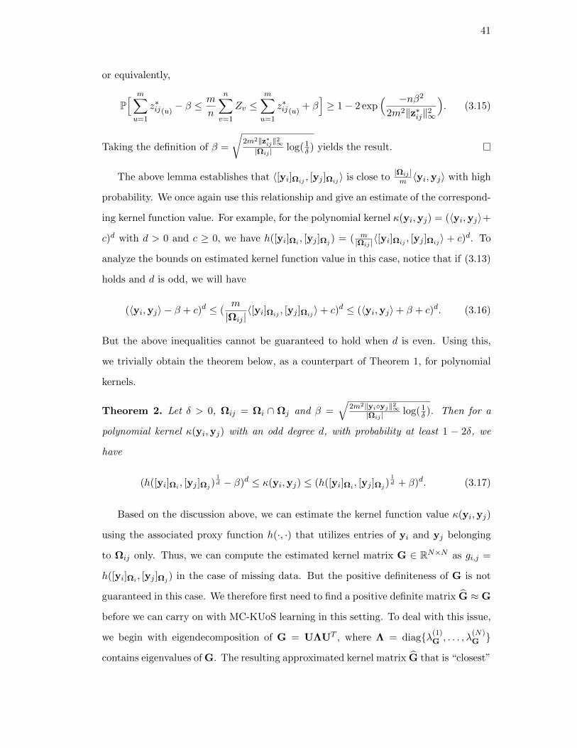
41
or equivalently,
P[ m∑u=1
z∗ij(u)− β ≤ m
n
n∑v=1
Zv ≤m∑u=1
z∗ij(u)+ β
]≥ 1− 2 exp
( −nβ2
2m2‖z∗ij‖2∞
). (3.15)
Taking the definition of β =
√2m2‖z∗ij‖2∞|Ωij | log(1
δ ) yields the result.
The above lemma establishes that 〈[yi]Ωij , [yj ]Ωij 〉 is close to|Ωij |m 〈yi,yj〉 with high
probability. We once again use this relationship and give an estimate of the correspond-
ing kernel function value. For example, for the polynomial kernel κ(yi,yj) = (〈yi,yj〉+
c)d with d > 0 and c ≥ 0, we have h([yi]Ωi , [yj ]Ωj ) = ( m|Ωij |〈[yi]Ωij , [yj ]Ωij 〉 + c)d. To
analyze the bounds on estimated kernel function value in this case, notice that if (3.13)
holds and d is odd, we will have
(〈yi,yj〉 − β + c)d ≤ (m
|Ωij |〈[yi]Ωij , [yj ]Ωij 〉+ c)d ≤ (〈yi,yj〉+ β + c)d. (3.16)
But the above inequalities cannot be guaranteed to hold when d is even. Using this,
we trivially obtain the theorem below, as a counterpart of Theorem 1, for polynomial
kernels.
Theorem 2. Let δ > 0, Ωij = Ωi ∩ Ωj and β =√
2m2‖yiyj‖2∞|Ωij | log(1
δ ). Then for a
polynomial kernel κ(yi,yj) with an odd degree d, with probability at least 1 − 2δ, we
have
(h([yi]Ωi , [yj ]Ωj )1d − β)d ≤ κ(yi,yj) ≤ (h([yi]Ωi , [yj ]Ωj )
1d + β)d. (3.17)
Based on the discussion above, we can estimate the kernel function value κ(yi,yj)
using the associated proxy function h(·, ·) that utilizes entries of yi and yj belonging
to Ωij only. Thus, we can compute the estimated kernel matrix G ∈ RN×N as gi,j =
h([yi]Ωi , [yj ]Ωj ) in the case of missing data. But the positive definiteness of G is not
guaranteed in this case. We therefore first need to find a positive definite matrix G ≈ G
before we can carry on with MC-KUoS learning in this setting. To deal with this issue,
we begin with eigendecomposition of G = UΛUT , where Λ = diagλ(1)G , . . . , λ
(N)G
contains eigenvalues of G. The resulting approximated kernel matrix G that is “closest”
42
to G can then be calculated by G = UΛUT , where Λ = diagλ(1)
G, . . . , λ
(N)
G and each
λ(i)
G, i = 1, . . . , N , is defined as
λ(i)
G=
λ
(i)G , λ
(i)G > 0
δmin, λ(i)G = 0
−λ(i)G , λ
(i)G < 0.
Here, δmin > 0 is a predefined (small) parameter. Using the above procedure, one can
obtain a positive definite matrix G such that gi,j ≈ κ(yi,yj) and use it for MC-UoS
learning in the feature space. Effectively, MC-KUoS learning in the presence of missing
data also relies on Algorithm 5, with the difference being that we use gi,j , obtained from
h([yi]Ωi , [yj ]Ωj ), in lieu of κ(yi,yj) in the overall learning process, which includes both
kernel subspace assignment and kernel subspace update stages. We dub this approach
robust MC-KUoS learning (rMC-KUSaL). We conclude this section by noting that we
can also robustify classical kernel PCA by using G as a means of performing kernel
PCA with missing data, which we call rKPCA in our experiments.
3.4 Pre-Image Reconstruction
Thus far in this chapter, we have discussed MC-UoS learning in the kernel space with
complete and missing data using the kernel trick. Now suppose we are given a new noisy
(test) sample z = x + ξ ∈ Rm, where ξ is a noise term and φ(x) = φ(x) − φ belongs
to one of the subspaces in ML (i.e., φ(x) ∈ Sτ , τ ∈ 1, . . . , L). In most information
processing tasks, one needs to first find a representation of this sample z in terms of the
learned MC-KUoS, which is akin to “denoising” z. The “denoised sample” in the feature
space is the projection of φ(z) onto Sτ , which is given by PSτφ(z) = DτDTτ φ(z)+φ with
φ(z) = φ(z)− φ. However, in order to visualize the “denoised” sample in the ambient
space, we often need to project PSτφ(z) onto the input space in many applications [6,67],
which is termed pre-image reconstruction. In this section, we consider the problem of
pre-image reconstruction based on the MC-KUoS model.
Mathematically, the problem of pre-image reconstruction can be stated as follows.
We are given z ∈ Rm and we are interested in finding z ∈ Rm whose mapping to the

43
feature space is closest to the projection of φ(z) onto the learned MC-UoS in F . This
involves first finding the index τ such that τ = arg min` ‖φ(z) − PS` φ(z)‖22, which can
be easily done using the kernel subspace assignment step described in (3.8). Next, we
need to solve z = arg min%∈Rm ‖φ(%) − PSτφ(z)‖22. To solve this problem, we leverage
the ideas in [64,68] that only use feature-space distances to find z (equivalently, to find
the pre-image of PSτφ(z)). We first study this problem when the training samples Y
are complete.
3.4.1 Pre-Image Reconstruction Using Complete Data
We first calculate the squared “feature distance” between PSτφ(z) and any φ(yi), i =
1 . . . , N , defined as [64]
d2F (φ(yi), PSτφ(z)) = ‖PSτφ(z)‖22 + ‖φ(yi)‖22 − 2(PSτφ(z))Tφ(yi). (3.18)
Notice that ‖PSτφ(z)‖22 and (PSτφ(z))Tφ(yi) can be calculated in terms of kernel rep-
resentation as follows:
‖PSτφ(z)‖22
= φ(z)TDτDTτ φ(z) + φ
Tφ+ 2φ(z)TDτD
Tτ φ
= φ(z)T φ(Yτ )EτETτ φ(Yτ )T φ(z) +
1
N21TNG1N +
2
Nφ(z)T φ(Yτ )EτE
Tτ φ(Yτ )Tφ(Y)1N
= ψτ (z)TEτETτ
(ψτ (z) +
2
N[G]cτ ,:1N −
2
N21Nτ1
TNG1N
)+
1
N21TNG1N ,
and
(PSτφ(z))Tφ(yi) = ψτ (z)TEτETτ
(ψτ (yi)−
1
N1Nτ1
TNkyi
)+
1
N1TNkyi . (3.19)
Therefore, (3.18) becomes
d2F (φ(yi), PSτφ(z)) = ψτ (z)TEτE
Tτ
(ψτ (z) +
2
N[G]cτ ,:1N − 2ψτ (yi)
− 2
N21Nτ1
TNG1N +
2
N1Nτ1
TNkyi
)+ gi,i
+1
N21TNG1N −
2
N1TNkyi
with gi,i = κ(yi,yi).
44
We now describe our method for pre-image reconstruction using the Gaussian kernel
κ(yi,yj) = exp(−‖yi−yj‖22c ) first. In this case, the problem of minimizing ‖φ(z) −
PSτφ(z)‖22 is equivalent to maximizing the function ρ(z) = (PSτφ(z))Tφ(z) [6], whose
extremum can be obtained by setting ∇zρ = 0, where ∇zρ denotes the gradient of ρ
with respect to z. To do so, we express ρ(z) as
ρ(z) = (DτDTτ φ(z) + φ)Tφ(z)
= φ(z)T φ(Yτ )EτETτ φ(Yτ )Tφ(z) +
1
N1TNφ(Y)Tφ(z)
= ψτ (z)TEτETτ (ψτ (z)− 1
N1Nτ1
TNkz) +
1
N1TNkz
= ζτ (z)T (ψτ (z)− 1
N1Nτ1
TNkz) +
1
N1TNkz, (3.20)
where ζτ (z) = EτETτ ψτ (z) ∈ R|Nτ |. Next, we define χ = 1
N (1 − ζτ (z)T1Nτ )1N ∈ RN
and let χ be an N -dimensional vector such that [χ]cτ = [χ]cτ + ζτ (z) and [χ]IN\cτ =
[χ]IN\cτ (recall that IN = 1, . . . , N and cτ contains all the indices of φ(yi)’s that are
assigned to Sτ ), which means ρ(z) = χTkz =∑N
i=1 χ(i)κ(z,yi). By setting ∇zρ = 0,
we get
z =
∑Ni=1 χ(i) exp(−‖z− yi‖22/c)yi∑Ni=1 χ(i) exp(−‖z− yi‖22/c)
. (3.21)
By using the approximation PSτφ(z) ≈ φ(z) and the relation ‖z− yi‖22 = −c log(12(2−
d2F (φ(yi), φ(z)))) [64], a unique pre-image can now be obtained by the following formula:
z =
∑Ni=1 χ(i)
(12
(2− d2
F (φ(yi), PSτφ(z))))
yi∑Ni=1 χ(i)
(12
(2− d2
F (φ(yi), PSτφ(z)))) . (3.22)
Next, for the polynomial kernel κ(yi,yj) = (〈yi,yj〉+ c)d with an odd degree d, we
can follow a similar procedure and have the following expression for an approximate
solution for pre-image reconstruction:
z =N∑i=1
χ(i)
((PSτφ(z))Tφ(yi)
‖PSτφ(z)‖22
) d−1d
yi. (3.23)
3.4.2 Pre-Image Reconstruction Using Missing Data
We next consider the problem of reconstructing the pre-image of PSτφ(z) when the
training samples have missing entries. As can be easily seen from (3.22), the solution
45
of a pre-image for the Gaussian kernel can be written as z =∑Ni=1 eiyi∑Ni=1 ei
, where ei =
χ(i)
(12(2 − d2
F (PSτφ(z), φ(yi)))). Similarly, from (3.23), we can also write the solution
of z to be z =∑N
i=1 eiyi for the polynomial kernel, where ei = χ(i)
( (PSτ φ(z))Tφ(yi)
‖PSτ φ(z)‖22
) d−1d
in this case. In words, the pre-image solution is a linear combination of the training
data, where the weights ei’s can be explicitly computed using the respective kernel
functions. In this regard, as described in Section 3.3, for each i = 1, . . . , N , we can
estimate κ(z,yi) using entries of z belonging to Ωi (i.e., [z]Ωi) and [yi]Ωi , where the
estimated kernel function value is denoted by h(z, [yi]Ωi).
Based on the estimated kernel function values h(z, [yi]Ωi)’s, we can then find the
solution of τ such that τ = arg min` ‖φ(z) − PS` φ(z)‖22, and calculate the weights ei’s
(i = 1, . . . , N). Note that unlike the complete data case, we do need to compute the
entries of z separately in this case. To be specific, for the u-th entry of z, u = 1, . . . ,m,
we define ru to be the set containing the indices of the samples yi’s whose u-th entry are
observed. Then z(u) =∑i∈ru
eiyi(u)
(∑Ni=1 ei)|ru|/N
for the Gaussian kernel and z(u) =∑
i∈rueiyi(u) for
the polynomial kernel. We conclude this section by noting that the methods described
in here can also be applied to the case when the test sample z has missing entries.
3.5 Experimental Results
In this section, we evaluate the performance of the MC-KUoS learning approaches in
terms of the following two problems: image denoising using the learned MC-KUoS and
clustering of training data points. For both these problems, we consider the USPS
dataset [69], which contains a collection of m = 256-dimensional handwritten digits.
The authors in [6] have demonstrated that using nonlinear features can improve the
denoising performance of this dataset. Unlike the experiments for MC-UoS learning, the
training data we use in this set of experiments are noiseless. For denoising experiments,
we assume every noisy test sample z = x + ξ, where φ(x) = φ(x) − φ belongs to one
of the S`’s in F (again ‖x‖22 = 1) and ξ has N (0, (σ2te/m)Im) distribution. In these
experiments, σ2te ranges from 0.2 to 0.5.
46
3.5.1 Experiments on Image Denoising
For denoising experiments, we compare the result of MC-KUSaL with three other meth-
ods: (i) kernel k-means clustering (kernel k-means) [15], where for each test signal z,
we first assign φ(z) to a cluster whose centroid is closest to φ(z) in F , followed by kernel
PCA and the method in [68] to calculate the pre-image; (ii) kernel PCA [26] with the
same number of eigenvectors as in MC-KUSaL (KPCA-Fix); and (iii) kernel PCA with
the number of eigenvectors chosen by s = arg mins ||PSφ(z)− φ(x)||22 (KPCA-Oracle),
where x and z are clean and noisy test samples, respectively. In this manner, the num-
ber of eigenvectors s for KPCA-Oracle will be different for different noise levels σte’s.
We use the same dimension of the subspaces for MC-KUSaL, kernel k-means clustering
and KPCA-Fix, while the number of subspaces L for kernel k-means clustering also
equals the one for MC-KUSaL. For the case of missing training data, we report the
results of rMC-KUSaL as well as rKPCA. For every fixed test noise level σte, we set the
dimension of the subspace s for rKPCA to be the same as the one for KPCA-Oracle.
The relative reconstruction error of a clean test signal x ∈ Xte is calculated by‖x−z‖22‖x‖22
,
where z denotes the pre-image with respect to the noisy test sample z.
We experiment with Gaussian kernel with parameter c = 4. We choose the digits
“0” and “4” and for each digit we select the first 200 samples in the dataset (400 images
in total) for our experiments. All these 400 samples are then vectorized and normalized
to unit `2 norms. From these samples, we randomly choose 120 samples (without
replacement) from each class for training and the remaining 80 samples of each class
for testing, forming X ∈ R256×240 and Xte ∈ R256×160. This random selection of test
and training samples is repeated 20 times for cross-validation purposes. We perform
10 Monte Carlo trials for noisy test data and report the mean over these 200 random
trials.
In these experiments, we implement MC-KUSaL with parameters L = 2, s = 45 and
λ ∈ 1, 4, 20, 100 to learn an MC-UoS in the feature space F . Fig. 3.1(a) shows the
mean of relative reconstruction errors of test data for different methods in the presence
of complete training data, where we use the result of MC-KUSaL with λ = 4 for
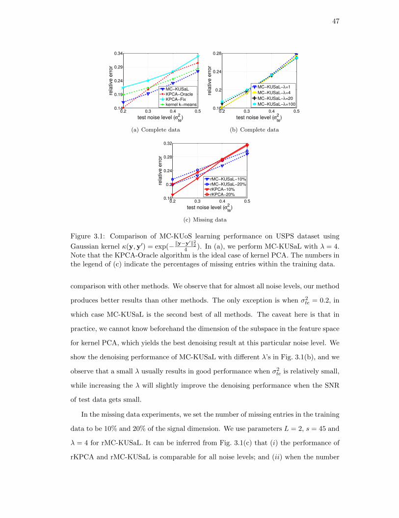
47
0.2 0.3 0.4 0.50.14
0.19
0.24
0.29
0.34
test noise level (σte
2)
rela
tive e
rror
MC−KUSaLKPCA−OracleKPCA−Fixkernel k−means
(a) Complete data
0.2 0.3 0.4 0.50.16
0.2
0.24
0.28
test noise level (σte
2)
rela
tive e
rror
MC−KUSaL−λ=1
MC−KUSaL−λ=4
MC−KUSaL−λ=20
MC−KUSaL−λ=100
(b) Complete data
0.2 0.3 0.4 0.50.16
0.2
0.24
0.28
0.32
test noise level (σte
2)
rela
tive e
rror
rMC−KUSaL−10%rMC−KUSaL−20%rKPCA−10%rKPCA−20%
(c) Missing data
Figure 3.1: Comparison of MC-KUoS learning performance on USPS dataset using
Gaussian kernel κ(y,y′) = exp(−‖y−y′‖224 ). In (a), we perform MC-KUSaL with λ = 4.
Note that the KPCA-Oracle algorithm is the ideal case of kernel PCA. The numbers inthe legend of (c) indicate the percentages of missing entries within the training data.
comparison with other methods. We observe that for almost all noise levels, our method
produces better results than other methods. The only exception is when σ2te = 0.2, in
which case MC-KUSaL is the second best of all methods. The caveat here is that in
practice, we cannot know beforehand the dimension of the subspace in the feature space
for kernel PCA, which yields the best denoising result at this particular noise level. We
show the denoising performance of MC-KUSaL with different λ’s in Fig. 3.1(b), and we
observe that a small λ usually results in good performance when σ2te is relatively small,
while increasing the λ will slightly improve the denoising performance when the SNR
of test data gets small.
In the missing data experiments, we set the number of missing entries in the training
data to be 10% and 20% of the signal dimension. We use parameters L = 2, s = 45 and
λ = 4 for rMC-KUSaL. It can be inferred from Fig. 3.1(c) that (i) the performance of
rKPCA and rMC-KUSaL is comparable for all noise levels; and (ii) when the number
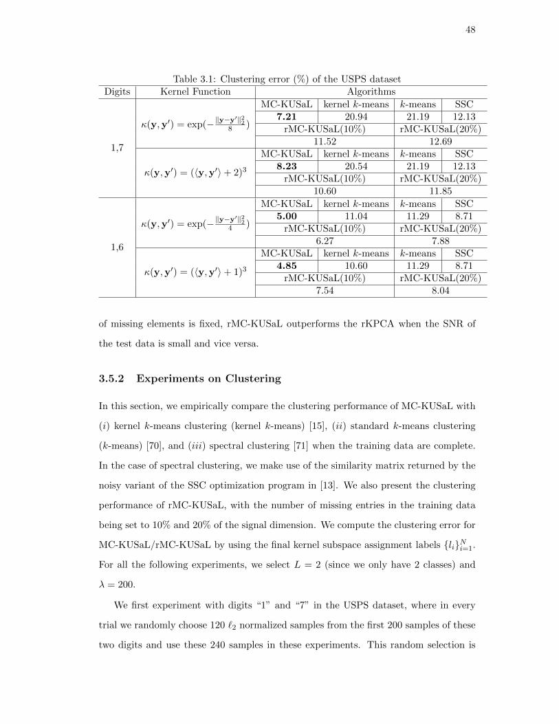
48
Table 3.1: Clustering error (%) of the USPS datasetDigits Kernel Function Algorithms
1,7
κ(y,y′) = exp(−‖y−y′‖228 )
MC-KUSaL kernel k-means k-means SSC7.21 20.94 21.19 12.13
rMC-KUSaL(10%) rMC-KUSaL(20%)11.52 12.69
κ(y,y′) = (〈y,y′〉+ 2)3
MC-KUSaL kernel k-means k-means SSC8.23 20.54 21.19 12.13
rMC-KUSaL(10%) rMC-KUSaL(20%)10.60 11.85
1,6
κ(y,y′) = exp(−‖y−y′‖224 )
MC-KUSaL kernel k-means k-means SSC5.00 11.04 11.29 8.71
rMC-KUSaL(10%) rMC-KUSaL(20%)6.27 7.88
κ(y,y′) = (〈y,y′〉+ 1)3
MC-KUSaL kernel k-means k-means SSC4.85 10.60 11.29 8.71
rMC-KUSaL(10%) rMC-KUSaL(20%)7.54 8.04
of missing elements is fixed, rMC-KUSaL outperforms the rKPCA when the SNR of
the test data is small and vice versa.
3.5.2 Experiments on Clustering
In this section, we empirically compare the clustering performance of MC-KUSaL with
(i) kernel k-means clustering (kernel k-means) [15], (ii) standard k-means clustering
(k-means) [70], and (iii) spectral clustering [71] when the training data are complete.
In the case of spectral clustering, we make use of the similarity matrix returned by the
noisy variant of the SSC optimization program in [13]. We also present the clustering
performance of rMC-KUSaL, with the number of missing entries in the training data
being set to 10% and 20% of the signal dimension. We compute the clustering error for
MC-KUSaL/rMC-KUSaL by using the final kernel subspace assignment labels liNi=1.
For all the following experiments, we select L = 2 (since we only have 2 classes) and
λ = 200.
We first experiment with digits “1” and “7” in the USPS dataset, where in every
trial we randomly choose 120 `2 normalized samples from the first 200 samples of these
two digits and use these 240 samples in these experiments. This random selection is
49
repeated 20 times. We perform MC-KUSaL and rMC-KUSaL using Gaussian kernel
κ(y,y′) = exp(−‖y−y′‖228 ) with s = 35 and polynomial kernel κ(y,y′) = (〈y,y′〉 + 2)3
with s = 40. The parameter αz for SSC is set to be 20. The clustering results are
listed in Table 3.1, where we can see the clustering error for MC-KUSaL is roughly
40% of the ones for kernel/standard k-means clustering and MC-KUSaL is much better
than SSC (with 32% reduction) in these experiments. In addition, the clustering error
for rMC-KUSaL is an increasing function of the number of missing entries for both
Gaussian kernel and polynomial kernel.
As another example, we repeat the above experiments using digits “1” and “6”,
where we again apply MC-KUSaL and rMC-KUSaL using Gaussian kernel κ(y,y′) =
exp(−‖y−y′‖224 ) with s = 35 and polynomial kernel κ(y,y′) = (〈y,y′〉+ 1)3 with s = 40.
In these experiments, SSC is performed with αz = 10. From Table 3.1, we again
observe that MC-KUSaL outperforms other clustering algorithms with 42% reduction
(compared to SSC) in the clustering error. In the missing data experiments, the clus-
tering performance of rMC-KUSaL using Gaussian kernel degrades as the number of
missing entries of the data increases. When we use polynomial kernel for rMC-KUSaL,
increasing the number of entries in the missing data does not result in much degradation
of the clustering performance.
We conclude by noting that the choice of kernels in these experiments is agnostic
to the training data. Nonetheless, data-driven learning of kernels is an active area
of research, which is sometimes studied under the rubric of multiple kernel learning
[72–75]. While some of these works can be leveraged to further improve the performance
of our proposed algorithms, a careful investigation of this is beyond the scope of this
work.
50
Chapter 4
Hierarchical Union-of-Subspaces Model for Human
Activity Summarization
4.1 Motivation
The need for high-level analytics of large streams of video data has arisen in recent
years in many practical commercial, law enforcement, and military applications [38,76–
78]. Examples include human activity recognition, video summarization and indexing,
human-machine teaming, and human behavior tracking and monitoring. The human
activity recognition process requires recognizing both objects in the scene as well as
body movements to correctly identify the activity with the help of context [79]. In the
case of video summarization, one should be able to semantically segment and summarize
the visual content in terms of context. This enables efficient indexing of large amounts
of video data, which allows for easy query and retrieval [80]. For effective human-
machine (robot) teaming, autonomous systems should be able to understand human
teammates’ gestures as well as recognize various human activities taking place in the
field to gain situational awareness of the scene. Further, an important step in building
visual tracking systems is to design ontologies and vocabularies for human activity and
environment representations [81,82]. All these tasks necessitate automated learning of
movements of the human body or human action attributes.
Human activities consist of a sequence of actions that can be represented hierarchi-
cally [38] as shown in Fig. 4.1. The bottom level of the hierarchy consists of the fine
resolution description of an action, i.e., movement of the human body (e.g., right arm
moves up, left arm moves up, torso bending, and legs moving apart) and can be called
an action attribute [39]. At the middle level, a sequence of these attributes forms a
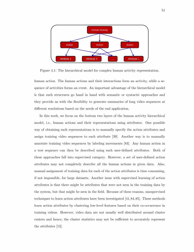
51
Human Activity
Action
Attribute L Attribute 2 Attribute 1
Action Action
…
Figure 4.1: The hierarchical model for complex human activity representation.
human action. The human actions and their interactions form an activity, while a se-
quence of activities forms an event. An important advantage of the hierarchical model
is that such structures go hand in hand with semantic or syntactic approaches and
they provide us with the flexibility to generate summaries of long video sequences at
different resolutions based on the needs of the end application.
In this work, we focus on the bottom two layers of the human activity hierarchical
model, i.e., human actions and their representations using attributes. One possible
way of obtaining such representations is to manually specify the action attributes and
assign training video sequences to each attribute [39]. Another way is to manually
annotate training video sequences by labeling movements [83]. Any human action in
a test sequence can then be described using such user-defined attributes. Both of
these approaches fall into supervised category. However, a set of user-defined action
attributes may not completely describe all the human actions in given data. Also,
manual assignment of training data for each of the action attributes is time consuming,
if not impossible, for large datasets. Another issue with supervised learning of action
attributes is that there might be attributes that were not seen in the training data by
the system, but that might be seen in the field. Because of these reasons, unsupervised
techniques to learn action attributes have been investigated [41,84,85]. These methods
learn action attributes by clustering low-level features based on their co-occurrence in
training videos. However, video data are not usually well distributed around cluster
centers and hence, the cluster statistics may not be sufficient to accurately represent
the attributes [13].
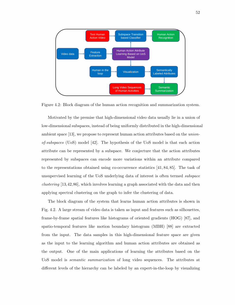
52
Video data Feature
Extraction
Human Action Attribute
Learning Based on UoS
Model
Semantically
Labeled Attributes
Human Action
Recognition
Semantic
Summarization
Human in the
loop Visualization
Test Human
Action Video
Subspace Transition
based Classifier
Long Video Sequences
of Human Activities
Figure 4.2: Block diagram of the human action recognition and summarization system.
Motivated by the premise that high-dimensional video data usually lie in a union of
low-dimensional subspaces, instead of being uniformly distributed in the high-dimensional
ambient space [13], we propose to represent human action attributes based on the union-
of-subspaces (UoS) model [42]. The hypothesis of the UoS model is that each action
attribute can be represented by a subspace. We conjecture that the action attributes
represented by subspaces can encode more variations within an attribute compared
to the representations obtained using co-occurrence statistics [41, 84, 85]. The task of
unsupervised learning of the UoS underlying data of interest is often termed subspace
clustering [13,42,86], which involves learning a graph associated with the data and then
applying spectral clustering on the graph to infer the clustering of data.
The block diagram of the system that learns human action attributes is shown in
Fig. 4.2. A large stream of video data is taken as input and features such as silhouettes,
frame-by-frame spatial features like histograms of oriented gradients (HOG) [87], and
spatio-temporal features like motion boundary histogram (MBH) [88] are extracted
from the input. The data samples in this high-dimensional feature space are given
as the input to the learning algorithm and human action attributes are obtained as
the output. One of the main applications of learning the attributes based on the
UoS model is semantic summarization of long video sequences. The attributes at
different levels of the hierarchy can be labeled by an expert-in-the-loop by visualizing

53
the first few basis vectors of each attribute (subspace) in the form of images. Once the
labeled attributes are available, any long video sequence of human activity can then be
semantically summarized at different levels of granularity based on the requirements of
an application. Another major application of learning the attributes is human action
recognition. A human action or activity can be represented as a sequence of transitions
from one attribute to another, and hence, can be represented by a subspace transition
vector. Even though multiple actions can share action attributes, each action or activity
can be uniquely represented by its subspace transition vector. A classifier can be trained
based upon these transition vectors to classify an action in a test video sequence into
one of the actions in the training data.
In this chapter, we propose a hierarchical union-of-subspaces (UoS) model to learn
human action attributes from the data at different resolutions in an unsupervised man-
ner. We use the silhouette structure of the human (after background suppression and
thresholding) as the feature in our approach. Each action attribute is represented
by a subspace built from the silhouette features. We use Sparse Subspace Clustering
(SSC) [13], a state-of-the-art subspace clustering method, as the basic subspaces learn-
ing algorithm and build our hierarchical UoS learning algorithm on top of it. Note that
in the remainder of this chapter, we use the words “subspace” and “action attribute”
interchangeably for convenience.
4.2 Background: Sparse Subspace Clustering
We start with a brief review of the Sparse Subspace Clustering (SSC) algorithm de-
scribed in [13]. Suppose we are given a collection of N signals in Rm, denoted by
Y = [y1, . . . ,yN ] ∈ Rm×N , and assume these N samples are drawn from a union of L
subspaces S`L`=1 of dimensions d`L`=1 in Rm, where every signal belongs to one of
the subspaces in S`L`=1. Therefore, we can write Y = Y1 ∪Y2 ∪ · · · ∪YL where each
Y` ∈ Rm×N` is a submatrix of Y containing all the samples that belong to subspace
S` with N` > d`, and we have∑L
`=1N` = N . Based on the intuition that each sample
yi can be expressed as a sparse linear combination of the data points from the same

54
subspace to which yi belongs, one can represent yi as follows:
ai = arg minai
‖ai‖1 s.t. yi = Yai, ai(i) = 0, (4.1)
where ai = [ai(1) , ai(2) , . . . , ai(N)]T ∈ RN is the coefficient vector and ‖ai‖1 =
∑Nj=1 |ai(j) |.
Considering all the data points in matrix form, SSC learns a sparse coefficient matrix
A = [a1, a2, . . . , aN ] ∈ RN×N by minimizing the following objective function:
A = arg minA
‖A‖1 s.t. Y = YA, diag(A) = 0, (4.2)
where diag(A) is the diagonal vector of matrix A. Using the resulting coefficient matrix
A, the segmentation of data points into respective subspaces Y1, . . . ,YL can be done
by applying spectral clustering [71] on the similarity matrix W = |A|+ |A|T , where | · |
denotes the element-wise absolute value operation. In the case when data are corrupted
by noise, SSC solves the following convex optimization problem for A:
A = arg minA
‖A‖1 + λ‖Y −YA‖2F s.t. diag(A) = 0. (4.3)
Here, λ > 0 is a regularization parameter. The authors in [13] proposed an efficient
solution for calculating the sparse coefficients A using Alternating Direction Method
of Multipliers (ADMM) [89]. Note that there also exist some other UoS learning ap-
proaches, such as robust sparse subspace clustering (RSSC) [34] and robust subspace
clustering via thresholding (TSC) [33]. In this work, we propose our hierarchical UoS
learning algorithm based on SSC due to its superior performance, although our ap-
proach is extendable to other algorithms.
4.3 Hierarchical Sparse Subspace Clustering
In this section, we introduce our Hierarchical Sparse Subspace Clustering (HSSC) algo-
rithm for learning multiple levels of UoS using a collection of high-dimensional data. We
use Yp|` ∈ Rm×Np|` to denote the set of signals that are assigned to the `-th subspace at
the p-th level of the hierarchical structure, where Np|` is the number of signals in Yp|`.
Let Lp denote the number of subspaces at the p-th level, then we have∑Lp
`=1Np|` = N
and Y =⋃Lp`=1 Yp|` for all p’s. The subspace underlying Yp|` is denoted by Sp|` and its
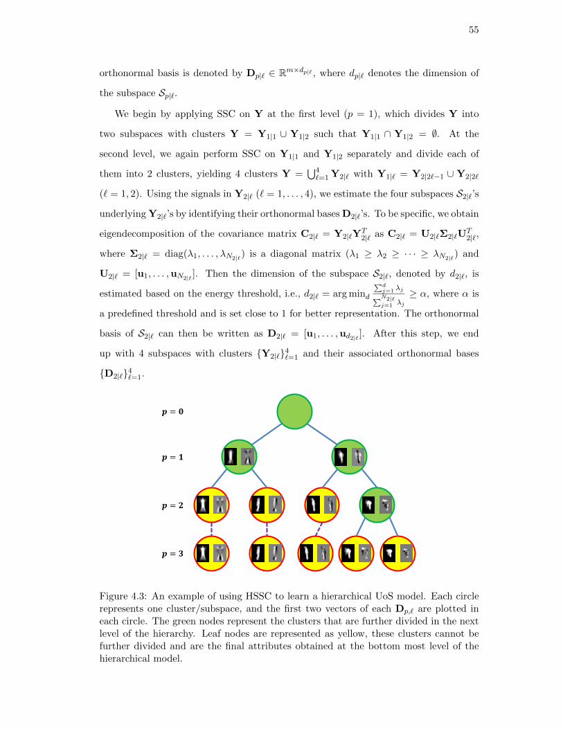
55
orthonormal basis is denoted by Dp|` ∈ Rm×dp|` , where dp|` denotes the dimension of
the subspace Sp|`.
We begin by applying SSC on Y at the first level (p = 1), which divides Y into
two subspaces with clusters Y = Y1|1 ∪ Y1|2 such that Y1|1 ∩ Y1|2 = ∅. At the
second level, we again perform SSC on Y1|1 and Y1|2 separately and divide each of
them into 2 clusters, yielding 4 clusters Y =⋃4`=1 Y2|` with Y1|` = Y2|2`−1 ∪ Y2|2`
(` = 1, 2). Using the signals in Y2|` (` = 1, . . . , 4), we estimate the four subspaces S2|`’s
underlying Y2|`’s by identifying their orthonormal bases D2|`’s. To be specific, we obtain
eigendecomposition of the covariance matrix C2|` = Y2|`YT2|` as C2|` = U2|`Σ2|`U
T2|`,
where Σ2|` = diag(λ1, . . . , λN2|`) is a diagonal matrix (λ1 ≥ λ2 ≥ · · · ≥ λN2|`) and
U2|` = [u1, . . . ,uN2|` ]. Then the dimension of the subspace S2|`, denoted by d2|`, is
estimated based on the energy threshold, i.e., d2|` = arg mind
∑dj=1 λj∑N2|`j=1 λj
≥ α, where α is
a predefined threshold and is set close to 1 for better representation. The orthonormal
basis of S2|` can then be written as D2|` = [u1, . . . ,ud2|` ]. After this step, we end
up with 4 subspaces with clusters Y2|`4`=1 and their associated orthonormal bases
D2|`4`=1.
𝒑 = 𝟎
𝒑 = 𝟏
𝒑 = 𝟐
𝒑 = 𝟑
Figure 4.3: An example of using HSSC to learn a hierarchical UoS model. Each circlerepresents one cluster/subspace, and the first two vectors of each Dp,` are plotted ineach circle. The green nodes represent the clusters that are further divided in the nextlevel of the hierarchy. Leaf nodes are represented as yellow, these clusters cannot befurther divided and are the final attributes obtained at the bottom most level of thehierarchical model.
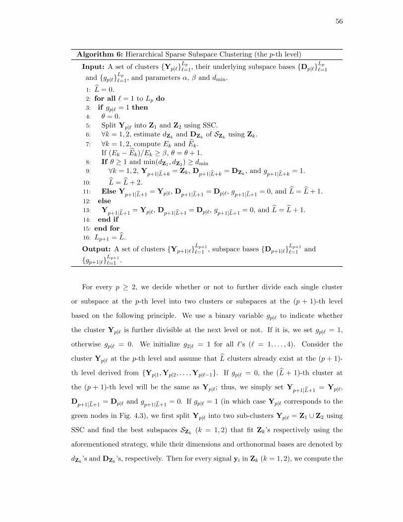
56
Algorithm 6: Hierarchical Sparse Subspace Clustering (the p-th level)
Input: A set of clusters Yp|`Lp`=1, their underlying subspace bases Dp|`
Lp`=1
and gp|`Lp`=1, and parameters α, β and dmin.
1: L = 0.2: for all ` = 1 to Lp do3: if gp|` = 1 then4: θ = 0.5: Split Yp|` into Z1 and Z2 using SSC.6: ∀k = 1, 2, estimate dZk and DZk of SZk using Zk.
7: ∀k = 1, 2, compute Ek and Ek.If (Ek − Ek)/Ek ≥ β, θ = θ + 1.
8: If θ ≥ 1 and min(dZ1 , dZ2) ≥ dmin
9: ∀k = 1, 2, Yp+1|L+k
= Zk, Dp+1|L+k
= DZk , and gp+1|L+k
= 1.
10: L = L+ 2.11: Else Y
p+1|L+1= Yp|`, D
p+1|L+1= Dp|`, gp+1|L+1
= 0, and L = L+ 1.
12: else13: Y
p+1|L+1= Yp|`, D
p+1|L+1= Dp|`, gp+1|L+1
= 0, and L = L+ 1.
14: end if15: end for16: Lp+1 = L.
Output: A set of clusters Yp+1|`Lp+1
`=1 , subspace bases Dp+1|`Lp+1
`=1 and
gp+1|`Lp+1
`=1 .
For every p ≥ 2, we decide whether or not to further divide each single cluster
or subspace at the p-th level into two clusters or subspaces at the (p + 1)-th level
based on the following principle. We use a binary variable gp|` to indicate whether
the cluster Yp|` is further divisible at the next level or not. If it is, we set gp|` = 1,
otherwise gp|` = 0. We initialize g2|` = 1 for all `’s (` = 1, . . . , 4). Consider the
cluster Yp|` at the p-th level and assume that L clusters already exist at the (p + 1)-
th level derived from Yp|1,Yp|2, . . . ,Yp|`−1. If gp|` = 0, the (L + 1)-th cluster at
the (p + 1)-th level will be the same as Yp|`; thus, we simply set Yp+1|L+1
= Yp|`,
Dp+1|L+1
= Dp|` and gp+1|L+1
= 0. If gp|` = 1 (in which case Yp|` corresponds to the
green nodes in Fig. 4.3), we first split Yp|` into two sub-clusters Yp|` = Z1 ∪ Z2 using
SSC and find the best subspaces SZk (k = 1, 2) that fit Zk’s respectively using the
aforementioned strategy, while their dimensions and orthonormal bases are denoted by
dZk ’s and DZk ’s, respectively. Then for every signal yi in Zk (k = 1, 2), we compute the
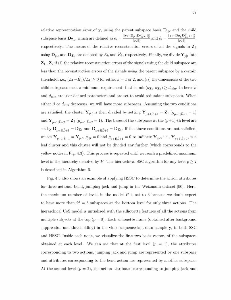
57
relative representation error of yi using the parent subspace basis Dp|` and the child
subspace basis DZk , which are defined as ei =‖yi−Dp|`D
Tp|`yi‖
22
‖yi‖22and ei =
‖yi−DZkDT
Zkyi‖22
‖yi‖22,
respectively. The means of the relative reconstruction errors of all the signals in Zk
using Dp|` and DZk are denoted by Ek and Ek, respectively. Finally, we divide Yp|` into
Z1∪Z2 if (i) the relative reconstruction errors of the signals using the child subspace are
less than the reconstruction errors of the signals using the parent subspace by a certain
threshold, i.e., (Ek−Ek)/Ek ≥ β for either k = 1 or 2, and (ii) the dimensions of the two
child subspaces meet a minimum requirement, that is, min(dZ1 , dZ2) ≥ dmin. In here, β
and dmin are user-defined parameters and are set to avoid redundant subspaces. When
either β or dmin decreases, we will have more subspaces. Assuming the two conditions
are satisfied, the cluster Yp|` is then divided by setting Yp+1|L+1
= Z1 (gp+1|L+1
= 1)
and Yp+1|L+2
= Z2 (gp+1|L+2
= 1). The bases of the subspaces at the (p+1)-th level are
set by Dp+1|L+1
= DZ1 and Dp+1|L+2
= DZ2 . If the above conditions are not satisfied,
we set Yp+1|L+1
= Yp|`, gp|` = 0 and gp+1|L+1
= 0 to indicate Yp|`, i.e., Yp+1|L+1
, is a
leaf cluster and this cluster will not be divided any further (which corresponds to the
yellow nodes in Fig. 4.3). This process is repeated until we reach a predefined maximum
level in the hierarchy denoted by P . The hierarchical SSC algorithm for any level p ≥ 2
is described in Algorithm 6.
Fig. 4.3 also shows an example of applying HSSC to determine the action attributes
for three actions: bend, jumping jack and jump in the Weizmann dataset [90]. Here,
the maximum number of levels in the model P is set to 3 because we don’t expect
to have more than 23 = 8 subspaces at the bottom level for only three actions. The
hierarchical UoS model is initialized with the silhouette features of all the actions from
multiple subjects at the top (p = 0). Each silhouette frame (obtained after background
suppression and thresholding) in the video sequence is a data sample yi in both SSC
and HSSC. Inside each node, we visualize the first two basis vectors of the subspaces
obtained at each level. We can see that at the first level (p = 1), the attributes
corresponding to two actions, jumping jack and jump are represented by one subspace
and attributes corresponding to the bend action are represented by another subspace.
At the second level (p = 2), the action attributes corresponding to jumping jack and

58
jump are separated into two different subspaces. While the action attributes of the bend
action, which is a more complex action with wider range of movement, are divided into
two subspaces, representing the more upright part of the bend action as one higher
resolution attribute and the lower part of the bend action as another higher resolution
attribute. The lower part of the bend action is further divided into two more attributes
at the next level (p = 3) while the other attributes are left as they were. Thus, we can
see that as p increases, the variations within each action can be identified, extracted
and represented using more number of higher resolution action attributes.
The proposed HSSC algorithm has some obvious advantages over flat SSC for learn-
ing human action attributes. First, in the case of flat SSC, one has to define the num-
ber of subspaces into which the data are to be clustered [13]. This requirement puts
a constraint of prior knowledge about the data in that we need to know the number
of underlying human action attributes present in the data. Such an approach moves
away from data-driven learning. On the other hand, HSSC algorithm only requires the
knowledge of a maximum level P , and it can stop before it reaches the P -th level if
no clusters can be further divided. HSSC algorithm is designed in such a way that all
the variations within each action can be identified automatically to determine the final
number of action attributes. Second, HSSC provides us with multiple resolutions of ac-
tion attributes, which are extremely useful for semantic labeling and understanding of
human actions. The multi-resolution attributes can be used for semantic summarization
of long video sequences at different resolutions starting from giving just an overview of
the action to detailed explanation of movements occurring in the video. Flat SSC can
provide us with only one set of action attributes at one single resolution, which depends
on the number of subspaces that is the input to the algorithm. The empirical results
presented in Section 4.4 illustrate these benefits of HSSC with examples.
To demonstrate the reason why HSSC outperforms flat SSC, we consider the follow-
ing example. We perform HSSC with P = 3 to learn attributes for three actions: bend,
run and one-hand wave in Weizmann dataset [90]. It has 6 subspaces as the leaf nodes,
and the first three basis vectors of each leaf subspace are illustrated in Fig. 4.4 (a)-(f).
We then apply SSC to learn 6 attributes and all those subspaces are depicted in Fig. 4.4
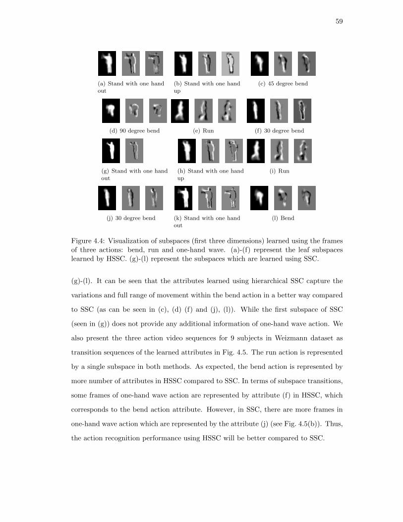
59
(a) Stand with one handout
(b) Stand with one handup
(c) 45 degree bend
(d) 90 degree bend (e) Run (f) 30 degree bend
(g) Stand with one handout
(h) Stand with one handup
(i) Run
(j) 30 degree bend (k) Stand with one handout
(l) Bend
Figure 4.4: Visualization of subspaces (first three dimensions) learned using the framesof three actions: bend, run and one-hand wave. (a)-(f) represent the leaf subspaceslearned by HSSC. (g)-(l) represent the subspaces which are learned using SSC.
(g)-(l). It can be seen that the attributes learned using hierarchical SSC capture the
variations and full range of movement within the bend action in a better way compared
to SSC (as can be seen in (c), (d) (f) and (j), (l)). While the first subspace of SSC
(seen in (g)) does not provide any additional information of one-hand wave action. We
also present the three action video sequences for 9 subjects in Weizmann dataset as
transition sequences of the learned attributes in Fig. 4.5. The run action is represented
by a single subspace in both methods. As expected, the bend action is represented by
more number of attributes in HSSC compared to SSC. In terms of subspace transitions,
some frames of one-hand wave action are represented by attribute (f) in HSSC, which
corresponds to the bend action attribute. However, in SSC, there are more frames in
one-hand wave action which are represented by the attribute (j) (see Fig. 4.5(b)). Thus,
the action recognition performance using HSSC will be better compared to SSC.

60
Frame indexes
Su
bsp
ace
assig
nm
en
t in
de
xe
s
a
b
c
d
e
f
me ind
(a)
Frame indexes
Su
bsp
ace
assig
nm
en
t in
de
xe
s
g
h
i
j
k
l
me ind
(b)
Figure 4.5: Subspace assignment result of the video frames from bend, run and one-handwave actions using subspaces learned from (a) HSSC and (b) SSC.
4.3.1 Complexity Analysis for Flat SSC and Hierarchical SSC
We first investigate the computational complexity of flat SSC. As proposed in [13],
SSC mainly consists of three steps: learning the sparse coefficients A using ADMM,
computing the normalized Laplacian matrix from A, and k-means clustering (with L
clusters) on the normalized Laplacian matrix. For the first two steps, the complexity
is implementation dependent, but the worst case would be O(N3), where N is the
number of samples in the training data Y. The complexity of k-means clustering on
the normalized Laplacian matrix is O(N2L). Therefore, by assuming L N , the
overall complexity of SSC is O(N3).
To analyze the computational complexity of hierarchical SSC, we assume that there
are 2p clusters at the p-th level (p = 0, 1, . . . , log2 L). For each cluster at the p-th level
(0 ≤ p ≤ log2 L − 1), we run SSC on each cluster to obtain two sub-clusters at the
next level. We again use Np|` to denote number of signals that are assigned to the
`-th cluster at the p-th level. As discussed earlier, the computational complexity of
applying SSC on these Np|` samples for two clusters will be O(N3p|`). For the sake of
exposition, we make another assumption that Np|` = N/2p for all `’s. In such a case,
the overall complexity at the p-th level is O((N/2p)3×2p) = O(N3/4p). The sum of the
complexity orders over all the levels gives us the overall complexity of hierarchical SSC
as∑log2 L−1
p=0 O(N3/4p) = O(43N
3(1− 1L2 )). The computational complexity of HSSC is

61
slightly more than that of flat SSC. However, the advantages of HSSC over flat SSC in
learning better action attributes at different resolutions without any prior knowledge of
the number of attributes significantly outweighs this slight increase in computational
complexity.
4.3.2 Action Recognition Using Learned Subspaces
In this section, we describe the classification strategy to perform action recognition using
the hierarchical UoS model learned by HSSC algorithm. We first learn the subspaces,
which are the action attributes, by applying HSSC on the silhouette feature sequences
of human actions in an unsupervised manner, where each silhouette frame (each data
sample) is vectorized and normalized to unit `2 norm. We assume HSSC ends up with
LP leaf subspaces and the orthonormal bases of these subspaces can be represented by
DP |` ∈ Rm×dP |`LP`=1.
Suppose there are V actions and R subjects in the training set. We use Φv,r ∈
Rm×sv,r to denote the video sequence of the r-th subject with the v-th action, where
sv,r denotes the number of frames in the video. We assign every frame in one video
sequence Φv,r (v ∈ 1, . . . , V , r ∈ 1, . . . , R) to the “closest leaf subspace” and we
use φv,r ∈ Rsv,r to denote the vector which contains the resulting subspace assignment
indexes. This vector represents the sequence of action attributes and the transitions
involved in the human action video. All training video samples have subspace tran-
sition vectors φv,r’s. Then for a test video Ψ ∈ Rm×s with s denoting the number
of frames in this video, we first perform subspace assignment for all the frames in Ψ
and we use ψ ∈ Rs to denote the resulting transition vector. Then we use a nearest
neighbor classifier to perform action recognition, i.e., Ψ is declared to be in a partic-
ular action class v′ for which the average of distances between the transition vector ψ
and all the training transition vectors φv′,r’s in the v′-th class is the smallest. Note
that the video sequences, and hence the subspace assignment vectors, are of differ-
ent lengths. In order to make the action recognition process temporal-scale invariant,
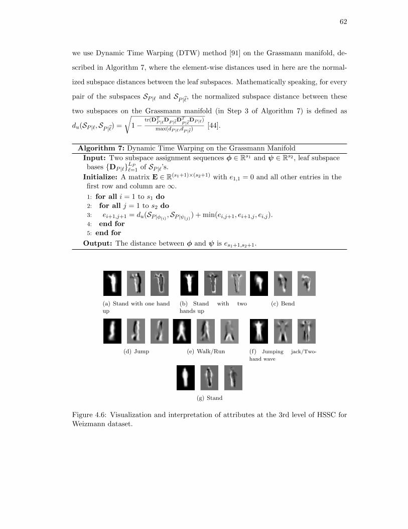
62
we use Dynamic Time Warping (DTW) method [91] on the Grassmann manifold, de-
scribed in Algorithm 7, where the element-wise distances used in here are the normal-
ized subspace distances between the leaf subspaces. Mathematically speaking, for every
pair of the subspaces SP |` and SP |, the normalized subspace distance between these
two subspaces on the Grassmann manifold (in Step 3 of Algorithm 7) is defined as
du(SP |`,SP |) =
√1−
tr(DTP |`DP |DT
P |DP |`)
max(dP |`,dP |) [44].
Algorithm 7: Dynamic Time Warping on the Grassmann Manifold
Input: Two subspace assignment sequences φ ∈ Rs1 and ψ ∈ Rs2 , leaf subspacebases DP |`LP`=1 of SP |`’s.
Initialize: A matrix E ∈ R(s1+1)×(s2+1) with e1,1 = 0 and all other entries in thefirst row and column are ∞.
1: for all i = 1 to s1 do2: for all j = 1 to s2 do3: ei+1,j+1 = du(SP |φ(i) ,SP |ψ(j)
) + min(ei,j+1, ei+1,j , ei,j).4: end for5: end for
Output: The distance between φ and ψ is es1+1,s2+1.
(a) Stand with one handup
(b) Stand with twohands up
(c) Bend
(d) Jump (e) Walk/Run (f) Jumping jack/Two-
hand wave
(g) Stand
Figure 4.6: Visualization and interpretation of attributes at the 3rd level of HSSC forWeizmann dataset.
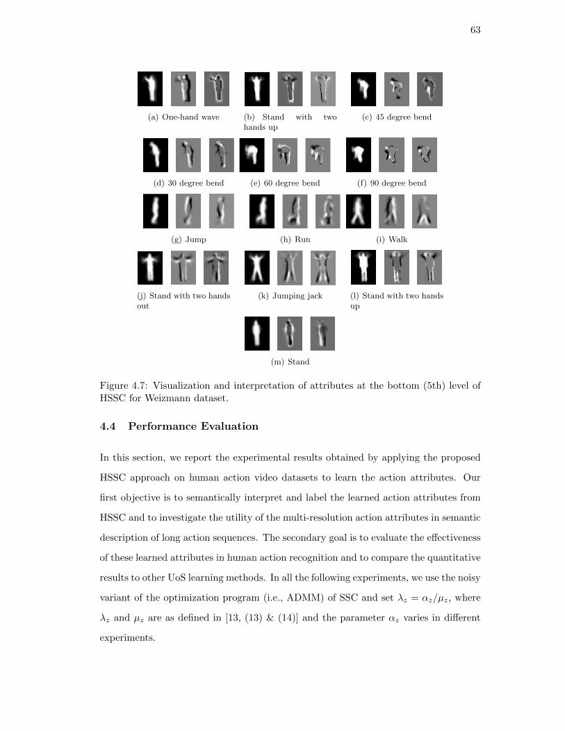
63
(a) One-hand wave (b) Stand with twohands up
(c) 45 degree bend
(d) 30 degree bend (e) 60 degree bend (f) 90 degree bend
(g) Jump (h) Run (i) Walk
(j) Stand with two handsout
(k) Jumping jack (l) Stand with two handsup
(m) Stand
Figure 4.7: Visualization and interpretation of attributes at the bottom (5th) level ofHSSC for Weizmann dataset.
4.4 Performance Evaluation
In this section, we report the experimental results obtained by applying the proposed
HSSC approach on human action video datasets to learn the action attributes. Our
first objective is to semantically interpret and label the learned action attributes from
HSSC and to investigate the utility of the multi-resolution action attributes in semantic
description of long action sequences. The secondary goal is to evaluate the effectiveness
of these learned attributes in human action recognition and to compare the quantitative
results to other UoS learning methods. In all the following experiments, we use the noisy
variant of the optimization program (i.e., ADMM) of SSC and set λz = αz/µz, where
λz and µz are as defined in [13, (13) & (14)] and the parameter αz varies in different
experiments.

64
Frame indexesSu
bsp
ace
assig
nm
en
t in
de
xe
s
d
e
f
j
l
m
Frame indexesSu
bsp
ace
assig
nm
en
t in
de
xe
s
c
f
g
Figure 4.8: Subspace transition of a long sequence using subspaces at the 5th level (top)and the 3rd level (bottom). The subspace assignment indexes in the top/bottom figurecorrespond to the attributes in Fig. 4.7 and Fig. 4.6, respectively.
4.4.1 Semantic Labeling and Summarization
In this section, we visualize the learned attributes from HSSC at two different resolu-
tions, give them semantic labels and use them for semantic summarization of multiple
actions in a long video sequence. We apply HSSC on the Weizmann dataset with pa-
rameters P = 5, α = 0.9, β = 0.05, dmin = 4 and αz = 20. HSSC returns LP = 13 leaf
subspaces at the 5th level and 7 subspaces at the 3rd level. We show the first three
dimensions of the orthonormal bases of those subspaces (attributes) here and give them
interpretative (semantic) labels in Fig. 4.7 and Fig. 4.6, respectively. To demonstrate
the semantic summarization of a long video sequence, we create a sequence by concate-
nating the bend and two-hand wave sequence of one subject and visualize the subspace
transition of the frames in Fig. 4.8. We can interpret the actions using the attribute
assignment within the interval defined by green lines based on the corresponding labels
in Fig. 4.7 and Fig. 4.6. At Level 5 (Fig. 4.8, top), human actions in the first half of
the video sequence can be described as 30 degree bend followed by 60 degree bend, 90
degree bend, 60 degree bend again, and 30 degree bend, which can be interpreted as
a full range bend action as done in Level 3 (Fig. 4.8, bottom). Next, at Level 5, the
actions in the second half of the video sequence are Stand followed by two alternating
attributes: Stand with two hands out and Stand with two hands up. The complete

65
action can be described as a two-hand wave, which is precisely what is done at a lower
resolution in Level 3. Therefore, we can say that the attributes generated at different
levels of HSSC algorithm can be used for semantic summarization of video sequences
at different resolutions.
4.4.2 Action Recognition: Evaluation on Different Datasets
In this section, we compare the performance of the proposed HSSC algorithm to flat
SSC [13], RSSC [34], and TSC [33] with the number of clusters set (i) to be the same
number of subspaces generated by HSSC at the bottom-most level (which is denoted
by Algorithm-LP ) and (ii) to be the same as the number of actions (which is denoted
by Algorithm-V ). The parameter αz for flat SSC is the same as the one for HSSC.
In the case of RSSC, we set λ = 1/√d as per [34], where d is the mean of the sub-
space dimensions returned by SSC-LP /SSC-V . The tuning parameter q in TSC is set
q = max(3, dN/(L × 20)e), where L is equal to LP and V for TSC-LP and TSC-V ,
respectively.
We use three public datasets for this purpose: the Weizmann action dataset [90], the
Keck gesture dataset [92], and the UT-Tower action dataset [93]. We evaluate all the
subspace/attribute learning approaches based on a leave-one-subject-out experiment.
To be specific, we pick all the videos of one subject (see Section 4.3.2) for testing at one
time, while using all other videos as training samples. The Weizmann dataset consists
of V = 10 different actions: walk, run, jump, gallop sideways, bend, one-hand wave,
two-hands wave, jump in place, jumping jack, and skip. Each action is performed by
nine subjects. The original resolution of the frames is 180×144. We align all the binary
silhouette sequences and crop them into 87× 63 frames, thereby the dimensionality of
data is m = 5481. The hierarchical SSC is performed with parameters described in
Section 4.4.1 and it returns LP = 13 leaf subspaces for final attributes. The Keck
gesture dataset was collected using a camera with 640 × 480 resolution. It consists of
V = 14 different actions, including turn left, turn right, attention left, attention right,
flap, stop left, stop right, stop both, attention both, start, go back, close distance, speed
up, and come near. Each of these 14 actions is performed by three people. In each video
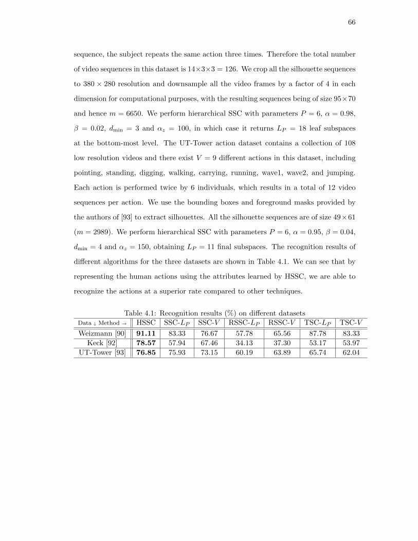
66
sequence, the subject repeats the same action three times. Therefore the total number
of video sequences in this dataset is 14×3×3 = 126. We crop all the silhouette sequences
to 380 × 280 resolution and downsample all the video frames by a factor of 4 in each
dimension for computational purposes, with the resulting sequences being of size 95×70
and hence m = 6650. We perform hierarchical SSC with parameters P = 6, α = 0.98,
β = 0.02, dmin = 3 and αz = 100, in which case it returns LP = 18 leaf subspaces
at the bottom-most level. The UT-Tower action dataset contains a collection of 108
low resolution videos and there exist V = 9 different actions in this dataset, including
pointing, standing, digging, walking, carrying, running, wave1, wave2, and jumping.
Each action is performed twice by 6 individuals, which results in a total of 12 video
sequences per action. We use the bounding boxes and foreground masks provided by
the authors of [93] to extract silhouettes. All the silhouette sequences are of size 49×61
(m = 2989). We perform hierarchical SSC with parameters P = 6, α = 0.95, β = 0.04,
dmin = 4 and αz = 150, obtaining LP = 11 final subspaces. The recognition results of
different algorithms for the three datasets are shown in Table 4.1. We can see that by
representing the human actions using the attributes learned by HSSC, we are able to
recognize the actions at a superior rate compared to other techniques.
Table 4.1: Recognition results (%) on different datasetsData ↓ Method → HSSC SSC-LP SSC-V RSSC-LP RSSC-V TSC-LP TSC-V
Weizmann [90] 91.11 83.33 76.67 57.78 65.56 87.78 83.33
Keck [92] 78.57 57.94 67.46 34.13 37.30 53.17 53.97
UT-Tower [93] 76.85 75.93 73.15 60.19 63.89 65.74 62.04

67
Chapter 5
Human Action Attribute Learning Using Low-Rank
Representations
In Chapter 4, we use the silhouette structure as the basic feature to learn action at-
tributes. However, it is almost impossible to obtain clean silhouette features in many
real applications due to cluttered background and drastic changes in the background.
On the other hand, the `1 graph built from SSC does not consider the global structure of
the data. Similar features may have drastically different coefficients for subspace clus-
tering, which will degrade the clustering performance. To capture the global structure of
data, low-rank representation (LRR) models with and without sparsity constraints have
been proposed in [94] and [42], respectively. It has been proved that LRR can achieve
perfect subspace clustering results under the condition that the subspaces underlying
the data are independent [42, 95]. However, this condition is hard to satisfy in many
real situations. To handle the case of disjoint subspaces, Tang et al. [96] extended LRR
by imposing restrictions on the structure of the solution, called structure-constrained
LRR (SC-LRR).
Existing LRR based subspace clustering techniques use spectral clustering as a post-
processing step on the graph generated from a low-rank coefficient matrix, but the
relationship between the coefficient matrix and the segmentation of data is seldom
considered, which can lead to sub-optimal results [97]. In this chapter, we propose
a hierarchical clustering-aware structure-constrained LRR (HCS-LRR) model, for un-
supervised learning of human action attributes using other low-level features such as
HOG [87] and MBH [88].

68
HOG feature
matrix
HOG feature
vector
(a)
MBH feature
matrix
MBH feature
vector
Optical flow
components
(b)
Figure 5.1: Illustration of our approach to create the matrix X for (a) HOG and (b)MBH features, which is then input to the HCS-LRR algorithm.
5.1 Feature Extraction for Attribute Learning
The main focus of our work is to learn meaningful human action attributes from large
streams of video data in an unsupervised manner. The first step in our proposed
framework is to extract feature descriptors from an action interest region in which the
human performs the action. The action interest region of each frame of an action
sequence is determined by a bounding box. In our work, we learn action attributes
using two local visual descriptors: HOG (histograms of oriented gradients) [87] and
MBH (motion boundary histogram) [88]. To extract HOG descriptors, we divide the
action interest region into a grid of blocks, each of size nσ×nσ pixels. Then HOG feature
is extracted for each block and orientations are quantized into 9 bins. Therefore, the
HOG feature of every frame can be stored into a matrix Xi ∈ Rnb×9, where nb denotes
the number of blocks in the action interest region, and the HOG feature vector of each
block corresponds to a row in Xi. We vectorize HOG features and normalize each
vector to unit `2 norm, forming individual data samples in a matrix X ∈ Rm×N , where
69
m = nb × 9 and N denotes the total number of frames in the videos, as shown in
Fig. 5.1(a).
The MBH descriptor represents the oriented gradients computed separately from
the vertical and horizontal components of the optical flow, which is robust to camera
and background motion. To extract MBH descriptors, we first split the optical flow field
into two scalar fields corresponding to the horizontal and vertical components, which
can be regarded as “images” of the motion components. Similar to HOG descriptor
extraction, we divide the action interest region of each of the optical flow component
image into a grid of blocks, each of size nσ × nσ pixels. Spatial derivatives are then
computed for each block in each optical flow component and orientation information is
quantized into 9 bins. Instead of using MBH features of optical flow field between every
two video frames separately, we aggregate MBH features of every nτ adjacent optical
flow fields (computed between nτ + 1 video frames) and the sum is used as the feature
of these nτ optical flow fields. Therefore, the MBH feature of every nτ adjacent optical
flow fields corresponds to a matrix Xi ∈ Rnb×18, where nb denotes the number of blocks
in the action interest region, and the MBH feature vector of each block corresponds
to a row in Xi. We again vectorize the MBH features and normalize each vector to
unit `2 norm, forming MBH feature matrix X ∈ Rm×N , where m = nb × 18 and N
again denotes the total number of feature descriptors, see Fig. 5.1(b). Given all the
features extracted from the video data, we aim to learn action attributes based on the
UoS model, which will be described in the following sections.
5.2 Clustering-Aware Structure-Constrained Low-Rank Representa-
tion
In this section, we propose our clustering-aware structure-constrained LRR (CS-LRR)
model for learning the action attributes using the feature descriptors extracted from
the video data. We begin with a brief review of LRR and SC-LRR since our CS-LRR
model extends these models.
70
5.2.1 Brief Review of LRR and SC-LRR
Consider a collection of N feature vectors in Rm, X = [x1,x2, . . . ,xN ], that are drawn
from a union of L low-dimensional subspaces S`L`=1 of dimensions d`L`=1. The
task of subspace clustering is to segment the data points according to their respective
subspaces. Low-rank representation (LRR) is a recently proposed subspace clustering
method [42, 95] that aims to find the lowest-rank representation for the data using a
predefined dictionary to reveal the intrinsic geometric structure of the data. Mathe-
matically, LRR can be formulated as the following optimization problem [95]:
Z = arg minZ
rank(Z) s.t. X = AZ, (5.1)
where A is a predefined dictionary that linearly spans the data space and Z is the
low-rank representation of the data over A. In practice, the observed data X are
often corrupted by noise. To better handle the noisy data, the LRR problem can be
formulated as
(Z, E) = arg minZ,E
‖Z‖∗ + λ‖E‖ι s.t. X = AZ + E, (5.2)
where E is a matrix representing the approximation errors of the data, the nuclear norm
is the convex relaxation of rank operator and ‖ · ‖ι indicates a certain regularization
strategy involving E. In [95], the `2,1 norm is used for regularization because of its
robustness against corruptions and outliers in data. Finally, λ is a positive parameter
that sets the tradeoff between low rankness of Z and the representation fidelity. In [95],
the whole sample set X is used as the dictionary for clustering, which takes advantage
of the self-expressiveness property of data. Once the matrix Z is available, a symmetric
non-negative similarity matrix W can be defined as W = |Z|+|ZT |2 , where | · | again
denotes the element-wise absolute value operation. Finally, spectral clustering [71] can
be performed on W to get the final clustering results.
It has been proved that LRR can achieve a block-diagonal (up to permutation)
solution under the condition that the subspaces underlying the data are indepen-
dent [42, 95]. However, clustering of disjoint subspaces is more desirable in many real

71
situations [13].1 To improve upon LRR for disjoint subspace clustering, Tang et al. [96]
proposed structure-constrained LRR (SC-LRR) model, whose learning can be formu-
lated as follows:
(Z, E) = arg minZ,E
‖Z‖∗ + α‖B Z‖1 + λ‖E‖2,1 s.t. X = XZ + E, (5.3)
where α and λ are penalty parameters, B ∈ RN×N is a predefined weight matrix
associated with the data, and denotes the Hadamard product. It has been shown
in [96] that by designing some predefined weight matrices, the optimal solution of Z
is block-diagonal for disjoint subspaces when the data are noiseless. In general, the
matrix B imposes restrictions on the solution by penalizing affinities between data
samples from different clusters, while rewarding affinities between data samples from
the same cluster. The sample set X is again selected as the dictionary in [96] for
clustering.
5.2.2 CS-LRR Model
Almost all the existing subspace clustering methods follow a two-stage approach: (i)
learning the coefficient matrix from the data and (ii) applying spectral clustering on the
affinity matrix to segment the data. This two-step approach may lead to sub-optimal
clustering results because the final clustering result is independent of the optimization
problem that is used to obtain the coefficient matrix. We hypothesize that by making
the final clustering result dependent on the generation of the optimal coefficient matrix,
we will be able to obtain better clustering results. Specifically, suppose we have the
coefficient matrix Z for SC-LRR. Then one can define an affinity matrix W as W =
|Z|+|ZT |2 . We obtain the clustering of the data by applying spectral clustering [71] on
W, which solves the following problem:
F = arg minF
tr(FT (V −W)F) s.t. FTF = I, (5.4)
1Heuristically, a collection of L subspaces S`L`=1 is said to be independent if the bases of all thesubspaces are linearly independent, whereas S`L`=1 are said to be disjoint if every pair of subspacesare independent; we refer the reader to [13] for formal definitions.

72
where F ∈ RN×L is a binary matrix indicating the cluster membership of the data
points, i.e., ∀i, fi,` = 1 if xi lies in subspace S` and fi,` = 0 otherwise. Here, V ∈ RN×N
is a diagonal matrix with its diagonal elements defined as vi,i =∑
j wi,j . The solution
of F consists of the eigenvectors of the Laplacian matrix M = V −W associated with
its smallest L eigenvalues. Note that the objective function of (5.4) can also be written
as
tr(FT (V −W)F) =1
2
∑i,j
wi,j‖f i − f j‖22 =∑i,j
|zi,j |(1
2‖f i − f j‖22) = ‖Θ Z‖1, (5.5)
where θi,j = 12‖f
i− f j‖22. In order to capture the relation between Z and F, we imagine
that the exact segmentation matrix F is known. It can be observed that if xi and xj
lie in different subspaces, i.e., f i 6= f j , then we would like to have zi,j = 0 for better
clustering. Therefore, we can use (5.5) to quantify the disagreement between Z and
F [98].
The ground truth segmentation matrix F is of course unknown in practice. In
order to penalize the “disagreement” between Z and F, we propose a clustering-aware
structure-constrained LRR (CS-LRR) model obtained by solving the following problem:
minZ,F,E
‖Z‖∗ + α‖B Z‖1 + βtr(FT (V − |Z|+ |Z
T |2
)F)
+ λ‖E‖ι
s.t. X = XZ + E, FTF = I, (5.6)
where α, β and λ are penalty parameters. Similar to [96], the (i, j)-th entry of B is
defined as bi,j = 1−exp(−1−|xTi xj |σ ), where σ is the mean of all 1−|xTi xj |’s. The CS-LRR
model in (5.6) requires knowledge of the number of subspaces L. Initially, we assume
to have knowledge of an upper bound on L, which we denote by Lmax, and we use Lmax
in (5.6) to learn the representation matrix. In practice, however, one cannot assume
knowledge of this parameter a priori. Therefore, we also develop a hierarchical clustering
technique to automatically determine Lmax, which will be discussed in Section 5.3. The
CS-LRR model encourages consistency between the representation coefficients and the
subspace segmentation by making the similarity matrix more block-diagonal, which can
help spectral clustering achieve the best results.
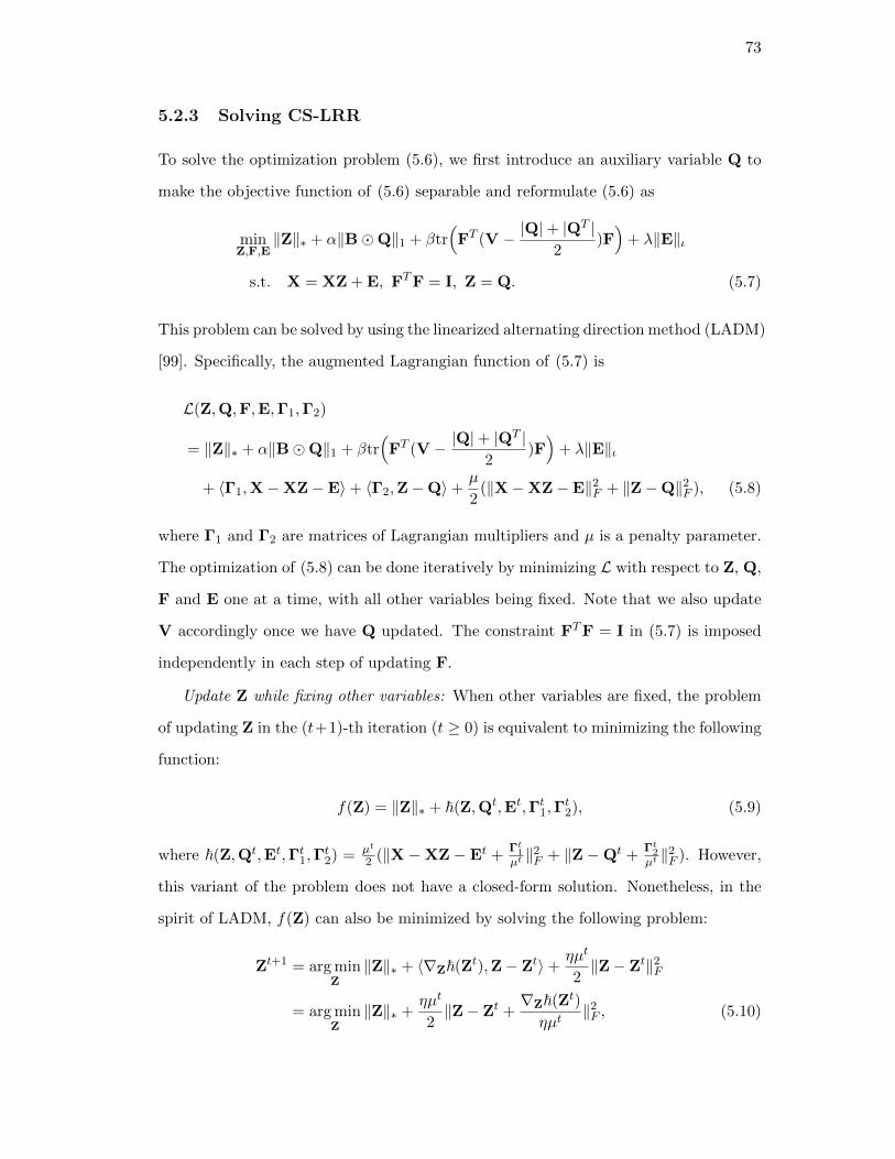
73
5.2.3 Solving CS-LRR
To solve the optimization problem (5.6), we first introduce an auxiliary variable Q to
make the objective function of (5.6) separable and reformulate (5.6) as
minZ,F,E
‖Z‖∗ + α‖BQ‖1 + βtr(FT (V − |Q|+ |Q
T |2
)F)
+ λ‖E‖ι
s.t. X = XZ + E, FTF = I, Z = Q. (5.7)
This problem can be solved by using the linearized alternating direction method (LADM)
[99]. Specifically, the augmented Lagrangian function of (5.7) is
L(Z,Q,F,E,Γ1,Γ2)
= ‖Z‖∗ + α‖BQ‖1 + βtr(FT (V − |Q|+ |Q
T |2
)F)
+ λ‖E‖ι
+ 〈Γ1,X−XZ−E〉+ 〈Γ2,Z−Q〉+µ
2(‖X−XZ−E‖2F + ‖Z−Q‖2F ), (5.8)
where Γ1 and Γ2 are matrices of Lagrangian multipliers and µ is a penalty parameter.
The optimization of (5.8) can be done iteratively by minimizing L with respect to Z, Q,
F and E one at a time, with all other variables being fixed. Note that we also update
V accordingly once we have Q updated. The constraint FTF = I in (5.7) is imposed
independently in each step of updating F.
Update Z while fixing other variables: When other variables are fixed, the problem
of updating Z in the (t+1)-th iteration (t ≥ 0) is equivalent to minimizing the following
function:
f(Z) = ‖Z‖∗ + ~(Z,Qt,Et,Γt1,Γt2), (5.9)
where ~(Z,Qt,Et,Γt1,Γt2) = µt
2 (‖X −XZ − Et +Γt1µt ‖
2F + ‖Z −Qt +
Γt2µt ‖
2F ). However,
this variant of the problem does not have a closed-form solution. Nonetheless, in the
spirit of LADM, f(Z) can also be minimized by solving the following problem:
Zt+1 = arg minZ
‖Z‖∗ + 〈∇Z~(Zt),Z− Zt〉+ηµt
2‖Z− Zt‖2F
= arg minZ
‖Z‖∗ +ηµt
2‖Z− Zt +
∇Z~(Zt)
ηµt‖2F , (5.10)

74
where ∇Z~ is the partial differential of ~ with respect to Z and η is a constant satisfying
η > ‖X‖2. For this problem, ∇Z~ = µtXT (XZ−X+Et− Γt1µt )+µt(Z−Qt+
Γt2µt ). Then
the closed-form solution for Z is given as
Zt+1 = Υ 1ηµt
(Zt − ∇Z~(Zt)
ηµt), (5.11)
where Υ(·) denotes singular value thresholding operator [100].
Update Q while fixing other variables: When other variables are fixed, the problem
of updating Q is
minQ
α‖BQ‖1 + βtr(
(Ft)T (V − |Q|+ |QT |
2)Ft)
+µt
2‖Q− (Zt+1 +
Γt2µt
)‖2F . (5.12)
According to (5.5), we have tr((Ft)T (V− |Q|+|QT |
2 )Ft) = ‖ΘtQ‖1, where θti,j = 12‖f
t,i−
f t,j‖22. Here, f t,i and f t,j denote the i-th and j-th row of the matrix Ft, respectively.
Therefore, (5.12) can be written as follows:
minQ
α‖(B +β
αΘt)Q‖1 +
µt
2‖Q− (Zt+1 +
Γt2µt
)‖2F , (5.13)
which has the following closed-form solution:
Qt+1 = T( αµt,B+ β
αΘt)
(Zt+1 +Γt2µt
), (5.14)
where the (i, j)-th entry of T(τ,H)(A) is given by Tτhi,j (ai,j) with Tτ ′(x) = max(x −
τ ′, 0)+min(x+τ ′, 0) [96]. After this, we update Vt+1 by setting ∀i, vt+1i,i =
∑j
|qt+1i,j |+|q
t+1j,i |
2 .
Update F while fixing other variables: When other variables are fixed, the problem
of updating F is
Ft+1 = arg minFTF=I
tr(FT (Vt+1 − |Qt+1|+ |(Qt+1)T |
2)F). (5.15)
Defining Mt+1 = Vt+1 − |Qt+1|+|(Qt+1)T |
2 , this problem has a closed-form solution that
involves eigendecomposition of Mt+1. In particular, the columns of Ft+1 are given by
the eigenvectors of Mt+1 associated with its smallest Lmax eigenvalues.
Update E while fixing other variables: When other variables are fixed, the problem
of updating E can be written as
Et+1 = arg minE
λ‖E‖ι +µt
2‖E−Ct+1‖2F , (5.16)
75
where Ct+1 = X−XZt+1+Γt1µt . For HOG features, we define Ei to be the approximation
error with respect to Xi (the matrix version of xi) and set the error term ‖E‖ι ≡∑Ni=1 ‖Ei‖2,1 to ensure robustness against “corruptions” in the orientation of each HOG
feature descriptor; this is because the background information is included in the feature
vector. Then (5.16) can be decomposed into N independent subproblems. In order to
update ei, we first convert the vector ct+1i to a matrix Ct+1
i ∈ Rnb×9 and then solve
the following problem:
Et+1i = arg min
Ei
λ‖Ei‖2,1 +µt
2‖Ei − Ct+1
i ‖2F , (5.17)
where Et+1i ∈ Rnb×9 is the reshaped “image” of the vector et+1
i . This problem can be
solved using [95, Lemma 3.2]. For MBH features, since the noise due to background
motion is eliminated, we simply set the error term ‖E‖ι ≡ ‖E‖2,1; then (5.16) can be
written as
Et+1 = arg minE
λ‖E‖2,1 +µt
2‖E−Ct+1‖2F , (5.18)
which can also be solved by using [95, Lemma 3.2]. The complete algorithm is outlined
in Algorithm 8.
5.3 Hierarchical Subspace Clustering Based on CS-LRR Model
We now introduce a hierarchical subspace clustering algorithm based on CS-LRR ap-
proach for learning action attributes at multiple levels of our UoS model and for au-
tomatically determining the final number of attributes present in a high-dimensional
dataset without prior knowledge. To begin, we introduce some notation used in this
section. We define πp|` to be the set containing the indexes of all xi’s that are assigned
to the `-th subspace at the p-th level (p ≥ 0) of the hierarchical structure, and let
Xp|` = [xi : i ∈ πp|`] ∈ Rm×Np|` be the corresponding set of signals, where Np|` is the
number of signals in Xp|`.2 Let Lp denote the number of subspaces at the p-th level,
then we have∑Lp
`=1Np|` = N and X =⋃Lp`=1 Xp|` for all p’s. The subspace underlying
2At level 0, we have only one cluster at the top, i.e., π0|1 = 1, 2, . . . , N, X0|1 = X and N0|1 = N .
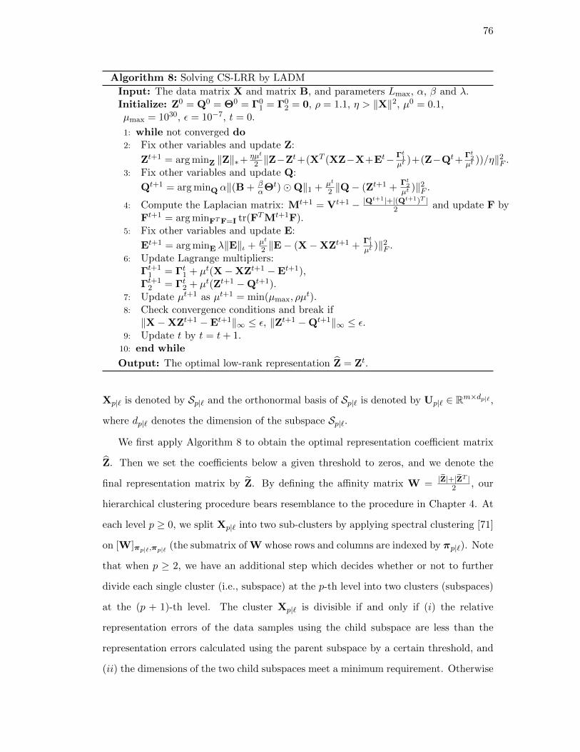
76
Algorithm 8: Solving CS-LRR by LADM
Input: The data matrix X and matrix B, and parameters Lmax, α, β and λ.Initialize: Z0 = Q0 = Θ0 = Γ0
1 = Γ02 = 0, ρ = 1.1, η > ‖X‖2, µ0 = 0.1,
µmax = 1030, ε = 10−7, t = 0.
1: while not converged do2: Fix other variables and update Z:
Zt+1 = arg minZ ‖Z‖∗+ηµt
2 ‖Z−Zt+(XT (XZ−X+Et− Γt1µt )+(Z−Qt+
Γt2µt ))/η‖2F .
3: Fix other variables and update Q:
Qt+1 = arg minQ α‖(B + βαΘt)Q‖1 + µt
2 ‖Q− (Zt+1 +Γt2µt )‖2F .
4: Compute the Laplacian matrix: Mt+1 = Vt+1 − |Qt+1|+|(Qt+1)T |
2 and update F byFt+1 = arg minFTF=I tr(FTMt+1F).
5: Fix other variables and update E:
Et+1 = arg minE λ‖E‖ι + µt
2 ‖E− (X−XZt+1 +Γt1µt )‖2F .
6: Update Lagrange multipliers:Γt+1
1 = Γt1 + µt(X−XZt+1 −Et+1),Γt+1
2 = Γt2 + µt(Zt+1 −Qt+1).7: Update µt+1 as µt+1 = min(µmax, ρµ
t).8: Check convergence conditions and break if‖X−XZt+1 −Et+1‖∞ ≤ ε, ‖Zt+1 −Qt+1‖∞ ≤ ε.
9: Update t by t = t+ 1.10: end while
Output: The optimal low-rank representation Z = Zt.
Xp|` is denoted by Sp|` and the orthonormal basis of Sp|` is denoted by Up|` ∈ Rm×dp|` ,
where dp|` denotes the dimension of the subspace Sp|`.
We first apply Algorithm 8 to obtain the optimal representation coefficient matrix
Z. Then we set the coefficients below a given threshold to zeros, and we denote the
final representation matrix by Z. By defining the affinity matrix W = |Z|+|ZT |2 , our
hierarchical clustering procedure bears resemblance to the procedure in Chapter 4. At
each level p ≥ 0, we split Xp|` into two sub-clusters by applying spectral clustering [71]
on [W]πp|`,πp|` (the submatrix of W whose rows and columns are indexed by πp|`). Note
that when p ≥ 2, we have an additional step which decides whether or not to further
divide each single cluster (i.e., subspace) at the p-th level into two clusters (subspaces)
at the (p + 1)-th level. The cluster Xp|` is divisible if and only if (i) the relative
representation errors of the data samples using the child subspace are less than the
representation errors calculated using the parent subspace by a certain threshold, and
(ii) the dimensions of the two child subspaces meet a minimum requirement. Otherwise

77
Algorithm 9: HCS-LRR (the p-th level, 2 ≤ p ≤ P − 1)
Input: The affinity matrix W obtained from Algorithm 8. A set of clustersXp|`
Lp`=1 with their corresponding indexes πp|`
Lp`=1, their underlying subspace
bases Up|`Lp`=1 and gp|`
Lp`=1, and parameters γ, % and dmin.
1: L = 0.2: for all ` = 1 to Lp do3: if gp|` = 1 then4: θ = 0.5: Apply spectral clustering on [W]πp|`,πp|` to split Xp|` into Xp|` = Σ1 ∪Σ2
(πp|` = χ1 ∪ χ2).6: ∀c = 1, 2, estimate dΣc and UΣc of SΣc using Σc.
7: ∀c = 1, 2, compute δc and ζc. If δc−ζcδc≥ %, θ = θ + 1.
8: if θ ≥ 1 and min(dΣ1 , dΣ2) ≥ dmin then9: ∀c = 1, 2, X
p+1|L+c= Σc, πp+1|L+c
= χc, Up+1|L+c
= UΣc , and gp+1|L+c
= 1.
10: L = L+ 2.11: else12: X
p+1|L+1= Xp|`, πp+1|L+1
= πp|`, Up+1|L+1
= Up|`, gp|` = 0, gp+1|L+1
= 0,
and L = L+ 1.13: end if14: else15: X
p+1|L+1= Xp|`, πp+1|L+1
= πp|`, Up+1|L+1
= Up|`, gp+1|L+1= 0, and
L = L+ 1.16: end if17: end for18: Lp+1 = L.
Output: A set of clusters Xp+1|`Lp+1
`=1 with their corresponding indexes
πp+1|`Lp+1
`=1 , orthonormal bases of the attributes Up+1|`Lp+1
`=1 and gp+1|`Lp+1
`=1 .
the cluster Xp|` is a leaf cluster and this cluster will not be divided any further. This
process is repeated until we reach a predefined maximum level in the hierarchy denoted
by P . The hierarchical subspace clustering algorithm based on CS-LRR model for any
level 2 ≤ p ≤ P − 1 is described in Algorithm 9, which we term HCS-LRR. It is worth
noting that the maximum number of leaf clusters is Lmax = 2P in this setting, which
we set as a key input parameter for Algorithm 8.
5.4 Attribute Visualization and Semantic Summarization
Given the learned subspaces at different levels of the hierarchical structure, our next
goal is to develop a method that helps an expert-in-the-loop to visualize the learned

78
human action attributes, give them semantic labels, and use the labeled attributes to
summarize long video sequences of human activities in terms of language at different
resolutions. As we have shown previously in Chapter 4, if frame-by-frame silhouette
features are used for learning the human action attributes, the attributes (subspaces)
can be easily visualized by reshaping the first few vectors of the orthonormal bases of
the subspaces into an image format and displaying the scaled versions of these images.
However, if other spatial or spatio-temporal features like HOG or MBH are used, the
attributes or the subspaces learned using HCS-LRR algorithm cannot be visualized
directly by just reshaping each dimension of the subspace in the feature domain.
5.4.1 Visualization of Attributes Using HOG Features
In the case of HOG features, inspired by HOGgles [101], we propose an algorithm
to visualize the learned attributes by mapping them back to the pixel domain. In
particular, we are interested in building a mapping between the pixel (image) space
and the HOG feature space and use this mapping to transform the bases of the HOG
feature subspaces into the image space and visualize the attributes. An algorithm
based on paired dictionary learning is used to develop this mapping. Concretely, let
XI = [xI1,xI2, . . . ,x
INp
] ∈ RmI×Np be the collection of Np vectorized patches of size
mI = nσ×nσ pixels from video frames, and XH = [xH1 ,xH2 , . . . ,x
HNp
] ∈ RmH×Np be the
corresponding HOG feature vectors of the patches in XI . Here, the dimensionality of
the HOG features of each patch mH depends on the choice of the number of bins in the
histogram. For better visualization quality, we extract 18-bin contrast specific HOG
features. Hence, mH = 18 in this work. Then, two dictionaries, i.e., overcomplete bases
whose columns span the data space, DI ∈ RmI×K and DH ∈ RmH×K consisting of K
atoms are learned to represent image space and HOG feature space, respectively, such
that the sparse representation of any xIi ∈ XI in terms of DI should be the same as
that of xHi ∈ XH in terms of DH . Similar to [102], paired dictionary learning problem
79
can be considered as solving the following optimization problem:
minDI ,DH ,αi
Npi=1
Np∑i=1
(‖xIi −DIαi‖22 + ‖xHi −DHαi‖22
)s.t. ‖αi‖1 ≤ ε,∀i, ‖dI,k‖2 ≤ 1, ‖dH,k‖2 ≤ 1,∀k, (5.19)
where αi denotes the sparse code with respect to xIi /xHi , and dI,k and dH,k denote the
k-th column of DI and DH , respectively.
Equation (5.19) can be simplified into a standard dictionary learning and sparse
coding problem and can be solved using the K-SVD algorithm [16]. Once we have the
collection of HOG feature vectors that lie on a subspace, we can find orthogonal basis of
the attribute (subspace) using eigenanalysis. However, these orthogonal basis vectors
are not guaranteed to be non-negative, which is the characteristic of HOG feature
vectors. Therefore, we use Non-negative Matrix Factorization (NMF) [103] to obtain
non-negative basis vectors (not necessarily orthogonal) of each subspace in the feature
domain. In order to obtain the corresponding pixel values of each of the basis vectors,
we split every basis vector into nb segments and each segment is of length mH (since
the entire basis vector is the concatenation of HOG features extracted from different
patches or blocks in a video frame). After this, we infer the sparse representation of
every small segment in the basis vector with respect to DH using Orthogonal Matching
Pursuit (OMP) [104], and use the resulting sparse code on DI to recover the pixel
values corresponding to that patch (which has mI values) in the frame. This procedure
is repeated for all the segments in the basis vector to obtain its image version for
visualization. Finally, the subspace can be labeled by visualizing the subspaces, similar
to what was done in the case of silhouette features.
5.4.2 Visualization of Attributes Using MBH Features
Unlike HOG features, it is not feasible to learn the mapping between the feature domain
and the pixel domain for MBH features because most of the patches in the pixel domain
will be mapped to zero in the MBH feature domain except the blocks in the action
interest region. Instead, we store an intermediate output, i.e., the magnitude of the
80
optical flow for visualization purpose. In other words, for every nτ consecutive optical
flow fields, we use the magnitude of the first optical flow field, which can be visualized
by an image, as the representative of all these nτ optical flow fields. Then for every nσ×
nσ × nτ spatio-temporal patch (block) of optical flow fields, from which MBH features
are extracted, we have one nσ×nσ optical flow (magnitude) patch associated with this
block. We use MBH features for clustering the data samples into different attributes.
Then, we use the optical flow frames corresponding to the data samples in each cluster
or attribute to visualize the subspace. The optical flow frames look very similar to the
silhouette features with non-zero elements present only in the location where there is
movement between the original video frames. Thus, the attributes (subspaces) can be
easily visualized by reshaping the first few columns of the orthonormal bases of the
subspaces, which are now represented by optical flow frames, into an image format.
5.5 Action Recognition Using Learned Subspaces
In this section, we describe the classification strategy to perform action recognition
using the hierarchical union of subspaces learned from Algorithm 9. We assume HCS-
LRR ends up with LP leaf subspaces and the orthonormal bases of these subspaces are
being represented by UP |` ∈ Rm×dP |`LP`=1. We begin our discussion for the classical
multi-class closed set recognition problem.
5.5.1 Closed Set Action Recognition Using k-NN
First, we develop a closed set action recognition method based on a k nearest neighbors
classifier. Let Φi ∈ Rm×ξiNTi=1 be a collection of NT labeled training samples, where
ξi denotes the number of feature vectors of the i-th training video sequence. Given
a test video sequence, whose feature vectors are denoted by Φ = [φ1, φ2, . . . , φξ], we
compute the distance between the feature vectors of every training and test sequence
as follows. Let Φ = [φ1,φ2, . . . ,φξ] be any training sample (we remove subscript
i for ease of notation), we first apply Dynamic Time Warping (DTW) [91] to align
the two action sequences using the HOG/MBH feature vectors and remove redundant
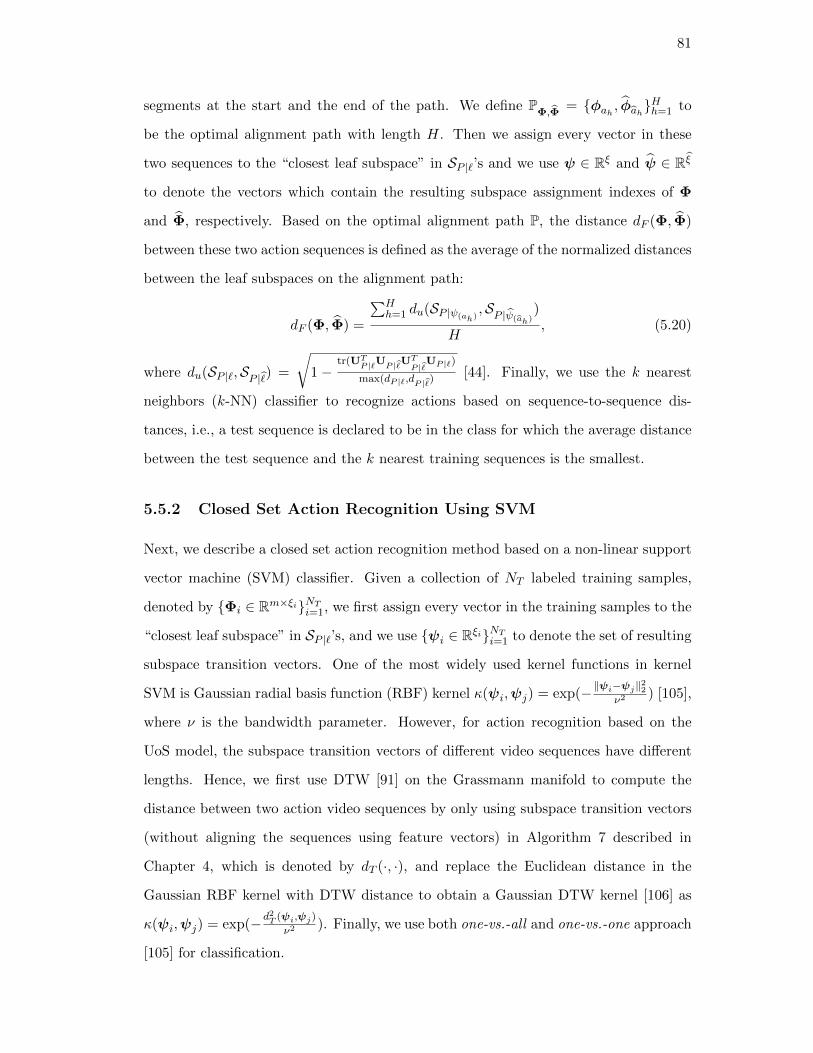
81
segments at the start and the end of the path. We define PΦ,Φ
= φah , φahHh=1 to
be the optimal alignment path with length H. Then we assign every vector in these
two sequences to the “closest leaf subspace” in SP |`’s and we use ψ ∈ Rξ and ψ ∈ Rξ
to denote the vectors which contain the resulting subspace assignment indexes of Φ
and Φ, respectively. Based on the optimal alignment path P, the distance dF (Φ, Φ)
between these two action sequences is defined as the average of the normalized distances
between the leaf subspaces on the alignment path:
dF (Φ, Φ) =
∑Hh=1 du(SP |ψ(ah)
,SP |ψ(ah)
)
H, (5.20)
where du(SP |`,SP |) =
√1−
tr(UTP |`UP |UT
P |UP |`)
max(dP |`,dP |) [44]. Finally, we use the k nearest
neighbors (k-NN) classifier to recognize actions based on sequence-to-sequence dis-
tances, i.e., a test sequence is declared to be in the class for which the average distance
between the test sequence and the k nearest training sequences is the smallest.
5.5.2 Closed Set Action Recognition Using SVM
Next, we describe a closed set action recognition method based on a non-linear support
vector machine (SVM) classifier. Given a collection of NT labeled training samples,
denoted by Φi ∈ Rm×ξiNTi=1, we first assign every vector in the training samples to the
“closest leaf subspace” in SP |`’s, and we use ψi ∈ RξiNTi=1 to denote the set of resulting
subspace transition vectors. One of the most widely used kernel functions in kernel
SVM is Gaussian radial basis function (RBF) kernel κ(ψi,ψj) = exp(−‖ψi−ψj‖22
ν2) [105],
where ν is the bandwidth parameter. However, for action recognition based on the
UoS model, the subspace transition vectors of different video sequences have different
lengths. Hence, we first use DTW [91] on the Grassmann manifold to compute the
distance between two action video sequences by only using subspace transition vectors
(without aligning the sequences using feature vectors) in Algorithm 7 described in
Chapter 4, which is denoted by dT (·, ·), and replace the Euclidean distance in the
Gaussian RBF kernel with DTW distance to obtain a Gaussian DTW kernel [106] as
κ(ψi,ψj) = exp(−d2T (ψi,ψj)
ν2). Finally, we use both one-vs.-all and one-vs.-one approach
[105] for classification.
82
5.5.3 Open Set Action Recognition
We now consider the open set action recognition problem, where we assume to have
knowledge of B known actions in the training stage while new or never-before-seen ac-
tions are also encountered in the test stage [107–109]. We first describe our approach for
the open set problem based on the k nearest neighbors classifier. Similar to the solution
for the traditional multi-class closed set recognition problem described in Section 5.5.1,
we first compute distances between every pair of the training video sequences in each
class using (5.20). Then for every training sequence, we calculate the average distance
between this training sequence and its k nearest neighbors within the same class, and
we use ϕs to denote the maximum of all the averaged distances associated with all the
training sequences in the s-th class (s = 1, 2, . . . ,B). For a test sequence, we first apply
k-NN to assign a “tentative” class membership for this sequence, which is denoted by
s, and we use ϕ to denote the average distance between this test sequence and its k
nearest training sequences in the s-th class. Finally, we declare this test sequence to
be in the s-th class if ϕ ≤ ϕsς, where ς > 1 is a predefined thresholding parameter,
otherwise it is labeled as a “new” action class.
Next, we discuss our solution for the open set problem based on one-vs.-all SVM.
We first train B one-vs.-all SVM classifiers using training sequences as proposed in
Section 5.5.2. Then for a test sequence, we declare it to be in the s-th class if (i)
the classifier associated with the s-th action returns the maximum score among all the
classifiers and (ii) this maximum score is above zero; otherwise, the test sequence is
declared to be a “new” action.
5.6 Experimental Results
We assess our proposed method on five human action datasets. Our first objective is to
visually interpret and label the learned action attributes from HCS-LRR and to inves-
tigate the utility of the multi-resolution action attributes in semantic summarization
of long video sequences of complex human activities. The second goal is to evaluate
the performance of the learned action attributes in human action recognition/open set
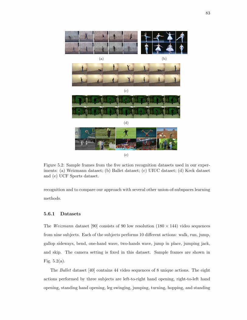
83
(a) (b)
(c)
(d)
(e)
Figure 5.2: Sample frames from the five action recognition datasets used in our exper-iments: (a) Weizmann dataset; (b) Ballet dataset; (c) UIUC dataset; (d) Keck datasetand (e) UCF Sports dataset.
recognition and to compare our approach with several other union-of-subspaces learning
methods.
5.6.1 Datasets
The Weizmann dataset [90] consists of 90 low resolution (180 × 144) video sequences
from nine subjects. Each of the subjects performs 10 different actions: walk, run, jump,
gallop sideways, bend, one-hand wave, two-hands wave, jump in place, jumping jack,
and skip. The camera setting is fixed in this dataset. Sample frames are shown in
Fig. 5.2(a).
The Ballet dataset [40] contains 44 video sequences of 8 unique actions. The eight
actions performed by three subjects are left-to-right hand opening, right-to-left hand
opening, standing hand opening, leg swinging, jumping, turning, hopping, and standing

84
still. Fig. 5.2(b) presents the sample frames of each action. Each video may contain
several actions in this dataset. In total, there are 59 video clips, each containing only
one action.
The UIUC dataset [110] consists of 532 videos corresponding to eight subjects. In
total, there are 14 action classes, including walking, running, jumping, waving, jumping
jacks, clapping, jump from situp, raise one hand, stretching out, turning, sitting to
standing, crawling, pushing up and standing to sitting (refer to Fig. 5.2(c)). In this
work, we use the last section of the dataset, which contains 70 action sequences of all
14 actions performed by only one person and each action is performed five times.
The Keck gesture dataset [92] is collected using a camera with 640×480 resolution. It
consists of 14 different gestures, including turn left, turn right, attention left, attention
right, flap, stop left, stop right, stop both, attention both, start, go back, close distance,
speed up, and come near. Example frames of this dataset are shown in Fig. 5.2(d). Each
of these 14 actions is performed by three people. In each video sequence, the subject
repeats the same gesture three times. Therefore the total number of video sequences
with static background is 14× 3× 3 = 126.
The UCF Sports dataset [111] contains 150 video samples, which are collected from
various broadcast television channels such as BBC and ESPN. There are 10 action
classes included in this dataset: diving, golf swing, kicking, lifting, horse riding, running,
skateboarding, swinging-bench, swinging-side and walking, as shown in Fig. 5.2(e). In
this work, we exclude the videos belonging to horse riding and skateboarding actions
as there is little to no body movement in these two classes. We also exclude two videos
in the diving action since there are two subjects in each of those videos. This leaves us
with 124 video sequences of 8 actions.
5.6.2 Semantic Labeling and Summarization
In this section, we study the performance of HCS-LRR using HOG/MBH features for
semantic summarization of multiple actions in a long video sequence. We compare the
performance of HCS-LRR with several state-of-the-art subspace clustering algorithms
such as Low-Rank Representation (LRR) [42], Sparse Subspace Clustering (SSC) [13],

85
(a)Stand/Clapping
(b) Knee bend (c)Wave/Jumping
jack
(d) Stretching
out/Stand with
one hand up
(e) Upper posi-
tion of push up
(f) Lower posi-
tion of push up
(g)Stand/Clapping
(h) Knee bend (i) Jumping
jack/Stand with
two hands out
(j) Wave
(k) Stand with
one hand up
(l) Stretching
out/Stand with
two hands up
(m) Upper posi-
tion of push up
(n) Lower posi-
tion of push up
(o)Stand/Clapping
(p) Lower posi-
tion of push up
(q) Knee bend (r) Jumpingjack
(s) Upper posi-
tion of push up
(t) Wave
(u) Stand
with one hand
up/Stand
(v)Wave/Jumping
jack
Figure 5.3: Visualization and interpretation of attributes learned using the frames fromUIUC dataset. (a)-(f) represent the subspaces at the 3rd level of HCS-LRR. (g)-(n)represent the leaf subspaces (4th level) learned by HCS-LRR. (o)-(v) represent thesubspaces which are learned using SC-LRR.
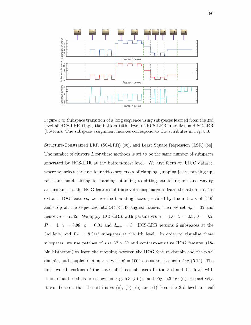
86
Frame indexesabcdef
Su
bsp
ace
in
de
xe
s
Frame indexesghij
kl
mn
Su
bsp
ace
in
de
xe
s
Frame indexesopqrst
uv
Su
bsp
ace
in
de
xe
s
Figure 5.4: Subspace transition of a long sequence using subspaces learned from the 3rdlevel of HCS-LRR (top), the bottom (4th) level of HCS-LRR (middle), and SC-LRR(bottom). The subspace assignment indexes correspond to the attributes in Fig. 5.3.
Structure-Constrained LRR (SC-LRR) [96], and Least Square Regression (LSR) [86].
The number of clusters L for these methods is set to be the same number of subspaces
generated by HCS-LRR at the bottom-most level. We first focus on UIUC dataset,
where we select the first four video sequences of clapping, jumping jacks, pushing up,
raise one hand, sitting to standing, standing to sitting, stretching out and waving
actions and use the HOG features of these video sequences to learn the attributes. To
extract HOG features, we use the bounding boxes provided by the authors of [110]
and crop all the sequences into 544 × 448 aligned frames; then we set nσ = 32 and
hence m = 2142. We apply HCS-LRR with parameters α = 1.6, β = 0.5, λ = 0.5,
P = 4, γ = 0.98, % = 0.01 and dmin = 3. HCS-LRR returns 6 subspaces at the
3rd level and LP = 8 leaf subspaces at the 4th level. In order to visualize these
subspaces, we use patches of size 32 × 32 and contrast-sensitive HOG features (18-
bin histogram) to learn the mapping between the HOG feature domain and the pixel
domain, and coupled dictionaries with K = 1000 atoms are learned using (5.19). The
first two dimensions of the bases of those subspaces in the 3rd and 4th level with
their semantic labels are shown in Fig. 5.3 (a)-(f) and Fig. 5.3 (g)-(n), respectively.
It can be seen that the attributes (a), (b), (e) and (f) from the 3rd level are leaf

87
nodes and hence, translate as they were to the 4th level. However, the attribute (c)
corresponding to Wave/Jumping jack at the 3rd level is further divided into attributes
(i) and (j) corresponding to Jumping jack/Stand with two hands out and One-hand wave
at the 4th level, respectively. Similarly, the attribute (d) corresponding to Stretching
out/Stand with one hand up at the 3rd level is further divided into attributes (k) and
(l) corresponding to Stand with one hand up and Stretching out/Stand with two hands
up in the bottom level, respectively. To demonstrate semantic summarization using
these learned attributes on a complex human activity, we select the last video sequence
of each of the aforementioned eight actions as the test sequences and create a long video
stream by concatenating these sequences. The semantic summary is illustrated as the
subspace transition of the frames in Fig. 5.4, where different actions in the sequence are
delimited by green lines. One can summarize the actions in terms of natural language by
using the attribute assignment indexes and the corresponding labels. We compare HCS-
LRR with other subspace clustering algorithms in terms of action recognition of the test
sequences by setting L = 8 for other approaches. SC-LRR also gives perfect recognition
accuracy based on k-NN classifier. To compare SC-LRR with our technique in terms
of semantic summarization, we apply SC-LRR on the training sequences to learn 8
attributes, and the corresponding labeled subspaces are illustrated in Fig. 5.3 (o)-(v).
However, compared to the attributes at the bottom level of HCS-LRR, we observe
that each of the attributes (u) and (v) learned using SC-LRR can have two totally
different interpretations. For instance, attribute (v) is a mixture of “one-hand wave”
and “jumping jack” action attributes. There are two advantages of using HCS-LRR
model over other techniques. First, the semantic summary of the video sequence can be
generated at different resolutions using attributes at different levels of the hierarchical
structure. Second, the summary generated using the attributes learned from HCS-LRR
is very clear because the actions are well-clustered into different attributes, but it is
difficult to generate a summary using the attributes learned from SC-LRR alone due
to confusion in the last two attributes. We provide the evidence of these advantages
in Fig. 5.4. In short, the semantic interpretation performance using HCS-LRR seems
better compared to SC-LRR.
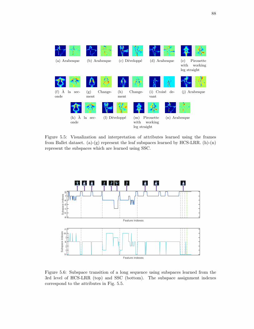
88
(a) Arabesque (b) Arabesque (c) Developpe (d) Arabesque (e) Pirouettewith workingleg straight
(f) A la sec-onde
(g) Change-ment
(h) Change-ment
(i) Croise de-vant
(j) Arabesque
(k) A la sec-onde
(l) Developpe (m) Pirouettewith workingleg straight
(n) Arabesque
Figure 5.5: Visualization and interpretation of attributes learned using the framesfrom Ballet dataset. (a)-(g) represent the leaf subspaces learned by HCS-LRR. (h)-(n)represent the subspaces which are learned using SSC.
Feature indexesa
b
c
d
e
f
g
Su
bsp
ace
in
de
xe
s
Feature indexesh
i
j
k
l
m
n
Su
bsp
ace
in
de
xe
s
Figure 5.6: Subspace transition of a long sequence using subspaces learned from the3rd level of HCS-LRR (top) and SSC (bottom). The subspace assignment indexescorrespond to the attributes in Fig. 5.5.

89
As another example, we experiment with Ballet dataset, where we select video clips
from standing hand opening, turning, hopping and standing still actions for learning
the attributes, with the number of sequences set to be 5, 5, 2 and 6, respectively.
We crop all the video frames into 288 × 288 pixels and extract MBH descriptors with
nσ = 32 and nτ = 3; thus m = 1458. Then we implement HCS-LRR with parameters
α = 0.8, β = 0.5, λ = 0.4, P = 3, γ = 0.98, % = 0.05 and dmin = 3. It has LP = 7
leaf subspaces at the 3rd level, and the first two basis vectors of each leaf subspace are
illustrated in Fig. 5.5 (a)-(g). Optical flow frames are used for visualization as explained
in Section 5.4.2. For testing purpose, we again choose the video clips belonging to the
aforementioned actions, with the number of clips set to be 2, 2, 1 and 4, respectively.
For these 9 test sequences from these four different actions, attributes learned using
SSC with L = 7 give perfect (100%) action recognition performance when using k-NN
classifier. The subspaces learned using SSC are shown in Fig. 5.5 (h)-(n). We again
concatenate all the test video clips to create a long video sequence and visualize the
subspace transition of the MBH features of the long sequence in Fig. 5.6. In the case
of HCS-LRR, it can be observed that the attribute (b) does not provide any additional
information than that is being provided by attribute (a). The attribute (i) learned using
SSC is not seen among the attributes at the bottom level of HCS-LRR. In addition,
there are no features of the test sequence that get assigned to attributes (a), (b) and
(n) due to the significant intraclass variations. In other words, SSC seems to offer
better summarization performance than HCS-LRR. However, the caveat here is that
in practice, the number of subspaces or attributes is not known a priori for SSC, while
HCS-LRR algorithm can automatically give an estimate of L.
5.6.3 Action Recognition
To quantify the discriminative power of the subspaces learned from HCS-LRR, we also
perform human action recognition using the action attributes learned by our proposed
method. We again compare the performance of HCS-LRR with LRR [42], SSC [13], SC-
LRR [96], and LSR [86]. Different from the experiments in Section 5.6.2, the number of
clusters L for these algorithms is now set (i) to be the same number of leaf subspaces

90
generated by HCS-LRR (which is denoted by 〈Algorithm〉-LP ) and (ii) to be the same
as the number of actions in the training data (which is denoted by 〈Algorithm〉-B).
For all these methods, including HCS-LRR, we first tune the parameters for clustering
to achieve their best recognition performance based on k-NN classifier. Once the at-
tributes are learned using these parameters, we further tune the parameters for SVM
classifiers to obtain their best recognition performance. We simply fix γ = 0.98 for all
the experiments. It should be noted that “SVM/ova” and “SVM/ovo” in Table 5.1
stand for “one-vs.-all SVM” and “one-vs.-one SVM,” respectively.
Closed Set Recognition
In this subsection, we carry out the closed set action recognition experiments on the five
datasets described in Section 5.6.1. We begin our experiments on Weizmann dataset,
where we use both HOG and MBH features to learn the attributes and evaluate all the
subspace/attribute learning approaches based on a leave-one-subject-out experiment.
We crop all the sequences into 88× 64 aligned frames and HOG features are extracted
with blocks of size nσ = 8, resulting in m = 792. Then we perform HCS-LRR with
parameters α = 1.2, β = 0.8, λ = 0.8, P = 5, % = 0.01 and dmin = 5, in which
setting it returns LP = 24 leaf subspaces for final attributes. As shown in Table 5.1,
our method significantly outperforms other subspace clustering approaches for all the
classifiers. To be specific, the lowest error is achieved by HCS-LRR when used with
one-vs.-one SVM classifier and the resulting recognition accuracy is 95.56%. Similarly,
we crop all the optical flow fields into 88 × 64 images and extract MBH features with
nσ = 8 and nτ = 3; hence m = 1584. We apply HCS-LRR with parameters α = 0.4,
β = 0.7, λ = 0.4, P = 5, % = 0.01 and dmin = 12, obtaining LP = 23 final subspaces.
We can see from Table 5.1 that for a fixed classifier, the recognition accuracy of all the
approaches is close to each other for 23 clusters. Our algorithm achieves the highest
classification accuracy among all the methods for k-NN classifier and one-vs.-all SVM
classifier. When using one-vs.-one SVM classifier, LRR-LP outperforms others and
HCS-LRR is only 2.2% (corresponds to 2 samples) behind LRR-LP . The main reason
for k-NN classifier outperforming SVM classifiers is that the original feature vectors

91
are used for aligning the training and test sequences in the case of k-NN classification,
and one can get perfect alignment of the video sequences using MBH features on clean
datasets such as Weizmann dataset. However, the SVM classifiers only use subspace
transition vectors instead of using the original feature vectors for alignment of the
sequences via the DTW kernel, which may degrade the recognition performance.

92
Tab
le5.
1:C
lose
dS
etA
ctio
nR
ecog
nit
ion
Res
ult
s(%
)
Dat
aset
Fea
ture
Cla
ssifi
erS
ub
spac
ecl
ust
erin
gm
eth
od
HC
S-L
RR
LR
R-LP
LR
R-B
SS
C-LP
SS
C-B
SC
-LR
R-LP
SC
-LR
R-B
LS
R-LP
LS
R-B
Wei
zman
n
HO
Gk-N
N90.0
073
.33
67.7
858
.89
52.2
276
.67
66.6
767.7
867.7
8S
VM
/ova
92.2
265
.56
52.2
258
.89
48.8
964
.44
63.3
358.8
965.5
6S
VM
/ovo
95.5
682
.22
66.6
764
.44
51.1
168
.89
68.8
971.1
172.2
2
MB
Hk-N
N91.1
188
.89
66.6
786
.67
65.5
690
.00
72.2
290.0
073.3
3S
VM
/ova
87.7
885
.56
64.4
485
.56
64.4
481
.11
68.8
986.6
771.1
1S
VM
/ovo
85.5
687.7
866
.67
84.4
461
.11
81.1
166.6
785.5
671.1
1
Bal
let
HO
Gk-N
N71.1
954
.24
32.2
052
.54
38.9
845
.76
49.1
540.6
845.7
6S
VM
/ova
67.8
059
.32
30.5
167.8
038
.98
66.1
042.3
754.2
461.0
2S
VM
/ovo
62.7
162
.71
52.5
464.4
142
.37
64.4
157.6
354.2
461.0
2
MB
Hk-N
N69.4
961
.02
54.2
457
.63
50.8
557
.63
54.2
461.0
252.5
4S
VM
/ova
71.1
969
.49
61.0
254
.24
20.3
461
.02
62.7
167.8
067.8
0S
VM
/ovo
69.4
967
.80
61.0
245
.76
44.0
767
.80
61.0
262.7
167.8
0
UIU
C
HO
Gk-N
N100
94.2
998
.57
98.5
785
.71
100
95.7
198.5
795.7
1S
VM
/ova
100
77.1
491
.43
98.5
781
.43
100
90.0
0100
91.4
3S
VM
/ovo
100
92.8
698
.57
100
78.5
7100
91.4
3100
85.7
1
MB
Hk-N
N100
100
98.5
7100
98.5
7100
82.8
6100
98.5
7S
VM
/ova
100
100
95.7
1100
100
100
78.5
7100
100
SV
M/o
vo100
100
95.7
1100
100
100
77.1
4100
100
Kec
kM
BH
k-N
N88.1
083
.33
78.5
779
.37
83.3
380
.16
80.9
576.1
970.6
3S
VM
/ova
87.3
076
.98
66.6
774
.60
71.4
379
.37
80.1
657.1
461.1
1S
VM
/ovo
90.4
876
.98
74.6
078
.57
73.8
184
.92
84.1
370.6
369.0
5
UC
FM
BH
k-N
N57.2
650
.81
47.5
856
.45
47.5
845
.97
38.7
155.6
543.5
5S
VM
/ova
66.1
367.7
460
.48
66.1
354
.84
64.5
250.8
164.5
254.0
3S
VM
/ovo
75.8
175
.00
57.2
675.8
153
.23
73.3
945.1
668.5
550.0
0

93
For Ballet dataset, we crop all the video frames into 288 × 288 pixels and extract
HOG descriptor of every frame with nσ = 32; hence m = 729. Since there is no
significant motion between consecutive frames, instead of using HOG features of each
frame separately, we take the sum of the HOG features of two adjacent frames at a
time and the sum is used as the feature of two adjacent frames. We perform HCS-LRR
with parameters α = 1.5, β = 0.2, λ = 2.2, P = 4, % = 0.05 and dmin = 3. The
number of subspaces returned by HCS-LRR at the finest scale is LP = 11. We evaluate
the subspace learning approaches using the leave-one-sequence-out scheme. The results
presented in Table 5.1 show that the proposed algorithm generates the lowest error
rates for k-NN and one-vs.-all SVM classifiers. Both SSC-LP and SC-LRR-LP perform
the best for one-vs.-one SVM classifier, and our method is only 1 sample lower than
these two approaches. After extracting the MBH descriptors with the same parameters
as in Section 5.6.2, we set α = 0.6, β = 0.2, λ = 0.2, P = 4, % = 0.05 and dmin = 3 for
HCS-LRR, which gives us LP = 9 leaf subspaces. The results are listed in Table 5.1,
from which we make the conclusion that by representing the human actions using the
attributes learned by HCS-LRR, we are able to recognize the actions at a superior rate
compared to other techniques.
Next, we evaluate our approach on UIUC dataset, where we again use both HOG
and MBH features and conduct leave-one-sequence-out experiments. To extract HOG
features, we crop all the sequences into 544×448 aligned frames by using the bounding
boxes provided by the authors of [110], and follow the same parameter setting as in
Section 5.6.2. We perform HCS-LRR with parameters α = 1, β = 0.2, λ = 0.1, P = 5,
% = 0.01 and dmin = 3, in which case it returns LP = 18 leaf subspaces. We crop all the
optical flow fields and the action interest region also has 544 × 448 pixels, then MBH
features are extracted with nσ = 32 and nτ = 2; therefore m = 4284 in this setting. We
set α = 0.2, β = 0.1, λ = 0.1, P = 5, % = 0.01 and dmin = 5 for HCS-LRR and finally
there are LP = 26 subspaces at the bottom-most level. The recognition accuracy for
all the methods is reported in Table 5.1. As Table 5.1 shows, both our method and
SC-LRR-LP obtain 100% recognition accuracy for both HOG and MBH features. In
general, using the number of clusters that is automatically generated from HCS-LRR

94
will improve the performance for almost all the methods.
To evaluate different methods on Keck dataset, we employ the leave-one-person-out
cross validation protocol. We only use MBH features to learn the attributes on this
dataset since the background of the aligned sequences is dynamic. We crop all the
optical flow fields into 288 × 288 images and extract MBH features with nσ = 32 and
nτ = 3, thereby resulting in m = 1458. We implement HCS-LRR with parameters
α = 0.1, β = 0.1, λ = 0.2, P = 5, % = 0.01 and dmin = 5. The number of leaf attributes
returned by HCS-LRR is LP = 28. The classification results are summarized in Ta-
ble 5.1. Our approach shows noticeable improvement in accuracy compared to other
state-of-the-art subspace clustering algorithms. The recognition rate reaches 90.48% for
HCS-LRR coupled with one-vs.-one SVM classifier, which outperforms SC-LRR-LP , the
second best, by 5.5%.
Finally, we examine the performance of different methods on UCF Sports dataset.
We align the sequences by applying the method proposed in [112] and subtract the
background using the approach described in [113], then we use the bounding boxes
provided by the authors of [111] to crop all the sequences and reshape them into 416×256
frames. Due to the dynamic property of the background, we again only use MBH
features to learn the attributes, where the MBH features are extracted with nσ = 32
and nτ = 3; so that m = 1872. We investigate the performance of the subspace
clustering approaches via the leave-one-sequence-out scheme. We use the following
parameters for HCS-LRR: α = 1.2, β = 0.1, λ = 0.3, P = 5, % = 0.005 and dmin = 3.
Finally, the output LP from HCS-LRR is 26 in this setting. Table 5.1 presents the
recognition results for all the methods. For k-NN classifier, our algorithm achieves the
highest classification accuracy, with 1 sample higher than the second best, SSC-LP .
The classification performance improves drastically when using SVM classifiers. For
one-vs.-one SVM classifier, both HCS-LRR and SSC-LP achieve 75.81% classification
accuracy, but HCS-LRR method has an additional advantage that it can generate the
number of clusters automatically without any prior knowledge of the data.

95
Table 5.2: Open Set Action Recognition Results (%)Dataset Classifier Subspace clustering method
UIUC
k-NN
HCS-LRR LRR-LP LRR-B SSC-LP SSC-B100 90.91 86.36 90.91 86.36
SC-LRR-LP SC-LRR-B LSR-LP LSR-B95.45 95.45 90.91 86.36
one-vs.-all SVM
HCS-LRR LRR-LP LRR-B SSC-LP SSC-B100 95.45 90.91 90.91 90.91
SC-LRR-LP SC-LRR-B LSR-LP LSR-B100 86.36 95.45 90.91
Keck
k-NN
HCS-LRR LRR-LP LRR-B SSC-LP SSC-B89.58 79.17 77.08 79.17 75.00
SC-LRR-LP SC-LRR-B LSR-LP LSR-B72.92 81.25 77.08 75.00
one-vs.-all SVM
HCS-LRR LRR-LP LRR-B SSC-LP SSC-B89.58 83.33 85.42 79.17 77.08
SC-LRR-LP SC-LRR-B LSR-LP LSR-B85.42 87.50 81.25 81.25
Open Set Recognition
One important advantage of learning human action attributes instead of representing
an entire action as a single feature vector is that an action that is absent in the training
stage can be identified as a new action class if it can be represented by the attributes
learned from other actions in the training data. Here, we show the effectiveness of
HCS-LRR for the open set action recognition problem. Consider a collection of Nk test
samples from B known classes and Nu test samples from U unknown classes, which are
denoted by (Φi, ϑi)Nk+Nui=1 , where ϑi ∈ 1, 2, . . . ,B for i ≤ Nk and ϑi = new for
i > Nk. We can measure the performance of our algorithm under the classification rule
C as εo =∑Nk+Nui=1 [C(Φi)=ϑi]
Nk+Nu.
UIUC dataset is used for the first set of experiments. From the 70 sequences in
the dataset, we select the first four video sequences of all classes except “walking” and
“standing to sitting” actions for training and the remaining 22 sequences for testing;
thus B = 12, U = 2, Nk = 12 and Nu = 10. We extract HOG features of the training
sequences as in Section 5.6.3 and perform HCS-LRR with parameters α = 0.8, β = 0.1,
λ = 0.4, P = 5, % = 0.01 and dmin = 3, which in turn provides us with LP = 19 leaf
subspaces. We can observe from Table 5.2 that HCS-LRR achieves perfect accuracy for
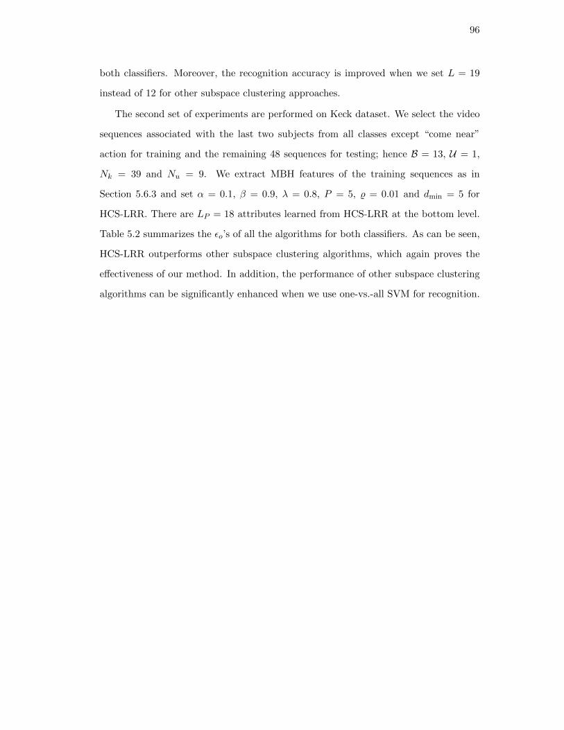
96
both classifiers. Moreover, the recognition accuracy is improved when we set L = 19
instead of 12 for other subspace clustering approaches.
The second set of experiments are performed on Keck dataset. We select the video
sequences associated with the last two subjects from all classes except “come near”
action for training and the remaining 48 sequences for testing; hence B = 13, U = 1,
Nk = 39 and Nu = 9. We extract MBH features of the training sequences as in
Section 5.6.3 and set α = 0.1, β = 0.9, λ = 0.8, P = 5, % = 0.01 and dmin = 5 for
HCS-LRR. There are LP = 18 attributes learned from HCS-LRR at the bottom level.
Table 5.2 summarizes the εo’s of all the algorithms for both classifiers. As can be seen,
HCS-LRR outperforms other subspace clustering algorithms, which again proves the
effectiveness of our method. In addition, the performance of other subspace clustering
algorithms can be significantly enhanced when we use one-vs.-all SVM for recognition.

97
Chapter 6
Conclusion and Future Work
In this thesis, we considered the problem of learning the geometric structure of high-
dimensional data. We proposed novel geometric models and algorithms based on the
union-of-subspaces model to learn the geometry efficiently.
In the first part of the thesis, we proposed a novel extension of the canonical union-of-
subspaces model, termed the metric-constrained union-of-subspaces (MC-UoS) model.
We first proposed several efficient iterative approaches for learning of an MC-UoS in
the ambient space using both complete and missing data. Moreover, these methods
were extended to the case of a higher-dimensional feature space such that one can deal
with MC-UoS learning problem in the feature space using complete and missing data.
Experiments on both synthetic and real data showed the effectiveness of our algorithms
and their superiority over the state-of-the-art union-of-subspaces learning algorithms.
Our future work includes estimation of the number and dimension of the subspaces
from the training data for MC-UoS learning in the feature space.
In the second part of the thesis, we put forth different models for learning the
human action attributes from video data based on UoS model. We first proposed
Hierarchical Sparse Subspace Clustering (HSSC) to learn the attributes, which does
not need the number of clusters to be specified and does not require labeled training
data to learn human action attributes, while avoiding generation of trivial attributes.
Then we proposed an extension of the canonical low-rank representation (LRR), termed
the clustering-aware structure-constrained low-rank representation (CS-LRR) model,
for unsupervised data-driven human action attribute learning. The proposed CS-LRR
model incorporates spectral clustering into the learning framework, which helps spectral
clustering achieve the best clustering results. Moreover, we introduced a hierarchical

98
subspace clustering approach based on CS-LRR model, called HCS-LRR model, which
again does not need the number of clusters to be specified a priori. Experimental
results on real video datasets showed the effectiveness of our clustering approach and
its superiority over the state-of-the-art union-of-subspaces learning algorithms for its
utility in semantic summarization of complex human activities at multiple resolutions as
well as human action recognition. One of the interesting avenues of future work involves
the development of a robust, spatio-temporal hierarchical tensor-UoS framework for
learning of semantically interpretable human action attributes and recognition of human
activities from multimodal video data.
99
References
[1] H. Hotelling, “Analysis of a complex of statistical variables into principal compo-nents,” J. Educ. Psych., vol. 24, pp. 417–441, 498–520, 1933.
[2] T. F. Cox and M. A. A. Cox, Multidimensional scaling. Chapman & Hall, 2000.
[3] S. T. Roweis and L. K. Saul, “Nonlinear dimensionality reduction by locally linearembedding,” Science, vol. 290, pp. 2323–2326, 2000.
[4] M. Elad, R. Goldenberg, and R. Kimmel, “Low bit-rate compression of facialimages,” IEEE Trans. Image Process., vol. 16, no. 9, pp. 2379–2383, 2007.
[5] R. G. Baraniuk, V. Cevher, and M. B. Wakin, “Low-dimensional models fordimensionality reduction and signal recovery: A geometric perspective,” Proc.IEEE, vol. 98, no. 6, pp. 959–971, 2010.
[6] S. Mika, B. Scholkopf, A. J. Smola, K.-R. Muller, M. Scholz, and G. Ratsch,“Kernel PCA and de-noising in feature spaces,” in Proc. Adv. Neural Inf. Process.Syst. (NIPS), 1998, pp. 536–542.
[7] M. Elad and M. Aharon, “Image denoising via sparse and redundant representa-tions over learned dictionaries,” IEEE Trans. Image Process., vol. 15, no. 12, pp.3736–3745, 2006.
[8] M. A. Turk and A. P. Pentland, “Face recognition using eigenfaces,” in Proc.IEEE Conf. Comput. Vis. Pattern Recognit. (CVPR), 1991, pp. 586–591.
[9] D. L. Swets and J. Weng, “Using discriminant eigenfeatures for image retrieval,”IEEE Trans. Pattern Anal. Mach. Intell., vol. 18, no. 8, pp. 831–836, 1996.
[10] J. Wright, A. Y. Yang, A. Ganesh, S. S. Sastry, and Y. Ma, “Robust face recogni-tion via sparse representation,” IEEE Trans. Pattern Anal. Mach. Intell., vol. 31,no. 2, pp. 210–227, 2009.
[11] J. Mairal, F. Bach, and J. Ponce, “Task-driven dictionary learning,” IEEE Trans.Pattern Anal. Mach. Intell., vol. 34, no. 4, pp. 791–804, 2012.
[12] S. Rao, R. Tron, R. Vidal, and Y. Ma, “Motion segmentation in the presenceof outlying, incomplete, or corrupted trajectories,” IEEE Trans. Pattern Anal.Mach. Intell., vol. 32, no. 10, pp. 1832–1845, 2010.
[13] E. Elhamifar and R. Vidal, “Sparse subspace clustering: Algorithm, theory, andapplications,” IEEE Trans. Pattern Anal. Mach. Intell., vol. 35, no. 11, pp. 2765–2781, 2013.
[14] H. H. Harman, Modern factor analysis. University of Chicago Press, 1976.
100
[15] B. Scholkopf, A. J. Smola, and K.-R. Muller, “Nonlinear component analysis as akernel eigenvalue problem,” Neural Comput., vol. 10, no. 5, pp. 1299–1319, 1998.
[16] M. Aharon, M. Elad, and A. Bruckstein, “K-SVD: An algorithm for designingovercomplete dictionaries for sparse representation,” IEEE Trans. Signal Process.,vol. 54, no. 11, pp. 4311–4322, 2006.
[17] Y. C. Eldar and M. Mishali, “Robust recovery of signals from a structured unionof subspaces,” IEEE Trans. Inf. Theory, vol. 55, no. 11, pp. 5302–5316, 2009.
[18] M. W. Marcellin, M. J. Gormish, A. Bilgin, and M. P. Boliek, “An overview ofJPEG-2000,” in Proc. IEEE Data Compression Conf. (DCC), 2000, pp. 523–541.
[19] J.-L. Starck, E. J. Candes, and D. L. Donoho, “The curvelet transform for imagedenoising,” IEEE Trans. Image Process., vol. 11, no. 6, pp. 670–684, 2002.
[20] T. Zhang, A. Szlam, and G. Lerman, “Median K-flats for hybrid linear modelingwith many outliers,” in Proc. IEEE Int. Conf. Comput. Vis. Workshops, 2009,pp. 234–241.
[21] B. V. Gowreesunker and A. H. Tewfik, “Learning sparse representation usingiterative subspace identification,” IEEE Trans. Signal Process., vol. 58, no. 6, pp.3055–3065, 2010.
[22] L. Balzano, A. Szlam, B. Recht, and R. Nowak, “K-subspaces with missing data,”in Proc. IEEE Statistical Signal Processing Workshop (SSP), 2012, pp. 612–615.
[23] W. Hong, J. Wright, K. Huang, and Y. Ma, “Multiscale hybrid linear modelsfor lossy image representation,” IEEE Trans. Image Process., vol. 15, no. 12, pp.3655–3671, 2006.
[24] K. Pearson, “On lines and planes of closest fit to systems of points in space,”Philos. Mag., vol. 2, no. 6, pp. 559–572, 1901.
[25] K. Fukunaga, Introduction to statistical pattern recognition. Academic Press,1990.
[26] B. Scholkopf, A. J. Smola, and K.-R. Muller, “Kernel principal component anal-ysis,” Advances in kernel methods: support vector learning, pp. 327–352, 1999.
[27] M. Belkin and P. Niyogi, “Laplacian eigenmaps for dimensionality reduction anddata representation,” Neural Comput., vol. 15, no. 6, pp. 1373–1396, 2003.
[28] J. Ham, D. D. Lee, S. Mika, and B. Scholkopf, “A kernel view of the dimensionalityreduction of manifolds,” in Proc. Int. Conf. Mach. Learn. (ICML), 2004, pp. 47–54.
[29] R. Vidal, Y. Ma, and S. Sastry, “Generalized principal component analysis(GPCA),” IEEE Trans. Pattern Anal. Mach. Intell., vol. 27, no. 12, pp. 1945–1959, 2005.
[30] L. Zelnik-Manor, K. Rosenblum, and Y. C. Eldar, “Dictionary optimization forblock-sparse representations,” IEEE Trans. Signal Process., vol. 60, no. 5, pp.2386–2395, 2012.

101
[31] M. Soltanolkotabi and E. J. Candes, “A geometric analysis of subspace clusteringwith outliers,” Ann. Stat., vol. 40, no. 4, pp. 2195–2238, 2012.
[32] E. L. Dyer, A. C. Sankaranarayanan, and R. G. Baraniuk, “Greedy feature se-lection for subspace clustering,” J. Mach. Learn. Res., vol. 14, pp. 2487–2517,2013.
[33] R. Heckel and H. Bolcskei, “Robust subspace clustering via thresholding,”arXiv:1307.4891, 2013.
[34] M. Soltanolkotabi, E. Elhamifar, and E. J. Candes, “Robust subspace clustering,”Ann. Stat., vol. 42, no. 2, pp. 669–699, 2014.
[35] T. Zhang, A. Szlam, Y. Wang, and G. Lerman, “Hybrid linear modeling via localbest-fit flats,” Int. J. Comput. Vis., vol. 100, no. 3, pp. 217–240, 2012.
[36] Z. Ghahramani and G. E. Hinton, “The EM algorithm for mixtures of factoranalyzers,” CRG-TR-96-1, University of Toronto, Tech. Rep., 1997.
[37] J. Wright, Y. Ma, J. Mairal, G. Sapiro, T. S. Huang, and S. Yan, “Sparse rep-resentation for computer vision and pattern recognition,” Proc. IEEE, vol. 98,no. 6, pp. 1031–1044, 2010.
[38] Y.-G. Jiang, S. Bhattacharya, S.-F. Chang, and M. Shah, “High-level event recog-nition in unconstrained videos,” Int. J. Multimed. Inf. Retr., vol. 2, no. 2, pp.73–101, 2013.
[39] J. Liu, B. Kuipers, and S. Savarese, “Recognizing human actions by attributes,” inProc. IEEE Conf. Comput. Vis. Pattern Recognit. (CVPR), 2011, pp. 3337–3344.
[40] A. Fathi and G. Mori, “Action recognition by learning mid-level motion features,”in Proc. IEEE Conf. Comput. Vis. Pattern Recognit. (CVPR), 2008, pp. 1–8.
[41] J. Liu, Y. Yang, and M. Shah, “Learning semantic visual vocabularies usingdiffusion distance,” in Proc. IEEE Conf. Comput. Vis. Pattern Recognit. (CVPR),2009, pp. 461–468.
[42] G. Liu, Z. Lin, S. Yan, J. Sun, Y. Yu, and Y. Ma, “Robust recovery of subspacestructures by low-rank representation,” IEEE Trans. Pattern Anal. Mach. Intell.,vol. 35, no. 1, pp. 171–184, 2013.
[43] Y. M. Lu and M. N. Do, “A theory for sampling signals from a union of subspaces,”IEEE Trans. Signal Process., vol. 56, no. 6, pp. 2334–2345, 2008.
[44] L. Wang, X. Wang, and J. Feng, “Subspace distance analysis with application toadaptive Bayesian algorithm for face recognition,” Pattern Recognition, vol. 39,no. 3, pp. 456–464, 2006.
[45] X. Sun, L. Wang, and J. Feng, “Further results on the subspace distance,” PatternRecognition, vol. 40, no. 1, pp. 328–329, 2007.
[46] L. Wolf and A. Shashua, “Kernel principal angles for classification machines withapplications to image sequence interpretation,” in Proc. IEEE Conf. Comput.Vis. Pattern Recognit. (CVPR), 2003, pp. 635–640.
102
[47] R. Kohavi, “A study of cross-validation and bootstrap for accuracy estimationand model selection,” in Proc. Int. Joint Conf. Artif. Intell. (IJCAI), 1995, pp.1137–1143.
[48] K. Pelckmans, J. De Brabanter, J. A. K. Suykens, and B. De Moor, “Convexclustering shrinkage,” in Proc. Statist. Optim. Cluster. Workshop (PASCAL),2005.
[49] K.-C. Lee, J. Ho, and D. Kriegman, “Acquiring linear subspaces for face recogni-tion under variable lighting,” IEEE Trans. Pattern Anal. Mach. Intell., vol. 27,no. 5, pp. 684–698, 2005.
[50] R. Basri and D. W. Jacobs, “Lambertian reflectance and linear subspaces,” IEEETrans. Pattern Anal. Mach. Intell., vol. 25, no. 2, pp. 218–233, 2003.
[51] D. P. Bertsekas, Nonlinear programming. Athena Scientific, 1999.
[52] J. C. Bezdek and R. J. Hathaway, “Convergence of alternating optimization,”Neural Parallel Sci. Comput., vol. 11, no. 4, pp. 351–368, 2003.
[53] J. Ho, M.-H. Yang, J. Lim, K.-C. Lee, and D. Kriegman, “Clustering appearancesof objects under varying illumination conditions,” in Proc. IEEE Conf. Comput.Vis. Pattern Recognit. (CVPR), 2003, pp. 11–18.
[54] E. Kokiopoulou, J. Chen, and Y. Saad, “Trace optimization and eigenproblemsin dimension reduction methods,” Numer. Linear Algebra Appl., vol. 18, no. 3,pp. 565–602, 2011.
[55] E. Levina and P. J. Bickel, “Maximum likelihood estimation of intrinsic dimen-sion,” in Proc. Adv. Neural Inf. Process. Syst. (NIPS), 2004, pp. 777–784.
[56] J. M. Bioucas-Dias and J. M. P. Nascimento, “Hyperspectral subspace identifica-tion,” IEEE Trans. Geosci. Remote Sens., vol. 46, no. 8, pp. 2435–2445, 2008.
[57] S. Kritchman and B. Nadler, “Determining the number of components in a factormodel from limited noisy data,” Chemometr. Intell. Lab. Syst., vol. 94, no. 1, pp.19–32, 2008.
[58] P. O. Perry and P. J. Wolfe, “Minimax rank estimation for subspace tracking,”IEEE J. Sel. Topics Signal Process., vol. 4, no. 3, pp. 504–513, 2010.
[59] L. Balzano, B. Recht, and R. Nowak, “High-dimensional matched subspace de-tection when data are missing,” in Proc. IEEE Int. Symp. Inf. Theory (ISIT),2010, pp. 1638–1642.
[60] A. Edelman, T. A. Arias, and S. T. Smith, “The geometry of algorithms withorthogonality constraints,” SIAM J. Matrix Anal. Appl., vol. 20, no. 2, pp. 303–353, 1998.
[61] A. Nedic and D. P. Bertsekas, “Incremental subgradient methods for nondiffer-entiable optimization,” SIAM J. Optim., vol. 12, no. 1, pp. 109–138, 2001.

103
[62] L. Balzano, R. Nowak, and B. Recht, “Online identification and tracking of sub-spaces from highly incomplete information,” in Proc. Allerton Conf. Communi-cation, Control, and Computing, 2010, pp. 704–711.
[63] T. Wu and W. U. Bajwa, “Revisiting robustness of the union-of-subspaces modelfor data-adaptive learning of nonlinear signal models,” in Proc. IEEE Int. Conf.Acoust., Speech, Signal Process. (ICASSP), 2014, pp. 3390–3394.
[64] J. T.-Y. Kwok and I. W.-H. Tsang, “The pre-image problem in kernel methods,”IEEE Trans. Neural Netw., vol. 15, no. 6, pp. 1517–1525, 2004.
[65] B. Eriksson, L. Balzano, and R. Nowak, “High-rank matrix completion,” in Proc.Int. Conf. Artificial Intelligence and Statistics (AISTATS), 2012, pp. 373–381.
[66] C. McDiarmid, “On the method of bounded differences,” Surveys in Combina-torics, vol. 141, pp. 148–188, 1989.
[67] C. J. C. Burges, “Simplified support vector decision rules,” in Proc. Int. Conf.Mach. Learn. (ICML), 1996, pp. 71–77.
[68] Y. Rathi, S. Dambreville, and A. Tannenbaum, “Statistical shape analysis usingkernel PCA,” in Proc. SPIE, vol. 6064, 2006.
[69] J. J. Hull, “A database for handwritten text recognition research,” IEEE Trans.Pattern Anal. Mach. Intell., vol. 16, no. 5, pp. 550–554, 1994.
[70] S. P. Lloyd, “Least squares quantization in PCM,” IEEE Trans. Inf. Theory,vol. 28, no. 2, pp. 129–137, 1982.
[71] A. Y. Ng, M. I. Jordan, and Y. Weiss, “On spectral clustering: Analysis and analgorithm,” in Proc. Adv. Neural Inf. Process. Syst. (NIPS), 2001, pp. 849–856.
[72] F. R. Bach, G. R. G. Lanckriet, and M. I. Jordan, “Multiple kernel learning, conicduality, and the SMO algorithm,” in Proc. Int. Conf. Mach. Learn. (ICML), 2004,pp. 41–48.
[73] G. R. G. Lanckriet, N. Cristianini, P. Bartlett, L. E. Ghaoui, and M. I. Jordan,“Learning the kernel matrix with semidefinite programming,” J. Mach. Learn.Res., vol. 5, pp. 27–72, 2004.
[74] C. Cortes, M. Mohri, and A. Rostamizadeh, “Learning non-linear combinationsof kernels,” in Proc. Adv. Neural Inf. Process. Syst. (NIPS), 2009, pp. 396–404.
[75] M. Kloft, U. Brefeld, S. Sonnenburg, and A. Zien, “`p-norm multiple kernel learn-ing,” J. Mach. Learn. Res., vol. 12, pp. 953–997, 2011.
[76] W. Niu, J. Long, D. Han, and Y.-F. Wang, “Human activity detection and recog-nition for video surveillance,” in Proc. IEEE Int. Conf. Multimedia and Expo(ICME), 2004, pp. 719–722.
[77] J. K. Aggarwal, M. S. Ryoo, and K. Kitani, “Frontiers of human activity analysis,”Tutorials of Proc. IEEE Conf. Comput. Vis. Pattern Recognit., 2011.
104
[78] M. S. Ryoo and L. Matthies, “First-person activity recognition: What are theydoing to me?” in Proc. IEEE Conf. Comput. Vis. Pattern Recognit. (CVPR),2013, pp. 2730–2737.
[79] Y. Zhu, N. M. Nayak, and A. K. Roy-Chowdhury, “Context-aware modeling andrecognition of activities in video,” in Proc. IEEE Conf. Comput. Vis. PatternRecognit. (CVPR), 2013, pp. 2491–2498.
[80] W. Hu, N. Xie, L. Li, X. Zeng, and S. Maybank, “A survey on visual content-based video indexing and retrieval,” IEEE Trans. Syst., Man, Cybern., Syst PartC, vol. 41, no. 6, pp. 797–819, 2011.
[81] U. Akdemir, P. Turaga, and R. Chellappa, “An ontology based approach foractivity recognition from video,” in Proc. 16th ACM Int. Conf. Multimedia, 2008,pp. 709–712.
[82] N. D. Rodrıguez, M. P. Cuellar, J. Lilius, and M. D. Calvo-Flores, “A survey onontologies for human behavior recognition,” ACM Comput. Surv., vol. 46, no. 4,pp. 43:1–43:33, 2014.
[83] D. Ramanan and D. A. Forsyth, “Automatic annotation of everyday movements,”in Proc. Adv. Neural Inf. Process. Syst. (NIPS), 2003, pp. 1547–1554.
[84] J. Liu and M. Shah, “Learning human actions via information maximization,” inProc. IEEE Conf. Comput. Vis. Pattern Recognit. (CVPR), 2008, pp. 1–8.
[85] J. Yuan, M. Yang, and Y. Wu, “Mining discriminative co-occurrence patternsfor visual recognition,” in Proc. IEEE Conf. Comput. Vis. Pattern Recognit.(CVPR), 2011, pp. 2777–2784.
[86] C. Lu, H. Min, Z. Zhao, L. Zhu, D. Huang, and S. Yan, “Robust and efficientsubspace segmentation via least squares regression,” in Proc. Eur. Conf. Comput.Vis. (ECCV), 2012, pp. 347–360.
[87] N. Dalal and B. Triggs, “Histograms of oriented gradients for human detection,”in Proc. IEEE Conf. Comput. Vis. Pattern Recognit. (CVPR), 2005, pp. 886–893.
[88] N. Dalal, B. Triggs, and C. Schmid, “Human detection using oriented histogramsof flow and appearance,” in Proc. Eur. Conf. Comput. Vis. (ECCV), 2006, pp.428–441.
[89] S. Boyd, N. Parikh, E. Chu, B. Peleato, and J. Eckstein, “Distributed optimiza-tion and statistical learning via the alternating direction method of multipliers,”Found. Trends Mach. Learn., vol. 3, no. 1, pp. 1–122, 2011.
[90] L. Gorelick, M. Blank, E. Shechtman, M. Irani, and R. Basri, “Actions as space-time shapes,” IEEE Trans. Pattern Anal. Mach. Intell., vol. 29, no. 12, pp. 2247–2253, 2007.
[91] H. Sakoe and S. Chiba, “Dynamic programming algorithm optimization for spo-ken word recognition,” IEEE Trans. Acoust., Speech, Signal Process., vol. 26,no. 1, pp. 43–49, 1978.

105
[92] Z. Lin, Z. Jiang, and L. S. Davis, “Recognizing actions by shape-motion prototypetrees,” in Proc. IEEE Int. Conf. Comput. Vis. (ICCV), 2009, pp. 444–451.
[93] C.-C. Chen, M. S. Ryoo, and J. K. Aggarwal, “UT-Tower dataset: Aerial viewactivity classification challenge,” 2010, http://cvrc.ece.utexas.edu/SDHA2010/Aerial View Activity.html.
[94] L. Zhuang, S. Gao, J. Tang, J. Wang, Z. Lin, Y. Ma, and N. Yu, “Constructinga nonnegative low-rank and sparse graph with data-adaptive features,” IEEETrans. Image Process., vol. 24, no. 11, pp. 3717–3728, 2015.
[95] G. Liu, Z. Lin, and Y. Yu, “Robust subspace segmentation by low-rank represen-tation,” in Proc. Int. Conf. Mach. Learn. (ICML), 2010, pp. 663–670.
[96] K. Tang, R. Liu, Z. Su, and J. Zhang, “Structure-constrained low-rank represen-tation,” IEEE Trans. Neural Netw. Learn. Syst., vol. 25, no. 12, pp. 2167–2179,2014.
[97] H. Gao, F. Nie, X. Li, and H. Huang, “Multi-view subspace clustering,” in Proc.IEEE Int. Conf. Comput. Vis. (ICCV), 2015, pp. 4238–4246.
[98] C.-G. Li and R. Vidal, “Structured sparse subspace clustering: A unified optimiza-tion framework,” in Proc. IEEE Conf. Comput. Vis. Pattern Recognit. (CVPR),2015, pp. 277–286.
[99] Z. Lin, R. Liu, and Z. Su, “Linearized alternating direction method with adaptivepenalty for low-rank representation,” in Proc. Adv. Neural Inf. Process. Syst.(NIPS), 2011, pp. 612–620.
[100] J.-F. Cai, E. J. Candes, and Z. Shen, “A singular value thresholding algorithmfor matrix completion,” SIAM J. Optim., vol. 20, no. 4, pp. 1956–1982, 2010.
[101] C. Vondrick, A. Khosla, T. Malisiewicz, and A. Torralba, “HOGgles: Visualizingobject detection features,” in Proc. IEEE Int. Conf. Comput. Vis. (ICCV), 2013,pp. 1–8.
[102] J. Yang, J. Wright, T. S. Huang, and Y. Ma, “Image super-resolution via sparserepresentation,” IEEE Trans. Image Process., vol. 19, no. 11, pp. 2861–2873,2010.
[103] D. D. Lee and H. S. Seung, “Learning the parts of objects by nonnegative matrixfactorization,” Nature, vol. 401, pp. 788–791, 1999.
[104] J. A. Tropp and A. C. Gilbert, “Signal recovery from random measurementsvia orthogonal matching pursuit,” IEEE Trans. Inf. Theory, vol. 53, no. 12, pp.4655–4666, 2007.
[105] C. J. C. Burges, “A tutorial on support vector machines for pattern recognition,”Data Min. Knowl. Discov., vol. 2, no. 2, pp. 121–167, 1998.
[106] S. Gudmundsson, T. P. Runarsson, and S. Sigurdsson, “Support vector machinesand dynamic time warping for time series,” in Proc. IEEE Int. Joint Conf. Neu.Net. (IJCNN), 2008, pp. 2772–2776.
106
[107] W. J. Scheirer, A. Rocha, A. Sapkota, and T. E. Boult, “Toward open set recog-nition,” IEEE Trans. Pattern Anal. Mach. Intell., vol. 35, no. 7, pp. 1757–1772,2013.
[108] L. P. Jain, W. J. Scheirer, and T. E. Boult, “Multi-class open set recognitionusing probability of inclusion,” in Proc. Eur. Conf. Comput. Vis. (ECCV), 2014,pp. 393–409.
[109] A. Bendale and T. Boult, “Towards open world recognition,” in Proc. IEEE Conf.Comput. Vis. Pattern Recognit. (CVPR), 2015, pp. 1893–1902.
[110] D. Tran and A. Sorokin, “Human activity recognition with metric learning,” inProc. Eur. Conf. Comput. Vis. (ECCV), 2008, pp. 548–561.
[111] M. Rodriguez, J. Ahmed, and M. Shah, “Action MACH: A spatio-temporal maxi-mum average correlation height filter for action recognition,” in Proc. IEEE Conf.Comput. Vis. Pattern Recognit. (CVPR), 2008, pp. 1–8.
[112] X. Zhou, C. Yang, and W. Yu, “Moving object detection by detecting contiguousoutliers in the low-rank representation,” IEEE Trans. Pattern Anal. Mach. Intell.,vol. 35, no. 3, pp. 597–610, 2013.
[113] X. Ye, J. Yang, X. Sun, K. Li, C. Hou, and Y. Wang, “Foreground-backgroundseparation from video clips via motion-assisted matrix restoration,” IEEE Trans.Circuits Syst. Video Technol., vol. 25, no. 11, pp. 1721–1734, 2015.