Learning to Become an Expert:Deep Networks Applied To Super-Resolution Microscopy

Louis-Emile RobitailleLVSN, Universite Laval, Canada

Audrey DurandLVSN, Universite Laval, Canada

Marc-Andre GardnerLVSN, Universite Laval, Canada

Christian GagneLVSN, Universite Laval, Canada

Paul De KoninckCERVO, Universite Laval, Canada

Flavie Lavoie-CardinalCERVO, Universite Laval, Canada

Abstract

With super-resolution optical microscopy, it is now possibleto observe molecular interactions in living cells. The obtainedimages have a very high spatial precision but their overallquality can vary a lot depending on the structure of interestand the imaging parameters. Moreover, evaluating this qual-ity is often difficult for non-expert users. In this work, wetackle the problem of learning the quality function of super-resolution images from scores provided by experts. Morespecifically, we are proposing a system based on a deep neu-ral network that can provide a quantitative quality measureof a STED image of neuronal structures given as input. Weconduct a user study in order to evaluate the quality of thepredictions of the neural network against those of a humanexpert. Results show the potential while highlighting some ofthe limits of the proposed approach.

In order to understand cellular mechanisms and their re-lated disorders, we need to improve our knowledge of themolecular components making those cells, on their spatialdynamics, and on their signaling interactions inside sub-cellular compartments. These processes, occurring at thenanoscale, can now be observed in living cells thanks to re-cent breakthroughs in optical methods which led to the de-velopment of optical super-resolution microscopy. Amongthese methods, STimulated Emission Depletion (STED)microscopy (Hell and Wichmann 1994; Klar et al. 2000;Willig et al. 2006)1 overcomes the diffraction limit of lightand improves the resolution of an optical microscope downto 20-25 nm (about 10 fold improvement over conventionaloptical microscopy). This means that structures, such as cy-toskeletal filaments or receptor clusters, closer than 200 nmfrom each other, cannot be distinguished on a conventionalmicroscope but can be discerned on a STED microscope andtherefore studied. With STED microscopy, we can now ob-serve molecular structures and protein complexes of livingcells in action (Sahl, Hell, and Jakobs 2017).

Based on a confocal laser scanning microscope, a STEDmicroscope overcomes the diffraction barrier using the com-bination of a Gaussian excitation beam and a donut-shapeddepletion beam (deactivation beam) for selective deactiva-

Copyright c© 2018, Association for the Advancement of ArtificialIntelligence (www.aaai.org). All rights reserved.

1Stefan W. Hell was awarded a Nobel prize in 2014 for thisrevolutionary microscopy technique.

(a) Confocal (b) STED (c) Merge

Figure 1: Fluorescence PSFs of TetraSpeck microspheres.Scale: 200 nm.

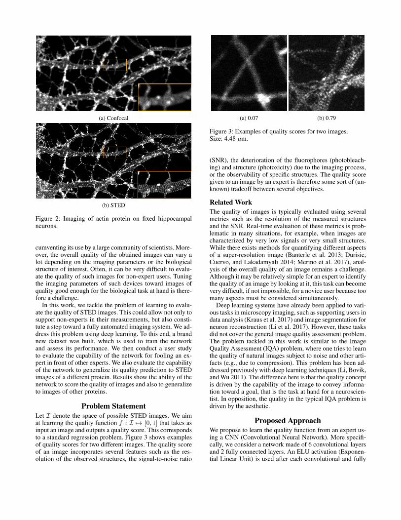
tion of fluorescent markers. Fluorophores are chemical com-pounds or proteins having the property of emitting light eachtime they are stimulated (excited) by a specific wavelength.These can be either coupled to antibodies (chemical com-pounds) that will recognize a protein of interest or fuseddirectly on the protein (fluorescent proteins) and thereforemake a structure visible on a fluorescence microscope. Us-ing the depletion beam, fluorophores can be switched from afluorescent on-state to a non-fluorescent dark state by meansof stimulated emission and, due to the donut shape of thedepletion beam, only the fluorophores in the middle of thedonut can still be detected. Saturation of the deactivation ef-fectively reduces the size of the diffraction-limited fluores-cent spots that is emitted by the fluorophores being imaged.Figure 1 shows fluorescence PSFs (Point Spread Functions)obtained by confocal and STED imaging of TetraSpeck mi-crospheres (100 nm), along with their merge. We observethat the STED image has a much higher resolution than theconfocal image. Moreover, we can see the donut shape onthe merged image. Figure 2 shows neurons images obtainedby confocal and STED microscopy. We observe that STEDmicroscopy allows us to observe a periodical lattice structureof the neuronal actin protein which is invisible with conven-tional confocal microscopy.

Super-resolution microscopes are highly specialized de-vices, significantly more complex to use than conventionaloptical microscopes. This reduces their accessibility, cir-

(a) Confocal

(b) STED

Figure 2: Imaging of actin protein on fixed hippocampalneurons.

cumventing its use by a large community of scientists. More-over, the overall quality of the obtained images can vary alot depending on the imaging parameters or the biologicalstructure of interest. Often, it can be very difficult to evalu-ate the quality of such images for non-expert users. Tuningthe imaging parameters of such devices toward images ofquality good enough for the biological task at hand is there-fore a challenge.

In this work, we tackle the problem of learning to evalu-ate the quality of STED images. This could allow not only tosupport non-experts in their measurements, but also consti-tute a step toward a fully automated imaging system. We ad-dress this problem using deep learning. To this end, a brandnew dataset was built, which is used to train the networkand assess its performance. We then conduct a user studyto evaluate the capability of the network for fooling an ex-pert in front of other experts. We also evaluate the capabilityof the network to generalize its quality prediction to STEDimages of a different protein. Results show the ability of thenetwork to score the quality of images and also to generalizeto images of other proteins.

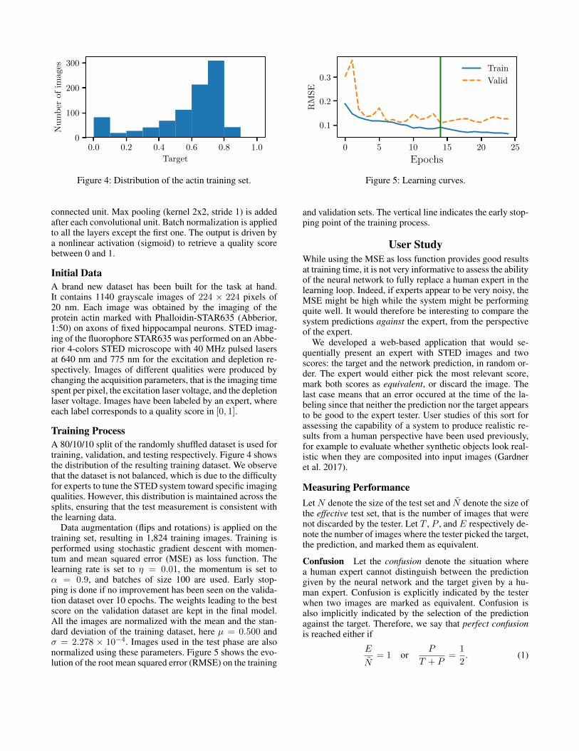
Problem StatementLet I denote the space of possible STED images. We aimat learning the quality function f : I 7→ [0, 1] that takes asinput an image and outputs a quality score. This correspondsto a standard regression problem. Figure 3 shows examplesof quality scores for two different images. The quality scoreof an image incorporates several features such as the res-olution of the observed structures, the signal-to-noise ratio

(a) 0.07 (b) 0.79

Figure 3: Examples of quality scores for two images.Size: 4.48 µm.

(SNR), the deterioration of the fluorophores (photobleach-ing) and structure (photoxicity) due to the imaging process,or the observability of specific structures. The quality scoregiven to an image by an expert is therefore some sort of (un-known) tradeoff between several objectives.

Related WorkThe quality of images is typically evaluated using severalmetrics such as the resolution of the measured structuresand the SNR. Real-time evaluation of these metrics is prob-lematic in many situations, for example, when images arecharacterized by very low signals or very small structures.While there exists methods for quantifying different aspectsof a super-resolution image (Banterle et al. 2013; Durisic,Cuervo, and Lakadamyali 2014; Merino et al. 2017), anal-ysis of the overall quality of an image remains a challenge.Although it may be relatively simple for an expert to identifythe quality of an image by looking at it, this task can becomevery difficult, if not impossible, for a novice user because toomany aspects must be considered simultaneously.

Deep learning systems have already been applied to vari-ous tasks in microscopy imaging, such as supporting users indata analysis (Kraus et al. 2017) and image segmentation forneuron reconstruction (Li et al. 2017). However, these tasksdid not cover the general image quality assessment problem.The problem tackled in this work is similar to the ImageQuality Assessment (IQA) problem, where one tries to learnthe quality of natural images subject to noise and other arti-facts (e.g., due to compression). This problem has been ad-dressed previously with deep learning techniques (Li, Bovik,and Wu 2011). The difference here is that the quality conceptis driven by the capability of the image to convey informa-tion toward a goal, that is the task at hand for a neuroscien-tist. In opposition, the quality in the typical IQA problem isdriven by the aesthetic.

Proposed ApproachWe propose to learn the quality function from an expert us-ing a CNN (Convolutional Neural Network). More specifi-cally, we consider a network made of 6 convolutional layersand 2 fully connected layers. An ELU activation (Exponen-tial Linear Unit) is used after each convolutional and fully

0.0 0.2 0.4 0.6 0.8 1.0

Target

0

100

200

300N

um

ber

of

imag

es

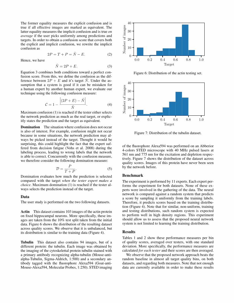
Figure 4: Distribution of the actin training set.

connected unit. Max pooling (kernel 2x2, stride 1) is addedafter each convolutional unit. Batch normalization is appliedto all the layers except the first one. The output is driven bya nonlinear activation (sigmoid) to retrieve a quality scorebetween 0 and 1.

Initial DataA brand new dataset has been built for the task at hand.It contains 1140 grayscale images of 224 × 224 pixels of20 nm. Each image was obtained by the imaging of theprotein actin marked with Phalloidin-STAR635 (Abberior,1:50) on axons of fixed hippocampal neurons. STED imag-ing of the fluorophore STAR635 was performed on an Abbe-rior 4-colors STED microscope with 40 MHz pulsed lasersat 640 nm and 775 nm for the excitation and depletion re-spectively. Images of different qualities were produced bychanging the acquisition parameters, that is the imaging timespent per pixel, the excitation laser voltage, and the depletionlaser voltage. Images have been labeled by an expert, whereeach label corresponds to a quality score in [0, 1].

Training ProcessA 80/10/10 split of the randomly shuffled dataset is used fortraining, validation, and testing respectively. Figure 4 showsthe distribution of the resulting training dataset. We observethat the dataset is not balanced, which is due to the difficultyfor experts to tune the STED system toward specific imagingqualities. However, this distribution is maintained across thesplits, ensuring that the test measurement is consistent withthe learning data.

Data augmentation (flips and rotations) is applied on thetraining set, resulting in 1,824 training images. Training isperformed using stochastic gradient descent with momen-tum and mean squared error (MSE) as loss function. Thelearning rate is set to η = 0.01, the momentum is set toα = 0.9, and batches of size 100 are used. Early stop-ping is done if no improvement has been seen on the valida-tion dataset over 10 epochs. The weights leading to the bestscore on the validation dataset are kept in the final model.All the images are normalized with the mean and the stan-dard deviation of the training dataset, here µ = 0.500 andσ = 2.278 × 10−4. Images used in the test phase are alsonormalized using these parameters. Figure 5 shows the evo-lution of the root mean squared error (RMSE) on the training

0 5 10 15 20 25

Epochs

0.1

0.2

0.3

RM

SE

Train

Valid

Figure 5: Learning curves.

and validation sets. The vertical line indicates the early stop-ping point of the training process.

User StudyWhile using the MSE as loss function provides good resultsat training time, it is not very informative to assess the abilityof the neural network to fully replace a human expert in thelearning loop. Indeed, if experts appear to be very noisy, theMSE might be high while the system might be performingquite well. It would therefore be interesting to compare thesystem predictions against the expert, from the perspectiveof the expert.

We developed a web-based application that would se-quentially present an expert with STED images and twoscores: the target and the network prediction, in random or-der. The expert would either pick the most relevant score,mark both scores as equivalent, or discard the image. Thelast case means that an error occured at the time of the la-beling since that neither the prediction nor the target appearsto be good to the expert tester. User studies of this sort forassessing the capability of a system to produce realistic re-sults from a human perspective have been used previously,for example to evaluate whether synthetic objects look real-istic when they are composited into input images (Gardneret al. 2017).

Measuring PerformanceLetN denote the size of the test set and N denote the size ofthe effective test set, that is the number of images that werenot discarded by the tester. Let T , P , and E respectively de-note the number of images where the tester picked the target,the prediction, and marked them as equivalent.

Confusion Let the confusion denote the situation wherea human expert cannot distinguish between the predictiongiven by the neural network and the target given by a hu-man expert. Confusion is explicitly indicated by the testerwhen two images are marked as equivalent. Confusion isalso implicitly indicated by the selection of the predictionagainst the target. Therefore, we say that perfect confusionis reached either if

E

N= 1 or

P

T + P=

1

2. (1)

The former equality measures the explicit confusion and istrue if all effective images are marked as equivalent. Thelatter equality measures the implicit confusion and is true onaverage if the user picks uniformly among predictions andtargets. In order to obtain a confusion score that covers boththe explicit and implicit confusion, we rewrite the implicitconfusion as

2P = T + P = N − E. (2)

Hence, we have

N = 2P + E. (3)

Equation 3 combines both conditions toward a perfect con-fusion score. From this, we define the confusion as the dif-ference between 2P + E and it’s target N . Under the as-sumption that a system is good if it can be mistaken fora human expert by another human expert, we evaluate ourtechnique using the following confusion measure:

C = 1−

∣∣∣(2P + E)− N∣∣∣

N. (4)

Maximum confusion (1) is reached if the tester either selectsthe network prediction as much as the real target, or explic-itly states the prediction and the target as equivalent.

Domination The situation where confusion does not occuris also of interest. For example, confusion might not occurbecause in some situations, the network prediction may al-ways be picked instead of the target. Thought it would besurprising, this could highlight the fact that the expert suf-fered from decision fatigue (Vohs et al. 2008) during thelabeling process, leading to wrong labels that the networkis able to correct. Concurrently with the confusion measure,we therefore consider the following domination measure:

D =P

T + P. (5)

Domination evaluates how much the prediction is selectedcompared with the target when the tester expert makes achoice. Maximum domination (1) is reached if the tester al-ways selects the prediction instead of the target.

DataThe user study is performed on the two following datasets.

Actin This dataset contains 103 images of the actin proteinon fixed hippocampal neurons. More specifically, these im-ages are taken from the 10% test split taken from the initialdata. Figure 6 shows the distribution of the resulting datasetacross quality scores. We observe that it is unbalanced, butits distribution is similar to the training data (Figure 4).

Tubulin This dataset also contains 94 images, but of adifferent protein: the tubulin. Each image was obtained bythe imaging of the cytoskelettal protein tubulin stained witha primary antibody recognizing alpha-tubulin (Mouse-anti-alpha-Tubulin, Sigma-Aldrich, 1:500) and a secondary an-tibody tagged with the fluorophore Alexa594 (Goat-anti-Mouse-Alexa594, Molecular Probes, 1:250). STED imaging

0.0 0.2 0.4 0.6 0.8 1.0

Target

0

10

20

30

40

Nu

mb

erof

images

Figure 6: Distribution of the actin testing set.

0.0 0.2 0.4 0.6 0.8 1.0

Target

0

10

20

30

40

Nu

mb

erof

images

Figure 7: Distribution of the tubulin dataset.

of the fluorophore Alexa594 was performed on an Abberior4-colors STED microscope with 40 MHz pulsed lasers at561 nm and 775 nm for the excitation and depletion respec-tively. Figure 7 shows the distribution of the dataset acrossquality scores. Images of this protein have never been seenby the network before.

BenchmarkThe experiment is performed by 11 experts. Each expert per-forms the experiment for both datasets. None of these ex-perts were involved in the gathering of the data. The neuralnetwork is compared against a random system that predictsa score by sampling it uniformly from the training labels.Therefore, it predicts scores based on the training distribu-tion (Figure 4). Note that for similar, non-uniform, trainingand testing distributions, such random system is expectedto perform well in high density regions. This experimentshould allow us to assess that the proposed neural networksystem is not limited to learning the training distribution.

ResultsTables 1 and 2 show these performance measures per binof quality scores, averaged over testers, with one standarddeviation. More specifically, the performance measures arecalculated for each tester and their scores are then averaged.

We observe that the proposed network approach beats therandom baseline in almost all target quality bins, on bothdatasets, and regarding both measures. Note that not enoughdata are currently available in order to make these results

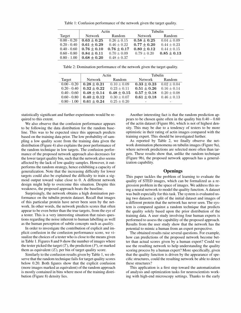
Table 1: Confusion performance of the network given the target quality.

Actin TubulinTarget Network Random Network Random0.00 - 0.20 0.63± 0.25 0.26± 0.15 0.58± 0.25 0.04± 0.090.20 - 0.40 0.61± 0.29 0.46± 0.22 0.77± 0.20 0.44± 0.230.40 - 0.60 0.76± 0.10 0.76± 0.17 0.80± 0.12 0.44± 0.150.60 - 0.80 0.84± 0.11 0.70± 0.09 0.79± 0.20 0.85± 0.130.80 - 1.00 0.68± 0.20 0.48± 0.37 - -

Table 2: Domination performance of the network given the target quality.

Actin TubulinTarget Network Random Network Random0.00 - 0.20 0.28± 0.21 0.10± 0.09 0.33± 0.23 0.02± 0.040.20 - 0.40 0.32± 0.22 0.23± 0.11 0.51± 0.26 0.16± 0.140.40 - 0.60 0.48± 0.14 0.48± 0.15 0.57± 0.18 0.20± 0.080.60 - 0.80 0.40± 0.12 0.30± 0.07 0.61± 0.18 0.46± 0.130.80 - 1.00 0.61± 0.24 0.25± 0.20 - -

statistically significant and further experiments would be re-quired to this extent.

We also observe that the confusion performance appearsto be following the data distribution for the random base-line. This was to be expected since this approach predictsbased on the training data prior. The low probability of sam-pling a low quality score from the training data given thedistribution (Figure 4) also explains the poor performance ofthe random technique in low targets. The confusion perfor-mance of the proposed network approach also decreases forthe lower target quality bin, such that the network also seemsaffected by the lack of low quality samples. However, it out-performs the random strategy, hence exhibiting a capacity ofgeneralization. Note that the increasing difficulty for lowertargets could also be explained the difficulty to train a sig-moid output toward value close to 0. A different networkdesign might help to overcome this situation. Despite thisweakness, the proposed approach beats the baseline.

Surprisingly, the network obtains a high domination per-formance on the tubulin protein dataset. Recall that imagesof this particular protein have never been seen by the net-work. In other words, the network predicts scores that oftenappear to be even better than the true targets, from the eye ofa tester. This is a very interesting situation that raises ques-tions regarding the noise inherent to human labelling as wellas the human perception of subtle concepts such as quality.

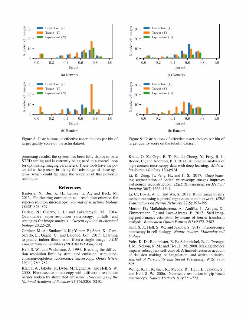
In order to investigate the contribution of explicit and im-plicit confusion in the confusion performance score, we vi-sualize the choices of a tester who is close to the means givenin Table 1. Figures 8 and 9 show the number of images wherethe tester picked the target (T ), the prediction (P ), or markedthem as equivalent (E), per bin of target quality score.

Similarly to the confusion results given by Table 1, we ob-serve that the random technique fails for target quality scoresbelow 0.20. Both figures show that the explicit confusion(more images marked as equivalent) of the random approachis mostly contained in bins where most of the training distri-bution (Figure 8) density lies.

Another interesting fact is that the random prediction ap-pears to be chosen quite often in the quality bin 0.40 – 0.60of the actin dataset (Figure 8b), which is not of highest den-sity. This may be due to a tendency of testers to be moreoptimistic in their rating of actin images compared with thetraining expert. This should be investigated further.

As reported by Table 2, we finally observe the net-work domination phenomena on tubulin images (Figure 9a),where network predictions are selected more often than tar-gets. These results show that, unlike the random technique(Figure 9b), the proposed network approach has a general-ization capability.

OpeningsThis paper tackles the problem of learning to evaluate thequality of STED images, which can be formalized as a re-gression problem in the space of images. We address this us-ing a neural network to model the quality function. A datasetwas built especially for this task. The system is evaluated us-ing two datasets: a split of the initial dataset and images ofa different protein that the network has never seen. The sys-tem is compared against a random technique that predictsthe quality solely based upon the prior distribution of thetraining data. A user study involving four human experts isperformed to assess the capability of the proposed approach.Results from the user study show that the network has thepotential to mimic a human from an expert perspective.

The obtained results raise several questions. For example,how can predictions of the proposed network become bet-ter than actual scores given by a human expert? Could weuse the resulting network to help understanding the qualityscoring process by a human expert? More specifically, giventhat the quality function is driven by the appearance of spe-cific structures, could the resulting network be able to detectthese structures?

This application is a first step toward the automatizationof analysis and optimization tasks for neuroscientists work-ing with high-end microscopy settings. Thanks to the early

0.0 0.2 0.4 0.6 0.8 1.0

Target

0

10

20

30

Nu

mb

erof

imag

es Prediction (P )

Target (T )

Equivalent (E)

(a) Network

0.0 0.2 0.4 0.6 0.8 1.0

Target

0

10

20

30

Nu

mb

erof

imag

es Prediction (P )

Target (T )

Equivalent (E)

(b) Random

Figure 8: Distributions of effective tester choices per bin oftarget quality score on the actin dataset.

promising results, the system has been fully deployed on aSTED setting and is currently being used in a control loopfor optimizing imaging parameters. These tools have the po-tential to help users in taking full advantage of these sys-tems, which could facilitate the adoption of this powerfultechnique.

ReferencesBanterle, N.; Bui, K. H.; Lemke, E. A.; and Beck, M.2013. Fourier ring correlation as a resolution criterion forsuper-resolution microscopy. Journal of structural biology183(3):363–367.Durisic, N.; Cuervo, L. L.; and Lakadamyali, M. 2014.Quantitative super-resolution microscopy: pitfalls andstrategies for image analysis. Current opinion in chemicalbiology 20:22–28.Gardner, M.-A.; Sunkavalli, K.; Yumer, E.; Shen, X.; Gam-baretto, E.; Gagne, C.; and Lalonde, J.-F. 2017. Learningto predict indoor illumination from a single image. ACMTransactions on Graphics (SIGGRAPH Asia) 9(4).Hell, S. W., and Wichmann, J. 1994. Breaking the diffrac-tion resolution limit by stimulated emission: stimulated-emission-depletion fluorescence microscopy. Optics letters19(11):780–782.Klar, T. A.; Jakobs, S.; Dyba, M.; Egner, A.; and Hell, S. W.2000. Fluorescence microscopy with diffraction resolutionbarrier broken by stimulated emission. Proceedings of theNational Academy of Sciences 97(15):8206–8210.

0.0 0.2 0.4 0.6 0.8 1.0

Target

0

10

20

30

Nu

mb

erof

imag

es Prediction (P )

Target (T )

Equivalent (E)

(a) Network

0.0 0.2 0.4 0.6 0.8 1.0

Target

0

10

20

30

Nu

mb

erof

imag

es Prediction (P )

Target (T )

Equivalent (E)

(b) Random

Figure 9: Distributions of effective tester choices per bin oftarget quality score on the tubulin dataset.

Kraus, O. Z.; Grys, B. T.; Ba, J.; Chong, Y.; Frey, B. J.;Boone, C.; and Andrews, B. J. 2017. Automated analysis ofhigh-content microscopy data with deep learning. Molecu-lar Systems Biology 13(4):924.Li, R.; Zeng, T.; Peng, H.; and Ji, S. 2017. Deep learn-ing segmentation of optical microscopy images improves3-d neuron reconstruction. IEEE Transactions on MedicalImaging 36(7):1533–1541.Li, C.; Bovik, A. C.; and Wu, X. 2011. Blind image qualityassessment using a general regression neural network. IEEETransactions on Neural Networks 22(5):793–799.Merino, D.; Mallabiabarrena, A.; Andilla, J.; Artigas, D.;Zimmermann, T.; and Loza-Alvarez, P. 2017. Sted imag-ing performance estimation by means of fourier transformanalysis. Biomedical Optics Express 8(5):2472–2482.Sahl, S. J.; Hell, S. W.; and Jakobs, S. 2017. Fluorescencenanoscopy in cell biology. Nature reviews. Molecular cellbiology.Vohs, K. D.; Baumeister, R. F.; Schmeichel, B. J.; Twenge,J. M.; Nelson, N. M.; and Tice, D. M. 2008. Making choicesimpairs subsequent self-control: A limited-resource accountof decision making, self-regulation, and active initiative.Journal of Personality and Social Psychology 94(5):883–898.Willig, K. I.; Kellner, R.; Medda, R.; Hein, B.; Jakobs, S.;and Hell, S. W. 2006. Nanoscale resolution in gfp-basedmicroscopy. Nature Methods 3(9):721–723.