learning to calibrate and rerank multi-label predictions · 2019-10-14 · makes accurate set...

Learning to Calibrate and Rerank Multi-labelPredictions

Cheng Li (�), Virgil Pavlu, Javed Aslam, Bingyu Wang, and Kechen Qin

Khoury College of Computer Sciences, Northeastern University, Boston, USA{chengli,vip,jaa,rainicy}@ccs.neu.edu, [email protected]

Abstract. A multi-label classifier assigns a set of labels to each dataobject. A natural requirement in many end-use applications is that theclassifier also provides a well-calibrated confidence (probability) to in-dicate the likelihood of the predicted set being correct; for example, anapplication may automate high-confidence predictions while manuallyverifying low-confidence predictions. The simplest multi-label classifier,called Binary Relevance (BR), applies one binary classifier to each labelindependently and takes the product of the individual label probabilitiesas the overall label-set probability (confidence). Despite its many knowndrawbacks, such as generating suboptimal predictions and poorly cali-brated confidence scores, BR is widely used in practice due to its speedand simplicity. We seek in this work to improve both BR’s confidenceestimation and prediction through a post calibration and reranking pro-cedure. We take the BR predicted set of labels and its product scoreas features, extract more features from the prediction itself to capturelabel constraints, and apply Gradient Boosted Trees (GB) as a calibratorto map these features into a calibrated confidence score. GB not onlyproduces well-calibrated scores (aligned with accuracy and sharp), butalso models label interactions, correcting a critical flaw in BR. We fur-ther show that reranking label sets by the new calibrated confidencemakes accurate set predictions on par with state-of-the-art multi-labelclassifiers—yet calibrated, simpler, and faster.

Keywords: Multi-label classification · Confidence score calibration ·Reranking

1 Introduction

Multi-label classification is an important machine learning task wherein onepredicts a subset of labels to associate with a given object. For example, anarticle can belong to multiple categories; an image can be associated with severaltags; in medical billing, a patient report is annotated with multiple diagnosiscodes. Formally, in a multi-label classification problem, we are given a set of labelcandidates Y = {1, 2, ..., L}. Every data point x ∈ RD matches a subset of labelsy ⊆ Y , which is typically written in the form of a binary vector y ∈ {0, 1}L, witheach bit y` indicating the presence or absence of the corresponding label. The

2 C. Li et al.

goal of learning is to build a classifier h : RD → {0, 1}L which maps an instanceto a subset of labels. The predicted label subset can be of arbitrary size.

The simplest approach to multi-label classification is to apply one binaryclassifier (e.g., binary logistic regression or support vector machine) to predicteach label separately. This approach is called binary relevance (BR) [35] and iswidely used due to its simplicity and speed. BR’s training time grows linearlywith the number of labels, which is considerably lower than many methods thatseek to model label dependencies, and this makes BR run reasonably fast oncommonly used datasets. (Admittedly, BR may still fail to scale to datasets withextremely large number of labels, in which case specially designed multi-labelclassifiers with sub-linear time complexity should be employed instead. But inthis paper, we shall not consider such extreme multi-label classification problem.)

BR has two well-known drawbacks. First, BR neglects label dependenciesand this often leads to prediction errors: some BR predictions are incomplete,such as tagging cat but not animal for an image, and some are conflicting,such as predicting both the code Pain in left knee and the code Pain in

unspecified knee for a medical note. Second, the confidence score or probability(we shall use “confidence score” and “probability” interchangeably) BR associatesto its overall set prediction y is often misleading, or uncalibrated. BR computesthe overall set prediction confidence score as the product of the individual labelconfidence scores, i.e., p(y|x) =

∏Ll=1 p(yl|x). This overall confidence score often

does not reflect reality: among all the set predictions on which BR claims tohave roughly 80% confidence, maybe only 60% of them are actually correct (apredicted set is considered “correct” if it matches the ground truth set exactly).Having such uncalibrated prediction confidence makes it hard to integrate BRdirectly into a decision making pipeline where not only the predictions but alsothe confidence scores are used in downstream tasks.

In this work, we seek to address these two issues associated with BR. Wefirst improve the BR set prediction confidence scores though a feature-based postcalibration procedure to make confidence scores indicative of the true set accuracy(described in Section 2). The features considered in calibration capture labeldependencies that have otherwise been missing in standard BR. Next we improveBR’s set prediction accuracy by reranking BR’s prediction candidates using thenew calibrated confidence scores (described in Section 3). There exist multi-labelmethods that avoid the label independence assumption from the beginning andperform joint probability estimations [30, 7, 22, 13, 9, 23]; such methods oftenrequire more complex training and inference procedures. In this paper we showthat BR base model together with our proposed post calibration/rerankingmakes accurate set predictions on par with (or better than) these state-of-the-artmulti-label methods —yet calibrated, simpler, and faster.

2 Calibrate BR Multi-label Predictions

We first address BR’s confidence mis-calibration issue. There are two types ofconfidence scores in BR: the confidence of an individual label prediction p(yl|x),

Learning to Calibrate and Rerank Multi-label Predictions 3

and the confidence of the entire predicted set p(y|x). In this work we take forgranted that the individual label scores have already been calibrated, whichcan be easily done with established univariate calibration procedures such asisotonic regression [31] or Platt scaling [39, 28]. We are concerned here with theset confidence calibration; note that calibrating all individual label confidencescores does not automatically calibrate set prediction confidence scores.

2.1 Metrics for Calibration: Alignment Error, Sharpness and MSE

To describe our calibration method, we need the following formal definitions:• c(y) ∈ [0, 1] is the confidence score associated with the set prediction y;• v(y) ∈ {0, 1} is the 0/1 correctness of set prediction y;• e(c) = p[v(y) = 1|c(y) = c] is the average set accuracy among all predictionswhose confidence is c. In practice, this is estimated by bucketing predictionsbased on confidence scores and computing the average accuracy for each bucket.

We use the following standard metrics for calibration [21]:• Alignment error, defined as Ey[e(c(y)) − c(y)]2, measures, on average overall predictions, the discrepancy between the claimed confidence and the actualaccuracy. The smaller the better.• Sharpness, defined as Vary[e(c(y))], measures how widely spread the confidencescores are. The bigger the better.• The mean squared error (MSE, also called Brier Score) defined as Ey[(v(y)−c(y))2], measures the difference between the confidence and the actual 0/1 cor-rectness. It can be decomposed into alignment error, sharpness and an irreducibleconstant “uncertainty” due to only classification (not calibration) error [21]:

Ey[(v(y)− c(y))2]︸︷︷︸MSE

= Vary[v(y)]︸︷︷︸uncertainty

−Vary[e(c(y))]︸︷︷︸sharpness

+Ey[(e(c(y))− c(y))2]︸︷︷︸alignment error

(1)

Alignment error and sharpness capture two orthogonal aspects of confidencecalibration. A small alignment error implies that the confidence score is wellaligned with the actual accuracy. However, small alignment error, alone, is notmeaningful: the calibration can trivially achieve zero alignment error while beingcompletely uninformative by assigning to all predictions the same confidencescore, which is the average accuracy among all predictions on the dataset. Auseful calibrator should also separate good predictions from bad ones as much aspossible by assigning very different confidence scores to them. In other words, agood calibrator should simultaneously minimize alignment error and maximizesharpness. This can be achieved by minimizing MSE, thus MSE makes a naturalobjective for calibrator training. Minimizing MSE leads to a standard regressiontask: one can simply train a regressor c that maps each prediction y to its binarycorrectness v(y). Note that training a calibrator by optimizing MSE does notrequire estimation of e(c(y)), but evaluating its sharpness and alignment errordoes. Estimating e(c(y)) by bucketing predictions has some subtle issues, as weshall explain later when we present evaluation results in Section 2.4.

4 C. Li et al.

2.2 Features for Calibration

Besides the training objective, we also need to decide the parametric form of thecalibrator and the features to be used. In order to explain the choices we make,we shall use the calibration on WISE dataset1 as a running example.

0.0 0.2 0.4 0.6 0.8 1.0uncalibrated confidence

0.0

0.2

0.4

0.6

0.8

1.0

accura

cy

mse=0.241uncertainty=0.246align err=0.017sharpness=0.021

all predictions

(a)


0.0

0.2

0.4

0.6

0.8

1.0

accura

cy

all predictions

(b)


0.0

0.2

0.4

0.6

0.8

1.0

accura

cy

card=0

card=1

card=2

(c)


0.0

0.2

0.4

0.6

0.8

1.0

accura

cy

popular

rare

new

(d)

0.0 0.2 0.4 0.6 0.8 1.0calibrated confidence

0.0

0.2

0.4

0.6

0.8

1.0

accura

cy

mse=0.246uncertainty=0.246align err=0sharpness=0

all predictions

(e)


0.0

0.2

0.4

0.6

0.8

1.0

accura

cy

mse=0.223uncertainty=0.246align err=3x10^-4sharpness=0.022

all predictions

(f)


0.0

0.2

0.4

0.6

0.8

1.0accura

cy


card=0

card=1

card=2

(g)


0.0

0.2

0.4

0.6

0.8

1.0

accura

cy


popular

rare

new

(h)

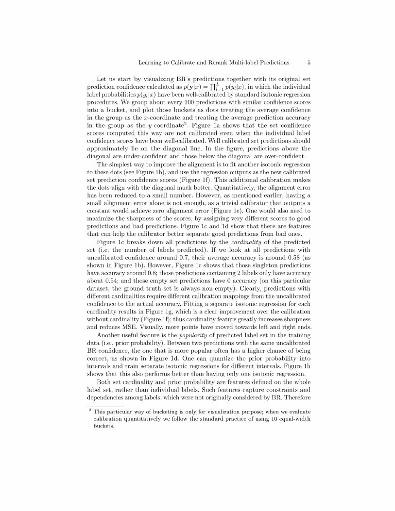
Fig. 1: Multi-label set prediction confidence vs. set prediction accuracy on theWISE dataset. In all sub-figures, each dot represents a group of 100 set predictionswith similar confidence scores. The average confidence score in the group is usedas x-coordinate, and the average prediction accuracy is used as y-coordinate. (a)BR predictions with the original BR confidence scores. (e) Trivial calibrationthat gives all predictions the same confidence score which is the overall setaccuracy on the dataset. (b) Isotonic regression (the solid line) trained on allpredictions. (f) Predictions with isotonic regression calibrated confidence. (c)Break down all predictions by the set cardinality and train a separate isotonicregression (the solid line) for each cardinality. (g) Predictions with confidencecalibrated by cardinality-based isotonic regressions. (d) Group all predictionsinto 3 categories by the popularity of predicted label combination in the trainingdata ground truth (popular=the predicted label combination appears at least100 times; rare=the predicted label combination appears less than 100 times;new=the predicted label combination does not appear at all in training data),and train a separate isotonic regression (the solid line) for each category. (h)Predictions with confidence calibrated by popularity-based isotonic regressions.To simplify the presentation, all calibrators are trained and evaluated on thesame data.

1 https://www.kaggle.com/c/wise-2014/data


Let us start by visualizing BR’s predictions together with its original setprediction confidence calculated as p(y|x) =

∏Ll=1 p(yl|x), in which the individual

label probabilities p(yl|x) have been well-calibrated by standard isotonic regressionprocedures. We group about every 100 predictions with similar confidence scoresinto a bucket, and plot those buckets as dots treating the average confidencein the group as the x-coordinate and treating the average prediction accuracyin the group as the y-coordinate2. Figure 1a shows that the set confidencescores computed this way are not calibrated even when the individual labelconfidence scores have been well-calibrated. Well calibrated set predictions shouldapproximately lie on the diagonal line. In the figure, predictions above thediagonal are under-confident and those below the diagonal are over-confident.

The simplest way to improve the alignment is to fit another isotonic regressionto these dots (see Figure 1b), and use the regression outputs as the new calibratedset prediction confidence scores (Figure 1f). This additional calibration makesthe dots align with the diagonal much better. Quantitatively, the alignment errorhas been reduced to a small number. However, as mentioned earlier, having asmall alignment error alone is not enough, as a trivial calibrator that outputs aconstant would achieve zero alignment error (Figure 1e). One would also need tomaximize the sharpness of the scores, by assigning very different scores to goodpredictions and bad predictions. Figure 1c and 1d show that there are featuresthat can help the calibrator better separate good predictions from bad ones.

Figure 1c breaks down all predictions by the cardinality of the predictedset (i.e. the number of labels predicted). If we look at all predictions withuncalibrated confidence around 0.7, their average accuracy is around 0.58 (asshown in Figure 1b). However, Figure 1c shows that those singleton predictionshave accuracy around 0.8; those predictions containing 2 labels only have accuracyabout 0.54; and those empty set predictions have 0 accuracy (on this particulardataset, the ground truth set is always non-empty). Clearly, predictions withdifferent cardinalities require different calibration mappings from the uncalibratedconfidence to the actual accuracy. Fitting a separate isotonic regression for eachcardinality results in Figure 1g, which is a clear improvement over the calibrationwithout cardinality (Figure 1f); thus cardinality feature greatly increases sharpnessand reduces MSE. Visually, more points have moved towards left and right ends.

Another useful feature is the popularity of predicted label set in the trainingdata (i.e., prior probability). Between two predictions with the same uncalibratedBR confidence, the one that is more popular often has a higher chance of beingcorrect, as shown in Figure 1d. One can quantize the prior probability intointervals and train separate isotonic regressions for different intervals. Figure 1hshows that this also performs better than having only one isotonic regression.

Both set cardinality and prior probability are features defined on the wholelabel set, rather than individual labels. Such features capture constraints anddependencies among labels, which were not originally considered by BR. Therefore

2 This particular way of bucketing is only for visualization purpose; when we evaluatecalibration quantitatively we follow the standard practice of using 10 equal-widthbuckets.

6 C. Li et al.

these features supplement BR’s own prediction score and allow the calibrator tomake better overall judgments on the predicted set. There can be other featuresthat help the calibrator better judge set predictions. In order to incorporatearbitrary number of features and avoid manual partitioning of the data andtraining separate calibrators (which quickly becomes infeasible as the numberof features grows), a general multi-variate regressor should be employed. Themulti-variate extension of isotonic regression exists [32], but it is not well suitedto our problem because some features such as cardinality do not have a monotonicrelationship with the calibrated confidence (see Figure 1c). [21] proposes KNNand regression trees as calibrators for general structured prediction problem.

2.3 Calibrator Model Training

In this work, we choose Gradient Boosted Trees (GB) [11] as the calibratormodel. Similar to regression trees, GB as a multi-variate regressor automaticallypartitions the prediction’s feature space into regions and outputs (approximately)the average prediction accuracy in each region as the calibrated confidence score.GB often produces smoother output than trees and generalizes better. GB isalso very powerful in modeling complex feature interactions automatically bybuilding many trees on top of the features. To leverage its power we also use thebinary representation of the set prediction y itself as features for GB. This wayGB can discover additional rules concerning certain label interactions that arenot described by the manually designed features (for example, “if two conflictinglabels A and B are both predicted, the prediction is never correct, thereforelower the confidence score”). It is also possible to use instance features x duringcalibration, but we do not find it helpful because BR was already built on x.

There are two commonly used GB variants [11]. The first variant, GB-MSE,uses the tree ensemble score as the output, and MSE as the training objective.The second variant, GB-KL, adds a sigmoid transformation to the ensemble scoreand uses KL-divergence as the training objective. GB-MSE has the advantageof directly minimizing MSE, which matches the evaluation metric used forcalibration (see section 2.1). But it has the disadvantage that its output is notbounded between 0 and 1 and one has to clip its output in order to treat that asa confidence score.

GB-KL has the advantage of providing bounded output, but its trainingobjective does not directly match the evaluation metric used for calibration;note, however, that minimizing KL-divergence also encourages the model outputto match the average prediction accuracy, hence achieves the calibration effect.It may appear that one could get the best of both worlds by having sigmoidtransformation and MSE training objective at the same time. Unfortunately,adding sigmoid makes MSE a non-convex function of the ensemble scores, thushard to optimize. In this paper, we choose GB-MSE as our GB calibrator andshall simply call it GB from now on. In supplementary material, we show thatGB-KL has very similar performance.

Each BR set prediction is transformed to a feature vector (containing orig-inal BR confidence score, set cardinality, set prior probability, and set binary


representation) and the binary correctness of the prediction is used as the re-gression target. Since the goal of GB calibrator is to objectively evaluate BR’sprediction accuracy, it is critical that the calibration data to be disjoint from theBR classifier training data. Otherwise, when BR over-fits its training data, thecalibrator will see over-optimistic results on the same data and learn to generateover-confident scores. Similarly, it is also necessary to further separate the labelcalibration data and the set calibration data, since the product of the calibratedlabel probabilities is used as input to the set calibrator training.

Imposing Partial Monotonicity Imposing monotonicity is a standard prac-tice in univariate calibration methods such as isotonic regression [31] and Plattscaling [39, 28] as it avoids over-fitting and leads to better interpretability. Im-posing (partial) monotonicity for a multi-variate calibrator is more challenging.Certain features considered in calibration are expected to be monotonically re-lated to the confidence. For example, the confidence should always increase withthe popularity (prior probability) of the predicted set, if all other features of theprediction are unchanged. The same is true for BR score. The rest of the features,including the cardinality of the set and the binary representation of the set, donot have monotonic relations with confidence. Therefore the calibration functionis partially monotonic. We have done additional experiments on imposing partialmonotonicity for the GB calibrator but did not observe significant improvement(details and experiment results are in supplementary material).

2.4 Calibration Results

Table 1: Datasets characteristics; label sets =number of label combinations in training set;cardinality = average number of labels per in-stance; inst/label = the average number of traininginstances per label. Datasets are obtained fromhttp://mulan.sourceforge.net/datasets-

mlc.html, http://cocodataset.org andhttps://www.kaggle.com/c/wise-2014/data

Dataset BIBTEX OHSUMED RCV1 TMC WISE MSCOCOdomain bkmark medical news reports articles imagelabels 159 23 103 22 203 80

label sets 2,173 968 622 1,104 2,782 19,597features 1,836 12,639 47,236 49,060 301,561 4,096instances 7,395 13,929 6,000 28,596 48,643 123,287

cardinality 2.40 1.68 3.21 2.16 1.45 2.90inst/label 89 811 150 2,244 278 3,572

We test the proposed GBcalibrator for BR set pre-dictions on 6 commonlyused multi-label datasets(see Table 1 for details).Each dataset is randomlysplit into training, cali-bration, validation andtest subsets. BR modelwith logistic regressionbase learners is trainedon training data; isotonicregression label calibra-tors and GB set calibra-tors are trained on (dif-ferent parts of) calibra-tion data. All hyper pa-rameters in BR and cali-brators are tuned on val-idation data. Calibration

8 C. Li et al.

results are reported ontest data.

For comparison, we consider the following calibrators:

• uncalib: use the uncalibrated BR probability as it is;• isotonic: calibrate the BR probability with isotonic regression;• card isotonic: for each label set cardinality, train one isotonic regression;• tree: use the features considered by GB, train a single regression tree.

To make a fair comparison, for all methods, individual label probabilities havealready been calibrated by isotonic regressions. We focus on their abilities tocalibrate set predictions. BR prediction is made by thresholding each label’sprobability (calibrated by isotonic regression) at 0.5. This corresponds to the setwith the highest BR score.

Table 2: BR prediction calibration performance in terms of MSE (the smallerthe better) and sharpness (the bigger the better). Bolded numbers are the best.

Dataset uncentaintyuncalib isotonic card isotonic tree GB

MSE sharp MSE sharp MSE sharp MSE sharp MSE sharp

BIBTEX 0.133 0.193 0.007 0.140 0.002 0.109 0.038 0.086 0.065 0.068 0.072OHSUMED 0.232 0.226 0.015 0.221 0.013 0.182 0.051 0.211 0.039 0.189 0.047RCV1 0.247 0.175 0.077 0.175 0.075 0.159 0.093 0.134 0.129 0.123 0.126TMC 0.212 0.192 0.019 0.192 0.020 0.192 0.022 0.194 0.029 0.180 0.032WISE 0.249 0.252 0.017 0.234 0.017 0.151 0.098 0.166 0.093 0.147 0.102MSCOCO 0.227 0.158 0.075 0.151 0.075 0.150 0.076 0.163 0.070 0.143 0.083

The evaluation metrics we use are MSE, sharpness and alignment error, asdescribed in Section 2.1. Following the standard practice, we use 10 equal-widthbuckets to estimate sharpness and alignment error. One issue with evaluation bybucketing is that using different number of buckets leads to different estimations ofalignment error and sharpness (but not MSE and uncertainty, whose computationsdo not depends on bucketing). In fact, increasing the number of buckets willincrease both the estimated alignment error and sharpness by the same amount,due to Eq 1. Using 10 buckets often produces negligible alignment error (relativeto MSE), and the comparison effectively focuses on sharpness. This amounts tomaximizing sharpness subject to a very small alignment error [14], which is oftena reasonable goal in practice. All calibrators are able to achieve small alignmenterror (on the order of 10−3 and contributing to less than 10% of the MSE), sowe do not report that. The results are summarized in Table 2. All calibratorsimprove upon the BR uncalibrated probabilities. Our GB calibrator achieves theoverall best MSE and sharpness calibration performance, due to use of additionalfeatures extracted from set predictions.


3 Rerank Multi-label Predictions

Now we aim to improve BR’s prediction accuracy, by fixing some of the predictionmistakes BR made due to ignoring label dependencies. Our solution is based onthe calibrator we just developed. Traditionally, the only role of a calibrator is tomap an uncalibrated confidence score to a calibrated confidence score. In thatsense the calibrator usually does not affect the classification, only the confidence.In fact, popular univariate calibrators such as isotonic regression and Platt scalingimplement monotonic functions, thus preserve the ranking/argmax of predictions.For our multi-variate GB calibrator, however, this is not the case. Even if weconstrain the calibrated confidence to be monotonically increasing with the BRprediction scores, there are still other features that may affect the ranking; inparticular the argmax predictions before and after calibration might be differenty sets. If indeed different, the prediction based on calibrated confidence takesinto account label dependencies and other constraints (which BR does not), andis more likely to be the correct set (even when the calibrated confidence is notvery high in absolute terms). Table 3 shows two such examples on the MSCOCOimage dataset. Therefore we can also use GB as a multi-label wrapper on top ofBR to rerank its predictions. We name this method as BR-rerank .

To do so, we use a two stage prediction pipeline. For each test instance x,we first list the top K label set candidates y by highest BR uncalibrated scores.This can be done efficiently using a dynamic programming procedure whichtakes advantage of the label independence assumption made in BR, describedin [23], and included in the supplementary material of this paper for the sakeof completeness. Although the label independence assumption does not hold inpractice, we find empirically that when K is reasonably large (e.g., K = 50), thecorrect y is often included in the top-K list. The chance that the correct answeris included in the top-K list is commonly called “oracle accuracy”, and it is anupper bound of the final prediction accuracy. Empirically, we observe the oracleaccuracy to be much higher than the final prediction accuracy, indicating thatthe candidate generation stage is not a bottleneck of final performance.

Prediction stage two: send the top set candidates with their scores and addi-tional features to the GB calibrator, and select the one with the highest calibratedconfidence as the final prediction. The calibrator has to be trained on more thantop-1 BR candidates (on a separate calibration dataset) to evaluate correctlyprediction candidates, so we train the GB calibrator on top-K candidates.

3.1 Conceptual Comparison with Related Multi-label Classifiers

Although the proposed BR-rerank classifier has a very simple design, it hassome advantages over many existing multi-label classifiers. Here we make someconceptual comparisons between BR-rerank and related multi-label classifiers.

BR-rerank can be seen as a stacking method in which a stage-1 model providesinitial estimations and a stage-2 model uses these estimations as input and makesthe final decision. There are other stacking methods proposed in the literature,and the two most well-known ones are called 2BR [15, 34] and DBR [25]. The

10 C. Li et al.

Table 3: Predictions made by standard BR vs predictions made by rerankingBR predictions based on calibrated confidence. For each image, the top rowshows the top-5 set prediction candidates generated by BR. Numbers after“BR” are uncalibrated confidence. Numbers after “BR-rerank” are calibratedconfidence. Top image: BR predicts {person,baseball bat} with confidence0.58. BR-rerank predicts the correct set {person, baseball bat, baseball

glove} with confidence 0.17. Bottom image: BR predicts {person, remote,

toothbrush} with confidence 0.70. BR-rerank predicts the correct set {person,remote} with confidence 0.18.

person, person, person, person, person,

baseball bat baseball bat, handbag, sports ball, handbag,

y candidates baseball glove baseball bat baseball bat baseball bat,

baseball glove

BR 0.58* 0.35 0.02 0.02 0.01

BR-rerank 0.16 0.17* 0.04 0.08 0.03

person, person, person, person person,

remote, remote toothbrush tennis racket,

y candidates toothbrush remote,

toothbrush

BR 0.70* 0.24 0.03 0.01 0.01

BR-rerank 0.16 0.18* 0.05 0.02 0.01

stage-1 models in 2BR and DBR are also BR models just as in BR-rerank. Thestage-2 models in 2BR and DBR work differently. In 2BR, the stage-2 modelpredicts each label ` with a separate binary classifier which takes as input theoriginal instance feature vector x as well as all label probabilities predictedby the stage-1 model. In DBR, the stage-2 model predicts each label ` with aseparate binary classifier which takes as input the original instance feature vector


x as well as the binary absence/presence information of all other labels. Theabsence/presence of label ` itself is not part of the input to avoid learning a trivialmapping. During training, the absence/presence information is obtained from theground truth; during prediction, it is obtained from the stage-1 model’s prediction.Clearly for DBR there is some inconsistency on how stage-2 inputs are obtained.BR-rerank and 2BR do not suffer from such inconsistency. All three stackingmethods BR-rerank, 2BR, and DBR try to incorporate label dependencies intofinal classification. However, both 2BR and DBR have a critical flaw: when theirstage-2 models make the final decision for a particular label, they do not reallytake into account the final decisions made for other labels by the stage-2 model;they instead only consider the initial estimations on other labels made by thestage-1 model, which can be quite different. As a result, the final set predictionsmade by 2BR and DBR may not respect the label dependencies/constraintsthese models have learned. By contrast, the stage-2 model in BR-rerank directlyevaluates the final set prediction (based on its binary representation and otherextracted features) to make sure that the final set prediction satisfies the desiredlabel dependencies/constraints. For example, in the RCV1 dataset, each instancehas at least one label. But DBR predicted the empty set on 6% of the testinstances. By contrast, BR-rerank never predicted empty set on this dataset.

Many multi-label methods avoid the label independence assumption made inBR and model the joint distribution p(y|x) in more principled ways. Examplesinclude Conditional Random Fields (CRF) [13], Conditional Bernoulli Mixtures(CBM) [23], and Probabilistic Classifier Chains (PCC) [30, 7, 22, 24]. Despite thejoint estimation formulation, CRF, CBM, and PCC in practice often produceover-confident set prediction confidence scores, due to overfitting. Their predictionconfidence must also be post-calibrated.

The pair-wise CRF model [13] captures pairwise label interactions by estimat-ing 4 parameters for each label pair. However, because the model needs to assigndedicated parameters to different label combinations, modeling higher order labeldependencies becomes infeasible. The BR-rerank approach we propose relies onboosted trees to automatically build high order interactions as tree learns theirsplits on the binary representation of the label set – there is no need to allocateparameters in advance. There is another CRF model designed specifically tocapture exclusive or hierarchical label relations [9]; this works only when thelabel dependency graph is strict and a priori known.

CBM is a latent variable model and represents the joint as a mixture of binaryrelevance models. However, it is hard to directly control the kinds of dependenciesCBM learns, or to enforce constraints in the prediction. For example, CBM oftenpredicts the empty set even on dataset where empty prediction is not allowed.There is no easy way to enforce the cardinality constraint in CBM.

PCC decomposes the joint p(y|x) into a product of conditional probabilitiesp(y1|x)p(y2|x, y1) · · · p(yL|x, y1, .., yL−1), and reduces a multi-label problem toL binary problems, each of which learns a new label given all previous labels.However, different label chaining orders can lead to different results, and to find

12 C. Li et al.

the best order is often a challenge. In BR-rerank, all labels are treated as featuresin the GB calibrator training and they are completely symmetric.

The Structured Prediction Energy Network (SPEN) [1] uses deep neuralnetworks to efficiently encode arbitrary relations between labels, which to largedegree avoids parameterization issue associated with pair-wise CRF, but it cannotgenerate a confidence score for its MAP prediction as computing the normalizationconstant is intractable. The Predict-and-Constraint method (PC) [2] specificallyhandles cardinality constraint (but not other label constraints or relations) duringlearning and prediction. Deep value network (DVN) [18] trains a neural networkto evaluate prediction candidates and then uses back-propagation to find theprediction that leads to the maximum score. The idea is similar to our BR-rerankidea. The difference is: DVN could only use the binary encoding of the label set,but not any higher level features extracted from the label set, such as cardinalityand prior set probability. That is because its gradient based inference makes itvery difficult to directly incorporate such features. There are methods that seekto rank labels [3, 12]. Our method differs from theirs in that we rank label setsas opposed to individual labels, and we take into account label dependencies inthe label set.

3.2 Classification Results

We test the proposed BR-rerank classifier on 6 popular multi-label datasets (seeTable 1 for details). All datasets used in experiments contain at least a fewthousands instances. We do not take datasets with only a few hundred instancesas their testing performance tends to be quite unstable. We also do not considerdatasets with extremely large number of labels as our method is not designed forextreme classification (our method aims to maximize set accuracy but on extremedata it is very unlikely to predict the entire label set correctly due to large label setcardinality and annotation noise). We compare BR-rerank with many other well-known multi-label methods: Binary Relevance (BR) [35], 2BR [15, 34], DBR [25],pair-wise Conditional Random Field (CRF) [13], Conditional Bernoulli Mixture(CBM) [23], Probabilistic Classifier Chain (PCC) [30], Structured Prediction En-ergy Network (SPEN) [1], PD-Sparse (PDS) [38], Predict-and-Constrain (PC) [2],Deep value network (DVN) [18], Multi-label K-nearest neighbors (ML-KNN) [41],and Random k-label-sets (RAKEL) [36].

For evaluation, we report set accuracy and instance F1, defined as:

set accuracy =1

N

N∑n=1

I(y(n) = y(n)); instance F1 =1

N

N∑n=1

2∑L

l=1 y(n)l y

(n)l∑L

l=1 y(n)l +

∑Ll=1 y

(n)l

,

where y(n) and y(n) are the ground truth and predicted label set for the n-th in-stance, and I(y(n) = y(n)) returns 1 when the prediction is perfect and 0 otherwise.

Table 5: Training time of different methods,measured in seconds. All algorithms run multi-threaded on a server with 56 cores.

Dataset BIBT OHSUM RCV1 TMC WISE MSCOBR 4 3 7 8 80 1380

BR-rerank 9 6 10 11 88 1393CBM 64 210 70 224 1320 8520CRF 353 268 1223 771 16363 14760

To make a fair comparison,we use logistic regressions as theunderlying learners for BR as


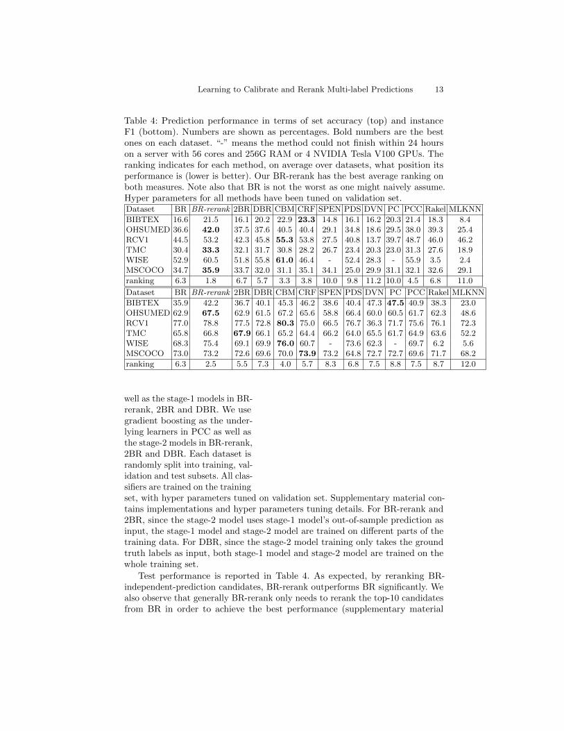
Table 4: Prediction performance in terms of set accuracy (top) and instanceF1 (bottom). Numbers are shown as percentages. Bold numbers are the bestones on each dataset. “-” means the method could not finish within 24 hourson a server with 56 cores and 256G RAM or 4 NVIDIA Tesla V100 GPUs. Theranking indicates for each method, on average over datasets, what position itsperformance is (lower is better). Our BR-rerank has the best average ranking onboth measures. Note also that BR is not the worst as one might naively assume.Hyper parameters for all methods have been tuned on validation set.Dataset BR BR-rerank 2BR DBR CBM CRF SPEN PDS DVN PC PCC Rakel MLKNN

BIBTEX 16.6 21.5 16.1 20.2 22.9 23.3 14.8 16.1 16.2 20.3 21.4 18.3 8.4OHSUMED 36.6 42.0 37.5 37.6 40.5 40.4 29.1 34.8 18.6 29.5 38.0 39.3 25.4RCV1 44.5 53.2 42.3 45.8 55.3 53.8 27.5 40.8 13.7 39.7 48.7 46.0 46.2TMC 30.4 33.3 32.1 31.7 30.8 28.2 26.7 23.4 20.3 23.0 31.3 27.6 18.9WISE 52.9 60.5 51.8 55.8 61.0 46.4 - 52.4 28.3 - 55.9 3.5 2.4MSCOCO 34.7 35.9 33.7 32.0 31.1 35.1 34.1 25.0 29.9 31.1 32.1 32.6 29.1

ranking 6.3 1.8 6.7 5.7 3.3 3.8 10.0 9.8 11.2 10.0 4.5 6.8 11.0

Dataset BR BR-rerank 2BR DBR CBM CRF SPEN PDS DVN PC PCC Rakel MLKNN

BIBTEX 35.9 42.2 36.7 40.1 45.3 46.2 38.6 40.4 47.3 47.5 40.9 38.3 23.0OHSUMED 62.9 67.5 62.9 61.5 67.2 65.6 58.8 66.4 60.0 60.5 61.7 62.3 48.6RCV1 77.0 78.8 77.5 72.8 80.3 75.0 66.5 76.7 36.3 71.7 75.6 76.1 72.3TMC 65.8 66.8 67.9 66.1 65.2 64.4 66.2 64.0 65.5 61.7 64.9 63.6 52.2WISE 68.3 75.4 69.1 69.9 76.0 60.7 - 73.6 62.3 - 69.7 6.2 5.6MSCOCO 73.0 73.2 72.6 69.6 70.0 73.9 73.2 64.8 72.7 72.7 69.6 71.7 68.2

ranking 6.3 2.5 5.5 7.3 4.0 5.7 8.3 6.8 7.5 8.8 7.5 8.7 12.0

well as the stage-1 models in BR-rerank, 2BR and DBR. We usegradient boosting as the under-lying learners in PCC as well asthe stage-2 models in BR-rerank,2BR and DBR. Each dataset israndomly split into training, val-idation and test subsets. All clas-sifiers are trained on the trainingset, with hyper parameters tuned on validation set. Supplementary material con-tains implementations and hyper parameters tuning details. For BR-rerank and2BR, since the stage-2 model uses stage-1 model’s out-of-sample prediction asinput, the stage-1 model and stage-2 model are trained on different parts of thetraining data. For DBR, since the stage-2 model training only takes the groundtruth labels as input, both stage-1 model and stage-2 model are trained on thewhole training set.

Test performance is reported in Table 4. As expected, by reranking BR-independent-prediction candidates, BR-rerank outperforms BR significantly. Wealso observe that generally BR-rerank only needs to rerank the top-10 candidatesfrom BR in order to achieve the best performance (supplementary material

14 C. Li et al.

shows how its performance changes as K increases). On each dataset, we rankall algorithms by performance, and report each algorithm’s average rankingacross all datasets. BR-rerank has the best average ranking with both metrics,followed by CBM and CRF. We emphasize that with slightly better performance,BR-rerank is noticeably simpler to use than CBM and CRF. CBM and CRFrequire implementing dedicated training and prediction procedures, while BR-rerank can be ran by simply combining existing machine learning libraries suchas LIBLINEAR [10] for BR and Xgboost [4] for GB. BR-rerank is also muchfaster than CBM and CRF. Its running time is determined mostly by its stageone, the BR classifier training. See Table 5 for a comparison.

4 Other Related Work and Discussion

There are many other approaches to multi-label classification. Some of themfocus on exploiting label structures [27, 19, 6, 42]. Several approaches adapt ex-isting machine learning models, such as Bayesian network [40], recurrent neuralnetworks [26, 29], and determinantal point process [37].

The idea of first generating prediction candidates and then reranking themusing richer features has been considered in several natural language processingtasks, including parsing [8] and machine translation [33]. Here we show that thereranking idea, with properly designed models and features, is well suited formulti-label classification as well. Generative Adversarial Nets (GANs) [16] alsoemploy two models, one for generating samples and one for judging these samples.GANs are usually trained in an unsupervised fashion, and are mainly used forgenerating new samples. By contrast, our BR-rerank is trained in supervisedfashion, and its main goal is to do classification. Also the two models in GANsare trained simultaneously, while the two models in BR-rerank are trained inseparate stages.

Besides isotonic regression and Platt scaling, there are also some recent devel-opments on binary, multi-class, and structured prediction calibration methods [20,17, 21, 5]. Our work instead focuses on how to design the calibrator model and fea-tures for the BR multi-label classifier and how to take advantage of the calibratedconfidence to get better multi-label predictions.

5 Conclusion

We improve BR’s confidence estimation and prediction through a simple postcalibration and reranking procedure. We take the BR predicted set of labelsand its uncalibrated confidence as features, extract more features from theprediction that capture label constraints, such as the label set cardinality andprior probability, and apply gradient boosted trees (GB) as a calibrator to map thefeatures to a better-calibrated confidence score. GB not only uses these manuallydesigned features but also builds trees on binary label features to automaticallymodel label interactions. This allows the calibrator to better separate goodpredictions from bad ones, yielding new confidence scores that are not only well


aligned with accuracy but also sharp. We further demonstrate that using thenew confidence scores we are able to rerank BR’s prediction candidates to thepoint it outperforms state-of-the-art classifiers. Our code and data are availableat https://github.com/cheng-li/pyramid.

Acknowledgments

We thank Jeff Woodward for sharing his observation regarding prediction setcardinality, Pavel Metrikov for the helpful discussion on the model design, andreviewers for suggesting related work. This work has been generously supportedthrough a grant from the Massachusetts General Physicians Organization.

References

1. Belanger, D., McCallum, A.: Structured prediction energy networks. In: Proceedingsof the International Conference on Machine Learning (2016)

2. Brukhim, N., Globerson, A.: Predict and constrain: Modeling cardinality in deepstructured prediction. arXiv preprint arXiv:1802.04721 (2018)

3. Bucak, S.S., Mallapragada, P.K., Jin, R., Jain, A.K.: Efficient multi-label rankingfor multi-class learning: application to object recognition. In: Computer Vision,2009 IEEE 12th International Conference on. pp. 2098–2105. IEEE (2009)

4. Chen, T., Guestrin, C.: Xgboost: A scalable tree boosting system. In: Proceedingsof the 22nd acm sigkdd international conference on knowledge discovery and datamining. pp. 785–794. ACM (2016)

5. Chen, T., Navratil, J., Iyengar, V., Shanmugam, K.: Confidence scoring usingwhitebox meta-models with linear classifier probes. arXiv preprint arXiv:1805.05396(2018)

6. Chen, Y.N., Lin, H.T.: Feature-aware label space dimension reduction for multi-labelclassification. In: NIPS. pp. 1529–1537 (2012)

7. Cheng, W., Hullermeier, E., Dembczynski, K.J.: Bayes optimal multilabel classifi-cation via probabilistic classifier chains. In: ICML-10. pp. 279–286 (2010)

8. Collins, M., Koo, T.: Discriminative reranking for natural language parsing. Com-putational Linguistics 31(1), 25–70 (2005)

9. Deng, J., Ding, N., Jia, Y., Frome, A., Murphy, K., Bengio, S., Li, Y., Neven, H.,Adam, H.: Large-scale object classification using label relation graphs. In: ComputerVision–ECCV 2014, pp. 48–64. Springer (2014)

10. Fan, R.E., Chang, K.W., Hsieh, C.J., Wang, X.R., Lin, C.J.: Liblinear: A library forlarge linear classification. Journal of machine learning research 9(Aug), 1871–1874(2008)

11. Friedman, J.H.: Greedy function approximation: a gradient boosting machine.Annals of statistics pp. 1189–1232 (2001)

12. Furnkranz, J., Hullermeier, E., Mencıa, E.L., Brinker, K.: Multilabel classificationvia calibrated label ranking. Machine learning 73(2), 133–153 (2008)

13. Ghamrawi, N., McCallum, A.: Collective multi-label classification. In: Proceedings ofthe 14th ACM international conference on Information and knowledge management.pp. 195–200. ACM (2005)

16 C. Li et al.

14. Gneiting, T., Balabdaoui, F., Raftery, A.E.: Probabilistic forecasts, calibration andsharpness. Journal of the Royal Statistical Society: Series B (Statistical Methodol-ogy) 69(2), 243–268 (2007)

15. Godbole, S., Sarawagi, S.: Discriminative methods for multi-labeled classification.In: Pacific-Asia conference on knowledge discovery and data mining. pp. 22–30.Springer (2004)

16. Goodfellow, I., Pouget-Abadie, J., Mirza, M., Xu, B., Warde-Farley, D., Ozair,S., Courville, A., Bengio, Y.: Generative adversarial nets. In: Advances in neuralinformation processing systems. pp. 2672–2680 (2014)

17. Guo, C., Pleiss, G., Sun, Y., Weinberger, K.Q.: On calibration of modern neuralnetworks. arXiv preprint arXiv:1706.04599 (2017)

18. Gygli, M., Norouzi, M., Angelova, A.: Deep value networks learn to evaluate anditeratively refine structured outputs. arXiv preprint arXiv:1703.04363 (2017)

19. Hsu, D., Kakade, S., Langford, J., Zhang, T.: Multi-label prediction via compressedsensing. In: NIPS. vol. 22, pp. 772–780 (2009)

20. Kuleshov, V., Fenner, N., Ermon, S.: Accurate uncertainties for deep learning usingcalibrated regression. arXiv preprint arXiv:1807.00263 (2018)

21. Kuleshov, V., Liang, P.S.: Calibrated structured prediction. In: Advances in NeuralInformation Processing Systems. pp. 3474–3482 (2015)

22. Kumar, A., Vembu, S., Menon, A.K., Elkan, C.: Learning and inference in proba-bilistic classifier chains with beam search. In: Machine Learning and KnowledgeDiscovery in Databases, pp. 665–680. Springer (2012)

23. Li, C., Wang, B., Pavlu, V., Aslam, J.A.: Conditional bernoulli mixtures for multi-label classification. In: Proceedings of the 33rd International Conference on MachineLearning. pp. 2482–2491 (2016)

24. Liu, W., Tsang, I.: On the optimality of classifier chain for multi-label classification.In: Advances in Neural Information Processing Systems. pp. 712–720 (2015)

25. Montanes, E., Senge, R., Barranquero, J., Quevedo, J.R., del Coz, J.J., Hullermeier,E.: Dependent binary relevance models for multi-label classification. Pattern Recog-nition 47(3), 1494–1508 (2014)

26. Nam, J., Mencıa, E.L., Kim, H.J., Furnkranz, J.: Maximizing subset accuracywith recurrent neural networks in multi-label classification. In: Advances in NeuralInformation Processing Systems. pp. 5413–5423 (2017)

27. Park, S.H., Furnkranz, J.: Multi-label classification with label constraints. In: ECMLPKDD 2008 Workshop on Preference Learning. pp. 157–171 (2008)

28. Platt, J., et al.: Probabilistic outputs for support vector machines and comparisonsto regularized likelihood methods. Advances in large margin classifiers 10(3), 61–74(1999)

29. Qin, K., Li, C., Pavlu, V., Aslam, J.: Adapting RNN sequence prediction model tomulti-label set prediction. In: Proceedings of the 2019 Conference of the North Amer-ican Chapter of the Association for Computational Linguistics: Human LanguageTechnologies, Volume 1 (Long and Short Papers). pp. 3181–3190 (2019)

30. Read, J., Pfahringer, B., Holmes, G., Frank, E.: Classifier chains for multi-labelclassification. Machine learning 85(3), 333–359 (2011)

31. Robertson, T.: Order restricted statistical inference. Tech. rep. (1988)

32. Sasabuchi, S., Inutsuka, M., Kulatunga, D.: A multivariate version of isotonicregression. Biometrika 70(2), 465–472 (1983)

33. Shen, L., Sarkar, A., Och, F.J.: Discriminative reranking for machine translation.In: HLT-NAACL 2004 (2004)


34. Tsoumakas, G., Dimou, A., Spyromitros, E., Mezaris, V., Kompatsiaris, I., Vlahavas,I.: Correlation-based pruning of stacked binary relevance models for multi-labellearning. In: Proceedings of the 1st international workshop on learning from multi-label data. pp. 101–116 (2009)

35. Tsoumakas, G., Katakis, I.: Multi-label classification: An overview. Int J DataWarehousing and Mining 2007, 1–13 (2007)

36. Tsoumakas, G., Vlahavas, I.: Random k-labelsets: An ensemble method for multil-abel classification. In: ECML. pp. 406–417. Springer (2007)

37. Xie, P., Salakhutdinov, R., Mou, L., Xing, E.P.: Deep determinantal point processfor large-scale multi-label classification. In: ICCV. pp. 473–482 (2017)

38. Yen, I.E., Huang, X., Zhong, K., Ravikumar, P., Dhillon, I.S.: Pd-sparse: A primaland dual sparse approach to extreme multiclass and multilabel classification. In:Proceedings of the 33nd International Conference on Machine Learning (2016)

39. Zadrozny, B., Elkan, C.: Transforming classifier scores into accurate multiclassprobability estimates. In: KDD. pp. 694–699. ACM (2002)

40. Zhang, M.L., Zhang, K.: Multi-label learning by exploiting label dependency. In:KDD. pp. 999–1008. ACM (2010)

41. Zhang, M.L., Zhou, Z.H.: Ml-knn: A lazy learning approach to multi-label learning.Pattern recognition 40(7), 2038–2048 (2007)

42. Zhou, T., Tao, D., Wu, X.: Compressed labeling on distilled labelsets for multi-labellearning. Machine Learning 88(1-2), 69–126 (2012)

learning to calibrate and rerank multi-label predictions · 2019-10-14 · makes accurate set...

Documents