Networks of Shapes and Images

Leonidas Guibas Stanford University

1

July 2014

Information Transport Between Visual Data

2

Networks of Images, Shapes, Etc.

3

Relations Between Visual Data

4

5

The Operator The Functor, The Category

Joint Data Analysis As we acquire more and more data, our data sets become increasingly interconnected and inter-related, because • we capture information about the same objects in the

world multiple times, or data about multiple instances of an object

• natural and human design often exploits the re-use of certain elements, giving rise to repetitions and symmetries

• objects are naturally organized into classes or categories exhibiting various degrees of similarity

Data sets are often best understood not in isolation, but in the context provided by other related data sets.

6

Each Data Set Is Not Alone The interpretation of a particular piece of geometric data is deeply influenced by our interpretation of other related data

7 3D Segmentation

And Each Data Set Relation is Not Alone

8

State of the art algorithm applied to the two vases

Map re-estimated using advice from the collection

3D Mapping

Societies, or Social Networks of Data Sets

Our understanding of data can greatly benefit from extracting these relations and building relational networks. We can exploit the relational network to • transport information around the network • assess the validity of operations or interpretations of data (by checking

consistency against related data) • assess the quality of the relations themselves (by checking consistency

against other relations through cycle closure, etc.)

Thus the network becomes the great regularizer in joint data analysis.

9

Semantic Structure Emerges from the Network

10

Relationships as Collections of Correspondences or Maps

Multiscale mappings Point/pixel level part level

11

Maps capture what is the same or similar across two data sets

Relationships as First-Class Citizens

How can we make data set relationships concrete, tangible, storable, searchable objects? How can we understand the “relationships among the relationships” or maps?

12

Good Correspondences or Maps are Information Transporters

13

Not only a social network but also a transportation network

A Dual View: Functions and Operators

Functions on data Properties, attributes, descriptors, part indicators, etc.

Operators on functions

Maps of functions to functions Laplace-Beltrami operator on a manifold

14

@u

@t= ¡¢u

heat diffusion

Laplace Beltrami eigenfunctions

Curvature Parts

SIFT flow, C. Liu 2011

The Grand Challenges

Comparing everything to everything else and to itself

Estimating and representing n2 relationships

Building relational networks Disentangling the redundant information encoded in relations and self-relations

Learning which relationships humans perceive and value for the task at hand

15

A

B

C

“transitivity of sameness”

Lecture Outline Introduction Background: Fourier Analysis on Manifolds Functional Maps and Shape Differences Break Networks of Shapes and Images Shared Structure Extraction: Image and Shape Co-Segmentation A Few Other Applications Conclusion

16

17

Some Background: Fourier Analysis on Manifolds

The Laplace Beltrami Operator

Given a compact Riemannian manifold without boundary, the Laplace-Beltrami operator:

18

Heat Equation on a Surface

Given a compact surface without the evolution of heat is given by

19

The Laplace-Beltrami operator has an eigendecomposition: .

LB Eigendecomposition

20

Eigendecomposition Expansion

21

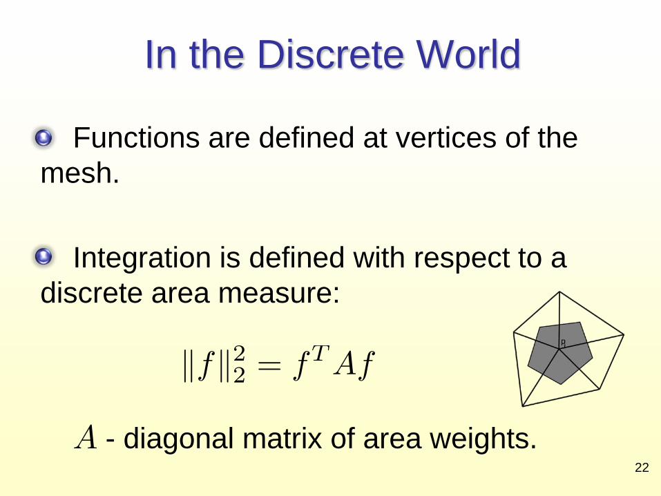
In the Discrete World

Functions are defined at vertices of the mesh. Integration is defined with respect to a discrete area measure:

- diagonal matrix of area weights.

22

An Eigenvalue Problem

Computing the eigenfunctions of the Laplacian reduces to solving the eigenvalue problem:

Both C and A are sparse positive semidefinite.

Number of triangles

Computation time (in s)

5000 0.65 25000 2.32 50868 3.6 105032 10

Computing 100 eigenpairs 23

24

Functional Maps and Shape Differences

Functional Maps (a.k.a. Operators)

25

[M. Ovsjanikov, M. Ben-Chen, J. Solomon, A. Butscher, L. G., Siggraph ’12]

A Contravariant Functor

26

An “attribute transfer’’ operator

Inversion is possible (F2F → P2P)

P2P → F2F

Starting from a Regular Map

27 lion → cat

Attribute Transfer via Pull-Back

28 cat → lion

The Operator View of Maps

Functions on cat are transferred to lion using F

F is a linear operator (matrix)

from cat to lion

29

Functional Map Representation

30

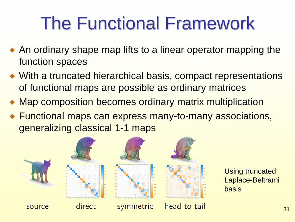
The Functional Framework An ordinary shape map lifts to a linear operator mapping the function spaces With a truncated hierarchical basis, compact representations of functional maps are possible as ordinary matrices Map composition becomes ordinary matrix multiplication Functional maps can express many-to-many associations, generalizing classical 1-1 maps

31

Using truncated Laplace-Beltrami basis

Estimating the Mapping Matrix Suppose we don’t know C. However, we expect a pair of functions and to correspond. Then, C must be s.t.

where

32

A Shape Mapping Tool: Descriptors for Points and Parts

33

For shapes, there are many descriptors with various types of invariances

Spin Images: [Johnson, Hebert ’99]

Shape Contexts: [Belongie et al. ’00, Frome et al. ’04]

Wave Kernel Signatures (WKS): [Aubry et. al. ‘11]

Heat Kernel Signatures (HKS): [Sun, Ovsjanikov, G. ’08]]

Rigid invariance (extrinsic)

Isometric invariance (intrinsic)

Estimating the Mapping Matrix

Suppose we don’t know C. However, we expect a pair of functions and to correspond. Then, C must be s.t.

where

Given enough pairs in correspondence, we can recover C through a linear least squares system. 34

Function Preservation Constraints

Suppose we don’t know C. However, we expect a pair of functions and to correspond. Then, C must be s.t.

Function preservation constraint is quite general and includes:

Texture preservation.

Descriptor preservation (e.g. Gaussian curvature, spin images, HKS, WKS).

Landmark correspondences (e.g. distance to the point).

Part correspondences (e.g. indicator function).

35

Commutativity Constraints

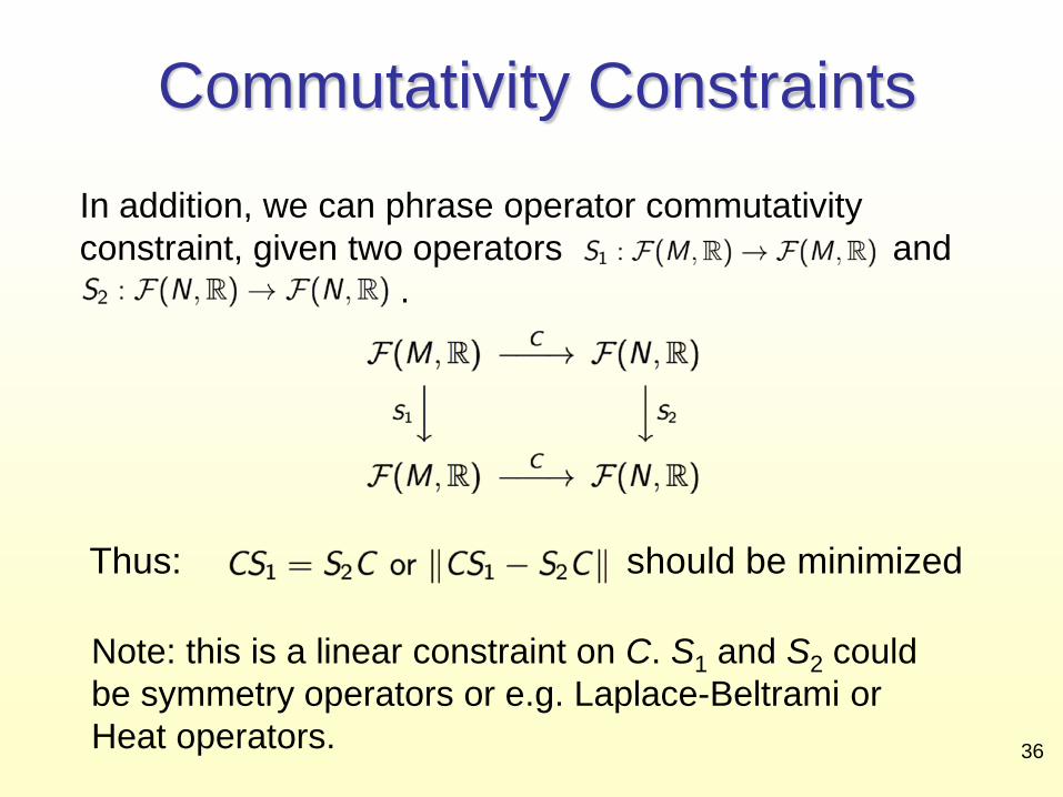
In addition, we can phrase operator commutativity constraint, given two operators and .

Thus: should be minimized

Note: this is a linear constraint on C. S1 and S2 could be symmetry operators or e.g. Laplace-Beltrami or Heat operators.

36

Regularization

Lemma 1:

The mapping is isometric, if and only if the functional map matrix commutes with the Laplacian:

37

Regularization

Lemma 2:

The mapping is locally volume preserving, if and only if the functional map matrix is orthonormal:

38

Regularization

Lemma 3:

If the mapping is conformal if and only if:

Using these regularizations, we get a very efficient shape matching method.

39

Map Estimation Quality

40 Roughly 10 probe functions + 1 part correspondence

App: Shape Differences

41

[R. Rustamov, M. Ovsjanikov, O. Azercot, M. Ben-Chen, F. Chazal, L.G. Siggraph ’13]

vs.

Understanding Intrinsic Distortions

Where and how are shapes different, locally and globally, irrespective of their embedding

42

Area distortion Conformal distortion

Classical Approach to Relating Shapes

To measure distortions induced by a map, we track how inner products of vectors change after transporting

Challenges: • point-wise information only, hard

to aggregate • noisy

Riemann

43

A Functional View of Distortions

To measure distortions induced by a map, track how inner products of vectors change after transporting.

To measure distortions induced by a

map, track how inner products of functions change after transporting.

Riemann

44

The Art of Measurement A metric is defined by a functional inner product So we can compare M and N by comparing

45

Riemann

M

F N

The functional map F transports these functions to N, where we repeat this measurement with the inner product hN(F(f),F(g))

Measurement Discrepancies

after before

Both can be considered as inner products on the cat 46

The Universal Compensator

There exists a linear operator such that

1907 1909

Comptes Rendus Hebdomadaires des Séances de l'Académie des Sciences de Paris

Frigyes Riesz

Riesz Representation Theorem

47

Area-Based Shape Difference:

48

A Small Example of V

49

Conformal Shape Difference: R Consider a different inner-product of functions ... get information about conformal distortion

The choice of inner product should be driven by the application at hand.

50

Shape Differences in Collections

51

Comparing Differences I

…

52

Intrinsic Shape Space

…

Area Conformal 1 8

64 57

28 29

36 37

53

Area Conformal

13

4

16

1

21 24

Intrinsic Shape Space

54

Localized Comparisons

supported in RoI

…

ROI

½ : M ! R

D1½ to D2½

55

Exaggeration of Difference in RoI

56

Comparing Differences II

57

Analogies: D relates to C as B relates to A

A B

C D

output

D = C + (B – A) hands raised up

58

Analogies: D relates to C as B relates to A

Entire SCAPE

D

output

…

A B

C

Input

F

59

Shape Analogies A B A

C D

B

output

C D

output

60

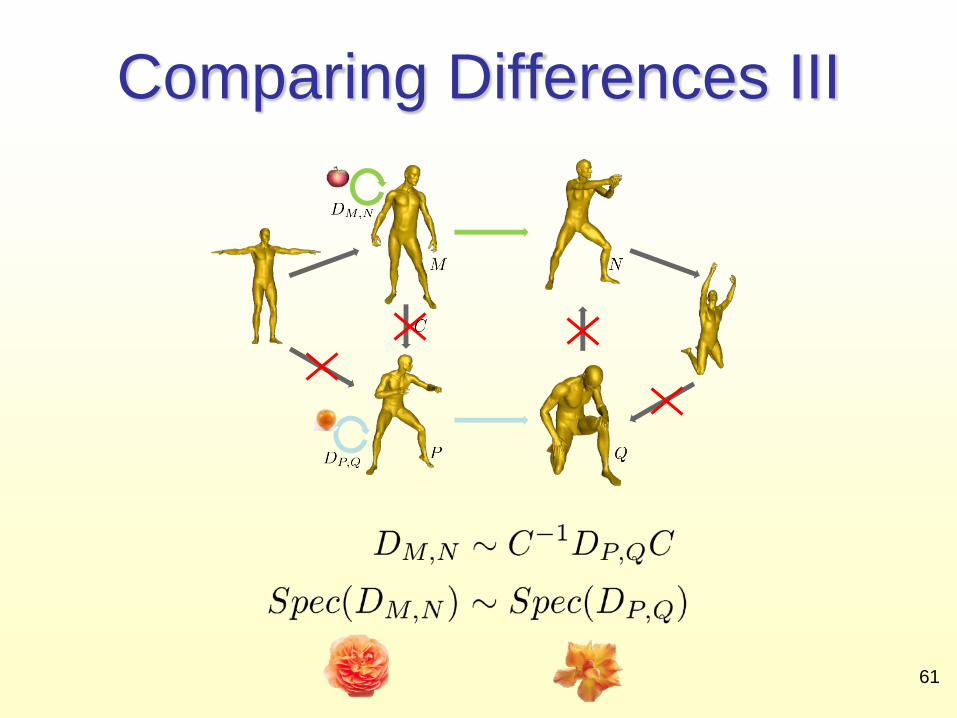
Comparing Differences III

61

Aligning Disconnected Collections

First Collection Second Collection

62

Complete graph

… …

Complete graph

Aligning Disconnected Collections

63

Aligning, Without “Crossing the River”

64

Comparing the differences is sometimes easier than comparing the originals

65

Networks of Shapes and Images

Maps vs. Distances/Similarities Networks vs. Graphs

66

A B C

Map Networks for Related Data

67

Maps vs. similarities

Networks of “samenesses”

68

Saunders MacLane

Samuel Eilenberg

The Information is in the Maps

Herni Cartan

A Functorial View of Data

Homological Algebra 1956

Yes, But With a Statistical Flavor

Yes, straight out of the playbook of homological algebra / algebraic topology But, the maps

are not given by canonical constructions they have to be estimated and can be noisy the network acts as a regularizer … commutativity still very important imperfections of commutativity in function transport convey valuable information: consistency vs. variability – “curvature” in shape space

69

Cycle-Consistency ≡ Low-Rank

In a map network, commutativity, path-invariance, or cycle-consistency are equivalent to a low rank or semidefiniteness condition on a big mapping matrix Conversely, such a low-rank condition can be used to regularize functional maps

70

Exploitation of the Wisdom in a Collection

71

Emergence of Shared Structure

72

Plato’s cow

Entity Extraction in Images

Task: jointly segment a set of related images same object, different viewpoints/scales: similar objects of the same class:

Benefits and challenges: Images can provide weak supervision for each other But exactly how should they help each other? How to deal with clutter and irrelevant content?

[F. Wang, Q. Huang, L. G., ICCV ’13]

73

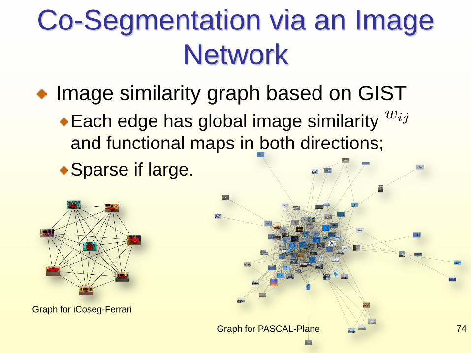
Co-Segmentation via an Image Network

Image similarity graph based on GIST Each edge has global image similarity and functional maps in both directions; Sparse if large.

74

Graph for iCoseg-Ferrari

Graph for PASCAL-Plane

The Pipeline

a) Superpixel graph representation of images

b) Functions over these graphs expressed in terms of the eigenvectors of the graph Laplacian

c) Estimation of functional maps along network edges such that • Image features are preserved • Maps are cycle consistent in the network

d) The “cow functions” emerge as the most consistently transported set 75

Superpixel Representation

Over-segment images into super-pixels Build a graph on super-pixels

Nodes: super-pixels Edges weighted by length of shared boundary

76

Encoding Functions over Graphs

Basis of functional space : First M Laplacian eigenfunctions of the graph

Reconstruct any function with small error (M=30)

Binary indicator function Reconstructed function Thresholded reconstructed function

Reconstruction error 77

Functional map: A linear map between functions in two functional spaces Can be recovered by a set of probe functions

Joint Estimation of Functional Maps, I

78

Joint Estimation of Functional Maps, I

Recover functional maps by aligning image features:

Features (probe functions) for each super-pixel:

average RGB color, 3-dimensional; 64 dimensional RGB color histogram; 300-dimensional bag-of-visual-words.

79

Joint Estimation of Functional Maps, II

Regularization term:

Correspond bases of similar spectra Enforce sparsity of map

Map with regularization Map without regularization

Λi, Λj diagonal matrices of Laplacian eigenvalues

80

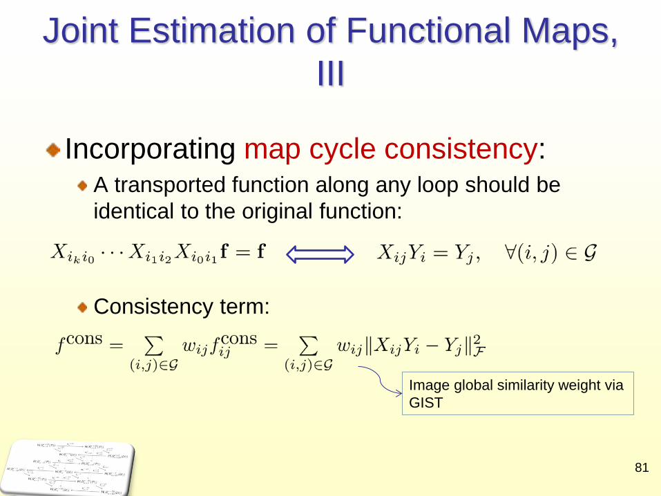
Joint Estimation of Functional Maps, III

Incorporating map cycle consistency: A transported function along any loop should be identical to the original function: Consistency term:

Image global similarity weight via GIST

81

Joint Estimation of Functional Maps, III

Plato’s allegory of the cave

82 X 30x30, Y 30x20

Joint Estimation of Functional Maps, IV

Overall optimization Alternating optimization:

Fix Y, solve X Independent QP problems

Fix X, solve Y Eigenvalue problem

83

Consistency Matters

84

Source image

Target image

Without cycle consistency

With cycle consistency

RGB Transport under FMaps

85

Part Transport As Well

Gymnastics in iCoseg

upper body and lower body

86

Generating Consistent Segmentations

Two objectives for segmentation functions consistent under functional map transportation

agreement with normalized cut scores:

Joint optimization:

Easy to incorporate labeled images with ground truth segmentation

Eigen-decomposition problem

consistent

87

Experiments

iCoseg dataset Very similar or the same object in each class; 5~10 images per class.

MSRC dataset Similar objects in each class; ~30 images per class.

PASCAL data set Retrieved from PASCAL VOC 2012 challenge; All images with the same object label; Larger scale; Larger variability.

88

Kuettel’12 (Supervised) Unsupervised Fmaps

Image+transfer Full model

87.6 91.4 90.5

Class Joulin ’10

Rubio ’12

Vicente ’11

Fmaps -uns

Alaska Bear 74.8 86.4 90.0 90.4

Red Sox Players 73.0 90.5 90.9 94.2

Stonehenge1 56.6 87.3 63.3 92.5

Stonehenge2 86.0 88.4 88.8 87.2

Liverpool FC 76.4 82.6 87.5 89.4

Ferrari 85.0 84.3 89.9 95.6

Taj Mahal 73.7 88.7 91.1 92.6

Elephants 70.1 75.0 43.1 86.7

Pandas 84.0 60.0 92.7 88.6

Kite 87.0 89.8 90.3 93.9

Kite panda 73.2 78.3 90.2 93.1

Gymnastics 90.9 87.1 91.7 90.4

Skating 82.1 76.8 77.5 78.7

Hot Balloons 85.2 89.0 90.1 90.4

Liberty Statue 90.6 91.6 93.8 96.8

Brown Bear 74.0 80.4 95.3 88.1

Average 78.9 83.5 85.4 90.5

iCoseg data set New unsupervised method

Mostly outperforms other unsupervised methods Sometimes even outperforms supervised methods Supervised input is easily added and further improves the results

Supervised method

89

MSRC Unsupervised performance comparison

Supervised performance comparison

Class N Joulin ’10

Rubio ’12

Fmaps -uns

Cow 30 81.6 80.1 89.7

Plane 30 73.8 77.0 87.3

Face 30 84.3 76.3 89.3

Cat 24 74.4 77.1 88.3

Car(front) 6 87.6 65.9 87.3

Car(back) 6 85.1 52.4 92.7

Bike 30 63.3 62.4 74.8

Class Vicente ’11

Kuettel ’12

Fmaps -s

Cow 94.2 92.5 94.3

Plane 83.0 86.5 91.0

Car 79.6 88.8 83.1

Sheep 94.0 91.8 95.6

Bird 95.3 93.4 95.8

Cat 92.3 92.6 94.5

Dog 93.0 87.8 91.3

• PASCAL Class N L Kuettel

’12 Fmaps

-s Fmaps

-uns

Plane 178 88 90.7 92.1 89.4

Bus 152 78 81.6 87.1 80.7

Car 255 128 76.1 90.9 82.3

Cat 250 131 77.7 85.5 82.5

Cow 135 64 82.5 87.7 85.5

Dog 249 121 81.9 88.5 84.2

Horse 147 68 83.1 88.9 87.0

Sheep 120 63 83.9 89.6 86.5

• New method mostly outperforms the state-of-the-art techniques in both supervised and unsupervised settings

90

iCoseg: 5 images per class are shown

91

iCoseg: 5 images per class are shown

92

iCoseg: 5 images per class are shown

93

iCoseg: 5 images per class are shown

94

MSRC: 5 images per class are shown

95

MSRC: 5 images per class are shown

96

PASCAL: 10 images per class are shown

97

PASCAL: 10 images per class are shown

98

PASCAL: 10 images per class are shown

99

PASCAL: 10 images per class are shown

100

Multi-Class Co-Segmentation

Input: A collection of N images sharing M objects Each image contains a subset of the objects

Output Discovery of what objects appear in each image Their pixel-level segmentation 101

[F. Wang, Q. Huang, M. Ovsjanikov, L. G., CVPR’14]

Framework

102

Partial cycle consistency:

Consistent Functional Maps

103

Latent functions: Discrete variables: Relationship: Consistency:

Consistent Functional Maps

104

YiDiag(zi) = Yi

zi = fzil 2 f0;1g;1 · l · Lg

XijY i = Y jDiag(zi); (i; j) 2 E:

Y i = (yi1; ¢ ¢ ¢ ;yiL)

The consistency regularization Overall optimization

Consistent Functional Maps

105

fcons =¹X

(i;j)2EkXijYi ¡YjDiag(zi)k2

+ °NX

i=1

kYi ¡YiDiag(zi)k2;

fX?ijg = argminXij

0

@¹fcons +P

(i;j)2Efpair

1

A

Framework

106

Initialization

Solve for consistent segmentation with ALL images together Pick the first M eigenvectors Each object class is initialized as:

fseg =1

jGjX

(i;j)2GkXijsik ¡ sjkk2F +

°

N

NX

i=1

sTikLisik

= skLsk;

Ck = fi; s.t. ksikk ¸ maxi

ksik=2g

107

Continuous Optimization

Optimize segmentations in each object class Consistent with functional maps Align with segmentation cues Mutually exclusive

minsik;i2Ck

MX

k=1

X

(i;j)2E\(Ck£Ck)kXijsik ¡ sjkk2

+ °X

l 6=k

X

i2Ck\Cl(sTilsik)

2 + ¹MX

k=1

X

i2CksTikLisik

subject toX

i2Ckksikk2 = jCkj; 1 · k · K:

108

Combinatorial Optimization

Expand each object class by propagating segmentations to other images

maxsik

1

jN (i) \ CkjX

j2N (i)\Ck(sTikXjisjk)

2

¡ °X

l 6=k;i2Cl(sTiksil)

2 ¡ ¹sTikLisik

subject to ksikk2 = 1

109

Alternating between: Continuous optimization:

Optimal segmentation functions in each class Combinatorial optimization:

Class assignment by propagating segmentation functions

Optimizing Segmentation Functions

110

Optimizing Segmentation Functions

More images will be included in each object class

• Segmentation functions are improved during iterations

111

Experimental Results

Accuracy Intersection-over-union Find the best one-to-one matching between each cluster and each ground-truth object.

Benchmark datasets MSRC: 30 images, 1 class (degenerated case); FlickrMFC data set: 20 images, 3~6 classes PASCAL VOC: 100~200 images, 2 classes

112

Experimental Results

class N M Kim’12 Kim’11 Joulin ’10

Mukherjee ’11

Ours

Apple 20 6 40.9 32.6 24.8 25.6 46.6

Baseball 18 5 31.0 31.3 19.2 16.1 50.3

butterfly 18 8 29.8 32.4 29.5 10.7 54.7

Cheetah 20 5 32.1 40.1 50.9 41.9 62.1

Cow 20 5 35.6 43.8 25.0 27.2 38.5

Dog 20 4 34.5 35.0 32.0 30.6 53.8

Dolphin 18 3 34.0 47.4 37.2 30.1 61.2

Fishing 18 5 20.3 27.2 19.8 18.3 46.8

Gorilla 18 4 41.0 38.8 41.1 28.1 47.8

Liberty 18 4 31.5 41.2 44.6 32.1 58.2

Parrot 18 5 29.9 36.5 35.0 26.6 54.1

Stonehenge 20 5 35.3 49.3 47.0 32.6 54.6

Swan 20 3 17.1 18.4 14.3 16.3 46.5

Thinker 17 4 25.6 34.4 27.6 15.7 68.6

Average - - 31.3 36.3 32.0 25.1 53.1

113 Performance comparison on the MFCFlickr dataset

class N NCut MNcut Ours

Bike + person 248 27.3 30.5 40.1

Boat + person 260 29.3 32.6 44.6

Bottle + dining table 90 37.8 39.5 47.6

Bus + car 195 36.3 39.4 49.2

bus + person 243 38.9 41.3 55.5

Chair + dining table 134 32.3 30.8 40.3

Chair + potted plant 115 19.7 19.7 22.3

Cow + person 263 30.5 33.5 45.0

Dog + sofa 217 44.6 42.2 49.6

Horse + person 276 27.3 30.8 42.1

Potted plant + sofa 119 37.4 37.5 40.7

Performance comparison on the PASCAL-multi dataset

class N Joulin’10 Kim’11 Mukherjee’11 Ours

Bike 30 43.3 29.9 42.8 51.2

Bird 30 47.7 29.9 - 55.7

Car 30 59.7 37.1 52.5 72.9

Cat 24 31.9 24.4 5.6 65.9

Chair 30 39.6 28.7 39.4 46.5

Cow 30 52.7 33.5 26.1 68.4

Dog 30 41.8 33.0 - 55.8

Face 30 70.0 33.2 40.8 60.9

Flower 30 51.9 40.2 - 67.2

House 30 51.0 32.2 66.4 56.6

Plane 30 21.6 25.1 33.4 52.2

Sheep 30 66.3 60.8 45.7 72.2

Sign 30 58.9 43.2 - 59.1

Tree 30 67.0 61.2 55.9 62.0 Performance comparison on the MSRC dataset

Apple + picking

Baseball + kids

Butterfly + blossom

114

Apple + picking (red: apple bucket; magenta: girl in red; yellow: girl in blue; green: baby; cyan: pump

Baseball + kids (green: boy in black; blue: boy in grey; yellow: coach.)

Butterfly + blossom (green: butterfly in orange; yellow: butterfly in yellow; cyan: red flowe

115

Cheetah + Safari

Cow + pasture

Dog + park

Dolphin + aquarium

116

Cheetah + Safari (red: cheetah; yellow: lion; magenta: monkey.)

Cow + pasture (red: black cow; green: brown cow; blue: man in blue.)

Dog + park (red: black dog; green: brown dog; blue: white dog.)

Dolphin + aquarium (red: killer whale; green: dolphin.)

117

Fishing + Alaska

Gorilla + zoo

Liberty + statue

Parrot + zoo

118

Fishing + Alaska (blue: man in white; green: man in gray; magenta: woman in gray; yellow: salmon.

Gorilla + zoo (blue: gorilla; yellow: brown orangutan)

Liberty + statue (blue: empire state building; green: red boat; yellow: liberty statue.)

Parrot + zoo (red: hand; green: parrot in green; blue: parrot in red.)

119

Stonehenge

Swan + zoo

Thinker + Rodin

120

Stonehenge (blue: cow in white; yellow: person; magenta: stonehenge.)

Swan + zoo (blue: gray swan; green: black swan.)

Thinker + Rodin (red: sculpture Thinker; green: sculpture Venus; blue: Van Gogh.)

121

The Network is the Abstraction

122

Plato’s cow

The Network is the Abstraction

123

Plato’s cow

The Network is the Abstraction

124

a co-limit

Mosaicing or SLAM at the Level of Functions

125 robotics.ait.kyushu-u.ac.jp

http://www.cs.cmu.edu/afs/cs.cmu.edu/academic/class/15463-f08/www/proj4/www/gme/

126

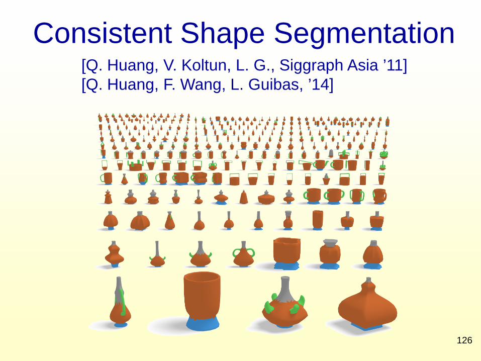
Consistent Shape Segmentation [Q. Huang, V. Koltun, L. G., Siggraph Asia ’11] [Q. Huang, F. Wang, L. Guibas, ’14]

First Build a Network

127

Use the D2 shape descriptor and connect each shape to its nearest neighbors

distance histogram

Start From Noisy Shape Descriptor Correspondences

128

Lift to functional form

Ci Di

Algebraic Dependencies Between Maps

Cycle consistency or closure

129 consistent cycles inconsistent cycles

Cycle Consistency for Partial Maps

The functional map network G = (V ; E) is cycle-consistent, if there exists or-thogonal bases Bi =

¡bi1; ¢ ¢ ¢ ;bidim(Fi)

¢for each functional space Fi so that

Xi1i2bi1j = bi2j0 or 0 81 · j · dim(Fi1); 9j0;

Xiki1 ¢ ¢ ¢Xi1i2bi1j = bi1j or 0 8 1 · j · dim(Fi1);(i1 ¢ ¢ ¢ iki1) 2 L(G);

where L(G) denotes the set of all loops of G.

130

Such basis functions could, for example, be indicator functions of common shape parts or segments

Equivalent Formulation There exist row-orthogonal matrices

such that where is the Moore-Penrose pseudoinverse of . The are maps from the to multiple latent spaces, along which some sub-collections of the shapes agree. The orthogonality of the allows efficient optimization.

131

Yi = (yi1; ¢ ¢ ¢ ;yiL)T 2 RL£dim(Fi); 1 · i · N

Xij = Y +j Yi; 8(i; j) 2 G

Abstractions Emerge from he Network

Cycle Consistent Diagram

F6

F1

F2

F3

F4

F5

X12

X54X24

132

Abstraction – Colimit

Colimits glue parts together to make a whole Saunders MacLane

Samuel Eilenberg

F6

F1

F2

F3

F4

F5

X12

X54X24

lim¡!Fi =G

i

FiÁ

»133

Abstraction – Approximate Colimit

Find projections that “play well” with maps on network edges,

or

F6

F1

F2

F3

F4

F5

X12

X54X24

lim¡!Fi =G

i

FiÁ

» YjXij ¼ Yi Xij ¼ Y +j Yi

Y1

Y2Y3 Y4 Y5

Y6

134

Low-Rank Factorization

135

X :=

0

B@X11 ¢ ¢ ¢ XN1

.... . .

...X1N ¢ ¢ ¢ XNN

1

CA =

0

B@Y +

1...

Y +N

1

CA¡

Y1 ¢ ¢ ¢ YN¢

:

The total dimensions of the Yi is much less than the dimension of X. In a map network, commutativity, path-invariance, or cycle-consistency are equivalent to a low rank or semidefiniteness condition on the big mapping matrix X.

The Pipeline

136

Original shapes with noisy maps

Cleaned up maps Consistent basis functions extracted

Step 1 Step 2

Joint Map Optimization

Step 1: Convex low-rank recovery using robust PCA – we minimize over all X Step 2: Perturb the above X to force the factorization

137

X? = ¸kXk? + minX

X

(i;j)2G

kXijCij ¡Dijk2;1

X

1·i;j·N

kX?ij ¡ Y +

j Yik2F + ¹

NX

i=1

X

1·k<l·L

(yTikyil)2

kXk? =P

i ¾i(X)trace norm

kAk2;1 =P

i k~aik

The Yi give us the desired latent spaces

Dual ADMM

Non-linear least squares Gauss-Newton descent

Hierarchical Scaling

138

Multiple abstraction levels

Route maps via the abstractions

Consistent Shape Segmentation

139 Via 2nd order MRF on each shape independently

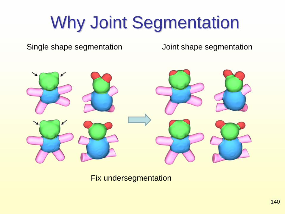
Why Joint Segmentation Single shape segmentation

Fix undersegmentation

Joint shape segmentation

140

Why Joint Segmentation Single shape segmentation Joint shape segmentation

Fix oversegmentation

141

Segmentation Results

142

Shape Classification via RoI Shape Differences

143

Shape Inter-/Extra-polation

144

Co-Detection of Features and Communities

145

cats and lions

by animal by pose

Networks of Shapes and Images

146

Depth Inference from a Single Image

147

single image shape network inferred depth

+ →

148

149

150

151

Conclusion: Functoriality Classical “vertical” view of data analysis:

Signals to symbols from features, to parts, to semantics …

A new “horizontal” view based on peer-to-peer signal relationships

so that semantics emerge from the network 152

Functions over data

Maps between data

Networks of data sets

Acknowledgements

Collaborators: Current students: Justin Solomon, Fan Wang Current and past postdocs: Adrian Butscher, Qixing Huang, Raif Rustamov Senior: Mirela Ben-Chen, Frederic Chazal, Maks Ovsjanikov

Sponsors:

153

Exercises I 1. Given two shapes, a functional map between them: (a) relates how the two objects are used by humans (their function) (b) transports functions defined over one shape to functions defined over the other shape (c) describes point-to-point correspondences between the shapes (d) is a map of the landscape defined by functions over the product space of the two shapes 2. A shape difference operator associated with a map F from shape M to shape N: (a) is a list of all ways in which the two shapes are different (b) is a procedure that can transform or morph shape M into shape N (c) is a linear map of functions from M to M that compensates for distortions introduced by the map F during function transport, as measured by the metrics on the two shapes (d) highlights the areas on M and N where the two shapes differ the most

154

Exercises II 3. Consider a complete network of n images. For each ordered pair of images i and j we have a functional map F_{ij} between them. Assume that F_{ji} = F_{ij}^{-1}. If the network is fully consistent (so all cycles close perfectly), how many of the maps F_{ij} are independent? in other words, what is the smallest number of maps that need to be specified, so that all others can be generated from them? (a) n-1 (b) n (c) n \log n (d) n(n-1)/4

155

Exercises III 4. When a network of images or shapes is connected by functional maps that are only partially consistent, a function transported by the network around a cycle back to its original domain: (a) must come back unaltered, or as 0 (c) must remain unaltered the vast majority of the time, but a small percentage of exceptions is allowed (d) functions can be grouped into clusters, so that after transport a function must come back as a member of it own cluster (d) the function may be altered, but its basic structure, as measured by topological persistence, must be preserved. 156

Much More to Do …

Get in touch, if interested in projects in this area: guibas@cs.stanford.edu Soon a website, www.mapnets.org IAS Hong Kong Workshop, April 2015 Dagstuhl Seminar, Fall 2015

157

158

A Network of MOOC Homeworks