lecture 6 : discrete random variables and probability...

Lecture 6 : Discrete Random Variables and ProbabilityDistributions

0/ 31

1/ 31

Go to “BACKGROUND COURSE NOTES” at the end of my web page anddownload the file distributions.Today we say goodbye to the elementary theory of probability and start Chapter3. We will open the door to the application of algebra to probability theory byintroduction the concept of “random variable”.

Lecture 6 : Discrete Random Variables and Probability Distributions

2/ 31

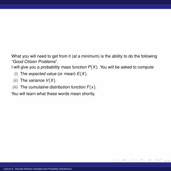
What you will need to get from it (at a minimum) is the ability to do the following“Good Citizen Problems”.I will give you a probability mass function P(X). You will be asked to compute

(i) The expected value (or mean) E(X).

(ii) The variance V(X).

(iii) The cumulative distribution function F(x).

You will learn what these words mean shortly.


3/ 31

Mathematical DefinitionLet S be the sample space of some experiment (mathematically a set S with aprobability measure P). A random variable X is a real-valued function on S.

Intuitive IdeaA random variable is a function, whose values have probabilities attached.

Remark

To go from the mathematical definition to the “intuitive idea” is tricky and notreally that important at this stage.


4/ 31

The Basic ExampleFlip a fair coin three times so

S = {HHH, HHT , HTH, HTT , THH, THT , TTH, TTT }

Let X be function on X given by

X = number of heads

so X is the function given by

{HHH, HHT , HTH, HTT , THH, THT , TTH, TTT }↓ ↓ ↓ ↓ ↓ ↓ ↓ ↓

3 2 2 1 2 1 1 0

What areP(X = 0), P(X = 3), P(X = 1), P(X = 2)


5/ 31

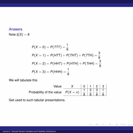
AnswersNote ](S) = 8

P(X = 0) = P(TTT) =18

P(X = 1) = P(HTT) + P(THT) + P(TTH) =38

P(X = 2) = P(HHT) + P(HTH) + P(THH) =38

P(X = 3) = P(HHH) =18

We will tabulate this

Value X 0 1 2 3

Probability of the value P(X = x)18

38

38

18

Get used to such tabular presentations.


6/ 31

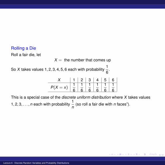
Rolling a DieRoll a fair die, let

X = the number that comes up

So X takes values 1, 2, 3, 4, 5, 6 each with probability16

.

X 1 2 3 4 5 6

P(X = x)16

16

16

16

16

16

This is a special case of the discrete uniform distribution where X takes values

1, 2, 3, . . . , n each with probability1n

(so roll a fair die with n faces”).


7/ 31

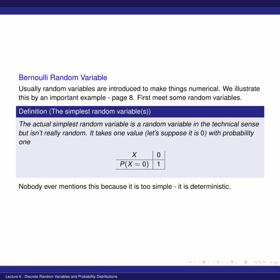
Bernoulli Random VariableUsually random variables are introduced to make things numerical. We illustratethis by an important example - page 8. First meet some random variables.

Definition (The simplest random variable(s))

The actual simplest random variable is a random variable in the technical sensebut isn’t really random. It takes one value (let’s suppose it is 0) with probabilityone

X 0P(X = 0) 1

Nobody ever mentions this because it is too simple - it is deterministic.


8/ 31

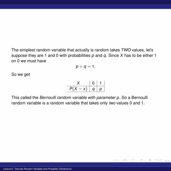
The simplest random variable that actually is random takes TWO values, let’ssuppose they are 1 and 0 with probabilities p and q. Since X has to be either 1on 0 we must have

p + q = 1.

So we get

X 0 1P(X = x) q p

This called the Bernoulli random variable with parameter p. So a Bernoullirandom variable is a random variable that takes only two values 0 and 1.


9/ 31

Where do Bernoulli random variables come from?We go back to elementary probability.

Definition

A Bernoulli experiment is an experiment which has two outcomes which we call(by convention) “success” S and failure F.

Example

Flipping a coin. We will call a head a success and a tail a failure.

Z Often we call a “success” something that is in fact for from an actual success-e.g., a machine breaking down.


10/ 31

In order to obtain a Bernoulli random variable if we first assign probabilities to Sand F by

P(S) = p and P(F) = q

so again p + q = 1.Thus the sample space of a a Bernoulli experiment will be denoted S (note thatthat the previous caligraphic S is different from Roman S) and is given by

S = {S,F}.

We then obtain a Bernoulli random variable X on S by defining

X(S) = 1 and X(F) = 0

so P(X = 1) = P(S) = p and P(X = 0) = P(F) = q.


11/ 31

Discrete Random Variables

Definition

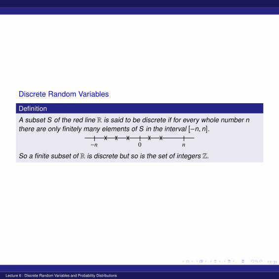
A subset S of the red line R is said to be discrete if for every whole number nthere are only finitely many elements of S in the interval [−n, n].

0

So a finite subset of R is discrete but so is the set of integers Z.


12/ 31

Remark

The definition in the text on page 98 is wrong. The set of rational numbers Q iscountably infinite but is not discrete. This is not important for this course but Ifind it almost unbelievablel that the editors of this text would allow such an errorto run through nine editions of the text.

Definition

A random variable is said to be discrete if its set of possible values is a discreteset.

A possible value means a value x0 so that P(X = x0) , 0.


13/ 31

Definition

The probability mass function (abbreviated pmf) of a discrete random variable Xis the function pX defined by

pX(x) = P(X = x)

We will often write p(x) instead of PX(x).Note

(i) P(x) ≥ 0

(ii)∑

all possibleX

P(x) = 1

(iii) P(x) = 0 for all X outside a countable set.


14/ 31

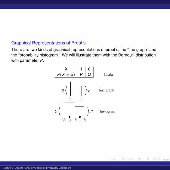
Graphical Representations of Proof’sThere are two kinds of graphical representations of proof’s, the “line graph” andthe “probability histogram”. We will illustrate them with the Bernoulli distributionwith parameter P.

X 1 0P(X = x) P Q table

0 1

line graph

0 1

histogram


15/ 31

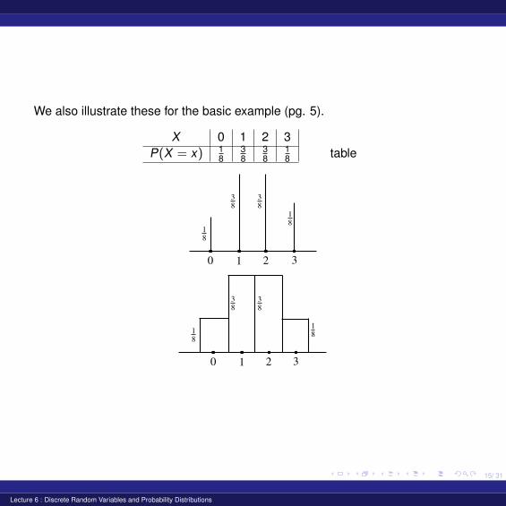
We also illustrate these for the basic example (pg. 5).

X 0 1 2 3P(X = x) 1

838

38

18 table

0 1 2 3

0 1 2 3


16/ 31

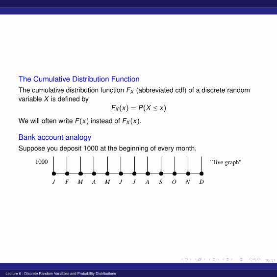
The Cumulative Distribution FunctionThe cumulative distribution function FX (abbreviated cdf) of a discrete randomvariable X is defined by

FX(x) = P(X ≤ x)

We will often write F(x) instead of FX(x).

Bank account analogySuppose you deposit 1000 at the beginning of every month.

1000 ``live graph''


17/ 31

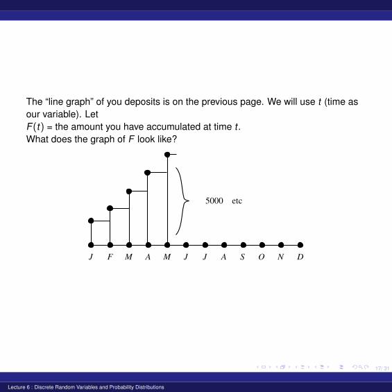
The “line graph” of you deposits is on the previous page. We will use t (time asour variable). LetF(t) = the amount you have accumulated at time t .What does the graph of F look like?

5000 etc


18/ 31

It is critical to observe that whereas the deposit function on page 15 is zero forall real numbers except 12 the cumulation function is never zero between 1 and∞. You would be very upset if you walked into the bank on July 5th and they toldyou your balance was zero - you never took any money out. Once your balancewas nonzero it was never zero thereafter.


19/ 31

Back to ProbabilityThe cumulative distribution F(x) is “the total probability you have accumulatedwhen you get to x”. Once it is nonzero it is never zero again (P(x) ≥ 0 means“you never take any probability out”).To write out F(x) in formulas you will need several (many) formulas. Thereshould never be EQUALITIES in you formulas only INEQUALITIES.


20/ 31

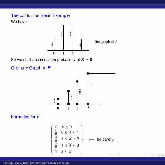
The cdf for the Basic ExampleWe have

0 1 2 3

line graph of

So we start accumulation probability at X = 0

Ordinary Graph of F

0 1 2 3

1

Formulas for F

0 X ≤ 018 0 ≤ X < 148 1 ≤ X < 278 1 ≤ X < 3

1 3 ≤ X

←− be careful


21/ 31

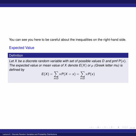
You can see you here to be careful about the inequalities on the right-hand side.

Expected Value

Definition

Let X be a discrete random variable with set of possible values D and pmf P(x).The expected value or mean value of X denote E(X) or µ (Greek letter mu) isdefined by

E(X) =∑x∈D

×P(X = x) =∑x∈D

×P(x)


22/ 31

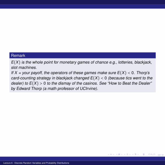
Remark

E(X) is the whole point for monetary games of chance e.g., lotteries, blackjack,slot machines.If X = your payoff, the operators of these games make sure E(X) < 0. Thorp’scard-counting strategy in blackjack changed E(X) < 0 (because tics went to thedealer) to E(X) > 0 to the dismay of the casinos. See “How to Beat the Dealer”by Edward Thorp (a math professor of UCIrvine).


23/ 31

Examples

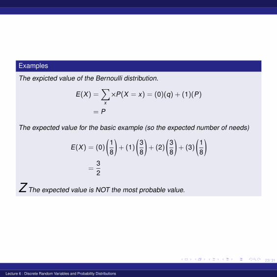
The expicted value of the Bernoulli distribution.

E(X) =∑

x

×P(X = x) = (0)(q) + (1)(P)

= P

The expected value for the basic example (so the expected number of needs)

E(X) = (0)(18

)+ (1)

(38

)+ (2)

(38

)+ (3)

(18

)=

32

Z The expected value is NOT the most probable value.


24/ 31

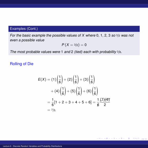
Examples (Cont.)

For the basic example the possible values of X where 0, 1, 2, 3 so 3/2 was noteven a possible value

P (X = 3/2) = 0

The most probable values were 1 and 2 (tied) each with probability 3/8.

Rolling of Die

E(X) = (1)(16

)+ (2)

(16

)+ (3)

(16

)+ (4)

(16

)+ (5)

(16

)+ (6)

(16

)=

16[1 + 2 + 3 + 4 + 5 + 6] =

1

�6��(7)(6)

2= 7/3.


25/ 31

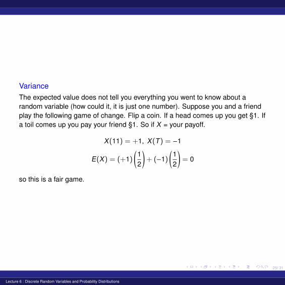
VarianceThe expected value does not tell you everything you went to know about arandom variable (how could it, it is just one number). Suppose you and a friendplay the following game of change. Flip a coin. If a head comes up you get §1. Ifa toil comes up you pay your friend §1. So if X = your payoff.

X(11) = +1, X(T) = −1

E(X) = (+1)(12

)+ (−1)

(12

)= 0

so this is a fair game.


26/ 31

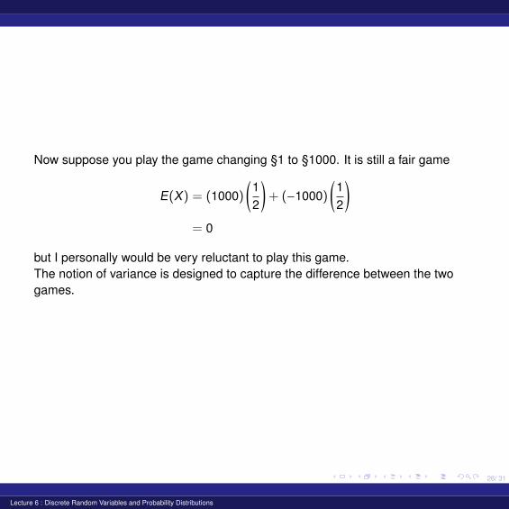
Now suppose you play the game changing §1 to §1000. It is still a fair game

E(X) = (1000)(12

)+ (−1000)

(12

)= 0

but I personally would be very reluctant to play this game.The notion of variance is designed to capture the difference between the twogames.


27/ 31

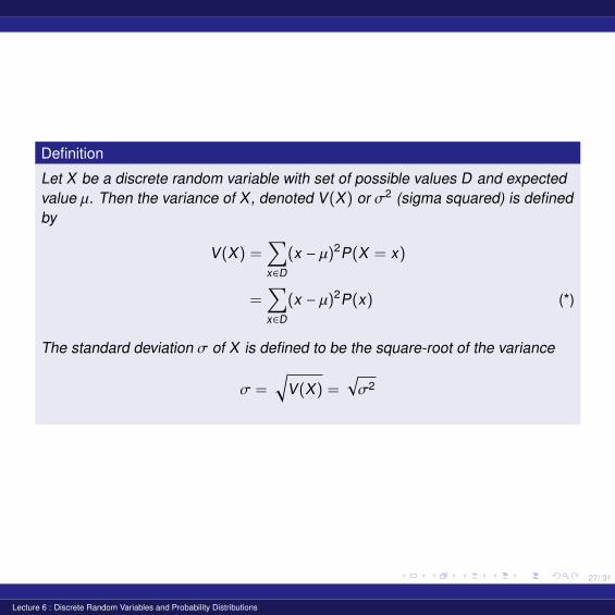
Definition

Let X be a discrete random variable with set of possible values D and expectedvalue µ. Then the variance of X, denoted V(X) or σ2 (sigma squared) is definedby

V(X) =∑x∈D

(x − µ)2P(X = x)

=∑x∈D

(x − µ)2P(x) (*)

The standard deviation σ of X is defined to be the square-root of the variance

σ =√

V(X) =√σ2


28/ 31

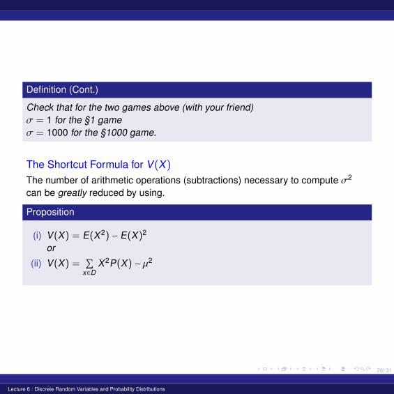
Definition (Cont.)

Check that for the two games above (with your friend)σ = 1 for the §1 gameσ = 1000 for the §1000 game.

The Shortcut Formula for V(X)

The number of arithmetic operations (subtractions) necessary to compute σ2

can be greatly reduced by using.

Proposition

(i) V(X) = E(X2) − E(X)2

or

(ii) V(X) =∑

x∈DX2P(X) − µ2


29/ 31

Proposition (Cont.)

In the formula (*) you need ](D) subtractions (for each x ∈ D you here tosubtract µ then square ...). For the shortcut formula you need only one. Alwaysuse the shortcut formula.

Remark

Logically, version (i) of the shortcut formula is not correct because we haven’t yetdefined the random variable X2.We will do this soon - “change of random variable”.


30/ 31

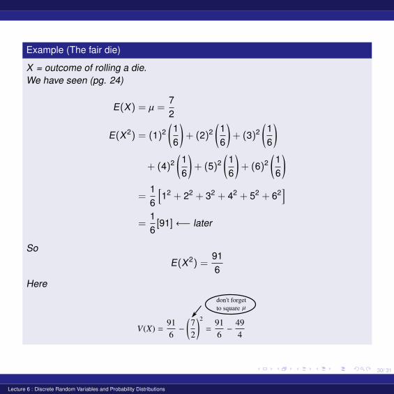
Example (The fair die)

X = outcome of rolling a die.We have seen (pg. 24)

E(X) = µ =72

E(X2) = (1)2(16

)+ (2)2

(16

)+ (3)2

(16

)+ (4)2

(16

)+ (5)2

(16

)+ (6)2

(16

)=

16

[12 + 22 + 32 + 42 + 52 + 62

]=

16[91]←− later

SoE(X2) =

916

Here

don't forget

to square


31/ 31

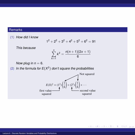
Remarks

(1) How did I know12 + 22 + 32 + 42 + 52 + 62 = 91

This becausen∑

k=1

k 2 =n(n + 1)(2x + 1)

6

Now plug in n = 6.

(2) In the formula for E(X2) don’t square the probabilities

Not squared

first value

squaredsecond value

squared


lecture 6 : discrete random variables and probability...

Documents