DRAFT

Lectures on effective field theory

David B. Kaplan

February 26, 2016

Abstract

Lectures delivered at the ICTP-SAFIR, Sao Paulo, Brasil, February 22-26, 2016.

Contents

1 Effective Quantum Mechanics 31.1 What is an effective field theory? . . . . . . . . . . . . . . . . . . . . . . . . 31.2 Scattering in 1D . . . . . . . . . . . . . . . . . . . . . . . . . . . . . . . . . 4

1.2.1 Square well scattering in 1D . . . . . . . . . . . . . . . . . . . . . . . 41.2.2 Relevant δ-function scattering in 1D . . . . . . . . . . . . . . . . . . 5

1.3 Scattering in 3D . . . . . . . . . . . . . . . . . . . . . . . . . . . . . . . . . 51.3.1 Square well scattering in 3D . . . . . . . . . . . . . . . . . . . . . . . 71.3.2 Irrelevant δ-function scattering in 3D . . . . . . . . . . . . . . . . . . 8

1.4 Scattering in 2D . . . . . . . . . . . . . . . . . . . . . . . . . . . . . . . . . 111.4.1 Square well scattering in 2D . . . . . . . . . . . . . . . . . . . . . . . 111.4.2 Marginal δ-function scattering in 2D & asymptotic freedom . . . . . 12

1.5 Lessons learned . . . . . . . . . . . . . . . . . . . . . . . . . . . . . . . . . . 151.6 Problems for lecture I . . . . . . . . . . . . . . . . . . . . . . . . . . . . . . 16

2 EFT at tree level 172.1 Scaling in a relativistic EFT . . . . . . . . . . . . . . . . . . . . . . . . . . 17

2.1.1 Dimensional analysis: Fermi’s theory of the weak interactions . . . . 192.1.2 Dimensional analysis: the blue sky . . . . . . . . . . . . . . . . . . . 21

2.2 Accidental symmetry and BSM physics . . . . . . . . . . . . . . . . . . . . 232.2.1 BSM physics: neutrino masses . . . . . . . . . . . . . . . . . . . . . 252.2.2 BSM physics: proton decay . . . . . . . . . . . . . . . . . . . . . . . 26

2.3 BSM physics: “partial compositeness” . . . . . . . . . . . . . . . . . . . . . 272.4 Problems for lecture II . . . . . . . . . . . . . . . . . . . . . . . . . . . . . . 29

1

DRAFT

3 EFT and radiative corrections 303.1 Matching . . . . . . . . . . . . . . . . . . . . . . . . . . . . . . . . . . . . . 303.2 Relevant operators and naturalness . . . . . . . . . . . . . . . . . . . . . . . 343.3 Aside – a parable from TASI 1997 . . . . . . . . . . . . . . . . . . . . . . . 353.4 Landau liquid versus BCS instability . . . . . . . . . . . . . . . . . . . . . . 363.5 Problems for lecture III . . . . . . . . . . . . . . . . . . . . . . . . . . . . . 40

4 Chiral perturbation theory 414.1 Chiral symmetry in QCD . . . . . . . . . . . . . . . . . . . . . . . . . . . . 414.2 Quantum numbers of the meson octet . . . . . . . . . . . . . . . . . . . . . 434.3 The chiral Lagrangian . . . . . . . . . . . . . . . . . . . . . . . . . . . . . . 44

4.3.1 The leading term and the meson decay constant . . . . . . . . . . . 444.3.2 Explicit symmetry breaking . . . . . . . . . . . . . . . . . . . . . . . 45

4.4 Loops and power counting . . . . . . . . . . . . . . . . . . . . . . . . . . . . 484.4.1 Subleading order: the O(p4) chiral Lagrangian . . . . . . . . . . . . 494.4.2 Calculating loop effects . . . . . . . . . . . . . . . . . . . . . . . . . 504.4.3 Renormalization of 〈0|qq|0〉 . . . . . . . . . . . . . . . . . . . . . . . 514.4.4 Using the Chiral Lagrangian . . . . . . . . . . . . . . . . . . . . . . 53

4.5 Problems for lecture IV . . . . . . . . . . . . . . . . . . . . . . . . . . . . . 54

5 Effective field theory with baryons 555.1 Transformation properties and meson-baryon couplings . . . . . . . . . . . . 555.2 An EFT for nucleon-nucleon scattering . . . . . . . . . . . . . . . . . . . . . 575.3 The pion-less EFT for nucleon-nucleon interactions . . . . . . . . . . . . . . 58

5.3.1 The case of a “natural” scattering length: 1/|a| ' Λ . . . . . . . . . 605.3.2 The realistic case of an “unnatural” scattering length . . . . . . . . 625.3.3 Beyond the effective range expansion . . . . . . . . . . . . . . . . . . 66

5.4 Including pions . . . . . . . . . . . . . . . . . . . . . . . . . . . . . . . . . . 69

6 Chiral lagrangians for BSM physics 706.1 Technicolor . . . . . . . . . . . . . . . . . . . . . . . . . . . . . . . . . . . . 706.2 Composite Higgs . . . . . . . . . . . . . . . . . . . . . . . . . . . . . . . . . 71

6.2.1 The axion . . . . . . . . . . . . . . . . . . . . . . . . . . . . . . . . . 736.2.2 Axion cosmology and the anthropic axion . . . . . . . . . . . . . . . 766.2.3 The Relaxion . . . . . . . . . . . . . . . . . . . . . . . . . . . . . . . 77

2

DRAFT

1 Effective Quantum Mechanics

1.1 What is an effective field theory?

The uncertainty principle tells us that to probe the physics of short distances we need highmomentum. On the one hand this is annoying, since creating high relative momentumin a lab costs a lot of money! On the other hand, it means that we can have predictivetheories of particle physics at low energy without having to know everything about physicsat short distances. For example, we can discuss precision radiative corrections in the weakinteractions without having a grand unified theory or a quantum theory of gravity. Theprice we pay is that we have a number of parameters in the theory (such as the Higgsand fermion masses and the gauge couplings) which we cannot predict but must simplymeasure. But this is a lot simpler to deal with than a mess like turbulent fluid flow wherethe physics at many different distance scales are all entrained together.

The basic idea behind effective field theory (EFT) is the observation that the non-analytic parts of scattering amplitudes are due to intermediate process where physicalparticles can exist on shell (that is, kinematics are such that internal propagators 1/(p2 −m2 + iε) in Feynman diagrams can diverge with p2 = m2 so that one is sensitive to the iεand sees cuts in the amplitude due to logarithms, square roots, etc). Therefore if one canconstruct a quantum field theory that correctly accounts for these light particles, then allthe contributions to the amplitude from virtual heavy particles that cannot be physicallycreated at these energies can be Taylor expanded p2/M2, where M is the energy of theheavy particle. (By “heavy” I really mean a particle whose energy is too high to create;this might be a heavy particle at rest, but it equally well applies to a pair of light particleswith high relative momentum.) However, the power of of this observation is not that one canTaylor expand parts of the scattering amplitude, but that the Taylor expanded amplitudecan be computed directly from a quantum field theory (the EFT) which contains only lightparticles, with local interactions between them that encode the small effects arising fromvirtual heavy particle exchange. Thus the standard model does not contain X gauge bosonsfrom the GUT scale, for example, but can be easily modified to account for the very smalleffects such particles could have, such as causing the proton to decay, for example.

So in fact, all of our quantum field theories are EFTs; only if there is some day aTheory Of Everything (don’t hold your breath) will we be able to get beyond them. Sohow is a set of lectures on EFT different than a quick course on quantum field theory?Traditionally a quantum field theory course is taught from the point of view that heldsway from when it was originated in the late 1920s through the development of nonabeliangauge theories in the early 1970s: one starts with a φ4 theory at tree level, and thencomputes loops and encounters renormalization; one then introduces Dirac fermions andYukawa interactions, moves on to QED, and then nonabelian gauge theories. All of thesetheories have operators of dimension four or less, and it is taught that this is necessary forrenormalizability. Discussion of the Fermi theory of weak interactions, with its dimension sixfour-fermion operator, is relegated to particle physics class. In contrast, EFT incorporatesthe ideas of Wilson and others that were developed in the early 1970s and completely turnedon its head how we think about UV (high energy) physics and renormalization, and how we

3

DRAFT

interpret the results of calculations. While the φ4 interaction used to be considered one onlyfew well-defined (renormalizable) field theories and the Fermi theory of weak interactionswas viewed as useful but nonrenormalizable and sick, now the scalar theory is consideredsick, while the Fermi theory is a simple prototype of all successful quantum field theories.The new view brings with it its own set of problems, such as an obsession with the fact theour universe appears to be fine-tuned. Is the modern view the last word? Probably not,and I will mention unresolved mysteries at the end of my lectures.

There are three basic uses for effective field theory I will touch on in these lectures:

• Top-down: you know the theory to high energies, but either you do not need all ofits complications to arrive at the desired description of low energy physics, or else thefull theory is nonperturbative and you cannot compute in it, so you construct an EFTfor the light degrees of freedom, constraining their interactions from your knowledgeof the symmetries of the more complete theory;

• Bottom-up: you explore small effects from high dimension operators in your low energyEFT to gain cause about what might be going on at shorter distances than you candirectly probe;

• Philosophizing: you marvel at how “fine-tuned” our world appears to be, and ponder-ing whether the way our world appears is due to some missing physics, or because welive in a special corner of the universe (the anthropic principle), or whether we live ata dynamical fixed point resulting from cosmic evolution. Such investigations are atthe same time both fascinating — and possibly an incredible waste of time!

To begin with I will not discuss effective field theories, however, but effective quantummechanics. The essential issues of approximating short range interactions with point-likeinteractions have nothing to do with relativity or many-body physics, and can be seen inentirety in non-relativistic quantum mechanics. I thought I would try this introductionbecause I feel that the way quantum mechanics and quantum field theory are traditionallytaught it looks like they share nothing in common except for mysterious ladder operators,which is of course not true. What this will consist of is a discussion of scattering fromdelta-function potentials in different dimensions.

1.2 Scattering in 1D

1.2.1 Square well scattering in 1D

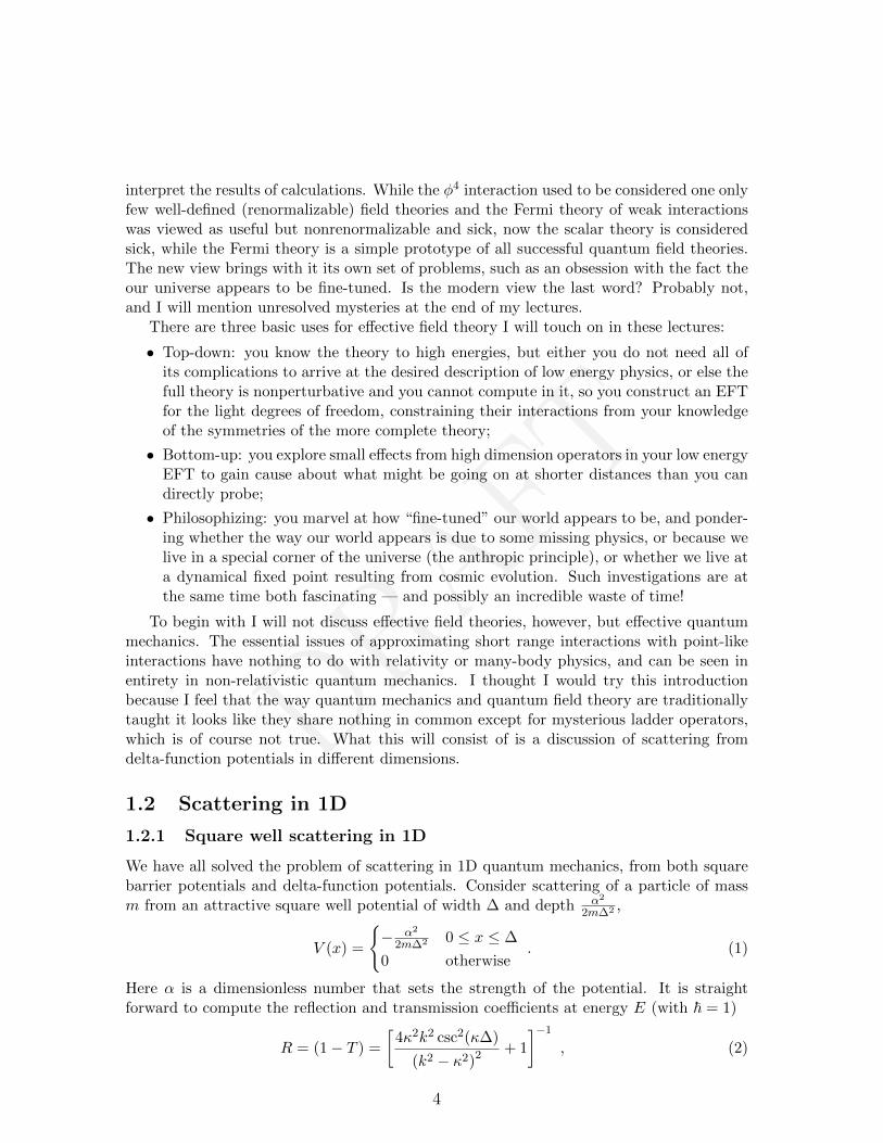
We have all solved the problem of scattering in 1D quantum mechanics, from both squarebarrier potentials and delta-function potentials. Consider scattering of a particle of massm from an attractive square well potential of width ∆ and depth α2

2m∆2 ,

V (x) =

− α2

2m∆2 0 ≤ x ≤ ∆

0 otherwise. (1)

Here α is a dimensionless number that sets the strength of the potential. It is straightforward to compute the reflection and transmission coefficients at energy E (with ~ = 1)

R = (1− T ) =

[4κ2k2 csc2(κ∆)

(k2 − κ2)2 + 1

]−1

, (2)

4

DRAFT

where

k =√

2mE , κ =

√k2 +

α2

∆2. (3)

For low k we can expand the reflection coefficient and find

R = 1− 4

α2 sin2 α∆2k2 +O(∆4k4) (4)

Note that R → 1 as k → 0, meaning that the potential has a huge effect at low enoughenergy, no matter how weak...we can say the interaction is very relevant at low energy.

1.2.2 Relevant δ-function scattering in 1D

Now consider scattering off a δ-function potential in 1D,

V (x) = − g

2m∆δ(x) , (5)

where the length scale ∆ was included in order to make the coupling g dimensionless. Againone can compute the reflection coefficient and find

R = (1− T ) =

[1 +

4k2∆2

g2

]−1

= 1− 4k2∆2

g2+O(k4) . (6)

By comparing the above expression to eq. (4) we see that at low momentum the δ functiongives the same reflection coefficient to up to O(k4) as the square well, provided we set

g = α sinα . (7)

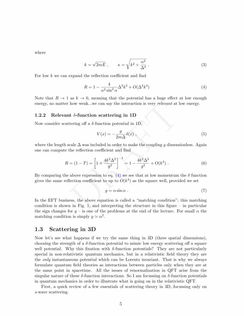
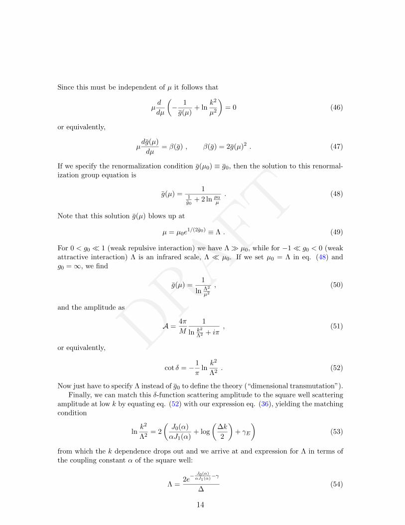
In the EFT business, the above equation is called a “matching condition”; this matchingcondition is shown in Fig. 1, and interpreting the structure in this figure – in particularthe sign changes for g – is one of the problems at the end of the lecture. For small α thematching condition is simply g ' α2.

1.3 Scattering in 3D

Now let’s see what happens if we try the same thing in 3D (three spatial dimensions),choosing the strength of a δ-function potential to mimic low energy scattering off a squarewell potential. Why this fixation with δ-function potentials? They are not particularlyspecial in non-relativistic quantum mechanics, but in a relativistic field theory they arethe only instantaneous potential which can be Lorentz invariant. That is why we alwaysformulate quantum field theories as interactions between particles only when they are atthe same point in spacetime. All the issues of renormalization in QFT arise from thesingular nature of these δ-function interactions. So I am focussing on δ-function potentialsin quantum mechanics in order to illustrate what is going on in the relativistic QFT.

First, a quick review of a few essentials of scattering theory in 3D, focussing only ons-wave scattering.

5

DRAFT

2 4 6 8 10α

-6

-4

-2

2

4

6

8

g

Figure 1: The matching condition in 1D: the appropriate value of g in the effective theory for agiven α in the full theory.

A scattering solution for a particle of mass m in a finite range potential must have theasymptotic form for large |r|

ψr→∞−−−→ eikz +

f(θ)

reikr . (8)

representing an incoming plane wave in the z direction, and an outgoing scattered sphericalwave. The quantity f is the scattering amplitude, depending both on scattering angle θand incoming momentum k, and |f |2 encodes the probability for scattering; in particular,the differential cross section is simply

dσ

dθ= |f(θ)|2 . (9)

For scattering off a spherically symmetric potential, both f(θ) and eikz = eikr cos θ can beexpanded in Legendre polynomials (“partial wave expansion”); I will only be interestedin s-wave scattering (angle independent) and therefore will replace f(θ) simply by f —independent of angle, but still a function of k. For the plane wave we can average over θwhen only considering s-wave scattering, replacing

eikz = eikr cos θ −−−−→s−wave

1

2

∫ π

0dθ sin θ eikr cos θ = j0(kr) . (10)

Here j0(z) is a regular spherical Bessel function; we will also meet its irregular partnern0(z), where where

j0(z) =sin z

z, n0(z) = −cos z

z. (11)

These functions are the s-wave solutions to the free 3D Schrodinger equation z = kr.So we are interested in a solution to the Schrodinger equation with asymptotic behavior

ψr→∞−−−−→s−wave

j0(kr) +f

reikr = j0(kr) + kf (ij0(kr)− n0(kr)) (s-wave) (12)

6

DRAFT

Since outside the the range of the potential ψ is an exact s-wave solution to the freeSchrodinger equation, and the most general solutions to the free radial Schrodinger equationare the spherical Bessel functions j0(kr), n0(kr), the asymptotic form for ψ can also bewritten as

ψr→∞−−−→ A (cos δ j0(kr)− sin δ n0(kr)) . (13)

where A and δ are real constants. The angle δ is called the phase shift, and if there was nopotential, boundary conditions at r = 0 would require δ = 0...so nonzero δ is indicative ofscattering. Relating these two expressions eq. (12) and eq. (13) we find

f =1

k cot δ − ik. (14)

So solving for the phase shift δ is equivalent to solving for the scattering amplitude f , usingthe formula above.

The quantity k cot δ is interesting, since one can show that for a finite range potentialit must be analytic in the energy, and so has a Taylor expansion in k involving only evenpowers of k , called “the effective range expansion”:

k cot δ = −1

a+

1

2r0k

2 +O(k4) . (15)

The parameters have names: a is the scattering length and r0 is the effective range; theseterms dominate low energy (low k) scattering. Proving the existence of the effective rangeexpansion is somewhat involved and I refer you to a quantum mechanics text; there is alow-brow proof due to Bethe and a high-brow one due to Schwinger.

And the last part of this lightning review of scattering: if we have two particles of massM scattering off each other it is often convenient to use Feynman diagrams to describe thescattering amplitude; I denote the Feynman amplitude – the sum of all diagrams – as iA.The relation between A and f is

A =4π

Mf , (16)

where f is the scattering amplitude for a single particle of reduced mass m = M/2 in theinter-particle potential. This proportionality is another result that can be priced togetherfrom quantum mechanics books, which I won’t derive.

1.3.1 Square well scattering in 3D

We consider s-wave scattering off an attractive well in 3D,

V =

− α2

m∆2 r < ∆

0 r > ∆ .(17)

We have for the wave functions for the two regions r < ∆, r > ∆ are expressed in terms ofspherical Bessel functions as

ψ<(r) = j0(κr) , ψ>(r) = A [cos δ j0(kr)− sin δ n0(kr)] (18)

7

DRAFT

2 4 6 8 10α

-2

-1

1

2

3

a/Δ

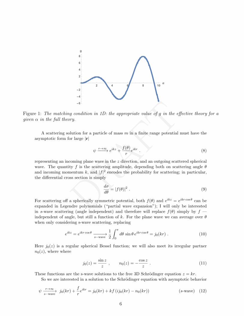
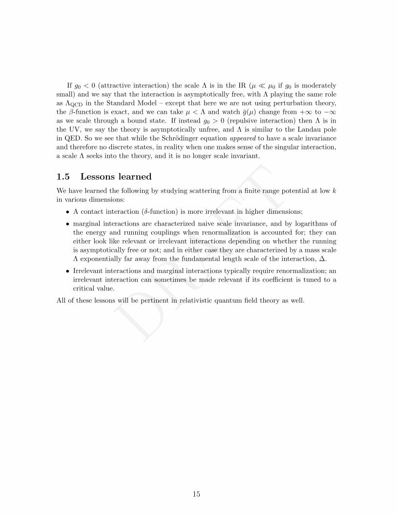
Figure 2: a/∆ vs. the 3D potential well depth parameter α, from eq. (21).

where κ =√k2 + α2/∆2 as in eq. (3) and δ is the s-wave phase shift. Equating ψ and ψ′

at the edge of the potential at r = ∆ allows us to solve for δ in terms of k, α,∆, with theresult

k cot δ =k(k sinκ∆ + κ cot k∆ cosκ∆)

k cot k∆ sinκ∆− κ cosκ∆. (19)

With a little help from Mathematica we can expand this in powers of k2 and find

k cot δ =1

∆

(tanα

α− 1

)−1

+O(k2) (20)

where on comparing with eq. (15) we can read off the scattering length from the k2

expansion,

a = −∆

(tanα

α− 1

), (21)

a relation shown in Fig. 2. The singularities one finds for the scattering length as thestrength of the potential α increases correspond to the critical values αc = (2n + 1)π/2,n = 0, 1, 2 . . . where a new bound state appears.

1.3.2 Irrelevant δ-function scattering in 3D

Now we look at reproducing the above scattering length from scattering in 3D off a deltafunction potential. At first look this seems hopeless: note that the result for a square wellof width ∆ and coupling α = O(1) gives a scattering length that is a = O(∆); this is to beexpected since a is a length, and ∆ is the natural length scale in the problem. Thereforeif you extrapolate to a potential of zero width (a δ function) you would conclude that thescattering length would go to zero, and the scattering amplitude would vanish for low k.This is an example of an irrelevant interaction.

On second look the situation is even worse: since −δ3(r) scales as −1/r3 while the kinetic−∇2 term in the Schrodinger equation only scales as 1/r2 you can see that the systemdoes not have a finite energy ground state. For example if you performed a variational

8

DRAFT

calculation, you could lower the energy without bound by scaling the wave function tosmaller and smaller extent. Therefore the definition of a δ-function has to be modified in3D – this is the essence of renormalization.

These two features go hand in hand: typically singular interactions are “irrelevant” andat the same time require renormalization. We can sometimes turn an irrelevant interactioninto a relevant one by fixing a certain renormalization condition which forces a fine tuningof the coupling to a critical value, and that is the case here. For example, consider definingthe δ-function as the ρ→ 0 limit of a square well of width ρ and depth V0 = α2(ρ)/(mρ2),while adjusting the coupling strength α(ρ) to keep the scattering length fixed to the desiredvalue of a given in eq. (21). We find

a = ρ

(1− tan α(ρ)

α(ρ)

)(22)

as ρ→ 0. There are an infinite number of solutions, corresponding to α ' αc = (2n+1)π/2,n = 0, 1, 2 . . . , and the n = 0 possibility is

α(ρ)ρ→0−−−→ π

2+

2ρ

πa+O(ρ2) . (23)

in other words, we have to tune this vanishingly thin square well to have a single boundstate right near threshold (α ' π/2). However, note that while naively you might think apotential −gδ3(r) would be approximated by a square well of depth V0 ∝ 1/ρ3 as ρ → 0,but we see that instead we get V0 ∝ 1/ρ2. This is sort of like using a potential −rδ3(r)instead of −δ3(r).

We have struck a delicate balance: A naive δ function potential is too strong and singularto have a ground state; a typical square well of depth α2/mρ2 becomes irrelevant for fixedα in the ρ→ 0 limit; but a strongly coupled potential of form V ' −(π/2)2/mρ2 can leadto a relevant interaction so long as we tune α its critical value αc = π/2 in precisely theright way as we take ρ→ 0.

This may all seem more familiar to you if I to use field theory methods and renor-malization. Consider two colliding particles of mass M in three spatial dimensions witha δ-function interaction; this is identical to the problem of potential scattering when weidentify m with the reduced mass of the two particle system,

m =M

2. (24)

We introduce the field ψ for the scattering particles (assuming they are spinless bosons)and the Lagrange density

L = ψ†(i∂t +

∇2

2M

)ψ − C0

4

(ψ†ψ

)2. (25)

Here C0 > 0 implies a repulsive interaction. As in a relativistic field theory, ψ annihilatesparticles and ψ† creates them; unlike in a relativistic field theory, however, there are noanti-particles.

9

DRAFT

+ + +…

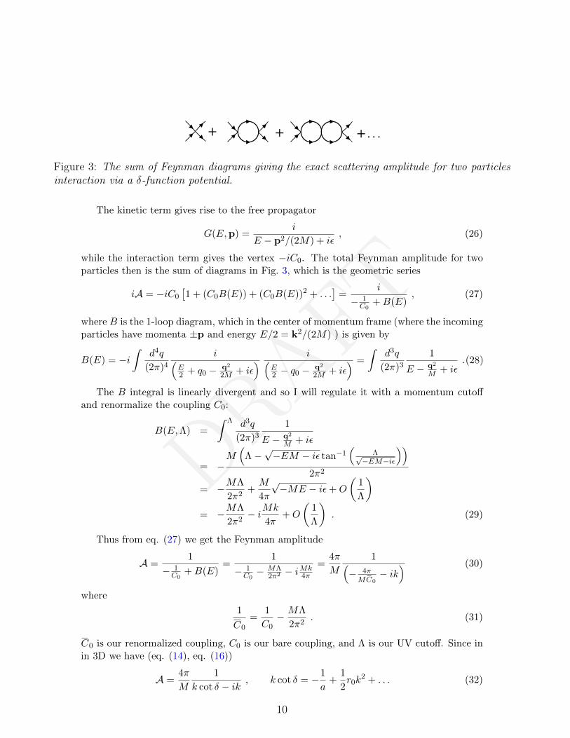
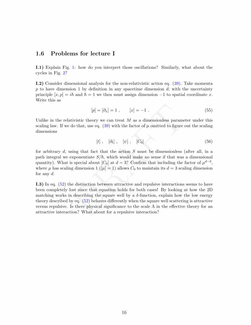
Figure 3: The sum of Feynman diagrams giving the exact scattering amplitude for two particlesinteraction via a δ-function potential.

The kinetic term gives rise to the free propagator

G(E,p) =i

E − p2/(2M) + iε, (26)

while the interaction term gives the vertex −iC0. The total Feynman amplitude for twoparticles then is the sum of diagrams in Fig. 3, which is the geometric series

iA = −iC0

[1 + (C0B(E)) + (C0B(E))2 + . . .

]=

i

− 1C0

+B(E), (27)

where B is the 1-loop diagram, which in the center of momentum frame (where the incomingparticles have momenta ±p and energy E/2 = k2/(2M) ) is given by

B(E) = −i∫

d4q

(2π)4

i(E2 + q0 − q2

2M + iε) i(

E2 − q0 − q2

2M + iε) =

∫d3q

(2π)3

1

E − q2

M + iε.(28)

The B integral is linearly divergent and so I will regulate it with a momentum cutoffand renormalize the coupling C0:

B(E,Λ) =

∫ Λ d3q

(2π)3

1

E − q2

M + iε

= −M(

Λ−√−EM − iε tan−1

(Λ√

−EM−iε

))2π2

= −MΛ

2π2+M

4π

√−ME − iε+O

(1

Λ

)= −MΛ

2π2− iMk

4π+O

(1

Λ

). (29)

Thus from eq. (27) we get the Feynman amplitude

A =1

− 1C0

+B(E)=

1

− 1C0− MΛ

2π2 − iMk4π

=4π

M

1(− 4πMC0

− ik) (30)

where

1

C0

=1

C0− MΛ

2π2. (31)

C0 is our renormalized coupling, C0 is our bare coupling, and Λ is our UV cutoff. Since inin 3D we have (eq. (14), eq. (16))

A =4π

M

1

k cot δ − ik, k cot δ = −1

a+

1

2r0k

2 + . . . (32)

10

DRAFT

we see that this theory relates C0 to the scattering length as

C0 =4πa

M. (33)

Therefore we can reproduce square well scattering length eq. (21) by taking

C0 = −4π∆

M

(tanα

α− 1

). (34)

With our simple EFT we can reproduce the scattering length of the square well problem,but not the next term in the low k expansion, the effective range. There is a one-to-onecorrespondence between the number of terms we can fit in the effective range expansionand the number of operators we include in the EFT; to account for the effective range wewould have to include a new contact interaction involving two derivatives and match itscoefficient.

What have we accomplished? We have shown that one can reproduce low energy scatter-ing from a finite range potential in 3D with a δ-function interaction, with errors of O(k2∆2)with the caveat that renormalization is necessary if we want to make sense of the theory.

However there is second important and subtle lesson: We can view eq. (31) plus eq. (33)to imply a fine tuning of the inverse bare coupling 1/C0 coupling as Λ→∞: MΛC0/(2π

2)must be tuned to 1 + O(1/aΛ) as Λ → ∞. This is the same lesson we learned looking atsquare wells: if C0 didn’t vanish at least linearly with the cutoff, the interaction would betoo strong to makes sense; while if ΛC0 went to zero or a small constant, the interactionwould be irrelevant. Only if ΛC0 is fine-tuned to a critical value can we obtain nontrivialscattering at low k.

1.4 Scattering in 2D

1.4.1 Square well scattering in 2D

Finally, let’s look at the intermediary case of scattering in two spatial dimensions, wherewe take the same potential as in eq. (17). This is not just a tour of special functions —something interesting happens! The analogue of eq. (35) for the two dimensional squarewell problem is

ψ<(r) = J0(κr) , ψ>(r) = A [cos δ J0(kr)− sin δ Y0(kr)] (35)

where κ is given in eq. (3) and J , Y are the regular and irregular Bessel functions. Equatingψ and ψ′ at the boundary r = ∆ gives1

cot δ =kJ0(∆κ)Y1(∆k)− κJ1(∆κ)Y0(∆k)

kJ0(∆κ)J1(∆k)− κJ1(∆κ)J0(k∆)

=2(J0(α)αJ1(α) + log

(∆k2

)+ γE

)π

+O(k2)

(36)

1In the following expressions γE = 0.577 . . . is the Euler constant.

11

DRAFT

This result looks very odd because of the logarithm that depends on k! The interestingfeature of this expression is not that cot δ(k) → −∞ for k → 0: that just means thatthe phase shift vanishes at low k. What is curious is that for our attractive potential, thefunction J0(α)/(αJ1(α)) is strictly positive, and therefore cot δ changes sign at a specialvalue for k,

k = Λ ' 2e− J0(α)αJ1(α)

−γE

∆, (37)

where the scale Λ is exponentially lower than our fundamental scale ∆ for weak coupling,since then J0(α)/αJ1(α) ∼ 2/α2 1. This is evidence in the scattering amplitude for abound state of size ∼ 1/Λ...exponentially larger than the size of the potential!

On the other hand, if the interaction is repulsive, the J0(α)/αJ1(α) factor is replacedby −I0(α)/αI1(α) < 0, In being one of the other Bessel functions, and the numerator ineq. (36) is always negative, and there is no bound state.

1.4.2 Marginal δ-function scattering in 2D & asymptotic freedom

If we now look at the Schrodinger equation with a δ-function to mock up the effects of thesquare well for low k we find something funny: the equation is scale invariant. What thatmeans is that the existence of any solution ψ(r) to the equation[

− 1

2m∇2 +

g

mδ2(r)

]ψ(r) = Eψ(r) (38)

implies a continuous family of solutions ψλ(r) = ψ(λr) – the same functional form exceptscaled smaller by a factor of λ – with energy Eλ = λ2E. Thus it seems that all possibleenergy eigenvalues with the same sign as E exist and there are no discrete eigenstates...whichis OK if only positive energy scattering solutions exist, the case for a repulsive interaction— but not OK if there are bound states: it appears that if there is any one negative energystate, then there is an unbounded continuum of negative energy states and no ground state.The problem is that ∇2 and δ2(r) have the same dimension, 1/length2, and so there is noinherent scale to the left side of the equation. Since the scaling property of δD(r) changeswith dimension D, while the scaling property of ∇2 does not, D = 2 is special.

Since the δ-function interaction seems to be scale invariant, we say that it is neitherrelevant (dominating IR physics, as in 1D) nor irrelevant (unimportant to IR physics, as in3D) but apparently of equal important at all scales, which we call marginal. However, weknow that (i) the δ function description appears to be sick, and (ii) from our exact analysisof the square well that the IR description of the full theory is not really scale invariant,due to the logarithm. Therefore it is a reasonable guess that our analysis of the δ-functionis incorrect due to its singularity, and that we are going to have to be more careful, andrenormalize.

We can repeat the Feynman diagram approach we used in 3D, only now in 2D. Now theloop integral in eq. (29) is required in d = 3 spacetime dimensions instead of d = 4. It is stilldivergent, but now only log divergent, not linearly divergent. It still needs regularization,but this time instead of using a momentum cutoff I will use dimensional regularization, to

12

DRAFT

make it look even more like conventional QFT calculations. Therefore we keep the numberof spacetime dimensions d arbitrary in computing the integral, and subsequently expandabout d = 3 (for scattering in D = 2 spatial dimensions)2. We take for our action

S =

∫dt

∫dd−1x

[ψ†(i∂t +

∇2

2M

)ψ − µd−3C0

4

(ψ†ψ

)2]. (39)

where the renormalization scale µ was introduced to keep C0 dimensionless (see problem).Then the Feynman rules are the same as in the previous case, except for the factor of µd−3

at the vertices, and we find

B(E) = µ3−d∫

dd−1q

(2π)d−1

1

E − q2

M + iε

= −M (−ME − iε)d−32 Γ

(3− d

2

)µ3−d

(4π)(d−1)/2

d→3−−−→ M

2π

1

(d− 3)+M

4π

(γE − ln 4π + ln

k2

µ2− iπ

)+O(d− 3) (40)

where k =√ME is the magnitude of the momentum of each incoming particle in the center

of momentum frame, and the scattering amplitude is therefore

A =1

− 1C0

+B(E)=

[− 1

C0+M

2π

1

(d− 3)+M

4π

(γE − ln 4π + ln

k2

µ2− iπ

)]−1

(41)

At this point it is convenient to define the dimensionless coupling constant g:

C0 ≡ g4π

M. (42)

Given the definition of our Lagrangian, g > 0 corresponds to a repulsive potential, andg < 0 is attractive. so that the amplitude is

A =4π

M

[−1

g− 2

(d− 3)+ γE − ln 4π + ln

k2

µ2− iπ

]−1

(43)

To make sense of this at d = 3 we have to renormalize g with the definition:

1

g=

1

g(µ)+

2

(d− 3)+ γE − ln 4π , (44)

where g(µ) is the renormalized running coupling constant, and so the amplitude is given by

A =4π

M

[− 1

g(µ)+ ln

k2

µ2− iπ

]−1

(45)

2If you are curious why I did not use dimensional regularization for the D = 3 case: dim reg ignores powerdivergences, and so when computing graphs with power law divergences using dim reg you do not explicitly noticethat you are fine-tuning the theory. This happens in the standard model with the quadratic divergence of theHiggs mass2...every few years someone publishes a preprint saying there is no fine-tuning problem since one cancompute diagrams using dim reg, where there is no quadratic divergence, which is silly. I used a momentumcutoff in the previous section so we could see the fine-tuning of C0.

13

DRAFT

Since this must be independent of µ it follows that

µd

dµ

(− 1

g(µ)+ ln

k2

µ2

)= 0 (46)

or equivalently,

µdg(µ)

dµ= β(g) , β(g) = 2g(µ)2 . (47)

If we specify the renormalization condition g(µ0) ≡ g0, then the solution to this renormal-ization group equation is

g(µ) =1

1g0

+ 2 ln µ0µ

. (48)

Note that this solution g(µ) blows up at

µ = µ0e1/(2g0) ≡ Λ . (49)

For 0 < g0 1 (weak repulsive interaction) we have Λ µ0, while for −1 g0 < 0 (weakattractive interaction) Λ is an infrared scale, Λ µ0. If we set µ0 = Λ in eq. (48) andg0 =∞, we find

g(µ) =1

ln Λ2

µ2

, (50)

and the amplitude as

A =4π

M

1

ln k2

Λ2 + iπ, (51)

or equivalently,

cot δ = − 1

πlnk2

Λ2. (52)

Now just have to specify Λ instead of g0 to define the theory (“dimensional transmutation”).Finally, we can match this δ-function scattering amplitude to the square well scattering

amplitude at low k by equating eq. (52) with our expression eq. (36), yielding the matchingcondition

lnk2

Λ2= 2

(J0(α)

αJ1(α)+ log

(∆k

2

)+ γE

)(53)

from which the k dependence drops out and we arrive at and expression for Λ in terms ofthe coupling constant α of the square well:

Λ =2e− J0(α)αJ1(α)

−γ

∆(54)

14

DRAFT

If g0 < 0 (attractive interaction) the scale Λ is in the IR (µ µ0 if g0 is moderatelysmall) and we say that the interaction is asymptotically free, with Λ playing the same roleas ΛQCD in the Standard Model – except that here we are not using perturbation theory,the β-function is exact, and we can take µ < Λ and watch g(µ) change from +∞ to −∞as we scale through a bound state. If instead g0 > 0 (repulsive interaction) then Λ is inthe UV, we say the theory is asymptotically unfree, and Λ is similar to the Landau polein QED. So we see that while the Schrodinger equation appeared to have a scale invarianceand therefore no discrete states, in reality when one makes sense of the singular interaction,a scale Λ seeks into the theory, and it is no longer scale invariant.

1.5 Lessons learned

We have learned the following by studying scattering from a finite range potential at low kin various dimensions:

• A contact interaction (δ-function) is more irrelevant in higher dimensions;

• marginal interactions are characterized naive scale invariance, and by logarithms ofthe energy and running couplings when renormalization is accounted for; they caneither look like relevant or irrelevant interactions depending on whether the runningis asymptotically free or not; and in either case they are characterized by a mass scaleΛ exponentially far away from the fundamental length scale of the interaction, ∆.

• Irrelevant interactions and marginal interactions typically require renormalization; anirrelevant interaction can sometimes be made relevant if its coefficient is tuned to acritical value.

All of these lessons will be pertinent in relativistic quantum field theory as well.

15

DRAFT

1.6 Problems for lecture I

I.1) Explain Fig. 1: how do you interpret those oscillations? Similarly, what about thecycles in Fig. 2?

I.2) Consider dimensional analysis for the non-relativistic action eq. (39). Take momentap to have dimension 1 by definition in any spacetime dimension d; with the uncertaintyprinciple [x, p] = i~ and ~ = 1 we then must assign dimension −1 to spatial coordinate x.Write this as

[p] = [∂x] = 1 , [x] = −1 . (55)

Unlike in the relativistic theory we can treat M as a dimensionless parameter under thisscaling law. If we do that, use eq. (39) with the factor of µ omitted to figure out the scalingdimensions

[t] , [∂t] , [ψ] , [C0] (56)

for arbitrary d, using that fact that the action S must be dimensionless (after all, in apath integral we exponentiate S/~, which would make no sense if that was a dimensionalquantity). What is special about [C0] at d = 3? Confirm that including the factor of µd−3,where µ has scaling dimension 1 ([µ] = 1) allows C0 to maintain its d = 3 scaling dimensionfor any d.

I.3) In eq. (52) the distinction between attractive and repulsive interactions seems to havebeen completely lost since that equation holds for both cases! By looking at how the 2Dmatching works in describing the square well by a δ-function, explain how the low energytheory described by eq. (52) behaves differently when the square well scattering is attractiveversus repulsive. Is there physical significance to the scale Λ in the effective theory for anattractive interaction? What about for a repulsive interaction?

16

DRAFT

2 EFT at tree level

To construct a relativistic effective field theory valid up to some scale Λ, we will take for ouraction made out of all light fields (those corresponding to particles with masses or energiesmuch less that Λ) including all possible local operators consistent with the underlyingsymmetries that we think govern the world. All UV physics that we are not includingexplicitly is encoded in the coefficients of these operators, in the same way we saw in theprevious section that a contact interaction (δ-function potential) was able to reproduce thescattering length for scattering off a square well if its coefficient was chosen appropriately(we “matched” it to the UV physics). However, in the previous examples we just triedmatching the scattering lengths; we could have tried to also reproduce O(k2∆2) effects, andso on, but to do so would have required introducing more and more singular contributions tothe potential in the effective theory, such as ∇2δ(r), ∇4δ(r), and so on. Going to all ordersin k2 would require an infinite number of such terms, and the same is true for a relativisticEFT. Such a theory is not “renormalizable” in the historical sense: there is typically nofinite set of coupling constants that can be renormalized with a finite pieces of experimentaldata to render the theory finite. Instead there are an infinite number of counterterms needto make the theory finite, and therefore an infinite number of experimental data needed tofix the finite parts of the counterterms. Such a theory would be unless there existed somesort of expansion that let us deal with only a finite set of operators at each order in thatexpansion.

Wilson provided such an expansion. The first thing to accept is that the EFT has anintrinsic, finite UV cutoff Λ. This scale is typically the mass of the lightest particles omittedfrom the theory. For example, in the Fermi theory of the weak interactions, Λ = MW .With a cutoff in place, all radiative corrections in the theory are finite, even if they areproportional to powers or logarithms of Λ. The useful expansion then is a momentumexpansion, in powers of k/Λ, where k is the external momentum in some physical processof interest, such as a particle decay, two particle scattering, two particle annihilation, etc.This momentum expansion is the key tool that makes EFTs useful. To understand howthis works, we need to develop the concept of operator dimension. In this lecture we willonly consider the EFT at tree level.

2.1 Scaling in a relativistic EFT

As a prototypical example of an EFT, consider the Lagrangian (in four dimensional Eu-clidean spacetime, after a Wick rotation to imaginary time) for relativistic scalar field witha φ→ −φ symmetry:

LE =1

2(∂φ)2 +

1

2m2φ2 +

λ

4!φ4 +

∞∑n=1

(cn

Λ2nφ4+2n +

dnΛ2n

(∂φ)2φ2n + . . .

)(57)

We are setting ~ = c = 1 so that momenta have dimension of mass, and spacetime coordi-nates have dimension of inverse mass. I indicate this as

[p] = 1 , [x] = [t] = −1 , [∂x] = [∂t] = 1 . (58)

17

DRAFT

Since the action is dimensionless, then — in d = 4 spacetime dimensions — from the kineticterm for φ we see that φ has dimension of mass:

[φ] = 1 . (59)

That means that the operator φ6 is dimension 6, and the contribution to the action∫d4xφ6

has dimension 2, and so its coupling constant must have dimension −2, or 1/mass2. Theoperator φ2(∂2φ)2 is dimension 8 and must have a coefficient which is dimension −4, or1/mass4. In eq. (57) I have introduced the cutoff scale Λ explicitly into the Lagrangianin such a way as to make the the couplings λ, cn and dn all dimensionless, with no lossof generality. I will assume here that λ 1, cn 1 and dn 1 so that a perturbativeexpansions in these couplings is reasonable.

You might ask why we do things this way — why not rescale the φ6 operator to havecoefficient 1 instead of the kinetic term, and declare φ to have dimension 2/3? The reasonwhy is because the kinetic term is more important and determines the size of quantumfluctuations for a relativistic excitation. To see this, consider the path integral∫

Dφe−SE , SE =

∫d4xLE . (60)

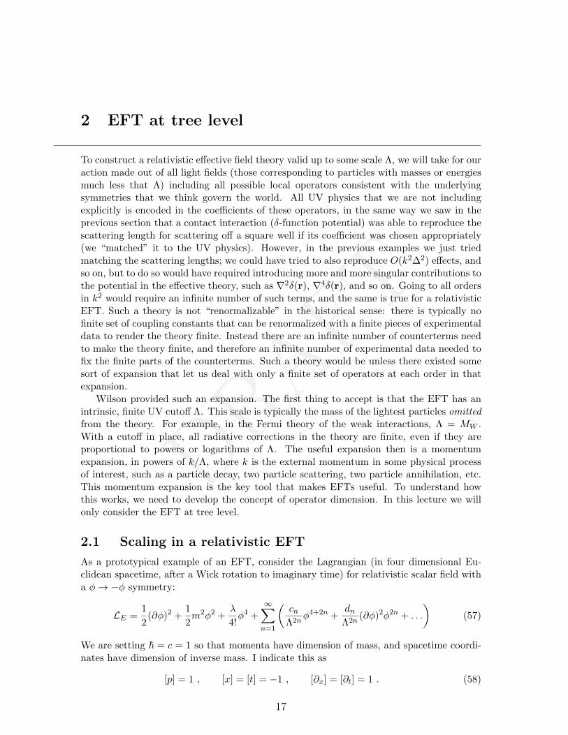
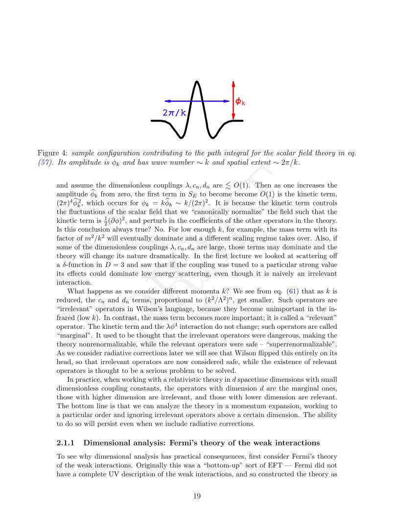
Now consider a particular field configuration contributing to this path integral that lookslike the “wavelet” pictured in Fig. 4, with wavenumber |kµ| ∼ k, localized to a spacetimevolume of size L4, where L ' 2π/k, and with amplitude φk. Derivatives acting on such aconfiguration give powers of k, while spacetime integration gives a factor of L4 ' (4π/k)4.With this configuration, the Euclidean action is given by

SE '(

2π

k

)4[k2φ 2

k

2+

1

2m2φ 2

k +λ

4!φk

4 +∞∑n=1

(cn

Λ2nφk

4+2n +dnk

2

Λ2nφk

2+2n + . . .

)]

= (2π)4

[φ 2k

2+

1

2

m2

k2φ 2k +

λ

4!φ 4k +

∑n

(cn

(k2

Λ2

)nφ 4+2nk + dn

(k2

Λ2

)nφ 2+2nk + . . .

)],

(61)

where in the second line I have rescaled the amplitude by k,

φk ≡ φk/k . (62)

In the above expression, the factor of(

2πk

)4in front is the spacetime volume occupied by

our wavelet and comes from∫d4x, while for every operator I have substituted ∂ → k and

φ → kφk. Now for the path integral, consider ordinary integration over the amplitude φkfor this particular mode: ∫

dφk e−SE . (63)

The integral is dominated by those values of φk for which SE . 1, because otherwiseexp(−SE) is very small. Which are the important terms in SE in this region? First, assumethat the particle is relativistic, m k Λ so that both m2/k2 and k2/Λ2 are very small,

18

DRAFT

2Π!k Φk

Figure 4: sample configuration contributing to the path integral for the scalar field theory in eq.(57). Its amplitude is φk and has wave number ∼ k and spatial extent ∼ 2π/k.

and assume the dimensionless couplings λ, cn, dn are . O(1). Then as one increases theamplitude φk from zero, the first term in SE to become become O(1) is the kinetic term,(2π)4φ 2

k , which occurs for φk = kφk ∼ k/(2π)2. It is because the kinetic term controlsthe fluctuations of the scalar field that we “canonically normalize” the field such that thekinetic term is 1

2(∂φ)2, and perturb in the coefficients of the other operators in the theory.Is this conclusion always true? No. For low enough k, for example, the mass term with itsfactor of m2/k2 will eventually dominate and a different scaling regime takes over. Also, ifsome of the dimensionless couplings λ, cn, dn are large, those terms may dominate and thetheory will change its nature dramatically. In the first lecture we looked at scattering offa δ-function in D = 3 and saw that if the coupling was tuned to a particular strong valueits effects could dominate low energy scattering, even though it is naively an irrelevantinteraction.

What happens as we consider different momenta k? We see from eq. (61) that as k isreduced, the cn and dn terms, proportional to (k2/Λ2)n, get smaller. Such operators are“irrelevant” operators in Wilson’s language, because they become unimportant in the in-frared (low k). In contrast, the mass term becomes more important; it is called a “relevant”operator. The kinetic term and the λφ4 interaction do not change; such operators are called“marginal”. It used to be thought that the irrelevant operators were dangerous, making thetheory nonrenormalizable, while the relevant operators were safe – “superrenormalizable”.As we consider radiative corrections later we will see that Wilson flipped this entirely on itshead, so that irrelevant operators are now considered safe, while the existence of relevantoperators is thought to be a serious problem to be solved.

In practice, when working with a relativistic theory in d spacetime dimensions with smalldimensionless coupling constants, the operators with dimension d are the marginal ones,those with higher dimension are irrelevant, and those with lower dimension are relevant.The bottom line is that we can analyze the theory in a momentum expansion, working toa particular order and ignoring irrelevant operators above a certain dimension. The abilityto do so will persist even when we include radiative corrections.

2.1.1 Dimensional analysis: Fermi’s theory of the weak interactions

To see why dimensional analysis has practical consequences, first consider Fermi’s theoryof the weak interactions. Originally this was a “bottom-up” sort of EFT — Fermi did nothave a complete UV description of the weak interactions, and so constructed the theory as

19

DRAFT

a phenomenological modification of QED to account for neutron decay. Now we have theSM, and so we think of the Fermi theory as a “top-down” EFT: not necessary for doingcalculations since we have the SM, but very practical for processes at energies far belowthe W mass, such as β-decay (Fermi’s original application of his theory) and low energyneutral current scattering due to Z exchange (about which Fermi knew nothing).

The weak interactions refer to processes mediated by the W± or Z0 bosons, whosemasses are approximately 80 GeV and 91 GeV respectively. The couplings of these gaugebosons to quarks and leptons can be written in terms of the electromagnetic current

jµem =2

3uiγ

µui −2

3diγ

µdi − eiγµei (64)

where i = 1, 2, 3 runs over families, and the left-handed SU(2) currents

jµa =∑ψ

ψγµ(

1− γ5

2

)τa2ψ , a = 1, 2, 3 , (65)

where the ψ,ψ fields in the currents are either the lepton doublets(νee

),

(νµµ

),

(νττ

), (66)

or the quark doublets

ψ =

(ud′

),

(cs′

),

(tb′

), (67)

with the “flavor eigenstates” d′, s′ and b′ being related to the mass eigenstates d, s and bby the unitary Cabibbo-Kobayashi-Maskawa (CKM) matrix3:

q′i = Vijqj . (68)

The SM coupling of the heavy gauge bosons to these currents is

LJ =e

sin θw

(W+µ J

µ− +W−µ J

µ+

)+

e

sin θw cos θwZµ(jµ3 − sin2 θwj

µem

)(69)

where

Jµ± =jµ1 ∓ i j

µ2√

2. (70)

Tree level exchange of a W boson then gives the amplitude at low momentum exchange

iA =

(−i e

sin θw

)2

Jµ−Jν+

−igµνq2 −M2

W

= −i e2

sin2 θwM2W

Jµ−Jµ+ +O

(q2

M2W

). (71)

3The elements of the CKM matrix are named after which quarks they couple through the charged current,namely V11 ≡ Vud, V12 ≡ Vus, V21 ≡ Vcd, etc.

20

DRAFT

ψ1

ψ2

ψ3

ψ4

ψ1

ψ2

ψ3

ψ4

W,Z

(a) (b)

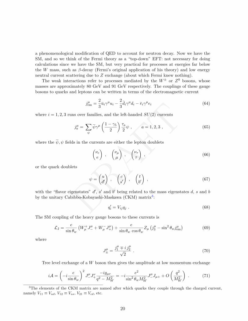
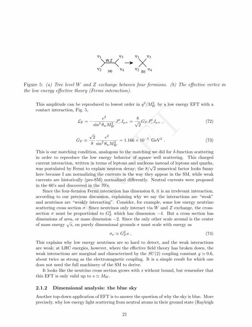
Figure 5: (a) Tree level W and Z exchange between four fermions. (b) The effective vertex inthe low energy effective theory (Fermi interaction).

This amplitude can be reproduced to lowest order in q2/M2W by a low energy EFT with a

contact interaction, Fig. 5,

LF = − e2

sin2 θwM2W

Jµ−Jµ+ =8√2GFJ

µ−Jµ+ , (72)

GF ≡√

2

8

e2

sin2 θwM2W

= 1.166× 10−5 GeV2 . (73)

This is our matching condition, analogous to the matching we did for δ-function scatteringin order to reproduce the low energy behavior of square well scattering. This chargedcurrent interaction, written in terms of leptons and nucleons instead of leptons and quarks,was postulated by Fermi to explain neutron decay; the 8/

√2 numerical factor looks funny

here because I am normalizing the currents in the way they appear in the SM, while weakcurrents are historically (pre-SM) normalized differently. Neutral currents were proposedin the 60’s and discovered in the 70’s.

Since the four-fermion Fermi interaction has dimension 6, it is an irrelevant interaction,according to our previous discussion, explaining why we say the interactions are “weak”and neutrinos are “weakly interacting”. Consider, for example, some low energy neutrinoscattering cross section σ. Since neutrinos only interact via W and Z exchange, the cross-section σ must be proportional to G2

F which has dimension −4. But a cross section hasdimensions of area, or mass dimension −2. Since the only other scale around is the centerof mass energy

√s, on purely dimensional grounds σ must scale with energy as

σν ' G2F s , (74)

This explains why low energy neutrinos are so hard to detect, and the weak interactionsare weak; at LHC energies, however, where the effective field theory has broken down, theweak interactions are marginal and characterized by the SU(2) coupling constant g ' 0.6,about twice as strong as the electromagnetic coupling. It is a simple result for which onedoes not need the full machinery of the SM to derive.

It looks like the neutrino cross section grows with s without bound, but remember thatthis EFT is only valid up to s 'MW .

2.1.2 Dimensional analysis: the blue sky

Another top-down application of EFT is to answer the question of why the sky is blue. Moreprecisely, why low energy light scattering from neutral atoms in their ground state (Rayleigh

21

DRAFT

scattering) is much stronger for blue light than red4. The physics of the scattering processcould be analyzed using exact or approximate atomic wave functions and matrix elements,but that is overkill for low energy scattering. Let’s construct an “effective Lagrangian” todescribe this process. This means that we are going to write down a Lagrangian with allinteractions describing elastic photon-atom scattering that are allowed by the symmetriesof the world — namely Lorentz invariance and gauge invariance. Photons are described bya field Aµ which creates and destroys photons; a gauge invariant object constructed fromAµ is the field strength tensor Fµν = ∂µAν − ∂νAµ. The atomic field is defined as φv,where φv destroys an atom with four-velocity vµ (satisfying vµv

µ = 1, with vµ = (1, 0, 0, 0)

in the rest-frame of the atom), while φ†v creates an atom with four-velocity vµ. In thiscase we should use relativistic scaling, since we are interested in on-shell photons, and areuninterested in recoil effects (the kinetic energy of the atom):

[x] = [t] = −1, [p] = [E] = [Aµ] = 1 , [φ] =3

2, (75)

where the atomic field φ destroys an atom with four-velocity vµ (satisfying vµvµ = 1, with

vµ = (1, 0, 0, 0) in the rest-frame of the atom), while φ† creates an atom with four-velocityvµ.

So what is the most general form for Left? Since the atom is electrically neutral, gaugeinvariance implies that φ can only be coupled to Fµν and not directly to Aµ. So Left iscomprised of all local, Hermitian monomials in φ†φ, Fµν , vµ, and ∂µ. Certain combinationswe needn’t consider for the problem at hand — for example ∂µF

µν = 0 for radiation (byMaxwell’s equations); also, if we define the energy of the atom at rest in it’s ground state tobe zero, then vµ∂µφ = 0, since vµ = (1, 0, 0, 0) in the rest frame, where ∂tφ = 0. Similarly,∂µ∂

µφ = 0. Thus we are led to consider the interaction Lagrangian

Left = c1φ†φFµνF

µν + c2φ†φvαFαµvβF

βµ

+c3φ†φ(vα∂α)FµνF

µν + . . . (76)

The above expression involves an infinite number of operators and an infinite number ofunknown coefficients! Nevertheless, dimensional analysis allows us to identify the leadingcontribution to low energy scattering of light by neutral atoms.

With the scaling behavior eq. (75), and the need for L to have dimension 4, we find thedimensions of our couplings to be

[c1] = [c2] = −3 , [c3] = −4 . (77)

Since the c3 operator has higher dimension, we will ignore it. What are the sizes of thecoefficients c1,2? To do a careful analysis one needs to go back to the full Hamiltonian for the

4By “low energy” I mean that the photon energy Eγ is much smaller than the excitation energy ∆E of theatom, which is of course much smaller than its inverse size or mass:

Eγ ∆E r−10 Matom

where r0 is the atomic size, roughly the Bohr radius. Thus the process is necessarily elastic scattering, and to agood approximation we can ignore that the atom recoils, treating it as infinitely heavy.

22

DRAFT

atom in question interacting with light, and “match” the full theory to the effective theory.Here I will just estimate the sizes of the ci coefficients, rather than doing some atomicphysics calculations. Note that extremely low energy photons cannot probe the internalstructure of the atom, and so the cross-section ought to be classical, only depending onthe size of the scatterer, which I will denote as r0, roughly the Bohr radius. Since suchlow energy scattering can be described entirely in terms of the coefficients c1 and c2, weconclude that

c1 ' c2 ' r30 .

The effective Lagrangian for low energy scattering of light is therefore

Left = r30

(a1φ

†φFµνFµν + a2φ

†φvαFαµvβFβµ)

(78)

where a1 and a2 are dimensionless, and expected to be O(1). The cross-section (whichgoes as the amplitude squared) must therefore be proportional to r6

0. But a cross section σhas dimensions of area, or [σ] = −2, while [r6

0] = −6. Therefore the cross section must beproportional to

σ ∝ E4γr

60 , (79)

growing like the fourth power of the photon energy. Thus blue light is scattered morestrongly than red, and the sky far from the sun looks blue. The two independent coefficientsin this calculation must correspond to the electric and magnetic polarizabilities of the atom.

Is the expression eq. (79) valid for arbitrarily high energy? No, because we ignoredhigher dimension terms in the effective Lagrangian we used, terms which become moreimportant at higher energies — and at sufficiently high energy these terms are all in principleequally important and the EFT breaks down. To understand the size of corrections to eq.(79) we need to know the size of the c3 operator (and the rest we ignored). Since [c3] = −4,we expect the effect of the c3 operator on the scattering amplitude to be smaller than theleading effects by a factor of Eγ/Λ, where Λ is some energy scale. But does Λ equal Matom,r−1

0 ∼ αme or ∆E ∼ α2me? The latter — the energy required to excite the atom — isthe smallest energy scale and hence the most important. We expect our approximations tobreak down as Eγ → ∆E since for such energies the photon can excite the atom. Hence wepredict

σ ∝ E4γr

60 (1 +O(Eγ/∆E)) . (80)

The Rayleigh scattering formula ought to work pretty well for blue light, but not very farinto the ultraviolet. Note that eq. eq. (80) contains a lot of physics even though we didvery little work. More work is needed to compute the constant of proportionality.

2.2 Accidental symmetry and BSM physics

Now let’s switch tactics and use dimensional analysis to talk about bottom-up applicationsof EFT. We would like to have clues of physics beyond the SM (BSM). Evidence we cur-rently have for BSM physics are the existence of gravity, neutrino masses and dark matter.Hints for additional BSM physics include circumstantial evidence for Grand Unification

23

DRAFT

and for inflation, the absence of a neutron electric dipole moment, and the baryon numberasymmetry of the universe. Great puzzles include the origin of flavor and family structure,why the electroweak scale is so low compared to the Planck scale (but not so far from theQCD scale), and why we live in an epoch where matter, dark matter, and dark energy allhave have rather similar densities.

In order to make progress we would like to have more data, and looking for subtle effectsdue to irrelevant operators can in some cases give us a much farther experimental reachthan can collider physics, exactly in the same way the Fermi interaction provided a criticalclue which eventually led to the SM. Those cases are necessarily ones where the irrelevantoperators violate symmetries that are preserved by the marginal and irrelevant operatorsin the SM, and are therefore the leading contribution to certain processes. We call thesesymmetries “accidental symmetries”: they are not symmetries of the UV theory, but theyare approximate symmetries of the IR theory.

A simple and practical example of an accidental symmetry is SO(4) symmetry in latticeQCD — the Euclidian version of the Lorentz group. Lattice QCD formulates QCD on a4d hypercubic lattice, and then looks in the IR on this lattice, focusing on modes whosewavelengths are so long that they are insensitive to the discretization of spacetime. Butwhy is it obvious that a hypercubic lattice will yield a continuum Lorentz invariant theory?

The reason lattice field theory works is because of accidental symmetry: Operators onthe lattice are constrained by gauge invariance and the hypercubic symmetry of the lattice.While it is possible to write down operators which are invariant under these symmetrieswhile violating the SO(4) Lorentz symmetry, such operators all have high dimension and arenot relevant. For example, if Aµ is a vector field, the SO(4)-violating operator A1A2A3A4

is hypercubic invariant and marginal (dimension 4) and so could spoil the continuum limitwe desire; however, the only vector field in lattice QCD is the gauge potential, and suchan operator is forbidden because it is not gauge invariant. In the quark sector the lowestdimension operator one can write which is hypercubic symmetric but Lorentz violating is

4∑µ=1

ψγµD3µψ (81)

which is dimension six and therefore irrelevant. Thus Lorentz symmetry is automaticallyrestored in the continuum limit.

Accidental symmetries in the SM notably include baryon number B and lepton numberL: if one writes down all possible dimension ≤ 4 gauge invariant and Lorentz invariantoperators in the SM, you will find they all preserve B and L. It is possible to write downdimension five ∆L = 2 operators and dimension six ∆B = ∆L = 1 operators, however.That means that no matter how completely B and L are broken in the UV, at our energiesthese irrelevant operators become...irrelevant, and B and L appear to be conserved, atleast to high precision. So perhaps B and L are not symmetries of the world at all – theyjust look like good symmetries because the scale of new physics is very high, so that theirrelevant B and L violating operators have very little effect at accessible energies. We willlook at these different operators briefly in turn.

24

DRAFT

2.2.1 BSM physics: neutrino masses

The most important irrelevant operators that could be added to the SM are dimension5. Any such operator should be constructed out of the existing fields of the SM and beinvariant under the SU(3)× SU(2)× U(1) gauge symmetry. Recall that the matter fieldsin the SM have the gauge quantum numbers

LH fermions: Q = (3, 2) 16, U = (3, 1)− 2

3, D = (3, 1) 1

3, L = (1, 2)− 1

2, E = (1, 1)1 ,

Higgs: H = (1, 2)− 12, H = (1, 2) 1

2, (82)

where Hi = εijH∗j is not an independent field. The gauge fields transform as adjoints under

their respective gauge groups.The only gauge invariant dimension 5 operator one can write down is the ∆L = 2

operator (violating lepton number by two units) 5:

L∆L=2 = − 1

Λ(LH)(LH) , L =

(ν`−

), H =

(h+

h0

), 〈H〉 =

v√2

(01

), (83)

where v = 250 GeV. There is only one independent operator (ignoring lepton flavor) sincethe two Higgs fields (HH) cannot be antisymmetrized and therefore must be in an SU(2)-triplet. An operator coupling LL in a weak triplet to HH in a weak triplet can be rewrittenin the above form, where the combination (LH) is a weak singlet,

(LH) =(νh0 − `−h+

)−→ νv√

2. (84)

Therefore after spontaneous symmetry breaking by the Higgs, the operator gives a contri-bution to the neutrino mass,

L∆L=2 = −1

2mννν , mν =

v2

Λ, (85)

a ∆L = 2 Majorana mass for the neutrino. A mass of mν = 10−2 eV corresponds toΛ = 6 × 1015 GeV, an interesting scale, being near the scale of GUT models, and farbeyond the reach of accelerator experiments. Or: if Λ = 1019 GeV, the Planck scale, thenmν = 10−5 eV. This operator provides a possible and rather compelling explanation forthe smallness of observed neutrino masses: they arise as Majorana masses because leptonnumber is not a symmetry of the universe, but are very small because lepton numberbecomes an accidental symmetry below a high scale. Of course, we could have the spectrumof the low energy theory wrong: perhaps there is a light right-handed neutrino and neutrinosonly have L-preserving Dirac masses like the charged leptons, small simply because of avery small Yukawa coupling to the Higgs. Neutrinoless double beta decay experiments aresearching for lepton number violation in hopes of establishing the Majorana mass scenario.

In any case, it is interesting to imagine what sort of UV physics could give rise to theoperator in eq. (83). Three possibilities present themselves for how such an operator could

5One might expect to be able to write down magnetic dipole operators of the form ψσµνFµνψ, but such

operators have the chiral structure of a mass term and require an additional Higgs field to be gauge invariant,making them dimension 6.

25

DRAFT+ + +…

H

L L

H

N

H

L Hφ

LH

L L

H

ψ

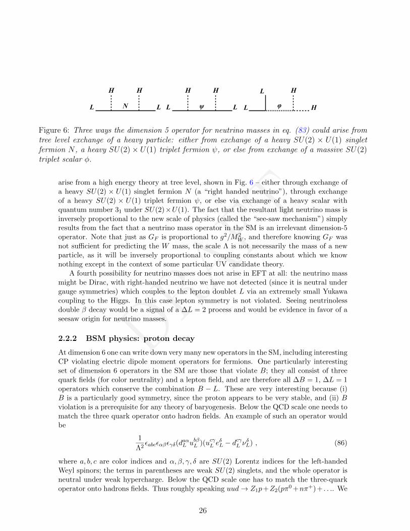
Figure 6: Three ways the dimension 5 operator for neutrino masses in eq. (83) could arise fromtree level exchange of a heavy particle: either from exchange of a heavy SU(2) × U(1) singletfermion N , a heavy SU(2)× U(1) triplet fermion ψ, or else from exchange of a massive SU(2)triplet scalar φ.

arise from a high energy theory at tree level, shown in Fig. 6 – either through exchange ofa heavy SU(2) × U(1) singlet fermion N (a “right handed neutrino”), through exchangeof a heavy SU(2) × U(1) triplet fermion ψ, or else via exchange of a heavy scalar withquantum number 31 under SU(2)×U(1). The fact that the resultant light neutrino mass isinversely proportional to the new scale of physics (called the “see-saw mechanism”) simplyresults from the fact that a neutrino mass operator in the SM is an irrelevant dimension-5operator. Note that just as GF is proportional to g2/M2

W , and therefore knowing GF wasnot sufficient for predicting the W mass, the scale Λ is not necessarily the mass of a newparticle, as it will be inversely proportional to coupling constants about which we knownothing except in the context of some particular UV candidate theory.

A fourth possibility for neutrino masses does not arise in EFT at all: the neutrino massmight be Dirac, with right-handed neutrino we have not detected (since it is neutral undergauge symmetries) which couples to the lepton doublet L via an extremely small Yukawacoupling to the Higgs. In this case lepton symmetry is not violated. Seeing neutrinolessdouble β decay would be a signal of a ∆L = 2 process and would be evidence in favor of aseesaw origin for neutrino masses.

2.2.2 BSM physics: proton decay

At dimension 6 one can write down very many new operators in the SM, including interestingCP violating electric dipole moment operators for fermions. One particularly interestingset of dimension 6 operators in the SM are those that violate B; they all consist of threequark fields (for color neutrality) and a lepton field, and are therefore all ∆B = 1, ∆L = 1operators which conserve the combination B − L. These are very interesting because (i)B is a particularly good symmetry, since the proton appears to be very stable, and (ii) Bviolation is a prerequisite for any theory of baryogenesis. Below the QCD scale one needs tomatch the three quark operator onto hadron fields. An example of such an operator wouldbe

1

Λ2εabcεαβεγδ(d

aαL ubβL )(ucγL e

δL − d

cγL ν

δL) , (86)

where a, b, c are color indices and α, β, γ, δ are SU(2) Lorentz indices for the left-handedWeyl spinors; the terms in parentheses are weak SU(2) singlets, and the whole operator isneutral under weak hypercharge. Below the QCD scale one has to match the three-quarkoperator onto hadrons fields. Thus roughly speaking uud→ Z1p+Z2(pπ0 +nπ+)+ . . .. We

26

DRAFT

can assume that the Z factors are made up of pure numbers times the appropriate powersof the strong interaction scale, such as fπ ' 100 MeV, the pion decay constant. The Z1

term will lead to positron-proton mixing and cannot lead to proton decay, but the Z2 termcan via the processes p→ e+π0, or p→ π+ν. We can make a crude estimate of the width(inverse lifetime) to be

Γ 'M5p

Λ4

1

8π(87)

where I used dimensional analysis to estimate the M5p /Λ

4 factor, assuming that the stronginteraction scale in Z2 as well as powers of momenta from phase space integrals could beapproximated by the proton mass Mp , and I inserted a typical 2-body phase space factorof 1/8π. For a bound on the proton lifetime of τp > 1034 years, this crude estimate givesus Λ & 1016 GeV, not so far off the bound one finds from a more sophisticated calculation.If proton decay is discovered, that will tell us something about the scale of new physics,and then the task will be to construct the full UV theory from what we learn about protondecay, much as the SM was discovered starting from the Fermi theory.

2.3 BSM physics: “partial compositeness”

This next topic does not have to do with accidental symmetry violation, but instead picksup on an interesting feature of the baryon number violating interaction we just discussed,as it suggests a mechanism for quarks and leptons to acquire masses without a Higgs. Inestimating the effects of the dimension six ∆B = 1 operator in the previous section I saidthat the 3-quark operator could be expanded as uud → Z1p + Z2(pπ0 + nπ+) + . . ., andthen focussed on the Z2 term. But what about the Z1 term? By dimensions, Z1 ∼ Λ3

QCD,and so that term gives rise to a peculiar mass term of the form

Λ3QCD

Λ2pe+ h.c. (88)

which allows a proton to mix with a positron, and the anti-proton to mix with the electron.This is not experimentally interesting, but it is an interesting phenomenon for a theorist tocontemplate. Imagine eliminating the Higgs doublet from the SM. The proton would stillget a mass from chiral symmetry breaking in QCD even though the quarks would remainmassless, and due to the above term, and even though there would not be an electron massdirectly from the weak interactions, there would be a above contribution to the proton massdue to the above positron-proton mixing. For the two component system one would havea mass matrix looking something like(

MpΛ3QCD

Λ2

Λ3QCD

Λ2 0

)(89)

and to the extent that Λ ΛQCD we find the mass eigenvalues to be

m1 'Mp , m2 'Λ6QCD

MpΛ4(90)

27

DRAFT

so for Λ = 1016 GeV the positron gets a mass of me ' 10−64 GeV. Yes, this is a ridiculouslysmall mass of no interest, but it is curious that the positron (electron) got a mass at all,without there being any Higgs field! It must be that QCD when QCD spontaneously breakschiral symmetry, it has also broken SU(2) × U(1), without a Higgs, and that this protondecay operator has somehow taken the place of a Higgs Yukawa coupling. Quark fields andQCD has assumed both of the the roles that the Higgs field plays in the SM. Therefore it isworth asking whether this example be modified somehow to obtain more interesting massesfor quarks and leptons?

In a later lecture we will examine how QCD breaks the weak interactions, and how ascaled up version called technicolor, with the analogue of the pion decay constant fπ beingup at the 250 GeV scale instead of 93 MeV, could properly account for the spontaneousbreaking of SU(1) × U(1) without a Higgs. Here I will just comment that such a theorywould be expected to have TeV mass “technibaryons”, which could carry color and charge.With an appropriate dimension 6 operator such as our proton decay operator, but withtechniquarks in place of quarks, and all the standard model fermions in place of the positronfield, in principle one could give masses to all the SM fermions through their mixing with thetechnibaryons. This is the idea of “partial compositeness”, which in its original formulation[1] was not especially useful for model building, but which has become more interesting inthe context of composite Higgs [2] – more about composite Higgs later too.

,

28

DRAFT

2.4 Problems for lecture II

II.1) What is the dimension of the operator φ10 in a d = 2 relativistic scalar field theory?

II.2) One defines the “critical dimension” dc for an operator to be the spacetime dimensionfor which that operator is marginal. How will that operator behave in dimensions d whend > dc or d < dc? In a theory of interacting relativistic scalars, Dirac fermions, and gaugebosons, determine the critical dimension for the following operators:

1. A φ3 interaction;

2. A gauge coupling to either a fermion or a boson through the covariant derivative inthe kinetic term;

3. A Yukawa interaction, φψψ;

4. An anomalous magnetic moment coupling ψσµνFµνψ for a fermion;

5. A four fermion interaction, (ψψ)2.

II.3) Derive the analogue of Fermi’s theory in eq. (72) for tree level Z exchange, expressingyour answer in terms of GF using the fact that M2

Z = M2W / cos2 θw.

II.4) How would one write down an electric dipole operator in QED, and what dimensiondoes it have? What would you have to do to make a gauge invariant electric dipole operatorin the SM that is invariant under the full SU(3)× SU(2)× U(1) gauge symmetry?

II.5) Show that the operator

εαβ (Lαi(σ2σa)ijLβj) (Hk(σ2σ

a)k`H`)

is equivalent up to a factor of two to

εαβ(Lαi(σ2)ijHj)(Lβk(σ2)k`H`)

where α, β are Weyl spinor indices, and i, j, k, ` are the SU(2) gauge group indices. Writedown the two high energy theories that could give rise to the neutrino mass operator as inFig. 6. How do I see that these theories break lepton number by two units?

29

DRAFT

3 EFT and radiative corrections

Up to now we have ignored quantum corrections in our effective theory. A Lagrangiansuch as eq. (57) is what used to be termed a “nonrenormalizable” theory, and to beshunned. The problem was that the theory needs an infinite number of counterterms tosubtract all infinities, and was thought to be unpredictive. In contrast, a “renormalizable”theory contained only marginal and relevant operators, and needed only a finite numberof counterterms, one per marginal or relevant operator allowed by the symmetries. (A“superrenormalizable” theory contained only relevant operators, and was finite beyond acertain order in perturbation theory.) However Wilson changed the view of renormalization.In a perturbative theory, irrelevant operators are renormalized, but stay irrelevant. Onthe other hand, the coefficients of relevant operators are renormalized to take on valuesproportional to powers of the cutoff, unless forbidden by symmetry. Thus in Wilson’s viewthe relevant operators are the problem, since giving them small coefficients requires fine-tuning – unless a symmetry forbids corrections that go as powers of the cutoff. Relevantoperators protected by symmetry include fermion masses and Goldstone boson masses, butfor a general interacting scalar, the natural mass is m2 ' αΛ2 — which means one shouldnever see such scalars in the low energy theory.

In this lecture I discuss the techniques used to create top-down EFTs beyond tree level,as well as an example of an EFT with a marginal interaction with asymptotic freedom andan exponentially small IR scale.

3.1 Matching

I will consider a toy model for UV physics with a light scalar φ and a heavy scalar S :

LUV =1

2

((∂φ)2 −m2φ2 + (∂S)2 −M2S2 − κφ2S

)(91)

The parameter κ has dimension of mass, and I will assume κ .M and that 〈S〉 = 0. Thisis a pretty sill model, but it is useful as an example since the Feynman diagrams are verysimple; never mind that the vacuum energy is unboundedbelow, as one won’t see this inperturbation theory. Suppose we are interested in 2φ → 2φ scattering at energies muchbelow the S mass M , and want to construct the EFT with the heavy S field “integratedout”. Formally:

e−iSeft(φ)

~ =

∫[dS]e−i

S(φ,S)~ (92)

where I use S to denote the action, to distinguish it from the field S. There are good reasonsfor doing so: if you try to compute observables in this theory at some low momentumk << M you are typically going to run into large logarithms of the form ln k2/M2 that willspoil perturbation theory. They are easily taken care of in an EFT where you integrateout S at the scale µ = M , matching the EFT to the full theory to ensure that you arereproducing the same physics. Then within the EFT you run the couplings from µ = M

30

DRAFT

down to µ = k before doing your calculation. The renormalization group running sums upthese large logs for you.

It is convenient to perform the matching in an ~ expansion, meaning that first you makesure that tree diagrams agree in the two theories, as in our derivation of the Fermi theoryof weak interactions from the SM. Then you make sure that the two theories agree at O(~),etc. What sort of graphs does this matching entail, and why is this justified? Consider theoriginal theory, in which ~ only appears in the explicit factor in exp−iS/~, and look at agraph with P propagators, V vertices and E external legs. Euler’s formula tells us thatL = P − V + 1 6. Since ~ enters the path integral through exp(iS/~), every propagatorbrings a power of ~ and every vertex brings a power of ~−1; it follows that a graph isproportional to ~P−V = ~L−1. Since the graph is providing a vertex in Seft/~, the L-loopmatching involves contributions to Left at O(~L). An ~ expansion is always justified whena perturbative expansion is justified. To see that, consider a graph in a theory with a singletype of interaction vertex involving n fields. In this case we have (E+ 2P ) = nV , since oneend of every external line and two ends of every internal line must end on a vertex, andthere must be n lines coming in to each vertex. Putting this together with Euler’s equationwe have V = (2L+E−2)/(n−2), which shows that for a given number of external lines, thenumber of vertices (and hence the power of the coupling constant) grows with the numberof loops, so a loop expansion (or equivalently, an ~ expansion) is justified if a perturbativeexpansion is justified. This can be generalized to a theory with several types of vertices.

So we match the UV theory eq. (91) to the EFT order by order in an ~ expansion with

Left = L0eft + ~L1

eft + ~2L2eft + . . . (93)

What makes this interesting is that we start introducing powers of ~ into the couplingconstants of the EFT, so in the EFT the powers of ~ in a graph can be higher than thenumber of loops; the example below should make this clear. Since the EFT is expressed interms of local operators, the matching also involves performing an expansion in powers ofexternal momenta, with a contribution at pn matching onto an n-derivative operator. Weonly match amplitudes involving light particles on external legs.

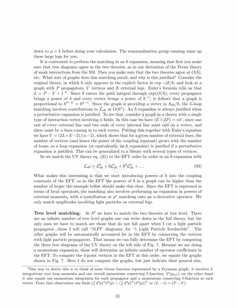
Tree level matching. At ~0 we have to match the two theories at tree level. Thereare an infinite number of tree level graphs one can write down in the full theory, but theonly ones we have to match are those that do not fall apart when I cut a light particlepropagator...these I will call “1LPI” diagrams, for “1 Light Particle Irreducible”. Theother graphs will be automatically accounted for in the EFT by connecting the verticeswith light particle propagators. That means we can fully determine the EFT by computingthe three tree diagrams of the UV theory on the left side of Fig. 7. Because we are doinga momentum expansion, these will determine an infinite number of operator coefficients inthe EFT. To compute the 4-point vertices in the EFT at this order, we equate the graphsshown in Fig. 7. Here I do not compute the graphs, but just indicate their general size,

6One way to derive this is to think of some Green function represented by a Feynman graph: it involves Lintegrations over loop momenta and one overall momentum conserving δ-function, δ4(ptot); on the other handit also equals one momentum integration for each propagator and a momentum conserving δ-function at eachvertex. From that observation one finds (

∫d4p)Lδ4(p) ∼ (

∫d4p)P (δ4(p))V or (L− 1) = (P − V ).

31

DRAFT= +

0

+ +

1

=0 0

0

0

0

0

+ +

+

1

=0

++

+...

Figure 7: Matching at O(~0) between the UV theory and the EFT: on the left, integrating out theheavy scalar S (dark propagator); on the right, all contributions of four-point vertices the treelevel EFT L0

eft. Equating the two sides allows on to solve for this vertices.

= +0

+ +

1

=0 0

0

0

0

0

+ +

+

1

=0

++

+...

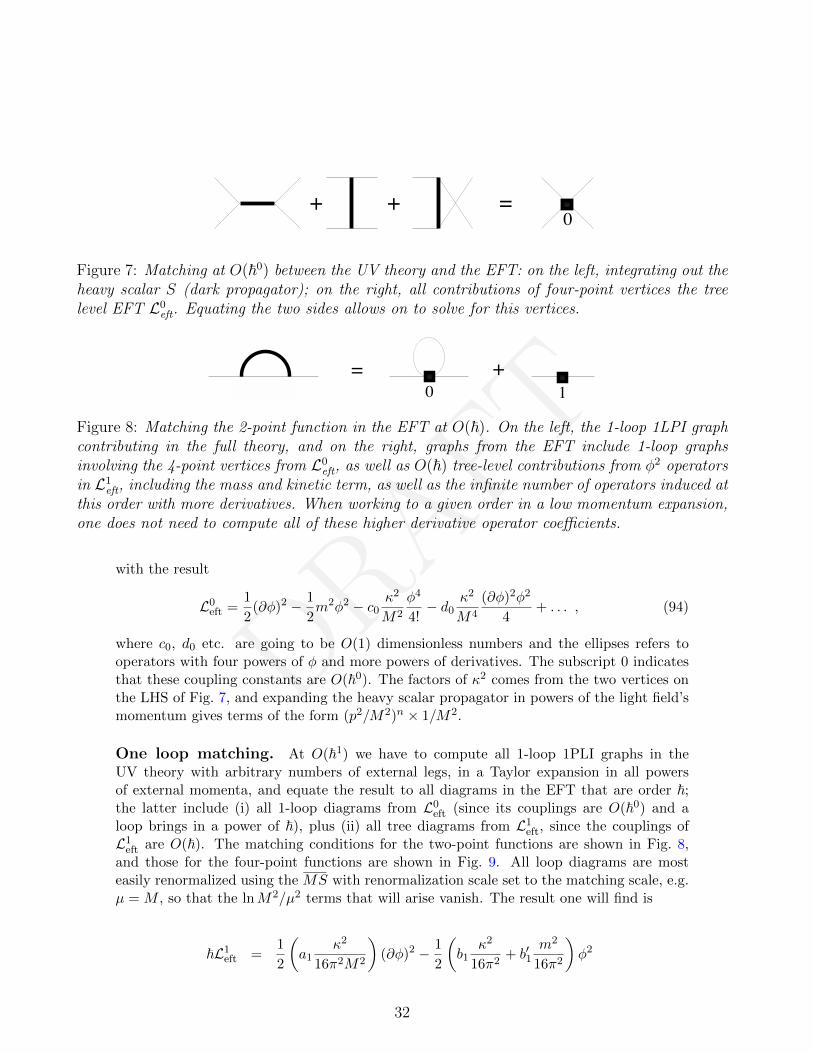
Figure 8: Matching the 2-point function in the EFT at O(~). On the left, the 1-loop 1LPI graphcontributing in the full theory, and on the right, graphs from the EFT include 1-loop graphsinvolving the 4-point vertices from L0

eft, as well as O(~) tree-level contributions from φ2 operatorsin L1

eft, including the mass and kinetic term, as well as the infinite number of operators induced atthis order with more derivatives. When working to a given order in a low momentum expansion,one does not need to compute all of these higher derivative operator coefficients.

with the result

L0eft =

1

2(∂φ)2 − 1

2m2φ2 − c0

κ2

M2

φ4

4!− d0

κ2

M4

(∂φ)2φ2

4+ . . . , (94)

where c0, d0 etc. are going to be O(1) dimensionless numbers and the ellipses refers tooperators with four powers of φ and more powers of derivatives. The subscript 0 indicatesthat these coupling constants are O(~0). The factors of κ2 comes from the two vertices onthe LHS of Fig. 7, and expanding the heavy scalar propagator in powers of the light field’smomentum gives terms of the form (p2/M2)n × 1/M2.

One loop matching. At O(~1) we have to compute all 1-loop 1PLI graphs in theUV theory with arbitrary numbers of external legs, in a Taylor expansion in all powersof external momenta, and equate the result to all diagrams in the EFT that are order ~;the latter include (i) all 1-loop diagrams from L0

eft (since its couplings are O(~0) and aloop brings in a power of ~), plus (ii) all tree diagrams from L1

eft, since the couplings ofL1

eft are O(~). The matching conditions for the two-point functions are shown in Fig. 8,and those for the four-point functions are shown in Fig. 9. All loop diagrams are mosteasily renormalized using the MS with renormalization scale set to the matching scale, e.g.µ = M , so that the lnM2/µ2 terms that will arise vanish. The result one will find is

~L1eft =

1

2

(a1

κ2

16π2M2

)(∂φ)2 − 1

2

(b1

κ2

16π2+ b′1

m2

16π2

)φ2

32

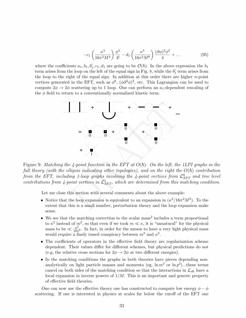
DRAFT

−c1

(κ4

16π2M4

)φ4

4!− d1

(κ4

16π2M6

)(∂φ)2φ2

4+ . . . (95)

where the coefficients a1, b1, b′1, c1, d1 are going to be O(~). In the above expression the b1

term arises from the loop on the left of the equal sign in Fig. 8, while the b′1 term arises fromthe loop to the right of the equal sign. In addition at this order there are higher n-pointvertices generated in the EFT, such as φ6, (φ∂2φ)2, etc. This Lagrangian can be used tocompute 2φ → 2φ scattering up to 1 loop. One can perform an a1-dependent rescaling ofthe φ field to return to a conventionally normalized kinetic term.

= +0

+ +

1

=0 0

0

0

0

0

+ +

+

1

=0

++

+...

Figure 9: Matching the 4-point function in the EFT at O(~). On the left, the 1LPI graphs in thefull theory (with the ellipsis indicating other topologies), and on the right the O(~) contributionfrom the EFT, including 1-loop graphs involving the 4-point vertices from L0

EFT and tree levelcontributions from 4-point vertices in L1

EFT, which are determined from this matching condition.

Let me close this section with several comments about the above example:

• Notice that the loop expansion is equivalent to an expansion in (κ2/16π2M2). To theextent that this is a small number, perturbation theory and the loop expansion makesense.

• We see that the matching correction to the scalar mass2 includes a term proportionalto κ2 instead of m2, so that even if we took m κ, it is “unnatural” for the physicalmass to be κ2

16π2 . In fact, in order for the meson to have a very light physical masswould require a finely tuned conspiracy between m2 and κ2.

• The coefficients of operators in the effective field theory are regularization schemedependent. Their values differ for different schemes, but physical predictions do not(e.g, the relative cross sections for 2φ→ 2φ at two different energies).

• In the matching conditions the graphs in both theories have pieces depending non-analytically on light particle masses and momenta (eg, lnm2 or ln p2)...these termscancel on both sides of the matching condition so that the interactions in Left have alocal expansion in inverse powers of 1/M . This is an important and generic propertyof effective field theories.

One can now use the effective theory one has constructed to compute low energy φ− φscattering. If one is interested in physics at scales far below the cutoff of the EFT one

33

DRAFT

might have to renormalization group improve the answer. For example, in a GUT oneintegrates out particles at the scale MGUT ∼ 1015 GeV and then computes scattering atenergies around 1 GeV. Without RG improvement, the perturbative expansion will involveterms such as α(MGUT) ln 1015 ∼ 0.6. So one eliminates the log by computing in terms ofα(1 GeV). To do that one just needs to compute the β functions in the EFT, ignoring theheavy particles integrated out at MGUT. This procedure requires using a mass-independentrenormalization scheme so one can solve the RG equations. Now since both the protonand top quark exist in the EFT, one risks getting terms such as α(1 GeV) lnmt/mp, forexample, which also isn’t so good if α is the strong coupling. So one can construct a ladderof EFTs, integrating out GUT scale particles at MGUT , the top quark at the scale mt, theW and Z at their mass scale, etc. At each stage in this ladder of EFTs one uses the βfunction appropriate for the light particles that remain as explicit degrees of freedom in theEFT.

Matching computations like this are used for predicting the low energy gauge couplingsin the SM as predicted by Grand Unified Theories (GUTS), integrating out the heavyparticles at the GUT scale MGUT and matching onto the SM as the EFT. At tree levelmatching, the gauge couplings in the EFT at the scale µ = MGUT are equal (when suitablynormalizing the U(1) coupling), and then one runs them down to low energy, each gaugecoupling running in the SM with its own 1-loop β-function. This is the classic calculationof Georgi, Quinn and Weinberg [3] and can be used to predict αs(MZ), since the input aretwo unknowns (the scale MGUT and the GUT gauge coupling g(µ) at µ = MGUT) while theoutput are the three parameter of the SM α, αs(MZ), and sin2 θw. However, if you wantgreater precision you must match the GUT to the EFT at one loop, which generates smalland unequal shifts in the SM gauge coupling at µ = MGUT, and then one scales them downusing the 2-loop β-functions.

3.2 Relevant operators and naturalness

We have seen that a scalar field mass typically gets large additive quantum corrections, sothat in a theory with new physics at scales much larger than the weak scale (e.g. any GUTtheory, and probably any theory with gravity!) it seems unnatural to have light scalars inthe low energy effective theory. This would seem to be a potential problem for the SM,where we know there exists a a Higgs with a weak scale mass, far below the Planck andGUT scales. A natural size for the Higgs mass2 would be α

4πΛ2 where Λ is the cutoff ofthe ET we call the SM. But what is Λ? We have seen that for proton decay and leptonviolation we expect Λ & 1015 GeV; if that is the appropriate Λ to use in the Higgs massestimate, then the SM must be fine-tuned to ∼ 13 orders of magnitude! In fact, the Higgsmass appears not to be fine-tuned only if Λ ∼ 1 TeV – which is one reason to think theLHC might still discover new physics.

Before thinking about what could explain the light Higgs mass, it is interesting to askwhether there are other relevant operaotrs in the SM. Fermion masses in the SM arise fromdimension 4 operators (Yukawa interactions) and are hence marginal above the weak scale.You might think they are relevant below the weak scale, appearing as dimension 3 operatorsmψψ – but that is misleading. Since a fermion mass term breaks the chiral symmetryψ → eiθγ5ψ, a fermion mass can only be renormalized multiplicatively: any divergent

34

DRAFT

diagram must contain chiral symmetry breaking, and hence must be proportional to m.Thus renormalizations of the fermion mass are not additive: (δm ∼ αΛ) but multiplicative:(δm ∼ m ln Λ). Thus light fermion masses are natural since a logarithmic dependence onthe cutoff is very weak and the cutoff may be exponentially larger than the fermion masswithout requiring fine tuning. Similarly, since gauge boson masses break gauge symmetry,they too do not receive additive mass contributions. However there is one other relevantoperator which is problematic: the operator 1, the vacuum energy or cosmological constant.This operator’s coefficient receives additive contributions proportional to Λ4, while we knowthat the cosmological constant needs to be ∼ (10−3 eV)4 to be consistent with cosmologicalobservations – a scale much lower than many known physical scales. A number of newTeV physics scenarios have been proposed to solve or partially solve the Higgs fine-tuning

problem: technicolor, supersymmetry, composite Higgs, extra dimensions... however no onehas found a dynamical theory to explain the small cosmological constant.

It could be that new physics is around the corner, but one has to wonder whether thenaturalness argument isn’t missing something, especially because we see a small cosmolog-ical constant, and we see a light Higgs mass, but we don’t see a host of not-very-irrelevanthigher dimension operators that one might expect to be generated by new physics, andwhose effects we would expect to have seen already if its scale were low. Various ideas havebeen suggested for alternatives to naturalness. One popular one is the anthropic princi-ple, the idea that there are many places in the universe with different parameters, mostof which are “natural” but in which life is impossible. Therefore we exist in those verypeculiar fine-tuned places where life is possible and we shouldn’t worry that it looks like abizarre world. To make these arguments sensible you have to (i) have a UV theory for thepossible values and correlations between parameters (for example: is it possible to find aplace where the up quark is heavy and the down quark is light, or do they have to scaletogether?), as well as a sensible theory for the a priori probability distribution that theytake; then (ii) one has to have a good understanding about how these parameters affect ourexistence. I have only seen two examples where these two criteria are met at all: anthropicarguments for the cosmological constant [4], and anthropic arguments for the axion in aninflationary universe (see [5] and references therein). And in fact, the anthropic solution isthe only plausible explanation for the small cosmological constant that has been proposed.I will return to the anthropic axion in my last lecture.

Another idea is that the world is fine-tuned because of its dynamical evolution. Whereasa creationist might say that human eye is a miraculous finely-tuned apparatus, the evolu-tionist says it is the product of a billion years of evolution. Perhaps the light Higgs is due tosome dynamical path that the universe has taken since the Big Bang? A very creative ideaalong these lines recently appeared in [6], again involving the axion. See also the parableI have reprinted below (but will not include in my lecture) from my 1997 TASI lectures; Iwrote that after being at a conference where I thought that SUSY advocates were beingway too smug about the theory!

3.3 Aside – a parable from TASI 1997

I used to live in San Diego near a beach that had high cliffs beside it. The cliffs werecomposed of compressed sand, and sand was always sprinkling down to the beach below.

35

DRAFT

At the base of these cliffs there was always a little ramp of sand. One day I was walkingdown the beach with a physicist friend of mine, and she remarked on the fact that each ofthese ramps of sand was at precisely the same angle.

“How peculiar!” she said, and I had to agree, but thought no further of it. However,she had a more inquiring mind than I, and called me up that evening:

“I’ve been conducting an experiment,” she said. “I take a box of sand and tilt it until itavalanches, which occurs at an angle θc. You won’t believe it, but θc is precisely the sameangle as the ramps of sand we saw at the beach! Isn’t that amazing?”

“Indeed,” I said. “Apparently someone has performed the same experiment as you, andhas sent someone out to adjust all the sand piles to that interesting angle. Perhaps it’s theMaster’s project of some Fine Arts student.”

“That’s absurd!” she said. “I could believe it if the artist did this once, but just think— the wind is always blowing sand onto some piles and off of other piles! The artist wouldhave to fix the piles continuously, day and night!”

As unlikely as this sounded, I had to insist that there seemed to be no alternative.However, the next morning when we met again, my friend was jubilant.

“I figured out what is going on!” she exclaimed. “I have deduced the existence of swind.Every time the wind blows and moves the sand, swind blows and moves it back! I call this‘Swindle Theory’. ”

“That’s absurd!” I exclaimed. “Wind is made of moving molecules, what in the worldis swind made of, and why haven’t we seen it?”

“Smallecules,” she replied, “they’re too small to see.”“But you still need the art student to come by in the beginning and fix the sand at

precisely the angle θc, right?” I asked.“True”“So why should I believe in Swindle Theory? You’ve hardly explained anything!”“Well look,” she retorted, “see how beautiful the Navier-Stokes equations become when

generalized to include swind?”Indeed, the equations were beautiful, so beautiful that I felt compelled to believe in

Swindle Theory, although I occasionally still have my doubts...

3.4 Landau liquid versus BCS instability

We have discussed irrelevant operators and rare symmetry violating processes; relevantoperators and the naturalness problem; let us now turn to the fascinating case of asymp-totically free marginal interactions.

In our discussion of 2D quantum mechanics we encountered asymptotic freedom and thedynamical generation of an exponentially small scale in the IR. This is a possibility in theo-ries with marginal interactions that are pushed into relevancy by small radiative corrections;however it is known that for relativistic QFTs it only actually happens in nonabelian gaugetheories – the most famous example being QCD. Asymptotic freedom explains why ΛQCD

is naturally so much smaller than the GUT or Planck scales. However, the same physics isresponsible for the large Cooper pairs found in superconducting materials, which I describehere, following the work of Polchinski [7]. I like this example because it emphasizes that

36

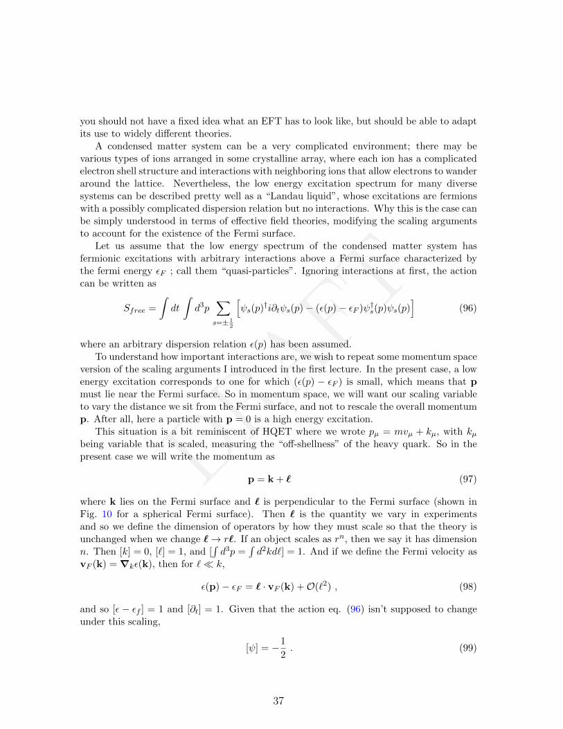
DRAFT

you should not have a fixed idea what an EFT has to look like, but should be able to adaptits use to widely different theories.

A condensed matter system can be a very complicated environment; there may bevarious types of ions arranged in some crystalline array, where each ion has a complicatedelectron shell structure and interactions with neighboring ions that allow electrons to wanderaround the lattice. Nevertheless, the low energy excitation spectrum for many diversesystems can be described pretty well as a “Landau liquid”, whose excitations are fermionswith a possibly complicated dispersion relation but no interactions. Why this is the case canbe simply understood in terms of effective field theories, modifying the scaling argumentsto account for the existence of the Fermi surface.

Let us assume that the low energy spectrum of the condensed matter system hasfermionic excitations with arbitrary interactions above a Fermi surface characterized bythe fermi energy εF ; call them “quasi-particles”. Ignoring interactions at first, the actioncan be written as

Sfree =

∫dt

∫d3p

∑s=± 1

2

[ψs(p)

†i∂tψs(p)− (ε(p)− εF )ψ†s(p)ψs(p)]

(96)

where an arbitrary dispersion relation ε(p) has been assumed.To understand how important interactions are, we wish to repeat some momentum space

version of the scaling arguments I introduced in the first lecture. In the present case, a lowenergy excitation corresponds to one for which (ε(p) − εF ) is small, which means that pmust lie near the Fermi surface. So in momentum space, we will want our scaling variableto vary the distance we sit from the Fermi surface, and not to rescale the overall momentump. After all, here a particle with p = 0 is a high energy excitation.

This situation is a bit reminiscent of HQET where we wrote pµ = mvµ + kµ, with kµbeing variable that is scaled, measuring the “off-shellness” of the heavy quark. So in thepresent case we will write the momentum as

p = k + ` (97)

where k lies on the Fermi surface and ` is perpendicular to the Fermi surface (shown inFig. 10 for a spherical Fermi surface). Then ` is the quantity we vary in experimentsand so we define the dimension of operators by how they must scale so that the theory isunchanged when we change `→ r`. If an object scales as rn, then we say it has dimensionn. Then [k] = 0, [`] = 1, and [

∫d3p =

∫d2kd`] = 1. And if we define the Fermi velocity as

vF (k) = ∇kε(k), then for ` k,

ε(p)− εF = ` · vF (k) +O(`2) , (98)

and so [ε − εf ] = 1 and [∂t] = 1. Given that the action eq. (96) isn’t supposed to changeunder this scaling,

[ψ] = −1

2. (99)

37

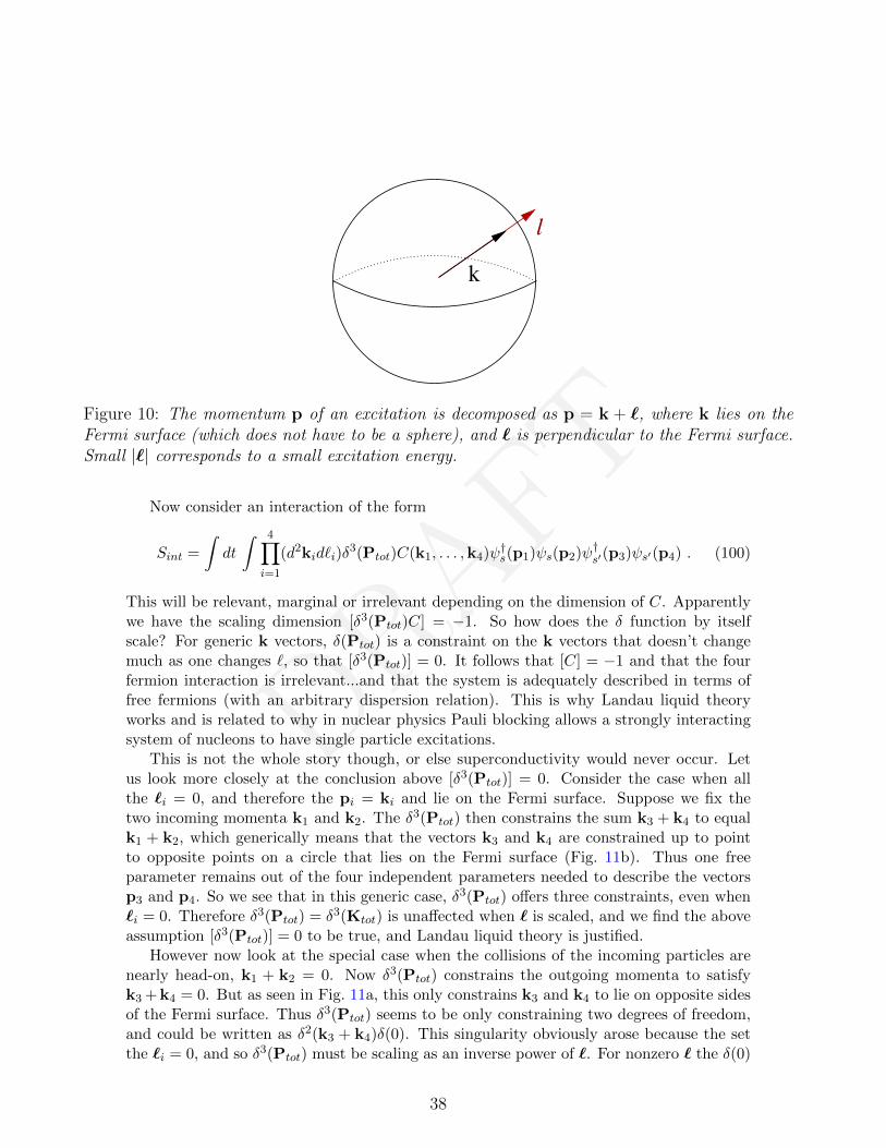
DRAFT

l

k

Figure 10: The momentum p of an excitation is decomposed as p = k + `, where k lies on theFermi surface (which does not have to be a sphere), and ` is perpendicular to the Fermi surface.Small |`| corresponds to a small excitation energy.

Now consider an interaction of the form

Sint =

∫dt

∫ 4∏i=1

(d2kid`i)δ3(Ptot)C(k1, . . . ,k4)ψ†s(p1)ψs(p2)ψ†s′(p3)ψs′(p4) . (100)

This will be relevant, marginal or irrelevant depending on the dimension of C. Apparentlywe have the scaling dimension [δ3(Ptot)C] = −1. So how does the δ function by itselfscale? For generic k vectors, δ(Ptot) is a constraint on the k vectors that doesn’t changemuch as one changes `, so that [δ3(Ptot)] = 0. It follows that [C] = −1 and that the fourfermion interaction is irrelevant...and that the system is adequately described in terms offree fermions (with an arbitrary dispersion relation). This is why Landau liquid theoryworks and is related to why in nuclear physics Pauli blocking allows a strongly interactingsystem of nucleons to have single particle excitations.

This is not the whole story though, or else superconductivity would never occur. Letus look more closely at the conclusion above [δ3(Ptot)] = 0. Consider the case when allthe `i = 0, and therefore the pi = ki and lie on the Fermi surface. Suppose we fix thetwo incoming momenta k1 and k2. The δ3(Ptot) then constrains the sum k3 + k4 to equalk1 + k2, which generically means that the vectors k3 and k4 are constrained up to pointto opposite points on a circle that lies on the Fermi surface (Fig. 11b). Thus one freeparameter remains out of the four independent parameters needed to describe the vectorsp3 and p4. So we see that in this generic case, δ3(Ptot) offers three constraints, even when`i = 0. Therefore δ3(Ptot) = δ3(Ktot) is unaffected when ` is scaled, and we find the aboveassumption [δ3(Ptot)] = 0 to be true, and Landau liquid theory is justified.

However now look at the special case when the collisions of the incoming particles arenearly head-on, k1 + k2 = 0. Now δ3(Ptot) constrains the outgoing momenta to satisfyk3 + k4 = 0. But as seen in Fig. 11a, this only constrains k3 and k4 to lie on opposite sidesof the Fermi surface. Thus δ3(Ptot) seems to be only constraining two degrees of freedom,and could be written as δ2(k3 + k4)δ(0). This singularity obviously arose because the setthe `i = 0, and so δ3(Ptot) must be scaling as an inverse power of `. For nonzero ` the δ(0)

38

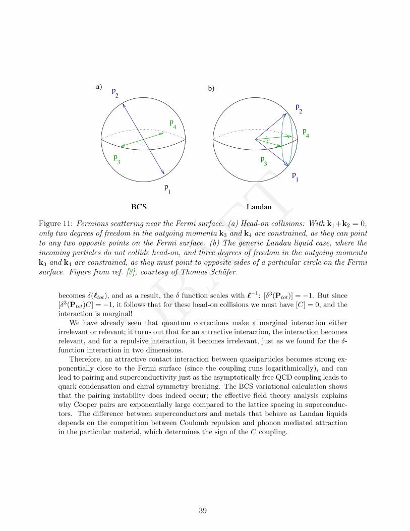
DRAFT

p1

p1

p2

p4

p3 p

3

p4

p2

BCS Landau

a) b)

Figure 11: Fermions scattering near the Fermi surface. (a) Head-on collisions: With k1 +k2 = 0,only two degrees of freedom in the outgoing momenta k3 and k4 are constrained, as they can pointto any two opposite points on the Fermi surface. (b) The generic Landau liquid case, where theincoming particles do not collide head-on, and three degrees of freedom in the outgoing momentak3 and k4 are constrained, as they must point to opposite sides of a particular circle on the Fermisurface. Figure from ref. [8], courtesy of Thomas Schafer.

becomes δ(`tot), and as a result, the δ function scales with `−1: [δ3(Ptot)] = −1. But since[δ3(Ptot)C] = −1, it follows that for these head-on collisions we must have [C] = 0, and theinteraction is marginal!

We have already seen that quantum corrections make a marginal interaction eitherirrelevant or relevant; it turns out that for an attractive interaction, the interaction becomesrelevant, and for a repulsive interaction, it becomes irrelevant, just as we found for the δ-function interaction in two dimensions.

Therefore, an attractive contact interaction between quasiparticles becomes strong ex-ponentially close to the Fermi surface (since the coupling runs logarithmically), and canlead to pairing and superconductivity just as the asymptotically free QCD coupling leads toquark condensation and chiral symmetry breaking. The BCS variational calculation showsthat the pairing instability does indeed occur; the effective field theory analysis explainswhy Cooper pairs are exponentially large compared to the lattice spacing in superconduc-tors. The difference between superconductors and metals that behave as Landau liquidsdepends on the competition between Coulomb repulsion and phonon mediated attractionin the particular material, which determines the sign of the C coupling.

39

DRAFT

3.5 Problems for lecture III

III.1) A small fermion mass can be considered natural, in contrast to a small scalar mass.This has to do with the fact that if a fermion becomes massless, usually the symmetry of thetheory is enhanced by a U(1) chiral symmetry ψ → eiαγ5ψ. Thus at m = 0, there cannotbe any renormalization of the fermion mass. A corollary is that at nonzero mass m, anyrenormalization must be proportional to m. Can you explain why this makes the fermionmass behave like a marginal operator rather than a relevant one? Can you construct anexample of a theory where it is not natural to have a light fermion?

40

DRAFT

4 Chiral perturbation theory

4.1 Chiral symmetry in QCD

QCD is the accepted theory of the strong interactions. At large momentum transfer, asin deep inelastic scattering processes and the decays of heavy particles such as the Z, thetheory is perturbative due to asymptotic freedom. The flip side is that in the infrared,the theory becomes nonperturbative. This is good in the sense that we know that thelight hadrons don’t look at all like a collection of quarks weakly interacting via gluonexchange. But it does mean that QCD is not of much help in quantitatively understandingthis phenomenology without resorting to lattice QCD and a computer. However, there doesexist an effective field theory which is very powerful for treating analytically the interactionsof the lightest hadrons, the pseudoscalar octet, consisting of the π, K, K and η.

The reason that the pseudoscalar octet mesons are lighter is because they are the pseudo-Goldstone bosons (PGBs) that arise from the spontaneous breaking of an approximatesymmetry in QCD.

Consider the QCD Lagrangian, keeping only the three lightest quarks, u, d and s:

L =3∑i=1

(qii /Dqi −miqiqi

)− 1

2TrGµνG

µν , (101)

where Dµ = ∂µ + igAµ is the covariant derivative, Aµ = AaµTa are the eight gluon fieldswith Ta being SU(3) generators in the 3 representation, and Gµν being the gluon fieldstrength. Note that if I write the kinetic term in terms of right-handed and left-handedquarks, projected out by (1± γ5)/2 respectively, then the kinetic term may be written as∑

i

qii /Dqi =∑i

(qLii /DqLi + qRii /DqRi

). (102)

This term by itself evidently respects a U(3)L ×U(3)R symmetry, where I rotate the threeflavors of left-handed and right-handed quarks by independent unitary matrices. One com-bination of these transformations, the U(1)A transformation where qi → eiαγ5qi is in factnot a symmetry of the quantum theory, due to anomalies; it is a symmetry of the action butnot of the measure of the path integral. This leaves us with a U(1)V × SU(3)L × SU(3)Rsymmetry. The U(1)V is just baryon number, under which both left- and right-handedquarks of all flavors pick up a common phase. The remaining SU(3)L × SU(3)R symme-try, under which qLi → LijqLj and qRj → RijqRj , where R and L are independent SU(3)matrices, is called “chiral symmetry”.

SU(3)L × SU(3)R is not an exact symmetry of QCD, however. The quark mass termsmay be written as

∑i

miqiqi =∑i,j

qRiMijqLj + h.c. , M =

mu

md

ms

, (103)

where the quark masses mi are called “current masses”, not to be confused with the muchbigger constituent quark masses in the quark model. Since the mass term couples left- andright-handed quarks, it is not invariant under the full chiral symmetry. Several observations:

41

DRAFT

• Note that if the mass matrix M were a dynamical field, transforming under SU(3)L×SU(3)R as

M → RML† , (104)

then the Lagrangian would be chirally invariant. Thinking of the explicit breakingof chiral symmetry as being due to spontaneous breaking due to a field M whichtransforms as above makes it simple to understand how M must appear in the effectivetheory, which will have to be chirally invariant given the above transformation. Thisis called treating M as a “spurion”.

• The symmetry is broken to the extent that M 6= RML†. Since mu and md are muchsmaller than ms, SU(2)L × SU(2)R is not broken as badly as SU(3)L × SU(3)R;

• If all three quark masses were equal but nonzero, then QCD would respect an exactSU(3)V ⊂ SU(3)L × SU(3)R symmetry, where one sets L = R. This is the SU(3)symmetry of Gell-Mann.

• Since md−mu is small, SU(2)V ⊂ SU(3)V , where L = R and they act nontrivially onlyon the u and d quarks, is quite a good symmetry...also known as isospin symmetry.

• Independent vectorlike phase rotations of the three flavors of quarks are exact sym-metries...these three U(1) symmetries are linear combinations of baryon number, I3

isospin symmetry, and Y (hypercharge). The latter two are violated by the weakinteractions, but not by the strong or electromagnetic forces.

We know that this still is not the whole story though. An added complication is thatthe QCD vacuum spontaneously breaks the chiral SU(3)L × SU(3)R symmetry down toGell-Mann’s SU(3)V via the quark condensate:

〈0|qRjqLi|0〉 = Λ3δij , (105)

which transforms as a (3, 3) under SU(3)L × SU(3)R. Here Λ has dimensions of mass. Ifone redefines the quark fields by a chiral transformation, the Kronecker δ-function abovegets replaced by a general SU(3) matrix,

〈0|qRjqLi|0〉 → Lim〈0|qRnqLm|0〉R†nj = Λ3 (LR†)ij ≡ Λ3 Σij . (106)

Note that Σ is an SU(3) matrix. If L = R (an SU(3)V transformation, Gell-Mann’s SU(3)),then Σij = δij which shows that the condensate leaves unbroken the SU(3)V symmetry.For L 6= R, Σij represents a different vacuum from eq. (105), and if it wasn’t for the explicitbreaking of SU(3)L×SU(3)R by quark masses in the QCD Lagrangian, these two differentvacua would be degenerate. By Goldstone’s theorem therefore, there would have to be eightexact Goldstone bosons — one for each of the eight broken generators — correspondingto long wavelength, spacetime dependent rotations of the condensate. We will parametrizethese excitations by replacing

Σ→ Σ(x) ≡ e2iπ(x)/f , π(x) = πa(x)Ta (107)

where the Ta are the SU(3) generators (a = 1, . . . , 8) in the defining representation nor-malized to

TrTaTb =1

2δab , (108)

42

DRAFT

f is a parameter with dimension of mass which we will relate to the pion decay constantfπ, and the πa are eight mesons transforming as an octet under SU(3)V . This meson octetcorresponds to long wavelength excitations of the vacuum, and the interactions of thesemesons are represented by the chiral Lagrangian; it is an EFT because the mesons are thelightest excitations of QCD, and we ignore all heavier states, such as the ρ meson. In orderto construct this theory we are going to be guided by symmetry: under an SU(3)L×SU(3)Rtransformation we have

Σ(x)→ LΣ(x)R† , (109)

for arbitrary SU(3) matrices L and R, and we are going to require that the chiral Lagrangianbe invariant under this transformation. What makes the story interesting is that SU(3)L×SU(3)R is not an exact symmetry, but i broken by nonzero quark masses and by the electriccharges of the quarks, and we will have to incorporate those effects.

If you are somewhat overwhelmed by this amazing mix of symmetries that are gauged,global, exact, approximate, spontaneously broken and anomalous (and each individual sym-metry has usually more than one of these attributes at the same time), rest assured that ittook a decade and many physicists to sort it all out (the 1960’s).

4.2 Quantum numbers of the meson octet

It is useful to use the basis for SU(3) generators Ta = 12λa, where λa are Gell Mann’s eight

matrices. The meson matrix π ≡ πaTa appearing in the exponent of Σ is a traceless 3× 3matrix. We know that under and SU(3)V transformation L = R = V ,

Σ→ V ΣV † = e2iV πV †/f , (110)

implying that under SU(3)V the mesons transform as an octet should, namely

π → V πV † . (111)

Then by restricting V to be an I3 (T3) or a Y (T8) rotation we can read off the quantumnumbers of each element of the π matrix and identify them with real particles:

π =1√2

π0√

2+ η√

6π+ K+

π− − π0√

2+ η√

6K0

K− K0 − 2η√6

(112)

An easy way to understand the normalization is to check that

Tr(ππ) =1

2

∑a

(πa)2 =

1

2(π0)2 +

1

2η2 + π+π− +K+K− +K0K0 . (113)

which is a manifestly SU(3)V invariant operator.

43

DRAFT

4.3 The chiral Lagrangian

4.3.1 The leading term and the meson decay constant

We are now ready to write down the effective theory of excitations of the chiral condensate(the chiral Lagrangian), ignoring all the other modes of QCD. This is analogous to thequantization of rotational modes of a diatomic molecule, ignoring the vibrational modes.We are guided by two basic principles of effective field theory: (i) The chiral Lagrangianmust exhibit the same approximate chiral symmetry as QCD, which means that it must beinvariant under Σ→ LΣR† for arbitrary SU(3)L × SU(3)R matrices L, R. We will also beable to incorporate symmetry breaking effects by including the matrix M , requiring that thechiral Lagrangian be invariant under the chiral symmetry if M were to transform as in eq.(104). (ii) The other principle is that the effective theory be an expansion of local operatorssuppressed by powers of a cutoff Λ, which is set by the scale of physics we are ignoring,such as the ρ, K∗, ω, and η′ mesons (with masses mρ = 770 MeV, mK∗ = 892 MeV,mω = 782 MeV and mη′ = 958 MeV). In practice, the cutoff seems to be at Λ ' 1 GeV inmany processes. Our calculations will involve an expansion in powers of momenta or mesonmasses divided by Λ. This cutoff is to be compared with mπ± = 140 MeV, mK+ = 494 MeVand mη = 548 MeV. For purely mesonic processes, meson masses always appear squared,which helps. Nevertheless, one can surmise that chiral perturbation theory will work farbetter for pions than kaons or the η. This is a reflection of the fact that SU(2)L × SU(2)Ris a much better symmetry of QCD than SU(3)L × SU(3)R.

The lowest dimension chirally symmetric operator we can write down is

L0 =f2

4Tr∂Σ†∂Σ = Tr∂π∂π +

1

3f2Tr[∂π,π]2 + . . . (114)

Note that the f2/4 prefactor is fixed by requiring that the mesons have canonically normal-ized kinetic terms. Thus we have an infinite tower of operators involving a single unknownparameter, f . From the above Lagrangian, it would seem that the only way to determinef is by looking at ππ scattering. However there is a better way: by looking at the chargedpion decay π → µν. This occurs through the “semi-leptonic” weak interaction eq. (72),namely the operator

1√2GFVud (uγµ(1− γ5)d) (µγµ(1− γ5)νµ) + h.c. (115)

The matrix element of this operator sandwiched between |µν〉 and 〈π| factorizes, and theleptonic part is perturbative. We are left with the nonperturbative part,

〈0|uγµ(1− γ5)d|π−(p)〉 ≡ i√

2 fπpµ . (116)

The pion decay constant fπ is determined from the charged pion lifetime to be fπ =92.4± .25 MeV.

Even though QCD is nonperturbative, we can easily match this charged current operatoronto an operator in the chiral Lagrangian. That is because we can write

uγµ(1− γ5)d = 2(jµL1 + ijµL2

), (117)

44

DRAFT

where jµLa are the eight SU(3)L currents

jµLa ≡ qγµ

(1− γ5

2

)Taq . (118)

To compute these currents in the effective theory is easy, since we know that under SU(3)Ltransformations Σ → LΣ, or δLaΣ = iTaΣ, and can just compute the left-handed currentsfrom the Lagrangian L0 in eq. (114) using Noethers theorem. The result is:

jµLa = −if2

2TrTaΣ

†∂µΣ = fTrTa∂µπ +O(π2) . (119)

In particular,

2(jµL1 + ijµL2

)= 2f Tr

0 1 00 0 00 0 0

∂µπ +O(π2) =√

2f∂µπ− +O(π2) , (120)

were I made use of eq. (112). Comparing this equation with eq. (116) we see that to thisorder,

f = fπ = 93 MeV . (121)

In general it is not possible to exactly match quark operators with operators in thechiral Lagrangian; it was possible for the semileptonic decays simply because the weakoperator factorized into a leptonic matrix element and a hadronic matrix element of anSU(3)L symmetry current. For a purely hadronic weak decay, such as K → ππ the fourquark operator cannot be factorized, and matching to operators in the chiral Lagrangianinvolves coefficients which can only be computed on a lattice. Even for these processes thechiral Lagrangian can be predictive, relating weak decays with different numbers of mesonsin the final state.

4.3.2 Explicit symmetry breaking

Up to now, I have only discussed operators in the chiral Lagrangian which are invariant.Note that that there are no chirally invariant operators which do not have derivatives (otherthan the operator 1). For example, one cannot write down a chirally invariant mass term forthe pions. Recall that without explicit chiral symmetry breaking in the QCD Lagrangian,there would be an infinite number of inequivalent degenerate vacua corresponding to dif-ferent constant values of the matrix Σ; therefore the energy (and the Lagrangian) can onlyhave operators which vanish when Σ is constant, up to an overall vacuum energy indepen-dent of Σ. In fact, rotating Σ → Σ′ = Σ + idθa Ta Σ is an exact symmetry of the theory(SU(3)L), and corresponds to shifting the pion fields πa → πa+dθa f/2+O(π2). Derivativeinteractions are a result of this shift symmetry. (In the literature, this is called a nonlinearlyrealized symmetry, which is to say, a spontaneously broken symmetry). A theory of mass-less particles with nontrivial interactions at zero momentum transfer (such as QCD) wouldsuffer severe infrared divergences, and so if the interactions had not been purely derivative,the theory would either not make sense, or would become nonperturbative like QCD.

45

DRAFT

This all changes when explicit chiral symmetry breaking is included. Now not all vacuaare equivalent, the massless Goldstone bosons become massive “pseudo-Goldstone bosons”(PGBs), and acquire nonderivative interactions. In pure QCD, the only sources of explicitchiral symmetry breaking are instantons (which explicitly break the U(1)A symmetry, andthe quark mass matrix. Electromagnetic interactions also introduce chiral symmetry break-ing, as do weak interactions.

Quark masses. To include the effect of quark masses, we need to include the massmatrix M , recalling that if it transformed as in eq. (104), then the theory would have tobe invariant. Just as with derivatives, each power of M will be accompanied by 1/Λ. Theleading operator we can write down is

LM = Λ2f2

(c

2

1

ΛTrMΣ + h.c.

)≡ 1

2f2Tr(ΛM)Σ + h.c. , (122)

where c is an unknown dimensionless coefficient, and I defined

cΛ ≡ Λ = O(Λ) . (123)

Expanding to second order in the π, I get

LM = −m2ππ

+π− −m2K+K

+K− −m2K0K

0K0 − 1

2

(π0 η

)i

[M2

0

]ij

(π0

η

)j

, (124)

with

m2π = Λ(mu +md) , m2

K+ = Λ(mu +ms) , m2K0 = Λ(md +ms) , (125)

and

M20 = Λ

((mu +md) (mu −md)(mu −md)

13(mu +md + 4ms)

)(126)

Note that (i) the squares of the meson masses are proportional to quark masses; (ii) π0− ηmixing is isospin breaking and proportional to (mu − md); (iii) expanding in powers of(mu − md), m

2η and m2

π0 are given by the diagonal entries of M20 , up to corrections of

O((mu −md)

2); (iv) we cannot directly relate quark and meson masses because of the

unknown coefficient Λ.Ignoring isospin breaking due to electromagnetism and the difference mu 6= md, the

masses we have computed obey the Gell-Mann Okuba formula

3m2η +m2

π = 4m2K . (127)

The two sides of the above equation are satisfied experimentally to better than 1% accuracy.

46

DRAFT

Electromagnetism. To include electromagnetism into the chiral Lagrangian, we haveto first go back to QCD and ask what currents out of our eight jµLa and jµRa couple to thephoton. That is easy: the photon couples to the electromagnetic current which can bewritten as

Jµem = eqγµPLQLq + eqγµPRQRq , QL = QR =

23−1

3−1

3

, (128)

a simple linear combination of octet currents. So symmetry determines the covariant deriva-tive in the chiral Lagrangian to be

DµΣ = ∂µΣ− ieAµ (QLΣ− ΣQR) (129)

since Σ→ LΣR† under SU(3)L×SU(3)R. Note that when we set the Σ field to its vacuumvalue, Σ = 1, the photon term drops out of the covariant derivative, which is to say that thevacuum does not break electromagnetism spontaneously. Also note that the QL,R matricesare SU(3)L × SU(3)R spurions: in order to have unbroken chiral symmetry we would needDµΣ to have the transformation property DµΣ→ LDµΣR† when Σ→ LΣR†, which wouldrequire the transformation properties

QL → L†QLL† , QR → RQRR

† , (130)

which is to say that QL transforms as part of the adjoint (octet) of SU(3)L and a singletunder SU(3)R, and conversely for QR. We would have muddled this if we had not takencare to distinguish QL,R from each other from the start, even though for the photon thenend up being the same matrix.

If we now want to compute the electromagnetic contribution to the π+−π0 mass splittingto order α we naturally look at the two one-loop diagrams we encounter in scalar QED.These are quadratically divergent, which means they need a counter term which wouldcontribute to the pion mass2 approximately ∼ α/4πΛ2 ∼ e2f2. From the transformationproperties eq. (130) we see that we can add such a counter term operator to the chiralLagrangian of the form

Lα = ξf4 α

4πTrQLΣQRΣ† (131)

where would would expect c = O(1), but which needs to be fit to data or computed usinglattice QCD. If we use the MS scheme in Landau gauge, them the 1-loop diagrams vanishand we are left only with the direct contribution from the above operator in . Expandingit to second order in meson fields we get

Lα = −ξf4e2 2

f2TrQL [π, [π, QR]] = −2ξe2f2

(π+π− +K+K−

)(132)

a simple result which says that the meson mass2 gets shifted by a constant amount propor-tional to its charge squared.

Thus to leading order in α and the quark masses, our formula for the meson massestake the form

m2π+ = Λ(mu +md) +

α

4π∆2 , m2

K+ = Λ(mu +ms) +α

4π∆2 , (133)

47

DRAFT

with the neutral particle masses unchanged, where ∆2 = 2ξ(4πf)2 is a parameter whosevalue we cannot predict. Following Weinberg, however, we can manipulate our formulas tomake predictions for ratios of combinations of meson masses chosen so that the unknownparameters ∆ and Λ drop out:

(m2K+ −m2

K0)− (m2π+ −m2

π0)

m2π0

=mu −md

mu +md,

3m2η −m2

π0

m2π0

=4ms

mu +md. (134)

Plugging in the measured meson masses, these formulas let us determine the ratios of quarkmasses in QCD:

mu

md' 1

2,

md

ms' 1

20. (135)

To specify the quark masses themselves, one must perform a lattice QCD calculation anddesignate a renormalization scheme. Lattice simulations typically find ms renormalized atµ = 2 GeV in the MS scheme lies in the 80− 100 MeV range, from which one infers fromthe above ratios md ∼ 5 MeV, mu ∼ 2.5 MeV in the same scheme. Evidently most of themass of baryons and vector mesons does not come from the intrinsic masses of the quarks.

4.4 Loops and power counting

What makes the chiral Lagrangian an EFT and not just another model of the stronginteractions is that it consists of all local operators consisted with the symmetries of QCD,and that there exists a power counting scheme that allows one to work to a given order, andto be able to make a reliable estimate of the errors arising from neglecting the subsequentorder.

Beyond the leading term is an infinite number of chirally invariant operators one canwrite down which are higher powers in derivatives, as well as operators with more insertionsof the quark mass matrix M . The derivative expansion is in powers of ∂/Λ, where Λ isthe “chiral symmetry breaking scale”, which should be O(1 GeV), since that is the massscale of all the lowest hadronic resonances not included in the theory. This power countingis consistent with the leading operator eq. (114), if you consider the chiral Lagrangian tohave a prefactor of Λ2f2, then even in the leading operator derivatives enter as ∂/Λ:

L0 = Λ2f2

(1

4Λ2Tr ∂Σ† ∂Σ

). (136)

Since we have found that meson octet masses scale as m2π ' (ΛM), and since for on-shell

pions p2 ∼ m2, it follows that one insertion of the quark mass matrix is equivalent totwo derivatives in the effective field theory expansion. This leads us to write the chiral La-grangian as a function of (∂/Λ) and ΛM/Λ2. Including electromagnetism is straightforwardas well: since a derivative ∂Σ becomes a covariant derivative DµΣ = ∂µΣ − ieAµ [Q,Σ],and so the covariant derivative should come with a 1/Λ factor, and hence the photon fieldenters as eAµ/Λ. Operators arising from electromagnetic loops involve two insertions of thequark charge matrix Q in the proper way, along with a loop factor α/(4π). Therefore the

48

DRAFT

action for the chiral theory takes the form

S =

∫d4xΛ2f2L

[Σ, Dµ/Λ, ΛM/Λ2, (α/4π)Q2

], (137)

where L is a dimensionless sum of all local, chirally invariant operators (treating M and Qas spurions), where the coefficient of each term (except L0) is preceded by a dimensionlesscoefficient to be fit to experiment... which we expect to be O(1), but which may occasionallysurprise us! That last assumption is what allows one to estimate the size of higher ordercorrections.

It should be clear now in what sense the u, d and s are light quarks and can be treatedin chiral perturbation theory, while the c, b and t quarks are not: whether the quarksare light or heavy is relative to the scale Λ, namely the mass scale of resonances in QCD.Since the c has a mass ∼ 1.5 GeV there is no sensible way to talk about an approximateSU(4)×SU(4) chiral symmetry and include D, Ds and ηc mesons in our theory of pseudo-Goldstone bosons7 Of course, you might argue that the strange quark is sort of heavy andshould be left out as well, but if we don’t live dangerously sometimes, life is too boring.

4.4.1 Subleading order: the O(p4) chiral Lagrangian

It is a straightforward exercise to write down subleading operators of the chiral Lagrangian.These are operators of O(p4), O(p2M) and O(M2), where M is the quark mass matrix.This was first done by Gasser and Leutwyler, and their choice for the set of operators hasbecome standard:

Lp4 = L1

(Tr(∂µΣ†∂µΣ

))2

+L2Tr(∂µΣ†∂νΣ

)Tr(∂µΣ†∂νΣ

)+L3Tr

(∂µΣ†∂µΣ∂νΣ†∂νΣ

)+L4Tr

(∂µΣ†∂µΣ

)Tr (χΣ + h.c.)

+L5Tr((∂µΣ†∂µΣ

)(χΣ + h.c.)

)+L6 (Tr (χΣ + h.c.))2

+L7 (Tr (χΣ− h.c.))2

+L8Tr (χΣχΣ + h.c.) , (138)

where χ ≡ 2ΛM , where Λ entered in eq. (122). Additional operators involving Fµν needbe considered when including electromagnetism.

Note that according to our power counting, we expect the Li to be of size

Li ∼Λ2f2

Λ4=f2

Λ2∼ 10−2 . (139)

7This does not mean that an effective theory for D − π interactions is impossible. However, the D mesonsmust be introduced as heavy matter fields, similar to the way we will introduce baryon fields later, as opposed toapproximate Goldstone bosons.

49

DRAFT

4.4.2 Calculating loop effects

Now consider loop diagrams in the effective theory. These are often divergent, and sothe first issue is how to regulate them. It is easy to show that a momentum cutoff onthe pion momentum violates chiral symmetry and should be avoided. Consider the chiraltransformation Σ → LΣR† with L = exp i`, R = exp ir, where ` and r are traceless,hermitian 3× 3 matrices, and write Σ = exp iθ, where θ = 2π/f . Then

eiθ → ei`eiθe−ir =⇒ θ → −i ln[ei`eiθe−ir

](140)

where by the Baker-Campbell-Haussdorf theorem the logarithm is a nonlinear function ofθ whenever ` 6= r. Thus if θ is a plane wave associated with momentum k, then undera chiral transformation it must turn into a field that depends on all harmonics of k. Forthis reason a momentum cutoff on the pion momentum clearly violates chiral symmetry.While it is possible to restore the symmetry with appropriately chosen counterterms, by farthe simplest regularization method is dimensional regularization with a mass independentsubtraction scheme, such as MS.

Recall that one of the lessons we learned from matching our toy scalar model in powersof ~ was that an EFT really has potentially two or more expansion parameters: one isin powers of momenta over the cutoff, ∂/Λ which is the main expansion parameter of theEFT; but there are also the coupling constants of the UV theory that underly the size ofradiative corrections. The beauty of the construction, especially evident when using theMS scheme, is that the even when perturbation theory fails in the latter, it can hold in theformer. That is because in the MS scheme operaotrs at a given power in the ∂/Λ expansiononly renormalize operators at higher order in ∂/Λ. So even if a loop corrects the coefficientof a higher order operator by O(1), the effects at low momentum are small.

So how big are radiative corrections in the chiral Lagrangian? This is easy to see if werescale the terms in eq. (137) such that x = Λx, M = M Λ/Λ2, Aµ = Aµ/Λ, in which casethe action takes the form

S =f2

Λ2

∫d4x L

[Σ, Dµ, M , (α/4π)Q2

], (141)

and so we see that ~ is multiplied by Λ2/f2 in this theory. As we have seen, we get a powerof ~ with each loop, and so an L-loop diagram in the chiral theory will be proportional to

Λ2

(4πf)2, (142)

where I have included the standard 1/16π2 contribution from a loop. This factor Λ2

(4πf)2

controls the size of quantum corrections to operator coefficients in the theory. If we expectperturbative control of the theory to break down completely for momenta at the cutoff,p ∼ Λ — which is equivalent to saying that the theory for p ∼ Λ or mπ ∼ Λ the interactionsof pions are completely nonperturbative — then we would expect

Λ ∼ 4πfπ . (143)

50

DRAFT

Estimating the size of operator coefficients in the chiral Lagrangian by this relation is called“naive dimensional analysis”. It does not have to be true, but seems to work in practice formost operators (a notable exception being those implicated in the ∆I = 1/2 enhancement).In contrast, for QCD at large Nc for example, f2

π = O(Nc) while Λ = O(1) and so radiativecorrections in the chiral Lagrangian become small.

The MS scheme introduces a renormalization scale µ, usually chosen to be µ = Λ.However, unlike with cutoff regularization, one never gets powers of the renormalizationscale µ when computing a diagram: µ can only appear in logarithms. Consider, for example,the O(π4) operator from L0, of the form 1

f2(∂π)2π2, and contract the two pions in (∂π)2; this

one-loop graph will renormalize the pion mass. However, since the diagram is proportionalto 1/f2, and no powers of the renormalization scale µ can appear, dimensional analysisimplies that any shift in the pion mass from this graph must be proportional to δm2

π ∼(m0

π)4/(4πf)2, times a possible factor of ln(mπ/µ), where (m0π)2 ∼ ΛM is the mass squared

of the meson at leading order. Ignoring the logarithm, compare with this contribution to thepion mass contribution from the O(p4) chiral Lagrangian, which yields δm2

π ∼ (ΛM)2/Λ2 ∼(m0

π)4/Λ2. We see that as expected, so long as

4πfπ & Λ , (144)

then the contribution from the radiative correction from the lowest order operator is compa-rable to or smaller than the second order tree-level contribution, up to lnm2

π/µ2 corrections.

What about the logarithm? Note that ln(Λ2/m2π) ' 4 for µ = 1 GeV. Therefore a term

with a logarithm is somewhat enhanced relative to the higher order tree-level contributions.It is therefore common to see in the literature a power counting scheme of the form

p2 > p4 lnµ2/p2 > p4 . . . (145)

which means that in order of importance, one computes processes in the following order:

1. Tree level contributions from the O(p2) chiral Lagrangian;

2. Radiative corrections to the O(p2) chiral Lagrangian, keeping only O(p4 ln p2) terms;

3. Tree level terms from the O(p4) chiral Lagrangian, as well as O(p4) radiative contri-butions from the O(p2) chiral Lagrangian;

and so forth. Keeping the logs and throwing out the analytic terms in step #2 is equivalentto saying that most of the O(p4) chiral Lagrangian renormalized at µ = mπ would comefrom running induced by the O(p2) Lagrangian in scaling down from µ = Λ to µ = mπ,and not from the initial values of couplings in the O(p4) Lagrangian renormalized at µ = Λ.This procedure would not be reasonable in the large Nc limit) but seems to work reasonablywell in the real world.

4.4.3 Renormalization of 〈0|qq|0〉

As an example of a simple calculation, consider the computation of the ratios of the quarkcondensates,

x =〈0|uu|0〉〈0|ss|0〉

. (146)

51

DRAFT

Since the operator qq gets multiplicatively renormalized, 〈0|qiqi|0〉 is scheme dependent,but the ratio x is not. The QCD Hamiltonian density is given by H = . . .+ qMq+ . . ., andso it follows from the Feynman-Hellman theorem8 that

〈0|qiqi|0〉 =∂

∂mi〈0|H|0〉 =

∂E0

∂mi, (147)

where E0 is the vacuum energy density. We do not know what is E0, but we do know itsdependence one the quark mass matrix; from eq. (124)

E0 = const.− 1

2f2Tr(ΛM)Σ + h.c. +O(M2 lnM)

∣∣∣∣∣Σij=δij

= f2ΛTrM + . . . , (148)

from which it follows that this scheme

〈0|qiqi|0〉 = Λf2 , (149)

and that in any scheme the leading contributions to x is

x = 1 . (150)

Well good — this is what we started with for massless QCD in eq. (105)! To get thesubleading logarithmic corrections, we need to compute the O(m2 lnm2) one-loop correctionto the vacuum energy. This loop with no vertices’s is the Feynman diagram for whichFeynman rules don’t work – there is no propagator if there are no vertices! As easily seenin a Euclidean path integral, the vacuum energy density in a box of 4-volume V T for a real,noninteracting scalar is just

E0 = − 1

V Tln(det(−+m2)

)−1/2=

1

V T

1

2Tr ln(−+m2) . (151)

In d = (4− 2ε) Euclidean dimensions this just involves evaluating for each mass eigenstatethe integral

µ4−d

2

∫ddk

(2π)dln(k2 +m2) . (152)

where the prefactor of µ4−d was included to keep the mass dimension to equal 4.Let us first perform the differentiation with respect to quark mass. Then in this scheme

we get the correction

δ 〈0|qiqi|0〉 =1

2

∑a=π,K,η

∂m2a

∂miµ4−d

∫ddk

(2π)d1

k2 +m2a

−−−−−−→MS

−∑a

∂m2a

∂mi

(m2a lnm2

a/µ2

32π2

),(153)

where a is summed over the meson mass eigenstates, and mi is the mass of the ith flavorof quark. The final result was arrived at after performing the MS subtraction (where youonly keep the lnm2 term in the ε→ 0 limit.

8The substance of the Feynman-Hellman theorem is that in first order perturbation theory, the wave functiondoesn’t change while the energy does.

52

DRAFT

To the order we are working, the quark condensate ratios are therefore given by

〈0|qiqi|0〉〈0|qjqj |0〉

= 1− 1

32π2Λf2

∑a=π,K,η

m2a lnm2

a/µ2

(∂m2

a

∂mi− ∂m2

a

∂mj

). (154)

Using the masses given in eq. (125) and eq. (126), ignoring π0 − η mixing, we find

x =〈0|uu|0〉〈0|ss|0〉

= 1− 3gπ + 2gK0 + gη +O(m4) , (155)

where

gP ≡1

32π2f2m2P ln

(m2P

µ2

)(156)

with P = π, K+, K0, η. The answer is µ dependent, since I have neglected to include theO(p4) Lagrangian contributions at tree-level, and in fact it is precisely those operators thatserve as counterterms for the 1/ε poles subtracted in MS. However, in the usual practiceof chiral perturbation theory, we take µ = Λ, and assume the contributions from the O(p4)Lagrangian are small compared to the chiral logs I have included. Plugging in numberswith µ = 1 GeV I find

gπ ' −0.028 , gK ' −0.13 , gη ' −0.13 (157)

implying that x ' 0.70 — a 30% correction from the leading result x = 1. This is typical ofany chiral correction that involves the strange quark, since m2

K/Λ2 ' 25%. Corrections to

〈uu〉/〈dd〉 will be much smaller, since they depend on isospin breaking, of which a typicalmeasure is (m2

K0 −m2K+)/Λ2 ' 0.004.

4.4.4 Using the Chiral Lagrangian

Chiral Lagrangians have very many applications of interest, and thousands of papers havebeen written that involve chiral perturbation theory. Some early applications were studiesof meson-meson scattering, as well as weak mesonic decays. The baryon octet can beincluded in the theory; although baryons are heavy, processes like hadronic hyperon decay(e.g. Σ→ Nπ) do not release much energy to the pion and can be treated sensibly in chiralperturbation theory. The chiral Lagrangian can be used as a mean field theory for discussingthe possibility of the Bose-Einstein condensation of pions or kaons in dense matter, suchas in neutron stars. A nonperturbative extension of chiral perturbation theory can be usedto discuss nucleon-nucleon scattering and the properties of light nuclei. An analogue of thechiral Lagrangian can be constructed for dense superconducting quark matter. The chiralLagrangian and analogues of it can be useful for discussing possible BSM theories, such asComposite Higgs theories and Technicolor.

53

DRAFT

4.5 Problems for lecture IV

IV.1) Verify eq. (112).

IV.2) How does Σ transform under P (parity)? What does this transformation imply forthe intrinsic parity of the πa mesons? How does Σ transform under C (charge conjugation)?Which of the mesons are eigenstates of CP , and are they CP even or odd? Recall thatunder P and C the quarks transform as

P : q → γ0q ,

C : q → CqT , C = C† = C−1 = −CT , CγµC = −γTµ , Cγ5C = γ5 .(158)

IV.3) How do we know that c, and hence Λ, is positive in eq. (122)? How would theworld look different if it were negative? Hint: consider what Σ matrix would minimize thevacuum energy, and its implications for the spectrum of the theory.

54

DRAFT

5 Effective field theory with baryons

5.1 Transformation properties and meson-baryon couplings

It is interesting to include the baryon octet into the mix. This is reasonable so long as weconsider processes with momentum transfer Λ. Thus we might consider the weak decayΛ → Nπ, but not the annihilation NN → ππ. There are two separate issues here: (i)How do we figure out how baryons transform under the chiral SU(3)×SU(3) symmetry sothat we can couple them to Σ, and (ii) do we need or desire the Dirac spinor formulationif we are only going to consider low momentum transfer processes? I will address the firstquestion first, using Dirac spinors. Then I will introduce the heavy baryon formalism ofJenkins and Manohar, replacing the Dirac spinors.

First consider a world where the u, d and s are massless. We know that the baryonstransform as an octet under the unbroken SU(3)V symmetry, but how do they transformunder SU(3)× SU(3)? The answer is: just about any way you want. To see this, considera baryon field B written as a 3 × 3 traceless matrix of Dirac spinors, transforming as anoctet under SU(3)V :

B → V BV † . (159)

By considering T3 and T8 transformations it is possible to determine the form of the matrixB, just as we did for the meson matrix π:

B =

Σ0√

2+ Λ√

6Σ+ p

Σ− −Σ0√

2+ Λ√

6n

Ξ− Ξ0 − 2Λ√6

. (160)

Now construct the left- and right-handed baryons BR,L = 12(1± γ5)B. Suppose that B

transformed as the (8, 1)⊕ (1, 8) representation under SU(3)× SU(3), namely

BR → RBRR† , BL → LBLL

† . (161)

But then I could define

B′R ≡ ΣBR , B′L = BLΣ . (162)

The new field B′ works equally well as a baryon field. However B′ transforms as a (3, 3)under SU(3)× SU(3):

B′ → LB′R† . (163)

Note that both B and B′ both transform properly as an SU(3)V octet when R = L ≡ V ,as in eq. (159). What we are seeing is that when you have massless pions around, youcan’t tell the difference between a baryon, and a superposition of that baryon with a bunchof zero momentum massless pions, and yet the two will have different SU(3) × SU(3)transformation properties. This is not a problem — rather it is liberating. It means wecan choose whatever SU(3) × SU(3) transformation rule we wish for the baryons, so longas eq. (159) still holds.

55

DRAFT

While the basis eq. (161) looks appealing, it has its drawbacks. For example it allowsthe interaction

m0TrBLΣBR + h.c. = m0TrBB +2m0

fTrBiγ5πB + . . . (164)

which makes it look like the pion can have non-derivative couplings...which ought to beimpossible for a Goldstone boson. In fact, Dirac’s analysis for nonrelativistic spinors showsthat the γ5 coupling is in fact a derivative coupling at low momentum transfer, madeobscure.

A better basis is the following. Define

ξ = eiπ/f =√

Σ . (165)

One can show that under an SU(3)× SU(3) transformation

ξ → LξU † = UξR† , (166)

where U is a uniquely defined matrix which is in general a function of the constant L andR matrices characterizing the SU(3)×SU(3) transformation, as well as the π(x) field. Forthe special case of SU(3)V transformations, R = L = V and it is easy to show that U = Vas well, independent of π. For more general SU(3)×SU(3) transformations U(π) is a mess,but we will not need to know its exact form. Now if we take the basis eq. (161) and replaceBL → ξ†BLξ, BR → ξBRξ

†, we get a new basis where left- and right-handed componentsof B transform the same way, namely

B → UBU † . (167)

Given the above transformation rule, B cannot couple directly to Σ, but we can define theaxial and vector currents and chiral covariant derivative:

Aµ ≡ i

2

(ξ†∂µξ − ξ∂µξ†

)−−−−−−−−−−→SU(3)×SU(3)

UAµU† ,

Vµ =1

2

(ξ†∂µξ + ξ∂µξ

†)−−−−−−−−−−→SU(3)×SU(3)

UVµU† + U∂µU

† ,

DµB ≡ (∂µB + [Vµ, B]) −−−−−−−−−−→SU(3)×SU(3)

U(DµB)U † . (168)

Note that Dµ, called the “chiral covariant derivative” looks like a gauge govariant derivativewith the meson vector current Vµ playing the role of the gauge field.

Armed with this formalism we can write down an effective theory for meson-baryoninteractions, whose first few chirally symmetric terms are

L1 = TrB(iγµDµ −m0)B −DTrBγµγ5 Aµ, B − F TrBγµγ5 [Aµ, B] . (169)

Note that the common octet mass m0 is chirally symmetric, independent of the quarkmasses. The parameters D and F are the traditional choice for couplings of baryons to theaxial current.

56

DRAFT

Expanding Aµ and Vµ in the meson fields,

Aµ = − 1

f∂µπ +O(π3) , Vµ =

1

2f2π∂~

~

µπ +O(π4) . (170)

For non-relativistic baryons, the Dirac analysis implies that Bγ0B and B~γγ5B are big, equalto 1 and ~S (the baryon spin) respectively; in contrast, the bilinears B~γB and Bγ0γ5B aresmall, given by ~q/m0 and (~S · ~q)/m0 respectively, where ~q is the 3-momentum transfer.Therefore the leading meson-baryon interactions for nonrelativistic baryons (written as 2-component spinors) is

1

2f2Tr(B†[ππ − ππ, B]

)+DTr

(B†~σ · ~∇π, B

)+ F Tr

(B†~σ ·

[~∇π, B

]). (171)

The vector current interaction is also called the Weinberg-Tomazawa term; it does notinvolve any unknown parameters and is required by chiral symmetry. The axial currentinteraction involves two new couplings D and F that may be fit to semi-leptonic baryondecay, using the same wonderful fact exploited in relating f to fπ: namely that weakcharged currents happen to be SU(3) currents, and so can be unambiguously computed inthe effective theory. The combination (D + F ) = gA = 1.25 is derived from neutron decay.From hyperon decay, one determines F ' 0.44, D ' 0.81. Because the axial interactionsinvolve derivatives of the mesons, they contribute to p-wave scattering, but not s-wave; incontrast, the vector interaction contributes to s-wave scattering.

The above Lagrangian isO(p), involving single derivatives on the meson fields. Thereforesymmetry breaking terms involving the quark mass matrix M are subleading, as we haveseen that M ∼ p2 in our power counting. There are three such terms, are

L2 = a1TrB(ξ†Mξ† + h.c.)B + a2TrBB(ξ†Mξ† + h.c.) + a3Tr (MΣ + h.c.) TrBB . (172)

A combination of three of the mass parameters m0, a1, a2, and a3 may be determined fromthe octet masses; to fit the fourth combination requires additional data, but can be done).At the same order one should consider chirally symmetric terms with two derivatives actingon the mesons, such as subleading terms in the nonrelativistic expansion of L1, as well asnew terms such as TrBAµA

µB. However, I believe that there are too many such subleadingterms to fit to low energy meson-baryon scattering data.

5.2 An EFT for nucleon-nucleon scattering

Weinberg was the one who first suggested that perhaps nuclei and nuclear matter couldbe described by an effective theory — the chiral Lagrangian providing the pion-nucleoncouplings responsible for the long-range part of the nuclear interaction, and contact in-teractions playing the role of the short distance interactions [9, 10]. This contrasts withthe traditional approach of constructing a nucleon-nucleon potential, tweaking it until it iscapable of fitting all of the nucleon-nucleon scattering phase shift data, and then using thatpotential to perform an N -body calculation, adding three-body interactions as needed toexplain the data. Both methods make use of phenomenological parameters to fit the data,both methods are predictive in the sense that there are far more data than free parame-ters. So how would an effective field theory treatment be any better than using a potentialmodel? There are several ways:

57

DRAFT

i. The EFT provides a natural framework for including known long-distance physics,such as one- and two-pion exchange, consistent with chiral symmetry;

ii. An EFT allows one to systematically identify the interactions important at any givenlevel of accuracy.

iii. Unlike potential models, EFT never suffers from any ambiguity about “on-shell” and“off-shell” interactions.

iv. Relativistic effects, such as time retardation are simple to include in an EFT, but notin a potential model.

v. Dynamical processes, scattering, inelastic collisions — all of these are more simplytreated in an EFT.

There are reasons to be dubious, however. After all, nuclei are non-perturbative (theyare bound states). Furthermore, there has to be small ratio of scales for an EFT to work,and with the Fermi momentum in nuclear matter about 280 MeV it is not clear that thiscriterion pertains. For nucleon-nucleon scattering with momentum transfer far below thepion mass, the situation is clearer than for nuclear matter: then one can use a pion-less EFT, where the only interactions are n-body nucleon contact interactions (as well aselectromagnetism).

A lot of work by many people has been done on both the pion-less EFT for very lowenergy, and the EFT with pions for higher energy processes and nuclei. In this lecture I willonly have time to describe the pion-less theory, which is a systematic generalization of theeffective range expansion, but it is interesting in its own right because of its nonperturbativenature. There are many reviews of EFT with pions; see for example [11].

5.3 The pion-less EFT for nucleon-nucleon interactions

Given that the pion-less theory consists only of nonrelativistic nucleons, the Lagrangian isquite simple. In (4−D) dimensions it takes the form

Leff = N †(i∂t +∇2/2M

)N

+(µ/2)4−D[C0(N †N)2 +

C2

8

[(NN)†(N

↔∇2N) + h.c

]+ ...

], (173)

where

↔∇

2≡←∇

2− 2←∇ ·→∇+

→∇

2. (174)

I have suppressed everywhere the spin and isospin indices and their contractions whichproject these interactions onto the various scattering channels (1S0, 3S1, etc.). The ellipsisindicates higher derivative operators, and (µ/2) is an arbitrary mass scale introduced toallow the couplings C2n multiplying operators containing ∇2n to have the same dimensionfor any D. I focus on the s-wave channel (generalization to higher partial waves is straight-forward), and assume that M is very large so that relativistic effects can be ignored. Theform of the C2 operator is fixed by Galilean invariance, which implies that when all particle

58

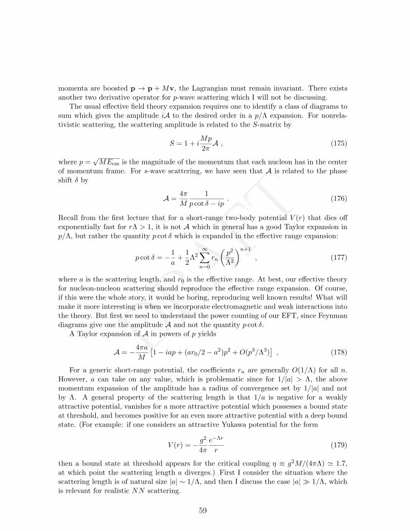
DRAFT

momenta are boosted p → p + Mv, the Lagrangian must remain invariant. There existsanother two derivative operator for p-wave scattering which I will not be discussing.

The usual effective field theory expansion requires one to identify a class of diagrams tosum which gives the amplitude iA to the desired order in a p/Λ expansion. For nonrela-tivistic scattering, the scattering amplitude is related to the S-matrix by

S = 1 + iMp

2πA , (175)

where p =√MEcm is the magnitude of the momentum that each nucleon has in the center

of momentum frame. For s-wave scattering, we have seen that A is related to the phaseshift δ by

A =4π

M

1

p cot δ − ip. (176)

Recall from the first lecture that for a short-range two-body potential V (r) that dies offexponentially fast for rΛ > 1, it is not A which in general has a good Taylor expansion inp/Λ, but rather the quantity p cot δ which is expanded in the effective range expansion:

p cot δ = −1

a+

1

2Λ2

∞∑n=0

rn

(p2

Λ2

)n+1

, (177)

where a is the scattering length, and r0 is the effective range. At best, our effective theoryfor nucleon-nucleon scattering should reproduce the effective range expansion. Of course,if this were the whole story, it would be boring, reproducing well known results! What willmake it more interesting is when we incorporate electromagnetic and weak interactions intothe theory. But first we need to understand the power counting of our EFT, since Feynmandiagrams give one the amplitude A and not the quantity p cot δ.

A Taylor expansion of A in powers of p yields

A = −4πa

M

[1− iap+ (ar0/2− a2)p2 +O(p3/Λ3)

], (178)

For a generic short-range potential, the coefficients rn are generally O(1/Λ) for all n.However, a can take on any value, which is problematic since for 1/|a| > Λ, the abovemomentum expansion of the amplitude has a radius of convergence set by 1/|a| and notby Λ. A general property of the scattering length is that 1/a is negative for a weaklyattractive potential, vanishes for a more attractive potential which possesses a bound stateat threshold, and becomes positive for an even more attractive potential with a deep boundstate. (For example: if one considers an attractive Yukawa potential for the form

V (r) = − g2

4π

e−Λr

r(179)

then a bound state at threshold appears for the critical coupling η ≡ g2M/(4πΛ) ' 1.7,at which point the scattering length a diverges.) First I consider the situation where thescattering length is of natural size |a| ∼ 1/Λ, and then I discuss the case |a| 1/Λ, whichis relevant for realistic NN scattering.

59

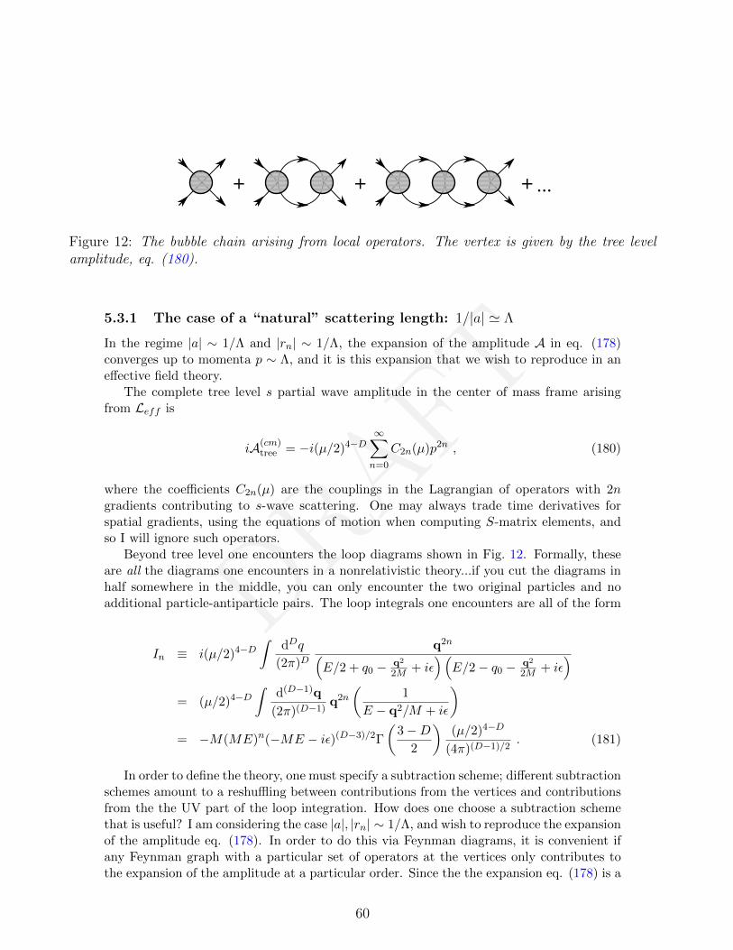
DRAFT

+ +...

+

Figure 12: The bubble chain arising from local operators. The vertex is given by the tree levelamplitude, eq. (180).

5.3.1 The case of a “natural” scattering length: 1/|a| ' Λ

In the regime |a| ∼ 1/Λ and |rn| ∼ 1/Λ, the expansion of the amplitude A in eq. (178)converges up to momenta p ∼ Λ, and it is this expansion that we wish to reproduce in aneffective field theory.

The complete tree level s partial wave amplitude in the center of mass frame arisingfrom Leff is

iA(cm)tree = −i(µ/2)4−D

∞∑n=0

C2n(µ)p2n , (180)

where the coefficients C2n(µ) are the couplings in the Lagrangian of operators with 2ngradients contributing to s-wave scattering. One may always trade time derivatives forspatial gradients, using the equations of motion when computing S-matrix elements, andso I will ignore such operators.

Beyond tree level one encounters the loop diagrams shown in Fig. 12. Formally, theseare all the diagrams one encounters in a nonrelativistic theory...if you cut the diagrams inhalf somewhere in the middle, you can only encounter the two original particles and noadditional particle-antiparticle pairs. The loop integrals one encounters are all of the form

In ≡ i(µ/2)4−D∫

dDq

(2π)Dq2n(

E/2 + q0 − q2

2M + iε)(

E/2− q0 − q2

2M + iε)

= (µ/2)4−D∫

d(D−1)q

(2π)(D−1)q2n

(1

E − q2/M + iε

)= −M(ME)n(−ME − iε)(D−3)/2Γ

(3−D

2

)(µ/2)4−D

(4π)(D−1)/2. (181)

In order to define the theory, one must specify a subtraction scheme; different subtractionschemes amount to a reshuffling between contributions from the vertices and contributionsfrom the the UV part of the loop integration. How does one choose a subtraction schemethat is useful? I am considering the case |a|, |rn| ∼ 1/Λ, and wish to reproduce the expansionof the amplitude eq. (178). In order to do this via Feynman diagrams, it is convenient ifany Feynman graph with a particular set of operators at the vertices only contributes tothe expansion of the amplitude at a particular order. Since the the expansion eq. (178) is a

60

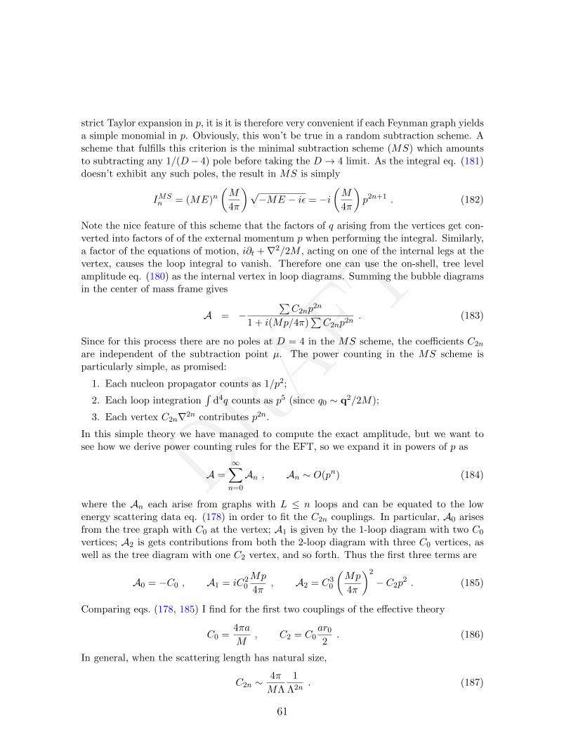
DRAFT

strict Taylor expansion in p, it is it is therefore very convenient if each Feynman graph yieldsa simple monomial in p. Obviously, this won’t be true in a random subtraction scheme. Ascheme that fulfills this criterion is the minimal subtraction scheme (MS) which amountsto subtracting any 1/(D− 4) pole before taking the D → 4 limit. As the integral eq. (181)doesn’t exhibit any such poles, the result in MS is simply

IMSn = (ME)n

(M

4π

)√−ME − iε = −i

(M

4π

)p2n+1 . (182)

Note the nice feature of this scheme that the factors of q arising from the vertices get con-verted into factors of of the external momentum p when performing the integral. Similarly,a factor of the equations of motion, i∂t +∇2/2M , acting on one of the internal legs at thevertex, causes the loop integral to vanish. Therefore one can use the on-shell, tree levelamplitude eq. (180) as the internal vertex in loop diagrams. Summing the bubble diagramsin the center of mass frame gives

A = −∑C2np

2n

1 + i(Mp/4π)∑C2np2n

. (183)

Since for this process there are no poles at D = 4 in the MS scheme, the coefficients C2n

are independent of the subtraction point µ. The power counting in the MS scheme isparticularly simple, as promised:

1. Each nucleon propagator counts as 1/p2;

2. Each loop integration∫

d4q counts as p5 (since q0 ∼ q2/2M);

3. Each vertex C2n∇2n contributes p2n.

In this simple theory we have managed to compute the exact amplitude, but we want tosee how we derive power counting rules for the EFT, so we expand it in powers of p as

A =

∞∑n=0

An , An ∼ O(pn) (184)

where the An each arise from graphs with L ≤ n loops and can be equated to the lowenergy scattering data eq. (178) in order to fit the C2n couplings. In particular, A0 arisesfrom the tree graph with C0 at the vertex; A1 is given by the 1-loop diagram with two C0

vertices; A2 is gets contributions from both the 2-loop diagram with three C0 vertices, aswell as the tree diagram with one C2 vertex, and so forth. Thus the first three terms are

A0 = −C0 , A1 = iC20

Mp

4π, A2 = C3

0

(Mp

4π

)2

− C2p2 . (185)

Comparing eqs. (178, 185) I find for the first two couplings of the effective theory

C0 =4πa

M, C2 = C0

ar0

2. (186)

In general, when the scattering length has natural size,

C2n ∼4π

MΛ

1

Λ2n. (187)

61

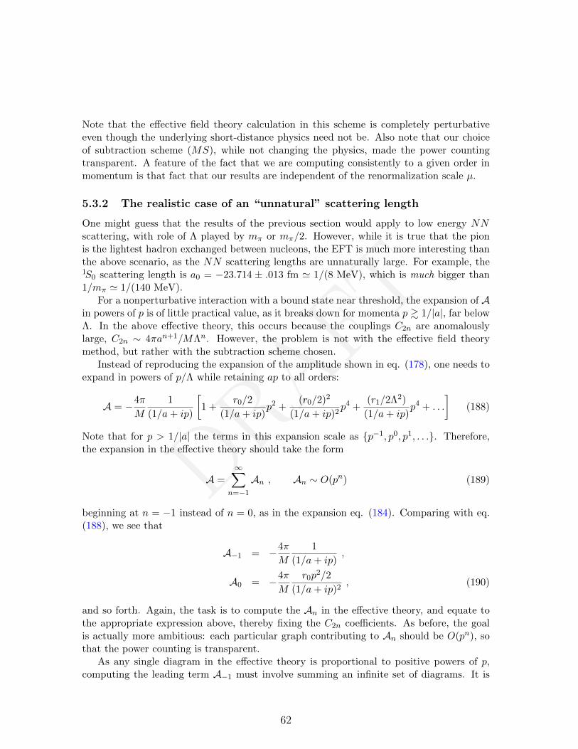
DRAFT

Note that the effective field theory calculation in this scheme is completely perturbativeeven though the underlying short-distance physics need not be. Also note that our choiceof subtraction scheme (MS), while not changing the physics, made the power countingtransparent. A feature of the fact that we are computing consistently to a given order inmomentum is that fact that our results are independent of the renormalization scale µ.

5.3.2 The realistic case of an “unnatural” scattering length

One might guess that the results of the previous section would apply to low energy NNscattering, with role of Λ played by mπ or mπ/2. However, while it is true that the pionis the lightest hadron exchanged between nucleons, the EFT is much more interesting thanthe above scenario, as the NN scattering lengths are unnaturally large. For example, the1S0 scattering length is a0 = −23.714 ± .013 fm ' 1/(8 MeV), which is much bigger than1/mπ ' 1/(140 MeV).

For a nonperturbative interaction with a bound state near threshold, the expansion of Ain powers of p is of little practical value, as it breaks down for momenta p & 1/|a|, far belowΛ. In the above effective theory, this occurs because the couplings C2n are anomalouslylarge, C2n ∼ 4πan+1/MΛn. However, the problem is not with the effective field theorymethod, but rather with the subtraction scheme chosen.

Instead of reproducing the expansion of the amplitude shown in eq. (178), one needs toexpand in powers of p/Λ while retaining ap to all orders:

A = −4π

M

1

(1/a+ ip)

[1 +

r0/2

(1/a+ ip)p2 +

(r0/2)2

(1/a+ ip)2p4 +

(r1/2Λ2)

(1/a+ ip)p4 + . . .

](188)

Note that for p > 1/|a| the terms in this expansion scale as p−1, p0, p1, . . .. Therefore,the expansion in the effective theory should take the form

A =∞∑

n=−1

An , An ∼ O(pn) (189)

beginning at n = −1 instead of n = 0, as in the expansion eq. (184). Comparing with eq.(188), we see that

A−1 = −4π

M

1

(1/a+ ip),

A0 = −4π

M

r0p2/2

(1/a+ ip)2, (190)

and so forth. Again, the task is to compute the An in the effective theory, and equate tothe appropriate expression above, thereby fixing the C2n coefficients. As before, the goalis actually more ambitious: each particular graph contributing to An should be O(pn), sothat the power counting is transparent.

As any single diagram in the effective theory is proportional to positive powers of p,computing the leading term A−1 must involve summing an infinite set of diagrams. It is

62

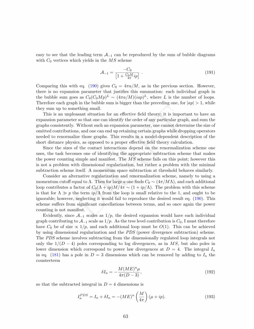
DRAFT

easy to see that the leading term A−1 can be reproduced by the sum of bubble diagramswith C0 vertices which yields in the MS scheme

A−1 =−C0[

1 + C0M4π ip

] . (191)

Comparing this with eq. (190) gives C0 = 4πa/M , as in the previous section. However,there is no expansion parameter that justifies this summation: each individual graph inthe bubble sum goes as C0(C0Mp)L ∼ (4πa/M)(iap)L, where L is the number of loops.Therefore each graph in the bubble sum is bigger than the preceding one, for |ap| > 1, whilethey sum up to something small.

This is an unpleasant situation for an effective field theory; it is important to have anexpansion parameter so that one can identify the order of any particular graph, and sum thegraphs consistently. Without such an expansion parameter, one cannot determine the size ofomitted contributions, and one can end up retaining certain graphs while dropping operatorsneeded to renormalize those graphs. This results in a model-dependent description of theshort distance physics, as opposed to a proper effective field theory calculation.

Since the sizes of the contact interactions depend on the renormalization scheme oneuses, the task becomes one of identifying the appropriate subtraction scheme that makesthe power counting simple and manifest. The MS scheme fails on this point; however thisis not a problem with dimensional regularization, but rather a problem with the minimalsubtraction scheme itself. A momentum space subtraction at threshold behaves similarly.

Consider an alternative regularization and renormalization scheme, namely to using amomentum cutoff equal to Λ. Then for large a one finds C0 ∼ (4π/MΛ), and each additionalloop contributes a factor of C0(Λ + ip)M/4π ∼ (1 + ip/Λ). The problem with this schemeis that for Λ p the term ip/Λ from the loop is small relative to the 1, and ought to beignorable; however, neglecting it would fail to reproduce the desired result eq. (190). Thisscheme suffers from significant cancellations between terms, and so once again the powercounting is not manifest.

Evidently, since A−1 scales as 1/p, the desired expansion would have each individualgraph contributing to A−1 scale as 1/p. As the tree level contribution is C0, I must thereforehave C0 be of size ∝ 1/p, and each additional loop must be O(1). This can be achievedby using dimensional regularization and the PDS (power divergence subtraction) scheme.The PDS scheme involves subtracting from the dimensionally regulated loop integrals notonly the 1/(D − 4) poles corresponding to log divergences, as in MS, but also poles inlower dimension which correspond to power law divergences at D = 4. The integral Inin eq. (181) has a pole in D = 3 dimensions which can be removed by adding to In thecounterterm

δIn = −M(ME)nµ

4π(D − 3), (192)

so that the subtracted integral in D = 4 dimensions is

IPDSn = In + δIn = −(ME)n(M

4π

)(µ+ ip). (193)

63

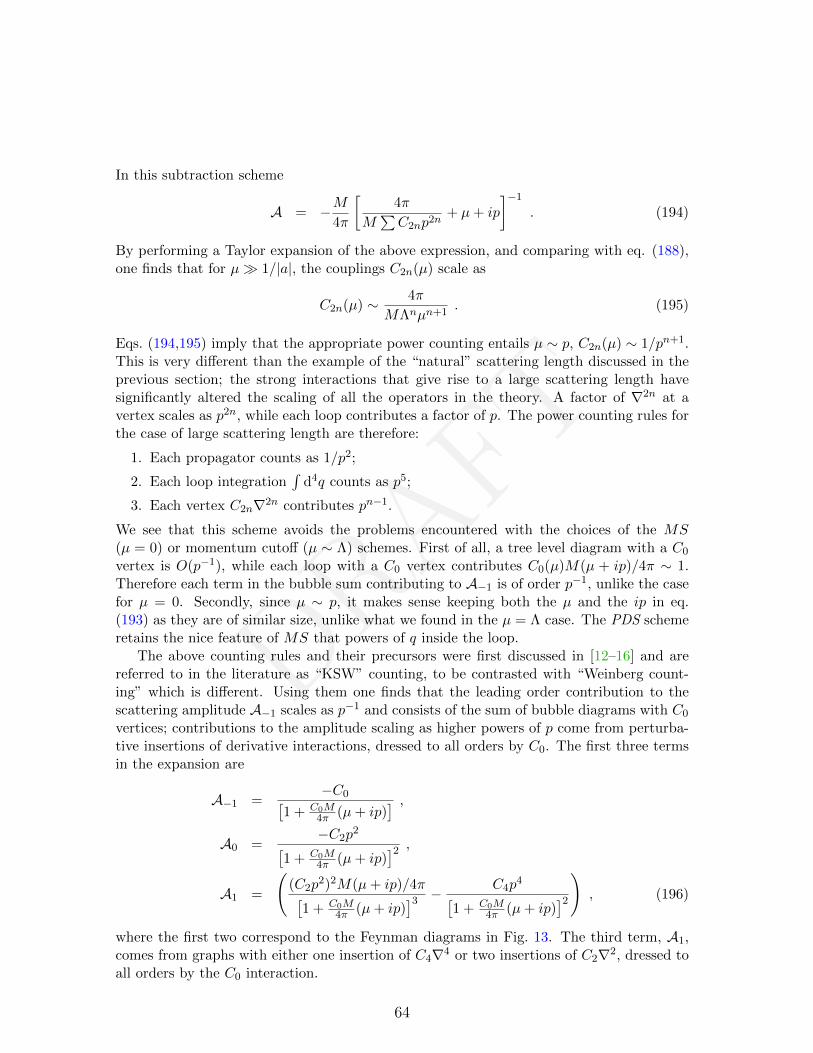
DRAFT

In this subtraction scheme

A = −M4π

[4π

M∑C2np2n

+ µ+ ip

]−1

. (194)

By performing a Taylor expansion of the above expression, and comparing with eq. (188),one finds that for µ 1/|a|, the couplings C2n(µ) scale as

C2n(µ) ∼ 4π

MΛnµn+1. (195)

Eqs. (194,195) imply that the appropriate power counting entails µ ∼ p, C2n(µ) ∼ 1/pn+1.This is very different than the example of the “natural” scattering length discussed in theprevious section; the strong interactions that give rise to a large scattering length havesignificantly altered the scaling of all the operators in the theory. A factor of ∇2n at avertex scales as p2n, while each loop contributes a factor of p. The power counting rules forthe case of large scattering length are therefore:

1. Each propagator counts as 1/p2;

2. Each loop integration∫

d4q counts as p5;

3. Each vertex C2n∇2n contributes pn−1.

We see that this scheme avoids the problems encountered with the choices of the MS(µ = 0) or momentum cutoff (µ ∼ Λ) schemes. First of all, a tree level diagram with a C0

vertex is O(p−1), while each loop with a C0 vertex contributes C0(µ)M(µ + ip)/4π ∼ 1.Therefore each term in the bubble sum contributing to A−1 is of order p−1, unlike the casefor µ = 0. Secondly, since µ ∼ p, it makes sense keeping both the µ and the ip in eq.(193) as they are of similar size, unlike what we found in the µ = Λ case. The PDS schemeretains the nice feature of MS that powers of q inside the loop.

The above counting rules and their precursors were first discussed in [12–16] and arereferred to in the literature as “KSW” counting, to be contrasted with “Weinberg count-ing” which is different. Using them one finds that the leading order contribution to thescattering amplitude A−1 scales as p−1 and consists of the sum of bubble diagrams with C0

vertices; contributions to the amplitude scaling as higher powers of p come from perturba-tive insertions of derivative interactions, dressed to all orders by C0. The first three termsin the expansion are

A−1 =−C0[

1 + C0M4π (µ+ ip)

] ,A0 =

−C2p2[

1 + C0M4π (µ+ ip)

]2 ,

A1 =

((C2p

2)2M(µ+ ip)/4π[1 + C0M

4π (µ+ ip)]3 − C4p

4[1 + C0M

4π (µ+ ip)]2), (196)

where the first two correspond to the Feynman diagrams in Fig. 13. The third term, A1,comes from graphs with either one insertion of C4∇4 or two insertions of C2∇2, dressed toall orders by the C0 interaction.

64

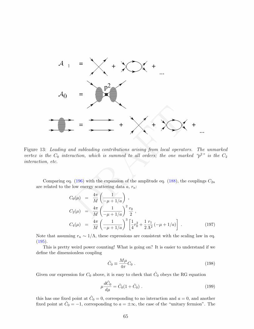
DRAFT

A

1

A

0

=

+

p2

+ +...

=

=

+ +...

Figure 13: Leading and subleading contributions arising from local operators. The unmarkedvertex is the C0 interaction, which is summed to all orders; the one marked “p2” is the C2

interaction, etc.

Comparing eq. (196) with the expansion of the amplitude eq. (188), the couplings C2n

are related to the low energy scattering data a, rn:

C0(µ) =4π

M

(1

−µ+ 1/a

),

C2(µ) =4π

M

(1

−µ+ 1/a

)2 r0

2,

C4(µ) =4π

M

(1

−µ+ 1/a

)3 [1

4r2

0 +1

2

r1

Λ2(−µ+ 1/a)

]. (197)

Note that assuming rn ∼ 1/Λ, these expressions are consistent with the scaling law in eq.(195).

This is pretty weird power counting! What is going on? It is easier to understand if wedefine the dimensionless coupling

C0 ≡Mµ

4πC0 . (198)

Given our expression for C0 above, it is easy to check that C0 obeys the RG equation

µdC0

dµ= C0(1 + C0) . (199)

this has one fixed point at C0 = 0, corresponding to no interaction and a = 0, and anotherfixed point at C0 = −1, corresponding to a = ±∞, the case of the “unitary fermion”. The

65

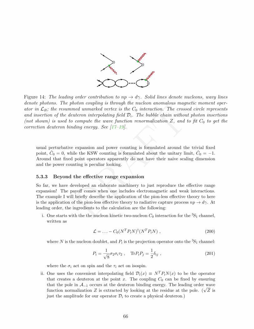
DRAFT

Figure 14: The leading order contribution to np → dγ. Solid lines denote nucleons, wavy linesdenote photons. The photon coupling is through the nucleon anomalous magnetic moment oper-ator in LB; the resummed unmarked vertex is the C0 interaction. The crossed circle representsand insertion of the deuteron interpolating field Di. The bubble chain without photon insertions(not shown) is used to compute the wave function renormalization Z, and to fit C0 to get thecorrection deuteron binding energy. See [17–19].

usual perturbative expansion and power counting is formulated around the trivial fixedpoint, C0 = 0, while the KSW counting is formulated about the unitary limit, C0 = −1.Around that fixed point operators apparently do not have their naive scaling dimensionand the power counting is peculiar looking.

5.3.3 Beyond the effective range expansion

So far, we have developed an elaborate machinery to just reproduce the effective rangeexpansion! The payoff comes when one includes electromagnetic and weak interactions.The example I will briefly describe the application of the pion-less effective theory to hereis the application of the pion-less effective theory to radiative capture process np→ dγ. Atleading order, the ingredients to the calculation are the following:

i. One starts with the the nucleon kinetic two-nucleon C0 interaction for the 3S1 channel,written as

L = . . .− C0(NTPiN)†(NTPiN) , (200)

where N is the nucleon doublet, and Pi is the projection operator onto the 3S1 channel:

Pi =1√8σ2σiτ2 , TrPiPj =

1

2δij , (201)

where the σi act on spin and the τi act on isospin.

ii. One uses the convenient interpolating field Di(x) ≡ NTPiN(x) to be the operatorthat creates a deuteron at the point x. The coupling C0 can be fixed by ensuringthat the pole in A−1 occurs at the deuteron binding energy. The leading order wavefunction normalization Z is extracted by looking at the residue at the pole. (

√Z is

just the amplitude for our operator Di to create a physical deuteron.)

66

DRAFT

iii. np → dγ occurs by emitting a magnetic photon, and so one needs to include in theLagrangian the anomalous magnetic moment interaction of the nucleons:

LB =e

2MNN †(κ0 + κ1τ3)σ ·BN , (202)

where κ0 = 12(κp + κn) and κ1 = 1

2(κp − κn) are the isoscalar and isovector nucleonmagnetic moments with κp = 2.79, κn = −1.91.

iv. Then at leading order one sums up the bubble chain with one insertion of the magneticmoment operator, as shown in Fig. 14.

Figure 15: The graphs contributing to np → dγ at NLO. The black square corresponds to aninsertion of a C2 interaction, the circle to the nucleon anomalous magnetic moment, and theresummed unmarked vertex to the C0 interaction. The last graph is the contribution to wavefunction renormalization at this order. Figure from ref. [19].

From these graphs one finds the capture cross section

σ =8παγ5κ2

1a20

vM5N

(1− 1

γa0

)2

, (203)

where α is the fine structure constant and v is the magnitude of the neutron velocity (in theproton rest frame), a0 = −23.714 ± .013 fm is the 1S0 scattering length and γ ≡

√MNB,

where B is the deuteron binding energy. This agrees with old results of Bethe and Longmirewhen terms in their expression involving the effective range (which are higher order in ourexpansion) are neglected.

At next-to-leading order (“NLO”) one needs to sum all relevant diagrams involving asingle insertion of a C2 vertex (that is, a 2-derivative contact interaction, whose value is fit

67

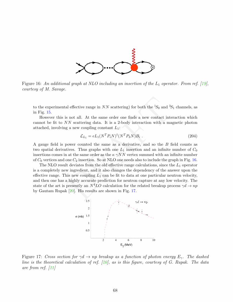
DRAFT

Figure 16: An additional graph at NLO including an insertion of the L1 operator. From ref. [19],courtesy of M. Savage.

to the experimental effective range in NN scattering) for both the 1S0 and 3S1 channels, asin Fig. 15.

However this is not all. At the same order one finds a new contact interaction whichcannot be fit to NN scattering data. It is a 2-body interaction with a magnetic photonattached, involving a new coupling constant L1:

LL1 = eL1(NTPiN)†(NTP3N)Bi . (204)

A gauge field is power counted the same as a derivative, and so the B field counts astwo spatial derivatives. Thus graphs with one L1 insertion and an infinite number of C0

insertions comes in at the same order as the κ γNN vertex summed with an infinite numberof C0 vertices and one C2 insertion. So at NLO one needs also to include the graph in Fig. 16.

The NLO result deviates from the old effective range calculations, since the L1 operatoris a completely new ingredient, and it also changes the dependency of the answer upon theeffective range. This new coupling L1 can be fit to data at one particular neutron velocity,and then one has a highly accurate prediction for neutron capture at any low velocity. Thestate of the art is presently an N4LO calculation for the related breakup process γd→ npby Gautam Rupak [20]. His results are shown in Fig. 17.

2 4 6 8 10

0.5

1

1.5

2

2.5

Eγ (MeV)

σ (mb)

d! np

Figure 17: Cross section for γd → np breakup as a function of photon energy Eγ. The dashedline is the theoretical calculation of ref. [20], as is this figure, courtesy of G. Rupak. The dataare from ref. [21]

68

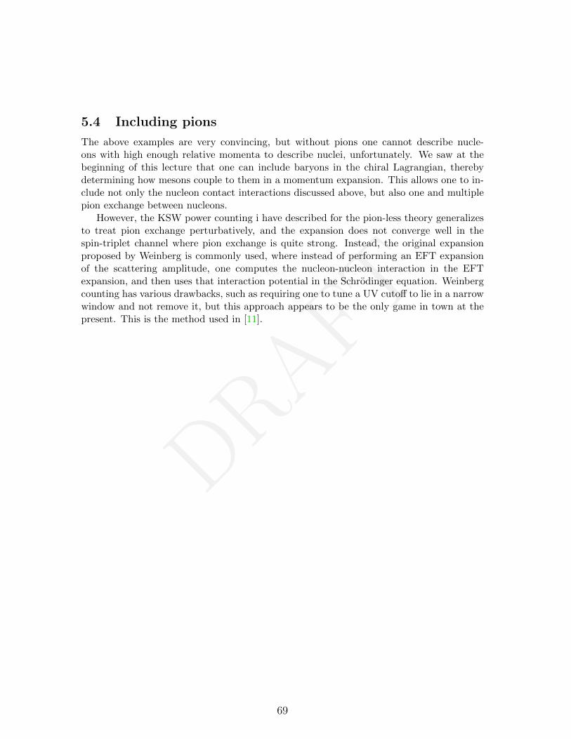
DRAFT

5.4 Including pions

The above examples are very convincing, but without pions one cannot describe nucle-ons with high enough relative momenta to describe nuclei, unfortunately. We saw at thebeginning of this lecture that one can include baryons in the chiral Lagrangian, therebydetermining how mesons couple to them in a momentum expansion. This allows one to in-clude not only the nucleon contact interactions discussed above, but also one and multiplepion exchange between nucleons.

However, the KSW power counting i have described for the pion-less theory generalizesto treat pion exchange perturbatively, and the expansion does not converge well in thespin-triplet channel where pion exchange is quite strong. Instead, the original expansionproposed by Weinberg is commonly used, where instead of performing an EFT expansionof the scattering amplitude, one computes the nucleon-nucleon interaction in the EFTexpansion, and then uses that interaction potential in the Schrodinger equation. Weinbergcounting has various drawbacks, such as requiring one to tune a UV cutoff to lie in a narrowwindow and not remove it, but this approach appears to be the only game in town at thepresent. This is the method used in [11].

69

DRAFT

6 Chiral lagrangians for BSM physics

6.1 Technicolor

Chiral lagrangians are the tool for studying the physics of Goldstone bosons. The pionsin particular are the ones we have been looking at, but we know that there are at leastthree other Goldstone bosons in reality: namely the three that are “eaten” via the Higgsmechanism and become the longitudinal degrees of freedom in the W± and the Z0 gaugebosons in the SM. Let us start by asking what the world would look like if the Higgs doubletwas omitted from the SM; to make this toy model simpler, let’s also imagine that the worldonly has one family of fermions, u, d, e, νe, and in the following discussion I will ignore theleptons.

Without the Higgs the SU(2) × U(1) gauge bosons are all massless down at the QCDscale and have to be included in the chiral Lagrangian. Therefore we need only consider anSU(2)× SU(2)/SU(2) chiral Lagrangian, where the Σ field represents the three pions andis written as

Σ = e2iTaπa/fπ , Ta =σa2, (205)

but how do we incorporate the gauge fields? Recall that in the SM the gauge charges ofthe quarks under SU(2)× U(1) are(

ud

)L

= 2 16, uR = 1 2

3, dR = 1− 1

3. (206)

Note that the SU(2)L of the chiral Lagrangian is exactly the same group as the SU(2)Lthat is gauged in the SM; the gauged U(1) charge Y can be written as

Y =1

2B + T3,R (207)

where B is baryon number, the U(1)V symmetry that acts the same on all LH and RHquarks, and T3,R ∈ SU(2)R. The U(1)V part is uninteresting in the chiral Lagrangian sincethe pions do not carry that quantum number; however we have to use covariant derivativesfor the SU(2)L × U(1)R part of the gauge group:

∂µΣ =⇒ DµΣ = ∂µΣ + igW aµTaΣ− ig′BµΣT3 , (208)

where I used the fact that under SU(2)× SU(2) the Σ field transforms as Σ→ LΣR†; thedagger on R is what is responsible for the minus sign in front of the U(1) gauge boson pieceabove.

Something peculiar is going on: now that SU(2)L is gauged, the matrix L is promotedto a spacetime dependent matrix L(x), and I can choose L(x) = Σ†(x)...and a gaugetransformation can turn Σ into the unit matrix! This is because the quark condensate〈qLqR〉 has broken the weak interactions spontaneously, the W and B get masses, and wejust rediscovered unitary gauge.

Now let’s look at the kinetic term for the Σ field in unitary gauge:

f2

4TrDµΣ(DµΣ)† =

f2

4

[g2W a

µWµbTrTaTb − 2gg′W 3

µBµTrT3T3 + g′2TrT3T3

]. (209)

70

DRAFT

This gives us a mass2 matrix for the gauge bosons

M2 =f2

4

g2

g2

g2 −gg′−gg′ g′2

(210)

with eigenvalues

m2 =

0,

g2f2

4,g2f2

4,

(g2 + g′2)f2

4

≡m2γ , m

2w, m

2w, mz

2

(211)

where

m2γ = 0 , m2

w =e2f2

π

4 sin2 θw, m2

z =m2w

cos2 θw(212)

with the conventional definitions g = e/ sin θw, g′ = e/ cos θw.This would look precisely like the SM if instead of fπ = 93 MeV we took fπ = 250 GeV!

This was the observation of both Weinberg and Susskind [22–24]: that the strong inter-actions would provide the Higgs mechanism in the SM without the Higgs doublet field.While the W and Z would get massive, as in the SM, in this theory there might not be anactual Higgs boson (it is not in the chiral Lagrangian, and QCD does not have any narrow0+ resonance), and the order parameter for the symmetry breaking is a quark bilinear nowinstead of a fundamental scalar, and so that there is no naturalness problem: the weak scaleis set by the QCD scale, which can be naturally much smaller than the GUT or Planckscales due to asymptotic freedom, just as Cooper pairs in superconductivity are so muchlarger than the crystal lattice spacing.

However, fπ 6= 250 GeV and we do not want to give away the pion. So instead weposit a new gauge interaction, just like color but at a higher scale called technicolor, andnew fermions that carry this gauge quantum number, U , D, called techniquarks. Nowthe techniquarks condense with a technipion decay constant FΠ = 250 GeV, and we haveexplained the SM without the Higgs!

This is great, except for three problems: (i) the Higgs boson has been discovered, longafter the invention of technicolor, while there is no analogously light 0+ meson in the stronginteractions; (ii) it is difficult to construct a technicolor theory where precision radiativecorrections to the weak interactions agree with what is measured; (iii) as described here, thetechniquark condensate only fulfills one of the roles played by the Higgs serves in the SM:giver of mass to the gauge bosons. To realize the other role — giver of mass to the quarks andleptons — requires new interactions added to be technicolor (e.g., Extended Technicolor),more complications, and serious problems with flavor changing neutral currents. There aremore complex versions of the original theory still being explored, but the compelling beautyof the original concept is no longer there.

6.2 Composite Higgs

What is so beautiful about technicolor is that by replacing the fundamental Higgs scalar fieldwith a quark bilinear, the fine tuning problem is avoided. Do we have to abandon that idea

71

DRAFT

simply because we have seen a Higgs boson that looks fundamental? No, that has happenedbefore: the pions looked fundamental when discovered, and only over a decade later was itdecided that they were composite bound states. Furthermore, they are relativistic boundstates – at least in the chiral limit, their compositeness scale is much smaller than theirCompton wavelengths. Relativistic bound states are in general baffling things we have nohandle on as they always require strong coupling. One of the few exceptions when weunderstand what is going on exception is when the bound states are Goldstone bosons, likethe pions in QCD. So let us return to the QCD chiral Lagrangian for inspiration, this timenot looking at the pions as candidates for the longitudinal W and Z, but at the kaons ascandidates for the Higgs doublet [25,26].

A Higgs doublet field has four real degrees of freedom, so we need to look at a chiral La-grangian with at least four Goldstone bosons. The SU(2)×SU(2)/SU(2) chiral Lagrangianonly has three pions, so that won’t do; however the SU(3) × SU(3)/SU(3) example haseight mesons. Furthermore, there is a ready made SU(2) doublet in that theory – the kaon.In fact, note that under the unbroken isospin and strong hypercharge SU(2)×U(1) globalsymmetry of QCD, the kaon doublet transforms just like the Higgs doublet does undergauged electroweak SU(2)× U(1) symmetry in the SM. So what if we scaled up a versionof QCD with three massless flavors, gauge the vector-like SU(2) × U(1) symmetry, andidentify the kaon doublet with the Higgs doublet?

In such a theory the Higgs would get a mass from SU(2) × U(1) gauge interactions,just as the π+ gets a mass contribution from electromagnetic contributions (see problem6). Unfortunately this contribution to the Higgs mass2 is positive, and so there is nospontaneous symmetry breaking in the model so far. What is needed is some effect thatcontributes a negative mass2. Various examples have been found that will do this: one isan axial gauge group under which the constituents of the composite Higgs are charged [27];another and more compelling source of destabilization of the composite Higgs potential isthe top quark [2]. The basic idea is that operators can be induced in the chiral Lagrangianwhich favor the vacuum Σ 6= 1 and prefer a small nonzero value corresponding to thecomposite Higgs doublet getting a vev v which can be computable in terms of f and couplingconstants, such as the top Yukawa coupling. The example of vacuum destabilization froman axial gauge interaction is easy to understand. We have seen in eq. (4.3.2) that theoperator which gives the positive electromagnetic contribution to the π+ and K+ mass2 is:

Lα = ξf4 α

4πTrQLΣQRΣ† = ξ

α

6πf4 − 2ξ

α

9πf2(π+π− +K+K−

)+ . . . (213)

where QR = QL = diag2/3,−1/3,−1/3. If we had gauged an “axial electromagnetic”U(1) symmetry instead with QR = −QL, then this contribution to the kaon mass2 wouldbe m2

K+ = −2ξ α9πf2 — and if there were no quark masses, this would be the leading

contribution and would signal that the vacuum with 〈K〉 = 0 is unstable. A vev for thekaon implies a vev for Σ which is not the unit matrix: the quark condensate misaligns fromthe SU(2)× U(1) symmetry preserving direction, breaking the weak interactions. If thereare competing positive and negative contributions to the kaon mass2 it is possible to selectwhatever value one wants for v/f , and if v/f 1, then the composite Higgs will lookvery much like the SM Higgs – one will need to probe energies on the order of f to see itscomposite nature.

72

DRAFT

This scale v is set to 250 GeV and is the usual Higgs vev; the theory then predicts ata higher scale Λ ' 4πf the Higgs will reveal itself to be composite. The smaller the ratiov/f , the more fundamental the Higgs will appear at low energy. For a recent discussion ofthe viability of the composite Higgs idea and accelerator tests, see [28].

6.2.1 The axion

A problem that afflicts QCD is that one can add to the action the operator

−θ g2

16π2TrGµνGµν (214)

and even though it is a total derivative, the topology of the vacuum allows it to have aphysical effect. Because of the Levi-Civita symbol in the definition of Gµν , this operatorviolates P and T , while conserving C. Thus it is CP violating, and it can contribute to CP -violating observables in hadrons, such as the neutron electric dipole moment. Experimentalbounds on the neutron EDM imply that θ . 10−9. This fine tuning is called the strongCP problem. If we consider the vacuum energy E(θ) as a function of θ it is intriguing thatits minimum is at θ = 0 [29]. However θ is like a coupling constant and cannot change itsvalue to minimize the energy. The brilliant observation by Peccei and Quinn [30] was thatit is possible to construct a theory where θ gets replaced by a dynamical field which canrelax to zero; this field gives rise to a light particle [31,32] called the axion.

It was discovered in the late 1960s and early 1970s that classical symmetries can bebroken by quantum effects involving gauge fields, called anomalies. Furthermore, if thatsymmetry is spontaneously broken and the gauge fields are not strongly interacting, theresultant pseudo Goldstone boson will couple to gauge fields very much like the θ parameterabove. For example, the linear combination of SU(3)L×SU(3)R currents qγµγ5T

3q has anelectromagnetic anomaly since TrT 3Q2 6= 0, and it is spontaneously broken by the quarkcondensate as well, giving rise to the π0 pseudo Goldstone boson, which as a consequenceof the anomaly, has a coupling to photons of the form

α

4π

π0

fπFF (215)

So the Peccei Quinn mechanism involves introducing a global symmetry that has a coloranomaly and which is spontaneously broken at high energy; this will result in a pseudoGoldstone boson coupling like θ. For example, consider adding a Dirac color-triplet quarkQ to the standard model which is neutral under the weak interactions, and add a complexscalar field Φ with the Lagrangian

L = Qi /DQ+ |∂Φ|2 − V (|Φ|2)− yQLΦQR + h.c. , (216)

where Dµ is the SU(3) covariant derivative. This Lagrangian has a global symmetry

Q → eiωγ5Q , Φ→ e−2iωΦ , (217)

which has a color anomaly. If the scalar potential breaks this symmetry with 〈Φ〉 = fa/√

2,where fa ΛQCD has dimension of mass, then the exotic quark Q gets very heavy with

73

DRAFT

mass yfa/√

2 and the only light mode that survives is a pseudo Goldstone boson a(x), theaxion, which couples to glue via the anomaly:

Left = −a(x)

fa

g2

16π2TrGµνGµν (218)

So we see that θ is replaced with the dynamical quantity a(x)/fa. If there was a nonzero θin the orginal theory, we have shifted the axion field to absorb it. Now the question is, is〈a〉 = 0?

How do we figure out how the axion couples to matter? In general we do not knowhow to analytically compute the effect of gluon operators, but in the present case we can.Consider QCD with the u, d, s quarks included in the theory:

L = qi /Dq − qRMqL + h.c.− a(x)

fa

g2

16π2TrGµνGµν , q =

uds

. (219)

If we perform a spacetime dependent axial rotation on the quarks

q → e−iβ(x)Qaxγ5q (220)

where Qax is some diagonal 3× 3 matrix to be determined, then in terms of the new fieldsthe theory is

L = qi /Dq − i∂µβγµγfQaxq − qRMe2iβ(x)QaxqL + h.c.

−[a(x)

fa− β(x)TrQax

]g2

16π2TrGµνGµν +

α

2πβ(x)(3TrQaxQ

2)FF . (221)

where the shift in the GG (FF ) is due to the color (electromagnetic) anomaly of thetransformation, which for the color anomaly is proportional to TrQaxTaTb = 1

2δabTrQax,where the Ta are color generators, with the analogous expression with Ta,b replaced by theelectric charge matrix for the electromagnetic anomaly, and a factor of three for color. Soif we choose

TrQax = 1 , β(x) = a(x)/(fa) , (222)

we can remove the GG coupling entirely and obtain

L = qi /Dq − i∂µa2fa

qγµγ5Qaxq − qRMei2a(x)Qax/faqL + h.c. +α

2π

a

faTrQaxQ

2 FF

(223)

We know how to match this Lagrangian onto the chiral Lagrangian because (i) the derivativecouplings of the axion match onto symmetry currents in the chiral Lagrangian; (ii) the masscoupling just involves replacing the quark mass matrix M →Me2ia(x)Qax/fa everywhere inour previous analysis; (iii) the electormagnetic coupling of the axion is the same in thechiral Lagrangian, not involving any strong interactions.

Note that we have not fixed Qax yet, beyond requiring TrQax = 1. We will do so shortly.

74

DRAFT

I will ignore the derivative and electromagnetic couplings of the axion and focus on itspotential, arising from the mass term. By modifying eq. (122) we now have in the chiralLagrangian the term

LM =1

2f2πΛTrMei2a(x)Qax/faΣ + h.c.

=1

2f2πΛTrM

[(1 + 2iaQax/fa − 2a2Q2

ax/f2a + . . .)(1 + 2iπ/fπ − 2π2/f2

π + . . .)]

+ h.c.

(224)

Note that the terms linear in either a or π vanish because of the “+h.c.”. However, ingeneral there will be a mass mixing term between the meson and the axion field (moreprecisely, between a, π0 and η). We can eliminate this term from the start by choosing

Qax =M−1

TrM−1=

1

mumd +mdms +msmu

mdms

msmu

mumd

=

1

mu +md

md

mu

0

+O

(mu

ms

)+O

(md

ms

). (225)

Note that this has unit trace as we required; it also eliminates the mixing term by cancellingoff the factor of M in the trace, since Trπ = 0. With this choice for Qax we can now easilycompute the axion mass and find

LM = −2a2 f2πΛ

f2a

TrMQ2ax + . . . = −1

2a2 4f2

πΛ

f2aTrM−1

(226)

If we use our previous result m2π = Λ(mu +md) we can read off the axion mass as

m2a =

4f2πΛ

f2aTrM−1

' f2πm

2π

f2a

(4mumd

(mu +md)2

)(227)

where I have dropped terms proportional to 1/ms in the expression on the right. Withmu/md ' 1/2, the factor on the right is very close to 1/4. Note that the axion mass scalesas our undetermined parameter 1/fa. You can easily show that the axion is odd under CP ,and since a positive mass2 for the axion implies the minimum of the axion potential is at〈a〉 = 0, and since we have no θ parameter, the strong interactions are now CP conservingas observed in nature.

If we ignore isospin breaking and set mu = md, then we get the full axion potential verysimply,

V (a) = −m2af

2a cos

a

fa= −m2

πf2π cos

a

fa(228)

The axion model is beautiful, and really is the only known soltuion to the strong CPproblem that is viable. Now the ugly facts about the model: it is critical that the entireaxion potential come from QCD so that the minimum is at 〈a〉 = 0. This is equivalent to say

75

DRAFT

that the only operator in the theory that does not respect the global PQ symmetry is thegluon anomaly term, eq. (218). However, it is believed that quantum gravity violates globalcharges: if you through global charge into a black hole, it is lost. So one might expect highdimension operators that violate the PQ symmetry, suppressed by the appropriate powersof the Planck mass Mp, such as cΦ6/M2

p + h.c.. However, this will typically favor a nonzerovev for the axion. It turns out one must forbid such operators up to dimension ten or so, forno obvious good reason, to ensure that the PQ mechanism solves the strong CP problem.

6.2.2 Axion cosmology and the anthropic axion

The axion potential vanishes at high temperature (compared to ΛQCD because (i) chiralsymmetry is restored, and (ii) instantons become rapidly unimportant at high temperature,in which case the GG term is unimportant. The Peccei-Quinn (PQ) symmetry breakingscale fa is high compared to ΛQCD and therefore when Φ gets a vev, it sees a completelydegenerate choice of minima, meaning a vanishing potential for the axion. Thus 〈a/fa〉will select some random value in the early universe, but at T ∼ ΛQCD will find it is not atthe minimum of its potential, and when its Compton wavelength comes within the horizon,it will start oscillating, and there will be a lot of energy in the field. If it is spatiallyuniform and oscillating in time, it looks like a Bose-Einstein condensate of axions at rest,and will dilute as R9t0−3, where R(t) is the cosmic scale factor, like any nonrelativisticmatter. Because of the weak couplings to ordinary matter, suppressed by 1/fa, the axionswill not thermalize and become relativistic. When one computes the relic energy in theaxions today, on finds that it increases with fa, and that axions could be the dark matterif fa ∼ 1012 GeV; if fa is larger, then too large a fraction of the mass budget is in darkmatter.

One might think that if the axion just happened to be close to the right minimum fromthe start, then the dark matter that results could be made small for any fa. However, ifPQ symmetry breaking occurs below the reheat temperature after inflation, today’s horizonresults from many causally disconnected horizons at the PQ symmetry breaking scale, andit would violate causality to force a/fa to have initial values near zero over all of theseregions.

If the PQ symmetry breaks before inflation, then the initial horizon gets stretch overa volume much larger than today’s horizon, and it is possible for the axion to have anaccidentally small initial value, allowing large fa without problem. It seems that we havesubstituted one fining problem (why θ is small) with a similar one (why the initial valuefor 〈a/fa〉 is small in the patch that becomes our horizon). However here one can actuallymake a convincing anthropic argument:

• We know that all possible values of a/fa will occur below the PQ scale for 0 ≤ a/fa ≤2π with equal probability;

• We know how to compute the dark matter abundance today in an axion model; unlessthe initial value of a/fa is very close to zero, most of Ω today will come from darkmatter;

• In a heavily dark matter dominated universe, black holes are created instead of galax-ies, and life is impossible;

76

DRAFT

• Therefore while patches of the universe with Ωdm not very close to unity are very rare,life only can exist in such patches, which is why we think the initial condition for theaxion was fine-tuned.

In my mind, this is the only solid anthropic argument particle physicists know how tomake; see [33]. This example does not really have anything to do with the fine tuningissues associated with irrelevant operators, but since less solid anthropic arguments havebeen made to explain the cosmological constant and the Higgs mass, I thought I wouldshow you this example of anthropic reasoning. It is the most solid example I know becauseit is the only example where we have a thorough understanding of the ab initio probabilitydistribution for some fundamental parameter, since we have a complete dynamical modelfor how the axion comes about.

6.2.3 The Relaxion

A very clever dynamical explanation for why the Higgs is light, sort of along the lines of theparable of the previous lecture, is the relaxion model of [6]. I like this example because itshows one possible way out from the fine tuning problem associated with a relevant operator– the Achilles heel of the EFT approach to quantum field theory – in this case the Higgsmass term.

The basic idea is to take the axion and very weakly break the PQ symmetry explicitlyby coupling it to the Higgs. For the Higgs-axion sector we take the Lagrangian

L = (−M2 + gφ)|h|2 − V (gφ)− αs16π2

φ

fTrGG , (229)

where h is the Higgs, φ is the axion, and g is the small symmetry breaking parameter withdimension of mass; the mass M is taken to be the cutoff in the theory (very large comparedto the weak scale). The potential V is assumed to be a function only of gφ,with dimensionsmade up by powers of the cutoff M :

V ∼M2gφ+ g2φ2 +g3φ3

M2+ . . . (230)

You should check that this is not an unnatural potential: none of the terms are smallcompared to their radiative corrections. This theory does not solve the strong CP problemany more, and the cosmology is somewhat problematic, but it has an very interestingpotential for the axion. Suppose the initial value for φ is large and negative. Then theHiggs has a large positive mass, gets integrated out of the theory, and the quarks in theSM are massless. In this case the pion is massless and the QCD generated potential forthe axion eq. (228) vanishes. So the axion sees the −M2gφ term in its potential and startsrolling toward positive values. As it does so, it makes the Higgs lighter, and eventually itreaches the point where the Higgs mass2 goes negative and the Higgs gets a vev. At thispoint the pion becomes massive and the potential eq. (228) turns on, adding ripples to thepotential. If it keeps rolling, then the Higgs vev keeps getting bigger, making the potentialwiggles bigger. Eventually the axion hits a barrier it can’t get over and stops, a pointwhere the M2gφ term balances against the m2

πf2π/f

2 cosφ/f potential. With appropriatelychosen parameters, this can naturally be at a Higgs vev 〈h〉 M .

77

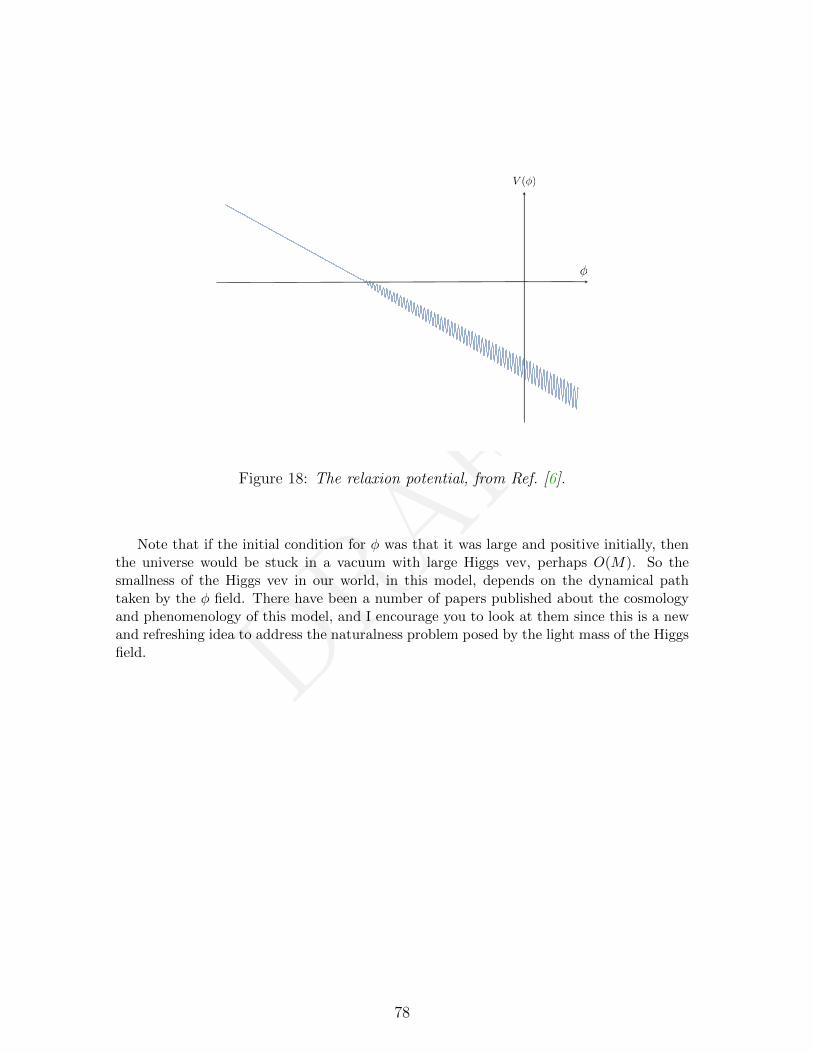
DRAFT

V ()

Figure 18: The relaxion potential, from Ref. [6].

Note that if the initial condition for φ was that it was large and positive initially, thenthe universe would be stuck in a vacuum with large Higgs vev, perhaps O(M). So thesmallness of the Higgs vev in our world, in this model, depends on the dynamical pathtaken by the φ field. There have been a number of papers published about the cosmologyand phenomenology of this model, and I encourage you to look at them since this is a newand refreshing idea to address the naturalness problem posed by the light mass of the Higgsfield.

78

DRAFT

References

[1] D. B. Kaplan, Flavor at SSC energies: A New mechanism for dynamically generatedfermion masses, Nucl.Phys. B365 (1991) 259–278.

[2] K. Agashe, R. Contino, and A. Pomarol, The Minimal composite Higgs model,Nucl.Phys. B719 (2005) 165–187, [hep-ph/0412089].

[3] H. Georgi, H. R. Quinn, and S. Weinberg, Hierarchy of Interactions in Unified GaugeTheories, Phys.Rev.Lett. 33 (1974) 451–454.

[4] S. Weinberg, Anthropic Bound on the Cosmological Constant, Phys.Rev.Lett. 59(1987) 2607.

[5] D. B. Kaplan and A. E. Nelson, Inflationary Axion Cosmology Beyond Our Horizon,arXiv:0809.1206.

[6] P. W. Graham, D. E. Kaplan, and S. Rajendran, Cosmological Relaxation of theElectroweak Scale, Phys. Rev. Lett. 115 (2015), no. 22 221801, [arXiv:1504.07551].

[7] J. Polchinski, Effective Field Theory and the Fermi Surface, hep-th/9210046.

[8] T. Schaefer, Quark Matter, hep-ph/0304281.

[9] S. Weinberg, Nuclear Forces from Chiral Lagrangians, Phys.Lett. B251 (1990)288–292.

[10] S. Weinberg, Effective Chiral Lagrangians for Nucleon - Pion Interactions andNuclear Forces, Nucl.Phys. B363 (1991) 3–18.

[11] E. Epelbaum, H.-W. Hammer, and U.-G. Meissner, Modern Theory of NuclearForces, Rev. Mod. Phys. 81 (2009) 1773–1825, [arXiv:0811.1338].

[12] U. van Kolck, Nucleon-nucleon interaction and isospin violation, hep-ph/9711222.[Lect. Notes Phys.513,62(1998)].

[13] P. F. Bedaque and U. van Kolck, Nucleon Deuteron Scattering from an EffectiveField Theory, Phys.Lett. B428 (1998) 221–226, [nucl-th/9710073].

[14] U. van Kolck, Effective field theory of short range forces, Nucl. Phys. A645 (1999)273–302, [nucl-th/9808007].

[15] D. B. Kaplan, M. J. Savage, and M. B. Wise, A New Expansion for Nucleon-NucleonInteractions, Phys.Lett. B424 (1998) 390–396, [nucl-th/9801034].

[16] D. B. Kaplan, M. J. Savage, and M. B. Wise, Two Nucleon Systems from EffectiveField Theory, Nucl.Phys. B534 (1998) 329–355, [nucl-th/9802075].

[17] D. B. Kaplan, M. J. Savage, and M. B. Wise, A Perturbative Calculation of theElectromagnetic Form-Factors of the Deuteron, Phys.Rev. C59 (1999) 617–629,[nucl-th/9804032].

[18] D. B. Kaplan, M. J. Savage, R. P. Springer, and M. B. Wise, An effective field theorycalculation of the parity violating asymmetry in polarized np→ dγ, Phys.Lett. B449(1999) 1–5, [nucl-th/9807081].

[19] J.-W. Chen, G. Rupak, and M. J. Savage, Nucleon-Nucleon Effective Field Theorywithout Pions, Nucl.Phys. A653 (1999) 386–412, [nucl-th/9902056].

79

DRAFT

[20] G. Rupak, Precision Calculation of N P —&Gt; D Gamma Cross-Section for BigBang Nucleosynthesis, Nucl.Phys. A678 (2000) 405–423, [nucl-th/9911018].

[21] H. Arenhovel and M. Sanzone, Photodisintegration of the deuteron: A review oftheory and experiment, . Springer-Verlag (1991).

[22] S. Weinberg, Implications of Dynamical Symmetry Breaking, Phys.Rev. D13 (1976)974–996.

[23] S. Weinberg, Implications of Dynamical Symmetry Breaking: An Addendum,Phys.Rev. D19 (1979) 1277–1280.

[24] L. Susskind, Dynamics of Spontaneous Symmetry Breaking in the Weinberg-SalamTheory, Phys.Rev. D20 (1979) 2619–2625.

[25] D. B. Kaplan and H. Georgi, SU(2) × U(1) Breaking by Vacuum Misalignment,Phys.Lett. B136 (1984) 183.

[26] M. J. Dugan, H. Georgi, and D. B. Kaplan, Anatomy of a Composite Higgs Model,Nucl.Phys. B254 (1985) 299.

[27] T. Banks, CONSTRAINTS ON SU(2) x U(1) BREAKING BY VACUUMMISALIGNMENT, Nucl.Phys. B243 (1984) 125.

[28] R. Contino, C. Grojean, D. Pappadopulo, R. Rattazzi, and A. Thamm, Strong HiggsInteractions at a Linear Collider, JHEP 1402 (2014) 006, [arXiv:1309.7038].

[29] C. Vafa and E. Witten, Parity Conservation in QCD, Phys. Rev. Lett. 53 (1984) 535.

[30] R. D. Peccei and H. R. Quinn, Constraints Imposed by CP Conservation in thePresence of Instantons, Phys. Rev. D16 (1977) 1791–1797.

[31] S. Weinberg, A New Light Boson?, Phys. Rev. Lett. 40 (1978) 223–226.

[32] F. Wilczek, Problem of Strong p and t Invariance in the Presence of Instantons,Phys. Rev. Lett. 40 (1978) 279–282.

[33] M. Tegmark, A. Aguirre, M. Rees, and F. Wilczek, Dimensionless constants,cosmology and other dark matters, Phys. Rev. D73 (2006) 023505,[astro-ph/0511774].

80