lectures on risk theory
TRANSCRIPT
Lectures on Risk Theory
Klaus D. Schmidt
Lehrstuhl fur VersicherungsmathematikTechnische Universitat Dresden
December 28, 1995
To the memory of
Peter Hess
and
Horand Stormer

Preface
Twenty–five years ago, Hans Buhlmann published his famous monograph Mathe-matical Methods in Risk Theory in the series Grundlehren der MathematischenWissenschaften and thus established nonlife actuarial mathematics as a recognizedsubject of probability theory and statistics with a glance towards economics. Thisbook was my guide to the subject when I gave my first course on nonlife actuarialmathematics in Summer 1988, but at the same time I tried to incorporate into mylectures parts of the rapidly growing literature in this area which to a large extentwas inspired by Buhlmann’s book.
The present book is entirely devoted to a single topic of risk theory: Its subject isthe development in time of a fixed portfolio of risks. The book thus concentrates onthe claim number process and its relatives, the claim arrival process, the aggregateclaims process, the risk process, and the reserve process. Particular emphasis islaid on characterizations of various classes of claim number processes, which providealternative criteria for model selection, and on their relation to the trinity of thebinomial, Poisson, and negativebinomial distributions. Special attention is also paidto the mixed Poisson process, which is a useful model in many applications, to theproblems of thinning, decomposition, and superposition of risk processes, which areimportant with regard to reinsurance, and to the role of martingales, which occurin a natural way in canonical situations. Of course, there is no risk theory withoutruin theory, but ruin theory is only a marginal subject in this book.
The book is based on lectures held at Technische Hochschule Darmstadt and later atTechnische Universitat Dresden. In order to raise interest in actuarial mathematicsat an early stage, these lectures were designed for students having a solid backgroundin measure and integration theory and in probability theory, but advanced topics likestochastic processes were not required as a prerequisite. As a result, the book startsfrom first principles and develops the basic theory of risk processes in a systematicmanner and with proofs given in great detail. It is hoped that the reader reachingthe end will have acquired some insight and technical competence which are usefulalso in other topics of risk theory and, more generally, in other areas of appliedprobability theory.
I am deeply indebted to Jurgen Lehn for provoking my interest in actuarial mathe-matics at a time when vector measures rather than probability measures were on my
viii Preface
mind. During the preparation of the book, I benefitted a lot from critical remarksand suggestions from students, colleagues, and friends, and I would like to expressmy gratitude to Peter Amrhein, Lutz Kusters, and Gerd Waldschaks (UniversitatMannheim) and to Tobias Franke, Klaus–Thomas Heß, Wolfgang Macht, BeatriceMensch, Lothar Partzsch, and Anja Voss (Technische Universitat Dresden) for thevarious discussions we had. I am equally grateful to Norbert Schmitz for severalcomments which helped to improve the exposition.
Last, but not least, I would like to thank the editors and the publishers for acceptingthese Lectures on Risk Theory in the series Skripten zur Mathematischen Stochastikand for their patience, knowing that an author’s estimate of the time needed tocomplete his work has to be doubled in order to be realistic.
Dresden, December 18, 1995 Klaus D. Schmidt
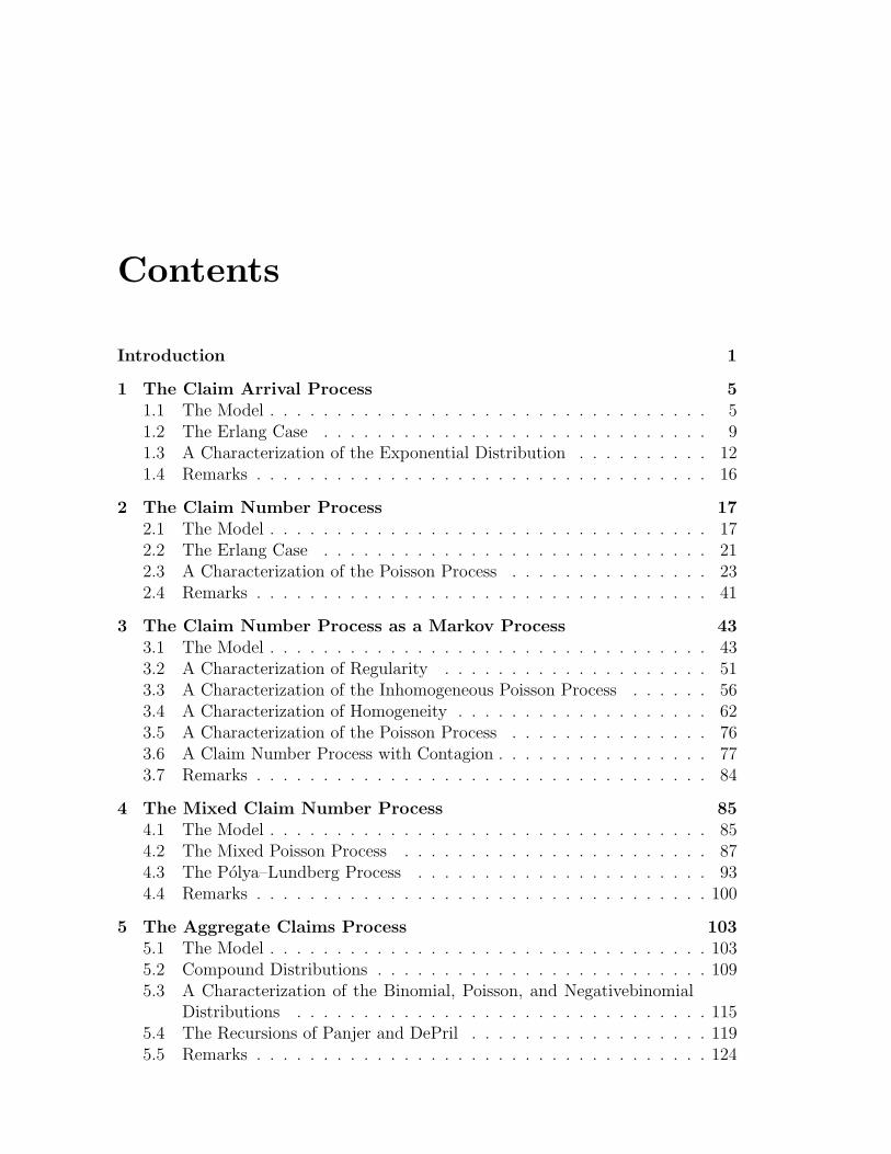
Contents
Introduction 1
1 The Claim Arrival Process 51.1 The Model . . . . . . . . . . . . . . . . . . . . . . . . . . . . . . . . . 51.2 The Erlang Case . . . . . . . . . . . . . . . . . . . . . . . . . . . . . 91.3 A Characterization of the Exponential Distribution . . . . . . . . . . 121.4 Remarks . . . . . . . . . . . . . . . . . . . . . . . . . . . . . . . . . . 16
2 The Claim Number Process 172.1 The Model . . . . . . . . . . . . . . . . . . . . . . . . . . . . . . . . . 172.2 The Erlang Case . . . . . . . . . . . . . . . . . . . . . . . . . . . . . 212.3 A Characterization of the Poisson Process . . . . . . . . . . . . . . . 232.4 Remarks . . . . . . . . . . . . . . . . . . . . . . . . . . . . . . . . . . 41
3 The Claim Number Process as a Markov Process 433.1 The Model . . . . . . . . . . . . . . . . . . . . . . . . . . . . . . . . . 433.2 A Characterization of Regularity . . . . . . . . . . . . . . . . . . . . 513.3 A Characterization of the Inhomogeneous Poisson Process . . . . . . 563.4 A Characterization of Homogeneity . . . . . . . . . . . . . . . . . . . 623.5 A Characterization of the Poisson Process . . . . . . . . . . . . . . . 763.6 A Claim Number Process with Contagion . . . . . . . . . . . . . . . . 773.7 Remarks . . . . . . . . . . . . . . . . . . . . . . . . . . . . . . . . . . 84
4 The Mixed Claim Number Process 854.1 The Model . . . . . . . . . . . . . . . . . . . . . . . . . . . . . . . . . 854.2 The Mixed Poisson Process . . . . . . . . . . . . . . . . . . . . . . . 874.3 The Polya–Lundberg Process . . . . . . . . . . . . . . . . . . . . . . 934.4 Remarks . . . . . . . . . . . . . . . . . . . . . . . . . . . . . . . . . . 100
5 The Aggregate Claims Process 1035.1 The Model . . . . . . . . . . . . . . . . . . . . . . . . . . . . . . . . . 1035.2 Compound Distributions . . . . . . . . . . . . . . . . . . . . . . . . . 1095.3 A Characterization of the Binomial, Poisson, and Negativebinomial
Distributions . . . . . . . . . . . . . . . . . . . . . . . . . . . . . . . 1155.4 The Recursions of Panjer and DePril . . . . . . . . . . . . . . . . . . 1195.5 Remarks . . . . . . . . . . . . . . . . . . . . . . . . . . . . . . . . . . 124
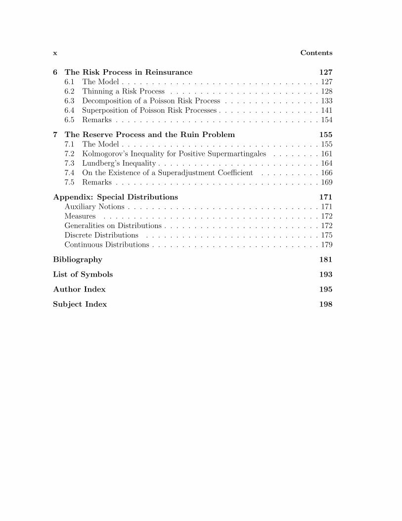
x Contents
6 The Risk Process in Reinsurance 1276.1 The Model . . . . . . . . . . . . . . . . . . . . . . . . . . . . . . . . . 1276.2 Thinning a Risk Process . . . . . . . . . . . . . . . . . . . . . . . . . 1286.3 Decomposition of a Poisson Risk Process . . . . . . . . . . . . . . . . 1336.4 Superposition of Poisson Risk Processes . . . . . . . . . . . . . . . . . 1416.5 Remarks . . . . . . . . . . . . . . . . . . . . . . . . . . . . . . . . . . 154
7 The Reserve Process and the Ruin Problem 1557.1 The Model . . . . . . . . . . . . . . . . . . . . . . . . . . . . . . . . . 1557.2 Kolmogorov’s Inequality for Positive Supermartingales . . . . . . . . 1617.3 Lundberg’s Inequality . . . . . . . . . . . . . . . . . . . . . . . . . . . 1647.4 On the Existence of a Superadjustment Coefficient . . . . . . . . . . 1667.5 Remarks . . . . . . . . . . . . . . . . . . . . . . . . . . . . . . . . . . 169
Appendix: Special Distributions 171Auxiliary Notions . . . . . . . . . . . . . . . . . . . . . . . . . . . . . . . . 171Measures . . . . . . . . . . . . . . . . . . . . . . . . . . . . . . . . . . . . 172Generalities on Distributions . . . . . . . . . . . . . . . . . . . . . . . . . . 172Discrete Distributions . . . . . . . . . . . . . . . . . . . . . . . . . . . . . 175Continuous Distributions . . . . . . . . . . . . . . . . . . . . . . . . . . . . 179
Bibliography 181
List of Symbols 193
Author Index 195
Subject Index 198
Introduction
Modelling the development in time of an insurer’s portfolio of risks is not an easy tasksince such models naturally involve various stochastic processes; this is especiallytrue in nonlife insurance where, in constrast with whole life insurance, not only theclaim arrival times are random but the claim severities are random as well.
The sequence of claim arrival times and the sequence of claim severities, the claimarrival process and the claim size process, constitute the two components of therisk process describing the development in time of the expenses for the portfoliounder consideration. The claim arrival process determines, and is determined by,the claim number process describing the number of claims occurring in any timeinterval. Since claim numbers are integervalued random variables whereas, in thecontinuous time model, claim arrival times are realvalued, the claim number processis, in principle, more accessible to statistical considerations.
As a consequence of the equivalence of the claim arrival process and the claimnumber process, the risk process is determined by the claim number process andthe claim size process. The collective point of view in risk theory considers onlythe arrival time and the severity of a claim produced by the portfolio but neglectsthe individual risk (or policy) causing the claim. It is therefore not too harmful toassume that the claim severities in the portfolio are i. i. d. so that their distributioncan easily be estimated from observations. As noticed by Kupper(1) [1962], thismeans that the claim number process is much more interesting than the claim sizeprocess. Also, Helten and Sterk(2) [1976] pointed out that the separate analysis ofthe claim number process and the claim size process leads to better estimates of the
(1)Kupper [1962]: Die Schadenversicherung . . . basiert auf zwei stochastischen Grossen, derSchadenzahl und der Schadenhohe. Hier tritt bereits ein fundamentaler Unterschied zur Lebensver-sicherung zutage, wo die letztere in den weitaus meisten Fallen eine zum voraus festgelegte, festeZahl darstellt. Die interessantere der beiden Variablen ist die Schadenzahl.(2)Helten and Sterk [1976]: Die Risikotheorie befaßt sich also zunachst nicht direkt mit derstochastischen Gesetzmaßigkeit des Schadenbedarfs, der aus der stochastischen Gesetzmaßigkeitder Schadenhaufigkeit und der Schadenausbreitung resultiert, denn ein Schadenbedarf . . . kannja in sehr verschiedener Weise aus Schadenhaufigkeit und Schadenhohe resultieren . . . Fur dieK–Haftpflicht zeigt eine Untersuchung von Troblinger [1975 ] sehr deutlich, daß eine Aufspaltungdes Schadenbedarfs in Schadenhaufigkeit und Schadenhohe wesentlich zur besseren Schatzung desSchadenbedarfs beitragen kann.
2 Introduction
aggregate claims amount, that is, the (random) sum of all claim severities occurringin some time interval.
The present book is devoted to the claim number process and also, to some extent, toits relatives, the aggregate claims process, the risk process, and the reserve process.The discussion of various classes of claim number processes will be rather detailedsince familiarity with a variety of properties of potential models is essential for modelselection. Of course, no mathematical model will ever completely match reality, butanalyzing models and confronting their properties with observations is an approvedway to check assumptions and to acquire more insight into real situations.
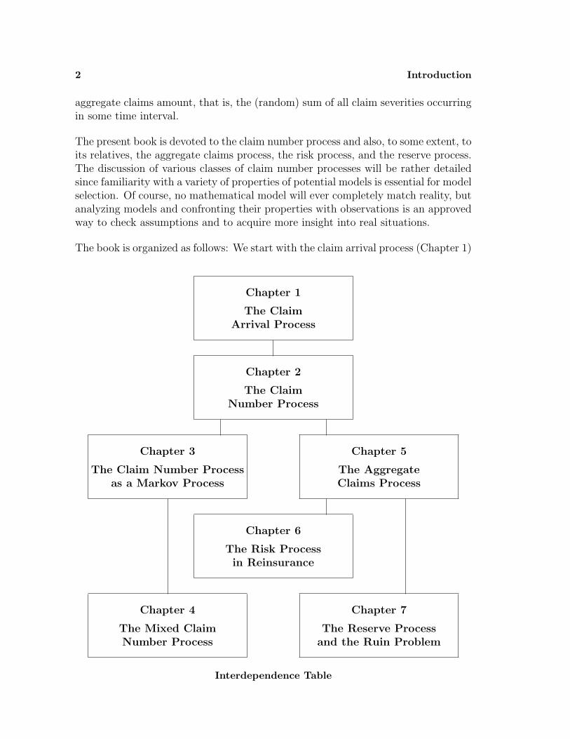
The book is organized as follows: We start with the claim arrival process (Chapter 1)
Chapter 1
The ClaimArrival Process
Chapter 2
The ClaimNumber Process
Chapter 3
The Claim Number Processas a Markov Process
Chapter 5
The AggregateClaims Process
Chapter 6
The Risk Processin Reinsurance
Chapter 4
The Mixed ClaimNumber Process
Chapter 7
The Reserve Processand the Ruin Problem
Interdependence Table
Introduction 3
and then turn to the claim number process which will be studied in three chapters,exhibiting the properties of the Poisson process (Chapter 2) and of its extensionsto Markov claim number processes (Chapter 3) and to mixed Poisson processes(Chapter 4). Mixed Poisson processes are particularly useful in applications sincethey reflect the idea of an inhomogeneous portfolio. We then pass to the aggregateclaims process and study some methods of computing or estimating aggregate claimsdistributions (Chapter 5). A particular aggregate claims process is the thinned claimnumber process occurring in excess of loss reinsurance, where the reinsurer assumesresponsibility for claim severities exceeding a given priority, and this leads to thediscussion of thinning and the related problems of decomposition and superpositionof risk processes (Chapter 6). Finally, we consider the reserve process and the ruinproblem in an infinite time horizon when the premium income is proportional totime (Chapter 7).
The Interdependence Table given above indicates various possibilities for a selectivereading of the book. For a first reading, it would be sufficient to study Chapters 1,2, 5, and 7, but it should be noted that Chapter 2 is almost entirely devoted to thePoisson process. Since Poisson processes are unrealistic models in many classes ofnonlife insurance, these chapters should be complemented by some of the materialpresented in Chapters 3, 4, and 6. A substantial part of Chapter 4 is independentof Chapter 3, and Chapters 6 and 7 contain only sporadic references to definitionsor results of Chapter 3 and depend on Chapter 5 only via Section 5.1. Finally, areader who is primarily interested in claim number processes may leave Chapter 5after Section 5.1 and omit Chapter 7.
The reader of these notes is supposed to have a solid background in abstract measureand integration theory as well as some knowledge in measure theoretic probabilitytheory; by contrast, particular experience with special distributions or stochasticprocesses is not required. All prerequisites can be found in the monographs byAliprantis and Burkinshaw [1990], Bauer [1991, 1992], and Billingsley [1995].
Almost all proofs are given in great detail; some of them are elementary, othersare rather involved, and certain proofs may seem to be superfluous since the resultis suggested by the actuarial interpretation of the model. However, if actuarialmathematics is to be considered as a part of probability theory and mathematicalstatistics, then it has to accept its (sometimes bothering) rigour.
The notation in this book is standard, but for the convenience of the reader we fixsome symbols and conventions; further details on notation may be found in the Listof Symbols.
Throughout this book, let (Ω,F , P ) be a fixed probability space, let B(Rn) denotethe σ–algebra of Borel sets on the Euclidean space Rn, let ξ denote the countingmeasure concentrated on N0, and let λn denote the Lebesgue measure on B(Rn);in the case n = 1, the superscript n will be dropped.
4 Introduction
The indicator function of a set A will be denoted by χA. A family of sets Aii∈I issaid to be disjoint if it is pairwise disjoint, and in this case its union will be denotedby
∑i∈I Ai. A family of sets Aii∈I is said to be a partition of A if it is disjoint
and satisfies∑
i∈I Ai = A.
For a sequence of random variables Znn∈N which are i. i. d. (independent andidentically distributed), a typical random variable of the sequence will be denotedby Z. As a rule, integrals are Lebesgue integrals, but occasionally we have to switchto Riemann integrals in order to complete computations.
In some cases, sums, products, intersections, and unions extend over the emptyindex set; in this case, they are defined to be equal to zero, one, the reference set,and the empty set, respectively. The terms positive, increasing, etc. are used in theweak sense admitting equality.
The main concepts related to (probability) distributions as well as the definitionsand the basic properties of the distributions referred to by name in this book arecollected in the Appendix. Except for the Dirac distributions, all parametric familiesof distributions are defined as to exclude degenerate distributions and such that theirparameters are taken from open intervals of R or subsets of N.
It has been pointed out before that the present book addresses only a single topic ofrisk theory: The development in time of a fixed portfolio of risks. Other importanttopics in risk theory include the approximation of aggregate claims distributions,tariffication, reserving, and reinsurance, as well as the wide field of life insurance or,more generally, insurance of persons. The following references may serve as a guideto recent publications on some topics of actuarial mathematics which are beyondthe scope of this book:– Life insurance mathematics : Gerber [1986, 1990, 1995], Wolfsdorf [1986], Wolt-
huis [1994], and Helbig and Milbrodt [1995].– Life and nonlife insurance mathematics : Bowers, Gerber, Hickman, Jones, and
Nesbitt [1986], Panjer and Willmot [1992], and Daykin, Pentikainen and Pesonen[1994].
– Nonlife insurance mathematics : Buhlmann [1970], Gerber [1979], Sundt [1984,1991, 1993], Heilmann [1987, 1988], Straub [1988], Wolfsdorf [1988], Goovaerts,Kaas, van Heerwaarden, and Bauwelinckx [1990], Hipp and Michel [1990], andNorberg [1990].
Since the traditional distinction between life and nonlife insurance mathematics isbecoming more and more obsolete, future research in actuarial mathematics should,in particular, aim at a unified theory providing models for all classes of insurance.
Chapter 1
The Claim Arrival Process
In order to model the development of an insurance business in time, we proceed inseveral steps by successively introducing– the claim arrival process,– the claim number process,– the aggregate claims process, and– the reserve process.We shall see that claim arrival processes and claim number processes determine eachother, and that claim number processes are the heart of the matter.
The present chapter is entirely devoted to the claim arrival process.
We first state the general model which will be studied troughout this book andwhich will be completed later (Section 1.1). We then study the special case of aclaim arrival process having independent and identically exponentially distributedwaiting times between two successive claims (Section 1.2). We finally show that theexponential distribution is of particular interest since it is the unique distributionwhich is memoryless on the interval (0,∞) (Section 1.3).
1.1 The Model
We consider a portfolio of risks which are insured by some insurer. The risks produceclaims and pay premiums to the insurer who, in turn, will settle the claims. Theportfolio may consist of a single risk or of several ones.
We assume that the insurer is primarily interested in the overall performance of theportfolio, that is, the balance of premiums and claim payments aggregated over allrisks. (Of course, a surplus of premiums over claim payments would be welcome!)In the case where the portfolio consists of several risks, this means that the insurerdoes not care which of the risks in the portfolio causes a particular claim. This isthe collective point of view in risk theory.
6 Chapter 1 The Claim Arrival Process
We assume further that in the portfolio claims occur at random in an infinite timehorizon starting at time zero such that– no claims occur at time zero, and– no two claims occur simultaneously.The assumption of no two claims occurring simultaneously seems to be harmless.Indeed, it should not present a serious problem when the portfolio is small; however,when the portfolio is large, it depends on the class of insurance under considerationwhether this assumption is really acceptable. (For example, the situation is certainlydifferent in fire insurance and in (third party liability) automobile insurance, where incertain countries a single insurance company holds about one quarter of all policies;in such a situation, one has to take into account the possibility that two insureesfrom the same large portfolio produce a car accident for which both are responsiblein parts.)
Comment: When the assumption of no two claims occurring simultaneously isjudged to be non–acceptable, it can nevertheless be saved by slightly changing thepoint of view, namely, by considering claim events (like car accidents) instead ofsingle claims. The number of single claims occurring at a given claim event can thenbe interpreted as the size of the claim event. This point of view will be discussedfurther in Chapter 5 below.
Let us now transform the previous ideas into a probabilistic model:
A sequence of random variables Tnn∈N0is a claim arrival process if there exists a
null set ΩT ∈ F such that, for all ω ∈ Ω\ΩT ,– T0(ω) = 0 and– Tn−1(ω) < Tn(ω) holds for all n ∈ N.Then we have Tn(ω) > 0 for all n ∈ N and all ω ∈ Ω\ΩT . The null set ΩT is saidto be the exceptional null set of the claim arrival process Tnn∈N0
.
For a claim arrival process Tnn∈N0and for all n ∈ N, define the increment
Wn := Tn − Tn−1 .
Then we have Wn(ω) > 0 for all n ∈ N and all ω ∈ Ω\ΩT , and hence
E[Wn] > 0
for all n ∈ N, as well as
Tn =n∑
k=1
Wk
for all n ∈ N. The sequence Wnn∈N is said to be the claim interarrival processinduced by the claim arrival process Tnn∈N0
.
1.1 The Model 7
Interpretation:– Tn is the occurrence time of the nth claim.– Wn is the waiting time between the occurrence of claim n−1 and the occurrence
of claim n.– With probability one, no claim occurs at time zero and no two claims occur
simultaneously.
For the remainder of this chapter, let Tnn∈N0be a fixed claim arrival process and
let Wnn∈N be the claim interarrival process induced by Tnn∈N0. Without loss of
generality, we may and do assume that the exceptional null set of the claim arrivalprocess is empty.
Since Wn = Tn − Tn−1 and Tn =∑n
k=1 Wn holds for all n ∈ N, it is clear that theclaim arrival process and the claim interarrival process determine each other. Inparticular, we have the following obvious but useful result:
1.1.1 Lemma. The identity
σ(Tkk∈0,1,...,n
)= σ
(Wkk∈1,...,n)
holds for all n∈N.
Furthermore, for n ∈ N, let Tn and Wn denote the random vectors Ω → Rn withcoordinates Ti and Wi, respectively, and let Mn denote the (n×n)–matrix withentries
mij :=
1 if i ≥ j0 if i < j .
Then Mn is invertible and satisfies detMn = 1, and we have Tn = Mn Wn andWn = M−1
n Tn. The following result is immediate:
1.1.2 Lemma. For all n∈N, the distributions of Tn and Wn satisfy
PTn= (PWn
)Mnand PWn
= (PTn)M−1
n.
The assumptions of our model do not exclude the possibility that infinitely manyclaims occur in finite time. The event
supn∈N Tn < ∞is called explosion.
1.1.3 Lemma. If supn∈N E[Tn] < ∞, then the probability of explosion is equal toone.
This is obvious from the monotone convergence theorem.
8 Chapter 1 The Claim Arrival Process
1.1.4 Corollary. If∑∞
n=1 E[Wn] < ∞, then the probability of explosion is equalto one.
In modelling a particular insurance business, one of the first decisions to take is todecide whether the probability of explosion should be zero or not. This decision is,of course, a decision concerning the distribution of the claim arrival process.
We conclude this section with a construction which in the following chapter willturn out to be a useful technical device:
For n ∈ N, the graph of Tn is defined to be the map Un : Ω → Ω×R, given by
Un(ω) :=(ω, Tn(ω)
).
Then each Un is F–F⊗B(R)–measurable. Define a measure µ : F⊗B(R) → [0,∞]by letting
µ[C] :=∞∑
n=1
PUn [C] .
The measure µ will be called the claim measure induced by the claim arrival processTnn∈N0
.
1.1.5 Lemma. The identity
µ[A×B] =
∫
A
( ∞∑n=1
χTn∈B
)dP
holds for all A ∈ F and B ∈ B(R).
Proof. Since U−1n (A×B) = A ∩ Tn∈B, we have
µ[A×B] =∞∑
n=1
PUn [A×B]
=∞∑
n=1
P [A ∩ Tn∈B]
=∞∑
n=1
∫
A
χTn∈B dP
=
∫
A
( ∞∑n=1
χTn∈B
)dP ,
as was to be shown. 2
The previous result connects the claim measure with the claim number process whichwill be introduced in Chapter 2.
1.2 The Erlang Case 9
Most results in this book involving special distributions concern the case where thedistributions of the claim arrival times are absolutely continuous with respect toLebesgue measure; this case will be referred to as the continuous time model. It is,however, quite interesting to compare the results for the continuous time model withcorresponding ones for the case where the distributions of the claim arrival timesare absolutely continuous with respect to the counting measure concentrated on N0.In the latter case, there is no loss of generality if we assume that the claim arrivaltimes are integer–valued, and this case will be referred to as the discrete time model.The discrete time model is sometimes considered to be an approximation of thecontinuous time model if the time unit is small, but we shall see that the propertiesof the discrete time model may drastically differ from those of the continuous timemodel. On the other hand, the discrete time model may also serve as a simplemodel in its own right if the portfolio is small and if the insurer merely wishes todistinguish claim–free periods from periods with a strictly positive number of claims.Results for the discrete time model will be stated as problems in this and subsequentchapters.
Another topic which is related to our model is life insurance. In the simplest case, weconsider a single random variable T satisfying P [T > 0] = 1, which is interpretedas the time of death or the lifetime of the insured individual; accordingly, this modelis called single life insurance. More generally, we consider a finite sequence of randomvariables Tnn∈0,1,...,N satisfying P [T0 = 0] = 1 and P [Tn−1 < Tn] = 1 for alln ∈ 1, . . . , N, where Tn is interpreted as the time of the nth death in a portfolioof N insured individuals; accordingly, this model is called multiple life insurance.Although life insurance will not be studied in detail in these notes, some aspects ofsingle or multiple life insurance will be discussed as problems in this and subsequentchapters.
Problems1.1.A If the sequence of claim interarrival times is i. i. d., then the probability of explo-
sion is equal to zero.
1.1.B Discrete Time Model: The inequality Tn ≥ n holds for all n ∈ N.
1.1.C Discrete Time Model: The probability of explosion is equal to zero.
1.1.D Multiple Life Insurance: Extend the definition of a claim arrival process asto cover the case of multiple (and hence single) life insurance.
1.1.E Multiple Life Insurance: The probability of explosion is equal to zero.
1.2 The Erlang Case
In some of the special cases of our model which we shall discuss in detail, the claiminterarrival times are assumed or turn out to be independent and exponentially
10 Chapter 1 The Claim Arrival Process
distributed. In this situation, explosion is either impossible or certain:
1.2.1 Theorem (Zero–One Law on Explosion). Let αnn∈N be a sequenceof real numbers in (0,∞) and assume that the sequence of claim interarrival timesWnn∈N is independent and satisfies PWn = Exp(αn) for all n∈N.(a) If the series
∑∞n=1 1/αn diverges, then the probability of explosion is equal to
zero.(b) If the series
∑∞n=1 1/αn converges, then the probability of explosion is equal to
one.
Proof. By the dominated convergence theorem, we have
E[e−
∑∞n=1
Wn
]= E
[ ∞∏n=1
e−Wn
]
=∞∏
n=1
E[e−Wn
]
=∞∏
n=1
αn
αn + 1
=∞∏
n=1
(1− 1
1 + αn
)
≤∞∏
n=1
e−1/(1+αn)
= e−∑∞
n=11/(1+αn) .
Thus, if the series∑∞
n=1 1/αn diverges, then the series∑∞
n=1 1/(1+αn) diverges aswell and we have P [∑∞
n=1 Wn = ∞] = 1, and thus
P [supn∈N Tn < ∞] = P
[ ∞∑n=1
Wn < ∞]
= 0 ,
which proves (a).Assertion (b) is immediate from Corollary 1.1.4. 2
In the case of independent claim interarrival times, the following result is also ofinterest:
1.2.2 Lemma. Let α ∈ (0,∞). If the sequence of claim interarrival times Wnn∈Nis independent, then the following are equivalent :(a) PWn = Exp(α) for all n∈N.(b) PTn = Ga(α, n) for all n∈N.In this case, E[Wn] = 1/α and E[Tn] = n/α holds for all n∈N, and the probabilityof explosion is equal to zero.
1.2 The Erlang Case 11
Proof. The simplest way to prove the equivalence of (a) and (b) is to use charac-teristic functions.• Assume first that (a) holds. Since Tn =
∑nk=1 Wk, we have
ϕTn(z) =n∏
k=1
ϕWk(z)
=n∏
k=1
α
α− iz
=
(α
α− iz
)n
,
and thus PTn = Ga(α, n). Therefore, (a) implies (b).• Assume now that (b) holds. Since Tn−1 + Wn = Tn, we have
(α
α− iz
)n−1
· ϕWn(z) = ϕTn−1(z) · ϕWn(z)
= ϕTn(z)
=
(α
α− iz
)n
,
hence
ϕWn(z) =α
α− iz,
and thus PWn = Exp(α). Therefore, (b) implies (a).• The final assertion is obvious from the distributional assumptions and the zero–one law on explosion.• For readers not familiar with characteristic functions, we include an elementaryproof of the implication (a) =⇒ (b); only this implication will be needed in thesequel. Assume that (a) holds. We proceed by induction.Obviously, since T1 = W1 and Exp(α) = Ga(α, 1), we have PT1 = Ga(α, 1).Assume now that PTn = Ga(α, n) holds for some n ∈ N. Then we have
PTn [B] =
∫
B
αn
Γ(n)e−αx xn−1χ(0,∞)(x) dλ(x)
and
PWn+1 [B] =
∫
B
αe−αxχ(0,∞)(x) dλ(x)
for all B ∈ B(R). Since Tn and Wn+1 are independent, the convolution formulayields
PTn+1 [B] = PTn+Wn+1 [B]
= PTn ∗ PWn+1 [B]
12 Chapter 1 The Claim Arrival Process
=
∫
B
(∫
R
αn
Γ(n)e−α(t−s)(t−s)n−1χ(0,∞)(t−s) αe−αsχ(0,∞)(s) dλ(s)
)dλ(t)
=
∫
B
αn+1
Γ(n+1)e−αt
(∫
Rn(t−s)n−1χ(0,t)(s) dλ(s)
)χ(0,∞)(t) dλ(t)
=
∫
B
αn+1
Γ(n+1)e−αt
(∫ t
0
n(t−s)n−1 ds
)χ(0,∞)(t) dλ(t)
=
∫
B
αn+1
Γ(n+1)e−αt tn χ(0,∞)(t) dλ(t)
=
∫
B
αn+1
Γ(n+1)e−αt t(n+1)−1χ(0,∞)(t) dλ(t)
for all B ∈ B(R), and thus PTn+1 = Ga(α, n+1). Therefore, (a) implies (b). 2
The particular role of the exponential distribution will be discussed in the followingsection.
Problems1.2.A Let Q := Exp(α) for some α ∈ (0,∞) and let Q′ denote the unique distribution
satisfying Q′[k] = Q[(k−1, k]] for all k ∈ N. Then Q′ = Geo(1−e−α).
1.2.B Discrete Time Model: Let ϑ∈(0, 1). If the sequence Wnn∈N is independent,then the following are equivalent:(a) PWn = Geo(ϑ) for all n ∈ N.(b) PTn = Geo(n, ϑ) for all n ∈ N.In this case, E[Wn] = 1/ϑ and E[Tn] = n/ϑ holds for all n ∈ N.
1.3 A Characterization of the ExponentialDistribution
One of the most delicate problems in probabilistic modelling is the appropriatechoice of the distributions of the random variables in the model. More precisely, itis the joint distribution of all random variables that has to be specified. To make thischoice, it is useful to know that certain distributions are characterized by generalproperties which are easy to interpret.
In the model considered here, it is sufficient to specify the distribution of the claiminterarrival process. This problem is considerably reduced if the claim interarrivaltimes are assumed to be independent, but even in that case the appropriate choiceof the distributions of the single claim interarrival times is not obvious. In whatfollows we shall characterize the exponential distribution by a simple property which
1.3 A Characterization of the Exponential Distribution 13
is helpful to decide whether or not in a particular insurance business this distributionis appropriate for the claim interarrival times.
For the moment, consider a random variable W which may be interpreted as awaiting time.
If PW = Exp(α), then the survival function R → [0, 1] : w 7→ P [W > w] of thedistribution of W satisfies P [W > w] = e−αw for all w ∈ R+, and this yields
P [W > s+t] = P [W > s] · P [W > t]
or, equivalently,
P [W > s+t|W > s] = P [W > t]
for all s, t ∈ R+. The first identity reflects the fact that the survival function of theexponential distribution is self–similar on R+ in the sense that, for each s ∈ R+,the graphs of the mappings t 7→ P [W > s+t] and t 7→ P [W > t] differ only bya scaling factor. Moreover, if W is interpreted as a waiting time, then the secondidentity means that the knowledge of having waited more than s time units doesnot provide any information on the remaining waiting time. Loosely speaking, theexponential distribution has no memory (or does not use it). The question ariseswhether the exponential distribution is the unique distribution having this property.
Before formalizing the notion of a memoryless distribution, we observe that in thecase PW = Exp(α) the above identities hold for all s, t ∈ R+ but fail for all s, t ∈ Rsuch that s < 0 < s+t; on the other hand, we have PW [R+] = 1. These observationslead to the following definition:
A distribution Q : B(R) → [0, 1] is memoryless on S ∈ B(R) if– Q[S] = 1 and– the identity
Q[(s+t,∞)] = Q[(s,∞)] ·Q[(t,∞)]
holds for all s, t ∈ S.The following result yields a general property of memoryless distributions:
1.3.1 Theorem. Let Q : B(R) → [0, 1] be a distribution which is memoryless onS ∈ B(R). If 0∈S, then Q satisfies either Q[0] = 1 or Q[(0,∞)] = 1.
Proof. Assume that Q[(0,∞)] < 1. Since 0 ∈ S, we have
Q[(0,∞)] = Q[(0,∞)] ·Q[(0,∞)]
= Q[(0,∞)]2 ,
14 Chapter 1 The Claim Arrival Process
hence
Q[(0,∞)] = 0 ,
and thus
Q[(t,∞)] = Q[(t,∞)] ·Q[(0,∞)]
= 0
for all t ∈ S.Define t := inf S and choose a sequence tnn∈N ⊆ S which decreases to t. Then wehave
Q[(t,∞)] = supn∈N Q[(tn,∞)]
= 0 .
Since Q[S] = 1, we also have
Q[(−∞, t)] = 0 .
Therefore, we have
Q[t] = 1 ,
hence Q[t ∩ S] = 1, and thus t ∈ S.Finally, since 0 ∈ S, we have either t < 0 or t = 0. But t < 0 implies t ∈ (2t,∞)and hence
Q[t] ≤ Q[(2t,∞)]
= Q[(t,∞)] ·Q[(t,∞)]
= Q[(t,∞)]2 ,
which is impossible. Therefore, we have t = 0 and hence Q[0] = 1, as was to beshown. 2
The following result characterizes the exponential distribution:
1.3.2 Theorem. For a distribution Q : B(R) → [0, 1], the following are equivalent :(a) Q is memoryless on (0,∞).(b) Q = Exp(α) for some α ∈ (0,∞).In this case, α = − log Q[(1,∞)].
Proof. Note that Q = Exp(α) if and only if the identity
Q[(t,∞)] = e−αt
holds for all t ∈ [0,∞).
1.3 A Characterization of the Exponential Distribution 15
• Assume that (a) holds. By induction, we have
Q[(n,∞)] = Q[(1,∞)]n
and
Q[(1,∞)] = Q[(1/n,∞)]n
for all n ∈ N.Thus, Q[(1,∞)] = 1 is impossible because of
0 = Q[∅]= infn∈N Q[(n,∞)]
= infn∈N Q[(1,∞)]n ,
and Q[(1,∞)] = 0 is impossible because of
1 = Q[(0,∞)]
= supn∈N Q[(1/n,∞)]
= supn∈N Q[(1,∞)]1/n .
Therefore, we have
Q[(1,∞)] ∈ (0, 1) .
Define now α := − log Q[(1,∞)]. Then we have α ∈ (0,∞) and
Q[(1,∞)] = e−α ,
and thus
Q[(m/n,∞)] = Q[(1,∞)]m/n
=(e−α
)m/n
= e−αm/n
for all m, n ∈ N. This yields
Q[(t,∞)] = e−αt
for all t ∈ (0,∞) ∩ Q. Finally, for each t ∈ [0,∞) we may choose a sequencetnn∈N ⊆ (0,∞) ∩Q which decreases to t, and we obtain
Q[(t,∞)] = supn∈N Q[(tn,∞)]
= supn∈N e−αtn
= e−αt .
By the introductory remark, it follows that Q = Exp(α). Therefore, (a) implies (b).• The converse implication is obvious. 2
16 Chapter 1 The Claim Arrival Process
1.3.3 Corollary. For a distribution Q : B(R) → [0, 1], the following are equivalent :(a) Q is memoryless on R+.(b) Either Q = δ0 or Q = Exp(α) for some α ∈ (0,∞).
Proof. The assertion is immediate from Theorems 1.3.1 and 1.3.2. 2
With regard to the previous result, note that the Dirac distribution δ0 is the limitof the exponential distributions Exp(α) as α →∞.
1.3.4 Corollary. There is no distribution which is memoryless on R.
Proof. If Q : B(R) → [0, 1] is a distribution which is memoryless on R, theneither Q = δ0 or Q = Exp(α) for some α ∈ (0,∞), by Theorem 1.3.1 and Corollary1.3.3. On the other hand, none of these distributions is memoryless on R. 2
Problems1.3.A Discrete Time Model: For a distribution Q : B(R) → [0, 1], the following are
equivalent:(a) Q is memoryless on N.(b) Either Q = δ1 or Q = Geo(ϑ) for some ϑ ∈ (0, 1).Note that the Dirac distribution δ1 is the limit of the geometric distributionsGeo(ϑ) as ϑ → 0.
1.3.B Discrete Time Model: For a distribution Q : B(R) → [0, 1], the following areequivalent:(a) Q is memoryless on N0.(b) Either Q = δ0 or Q = δ1 or Q = Geo(ϑ) for some ϑ ∈ (0, 1).In particular, the negativebinomial distribution fails to be memoryless on N0.
1.3.C There is no distribution which is memoryless on (−∞, 0).
1.4 Remarks
Since the conclusions obtained in a probabilistic model usually concern probabilitiesand not single realizations of random variables, it is natural to state the assump-tions of the model in terms of probabilities as well. While this is a merely formaljustification for the exceptional null set in the definition of the claim arrival process,there is also a more substantial reason: As we shall see in Chapters 5 and 6 below,it is sometimes of interest to construct a claim arrival process from other randomvariables, and in that case it cannot in general be ensured that the exceptional nullset is empty.
Theorem 1.3.2 is the most famous characterization of the exponential distribution.Further characterizations of the exponential distribution can be found in the mono-graphs by Galambos and Kotz [1978] and, in particular, by Azlarov and Volodin[1986].
Chapter 2
The Claim Number Process
In the previous chapter, we have formulated a general model for the occurrence ofclaims in an insurance business and we have studied the claim arrival process insome detail.
In the present chapter, we proceed one step further by introducing the claim numberprocess. Particular attention will be given to the Poisson process.
We first introduce the general claim number process and show that claim numberprocesses and claim arrival processes determine each other (Section 2.1). We thenestablish a connection between certain assumptions concerning the distributions ofthe claim arrival times and the distributions of the claim numbers (Section 2.2). Wefinally prove the main result of this chapter which characterizes the (homogeneous)Poisson process in terms of the claim interarrival process, the claim measure, and amartingale property (Section 2.3).
2.1 The Model
A family of random variables Ntt∈R+is a claim number process if there exists a
null set ΩN ∈ F such that, for all ω ∈ Ω\ΩN ,– N0(ω) = 0,– Nt(ω) ∈ N0∪∞ for all t ∈ (0,∞),– Nt(ω) = infs∈(t,∞) Ns(ω) for all t ∈ R+,– sups∈[0,t) Ns(ω) ≤ Nt(ω) ≤ sups∈[0,t) Ns(ω) + 1 for all t ∈ R+, and– supt∈R+
Nt(ω) = ∞.The null set ΩN is said to be the exceptional null set of the claim number processNtt∈R+
.
Interpretation:– Nt is the number of claims occurring in the interval (0, t].– Almost all paths of Ntt∈R+
start at zero, are right–continuous, increase withjumps of height one at discontinuity points, and increase to infinity.
18 Chapter 2 The Claim Number Process
Our first result asserts that every claim arrival process induces a claim numberprocess, and vice versa:
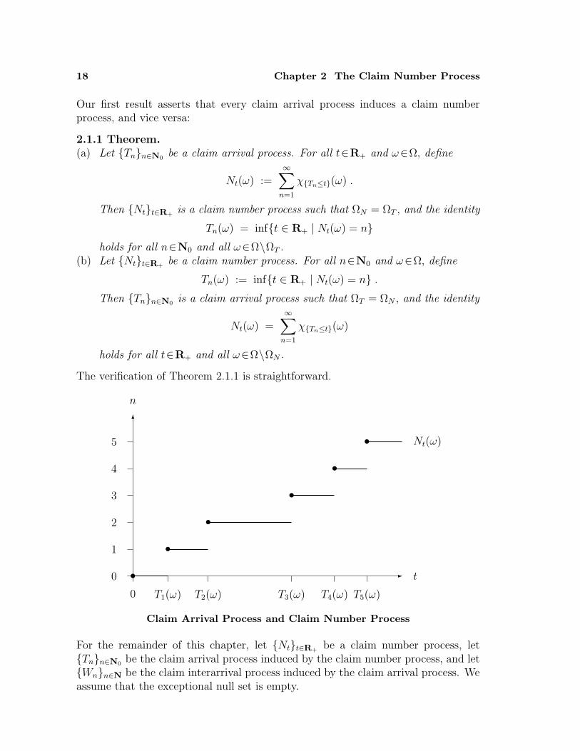
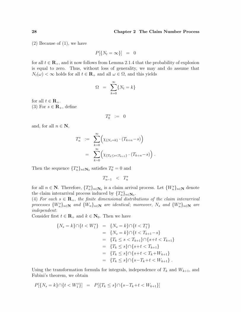
2.1.1 Theorem.(a) Let Tnn∈N0
be a claim arrival process. For all t∈R+ and ω∈Ω, define
Nt(ω) :=∞∑
n=1
χTn≤t(ω) .
Then Ntt∈R+is a claim number process such that ΩN = ΩT , and the identity
Tn(ω) = inft ∈ R+ | Nt(ω) = nholds for all n∈N0 and all ω∈Ω\ΩT .
(b) Let Ntt∈R+be a claim number process. For all n∈N0 and ω∈Ω, define
Tn(ω) := inft ∈ R+ | Nt(ω) = n .
Then Tnn∈N0is a claim arrival process such that ΩT = ΩN , and the identity
Nt(ω) =∞∑
n=1
χTn≤t(ω)
holds for all t∈R+ and all ω∈Ω\ΩN .
The verification of Theorem 2.1.1 is straightforward.
0 -
1
2
3
4
5
n
6
0 T1(ω) T2(ω) T3(ω) T4(ω) T5(ω)
t•
•
•
•
•
• Nt(ω)
Claim Arrival Process and Claim Number Process
For the remainder of this chapter, let Ntt∈R+be a claim number process, let
Tnn∈N0be the claim arrival process induced by the claim number process, and let
Wnn∈N be the claim interarrival process induced by the claim arrival process. Weassume that the exceptional null set is empty.
2.1 The Model 19
By virtue of the assumption that the exceptional null set is empty, we have twosimple but most useful identities, showing that certain events determined by theclaim number process can be interpreted as events determined by the claim arrivalprocess, and vice versa:
2.1.2 Lemma. The identities(a) Nt ≥ n = Tn ≤ t and(b) Nt = n = Tn ≤ t\Tn+1 ≤ t = Tn ≤ t < Tn+1hold for all n∈N0 and t∈R+.
The following result expresses in a particularly concise way the fact that the claimnumber process and the claim arrival process contain the same information:
2.1.3 Lemma.σ(Ntt∈R+
) = σ(Tnn∈N0) .
In view of the preceding discussion, it is not surprising that explosion can also beexpressed in terms of the claim number process:
2.1.4 Lemma. The probability of explosion satisfies
P [supn∈N Tn < ∞] = P
[⋃t∈N
Nt = ∞]
= P
[⋃t∈(0,∞)
Nt = ∞]
.
Proof. Since the family of sets Nt = ∞t∈(0,∞) is increasing, we have
⋃t∈(0,∞)
Nt = ∞ =⋃
t∈NNt = ∞ .
By Lemma 2.1.2, this yields
⋃t∈(0,∞)
Nt = ∞ =⋃
t∈NNt = ∞
=⋃
t∈N
⋂n∈N
Nt ≥ n=
⋃t∈N
⋂n∈N
Tn ≤ t=
⋃t∈N
supn∈N Tn ≤ t
= supn∈N Tn < ∞ ,
and the assertion follows. 2
2.1.5 Corollary. Assume that the claim number process has finite expectations.Then the probability of explosion is equal to zero.
Proof. By assumption, we have E[Nt] < ∞ and hence P [Nt =∞] = 0 for allt ∈ (0,∞). The assertion now follows from Lemma 2.1.4. 2
20 Chapter 2 The Claim Number Process
The discussion of the claim number process will to a considerable extent rely on theproperties of its increments which are defined as follows:
For s, t ∈ R+ such that s ≤ t, the increment of the claim number process Ntt∈R+
on the interval (s, t] is defined to be
Nt −Ns :=∞∑
n=1
χs<Tn≤t .
Since N0 = 0 and Tn > 0 for all n ∈N, this is in accordance with the definitionof Nt; in addition, we have
Nt(ω) = (Nt−Ns)(ω) + Ns(ω) ,
even if Ns(ω) is infinite.
The final result in this section connects the increments of the claim number process,and hence the claim number process itself, with the claim measure:
2.1.6 Lemma. The identity
µ[A×(s, t]] =
∫
A
(Nt−Ns) dP
holds for all A ∈ F and s, t ∈ R+ such that s ≤ t.
Proof. The assertion follows from Lemma 1.1.5 and the definition of Nt−Ns. 2
In the discrete time model, we have Nt = Nt+h for all t ∈ N0 and h∈ [0, 1) so thatnothing is lost if in this case the index set of the claim number process Ntt∈R+
isreduced to N0; we shall then refer to the sequence Nll∈N0
as the claim numberprocess induced by Tnn∈N0
.
Problems2.1.A Discrete Time Model: The inequalities
(a) Nl ≤ Nl−1+1 and(b) Nl ≤ lhold for all l ∈ N.
2.1.B Discrete Time Model: The identities(a) Nl−Nl−1 = 0 =
∑lj=1Tj−1 < l < Tj,
Nl−Nl−1 = 1 =∑l
j=1Tj = l, and(b) Tn = l = n ≤ Nl\n ≤ Nl−1 = Nl−1 < n ≤ Nlhold for all n ∈ N and l ∈ N.
2.2 The Erlang Case 21
2.1.C Multiple Life Insurance: For all t ∈ R+, define Nt :=∑N
n=1 χTn≤t. Thenthere exists a null set ΩN ∈ F such that, for all ω ∈ Ω\ΩN ,– N0(ω) = 0,– Nt(ω) ∈ 0, 1, . . . , N for all t ∈ (0,∞),– Nt(ω) = infs∈(t,∞) Ns(ω) for all t ∈ R+,– sups∈[0,t) Ns(ω) ≤ Nt(ω) ≤ sups∈[0,t) Ns(ω) + 1 for all t ∈ R+, and– supt∈R+
Nt(ω) = N .
2.2 The Erlang Case
In the present section we return to the special case of claim arrival times having anErlang distribution.
2.2.1 Lemma. Let α ∈ (0,∞). Then the following are equivalent :(a) PTn = Ga(α, n) for all n∈N.(b) PNt = P(αt) for all t∈(0,∞).In this case, E[Tn] = n/α holds for all n∈N and E[Nt] = αt holds for all t∈(0,∞).
Proof. Note that the identity
e−αt (αt)n
n!=
∫ t
0
αn
Γ(n)e−αssn−1 ds−
∫ t
0
αn+1
Γ(n+1)e−αssn ds
holds for all n ∈ N and t ∈ (0,∞).• Assume first that (a) holds. Lemma 2.1.2 yields
P[Nt = 0] = P
[t < T1]
= e−αt ,
and, for all n ∈ N,
P[Nt = n] = P
[Tn ≤ t]− P[Tn+1 ≤ t]
=
∫
(−∞,t]
αn
Γ(n)e−αssn−1χ(0,∞)(s) dλ(s)
−∫
(−∞,t]
αn+1
Γ(n+1)e−αss(n+1)−1χ(0,∞)(s) dλ(s)
=
∫ t
0
αn
Γ(n)e−αssn−1 ds−
∫ t
0
αn+1
Γ(n+1)e−αssn ds
= e−αt (αt)n
n!.
This yields
P[Nt = n] = e−αt (αt)n
n!
for all n ∈ N0, and hence PNt = P(αt). Therefore, (a) implies (b).
22 Chapter 2 The Claim Number Process
• Assume now that (b) holds. Since Tn > 0, we have
P[Tn ≤ t] = 0
for all t ∈ (−∞, 0]; also, for all t ∈ (0,∞), Lemma 2.1.2 yields
P[Tn ≤ t] = P
[Nt ≥ n]
= 1− P[Nt ≤ n−1]
= 1−n−1∑
k=0
P[Nt = k]
= 1−n−1∑
k=0
e−αt (αt)k
k!
= (1−e−αt)−n−1∑
k=1
e−αt (αt)k
k!
=
∫ t
0
αe−αs ds−n−1∑
k=1
(∫ t
0
αk
Γ(k)e−αssk−1 ds−
∫ t
0
αk+1
Γ(k+1)e−αssk ds
)
=
∫ t
0
αn
Γ(n)e−αssn−1 ds
=
∫
(−∞,t]
αn
Γ(n)e−αssn−1χ(0,∞)(s) dλ(s) .
This yields
P[Tn ≤ t] =
∫
(−∞,t]
αn
Γ(n)e−αssn−1χ(0,∞)(s) dλ(s)
for all t ∈ R, and hence PTn = Ga(α, n). Therefore, (b) implies (a).• The final assertion is obvious. 2
By Lemma 1.2.2, the equivalent conditions of Lemma 2.2.1 are fulfilled whenever theclaim interarrival times are independent and identically exponentially distributed;that case, however, can be characterized by a much stronger property of the claimnumber process involving its increments, as will be seen in the following section.
Problem2.2.A Discrete Time Model: Let ϑ ∈ (0, 1). Then the following are equivalent:
(a) PTn = Geo(n, ϑ) for all n ∈ N.(b) PNl
= B(l, ϑ) for all l ∈ N.In this case, E[Tn] = n/ϑ holds for all n ∈ N and E[Nl] = lϑ holds for all l ∈ N;moreover, for each l ∈ N, the pair (Nl−Nl−1, Nl−1) is independent and satisfiesPNl−Nl−1
= B(ϑ).
2.3 A Characterization of the Poisson Process 23
2.3 A Characterization of the Poisson Process
The claim number process Ntt∈R+has
– independent increments if, for all m ∈ N and t0, t1, . . . , tm ∈ R+ such that0 = t0 < t1 < . . . < tm, the family of increments Ntj−Ntj−1
j∈1,...,m is indepen-dent, it has
– stationary increments if, for all m ∈ N and t0, t1, . . . , tm, h ∈ R+ such that0 = t0 < t1 < . . . < tm, the family of increments Ntj+h−Ntj−1+hj∈1,...,m hasthe same distribution as Ntj−Ntj−1
j∈1,...,m, and it is– a (homogeneous) Poisson process with parameter α ∈ (0,∞) if it has stationary
independent increments such that PNt = P(αt) holds for all t ∈ (0,∞).It is immediate from the definitions that a claim number process having independentincrements has stationary increments if and only if the identity PNt+h−Nt = PNh
holdsfor all t, h ∈ R+.
The following result exhibits a property of the Poisson process which is not capturedby Lemma 2.2.1:
2.3.1 Lemma (Multinomial Criterion). Let α ∈ (0,∞). Then the followingare equivalent :(a) The claim number process Ntt∈R+
satisfies
PNt = P(αt)
for all t ∈ (0,∞) as well as
P
[m⋂
j=1
Ntj−Ntj−1= kj
∣∣∣∣∣Ntm = n]
=n!∏m
j=1 kj!
m∏j=1
(tj−tj−1
tm
)kj
for all m ∈ N and t0, t1, . . . , tm ∈ R+ such that 0 = t0 < t1 < . . . < tm and forall n ∈ N0 and k1, . . . , km ∈ N0 such that
∑mj=1 kj = n.
(b) The claim number process Ntt∈R+is a Poisson process with parameter α.
Proof. The result is obtained by straightforward calculation:• Assume first that (a) holds. Then we have
P
[m⋂
j=1
Ntj−Ntj−1= kj
]
= P
[m⋂
j=1
Ntj−Ntj−1= kj
∣∣∣∣∣Ntm = n]· P [Ntm = n]
=n!∏m
j=1 kj!·
m∏j=1
(tj−tj−1
tm
)kj
· e−αtm(αtm)n
n!
24 Chapter 2 The Claim Number Process
=n!∏m
j=1 kj!·
m∏j=1
(tj−tj−1
tm
)kj
·m∏
j=1
e−α(tj−tj−1) αkj · tnmn!
=m∏
j=1
e−α(tj−tj−1) (α(tj−tj−1))kj
kj!.
Therefore, (a) implies (b).• Assume now that (b) holds. Then we have
PNt = P(αt)
as well as
P
[m⋂
j=1
Ntj−Ntj−1= kj
∣∣∣∣∣Ntm = n]
=
P
[m⋂
j=1
Ntj−Ntj−1= kj
]
P [Ntm = n]
=
m∏j=1
P [Ntj−Ntj−1= kj]
P [Ntm = n]
=
m∏j=1
e−α(tj−tj−1) (α(tj−tj−1))kj
kj!
e−αtm(αtm)n
n!
=n!∏m
j=1 kj!
m∏j=1
(tj−tj−1
tm
)kj
.
Therefore, (b) implies (a). 2
Comparing the previous result with Lemmas 2.2.1 and 1.2.2 raises the questionwhether the Poisson process can also be characterized in terms of the claim arrivalprocess or in terms of the claim interarrival process. An affirmative answer to thisquestion will be given in Theorem 2.3.4 below.
While the previous result characterizes the Poisson process with parameter α in theclass of all claim number processes satisfying PNt = P(αt) for all t ∈ (0,∞), weshall see that there is also a strikingly simple characterization of the Poisson processin the class of all claim number processes having independent increments; see againTheorem 2.3.4 below.
Theorem 2.3.4 contains two further characterizations of the Poisson process: one interms of the claim measure, and one in terms of martingales, which are defined asfollows:
2.3 A Characterization of the Poisson Process 25
Let I be any subset of R+ and consider a family Zii∈I of random variables havingfinite expectations and an increasing family Fii∈I of sub–σ–algebras of F suchthat each Zi is Fi–measurable. The family Fii∈I is said to be a filtration, and itis said to be the canonical filtration for Zii∈I if it satisfies Fi = σ(Zhh∈I∩(−∞,i])for all i ∈ I. The family Zii∈I is a– submartingale for Fii∈I if it satisfies
∫
A
Zi dP ≤∫
A
Zj dP
for all i, j ∈ I such that i < j and for all A ∈ Fi, it is a– supermartingale for Fii∈I if it satisfies
∫
A
Zi dP ≥∫
A
Zj dP
for all i, j ∈ I such that i < j and for all A ∈ Fi, and it is a– martingale for Fii∈I if it satisfies
∫
A
Zi dP =
∫
A
Zj dP
for all i, j ∈ I such that i < j and for all A ∈ Fi.Thus, a martingale is at the same time a submartingale and a supermartingale, andall random variables forming a martingale have the same expectation. Reference tothe canonical filtration for Zii∈I is usually omitted.
Let us now return to the claim number process Ntt∈R+. For the remainder of this
section, let Ftt∈R+denote the canonical filtration for the claim number process.
The following result connects claim number processes having independent incre-ments and finite expectations with a martingale property:
2.3.2 Theorem. Assume that the claim number process Ntt∈R+has indepen-
dent increments and finite expectations. Then the centered claim number processNt−E[Nt]t∈R+
is a martingale.
Proof. Since constants are measurable with respect to any σ–algebra, the naturalfiltration for the claim number process coincides with the natural filtration for thecentered claim number process. Consider s, t ∈ R+ such that s < t.(1) The σ–algebras Fs and σ(Nt−Ns) are independent :For m∈N and s0, s1, . . . , sm, sm+1∈R+ such that 0=s0 <s1 < . . .< sm =s<t=sm+1,define
Gs1,...,sm := σ(Nsj
j∈1,...,m)
= σ(Nsj
−Nsj−1j∈1,...,m
).
26 Chapter 2 The Claim Number Process
By assumption, the increments Nsj−Nsj−1
j∈1,...,m+1 are independent, and thisimplies that the σ–algebras Gs1,...,sm and σ(Nt−Ns) are independent.The system of all such σ–algebras Gs1,...,sm is directed upwards by inclusion. LetEs denote the union of these σ–algebras. Then Es and σ(Nt−Ns) are independent.Moreover, Es is an algebra, and it follows that σ(Es) and σ(Nt−Ns) are independent.Since Fs = σ(Es), this means that the σ–algebras Fs and σ(Nt−Ns) are independent.(2) Consider now A ∈ Fs. Because of (1), we have
∫
A
((Nt−E[Nt]
)− (Ns−E[Ns]
))dP =
∫
Ω
χA
((Nt−Ns)− E[Nt−Ns]
)dP
=
∫
Ω
χA dP ·∫
Ω
((Nt−Ns)− E[Nt−Ns]
)dP
= 0 ,
and hence∫
A
(Nt−E[Nt]
)dP =
∫
A
(Ns−E[Ns]
)dP .
(3) It now follows from (2) that Nt−E[Nt]t∈R+is a martingale. 2
As an immediate consequence of the previous result, we have the following:
2.3.3 Corollary. Assume that the claim number process Ntt∈R+is a Poisson
process with parameter α. Then the centered claim number process Nt−αtt∈R+is
a martingale.
We shall see that the previous result can be considerably improved.
We now turn to the main result of this section which provides characterizations ofthe Poisson process in terms of– the claim interarrival process,– the increments and expectations of the claim number process,– the martingale property of a related process, and– the claim measure.With regard to the claim measure, we need the following definitions: Define
E :=A×(s, t] | s, t ∈ R+, s ≤ t, A ∈ Fs
and let
H := σ(E)
denote the σ–algebra generated by E in F⊗B((0,∞)).
2.3 A Characterization of the Poisson Process 27
2.3.4 Theorem. Let α ∈ (0,∞). Then the following are equivalent :(a) The sequence of claim interarrival times Wnn∈N is independent and satisfies
PWn = Exp(α) for all n∈N.(b) The claim number process Ntt∈R+
is a Poisson process with parameter α.(c) The claim number process Ntt∈R+
has independent increments and satisfiesE[Nt] = αt for all t∈R+.
(d) The process Nt−αtt∈R+is a martingale.
(e) The claim measure µ satisfies µ|H = (αP⊗λ)|H.
Proof. We prove the assertion according to the following scheme:
(a) =⇒ (b) =⇒ (c) =⇒ (d) =⇒ (e) =⇒ (a)
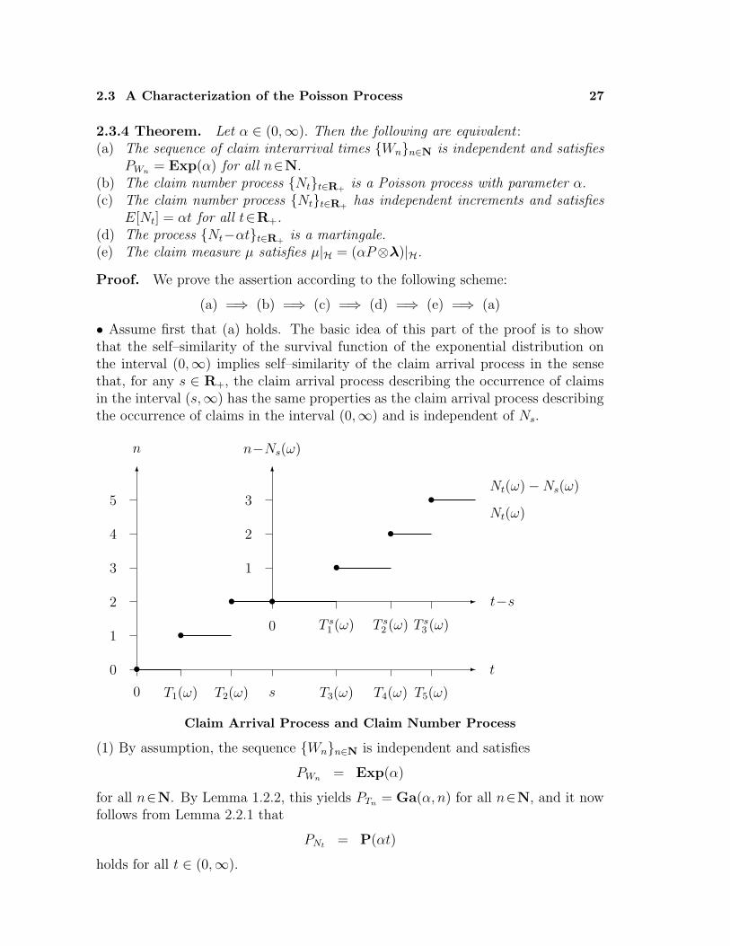
• Assume first that (a) holds. The basic idea of this part of the proof is to showthat the self–similarity of the survival function of the exponential distribution onthe interval (0,∞) implies self–similarity of the claim arrival process in the sensethat, for any s ∈ R+, the claim arrival process describing the occurrence of claimsin the interval (s,∞) has the same properties as the claim arrival process describingthe occurrence of claims in the interval (0,∞) and is independent of Ns.
0 -
1
2
3
4
5
n
-
1
2
3
n−Ns(ω)
6
0 T1(ω) T2(ω) s T3(ω) T4(ω) T5(ω)
t
6
0 T s1 (ω) T s
2 (ω) T s3 (ω)
t−s
•
•
• •
•
•
•Nt(ω)−Ns(ω)
Nt(ω)
Claim Arrival Process and Claim Number Process
(1) By assumption, the sequence Wnn∈N is independent and satisfies
PWn = Exp(α)
for all n∈N. By Lemma 1.2.2, this yields PTn = Ga(α, n) for all n∈N, and it nowfollows from Lemma 2.2.1 that
PNt = P(αt)
holds for all t ∈ (0,∞).
28 Chapter 2 The Claim Number Process
(2) Because of (1), we have
P [Nt = ∞] = 0
for all t ∈ R+, and it now follows from Lemma 2.1.4 that the probability of explosionis equal to zero. Thus, without loss of generality, we may and do assume thatNt(ω) < ∞ holds for all t ∈ R+ and all ω ∈ Ω, and this yields
Ω =∞∑
k=0
Nt = k
for all t ∈ R+.(3) For s ∈ R+, define
T s0 := 0
and, for all n ∈ N,
T sn :=
∞∑
k=0
(χNs=k · (Tk+n−s)
)
=∞∑
k=0
(χTk≤s<Tk+1 · (Tk+n−s)
).
Then the sequence T snn∈N0
satisfies T s0 = 0 and
T sn−1 < T s
n
for all n ∈ N. Therefore, T snn∈N0
is a claim arrival process. Let W snn∈N denote
the claim interarrival process induced by T snn∈N0
.(4) For each s ∈ R+, the finite dimensional distributions of the claim interarrivalprocesses W s
nn∈N and Wnn∈N are identical ; moreover, Ns and W snn∈N are
independent :Consider first t ∈ R+ and k ∈ N0. Then we have
Ns = k∩t < W s1 = Ns = k∩t < T s
1 = Ns = k∩t < Tk+1−s= Tk ≤ s < Tk+1∩s+t < Tk+1= Tk ≤ s∩s+t < Tk+1= Tk ≤ s∩s+t < Tk+Wk+1= Tk ≤ s∩s−Tk+t < Wk+1 .
Using the transformation formula for integrals, independence of Tk and Wk+1, andFubini’s theorem, we obtain
P [Ns = k∩t < W s1 ] = P [Tk ≤ s∩s−Tk+t < Wk+1]
2.3 A Characterization of the Poisson Process 29
=
∫
Ω
χTk≤s∩s−Tk+t<Wk+1(ω) dP (ω)
=
∫
R2
χ(−∞,s](r) χ(s−r+t,∞)(u) dPWk+1,Tk(u, r)
=
∫
R2
χ(−∞,s](r) χ(s−r+t,∞)(u) d(PWk+1⊗PTk
)(u, r)
=
∫
Rχ(−∞,s](r)
(∫
Rχ(s−r+t,∞)(u) dPWk+1
(u)
)dPTk
(r)
=
∫
(−∞,s]
(∫
Ω
χs−r+t<Wk+1(ω) dP (ω)
)dPTk
(r)
=
∫
(−∞,s]
P [s−r+t < Wk+1] dPTk(r) .
Using this formula twice together with the fact that the distribution of each Wn isExp(α) and hence memoryless on R+, we obtain
P [Ns = k∩t < W s1 ] =
∫
(−∞,s]
P [s−r+t < Wk+1] dPTk(r)
=
∫
(−∞,s]
P [s−r < Wk+1] P [t < Wk+1] dPTk(r)
=
∫
(−∞,s]
P [s−r < Wk+1] dPTk(r) · P [t < Wk+1]
= P [Ns = k∩0 < W s1 ] · P [t < Wk+1]
= P [Ns = k] · P [t < W1] .
Therefore, we have
P [Ns = k∩t < W s1 ] = P [Ns = k] · P [t < W1] .
Consider now n ∈ N, t1, . . . , tn ∈ R+, and k ∈ N0. For each j ∈ 2, . . . , n, we have
Ns = k∩tj < W sj = Ns = k∩tj < T s
j −T sj−1
= Ns = k∩tj < Tk+j−Tk+j−1= Ns = k∩tj < Wk+j .
Since the sequence Wnn∈N is independent and identically distributed, the previousidentities yield
P
[Ns = k ∩
n⋂j=1
tj < W sj
]
= P
[n⋂
j=1
(Ns = k∩tj < W s
j )]
30 Chapter 2 The Claim Number Process
= P
[(Ns = k∩t1 < W s
1 )∩
n⋂j=2
(Ns = k∩tj < W s
j )]
= P
[(Ns = k∩t1 < W s
1 )∩
n⋂j=2
(Ns = k∩tj < Wk+j
)]
= P
[(Ns = k∩t1 < W s
1 )∩
n⋂j=2
tj < Wk+j]
= P
[(Tk ≤ s∩s−Tk+t1 < Wk+1
)∩
n⋂j=2
tj < Wk+j]
= P [Tk ≤ s∩s−Tk+t1 < Wk+1] ·n∏
j=2
P [tj < Wk+j]
= P [Ns = k∩t1 < W s1 ] ·
n∏j=2
P [tj < Wk+j]
= P [Ns = k] · P [t1 < W1] ·n∏
j=2
P [tj < Wj]
= P [Ns = k] ·n∏
j=1
P [tj < Wj]
= P [Ns = k] · P[
n⋂j=1
tj < Wj]
.
Therefore, we have
P
[Ns = k ∩
n⋂j=1
tj < W sj
]= P [Ns = k] · P
[n⋂
j=1
tj < Wj]
.
Summation over k ∈ N0 yields
P
[n⋂
j=1
tj < W sj
]= P
[n⋂
j=1
tj < Wj]
.
Inserting this identity into the previous one, we obtain
P
[Ns = k ∩
n⋂j=1
tj < W sj
]= P [Ns = k] · P
[n⋂
j=1
tj < W sj
].
The last two identities show that the finite dimensional distributions of the claim in-terarrival processes W s
nn∈N and Wnn∈N are identical, and that Ns and W snn∈N
are independent. In particular, the sequence W snn∈N is independent and satisfies
PW sn
= Exp(α) for all n ∈ N.
2.3 A Characterization of the Poisson Process 31
(5) The identity PNs+h−Ns = PNhholds for all s, h ∈ R+ :
For all n ∈ N0, we have
Ns+h −Ns = n =∞∑
k=0
Ns = k∩Ns+h = k+n
=∞∑
k=0
Ns = k∩Tk+n ≤ s+h < Tk+n+1
=∞∑
k=0
Ns = k∩T sn ≤ h < T s
n+1
= T sn ≤ h < T s
n+1 .
Because of (4), the finite dimensional distributions of the claim interarrival processesW s
nn∈N and Wnn∈N are identical, and it follows that the finite dimensionaldistributions of the claim arrival processes T s
nn∈N0and Tnn∈N0
are identical aswell. This yields
P [Ns+h −Ns = n] = P [T sn ≤ h < T s
n+1]= P [Tn ≤ h < Tn+1]= P [Nh = n]
for all n ∈ N0.(6) The claim number process Ntt∈R+
has independent increments :Consider first s ∈ R+. Because of (4), Ns and W s
nn∈N are independent andthe finite dimensional distributions of the claim interarrival processes W s
nn∈Nand Wnn∈N are identical; consequently, Ns and T s
nn∈N0are independent and,
as noted before, the finite dimensional distributions of the claim arrival processesT s
nn∈N0and Tnn∈N0
are identical as well.Consider next s ∈ R+, m ∈ N, h1, . . . , hm ∈ R+, and k, k1, . . . , km ∈ N0. Then wehave
P
[Ns = k ∩
m⋂j=1
Ns+hj−Ns = kj
]
= P
[Ns = k ∩
m⋂j=1
T skj≤ hj < T s
kj+1]
= P [Ns = k] · P[
m⋂j=1
T skj≤ hj < T s
kj+1]
= P [Ns = k] · P[
m⋂j=1
Tkj≤ hj < Tkj+1
]
= P [Ns = k] · P[
m⋂j=1
Nhj= kj
].
32 Chapter 2 The Claim Number Process
We now claim that, for all m ∈ N, the identity
P
[m⋂
j=1
Ntj−Ntj−1= nj
]=
m∏j=1
P [Ntj−Ntj−1= nj] .
holds for all t0, t1, . . . , tm∈R+ such that 0 = t0 < t1 < . . . < tm, and n1, . . . , nm∈N0.This follows by induction:The assertion is obvious for m = 1.Assume now that it holds for some m ∈ N and consider t0, t1, . . . , tm, tm+1 ∈ R+
such that 0 = t0 < t1 < . . . < tm < tm+1, and n1, . . . , nm, nm+1 ∈ N0. Forj ∈ 0, 1, . . . ,m, define hj := tj+1−t1. Then we have 0 = h0 < h1 < . . . < hm andhence, by assumption and because of (5),
P
[m⋂
j=1
Nhj−Nhj−1
= nj+1]
=m∏
j=1
P [Nhj−Nhj−1
= nj+1]
=m∏
j=1
P [Nhj−hj−1= nj+1]
=m∏
j=1
P [Ntj+1−tj = nj+1]
=m∏
j=1
P [Ntj+1−Ntj = nj+1]
=m+1∏j=2
P [Ntj−Ntj−1= nj] .
Using the identity established before with s := t1, this yields
P
[m+1⋂j=1
Ntj−Ntj−1= nj
]= P
[m+1⋂j=1
Ntj =
j∑i=1
ni
]
= P
[Nt1 = n1 ∩
m+1⋂j=2
Ntj =
j∑i=1
ni
]
= P
[Nt1 = n1 ∩
m+1⋂j=2
Ntj−Nt1 =
j∑i=2
ni
]
= P
[Nt1 = n1 ∩
m⋂j=1
Ntj+1
−Nt1 =
j+1∑i=2
ni
]
= P
[Nt1 = n1 ∩
m⋂j=1
Nt1+hj
−Nt1 =
j+1∑i=2
ni
]
2.3 A Characterization of the Poisson Process 33
= P [Nt1 = n1] · P[
m⋂j=1
Nhj
=
j+1∑i=2
ni
]
= P [Nt1 = n1] · P[
m⋂j=1
Nhj−Nhj−1
= nj+1]
= P [Nt1 = n1] ·m+1∏j=2
P [Ntj−Ntj−1= nj]
=m+1∏j=1
P [Ntj−Ntj−1= nj] ,
which is the assertion for m+1. This proves our claim, and it follows that the claimnumber process Ntt∈R+
has independent increments.(7) It now follows from (6), (5), and (1) that the claim number process Ntt∈R+
isa Poisson process with parameter α. Therefore, (a) implies (b).• Assume now that (b) holds. Since Ntt∈R+
is a Poisson process with parameter α,it is clear that Ntt∈R+
has independent increments and satisfies E[Nt] = αt forall t ∈ R+. Therefore, (b) implies (c).
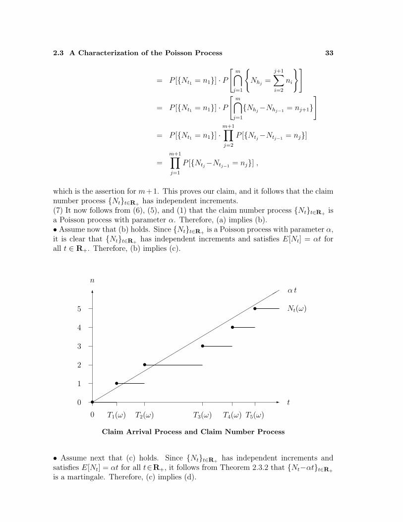
6
0 T1(ω) T2(ω) T3(ω) T4(ω) T5(ω)
n
0 -
1
2
3
4
5
t""
""
""
""
""
""
""
""
""
""
""
""
""
""" α t
•
•
•
•
•
• Nt(ω)
Claim Arrival Process and Claim Number Process
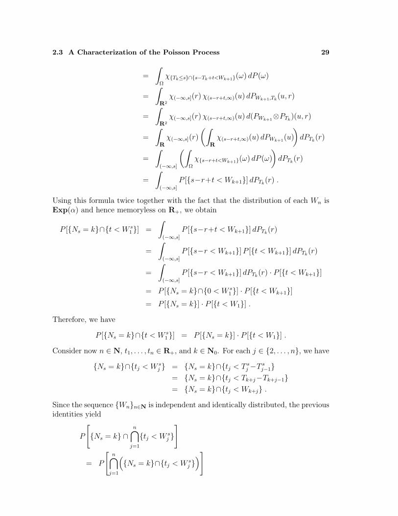
• Assume next that (c) holds. Since Ntt∈R+has independent increments and
satisfies E[Nt] = αt for all t∈R+, it follows from Theorem 2.3.2 that Nt−αtt∈R+
is a martingale. Therefore, (c) implies (d).
34 Chapter 2 The Claim Number Process
• Assume now that (d) holds. For all s, t ∈ R+ such that s ≤ t and for all A ∈ Fs,Lemma 2.1.6 together with the martingale property of Nr−αrr∈R+
yields
µ[A×(s, t]] =
∫
A
(Nt−Ns) dP
=
∫
A
α(t−s) dP
= α(t−s) · P [A]
= α λ[(s, t]] · P [A]
= (αP⊗λ)[A×(s, t]] .
Since A×(s, t] is a typical set of E , this gives
µ|E = (αP⊗λ)|E .
Since Ω×(0,∞) =∑∞
n=1 Ω×(n−1, n], the set Ω×(0,∞) is the union of countablymany sets in E such that αP ⊗λ is finite on each of these sets. This means thatthe measure µ|E = (αP⊗λ)|E is σ–finite. Furthermore, since the family Fss∈R+
is increasing, it is easy to see that E is stable under intersection. Since σ(E) = H,it now follows from the uniqueness theorem for σ–finite measures that
µ|H = (αP⊗λ)|H .
Therefore, (d) implies (e)• Assume finally that (e) holds. In order to determine the finite dimensional distri-butions of the claim interarrival process Wnn∈N, we have to study the probabilityof events having the form
A ∩ t < Wnfor n ∈ N, t ∈ R+, and A ∈ σ(Wkk∈1,...,n−1) = σ(Tkk∈0,1,...,n−1).(1) For n ∈ N0, define
En :=
n⋂
k=1
tk < Tk∣∣∣∣∣t1, . . . , tn ∈ R+
.
Since En is stable under intersection and satisfies σ(En) = σ(Tkk∈0,1,...,n), it issufficient to study the probability of events having the form
A ∩ t < Wnfor n ∈ N, t ∈ R+, and A ∈ En−1.(2) For n ∈ N, t ∈ R+, and A ∈ En−1, define
Hn,t(A) :=(ω, u) | ω ∈ A, Tn−1(ω)+t < u ≤ Tn(ω)
.
2.3 A Characterization of the Poisson Process 35
Then we have
U−1n (Hn,t(A)) = A ∩ Tn−1+t < Tn
= A ∩ t < Wn ,
as well as
U−1k (Hn,t(A)) = ∅
for all k ∈ N such that k 6= n. This gives
A ∩ t < Wn =∞∑
k=1
U−1k (Hn,t(A)) .
Now the problem is to show that Hn,t(A) ∈ H; if this is true, then we can apply theassumption on the claim measure µ in order to compute P [A ∩ t < Wn].(3) The relation Hn,t(A) ∈ H holds for all n ∈ N, t ∈ R+, and A ∈ En−1:First, for all k, m ∈ N0 such that k ≤ m and all p, q, s, t ∈ R+ such that s+t < p < q,we have(
s < Tk∩Tm+t ≤ p)× (p, q] =
(Ns < k∩m ≤ Np−t
)× (p, q] ,
which is a set in E and hence in H.Next, for all k, m ∈ N such that k ≤ m and all s, t ∈ R+, define
Hk,m;s,t := (ω, u) | s < Tk(ω), Tm(ω)+t < u .
Then we have
Hk,m;s,t =⋃
p,q∈Q, s+t<p<q
(s < Tk∩Tm+t ≤ p
)× (p, q] ,
and hence Hk,m;s,t ∈ H.Finally, since
A =n−1⋂
k=1
tk < Tk
for suitable t1, . . . , tn−1 ∈ R+, we have
Hn,t(A) = Hn,t
(n−1⋂
k=1
tk < Tk)
=
(ω, u)
∣∣∣∣∣ ω ∈n−1⋂
k=1
tk < Tk, Tn−1(ω)+t < u ≤ Tn(ω)
=n−1⋂
k=1
(ω, u) | tk < Tk(ω), Tn−1(ω)+t < u ∩ (ω, u) | Tn(ω) < u
=n−1⋂
k=1
Hk,n−1;tk,t ∩Hn,n;0,0 ,
and hence Hn,t(A) ∈ H.

36 Chapter 2 The Claim Number Process
(4) Consider n ∈ N, t ∈ R+, and A ∈ En−1. Because of (2) and (3), the assumptionon the claim measure yields
P [A ∩ t < Wn] = P
[ ∞∑
k=1
U−1k (Hn,t(A))
]
=∞∑
k=1
P [U−1k (Hn,t(A))]
=∞∑
k=1
PUk[Hn,t(A)]
= µ[Hn,t(A)]
= (αP⊗λ)[Hn,t(A)] .
Thus, using the fact that the Lebesgue measure is translation invariant and vanisheson singletons, we have
∫
Rχ(Tn−1(ω)+t,Tn(ω)](s) dλ(s) =
∫
Rχ[t,Wn(ω))(s) dλ(s)
hence
1
αP [A ∩t < Wn] = (P⊗λ)[Hn,t(A)]
=
∫
Ω×RχHn,t(A)(ω, s) d(P⊗λ)(ω, s)
=
∫
Ω×RχA(ω) χ(Tn−1(ω)+t,Tn(ω)](s) d(P⊗λ)(ω, s)
=
∫
Ω
χA(ω)
(∫
Rχ(Tn−1(ω)+t,Tn(ω)](s) dλ(s)
)dP (ω)
=
∫
Ω
χA(ω)
(∫
Rχ[t,Wn(ω))(s) dλ(s)
)dP (ω)
=
∫
Ω×RχA(ω) χ[t,Wn(ω))(s) d(P⊗λ)(ω, s)
=
∫
Ω×Rχ[t,∞)(s) χA∩s<Wn(ω) d(P⊗λ)(ω, s)
=
∫
Rχ[t,∞)(s)
(∫
Ω
χA∩s<Wn dP (ω)
)dλ(s)
=
∫
[t,∞)
P [A ∩s < Wn] dλ(s) ,
and thus
P [A ∩ t < Wn] = α
∫
[t,∞)
P [A ∩s < Wn] dλ(s) .
2.3 A Characterization of the Poisson Process 37
(5) Consider n ∈ N and A ∈ En−1. Then the function g : R → R, given by
g(t) :=
0 if t ∈ (−∞, 0)
P [A ∩t < Wn] if t ∈ R+ ,
is bounded; moreover, g is monotone decreasing on R+ and hence almost surelycontinuous. This implies that g is Riemann integrable and satisfies
∫
[0,t)
g(s) dλ(s) =
∫ t
0
g(s) ds
for all t ∈ R+. Because of (4), the restriction of g to R+ satisfies
g(t) = P [A ∩t < Wn]
= α
∫
[t,∞)
P [A ∩s < Wn] dλ(s)
= α
∫
[t,∞)
g(s) dλ(s) ,
and thus
g(t)− g(0) = −α
∫
[0,t)
g(s) dλ(s)
= −α
∫ t
0
g(s) ds .
This implies that the restriction of g to R+ is differentiable and satisfies the differ-ential equation
g′(t) = −α g(t)
with initial condition g(0) = P [A].For all t ∈ R+, this yields
g(t) = P [A] · e−αt ,
and thus
P [A ∩t < Wn] = g(t)
= P [A] · e−αt .
(6) Consider n ∈ N. Since Ω ∈ En−1, the previous identity yields
P [t < Wn] = e−αt
for all t ∈ R+. Inserting this identity into the previous one, we obtain
P [A ∩t < Wn] = P [A] · P [t < Wn]for all t ∈ R+ and A ∈ En−1. This shows that σ(W1, . . . ,Wn−1) and σ(Wn) areindependent.
38 Chapter 2 The Claim Number Process
(7) Because of (6), it follows by induction that the sequence Wnn∈N is independentand satisfies
PWn = Exp(α)
for all n ∈ N. Therefore, (e) implies (a). 2
To conclude this section, let us consider the prediction problem for claim numberprocesses having independent increments and finite second moments:
2.3.5 Theorem (Prediction). Assume that the claim number process Ntt∈R+
has independent increments and finite second moments. Then the inequality
E[(Nt−(Ns+E[Nt−Ns]))2] ≤ E[(Nt−Z)2]
holds for all s, t ∈ R+ such that s ≤ t and for every random variable Z satisfyingE[Z2] < ∞ and σ(Z) ⊆ Fs.
Proof. Define Z0 := Ns + E[Nt−Ns]. By assumption, the pair Nt−Z0, Z0−Zis independent, and this yields
E[(Nt−Z0)(Z0−Z)] = E[Nt−Z0] · E[Z0−Z]
= E[Nt−(Ns+E[Nt−Ns])] · E[Z0−Z]
= 0 .
Therefore, we have
E[(Nt−Z)2] = E[((Nt−Z0) + (Z0−Z))2]
= E[(Nt−Z0)2] + E[(Z0−Z)2] .
The last expression attains its minimum for Z := Z0. 2
Thus, for a claim number process having independent increments and finite secondmoments, the best prediction under expected squared error loss of Nt by a randomvariable depending only on the history of the claim number process up to time s isgiven by Ns + E[Nt−Ns].
As an immediate consequence of the previous result, we have the following:
2.3.6 Corollary (Prediction). Assume that the claim number process Ntt∈R+
is a Poisson process with parameter α. Then the inequality
E[(Nt−(Ns+α(t−s)))2] ≤ E[(Nt−Z)2]
holds for all s, t ∈ R+ such that s ≤ t and for every random variable Z satisfyingE[Z2] < ∞ and σ(Z) ⊆ Fs.
As in the case of Corollary 2.3.3, the previous result can be considerably improved:
2.3 A Characterization of the Poisson Process 39
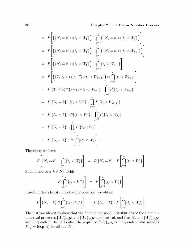
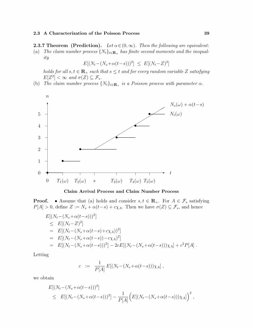
2.3.7 Theorem (Prediction). Let α∈(0,∞). Then the following are equivalent :(a) The claim number process Ntt∈R+
has finite second moments and the inequal-ity
E[(Nt−(Ns+α(t−s)))2] ≤ E[(Nt−Z)2]
holds for all s, t ∈ R+ such that s ≤ t and for every random variable Z satisfyingE[Z2] < ∞ and σ(Z) ⊆ Fs.
(b) The claim number process Ntt∈R+is a Poisson process with parameter α.
6
0 T1(ω) T2(ω) s T3(ω) T4(ω) T5(ω)
n
0 -
1
2
3
4
5
t
""
""
""
""
""
""
""
""
""Ns(ω) + α(t−s)
•
•
•
•
•
• Nt(ω)
Claim Arrival Process and Claim Number Process
Proof. • Assume that (a) holds and consider s, t ∈ R+. For A ∈ Fs satisfyingP [A] > 0, define Z := Ns + α(t−s) + cχA. Then we have σ(Z) ⊆ Fs, and hence
E[(Nt−(Ns+α(t−s)))2]
≤ E[(Nt−Z)2]
= E[(Nt−(Ns+α(t−s)+cχA))2]
= E[(Nt−(Ns+α(t−s))−cχA)2]
= E[(Nt−(Ns+α(t−s)))2]− 2cE[(Nt−(Ns+α(t−s)))χA] + c2P [A] .
Letting
c :=1
P [A]E[(Nt−(Ns+α(t−s)))χA] ,
we obtain
E[(Nt−(Ns+α(t−s)))2]
≤ E[(Nt−(Ns+α(t−s)))2]− 1
P [A]
(E[(Nt−(Ns+α(t−s)))χA]
)2
,
40 Chapter 2 The Claim Number Process
hence
E[(Nt−(Ns+α(t−s)))χA] = 0 ,
and thus ∫
A
((Nt−αt
)− (Ns−αs
))dP =
∫
A
(Nt − (Ns+α(t−s))
)dP
= 0 .
Of course, the previous identity is also valid for A ∈ Fs satisfying P [A] = 0.This shows that the process Nt−αtt∈R+
is a martingale, and it now follows fromTheorem 2.3.4 that the claim number process Ntt∈R+
is a Poisson process withparameter α. Therefore, (a) implies (b).• The converse implication is obvious from Corollary 2.3.6. 2
Problems2.3.A Discrete Time Model: Adopt the definitions given in this section to the dis-
crete time model. The claim number process Nll∈N0is a binomial process
or Bernoulli process with parameter ϑ ∈ (0, 1) if it has stationary independentincrements such that PNl
= B(l, ϑ) holds for all l ∈ N.
2.3.B Discrete Time Model: Assume that the claim number process Nll∈N0has in-
dependent increments. Then the centered claim number process Nl−E[Nl]l∈N0
is a martingale.
2.3.C Discrete Time Model: Let ϑ ∈ (0, 1). Then the following are equivalent:(a) The claim number process Nll∈N0
satisfies
PNl= B(l, ϑ)
for all l ∈ N as well as
P
m⋂
j=1
Nj−Nj−1 = kj∣∣∣∣∣∣Nm = n
=
(m
n
)−1
for all m∈N and for all n∈N0 and k1, . . . , km∈0, 1 such that∑m
j=1 kj = n.(b) The claim number process Nll∈N0
satisfies
PNl= B(l, ϑ)
for all l ∈ N as well as
P
m⋂
j=1
Nlj−Nlj−1 = kj∣∣∣∣∣∣Nlm = n
=
m∏
j=1
(lj − lj−1
kj
)·(
lmn
)−1
for all m ∈ N and l0, l1, . . . , lm ∈ N0 such that 0 = l0 < l1 < . . . < lmand for all n ∈ N0 and k1, . . . , km ∈ N0 such that kj ≤ lj − lj−1 for allj ∈ 1, . . . ,m and
∑mj=1 kj = n.
(c) The claim number process Nll∈N0is a binomial process with parameter ϑ.
2.4 Remarks 41
2.3.D Discrete Time Model: Let ϑ ∈ (0, 1). Then the following are equivalent:(a) The sequence of claim interarrival times Wnn∈N is independent and satis-
fies PWn = Geo(ϑ) for all n ∈ N.(b) The claim number process Nll∈N0
is a binomial process with parameter ϑ.(c) The claim number process Nll∈N0
has independent increments and satis-fies E[Nl] = ϑl for all l ∈ N0.
(d) The process Nl−ϑll∈N0is a martingale.
Hint : Prove that (a) ⇐⇒ (b) ⇐⇒ (c) ⇐⇒ (d).
2.3.E Discrete Time Model: Assume that the claim number process Nll∈N0has
independent increments. Then the inequality
E[(Nm−(Nl+E[Nm−Nl]))2] ≤ E[(Nl−Z)2]
holds for all l, m ∈ N0 such that l ≤ m and for every random variable Z satisfyingσ(Z) ⊆ Fl.
2.3.F Discrete Time Model: Let ϑ ∈ (0, 1). Then the following are equivalent:(a) The inequality
E[(Nm−(Nl+ϑ(m−l)))2] ≤ E[(Nm−Z)2]
holds for all l, m ∈ N0 such that l ≤ m and for every random variable Zsatisfying σ(Z) ⊆ Fl.
(b) The claim number process Nll∈N0is a binomial process with parameter ϑ.
2.3.G Multiple Life Insurance: Adopt the definitions given in this section to multiplelife insurance. Study stationarity and independence of the increments of theprocess Ntt∈R+
as well as the martingale property of Nt−E[Nt]t∈R+.
2.3.H Single Life Insurance:(a) The process Ntt∈R+
does not have stationary increments.(b) The process Ntt∈R+
has independent increments if and only if the distri-bution of T is degenerate.
(c) The process Nt−E[Nt]t∈R+is a martingale if and only if the distribution
of T is degenerate.
2.4 Remarks
The definition of the increments of the claim number process suggests to define, foreach ω ∈ Ω and all B ∈ B(R),
N(ω)(B) :=∞∑
n=1
χTn∈B(ω) .
Then, for each ω ∈ Ω, the map N(ω) : B(R) → N0∪∞ is a measure, which is σ–finite whenever the probability of explosion is equal to zero. This point of view leadsto the theory of point processes ; see Kerstan, Matthes, and Mecke [1974], Grandell
42 Chapter 2 The Claim Number Process
[1977], Neveu [1977], Matthes, Kerstan, and Mecke [1978], Cox and Isham [1980],Bremaud [1981], Kallenberg [1983], Karr [1991], Konig and Schmidt [1992], Kingman[1993], and Reiss [1993]; see also Mathar and Pfeifer [1990] for an introduction intothe subject.
The implication (a) =⇒ (b) of Theorem 2.3.4 can be used to show that the Poissonprocess does exist: Indeed, Kolmogorov’s existence theorem asserts that, for anysequence Qnn∈N of probability measures B(R) → [0, 1], there exists a probabilityspace (Ω,F , P ) and a sequence Wnn∈N of random variables Ω → R such that thesequence Wnn∈N is independent and satisfies PWn = Qn for all n ∈ N. LettingTn :=
∑nk=1 Wk for all n ∈ N0 and Nt :=
∑∞n=1 χTn≤t for all t ∈ R+, we obtain a
claim arrival process Tnn∈N0and a claim number process Ntt∈R+
. In particular,if Qn = Exp(α) holds for all n ∈ N, then it follows from Theorem 2.3.4 thatNtt∈R+
is a Poisson process with parameter α. The implication (d) =⇒ (b) ofTheorem 2.3.4 is due to Watanabe [1964]. The proof of the implications (d) =⇒ (e)and (e) =⇒ (a) of Theorem 2.3.4 follows Letta [1984].
Theorems 2.3.2 and 2.3.4 are typical examples for the presence of martingales incanonical situations in risk theory; see also Chapter 7 below.
In the case where the claim interarrival times are independent and identically (butnot necessarily exponentially) distributed, the claim arrival process or, equivalently,the claim number process is said to be a renewal process ; see e. g. Gut [1988],Alsmeyer [1991], Grandell [1991], and Resnick [1992]. This case will be considered,to a limited extent, in Chapter 7 below.
The case where the claim interarrival times are independent and exponentially (butnot necessarily identically) distributed will be studied in Section 3.4 below.
We shall return to the Poisson process at various places in this book: The Poissonprocess occurs as a very special case in the rather analytical theory of regular claimnumber processes satisfying the Chapman–Kolmogorov equations, which will bedeveloped in Chapter 3, and it also occurs as a degenerate case in the class ofmixed Poisson processes, which will be studied in Chapter 4. Moreover, thinning,decomposition, and superposition of Poisson processes, which are important withregard to reinsurance, will be discussed in Chapters 5 and 6.
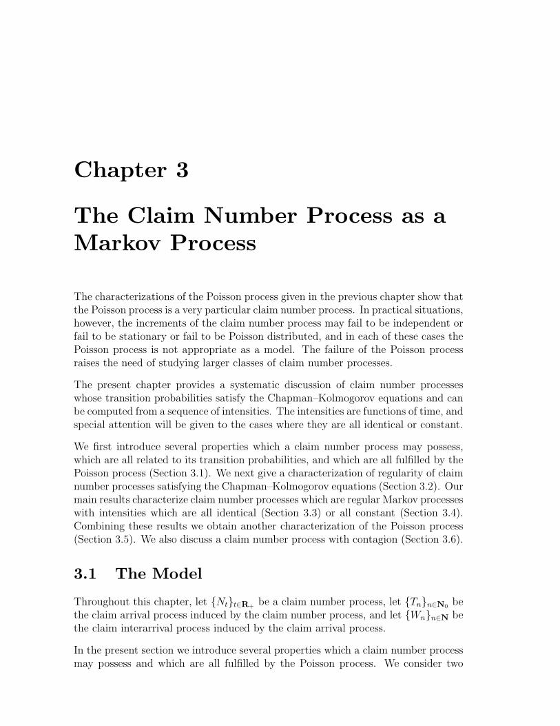
Chapter 3
The Claim Number Process as aMarkov Process
The characterizations of the Poisson process given in the previous chapter show thatthe Poisson process is a very particular claim number process. In practical situations,however, the increments of the claim number process may fail to be independent orfail to be stationary or fail to be Poisson distributed, and in each of these cases thePoisson process is not appropriate as a model. The failure of the Poisson processraises the need of studying larger classes of claim number processes.
The present chapter provides a systematic discussion of claim number processeswhose transition probabilities satisfy the Chapman–Kolmogorov equations and canbe computed from a sequence of intensities. The intensities are functions of time, andspecial attention will be given to the cases where they are all identical or constant.
We first introduce several properties which a claim number process may possess,which are all related to its transition probabilities, and which are all fulfilled by thePoisson process (Section 3.1). We next give a characterization of regularity of claimnumber processes satisfying the Chapman–Kolmogorov equations (Section 3.2). Ourmain results characterize claim number processes which are regular Markov processeswith intensities which are all identical (Section 3.3) or all constant (Section 3.4).Combining these results we obtain another characterization of the Poisson process(Section 3.5). We also discuss a claim number process with contagion (Section 3.6).
3.1 The Model
Throughout this chapter, let Ntt∈R+be a claim number process, let Tnn∈N0
bethe claim arrival process induced by the claim number process, and let Wnn∈N bethe claim interarrival process induced by the claim arrival process.
In the present section we introduce several properties which a claim number processmay possess and which are all fulfilled by the Poisson process. We consider two
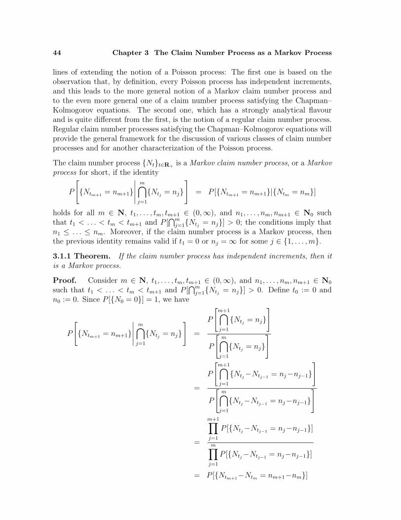
44 Chapter 3 The Claim Number Process as a Markov Process
lines of extending the notion of a Poisson process: The first one is based on theobservation that, by definition, every Poisson process has independent increments,and this leads to the more general notion of a Markov claim number process andto the even more general one of a claim number process satisfying the Chapman–Kolmogorov equations. The second one, which has a strongly analytical flavourand is quite different from the first, is the notion of a regular claim number process.Regular claim number processes satisfying the Chapman–Kolmogorov equations willprovide the general framework for the discussion of various classes of claim numberprocesses and for another characterization of the Poisson process.
The claim number process Ntt∈R+is a Markov claim number process, or a Markov
process for short, if the identity
P
[Ntm+1 = nm+1
∣∣∣∣∣m⋂
j=1
Ntj = nj]
= P [Ntm+1 = nm+1|Ntm = nm]
holds for all m ∈ N, t1, . . . , tm, tm+1 ∈ (0,∞), and n1, . . . , nm, nm+1 ∈ N0 suchthat t1 < . . . < tm < tm+1 and P [
⋂mj=1Ntj = nj] > 0; the conditions imply that
n1 ≤ . . . ≤ nm. Moreover, if the claim number process is a Markov process, thenthe previous identity remains valid if t1 = 0 or nj = ∞ for some j ∈ 1, . . . ,m.3.1.1 Theorem. If the claim number process has independent increments, then itis a Markov process.
Proof. Consider m ∈ N, t1, . . . , tm, tm+1 ∈ (0,∞), and n1, . . . , nm, nm+1 ∈ N0
such that t1 < . . . < tm < tm+1 and P [⋂m
j=1Ntj = nj] > 0. Define t0 := 0 andn0 := 0. Since P [N0 = 0] = 1, we have
P
[Ntm+1 = nm+1
∣∣∣∣∣m⋂
j=1
Ntj = nj]
=
P
[m+1⋂j=1
Ntj = nj]
P
[m⋂
j=1
Ntj = nj]
=
P
[m+1⋂j=1
Ntj−Ntj−1= nj−nj−1
]
P
[m⋂
j=1
Ntj−Ntj−1= nj−nj−1
]
=
m+1∏j=1
P [Ntj−Ntj−1= nj−nj−1]
m∏j=1
P [Ntj−Ntj−1= nj−nj−1]
= P [Ntm+1−Ntm = nm+1−nm]
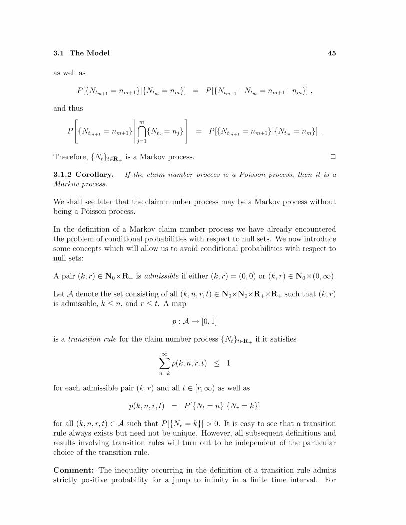
3.1 The Model 45
as well as
P [Ntm+1 = nm+1|Ntm = nm] = P [Ntm+1−Ntm = nm+1−nm] ,
and thus
P
[Ntm+1 = nm+1
∣∣∣∣∣m⋂
j=1
Ntj = nj]
= P [Ntm+1 = nm+1|Ntm = nm] .
Therefore, Ntt∈R+is a Markov process. 2
3.1.2 Corollary. If the claim number process is a Poisson process, then it is aMarkov process.
We shall see later that the claim number process may be a Markov process withoutbeing a Poisson process.
In the definition of a Markov claim number process we have already encounteredthe problem of conditional probabilities with respect to null sets. We now introducesome concepts which will allow us to avoid conditional probabilities with respect tonull sets:
A pair (k, r) ∈ N0×R+ is admissible if either (k, r) = (0, 0) or (k, r) ∈ N0×(0,∞).
Let A denote the set consisting of all (k, n, r, t) ∈ N0×N0×R+×R+ such that (k, r)is admissible, k ≤ n, and r ≤ t. A map
p : A → [0, 1]
is a transition rule for the claim number process Ntt∈R+if it satisfies
∞∑
n=k
p(k, n, r, t) ≤ 1
for each admissible pair (k, r) and all t ∈ [r,∞) as well as
p(k, n, r, t) = P [Nt = n|Nr = k]
for all (k, n, r, t) ∈ A such that P [Nr = k] > 0. It is easy to see that a transitionrule always exists but need not be unique. However, all subsequent definitions andresults involving transition rules will turn out to be independent of the particularchoice of the transition rule.
Comment: The inequality occurring in the definition of a transition rule admitsstrictly positive probability for a jump to infinity in a finite time interval. For
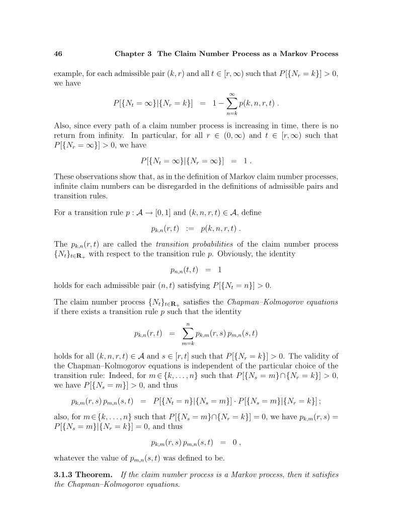
46 Chapter 3 The Claim Number Process as a Markov Process
example, for each admissible pair (k, r) and all t ∈ [r,∞) such that P [Nr = k] > 0,we have
P [Nt = ∞|Nr = k] = 1−∞∑
n=k
p(k, n, r, t) .
Also, since every path of a claim number process is increasing in time, there is noreturn from infinity. In particular, for all r ∈ (0,∞) and t ∈ [r,∞) such thatP [Nr = ∞] > 0, we have
P [Nt = ∞|Nr = ∞] = 1 .
These observations show that, as in the definition of Markov claim number processes,infinite claim numbers can be disregarded in the definitions of admissible pairs andtransition rules.
For a transition rule p : A → [0, 1] and (k, n, r, t) ∈ A, define
pk,n(r, t) := p(k, n, r, t) .
The pk,n(r, t) are called the transition probabilities of the claim number processNtt∈R+
with respect to the transition rule p. Obviously, the identity
pn,n(t, t) = 1
holds for each admissible pair (n, t) satisfying P [Nt = n] > 0.
The claim number process Ntt∈R+satisfies the Chapman–Kolmogorov equations
if there exists a transition rule p such that the identity
pk,n(r, t) =n∑
m=k
pk,m(r, s) pm,n(s, t)
holds for all (k, n, r, t) ∈ A and s ∈ [r, t] such that P [Nr = k] > 0. The validity ofthe Chapman–Kolmogorov equations is independent of the particular choice of thetransition rule: Indeed, for m∈k, . . . , n such that P [Ns = m∩Nr = k] > 0,we have P [Ns = m] > 0, and thus
pk,m(r, s) pm,n(s, t) = P [Nt = n|Ns = m] · P [Ns = m|Nr = k] ;also, for m∈k, . . . , n such that P [Ns = m∩Nr = k] = 0, we have pk,m(r, s) =P [Ns = m|Nr = k] = 0, and thus
pk,m(r, s) pm,n(s, t) = 0 ,
whatever the value of pm,n(s, t) was defined to be.
3.1.3 Theorem. If the claim number process is a Markov process, then it satisfiesthe Chapman–Kolmogorov equations.
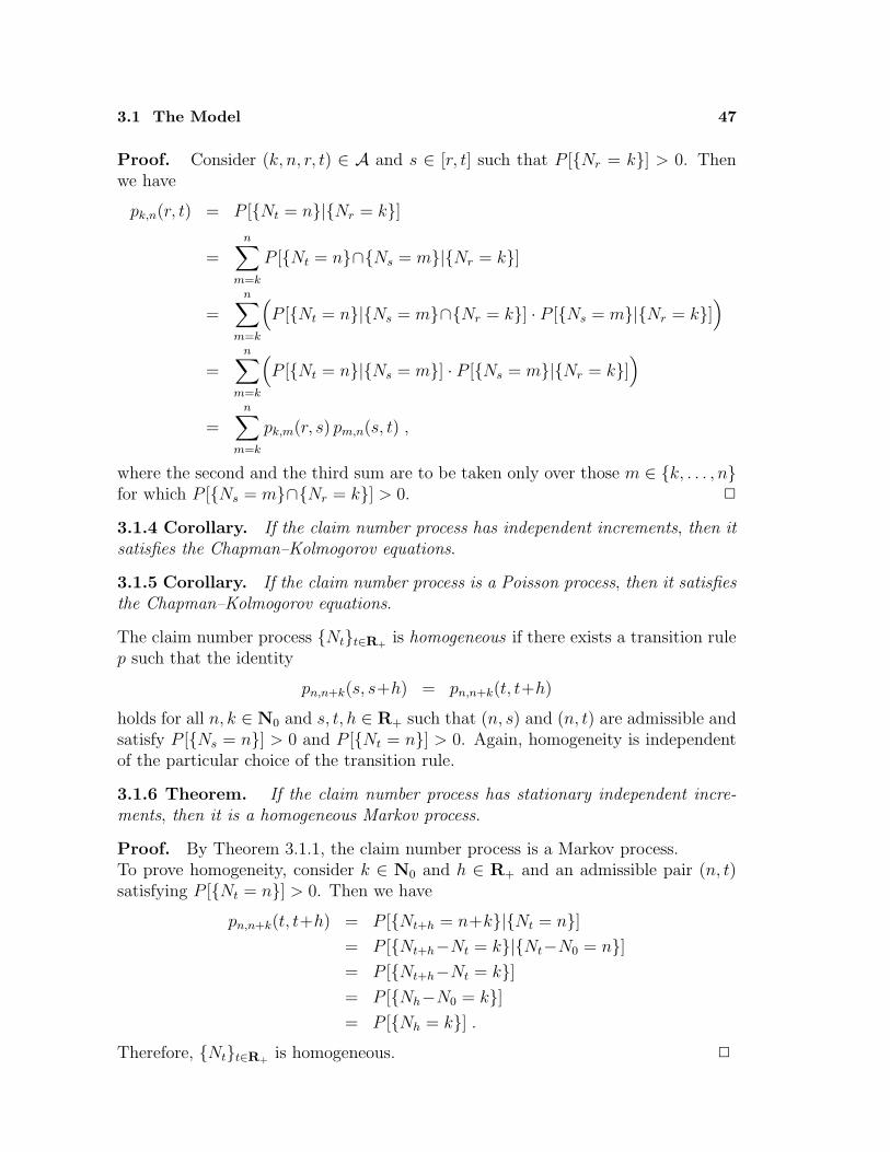
3.1 The Model 47
Proof. Consider (k, n, r, t) ∈ A and s ∈ [r, t] such that P [Nr = k] > 0. Thenwe have
pk,n(r, t) = P [Nt = n|Nr = k]
=n∑
m=k
P [Nt = n∩Ns = m|Nr = k]
=n∑
m=k
(P [Nt = n|Ns = m∩Nr = k] · P [Ns = m|Nr = k]
)
=n∑
m=k
(P [Nt = n|Ns = m] · P [Ns = m|Nr = k]
)
=n∑
m=k
pk,m(r, s) pm,n(s, t) ,
where the second and the third sum are to be taken only over those m ∈ k, . . . , nfor which P [Ns = m∩Nr = k] > 0. 2
3.1.4 Corollary. If the claim number process has independent increments, then itsatisfies the Chapman–Kolmogorov equations.
3.1.5 Corollary. If the claim number process is a Poisson process, then it satisfiesthe Chapman–Kolmogorov equations.
The claim number process Ntt∈R+is homogeneous if there exists a transition rule
p such that the identity
pn,n+k(s, s+h) = pn,n+k(t, t+h)
holds for all n, k ∈ N0 and s, t, h ∈ R+ such that (n, s) and (n, t) are admissible andsatisfy P [Ns = n] > 0 and P [Nt = n] > 0. Again, homogeneity is independentof the particular choice of the transition rule.
3.1.6 Theorem. If the claim number process has stationary independent incre-ments, then it is a homogeneous Markov process.
Proof. By Theorem 3.1.1, the claim number process is a Markov process.To prove homogeneity, consider k ∈ N0 and h ∈ R+ and an admissible pair (n, t)satisfying P [Nt = n] > 0. Then we have
pn,n+k(t, t+h) = P [Nt+h = n+k|Nt = n]= P [Nt+h−Nt = k|Nt−N0 = n]= P [Nt+h−Nt = k]= P [Nh−N0 = k]= P [Nh = k] .
Therefore, Ntt∈R+is homogeneous. 2
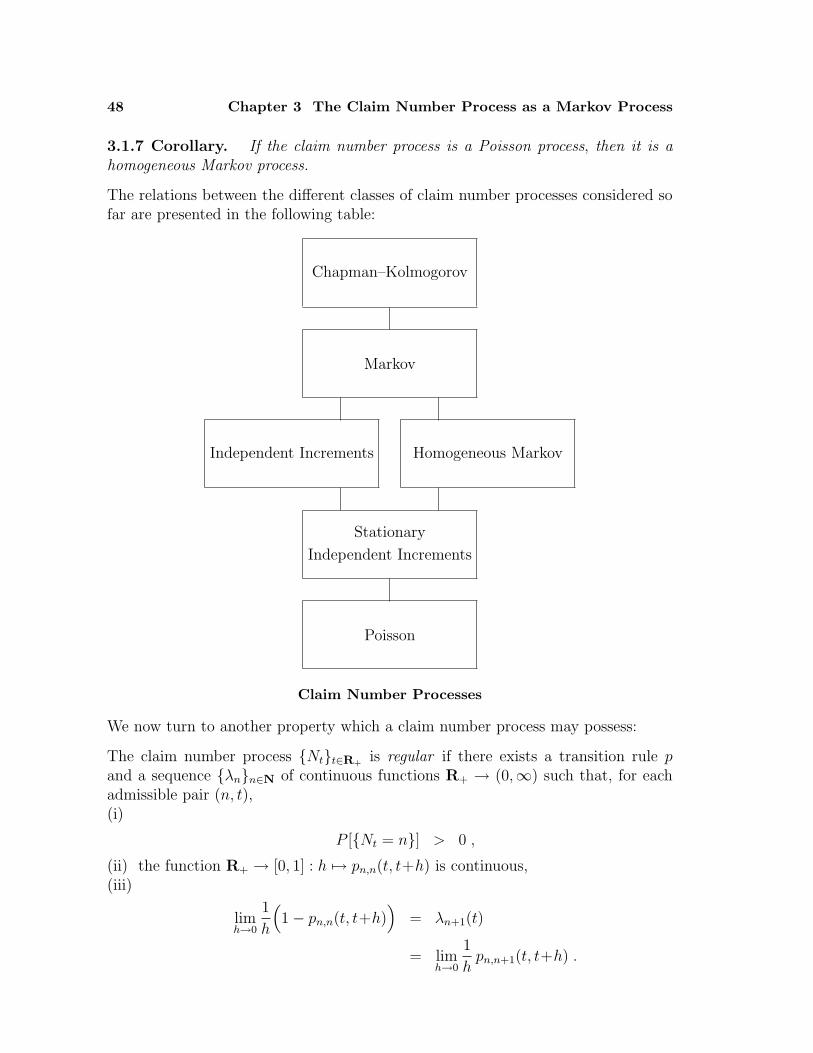
48 Chapter 3 The Claim Number Process as a Markov Process
3.1.7 Corollary. If the claim number process is a Poisson process, then it is ahomogeneous Markov process.
The relations between the different classes of claim number processes considered sofar are presented in the following table:
Chapman–Kolmogorov
Markov
Independent Increments Homogeneous Markov
Stationary
Independent Increments
Poisson
Claim Number Processes
We now turn to another property which a claim number process may possess:
The claim number process Ntt∈R+is regular if there exists a transition rule p
and a sequence λnn∈N of continuous functions R+ → (0,∞) such that, for eachadmissible pair (n, t),(i)
P [Nt = n] > 0 ,
(ii) the function R+ → [0, 1] : h 7→ pn,n(t, t+h) is continuous,(iii)
limh→0
1
h
(1− pn,n(t, t+h)
)= λn+1(t)
= limh→0
1
hpn,n+1(t, t+h) .
3.1 The Model 49
In this case, λnn∈N is said to be the sequence of intensities of the claim numberprocess. Because of (i), regularity is independent of the particular choice of thetransition rule.
Comment:– Condition (i) means that at any time t ∈ (0,∞) every finite number of claims is
attained with strictly positive probability.– Condition (ii) means that, conditionally on the event Nt = n, the probability of
no jumps in a finite time interval varies smoothly with the length of the interval.– Condition (iii) means that, conditionally on the event Nt = n, the tendency for
a jump of any height is, in an infinitesimal time interval, equal to the tendencyfor a jump of height one.
3.1.8 Theorem. If the claim number process is a Poisson process with para-meter α, then it is a homogeneous regular Markov process with intensities λnn∈Nsatisfying λn(t) = α for all n∈N and t∈R+.
Proof. By Corollary 3.1.7, the claim number process is a homogeneous Markovprocess.To prove the assertion on regularity, consider an admissible pair (n, t).First, since
P [Nt = n] = e−αt (αt)n
n!,
we have P [Nt = n] > 0, which proves (i).Second, since
pn,n(t, t+h) = e−αh ,
the function h 7→ pn,n(t, t+h) is continuous, which proves (ii).Finally, we have
limh→0
1
h
(1− pn,n(t, t+h)
)= lim
h→0
1
h
(1− e−αh
)
= α
as well as
limh→0
1
hpn,n+1(t, t+h) = lim
h→0
1
he−αh αh
= α .
This proves (iii).Therefore, Ntt∈R+
is regular with intensities λnn∈N satisfying λn(t) = α for alln ∈ N and t ∈ R+. 2
The previous result shows that the properties introduced in this section are allfulfilled by the Poisson process.
50 Chapter 3 The Claim Number Process as a Markov Process
Problems
3.1.A Discrete Time Model: Adopt the definitions given in this section, as far asthis is reasonable, to the discrete time model.
3.1.B Discrete Time Model: If the claim number process has independent incre-ments, then it is a Markov process.
3.1.C Discrete Time Model: If the claim number process is a binomial process, thenit is a homogeneous Markov process.
3.1.D Multiple Life Insurance: Adopt the definitions given in the section to mul-tiple life insurance. Study the Markov property and regularity of the processNtt∈R+
.
3.1.E Single Life Insurance: The process Ntt∈R+is a Markov process.
3.1.F Single Life Insurance: Assume that P [T > t] ∈ (0, 1) holds for all t ∈ (0,∞).Then every transition rule p satisfies p0,0(r, t) = P [T > t]/P [T > r] as wellas p0,1(r, t) = 1− p0,0(r, t) and p1,1(r, t) = 1 for all r, t ∈ R+ such that r ≤ t.
3.1.G Single Life Insurance: Assume that the distribution of T has a density f withrespect to Lebesgue measure and that f is continuous on R+ and strictly positiveon (0,∞). For all t ∈ R+, define
λ(t) :=f(t)
P [T > t] .
(a) The process Ntt∈R+is regular with intensity λ1 = λ.
(b) There exists a transition rule p such that the differential equations
d
dtp0,n(r, t) =
− p0,0(r, t) λ1(t) if n = 0
p0,0(r, t) λ1(t) if n = 1
with initial conditions
p0,n(r, r) =
1 if n = 0
0 if n = 1
for all r, t ∈ R+ such that r ≤ t.(c) There exists a transition rule p such that the integral equations
p0,n(r, t) =
e−∫ tr λ1(s) ds if n = 0
∫ t
rp0,0(r, s) λ1(s) ds if n = 1
for all r, t ∈ R+ such that r ≤ t.(d) Interpret the particular form of the differential equations.The function λ is also called the failure rate of T .
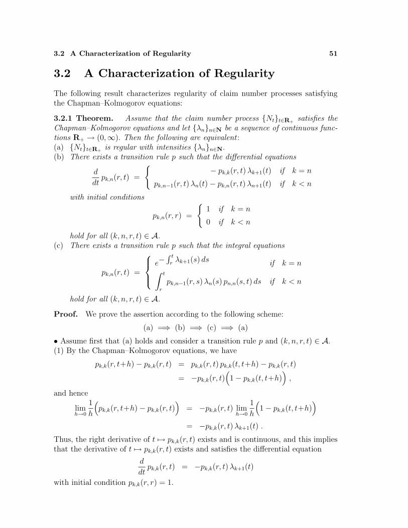
3.2 A Characterization of Regularity 51
3.2 A Characterization of Regularity
The following result characterizes regularity of claim number processes satisfyingthe Chapman–Kolmogorov equations:
3.2.1 Theorem. Assume that the claim number process Ntt∈R+satisfies the
Chapman–Kolmogorov equations and let λnn∈N be a sequence of continuous func-tions R+ → (0,∞). Then the following are equivalent :(a) Ntt∈R+
is regular with intensities λnn∈N.(b) There exists a transition rule p such that the differential equations
d
dtpk,n(r, t) =
− pk,k(r, t) λk+1(t) if k = n
pk,n−1(r, t) λn(t)− pk,n(r, t) λn+1(t) if k < n
with initial conditions
pk,n(r, r) =
1 if k = n
0 if k < n
hold for all (k, n, r, t) ∈ A.(c) There exists a transition rule p such that the integral equations
pk,n(r, t) =
e−∫ t
rλk+1(s) ds if k = n
∫ t
r
pk,n−1(r, s) λn(s) pn,n(s, t) ds if k < n
hold for all (k, n, r, t) ∈ A.
Proof. We prove the assertion according to the following scheme:
(a) =⇒ (b) =⇒ (c) =⇒ (a)
• Assume first that (a) holds and consider a transition rule p and (k, n, r, t) ∈ A.(1) By the Chapman–Kolmogorov equations, we have
pk,k(r, t+h)− pk,k(r, t) = pk,k(r, t) pk,k(t, t+h)− pk,k(r, t)
= −pk,k(r, t)(1− pk,k(t, t+h)
),
and hence
limh→0
1
h
(pk,k(r, t+h)− pk,k(r, t)
)= −pk,k(r, t) lim
h→0
1
h
(1− pk,k(t, t+h)
)
= −pk,k(r, t) λk+1(t) .
Thus, the right derivative of t 7→ pk,k(r, t) exists and is continuous, and this impliesthat the derivative of t 7→ pk,k(r, t) exists and satisfies the differential equation
d
dtpk,k(r, t) = −pk,k(r, t) λk+1(t)
with initial condition pk,k(r, r) = 1.
52 Chapter 3 The Claim Number Process as a Markov Process
In particular, we have
pk,k(r, t) = e−∫ t
rλk+1(s) ds
> 0 .
(2) Assume now that k < n. Then we have
pk,n(r, t+h)− pk,n(r, t) =n∑
m=k
pk,m(r, t) pm,n(t, t+h)− pk,n(r, t)
=n−2∑
m=k
pk,m(r, t) pm,n(t, t+h)
+ pk,n−1(r, t) pn−1,n(t, t+h)
− pk,n(r, t)(1− pn,n(t, t+h)
).
For m ∈ k, . . . , n−2, we have pm,n(t, t+h) ≤ 1 − pm,m(t, t+h) − pm,m+1(t, t+h),hence
limh→0
1
hpm,n(t, t+h) = 0 ,
and this identity together with
limh→0
1
hpn−1,n(t, t+h) = λn(t)
and
limh→0
1
h
(1− pn,n(t, t+h)
)= λn+1(t)
yields
limh→0
1
h
(pk,n(r, t+h)− pk,n(r, t)
)=
n−2∑
m=k
pk,m(r, t) limh→0
1
hpm,n(t, t+h)
+ pk,n−1(r, t) limh→0
1
hpn−1,n(t, t+h)
− pk,n(r, t) limh→0
1
h
(1− pn,n(t, t+h)
)
= pk,n−1(r, t) λn(t)− pk,n(r, t) λn+1(t)) .
Thus, the right derivative of t 7→ pk,n(r, t) exists, and it follows that the functiont 7→ pk,n(r, t) is right continuous on [r,∞). Moreover, for t ∈ (r,∞) the Chapman–Kolmogorov equations yield, for all s ∈ (r, t),
∣∣pk,n(r, s)− pk,n(r, t)∣∣ =
∣∣∣∣∣pk,n(r, s)−n∑
m=k
pk,m(r, s) pm,n(s, t)
∣∣∣∣∣
3.2 A Characterization of Regularity 53
≤n−1∑
m=k
pk,m(r, s) pm,n(s, t) + pk,n(r, s)(1−pn,n(s, t)
)
≤n∑
m=k
(1− pm,m(s, t)
)
=n∑
m=k
(1− pm,m(r, t)
pm,m(r, s)
),
and thus
lims→t
∣∣pk,n(r, s)− pk,n(r, t)∣∣ = 0 ,
which means that the function t 7→ pk,n(r, t) is also left continuous on (r,∞) andhence continuous on [r,∞). But then the right derivative of t 7→ pk,n(r, t) is con-tinuous, and this implies that the derivative of t 7→ pk,n(r, t) exists and satisfies thedifferential equation
d
dtpk,n(r, t) = pk,n−1(r, t) λn(t)− pk,n(r, t) λn+1(t)
with initial condition pk,n(r, r) = 0.(3) Because of (1) and (2), (a) implies (b).• Assume now that (b) holds and consider a transition rule p satisfying the differ-ential equations and (k, n, r, t) ∈ A.(1) We have already noticed in the preceding part of the proof that the differentialequation
d
dtpk,k(r, t) = −pk,k(r, t) λk+1(t)
with initial condition pk,k(r, r) = 1 has the unique solution
pk,k(r, t) = e−∫ t
rλk+1(s) ds .
(2) Assume now that k < n. Then the function t 7→ 0 is the unique solution of thehomogeneous differential equation
d
dtpk,n(r, t) = −pk,n(r, t) λn+1(t)
with initial condition pk,n(r, r) = 0. This implies that the inhomogeneous differentialequation
d
dtpk,n(r, t) = pk,n−1(r, t) λn(t)− pk,n(r, t) λn+1(t)
with initial condition pk,n(r, r) = 0 has at most one solution.
54 Chapter 3 The Claim Number Process as a Markov Process
Assume that the function t 7→ pk,n−1(r, t) is already given (which because of (1) isthe case for n = k + 1) and define
pk,n(r, t) :=
∫ t
r
pk,n−1(r, s) λn(s) pn,n(s, t) ds .
Since
d
dtpk,n(r, t) =
∫ t
r
pk,n−1(r, s) λn(s)
(d
dtpn,n(s, t)
)ds + pk,n−1(r, t) λn(t)
=
∫ t
r
pk,n−1(r, s) λn(s) (−pn,n(s, t) λn+1(t)) ds + pk,n−1(r, t) λn(t)
=
∫ t
r
pk,n−1(r, s) λn(s) pn,n(s, t) ds · (−λn+1(t)) + pk,n−1(r, t) λn(t)
= pk,n(r, s) (−λn+1(t)) + pk,n−1(r, t) λn(t)
= pk,n−1(r, t) λn(t)− pk,n(r, s) λn+1(t)
and pk,n(r, r) = 0, the function t 7→ pk,n(r, t) is the unique solution of the differentialequation
d
dtpk,n(r, t) = pk,n−1(r, t) λn(t)− pk,n(r, t) λn+1(t) ,
with initial condition pk,n(r, r) = 0, and we have
pk,n(r, t) :=
∫ t
r
pk,n−1(r, s) λn(s) pn,n(s, t) ds .
(3) Because of (1) and (2), (b) implies (c).• Assume finally that (c) holds and consider a transition rule p satisfying the integralequations. For n ∈ N and r, t ∈ R+ such that r ≤ t, define
Λn(r, t) :=
∫ t
r
λn(s) ds .
Then we have
pn,n(r, t) = e−∫ t
rλn+1(s) ds
= e−Λn+1(r,t)
> 0
for each admissible pair (n, r) and all t ∈ [r,∞).First, for all t ∈ R+, we have
P [Nt = 0] = P [Nt = 0|N0 = 0]= p0,0(0, t)
> 0 .
3.2 A Characterization of Regularity 55
Consider now t ∈ (0,∞) and assume that p0,n−1(0, t) = P [Nt = n−1] > 0 holdsfor some n ∈ N and all t ∈ R+ (which is the case for n = 1). Then we have
P [Nt = n] = P [Nt = n|N0 = 0]= p0,n(0, t)
=
∫ t
0
p0,n−1(0, s) λn(s) pn,n(s, t) ds
> 0 .
This yields
P [Nt = n] > 0
for each admissible pair (n, t), which proves (i).Second, for each admissible pair (n, t) and for all h ∈ R+, we have
pn,n(t, t+h) = e−Λn+1(t,t+h) ,
showing that the function h 7→ pn,n(t, t+h) is continuous, which proves (ii).Finally, for each admissible pair (n, t), we have
limh→0
1
h
(1− pn,n(t, t+h)
)= lim
h→0
1
h
(1− e−Λn+1(t,t+h)
)
= λn+1(t) ,
and because of
pn,n+1(t, t+h) =
∫ t+h
t
pn,n(t, u) λn+1(u) pn+1,n+1(u, t+h) du
=
∫ t+h
t
pn,n(t, u) λn+1(u) e−Λn+2(u,t+h) du
= e−Λn+2(t,t+h)
∫ t+h
t
pn,n(t, u) λn+1(u) eΛn+2(t,u) du
we also have
limh→0
1
hpn,n+1(t, t+h)
= limh→0
1
h
(e−Λn+2(t,t+h)
∫ t+h
t
pn,n(t, u) λn+1(u) eΛn+2(t,u) du
)
= e−Λn+2(t,t) · pn,n(t, t) λn+1(t) eΛn+2(t,t)
= λn+1(t) .
This proves (iii).Therefore, (c) implies (a). 2
Since regularity is independent of the particular choice of the transition rule, everytransition rule for a regular claim number process satisfying the Chapman–Kolmo-gorov equations fulfills the differential and integral equations of Theorem 3.2.1.
56 Chapter 3 The Claim Number Process as a Markov Process
3.3 A Characterization of the InhomogeneousPoisson Process
In the present section, we study claim number processes which are regular Markovprocesses with intensities which are all identical.
3.3.1 Lemma. Assume that the claim number process Ntt∈R+satisfies the
Chapman–Kolmogorov equations and is regular. Then the following are equivalent :(a) The identity
p0,k(t, t+h) = pn,n+k(t, t+h)
holds for all n, k ∈ N0 and t, h ∈ R+ such that (n, t) is admissible.(b) The intensities of Ntt∈R+
are all identical.
Proof. • It is clear that (a) implies (b).• Assume now that (b) holds.(1) For each admissible pair (n, t) and all h ∈ R+, we have
p0,0(t, t+h) = e−∫ t+h
tλ1(s) ds
= e−∫ t+h
tλn+1(s) ds
= pn,n(t, t+h) .
(2) Assume now that the identity
p0,k(t, t+h) = pn,n+k(t, t+h)
holds for some k ∈ N0 and for each admissible pair (n, t) and all h ∈ R+ (whichbecause of (1) is the case for k = 0). Then we have
p0,k+1(t, t+h) =
∫ t+h
t
p0,k(t, u) λk+1(u) pk+1,k+1(u, t+h) du
=
∫ t+h
t
pn,n+k(t, u) λn+k+1(u) pn+k+1,n+k+1(u, t+h) du
= pn,n+k+1(t, t+h) .
for each admissible pair (n, t) and all h ∈ R+.(3) Because of (1) and (2), (b) implies (a). 2
Let λ : R+ → (0,∞) be a continuous function. The claim number process Ntt∈R+
is an inhomogeneous Poisson process with intensity λ if it has independent incre-ments satisfying
PNt+h−Nt = P(∫ t+h
tλ(s) ds
)
3.3 A Characterization of the Inhomogeneous Poisson Process 57
for all t ∈ R+ and h ∈ (0,∞). Thus, the claim number process is an inhomogeneousPoisson process with constant intensity t 7→ α if and only if it is a Poisson processwith parameter α.
3.3.2 Theorem. Let λ : R+ → (0,∞) be a continuous function. Then thefollowing are equivalent :(a) The claim number process Ntt∈R+
is a regular Markov process with intensitiesλnn∈N satisfying λn(t) = λ(t) for all n∈N and t∈R+.
(b) The claim number process Ntt∈R+has independent increments and is regular
with intensities λnn∈N satisfying λn(t) = λ(t) for all n∈N and t∈R+.(c) The claim number process Ntt∈R+
is an inhomogeneous Poisson process withintensity λ.
Proof. Each of the conditions implies that the claim number process satisfies theChapman–Kolmogorov equations. Therefore, Theorem 3.2.1 applies.For all r, t∈R+ such that r ≤ t, define
Λ(r, t) :=
∫ t
r
λ(s) ds .
We prove the assertion according to the following scheme:
(a) =⇒ (c) =⇒ (b) =⇒ (a)
• Assume first that (a) holds.(1) For each admissible pair (n, r) and all t ∈ [r,∞), we have
pn,n(r, t) = e−∫ t
rλn+1(s) ds
= e−∫ t
rλ(s) ds
= e−Λ(r,t) .
(2) Assume now that the identity
pn,n+k(r, t) = e−Λ(r,t) (Λ(r, t))k
k!
holds for some k ∈ N0 and for each admissible pair (n, r) and all t ∈ [r,∞) (whichbecause of (1) is the case for k = 0). Then we have
pn,n+k+1(r, t) =
∫ t
r
pn,n+k(r, s) λn+k+1(s) pn+k+1,n+k+1(s, t) ds
=
∫ t
r
e−Λ(r,s) (Λ(r, s))k
k!λ(s) e−Λ(s,t) ds
= e−Λ(r,t)
∫ t
r
(Λ(r, s))k
k!λ(s) ds
= e−Λ(r,t) (Λ(r, t))k+1
(k+1)!
for each admissible pair (n, r) and all t ∈ [r,∞).
58 Chapter 3 The Claim Number Process as a Markov Process
(3) Because of (1) and (2), the identity
pn,n+k(r, t) = e−Λ(r,t) (Λ(r, t))k
k!
holds for all n, k ∈ N0 and r, t ∈ R+ such that (n, r) is admissible and r ≤ t.(4) Because of (3), we have
P [Nt = n] = p0,n(0, t)
= e−Λ(0,t) (Λ(0, t))n
n!
for all t ∈ R+ and n ∈ N0 such that (n, t) is admissible, and thus
PNt = P(Λ(0, t)) .
for all t ∈ (0,∞).(5) The identity
PNt−Nr = P(Λ(r, t))
holds for all r, t ∈ R+ such that r < t.In the case r = 0, the assertion follows from (4).In the case r > 0, it follows from (4) that the probability of explosion is equal tozero and that P [Nr = n] > 0 holds for all n ∈ N0. Because of (3), we obtain
P [Nt−Nr = k] =∞∑
n=0
P [Nt−Nr = k∩Nr = n]
=∞∑
n=0
(P [Nt = n + k|Nr = n] · P [Nr = n]
)
=∞∑
n=0
pn,n+k(r, t) p0,n(0, r)
=∞∑
n=0
e−Λ(r,t) (Λ(r, t))k
k!e−Λ(0,r) (Λ(0, r))n
n!
= e−Λ(r,t) (Λ(r, t))k
k!·∞∑
n=0
e−Λ(0,r) (Λ(0, r))n
n!
= e−Λ(r,t) (Λ(r, t))k
k!
for all k ∈ N0, and thus
PNt−Nr = P(Λ(r, t)) .
3.3 A Characterization of the Inhomogeneous Poisson Process 59
(6) The claim number process Ntt∈R+has independent increments :
Consider m ∈ N, t0, t1, . . . , tm ∈ R+ such that 0 = t0 < t1 < . . . < tm, andk1, . . . , km ∈ N0. For j ∈ 0, 1, . . . ,m, define
nj :=
j∑i=1
ki .
If P [⋂m−1
j=1 Ntj−Ntj−1= kj] = P [
⋂m−1j=1 Ntj = nj] > 0, then the Markov property
together with (3) and (5) yields
P
[Ntm = nm
∣∣∣∣∣m−1⋂j=1
Ntj = nj]
= P [Ntm = nm|Ntm−1 = nm−1]
= pnm−1,nm(tm−1, tm)
= e−Λ(tm−1,tm) (Λ(tm−1, tm))nm−nm−1
(nm−nm−1)!
= P [Ntm−Ntm−1 = nm−nm−1]= P [Ntm−Ntm−1 = km]
and hence
P
[m⋂
j=1
Ntj−Ntj−1= kj
]= P
[m⋂
j=1
Ntj = nj]
= P
[Ntm = nm
∣∣∣∣∣m−1⋂j=1
Ntj = nj]· P
[m−1⋂j=1
Ntj = nj]
= P [Ntm−Ntm−1 = km] · P[
m−1⋂j=1
Ntj = nj]
= P [Ntm−Ntm−1 = km] · P[
m−1⋂j=1
Ntj−Ntj−1= kj
].
Obviously, the identity
P
[m⋂
j=1
Ntj−Ntj−1= kj
]= P [Ntm−Ntm−1 = km] · P
[m−1⋂j=1
Ntj−Ntj−1= kj
]
is also valid if P [⋂m−1
j=1 Ntj−Ntj−1= kj] = 0.
It now follows by induction that Ntt∈R+has independent increments.
(7) Because of (5) and (6), Ntt∈R+is an inhomogeneous Poisson process with
intensity λ. Therefore, (a) implies (c).
60 Chapter 3 The Claim Number Process as a Markov Process
• Assume now that (c) holds. Of course, Ntt∈R+has independent increments.
Furthermore, for each admissible pair (n, r) and all k ∈ N0 and t ∈ [r,∞), we have
pn,n+k(r, t) = P [Nt = n+k|Nr = n]= P [Nt−Nr = k|Nr−N0 = n]= P [Nt−Nr = k]
= e−Λ(r,t) (Λ(r, t))k
k!.
For k = 0, this yields
pn,n(r, t) = e−Λ(r,t)
= e−∫ t
rλ(s) ds ,
and for k ∈ N we obtain
pn,n+k(r, t) = e−Λ(r,t) (Λ(r, t))k
k!
= e−Λ(r,t)
∫ t
r
(Λ(r, s))k−1
(k−1)!λ(s) ds
=
∫ t
r
e−Λ(r,s) (Λ(r, s))k−1
(k−1)!λ(s) e−Λ(s,t) ds
=
∫ t
r
pn,n+k−1(r, s) λ(s) pn+k,n+k(s, t) ds .
It now follows from Theorem 3.2.1 that Ntt∈R+is regular with intensities λnn∈N
satisfying λn(t) = λ(t) for all n ∈ N and t ∈ R+. Therefore, (c) implies (b).• Assume finally that (b) holds. Since Ntt∈R+
has independent increments, itfollows from Theorem 3.1.1 that Ntt∈R+
is a Markov process. Therefore, (b) im-plies (a). 2
The following result is a partial generalization of Lemma 2.3.1:
3.3.3 Lemma (Multinomial Criterion). If the claim number process Ntt∈R+
is an inhomogeneous Poisson process with intensity λ, then the identity
P
[m⋂
j=1
Ntj−Ntj−1= kj
∣∣∣∣∣Ntm = n]
=n!∏m
j=1 kj!
m∏j=1
(∫ tjtj−1
λ(s) ds∫ tm
0λ(s) ds
)kj
holds for all m ∈ N and t0, t1, . . . , tm ∈ R+ such that 0 = t0 < t1 < . . . < tm andfor all n ∈ N0 and k1, . . . , km ∈ N0 such that
∑mj=1 kj = n.
3.3 A Characterization of the Inhomogeneous Poisson Process 61
Proof. For all r, t ∈ R+ satisfying r ≤ t, define
Λ(r, t) :=
∫ t
r
λ(s) ds .
Then we have
P
[m⋂
j=1
Ntj−Ntj−1= kj
∣∣∣∣∣Ntm = n]
=
P
[m⋂
j=1
Ntj−Ntj−1= kj
]
P [Ntm = n]
=
m∏j=1
P [Ntj−Ntj−1= kj]
P [Ntm = n]
=
m∏j=1
e−Λ(tj−1,tj)(Λ(tj−1, tj))
kj
kj!
e−Λ(0,tm) (Λ(0, tm))n
n!
=n!∏m
j=1 kj!
m∏j=1
(Λ(tj−1, tj)
Λ(0, tm)
)kj
,
as was to be shown. 2
Problems3.3.A Assume that the claim number process has independent increments and is regular.
Then its intensities are all identical.
3.3.B The following are equivalent:(a) The claim number process is a regular Markov process and its intensities are
all identical.(b) The claim number process has independent increments and is regular.(c) The claim number process is an inhomogeneous Poisson process.
3.3.C Consider a continuous function λ : R+ → (0,∞) satisfying∫∞0 λ(s) ds = ∞. For
all t ∈ R+, define
%(t) :=∫ t
0λ(s) ds
as well asN.
t := N%(t)
andN/
t := N%−1(t) .
(a) If the claim number process Ntt∈R+is a Poisson process with parameter 1,
then N.t t∈R+
is an inhomogeneous Poisson process with intensity λ.(b) If the claim number process Ntt∈R+
is an inhomogeneous Poisson processwith intensity λ, then N/
t t∈R+is a Poisson process with parameter 1.
62 Chapter 3 The Claim Number Process as a Markov Process
3.3.D Consider a continuous function λ : R+ → (0,∞) satisfying∫∞0 λ(s) ds = ∞. For
all t ∈ R+, define
%(t) :=∫ t
0λ(s) ds .
Then the following are equivalent:(a) The claim number process Ntt∈R+
is an inhomogeneous Poisson processwith intensity λ.
(b) The claim number process Ntt∈R+has independent increments and satis-
fies E[Nt] = %(t) for all t ∈ R+.(c) The process Nt − %(t)t∈R+
is a martingale.
3.3.E Prediction: If the claim number process Ntt∈R+is an inhomogeneous Poisson
process with intensity λ, then the inequality
E
[(Nt+h −
(Nt+
∫ t+h
tλ(s) ds
))2]≤ E[(Nt+h − Z)2]
holds for all t, h ∈ R+ and for every random variable Z satisfying E[Z2] < ∞and σ(Z) ⊆ Ft.
3.4 A Characterization of Homogeneity
In the present section, we study claim number processes which are regular Markovprocesses with intensities which are all constant.
3.4.1 Lemma. Assume that the claim number process Ntt∈R+satisfies the
Chapman–Kolmogorov equations and is regular. Then the following are equivalent :
(a) Ntt∈R+is homogeneous.
(b) The intensities of Ntt∈R+are all constant.
Proof. • Assume first that (a) holds and consider n ∈ N0. For all s, t ∈ (0,∞),we have
λn+1(s) = limh→0
1
hpn,n+1(s, s+h)
= limh→0
1
hpn,n+1(t, t+h)
= λn+1(t) .
Thus, λn+1 is constant on (0,∞) and hence, by continuity, on R+. Therefore,(a) implies (b).• Assume now that (b) holds and consider a sequence αnn∈N in (0,∞) such thatλn(t) = αn holds for all n ∈ N and t ∈ R+.
3.4 A Characterization of Homogeneity 63
(1) For all n ∈ N0 and s, t, h ∈ R+ such that (n, s) and (n, t) are admissible, wehave
pn,n(s, s+h) = e−∫ s+h
sλn+1(u) du
= e−∫ s+h
sαn+1 du
= e−αn+1h ,
and hence
pn,n(s, s+h) = pn,n(t, t+h) .
(2) Assume now that the identity
pn,n+k(s, s+h) = pn,n+k(t, t+h)
holds for some k ∈ N0 and for all n ∈ N0 and s, t, h ∈ R+ such that (n, s) and (n, t)are admissible (which because of (1) is the case for k = 0). Then we have
pn,n+k+1(s, s+h) =
∫ s+h
s
pn,n+k(s, u) λn+k+1(u) pn+k+1,n+k+1(u, s+h) du
=
∫ s+h
s
pn,n+k(t, t−s+u) αn+k+1 pn+k+1,n+k+1(t−s+u, t+h) du
=
∫ t+h
t
pn,n+k(t, v) αn+k+1 pn+k+1,n+k+1(v, t+h) dv
=
∫ t+h
t
pn,n+k(t, v) λn+k+1(v) pn+k+1,n+k+1(v, t+h) dv
= pn,n+k+1(t, t+h)
for all n ∈ N0 and s, t, h ∈ R+ such that (n, s) and (n, t) are admissible.(3) Because of (1) and (2), (b) implies (a). 2
The main result of this section is the following characterization of homogeneousregular Markov processes:
3.4.2 Theorem. Let αnn∈N be a sequence of real numbers in (0,∞). Then thefollowing are equivalent :(a) The claim number process Ntt∈R+
is a regular Markov process with intensitiesλnn∈N satisfying λn(t) = αn for all n∈N and t∈R+.
(b) The sequence of claim interarrival times Wnn∈N is independent and satisfiesPWn = Exp(αn) for all n∈N.
Proof. For n ∈ N, let Tn and Wn denote the random vectors Ω → Rn withcoordinates Ti and Wi, respectively, and let Mn denote the (n×n)–matrix withentries
mij :=
1 if i ≥ j0 if i < j .
64 Chapter 3 The Claim Number Process as a Markov Process
Then Mn is invertible and satisfies
detMn = 1 .
Moreover, we have Tn = Mn Wn and hence
Wn = M−1n Tn
as well as T−1n = W−1
n M−1n . Furthermore, let 1n denote the vector in Rn with all
coordinates being equal to one, and let 〈. , .〉 denote the inner product on Rn.• Assume first that (a) holds. Since the claim arrival process is more directly relatedto the claim number process than the claim interarrival process is, we shall firstdetermine the finite dimensional distributions of the claim arrival process and thenapply the identity Wn = M−1
n Tn to obtain the finite dimensional distributions ofthe claim interarrival process.Consider two sequences rjj∈N and tjj∈N0
of real numbers satisfying t0 = 0 andtj−1 ≤ rj < tj for all j ∈ N. We first exploit regularity and then the Markov propertyin order to determine the finite dimensional distributions of the claim arrival process.(1) For each admissible pair (j, r) and all t ∈ [r,∞), we have
pj,j(r, t) = e−αj+1(t−r) .
Indeed, regularity yields
pj,j(r, t) = e−∫ t
rλj+1(s) ds
= e−∫ t
rαj+1 ds
= e−αj+1(t−r) .
(2) For all j ∈ N and r, t ∈ (0,∞) such that r ≤ t, we have
pj−1,j(r, t) =
αj
αj+1−αj
(e−αj(t−r) − e−αj+1(t−r)
)if αj 6= αj+1
αj(t−r) e−αj(t−r) if αj = αj+1 .
Indeed, if αj 6= αj+1, then regularity together with (1) yields
pj−1,j(r, t) =
∫ t
r
pj−1,j−1(r, s) λj(s) pj,j(s, t) ds
=
∫ t
r
e−αj(s−r) αj e−αj+1(t−s) ds
= αj e(αjr−αj+1t)
∫ t
r
e(αj+1−αj)s ds
= αj e(αjr−αj+1t) 1
αj+1−αj
(e(αj+1−αj)t − e(αj+1−αj)r
)
=αj
αj+1−αj
(e−αj(t−r) − e−αj+1(t−r)
);
3.4 A Characterization of Homogeneity 65
similarly, if αj = αj+1, then
pj−1,j(r, t) =
∫ t
r
pj−1,j−1(r, s) λj(s) pj,j(s, t) ds
=
∫ t
r
e−αj(s−r) αj e−αj+1(t−s) ds
=
∫ t
r
e−αj(s−r) αj e−αj(t−s) ds
=
∫ t
r
αj e−αj(t−r) ds
= αj(t−r) e−αj(t−r) .
(3) For all j ∈ N and h ∈ (0,∞), we have
pj−1,j−1(h, h+rj) pj−1,j(rj, tj) pj,j(tj, rj+1)
=
∫ tj
rj
αj e(αj+1−αj)sj dsj · pj,j(h, h+rj+1) .
Indeed, if αj 6= αj+1, then (1) and (2) yield
pj−1,j−1(h, h+rj) pj−1,j(rj, tj) pj,j(tj, rj+1)
= e−αjrj · αj
αj+1−αj
(e−αj(tj−rj) − e−αj+1(tj−rj)
)· e−αj+1(rj+1−tj)
=αj
αj+1−αj
(e(αj+1−αj)tj − e(αj+1−αj)rj
)· e−αj+1rj+1
=
∫ tj
rj
αj e(αj+1−αj)sj dsj · pj,j(h, h+rj+1) ;
similarly, if αj = αj+1, then
pj−1,j−1(h, h+rj) pj−1,j(rj, tj) pj,j(tj, rj+1)
= e−αjrj · αj(tj−rj) e−αj(tj−rj) · e−αj+1(rj+1−tj)
= e−αjrj · αj(tj−rj) e−αj(tj−rj) · e−αj(rj+1−tj)
= αj(tj−rj) · e−αjrj+1
=
∫ tj
rj
αj dsj · pj,j(h, h+rj+1)
=
∫ tj
rj
αj e(αj+1−αj)sj dsj · pj,j(h, h+rj+1) .
66 Chapter 3 The Claim Number Process as a Markov Process
(4) For all n ∈ N, we have
P
[Nrn = n−1 ∩
n−1⋂j=1
Ntj = j∩Nrj= j−1
]> 0
and
P
[n⋂
j=1
Ntj = j∩Nrj= j−1
]> 0 .
This follows by induction, using (1) and (2) and the Markov property:For n = 1, we have
P [Nr1 = 0] = P [Nr1 = 0|N0 = 0]= p0,0(0, r1)
> 0
and
P [Nt1 = 1∩Nr1 = 0] = P [Nt1 = 1|Nr1 = 0] · P [Nr1 = 0]= p0,0(0, r1) p0,1(r1, t1)
> 0 .
Assume now that the assertion holds for some n ∈ N. Then we have
P
[Nrn+1 = n ∩
n⋂j=1
Ntj = j∩Nrj= j−1
]
= P
[Nrn+1 = n
∣∣∣∣∣n⋂
j=1
Ntj = j∩Nrj= j−1
]
·P[
n⋂j=1
Ntj = j∩Nrj= j−1
]
= P [Nrn+1 = n|Ntn = n]
·P[
n⋂j=1
Ntj = j∩Nrj= j−1
]
= pn,n(tn, rn+1) · P[
n⋂j=1
Ntj = j∩Nrj= j−1
]
> 0
3.4 A Characterization of Homogeneity 67
and
P
[n+1⋂j=1
Ntj = j∩Nrj= j−1
]
= P
[Ntn+1 = n+1
∣∣∣∣∣Nrn+1 = n ∩n⋂
j=1
Ntj = j∩Nrj= j−1
]
·P[Nrn+1 = n ∩
n⋂j=1
Ntj = j∩Nrj= j−1
]
= P [Ntn+1 = n+1|Nrn+1 = n]
·P[Nrn+1 = n ∩
n⋂j=1
Ntj = j∩Nrj= j−1
]
= pn,n+1(rn+1, tn+1) · P[Nrn+1 = n ∩
n⋂j=1
Ntj = j∩Nrj= j−1
]
> 0 .
(5) For all n ∈ N, we have
P
[n⋂
j=1
rj < Tj ≤ tj]
=n−1∏j=1
∫ tj
rj
αje(αj+1−αj)sj dsj ·
∫ tn
rn
αneαnsn dsn .
Indeed, using (4), the Markov property, (3), and (1), we obtain, for all h ∈ (0,∞),
P
[n⋂
j=1
rj < Tj ≤ tj]
= P
[n⋂
j=1
Nrj< j ≤ Ntj
]
= P
[Ntn ≥ n∩Nrn = n−1 ∩
n−1⋂j=1
Ntj = j∩Nrj= j−1
]
= P [Ntn ≥ n|Nrn = n−1]
·n−1∏j=1
(P [Nrj+1
= j|Ntj = j] · P [Ntj = j|Nrj= j−1]
)
· P [Nr1 = 0|N0 = 0]
= p0,0(0, r1) ·n−1∏j=1
pj−1,j(rj, tj) pj,j(tj, rj+1) ·(1− pn−1,n−1(rn, tn)
)
68 Chapter 3 The Claim Number Process as a Markov Process
= p0,0(h, h+r1) ·n−1∏j=1
pj−1,j(rj, tj) pj,j(tj, rj+1) ·(1− pn−1,n−1(rn, tn)
)
=n−1∏j=1
∫ tj
rj
αj e(αj+1−αj)sj dsj · pn−1,n−1(h, h+rn) ·(1− pn−1,n−1(rn, tn)
)
=n−1∏j=1
∫ tj
rj
αj e(αj+1−αj)sj dsj · e−αnrn ·(1− e−αn(tn−rn)
)
=n−1∏j=1
∫ tj
rj
αj e(αj+1−αj)sj dsj ·(e−αnrn − e−αntn
)
=n−1∏j=1
∫ tj
rj
αj e(αj+1−αj)sj dsj ·∫ tn
rn
αn e−αnsn dsn .
(6) Consider n ∈ N and define fn : Rn → R+ by letting
fn(w) :=n∏
j=1
αj e−αjwjχ(0,∞)(wj) .
Define s0 := 0 and A :=×nj=1(rj, tj]. Because of (5), we obtain
P [Tn ∈ A] = P
[n⋂
j=1
rj < Tj ≤ tj]
=n−1∏j=1
∫ tj
rj
αj e(αj+1−αj)sj dsj ·∫ tn
rn
αn e−αnsn dsn
=n−1∏j=1
∫
(rj ,tj ]
αj e(αj+1−αj)sj dλ(sj) ·∫
(rn,tn]
αn e−αnsn dλ(sn)
=
∫
A
(n−1∏j=1
αj e(αj+1−αj)sj
)αn e−αnsn dλ
n
(s)
=
∫
A
(n∏
j=1
αj e−αj(sj−sj−1)χ(0,∞)(sj−sj−1)
)dλ
n
(s)
=
∫
A
fn(M−1n (s)) dλ
n
(s) .
(7) Since the sequence Tnn∈N0is strictly increasing with T0 = 0, it follows from (6)
that the identity
P [Tn ∈ A] =
∫
A
fn(M−1n (s)) dλ
n
(s)
holds for all A ∈ B(Rn).
3.4 A Characterization of Homogeneity 69
(8) Consider B1, . . . , Bn ∈ B(R) and let B :=×nj=1Bj. Since Wn = M−1
n Tn, theidentity established in (7) yields
PWn[B] = P [Wn ∈ B]
= P [M−1n Tn ∈ B]
= P [Tn ∈ Mn(B)]
=
∫
Mn(B)
fn(M−1n (s)) dλ
n
(s)
=
∫
B
fn(w) dλn
M−1n
(w)
=
∫
B
fn(w)1
| detM−1n | dλ
n
(w)
=
∫
B
fn(w) dλn
(w)
=
∫
B
(n∏
j=1
αj e−αjwjχ(0,∞)(wj)
)dλ
n
(w)
=n∏
j=1
∫
Bj
αj e−αjwjχ(0,∞)(wj) dλ(wj) .
(9) Because of (8), the sequence Wnn∈N is independent and satisfies
PWn = Exp(αn)
for all n ∈ N. Therefore, (a) implies (b).• Assume now that (b) holds.(1) To establish the Markov property, consider m ∈ N, t1, . . . , tm, tm+1 ∈ (0,∞),and k1, . . . , km ∈ N0 such that t1 < . . . < tm < tm+1 and P [
⋂mj=1Ntj = kj] > 0.
In the case where km = 0, it is clear that the identity
P
[Ntm+1 = km+1
∣∣∣∣∣m⋂
j=1
Ntj = kj]
= P [Ntm+1 = l|Ntm = km]
holds for all km+1 ∈ N0 such that km ≤ km+1.In the case where km ∈ N, define k0 := 0 and n := km, and let l ∈ 0, 1, . . . ,m−1be the unique integer satisfying kl < kl+1 = km = n. Then there exists a rectangleB ⊆×n
j=1(0, tl+1] such that
(l⋂
j=1
Tkj≤ tj < Tkj+1
)∩Tn ≤ tl+1 = T−1
n (B) .
70 Chapter 3 The Claim Number Process as a Markov Process
Letting A := M−1n (B), we obtain
(l⋂
j=1
Tkj≤ tj < Tkj+1
)∩Tn ≤ tl+1 = T−1
n (B)
= W−1n (M−1
n (B))
= W−1n (A) .
Using independence of Wn and Wn+1, the transformation formula for integrals, andFubini’s theorem, we obtain
P
[m⋂
j=1
Ntj = kj]
= P
[(l⋂
j=1
Ntj = kj)∩Ntl+1
= n∩Ntm = n]
= P
[(l⋂
j=1
Tkj≤ tj < Tkj+1
)∩Tn ≤ tl+1∩tm < Tn+1
]
= P [W−1n (A) ∩tm−Tn < Wn+1]
= P [W−1n (A) ∩tm−〈1n,Wn〉 < Wn+1]
=
∫
A
(∫
(tm−〈1n,s〉,∞)
dPWn+1(w)
)dPWn
(s)
=
∫
A
(∫
(tm−〈1n,s〉,∞)
αn+1 e−αn+1w dλ(w)
)dPWn
(s)
=
∫
A
eαn+1〈1n,s〉(∫
(tm,∞)
αn+1 e−αn+1v dλ(v)
)dPWn
(s)
=
∫
A
eαn+1〈1n,s〉 dPWn(s) ·
∫
(tm,∞)
dPWn+1(v) .
Also, using the same arguments as before, we obtain
P [Ntm = km] = P [Ntm = n]= P [Tn ≤ tm < Tn+1]= P [Tn ≤ tm∩tm−Tn < Wn+1]
=
∫
(−∞,tm]
(∫
(tm−s,∞)
dPWn+1(w)
)dPTn(s)
=
∫
(−∞,tm]
(∫
(tm−s,∞)
αn+1 e−αn+1w dλ(w)
)dPTn(s)
=
∫
(−∞,tm]
eαn+1s
(∫
(tm,∞)
αn+1 e−αn+1v dλ(v)
)dPTn(s)
=
∫
(−∞,tm]
eαn+1s dPTn(s) ·∫
(tm,∞)
dPWn+1(v) .

3.4 A Characterization of Homogeneity 71
Consider now k ∈ N0 such that km < k, and define U := Tk−Tn+1 = Tk−Tn−Wn+1.Then we have
P
[Ntm+1 ≥ k ∩
m⋂j=1
Ntj = kj]
= P
[(l⋂
j=1
Ntj = kj)∩Ntl+1
= n∩Ntm = n∩Ntm+1 ≥ k]
= P
[(l⋂
j=1
Tkj≤ tj < Tkj+1
)∩Tn ≤ tl+1∩tm < Tn+1∩Tk ≤ tm+1
]
= P [W−1n (A) ∩tm−Tn < Wn+1∩U ≤ tm+1−Tn−Wn+1]
= P [W−1n (A) ∩tm−〈1n,Wn〉 < Wn+1∩U ≤ tm+1−〈1n,Wn〉−Wn+1]
=
∫
A
(∫
(tm−〈1n,s〉,∞)
(∫
(−∞,tm+1−〈1n,s〉−w]
dPU(u)
)dPWn+1(w)
)dPWn
(s)
=
∫
A
(∫
(tm−〈1n,s〉,∞)
P [U ≤ tm+1−〈1n, s〉−w] dPWn+1(w)
)dPWn
(s)
=
∫
A
(∫
(tm−〈1n,s〉,∞)
P [U ≤ tm+1−〈1n, s〉−w] αn+1 e−αn+1w dλ(w)
)dPWn
(s)
=
∫
A
eαn+1〈1n,s〉(∫
(tm,∞)
P [U ≤ tm+1−v] αn+1 e−αn+1v dλ(v)
)dPWn
(s)
=
∫
A
eαn+1〈1n,s〉 dPWn(s) ·
∫
(tm,∞)
P [U ≤ tm+1−v] dPWn+1(v)
as well as
P [Ntm+1 ≥ k∩Ntm = km]= P [Ntm+1 ≥ k∩Ntm = n]= P [Tn ≤ tm < Tn+1∩Tk ≤ tm+1]= P [Tn ≤ tm∩tm−Tn < Wn+1∩U ≤ tm+1−Tn−Wn+1]=
∫
(−∞,tm]
(∫
(tm−s,∞)
(∫
(−∞,tm+1−s−w]
dPU(u)
)dPWn+1(w)
)dPTn(s)
=
∫
(−∞,tm]
(∫
(tm−s,∞)
P [U ≤ tm+1−s−w] dPWn+1(w)
)dPTn(s)
=
∫
(−∞,tm]
(∫
(tm−s,∞)
P [U ≤ tm+1−s−w] αn+1 e−αn+1w dλ(w)
)dPTn(s)
=
∫
(−∞,tm]
eαn+1s
(∫
(tm,∞)
P [U ≤ tm+1−v] αn+1 e−αn+1v dλ(v)
)dPTn(s)
=
∫
(−∞,tm]
eαn+1s dPTn(s) ·∫
(tm,∞)
P [U ≤ tm+1−v] dPWn+1 .
72 Chapter 3 The Claim Number Process as a Markov Process
This yields
P
[Ntm+1 ≥ k
∣∣∣∣∣m⋂
j=1
Ntj = kj]
=
P
[Ntm+1 ≥ k ∩
m⋂j=1
Ntj = kj]
P
[m⋂
j=1
Ntj = kj]
=
∫
A
eαn+1〈1n,s〉 dPWn(s) ·
∫
(tm,∞)
P [U ≤ tm+1−v] dPWn+1(v)
∫
A
eαn+1〈1n,s〉 dPWn(s) ·
∫
(tm,∞)
dPWn+1(v)
=
∫
(tm,∞)
P [U ≤ tm+1−v] dPWn+1(v)
∫
(tm,∞)
dPWn+1(v)
=
∫
(−∞,tm]
eαn+1s dPTn(s) ·∫
(tm,∞)
P [U ≤ tm+1−v] dPWn+1(v)
∫
(−∞,tm]
eαn+1s dPTn(s) ·∫
(tm,∞)
dPWn+1(v)
=P [Ntm+1 ≥ k ∩ Ntm = km]
P [Ntm = km]= P [Ntm+1 ≥ k|Ntm = km] .
Therefore, we have
P
[Ntm+1 ≥ k
∣∣∣∣∣m⋂
j=1
Ntj = kj]
= P [Ntm+1 ≥ k|Ntm = km]
for all k ∈ N0 such that km < k.Of course, the previous identity is also valid if km = k, and it thus holds for allk ∈ N0 such that km ≤ k. But this implies that the identity
P
[Ntm+1 = km+1
∣∣∣∣∣m⋂
j=1
Ntj = kj]
= P [Ntm+1 = km+1|Ntm = km]
holds for all km+1 ∈ N0 such that km ≤ km+1, which means that Ntt∈R+is a
Markov process.
3.4 A Characterization of Homogeneity 73
(2) To prove the assertion on regularity, consider an admissible pair (n, t). As before,we obtain
P [Nt+h = n∩Nt = n] = P [Tn ≤ t∩t+h < Tn+1]= P [Tn ≤ t∩t+h−Tn < Wn+1]
=
∫
(−∞,t]
(∫
(t+h−s,∞]
dPWn+1(w)
)dPTn(s)
=
∫
(−∞,t]
(∫
(t+h−s,∞]
αn+1 e−αn+1w dλ(w)
)dPTn(s)
=
∫
(−∞,t]
e−αn+1(t+h−s) dPTn(s)
= e−αn+1(t+h)
∫
(−∞,t]
eαn+1s dPTn(s)
for all h ∈ R+, hence
P [Nt = n] = e−αn+1t
∫
(−∞,t]
eαn+1s dPTn(s)
> 0 ,
and thus
pn,n(t, t+h) = P [Nt+h = n|Nt = n]
=P [Nt+h = n∩Nt = n]
P [Nt = n]
=
e−αn+1(t+h)
∫
(−∞,t]
eαn+1s dPTn(s)
e−αn+1t
∫
(−∞,t]
eαn+1s dPTn(s)
= e−αn+1h
for all h ∈ R+.By what we have shown so far, we have
P [Nt = n] > 0 ,
which proves (i).It is also clear that the function h 7→ pn,n(t, t+h) is continuous, which proves (ii).Furthermore, we have
limh→0
1
h
(1− pn,n(t, t+h)
)= lim
h→0
1
h
(1− e−αn+1h
)
= αn+1 .
74 Chapter 3 The Claim Number Process as a Markov Process
Also, we have
P [Nt+h = n+1∩Nt = n]= P [Tn ≤ t < Tn+1 ≤ t+h < Tn+2]= P [Tn ≤ t∩t−Tn < Wn+1 ≤ t+h−Tn∩t+h−Tn−Wn+1 < Wn+2]
=
∫
(−∞,t]
(∫
(t−s,t+h−s]
(∫
(t+h−s−w,∞]
dPWn+2(u)
)dPWn+1(w)
)dPTn(s)
=
∫
(−∞,t]
(∫
(t−s,t+h−s]
(∫
(t+h−s−w,∞]
αn+2 e−αn+2u dλ(u)
)dPWn+1(w)
)dPTn(s)
=
∫
(−∞,t]
(∫
(t−s,t+h−s]
e−αn+2(t+h−s−w) dPWn+1(w)
)dPTn(s)
=
∫
(−∞,t]
(∫
(t−s,t+h−s]
e−αn+2(t+h−s−w) αn+1 e−αn+1w dλ(w)
)dPTn(s)
=
∫
(−∞,t]
(∫
(t,t+h]
e−αn+2(t+h−v) αn+1 e−αn+1(v−s) dλ(v)
)dPTn(s)
= αn+1 e−αn+2(t+h)
∫
(−∞,t]
eαn+1s dPTn(s)
∫
(t,t+h]
e(αn+2−αn+1)v dλ(v) ,
and thus
P [Nt+h = n+1|Nt = n]
=P [Nt+h = n+1∩Nt = n]
P [Nt = n]
=
αn+1 e−αn+2(t+h)
∫
(−∞,t]
eαn+1s dPTn(s)
∫
(t,t+h]
e(αn+2−αn+1)v dλ(v)
e−αn+1t
∫
(−∞,t]
eαn+1s dPTn(s)
= αn+1 eαn+1t e−αn+2(t+h)
∫
(t,t+h]
e(αn+2−αn+1)v dλ(v) .
In the case αn+1 6= αn+2, we obtain
pn,n+1(t, t+h) = P [Nt+h = n+1|Nt = n]
= αn+1 eαn+1t e−αn+2(t+h)
∫
(t,t+h]
e(αn+2−αn+1)v dλ(v)
= αn+1 eαn+1t e−αn+2(t+h) eαn+2−αn+1)(t+h) − e(αn+2−αn+1)t
αn+2 − αn+1
=αn+1
αn+2−αn+1
(e−αn+1h − e−αn+2h
),
3.4 A Characterization of Homogeneity 75
and thus
limh→0
1
hpn,n+1(t, t+h) = lim
h→0
1
h
αn+1
αn+2−αn+1
(e−αn+1h − e−αn+2h
)
= αn+1 ;
in the case αn+1 = αn+2, we obtain
pn,n+1(t, t+h) = P [Nt+h = n+1|Nt = n]
= αn+1 eαn+1t e−αn+2(t+h)
∫
(t,t+h]
e(αn+2−αn+1)v dλ(v)
= αn+1 eαn+1t e−αn+1(t+h)
∫
(t,t+h]
dλ(v)
= αn+1h e−αn+1h ,
and thus
limh→0
1
hpn,n+1(t, t+h) = lim
h→0
1
hαn+1h e−αn+1h
= αn+1 .
Thus, in either case we have
limh→0
1
h
(1− pn,n(t, t+h)
)= αn+1
= limh→0
1
hpn,n+1(t, t+h) .
This proves (iii).We have thus shown that Ntt∈R+
is regular with intensities λnn∈N satisfyingλn(t) = αn for all n ∈ N and t ∈ R+. Therefore, (b) implies (a). 2
In the situation of Theorem 3.4.2, explosion is either certain or impossible:
3.4.3 Corollary (Zero–One Law on Explosion). Let αnn∈N be a sequenceof real numbers in (0,∞) and assume that the claim number process Ntt∈R+
is aregular Markov process with intensities λnn∈N satisfying λn(t) = αn for all n∈Nand t∈R+.(a) If the series
∑∞n=1 1/αn diverges, then the probability of explosion is equal to
zero.(b) If the series
∑∞n=1 1/αn converges, then the probability of explosion is equal to
one.
This follows from Theorems 3.4.2 and 1.2.1.
76 Chapter 3 The Claim Number Process as a Markov Process
Problems3.4.A The following are equivalent:
(a) The claim number process is a regular Markov process and its intensities areall constant.
(b) The claim interarrival times are independent and exponentially distributed.
3.4.B Let % : R+ → R+ be a continuous function which is strictly increasing andsatisfies %(0) = 0 and limt→∞ %(t) = ∞. For all t ∈ R+, define
N%t := N%−1(t) .
Then N%t t∈R+
is a claim number process. Moreover, if Ntt∈R+has indepen-
dent increments or is a Markov process or satisfies the Chapman-Kolmogorovequations or is regular, then the same is true for N%
t t∈R+.
3.4.C Operational Time: A continuous function % : R+ → R+ which is strictlyincreasing and satisfies %(0) = 0 and limt→∞ %(t) = ∞ is an operational time forthe claim number process Ntt∈R+
if the claim number process N%t t∈R+
ishomogeneous.Assume that the claim number process Ntt∈R+
satisfies the Chapman–Kolmo-gorov equations and is regular with intensities λnn∈N, and let αnn∈N be asequence of real numbers in (0,∞). Then the following are equivalent:(a) There exists an operational time % for the claim number process Ntt∈R+
such that λ%n(t) = αn holds for all n ∈ N and t ∈ R+.
(b) There exists a continuous function λ : R+ → (0,∞) satisfying∫∞0 λ(s) ds =
∞ and such that λn(t) = αnλ(t) holds for all n ∈ N and t ∈ R+.Hint : Use Theorem 3.2.1 and choose λ and %, respectively, such that the identity%(t) =
∫ t0 λ(s) ds holds for all t ∈ R+.
3.4.D Operational Time: If Ntt∈R+is an inhomogeneous Poisson process with
intensity λ satisfying∫∞0 λ(s) ds = ∞, then there exists an operational time %
such that N%t t∈R+
is a homogeneous Poisson process with parameter 1.
3.4.E Operational Time: Study the explosion problem for claim number processeswhich are regular Markov processes and possess an operational time.
3.5 A Characterization of the Poisson Process
By Theorem 3.1.8, the Poisson process is a regular Markov process whose intensitiesare all identical and constant. By Theorems 3.3.2, 3.4.2, and 2.3.4, regular Markovprocesses whose intensities are either all identical or all constant share some of thecharacteristic properties of the Poisson process:
– For a regular Markov process whose intensities are all identical, the incrementsof the claim number process are independent and Poisson distributed.
– For a regular Markov process whose intensities are all constant, the claim inter-arrival times are independent and exponentially distributed.
3.6 A Claim Number Process with Contagion 77
In the first case, the intensities are related to the parameters of the distributions ofthe increments of the claim number process; in the second case, they are related tothe parameters of the distributions of the claim interarrival times. It is thereforenot surprising that the Poisson process is the only regular Markov process whoseintensities are all identical and constant:
3.5.1 Theorem. Let α ∈ (0,∞). Then the following are equivalent :(a) The claim number process Ntt∈R+
is a regular Markov process with intensitiesλnn∈N satisfying λn(t) = α for all n∈N and t∈R+.
(b) The claim number process Ntt∈R+has independent increments and is regular
with intensities λnn∈N satisfying λn(t) = α for all n ∈ N and t ∈ R+.(c) The claim number process Ntt∈R+
is a Poisson process with parameter α.(d) The sequence of claim interarrival times Wnn∈N is independent and satisfies
PWn = Exp(α) for all n∈N.
Proof. The equivalence of (a), (b), and (c) follows from Theorem 3.3.2, and theequivalence of (a) and (d) follows from Theorem 3.4.2. 2
The equivalence of (c) and (d) in Theorem 3.5.1 is the same as the equivalence of(a) and (b) in Theorem 2.3.4, which was established by entirely different arguments;in particular, Theorem 2.3.4 was not used in the proof of Theorem 3.5.1.
Problems3.5.A Assume that the claim number process has stationary independent increments
and is regular. Then its intensities are all identical and constant.
3.5.B The following are equivalent:(a) The claim number process is a regular Markov process and its intensities are
all identical and constant.(b) The claim number process has stationary independent increments and is
regular.(c) The claim number process is a Poisson process.(d) The claim interarrival times are independent and identically exponentially
distributed.
3.6 A Claim Number Process with Contagion
In the present section we study a regular claim number process which is homogeneousand satisfies the Chapman–Kolmogorov equations but need not be a Markov processand fails to be a Poisson process. More precisely, the increments of this claim numberprocess fail to be independent, fail to be stationary, and fail to be Poisson distributed.In other words, this claim number process lacks each of the defining properties ofthe Poisson process.
78 Chapter 3 The Claim Number Process as a Markov Process
3.6.1 Theorem (Positive Contagion). Let α, β ∈ (0,∞). Then the followingare equivalent :(a) The claim number process Ntt∈R+
satisfies the Chapman–Kolmogorov equa-tions and is regular with intensities λnn∈N satisfying
λn(t) = (α + n− 1) β
for all n∈N and t∈R+.(b) The identity
pn,n+k(t, t+h) =
(α + n + k − 1
k
)(e−βh
)α+n(1− e−βh
)k
holds for each admissible pair (n, t) and all k∈N0 and h∈R+.In this case, the claim number process is homogeneous and satisfies
PNt = NB(α, e−βt
)
for all t ∈ (0,∞), and the increments are neither independent nor stationary andsatisfy
PNt+h−Nt = NB
(α,
1
1 + eβ(t+h) − eβt
)
for all t∈R+ and h∈(0,∞).
Proof. • Assume first that (a) holds.(1) For each admissible pair (n, t) and all h ∈ R+, we have
pn,n(t, t+h) = e−∫ t+h
tλn+1(u) du
= e−∫ t+h
t(α+n)β du
=(e−βh
)α+n.
(2) Assume now that the identity
pn,n+k(t, t+h) =
(α + n + k − 1
k
)(e−βh
)α+n(1− e−βh
)k
holds for some k ∈ N0 and for each admissible pair (n, t) and all h ∈ R+ (whichbecause of (1) is the case for k = 0). Then we have
pn,n+k+1(t, t+h) =
∫ t+h
t
pn,n+k(t, u) λn+k+1(u) pn+k+1,n+k+1(u, t+h) du
=
∫ t+h
t
((α + n + k − 1
k
)(e−β(u−t)
)α+n(1− e−β(u−t)
)k
·(α + n + k)β
(e−β(t+h−u)
)α+n+k+1
)du
3.6 A Claim Number Process with Contagion 79
=
(α + n + (k + 1)− 1
k + 1
)(e−βh
)α+n
·∫ t+h
t
(k + 1)(1− e−β(u−t)
)k (e−β(t+h−u)
)k+1β du
=
(α + n + (k + 1)− 1
k + 1
)(e−βh
)α+n
·∫ t+h
t
(k + 1)(e−β(t+h−u) − e−βh
)ke−β(t+h−u) β du
=
(α + n + (k + 1)− 1
k + 1
)(e−βh
)α+n(1− e−βh
)k+1
for each admissible pair (n, t) and all h ∈ R+.(3) Because of (1) and (2), (a) implies (b).• Assume now that (b) holds.(1) To verify the Chapman–Kolmogorov equations, consider (k, n, r, t) ∈ A ands ∈ [r, t] such that P [Nr = k] > 0.In the case r = t, there is nothing to prove.In the case r < t, we have
n∑
m=k
pk,m(r, s) pm,n(s, t)
=n∑
m=k
((α + m− 1
m− k
)(e−β(s−r)
)α+k(1− e−β(s−r)
)m−k
·(
α + n− 1
n−m
)(e−β(t−s)
)α+m(1− e−β(t−s)
)n−m
)
=n∑
m=k
((α + n− 1
n− k
)(e−β(t−r)
)α+k (1− e−β(t−r)
)n−k
·(
n− k
m− k
)(e−β(t−s) − e−β(t−r)
1− e−β(t−r)
)m−k (1− e−β(t−s)
1− e−β(t−r)
)(n−k)−(m−k))
=
(α + n− 1
n− k
)(e−β(t−r)
)α+k (1− e−β(t−r)
)n−k
·n∑
m=k
(n− k
m− k
)(e−β(t−s) − e−β(t−r)
1− e−β(t−r)
)m−k (1− e−β(t−s)
1− e−β(t−r)
)(n−k)−(m−k)
=
(α + k + (n−k)− 1
n− k
)(e−β(t−r)
)α+k (1− e−β(t−r)
)n−k
= pk,n(r, t) .
Therefore, Ntt∈R+satisfies the Chapman–Kolmogorov equations.
80 Chapter 3 The Claim Number Process as a Markov Process
(2) To prove the assertion on regularity, consider an admissible pair (n, t).First, since
P [Nt = n] = p0,n(0, t)
=
(α + n− 1
n
)(e−βt
)α(1− e−βt
)n,
we have P [Nt = n] > 0, which proves (i).Second, since
pn,n(t, t+h) =(e−βh
)α+n
= e−(α+n)βh ,
the function h 7→ pn,n(t, t+h) is continuous, which proves (ii).Finally, we have
limh→0
1
h
(1− pn,n(t, t+h)
)= lim
h→0
1
h
(1− e−(α+n)βh
)
=(α + n
)β ,
as well as
limh→0
1
hpn,n+1(t, t+h) = lim
h→0
1
h
(α + n
)(e−βh
)α+n(1− e−βh
)
=(α + n
)β .
This proves (iii).We have thus shown that Ntt∈R+
is regular with intensities λnn∈N satisfyingλn(t) = (α + n− 1) β for all n ∈ N and t ∈ R+.(3) Because of (1) and (2), (b) implies (a).• Let us now prove the final assertions.(1) Consider t ∈ R+. For all n ∈ N0, we have
P [Nt = n] = p0,n(0, t)
=
(α + n− 1
n
)(e−βt
)α(1− e−βt
)n.
This yields
PNt = NB(α, e−βt
).
(2) Consider now t, h ∈ R+. Because of (1), we have, for all k ∈ N0,
P [Nt+h −Nt = k]
=∞∑
n=0
P [Nt+h −Nt = k∩Nt = n]
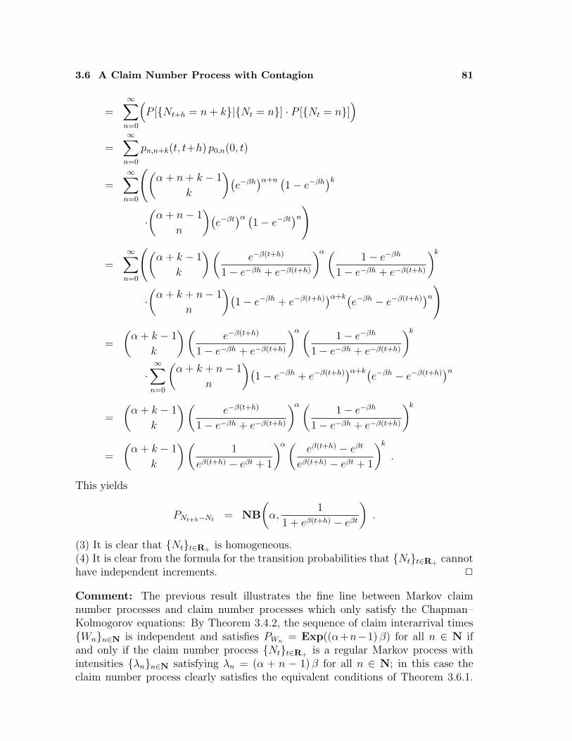
3.6 A Claim Number Process with Contagion 81
=∞∑
n=0
(P [Nt+h = n + k|Nt = n] · P [Nt = n]
)
=∞∑
n=0
pn,n+k(t, t+h) p0,n(0, t)
=∞∑
n=0
((α + n + k − 1
k
)(e−βh
)α+n (1− e−βh
)k
·(
α + n− 1
n
)(e−βt
)α (1− e−βt
)n
)
=∞∑
n=0
((α + k − 1
k
)(e−β(t+h)
1− e−βh + e−β(t+h)
)α (1− e−βh
1− e−βh + e−β(t+h)
)k
·(
α + k + n− 1
n
)(1− e−βh + e−β(t+h)
)α+k(e−βh − e−β(t+h)
)n
)
=
(α + k − 1
k
)(e−β(t+h)
1− e−βh + e−β(t+h)
)α (1− e−βh
1− e−βh + e−β(t+h)
)k
·∞∑
n=0
(α + k + n− 1
n
)(1− e−βh + e−β(t+h)
)α+k(e−βh − e−β(t+h)
)n
=
(α + k − 1
k
)(e−β(t+h)
1− e−βh + e−β(t+h)
)α (1− e−βh
1− e−βh + e−β(t+h)
)k
=
(α + k − 1
k
)(1
eβ(t+h) − eβt + 1
)α (eβ(t+h) − eβt
eβ(t+h) − eβt + 1
)k
.
This yields
PNt+h−Nt = NB
(α,
1
1 + eβ(t+h) − eβt
).
(3) It is clear that Ntt∈R+is homogeneous.
(4) It is clear from the formula for the transition probabilities that Ntt∈R+cannot
have independent increments. 2
Comment: The previous result illustrates the fine line between Markov claimnumber processes and claim number processes which only satisfy the Chapman–Kolmogorov equations: By Theorem 3.4.2, the sequence of claim interarrival timesWnn∈N is independent and satisfies PWn = Exp((α+n−1) β) for all n ∈ N ifand only if the claim number process Ntt∈R+
is a regular Markov process withintensities λnn∈N satisfying λn = (α + n − 1) β for all n ∈ N; in this case theclaim number process clearly satisfies the equivalent conditions of Theorem 3.6.1.
82 Chapter 3 The Claim Number Process as a Markov Process
On the other hand, the equivalent conditions of Theorem 3.6.1 involve only thetwo–dimensional distributions of the claim number process, which clearly cannottell anything about whether the claim number process is a Markov process or not.
The following result justifies the term positive contagion:
3.6.2 Corollary (Positive Contagion). Let α, β ∈ (0,∞) and assume that theclaim number process Ntt∈R+
satisfies the Chapman–Kolmogorov equations and isregular with intensities λnn∈N satisfying
λn(t) = (α + n− 1) β
for all n∈N and t∈R+. Then, for all t, h ∈ (0,∞), the function
n 7→ P [Nt+h ≥ n+1|Nt = n]
is strictly increasing and independent of t.
Thus, in the situation of Corollary 3.6.2, the conditional probability of at least oneclaim occurring in the interval (t, t+h] increases with the number of claims alreadyoccurred up to time t.
The claim number process considered in this section illustrates the importance ofthe negativebinomial distribution.
Another regular claim number process which is not homogeneous but has station-ary increments and which is also related to the negativebinomial distribution andpositive contagion will be studied in Chapter 4 below.
Problems3.6.A Negative Contagion: For α ∈ N, modify the definitions given in Section 3.1
by replacing the set N0∪∞ by 0, 1, . . . , α.Let α ∈ N and β ∈ (0,∞). Then the following are equivalent:(a) The claim number process Ntt∈R+
satisfies the Chapman–Kolmogorovequations and is regular with intensities λnn∈N satisfying
λn(t) = (α + 1− n) β
for all n ∈ 1, . . . , α and t ∈ R+.(b) The identity
pn,n+k(t, t+h) =(
α− n
k
)(1− e−βh
)k(e−βh
)α−n−k
holds for each admissible pair (n, t) and all k ∈ 0, 1, . . . , α−n and h ∈ R+.

3.6 A Claim Number Process with Contagion 83
In this case, Ntt∈R+is homogeneous, the increments are neither independent
nor stationary, and
PNt+h−Nt = B(α, e−βt
(1−e−βh
))
holds for all t ∈ R+ and h ∈ (0,∞); in particular,
PNt = B(α, 1−e−βt
)
holds for all t ∈ (0,∞).
3.6.B Negative Contagion: Let α ∈ N and β ∈ (0,∞) and assume that the claimnumber process Ntt∈R+
satisfies the Chapman–Kolmogorov equations and isregular with intensities λnn∈N satisfying
λn(t) = (α + 1− n) β
for all n ∈ 1, . . . , α and t ∈ R+. Then, for all t, h ∈ (0,∞), the function
n 7→ P [Nt+h ≥ n+1|Nt = n]
is strictly decreasing and independent of t.
3.6.C If the claim number process has positive or negative contagion, then
PW1 = Exp(αβ) .
Compare this result with Theorem 3.4.2 and try to compute PWn for arbitraryn ∈ N or n ∈ 1, . . . , α, respectively.
3.6.D If the claim number process has positive or negative contagion, change parametersby choosing α′ ∈ (0,∞) and β′ ∈ R\0 such that
λn(t) = α′ + (n−1)β′
holds for all n ∈ N0 and t ∈ R+. Interpret the limiting case β′ = 0.
3.6.E Extend the discussion of claim number processes with positive or negative con-tagion to claim number processes which satisfy the Chapman–Kolmogorov equa-tions and are regular with intensities λnn∈N satisfying
λn(t) = λ(t) (α+n−1)
orλn(t) = λ(t) (α−n+1)
for some continuous function λ : R+ → (0,∞) and α ∈ (0,∞).For a special case of this problem, see Problem 4.3.A.
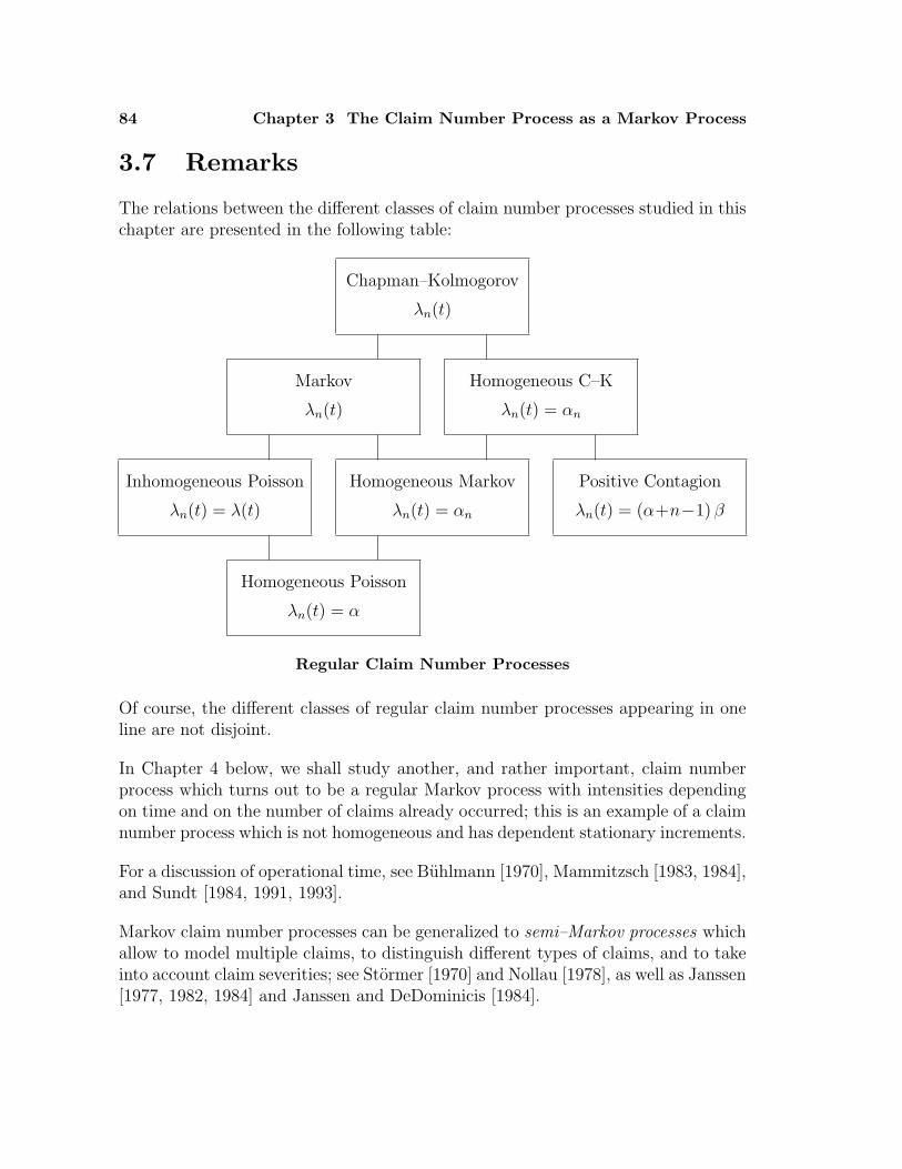
84 Chapter 3 The Claim Number Process as a Markov Process
3.7 Remarks
The relations between the different classes of claim number processes studied in thischapter are presented in the following table:
Chapman–Kolmogorov
λn(t)
Markov
λn(t)
Homogeneous C–K
λn(t) = αn
Inhomogeneous Poisson
λn(t) = λ(t)
Homogeneous Markov
λn(t) = αn
Positive Contagion
λn(t) = (α+n−1) β
Homogeneous Poisson
λn(t) = α
Regular Claim Number Processes
Of course, the different classes of regular claim number processes appearing in oneline are not disjoint.
In Chapter 4 below, we shall study another, and rather important, claim numberprocess which turns out to be a regular Markov process with intensities dependingon time and on the number of claims already occurred; this is an example of a claimnumber process which is not homogeneous and has dependent stationary increments.
For a discussion of operational time, see Buhlmann [1970], Mammitzsch [1983, 1984],and Sundt [1984, 1991, 1993].
Markov claim number processes can be generalized to semi–Markov processes whichallow to model multiple claims, to distinguish different types of claims, and to takeinto account claim severities; see Stormer [1970] and Nollau [1978], as well as Janssen[1977, 1982, 1984] and Janssen and DeDominicis [1984].
Chapter 4
The Mixed Claim NumberProcess
The choice of appropriate assumptions for the claim number process describing aportfolio of risks is a serious problem. In the present chapter we discuss a generalmethod to reduce the problem. The basic idea is to interpret an inhomogeneousportfolio of risks as a mixture of homogeneous portfolios. The claim number processdescribing the inhomogeneous portfolio is then defined to be a mixture of the claimnumber processes describing the homogeneous portfolios such that the mixing distri-bution represents the structure of the inhomogeneous portfolio. We first specify thegeneral model (Section 4.1) and then study the mixed Poisson process (Section 4.2)and, in particular, the Polya–Lundberg process (Section 4.3).
The prerequisites required for the present chapter exceed those for the previous onesin that conditioning will be needed not only in the elementary setting but in fullgenerality. For information on conditioning, see Bauer [1991], Billingsley [1995], andChow and Teicher [1988].
4.1 The Model
Throughout this chapter, let Ntt∈R+be a claim number process and let Θ be a
random variable.
Interpretation: We consider an inhomogeneous portfolio of risks. We assume thatthis inhomogeneous portfolio is a mixture of homogeneous portfolios of the same sizewhich are similar but distinct, and we also assume that each of the homogeneousportfolios can be identified with a realization of the random variable Θ. This meansthat the distribution of Θ represents the structure of the inhomogeneous portfoliounder consideration. The properties of the (unconditional) distribution of the claimnumber process Ntt∈R+
are then determined by the properties of its conditionaldistribution with respect to Θ and by the properties of the distribution of Θ.
86 Chapter 4 The Mixed Claim Number Process
Accordingly, the random variable Θ and its distribution PΘ are said to be the struc-ture parameter and the structure distribution of the portfolio, respectively, and theclaim number process Ntt∈R+
is said to be a mixed claim number process.
The claim number process Ntt∈R+has
– conditionally independent increments with respect to Θ if, for all m ∈ N andt0, t1, . . . , tm ∈ R+ such that 0 = t0 < t1 < . . . < tm, the family of incrementsNtj−Ntj−1
j∈1,...,m is conditionally independent with respect to Θ, and it has– conditionally stationary increments with respect to Θ if, for all m ∈ N and
t0, t1, . . . , tm, h ∈ R+ such that 0 = t0 < t1 < . . . < tm, the family of incrementsNtj+h−Ntj−1+hj∈1,...,m has the same conditional distribution with respect toΘ as Ntj−Ntj−1
j∈1,...,m.It is immediate from the definitions that a claim number process having condition-ally independent increments with respect to Θ has conditionally stationary incre-ments with respect to Θ if and only if the identity PNt+h−Nt|Θ = PNh|Θ holds for allt, h ∈ R+.
4.1.1 Lemma. If the claim number process has conditionally stationary incrementswith respect to Θ, then it has stationary increments.
Proof. For all m∈N and t0, t1, . . . , tm, h ∈ R+ such that 0= t0 <t1 < . . . <tm andfor all k1, . . . , km ∈ N0, we have
P
[m⋂
j=1
Ntj+h−Ntj−1+h = kj]
=
∫
Ω
P
(m⋂
j=1
Ntj+h−Ntj−1+h = kj∣∣∣∣∣ Θ(ω)
)dP (ω)
=
∫
Ω
P
(m⋂
j=1
Ntj−Ntj−1= kj
∣∣∣∣∣ Θ(ω)
)dP (ω)
= P
[m⋂
j=1
Ntj−Ntj−1= kj
],
as was to be shown. 2
By contrast, a claim number process having conditionally independent incrementswith respect to Θ need not have independent increments; see Theorem 4.2.6 below.
The following lemma is immediate from the properties of conditional expectation:
4.1.2 Lemma. If the claim number process Ntt∈R+has finite expectations, then
the identitiesE[Nt] = E[E(Nt|Θ)]
andvar [Nt] = E[var (Nt|Θ)] + var [E(Nt|Θ)]
hold for all t ∈ R+.
The second identity of Lemma 4.1.2 is called the variance decomposition.
4.2 The Mixed Poisson Process 87
4.2 The Mixed Poisson Process
The claim number process Ntt∈R+is a mixed Poisson process with parameter Θ if
Θ is a random variable satisfying PΘ[(0,∞)] = 1 and if Ntt∈R+has conditionally
stationary independent increments with respect to Θ such that PNt|Θ = P(tΘ) holdsfor all t ∈ (0,∞).
We first collect some basic properties of the mixed Poisson process:
4.2.1 Lemma. If the claim number process Ntt∈R+is a mixed Poisson process,
then it has stationary increments and satisfies
P [Nt = n] > 0
for all t ∈ (0,∞) and n ∈ N0.
Proof. By Lemma 4.1.1, the claim number process Ntt∈R+has stationary
increments. Moreover, we have
P [Nt = n] =
∫
Ω
e−tΘ(ω) (tΘ(ω))n
n!dP (ω)
=
∫
Re−tϑ (tϑ)n
n!dPΘ(ϑ) ,
and thus P [Nt = n] > 0. 2
An obvious question to ask is whether or not a mixed Poisson process can haveindependent increments. We shall answer this question at the end of this section.
The following result is a partial generalization of Lemma 2.3.1:
4.2.2 Lemma (Multinomial Criterion). If the claim number process Ntt∈R+
is a mixed Poisson process, then the identity
P
[m⋂
j=1
Ntj−Ntj−1= kj
∣∣∣∣∣Ntm = n]
=n!∏m
j=1 kj!
m∏j=1
(tj−tj−1
tm
)kj
holds for all m ∈ N and t0, t1, . . . , tm ∈ R+ such that 0 = t0 < t1 < . . . < tm andfor all n ∈ N0 and k1, . . . , km ∈ N0 such that
∑mj=1 kj = n.
Proof. We have
P
[m⋂
j=1
Ntj−Ntj−1= kj ∩ Ntm = n
]
= P
[m⋂
j=1
Ntj−Ntj−1= kj
]

88 Chapter 4 The Mixed Claim Number Process
=
∫
Ω
P
(m⋂
j=1
Ntj−Ntj−1= kj
∣∣∣∣∣ Θ(ω)
)dP (ω)
=
∫
Ω
m∏j=1
P (Ntj−Ntj−1= kj|Θ(ω)) dP (ω)
=
∫
Ω
m∏j=1
e−(tj−tj−1)Θ(ω) ((tj−tj−1)Θ(ω))kj
kj!dP (ω)
=n!∏m
j=1 kj!
m∏j=1
(tj−tj−1
tm
)kj
·∫
Ω
e−tmΘ(ω) (tmΘ(ω))n
n!dP (ω)
as well as
P [Ntm = n] =
∫
Ω
e−tmΘ(ω) (tmΘ(ω))n
n!dP (ω) ,
and thus
P
[m⋂
j=1
Ntj−Ntj−1= kj
∣∣∣∣∣ Ntm = n]
=
P
[m⋂
j=1
Ntj−Ntj−1= kj ∩ Ntm = n
]
P [Ntm = n]
=
n!∏mj=1 kj!
m∏j=1
(tj−tj−1
tm
)kj
·∫
Ω
e−tmΘ(ω) (tmΘ(ω))n
n!dP (ω)
∫
Ω
e−tmΘ(ω) (tmΘ(ω))n
n!dP (ω)
=n!∏m
j=1 kj!
m∏j=1
(tj−tj−1
tm
)kj
,
as was to be shown. 2
In the case m = 2, the multinomial criterion is called Lundberg’s binomial criterion.
The multinomial criterion allows to check the assumption that the claim numberprocess is a mixed Poisson process and is useful to compute the finite dimensionaldistributions of a mixed Poisson process.
As a first consequence of the multinomial criterion, we show that every mixed Poissonprocess is a Markov process:
4.2.3 Theorem. If the claim number process is a mixed Poisson process, then itis a Markov process.
4.2 The Mixed Poisson Process 89
Proof. Consider m ∈ N, t1, . . . , tm, tm+1 ∈ (0,∞), and n1, . . . , nm, nm+1 ∈ N0
such that t1 < . . . < tm < tm+1 and P [⋂m
j=1Ntj = nj] > 0. Define t0 := 0 andn0 := 0. Because of the multinomial criterion, we have
P
[Ntm+1 = nm+1
∣∣∣∣∣m⋂
j=1
Ntj = nj]
=
P
[m+1⋂j=1
Ntj = nj]
P
[m⋂
j=1
Ntj = nj]
=
P
[m+1⋂j=1
Ntj−Ntj−1= nj−nj−1
]
P
[m⋂
j=1
Ntj−Ntj−1= nj−nj−1
]
=
P
[m+1⋂j=1
Ntj−Ntj−1= nj−nj−1
∣∣∣∣∣ Ntm+1 = nm+1]· P [Ntm+1 = nm+1]
P
[m⋂
j=1
Ntj−Ntj−1= nj−nj−1
∣∣∣∣∣ Ntm = nm]· P [Ntm = nm]
=
nm+1!∏m+1j=1 (nj−nj−1)!
m+1∏j=1
(tj − tj−1
tm+1
)nj−nj−1
· P [Ntm+1 = nm+1]
nm!∏mj=1(nj−nj−1)!
m∏j=1
(tj − tj−1
tm
)nj−nj−1
· P [Ntm = nm]
=
(nm+1
nm
)(tm
tm+1
)nm(
tm+1 − tmtm+1
)nm+1−nm
· P [Ntm+1 = nm+1]P [Ntm = nm]
as well as
P [Ntm+1 = nm+1|Ntm = nm]= P [Ntm = nm|Ntm+1 = nm+1] ·
P [Ntm+1 = nm+1]P [Ntm = nm]
=
(nm+1
nm
)(tm
tm+1
)nm(
tm+1 − tmtm+1
)nm+1−nm
· P [Ntm+1 = nm+1]P [Ntm = nm] ,
and hence
P
[Ntm+1 = nm+1
∣∣∣∣∣m⋂
j=1
Ntj = nj]
= P [Ntm+1 = nm+1|Ntm = nm] .
This proves the assertion. 2
90 Chapter 4 The Mixed Claim Number Process
4.2.4 Theorem. If the claim number process is a mixed Poisson process withparameter Θ such that Θ has finite moments of any order, then it is regular andsatisfies
pn,n+k(t, t+h) =hk
k!· E[e−(t+h)Θ Θn+k]
E[e−tΘ Θn]
for each admissible pair (n, t) and all k ∈ N0 and h ∈ (0,∞) and with intensitiesλnn∈N satisfying
λn(t) =E[e−tΘ Θn]
E[e−tΘ Θn−1]
for all n ∈ N and t ∈ R+.
Proof. Because of the multinomial criterion, we have
pn,n+k(t, t+h) = P [Nt+h = n + k|Nt = n]= P [Nt = n|Nt+h = n + k] · P [Nt+h = n + k]
P [Nt = n]
=
(n + k
n
)(t
t + h
)n (h
t + h
)k
·
∫
Ω
e(t+h)Θ ((t+h)Θ)n+k
(n+k)!dP
∫
Ω
etΘ (tΘ)n
n!dP
=hk
k!· E[e−(t+h)Θ Θn+k]
E[e−tΘ Θn].
Let us now prove the assertion on regularity.First, Lemma 4.2.1 yields P [Nt = n] > 0, which proves (i).Second, since
pn,n(t, t+h) =E[e−(t+h)Θ Θn]
E[e−tΘ Θn];
the function h 7→ pn,n(t, t+h) is continuous, which proves (ii).Finally, we have
limh→0
1
h
(1− pn,n(t, t+h)
)= lim
h→0
1
h
(1− E[e−(t+h)Θ Θn]
E[e−tΘ Θn]
)
=E[e−tΘ Θn+1]
E[e−tΘ Θn]
as well as
limh→0
1
hpn,n+1(t, t+h) = lim
h→0
1
hh
E[e−(t+h)Θ Θn+1]
E[e−tΘ Θn]
=E[e−tΘ Θn+1]
E[e−tΘ Θn].
This proves (iii).
4.2 The Mixed Poisson Process 91
We have thus shown that Ntt∈R+is regular with intensities λnn∈N satisfying
λn(t) =E[e−tΘ Θn]
E[e−tΘ Θn−1]
for all n ∈ N and t ∈ R+. 2
The following result provides another possibility to check the assumption that theclaim number process is a mixed Poisson process and can be used to estimate theexpectation and the variance of the structure distribution of a mixed Poisson process:
4.2.5 Lemma. If the claim number process Ntt∈R+is a mixed Poisson process
with parameter Θ such that Θ has finite expectation, then the identities
E[Nt] = t E[Θ]
andvar [Nt] = t E[Θ] + t2 var [Θ]
hold for all t∈R+; in particular, the probability of explosion is equal to zero.
Proof. The identities for the moments are immediate from Lemma 4.1.2, and thefinal assertion follows from Corollary 2.1.5. 2
Thus, if the claim number process Ntt∈R+is a mixed Poisson process such that
the structure distribution is nondegenerate and has finite expectation, then, for allt ∈ (0,∞), the variance of Nt strictly exceeds the expectation of Nt; moreover, thevariance of Nt is of order t2 while the expectation of Nt is of order t.
We can now answer the question whether a mixed Poisson process can have inde-pendent increments:
4.2.6 Theorem. If the claim number process Ntt∈R+is a mixed Poisson pro-
cess with parameter Θ such that Θ has finite expectation, then the following areequivalent :(a) The distribution of Θ is degenerate.(b) The claim number process Ntt∈R+
has independent increments.(c) The claim number process Ntt∈R+
is an inhomogeneous Poisson process.(d) The claim number process Ntt∈R+
is a (homogeneous) Poisson process.
Proof. Obviously, (a) implies (d), (d) implies (c), and (c) implies (b).Because of Lemma 4.2.5 and Theorem 2.3.4, (b) implies (d).Assume now that Ntt∈R+
is a Poisson process. Then we have
E[Nt] = var [Nt]
for all t ∈ R+, and Lemma 4.2.5 yields var [Θ] = 0, which means that the structuredistribution is degenerate. Therefore, (d) implies (a). 2
92 Chapter 4 The Mixed Claim Number Process
Problems4.2.A Assume that the claim number process is a mixed Poisson process with parameter
Θ such that Θ has finite moments of any order. Then it has differentiable inten-sities λnn∈N satisfying
λ′n(t)λn(t)
= λn(t)− λn+1(t)
for all n ∈ N and t ∈ R+.
4.2.B Assume that the claim number process is a mixed Poisson process with parameterΘ such that Θ has finite moments of any order. Then the following are equivalent:(a) The intensities are all identical.(b) The intensities are all constant.(c) The claim number process is a homogeneous Poisson process.
4.2.C Estimation: Assume that the claim number process Ntt∈R+is a mixed
Poisson process with parameter Θ such that Θ has a nondegenerate distributionand a finite second moment, and define α = E[Θ]/var [Θ] and γ = E[Θ]2/var [Θ].Then the inequality
E
[(Θ− γ + Nt
α + t
)2]≤ E[(Θ− (a + bNt))2]
holds for all t ∈ R+ and for all a, b ∈ R.
4.2.D Operational Time: If the claim number process is a mixed Poisson process forwhich an operational time exists, then there exist α, γ ∈ (0,∞) such that theintensities satisfy
λn(t) =γ + n− 1
α + t
for all n ∈ N and t ∈ R+.Hint : Use Problems 4.2.A and 3.4.C.
4.2.E Discrete Time Model: The claim number process Nll∈N0is a mixed binomial
process with parameter Θ if PΘ[(0, 1)] = 1 and if Nll∈N0has conditionally
stationary independent increments with respect to Θ such that PNl= B(l, Θ)
holds for all l ∈ N.If the claim number process is a mixed binomial process, then it has stationaryincrements.
4.2.F Discrete Time Model: If the claim number process Nll∈N0is a mixed bino-
mial process, then the identity
P
m⋂
j=1
Nlj−Nlj−1= kj
∣∣∣∣∣∣Nlm = n
=
m∏
j=1
(lj − lj−1
kj
)·(
lmn
)−1
holds for all m ∈ N and l0, l1, . . . , lm ∈ N0 such that 0 = l0 < l1 < . . . < lm andfor all n ∈ N0 and k1, . . . , km ∈ N0 such that kj ≤ lj− lj−1 for all j ∈ 1, . . . , mand such that
∑mj=1 kj = n.
4.3 The Polya–Lundberg Process 93
4.2.G Discrete Time Model: If the claim number process is a mixed binomial pro-cess, then it is a Markov process.
4.2.H Discrete Time Model: If the claim number process Nll∈N0is a mixed bino-
mial process with parameter Θ, then the identities
E[Nl] = l E[Θ]
andvar [Nl] = l E[Θ−Θ2] + l2 var [Θ]
hold for all l ∈ N0.
4.2.I Discrete Time Model: If the claim number process Nll∈N0is a mixed bino-
mial process with parameter Θ, then the following are equivalent:(a) The distribution of Θ is degenerate.(b) The claim number process Nll∈N0
has independent increments.(c) The claim number process Nll∈N0
is a binomial process.
4.2.J Discrete Time Model: Assume that the claim number process Nll∈N0is a
mixed binomial process with parameter Θ such that Θ has a nondegenerate dis-tribution, and define α = E[Θ−Θ2]/var [Θ] and γ = α E[Θ]. Then the inequality
E
[(Θ− γ + Nl
α + l
)2]≤ E[(Θ− (a + bNl))2]
holds for all l ∈ N0 and for all a, b ∈ R.
4.3 The Polya–Lundberg Process
The claim number process Ntt∈R+is a Polya–Lundberg process with parameters
α and γ if it is a mixed Poisson process with parameter Θ such that PΘ = Ga(α, γ).
4.3.1 Theorem. If the claim number process Ntt∈R+is a Polya–Lundberg
process with parameters α and γ, then the identity
P
[m⋂
j=1
Ntj = nj]
=Γ(γ + nm)
Γ(γ)∏m
j=1(nj−nj−1)!
(α
α + tm
)γ m∏j=1
(tj−tj−1
α + tm
)nj−nj−1
holds for all m ∈ N, for all t0, t1, . . . , tm ∈ R+ such that 0 = t0 < t1 < . . . < tm,and for all n0, n1, . . . , nm ∈ N0 such that 0 = n0 ≤ n1 ≤ . . . ≤ nm; in particular, theclaim number process Ntt∈R+
has stationary dependent increments and satisfies
PNt = NB
(γ,
α
α + t
)
for all t ∈ (0,∞) and
PNt+h−Nt|Nt = NB
(γ + Nt,
α + t
α + t + h
)
for all t, h ∈ (0,∞).
94 Chapter 4 The Mixed Claim Number Process
Proof. Because of Lemma 4.2.1 and Theorem 4.2.6, is it clear that the claimnumber process has stationary dependent increments.Let us now prove the remaining assertions:(1) We have
P [Nt = n]
=
∫
Ω
P (Nt = n|Θ(ω)) dP (ω)
=
∫
Ω
e−tΘ(ω) (tΘ(ω))n
n!dP (ω)
=
∫
Re−tϑ (tϑ)n
n!dPΘ(ϑ)
=
∫
Re−tϑ (tϑ)n
n!
αγ
Γ(γ)e−αϑ ϑγ−1 χ(0,∞)(ϑ) dλ(ϑ)
=Γ(γ + n)
Γ(γ) n!
(α
α + t
)γ (t
α + t
)n
·∫
R
(α + t)γ+n
Γ(γ + n)e−(α+t)ϑ ϑγ+n−1 χ(0,∞)(ϑ) dλ(ϑ)
=
(γ + n− 1
n
)(α
α + t
)γ (t
α + t
)n
,
and hence
PNt = NB
(γ,
α
α + t
).
(2) Because of the multinomial criterion and (1), we have
P
[m⋂
j=1
Ntj = nj]
= P
[m⋂
j=1
Ntj = nj∣∣∣∣∣Ntm = nm
]· P [Ntm = nm]
= P
[m⋂
j=1
Ntj−Ntj−1= nj−nj−1
∣∣∣∣∣Ntm = nm]· P [Ntm = nm]
=nm!∏m
j=1(nj−nj−1)!
m∏j=1
(tj−tj−1
tm
)nj−nj−1
·(
γ + nm−1
nm
)(α
α + tm
)γ(tm
α + tm
)nm
=Γ(γ + nm)
Γ(γ)∏m
j=1(nj−nj−1)!
(α
α + tm
)γ m∏j=1
(tj−tj−1
α + tm
)nj−nj−1
.
4.3 The Polya–Lundberg Process 95
(3) Because of (2) and (1), we have
P [Nt+h = n + k ∩ Nt = n]
=Γ(γ + n + k)
Γ(γ) n! k!
(α
α + t + h
)γ (t
α + t + h
)n (h
α + t + h
)k
and
P [Nt = n] =Γ(γ + n)
Γ(γ) n!
(α
α + t
)γ (t
α + t
)n
,
hence
P [Nt+h−Nt = k|Nt = n]
=P [Nt+h−Nt = k ∩ Nt = n]
P [Nt = n]=
P [Nt+h = n+k ∩ Nt = n]P [Nt = n]
=
Γ(γ + n + k)
Γ(γ) n! k!
(α
α + t + h
)γ (t
α + t + h
)n (h
α + t + h
)k
Γ(γ + n)
Γ(γ) n!
(α
α + t
)γ (t
α + t
)n
=
(γ + n + k − 1
k
)(α + t
α + t + h
)γ+n (h
α + t + h
)k
,
and thus
PNt+h−Nt|Nt = NB
(γ + Nt,
α + t
α + t + h
).
This completes the proof. 2
By Theorem 4.3.1, the Polya–Lundberg process is not too difficult to handle sinceits finite dimensional distributions are completely known although its incrementsare not independent.
As an immediate consequence of Theorem 4.3.1, we see that the Polya–Lundbergprocess has positive contagion:
4.3.2 Corollary (Positive Contagion). If the claim number process Ntt∈R+
is a Polya–Lundberg process, then, for all t, h ∈ (0,∞), the function
n 7→ P [Nt+h ≥ n+1|Nt = n]is strictly increasing.
96 Chapter 4 The Mixed Claim Number Process
Thus, for the Polya–Lundberg process, the conditional probability of at least oneclaim occurring in the interval (t, t+h] increases with the number of claims alreadyoccurred up to time t.
We complete the discussion of the Polya–Lundberg process by showing that it is aregular Markov process which is not homogeneous:
4.3.3 Corollary. If the claim number process Ntt∈R+is a Polya–Lundberg
process with parameters α and γ, then it is a regular Markov process satisfying
pn,n+k(t, t+h) =
(γ + n + k − 1
k
)(α + t
α + t + h
)γ+n (h
α + t + h
)k
for each admissible pair (n, t) and all k ∈ N0 and h ∈ R+ and with intensitiesλnn∈N satisfying
λn(t) =γ + n− 1
α + tfor all n ∈ N and t ∈ R+; in particular, the claim number process Ntt∈R+
is nothomogeneous.
Proof. By Theorems 4.2.3 and 4.2.4, the Polya–Lundberg process is a regularMarkov process.By Theorem 4.3.1, we have
pn,n+k(t, t+h) = P [Nt+h = n+k|Nt = n]= P [Nt+h−Nt = k|Nt = n]
=
(γ + n + k − 1
k
)(α + t
α + t + h
)γ+n (h
α + t + h
)k
.
This yields
λn+1(t) = limh→0
1
hpn,n+1(t, t+h)
= limh→0
1
h(γ + n)
(α + t
α + t + h
)γ+nh
α + t + h
=γ + n
α + t,
and thus
λn(t) =γ + n− 1
α + t.
Since the intensities are not constant, it follows from Lemma 3.4.1 that the claimnumber process is not homogeneous. 2
In conclusion, the Polya–Lundberg process is a regular Markov process which isnot homogeneous and has stationary dependent increments. The discussion of thePolya–Lundberg process thus completes the investigation of regular claim numberprocesses satisfying the Chapman–Kolmogorov equations.
4.3 The Polya–Lundberg Process 97
Problems4.3.A Let α, γ ∈ (0,∞). Then the following are equivalent:
(a) The claim number process Ntt∈R+satisfies the Chapman–Kolmogorov
equations and is regular with intensities λnn∈N satisfying
λn(t) =γ + n− 1
α + t
for all n∈N and t∈R+.(b) The identity
pn,n+k(t, t+h) =(
γ + n + k − 1k
) (α + t
α + t + h
)γ+n (h
α + t + h
)k
holds for each admissible pair (n, t) and all k∈N0 and h∈R+.In this case, the claim number process satisfies
PNt = NB(
γ,α
α + t
)
for all t∈(0,∞),
PNt+h−Nt = NB(
γ,α
α + h
)
for all t, h∈(0,∞), and
P [Nt+h−Nt = k|Nt = n] =(
γ + n + k − 1k
)(α + t
α + t + h
)γ+n(h
α + t + h
)k
for all t, h ∈ (0,∞) and all n, k ∈ N0; in particular, the claim number processhas dependent increments and is not homogeneous.Compare the result with Theorem 4.3.1 and Corollary 4.3.3.
4.3.B If the claim number process Ntt∈R+is a Polya–Lundberg process with para-
meters α and γ, thenPW1 = Par(α, γ) .
Try to compute PWn and PTn for arbitrary n ∈ N.
4.3.C Prediction: If the claim number process Ntt∈R+is a Polya–Lundberg process
with parameters α and γ, then the inequality
E
[(Nt+h −
(Nt +
α
α + t· γ
α+
t
α + t· Nt
t
)h
)2]≤ E[(Nt+h − Z)2]
holds for all t, h ∈ (0,∞) and for every random variable Z satisfying E[Z2] < ∞and σ(Z) ⊆ Ft.Interpret the quotient γ/α and compare the result with Theorem 2.3.5.
98 Chapter 4 The Mixed Claim Number Process
4.3.D Prediction: If the claim number process Ntt∈R+is a Polya–Lundberg process
with parameters α and γ, then the identity
E(Nt+h−Nt|Nt) =(
α
α + t· γ
α+
t
α + t· Nt
t
)h
holds for all t, h ∈ (0,∞).Interpret the expression in brackets and compare the result with Problem 4.3.C.
4.3.E Estimation: If the claim number process Ntt∈R+is a Polya–Lundberg process
with parameters α and γ, then the identity
PΘ|Nt= Ga(α + t, γ + Nt)
and henceE(Θ|Nt) =
γ + Nt
α + t
holds for all t ∈ R+.Compare the result with Problems 4.3.D and 4.2.C.
4.3.F Assume that PΘ = Ga(α, γ, δ) with δ ∈ (0,∞). If the claim number processNtt∈R+
is a mixed Poisson process with parameter Θ, then the identity
P
m⋂
j=1
Ntj = nj =
nm!∏mj=1(nj−nj−1)!
·m∏
j=1
(tj−tj−1)nj−nj−1 · e−δtm
(α
α + tm
)γ
·nm∑
k=0
δk
k!
(γ + nm − k − 1
nm − k
)(1
α + tm
)nm−k
holds for all m ∈ N, for all t0, t1, . . . , tm ∈ R+ such that 0 = t0 < t1 < . . . < tmand for all n0, n1, . . . , nm ∈ N0 such that 0 = n0 ≤ n1 ≤ . . . ≤ nm; in particular,the claim number process Ntt∈R+
has stationary dependent increments andsatisfies
PNt = Del(
δt, γ,α
α + t
)
for all t ∈ (0,∞).
4.3.G Assume that PΘ = Ga(α, γ, δ) with δ ∈ (0,∞). If the claim number processNtt∈R+
is a mixed Poisson process with parameter Θ, then it is a regularMarkov process satisfying
pn,n+k(t, t+h) =(
n + k
k
)hk e−δh
(α + t
α + t + h
)γ
·
n+k∑
j=0
δj
j!
(γ + n + k − j − 1
n + k − j
) (1
α + t + h
)n+k−j
n∑
j=0
δj
j!
(γ + n− j − 1
n− j
)(1
α + t + h
)n−j
4.3 The Polya–Lundberg Process 99
for each admissible pair (n, t) and all k ∈ N0 and h ∈ R+ and with intensitiesλnn∈N satisfying
λn(t) = n ·
n∑
j=0
δj
j!
(γ + n− j − 1
n− j
)(1
α + t
)n−j
n−1∑
j=0
δj
j!
(γ + n− 1− j − 1
n− 1− j
)(1
α + t
)n−1−j
for all n ∈ N and t ∈ R+; in particular, the claim number process Ntt∈R+is
not homogeneous.
4.3.H Assume that N ′tt∈R+
and N ′′t t∈R+
are independent claim number processessuch that N ′
tt∈R+is a homogeneous Poisson process with parameter δ and
N ′′t t∈R+
is a Polya–Lundberg process with parameters α and γ. For all t ∈ R+,define
Nt := N ′t + N ′′
t .
Show that Ntt∈R+is a claim number process and compute its finite dimensional
distributions.
4.3.I Discrete Time Model: Assume that PΘ = Be(α, β). If the claim numberprocess Nll∈N0
is a mixed binomial process with parameter Θ, then the identity
P
m⋂
j=1
Nlj = nj =
m∏
j=1
(lj − lj−1
nj − nj−1
)
(lmnm
) ·
(α + nm − 1
nm
)(β + lm − nm − 1
lm − nm
)
(α + β + lm − 1
lm
)
holds for all m ∈ N, for all l0, l1, . . . , lm ∈ N0 such that 0 = l0 < l1 < . . . < lm,and for all n0, n1, . . . , nm ∈ N0 such that 0 = n0 ≤ n1 ≤ . . . ≤ nm and suchthat nj ≤ lj holds for all j ∈ 1, . . . ,m; in particular, the claim number processNll∈N0
has stationary dependent increments and satisfies
PNm = NH(m,α, β)
for all m ∈ N, and
PNm+l−Nm|Nm= NH(l, α+Nm, β+m−Nm)
for all m ∈ N0 and l ∈ N.
4.3.J Discrete Time Model: Assume that PΘ = Be(α, β). If the claim numberprocess Nll∈N0
is a mixed binomial process with parameter Θ, then the identity
PW1 [k] =B(α+1, β+k−1)
B(α, β)
holds for all k ∈ N.Try to compute PWn and PTn for arbitrary n ∈ N.
100 Chapter 4 The Mixed Claim Number Process
4.3.K Discrete Time Model: Assume that PΘ = Be(α, β). If the claim numberprocess Nll∈N0
is a mixed binomial process with parameter Θ, then it is aMarkov process satisfying
pn,n+k(m,m+l) =
(α + n + k − 1
k
)(β + m− n + l − k − 1
l − k
)
(α + β + m + l − 1
l
)
for all m, l ∈ N0, n ∈ 0, 1, . . . ,m and k ∈ 0, 1, . . . ,m + l − n; in particular,the claim number process Nll∈N0
is not homogeneous.
4.3.L Discrete Time Model: Assume that PΘ = Be(α, β). If the claim number pro-cess Nll∈N0
is a mixed binomial process with parameter Θ, then the inequality
E
[(Nm+l −
(Nm +
α+β
α+β+m· E[Θ] +
m
α+β+m· Nm
m
)l
)2]≤ E[(Nm+l−Z)2]
holds for all m, l ∈ N and for every random variable Z satisfying E[Z2] < ∞ andσ(Z) ⊆ Fm.Compare the result with Problem 2.3.F.
4.3.M Discrete Time Model: Assume that PΘ = Be(α, β). If the claim numberprocess Nll∈N0
is a mixed binomial process with parameter Θ, then the identity
E(Nm+l−Nm|Nm) =(
α + β
α + β + m· E[Θ] +
m
α + β + m· Nm
m
)l
holds for all m, l ∈ N.
4.3.N Discrete Time Model: Assume that PΘ = Be(α, β). If the claim numberprocess Nll∈N0
is a mixed binomial process with parameter Θ, then the identity
PΘ|Nm= Be(α + Nm, β + m−Nm)
and henceE(Θ|Nm) =
α + Nm
α + β + m
holds for all m ∈ N0.
4.4 Remarks
The background of the model discussed in this chapter may become clearer if weagree to distinguish between insurer’s portfolios and abstract portfolios. An insurer’sportfolio is, of course, a group of risks insured by the same insurance company; bycontrast, an abstract portfolio is a group of risks which are distributed among one ormore insurance companies. Homogeneous insurer’s portfolios tend to be small, buthomogeneous abstract portfolios may be large. Therefore, it seems to be reasonable
4.4 Remarks 101
to combine information from all insurance companies engaged in the same insurancebusiness in order to model the claim number processes of homogeneous abstractportfolios. This gives reliable information on the conditional distribution of theclaim number process of each insurer’s portfolio. The single insurance company isthen left with the appropriate choice of the structure distribution of its own portfolio.
The interpretation of the mixed claim number process may be extended as follows:Until now, we have assumed that an inhomogeneous insurer’s portfolio is a mixtureof abstract portfolios which are homogeneous. In some classes of nonlife insurancelike industrial fire risks insurance, however, it is difficult to imagine portfolios whichare homogeneous and sufficiently large to provide reliable statistical information. Itis therefore convenient to modify the model by assuming that a rather inhomoge-neous insurer’s portfolio is a mixture of rather homogeneous abstract portfolios – themathematics of mixing does not change at all. Once this generalization is accepted,we may also admit more than two levels of inhomogeneity and mix rather homoge-neous portfolios to describe more and more inhomogeneous portfolios. In any case,the level of inhomogeneity of a portfolio is reflected by the variance of the structuredistribution, which is equal to zero if and only if the portfolio is homogeneous.
There is still another variant of the interpretations given so far: The mixed claimnumber process may interpreted as the claim number process of a single risk selectedat random from an inhomogeneous portfolio of risks which are similar but distinctand which can be characterized by a realization of the structure parameter which isnot observable. This interpretation provides a link between claim number processesor aggregate claims processes and experience rating – a theory of premium calculationwhich, at its core, is concerned with optimal prediction of future claim numbers orclaim severities of single risks, given individual claims experience in the past as wellas complete or partial information on the structure of the portfolio from which therisk was selected. An example of an optimal prediction formula for future claimnumbers is given in Problem 4.3.C. For an introduction to experience rating, seeSundt [1984, 1991, 1993] and Schmidt [1992].
According to Seal [1983], the history of the mixed Poisson process dates back toa paper of Dubourdieu [1938] who proposed it as a model in automobile insurancebut did not compare the model with statistical data. Two years later, the mixedPoisson process became a central topic in the famous book by Lundberg [1940]who developed its mathematical theory and studied its application to sickness andaccident insurance. Still another application was suggested by Hofmann [1955] whostudied the mixed Poisson process as a model for workmen’s compensation insurance.
For further details on the mixed Poisson process, it is worth reading Lundberg[1940]; see also Albrecht [1981], the surveys by Albrecht [1985] and Pfeifer [1986],and the recent manuscript by Grandell [1995]. Pfeifer [1982a, 1982b] and Gerber[1983] studied asymptotic properties of the claim arrival process induced by a Polya–Lundberg process, and Pfeifer and Heller [1987] and Pfeifer [1987] characterized the
102 Chapter 4 The Mixed Claim Number Process
mixed Poisson process in terms of the martingale property of certain transforms ofthe claim arrival process. The mixed Poisson process with a structure parameterhaving a three–parameter Gamma distribution was first considered by Delaporte[1960, 1965], and further structure distributions were discussed by Troblinger [1961],Kupper [1962], Albrecht [1981], and Gerber [1991]. These authors, however, studiedonly the one–dimensional distributions of the resulting claim number processes.
In order to select a claim number process as a model for given data, it is useful torecall some criteria which are fulfilled for certain claim number processes but fail forothers. The following criteria refer to the inhomogeneous Poisson process and themixed Poisson process, each of them including the homogeneous Poisson process asa special case:– Independent increments : The inhomogeneous Poisson process has independent
increments, but the mixed Poisson process with a nondegenerate structure dis-tribution has not.
– Stationary increments : The mixed Poisson process has stationary increments,but the inhomogeneous Poisson process with a nonconstant intensity has not.
– Multinomial criterion: The multinomial criterion with probabilities propertionalto time intervals holds for the mixed Poisson process, but it fails for the inhomo-geneous Poisson process with a nonconstant intensity.
– Moment inequality : The moment inequality,
E[Nt] ≤ var [Nt]
for all t ∈ (0,∞), is a strict inequality for the mixed Poisson process with anondegenerate structure distribution, but it is an equality for the inhomogeneousPoisson process.
Once the type of the claim number process has been selected according to theprevious criteria, the next step should be to choose parameters and to examine thegoodness of fit of the theoretical finite dimensional distributions to the empiricalones.
Automobile insurance was not only the godfather of the mixed Poisson process whenit was introduced in risk theory by Dubourdieu [1938] without reference to statisticaldata; it still is the most important class of insurance in which the mixed Poissonprocess seems to be a good model for the empirical claim number process. This isindicated in the papers by Thyrion [1960], Delaporte [1960, 1965], Troblinger [1961],Derron [1962], Bichsel [1964], and Ruohonen [1988], and in the book by Lemaire[1985]. As a rule, however, these authors considered data from a single period onlyand hence compared one–dimensional theoretical distributions with empirical ones.In order to model the development of claim numbers in time, it would be necessaryto compare the finite dimensional distributions of selected claim number processeswith those of empirical processes.
Chapter 5
The Aggregate Claims Process
In the present chapter we introduce and study the aggregate claims process. We firstextend the model considered so far (Section 5.1) and then establish some generalresults on compound distributions (Section 5.2). It turns out that aggregate claimsdistributions can be determined explicitly only in a few exceptional cases. However,the most important claim number distributions can be characterized by a simplerecursion formula (Section 5.3) and admit the recursive computation of aggregateclaims distributions and their moments when the claim size distribution is discrete(Section 5.4).
5.1 The Model
Throughout this chapter, let Ntt∈R+be a claim number process and let Tnn∈N0
be the claim arrival process induced by the claim number process. We assume thatthe exceptional null set is empty and that the probability of explosion is equal tozero.
Furthermore, let Xnn∈N be a sequence of random variables. For t ∈ R+, define
St :=Nt∑
k=1
Xk
=∞∑
n=0
χNt=nn∑
k=1
Xk .
Of course, we have S0 = 0.
Interpretation:– Xn is the claim amount or claim severity or claim size of the nth claim.– St is the aggregate claims amount of the claims occurring up to time t.Accordingly, the sequence Xnn∈N is said to be the claim size process, and thefamily Stt∈R+
is said to be the aggregate claims process induced by the claimnumber process and the claim size process.
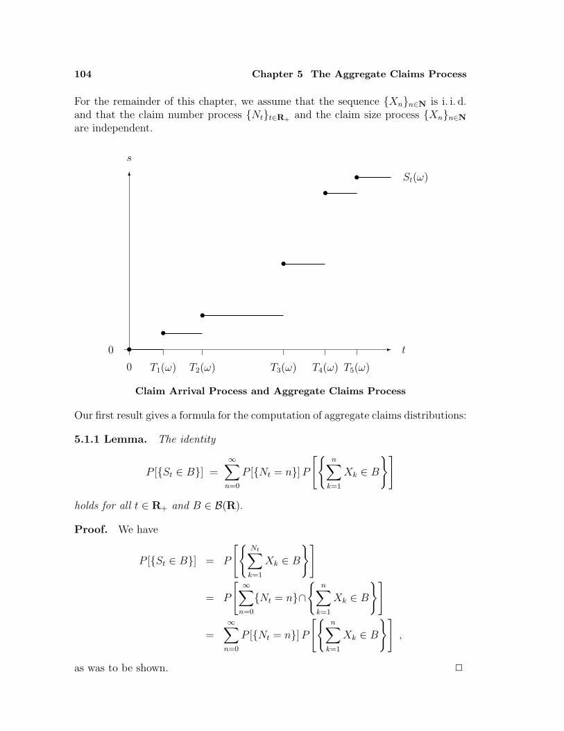
104 Chapter 5 The Aggregate Claims Process
For the remainder of this chapter, we assume that the sequence Xnn∈N is i. i. d.and that the claim number process Ntt∈R+
and the claim size process Xnn∈Nare independent.
0 -
s
6
0 T1(ω) T2(ω) T3(ω) T4(ω) T5(ω)
t••
•
•
•• St(ω)
Claim Arrival Process and Aggregate Claims Process
Our first result gives a formula for the computation of aggregate claims distributions:
5.1.1 Lemma. The identity
P [St ∈ B] =∞∑
n=0
P [Nt = n] P[
n∑
k=1
Xk ∈ B
]
holds for all t ∈ R+ and B ∈ B(R).
Proof. We have
P [St ∈ B] = P
[Nt∑
k=1
Xk ∈ B
]
= P
[ ∞∑n=0
Nt = n∩
n∑
k=1
Xk ∈ B
]
=∞∑
n=0
P [Nt = n] P[
n∑
k=1
Xk ∈ B
],
as was to be shown. 2
5.1 The Model 105
For s, t ∈ R+ such that s ≤ t, the increment of the aggregate claims processStt∈R+
on the interval (s, t] is defined to be
St − Ss :=Nt∑
k=Ns+1
Xk .
Since S0 = 0, this is in accordance the definition of St; in addition, we have
St(ω) = (St−Ss)(ω) + Ss(ω) ,
even if Ss(ω) is infinite. For the aggregate claims process, the properties of havingindependent or stationary increments are defined in the same way as for the claimnumber process.
5.1.2 Theorem. If the claim number process has independent increments, thenthe same is true for the aggregate claims process.
Proof. Consider m ∈ N, t0, t1, . . . , tm ∈ R+ such that 0 = t0 < t1 < . . . < tm, andB1, . . . , Bm ∈ B(R). For all n0, n1, . . . , nm ∈ N0 such that 0 = n0 ≤ n1 ≤ . . . ≤ nm,we have
P
[(m⋂
j=1
Ntj = nj
)∩
(m⋂
j=1
nj∑
k=nj−1+1
Xk ∈ Bj
)]
= P
[m⋂
j=1
Ntj = nj
]· P
[m⋂
j=1
nj∑
k=nj−1+1
Xk ∈ Bj
]
= P
[m⋂
j=1
Ntj−Ntj−1= nj−nj−1
]· P
[m⋂
j=1
nj∑
k=nj−1+1
Xk ∈ Bj
]
=m∏
j=1
P [Ntj−Ntj−1= nj−nj−1] ·
m∏j=1
P
[nj∑
k=nj−1+1
Xk ∈ Bj
]
=m∏
j=1
(P [Ntj−Ntj−1
= nj−nj−1] P
[nj−nj−1∑
k=1
Xk ∈ Bj
]).
This yields
P
[m⋂
j=1
Stj−Stj−1
∈ Bj
]
= P
[m⋂
j=1
Ntj∑
k=Ntj−1+1
Xk ∈ Bj
]
106 Chapter 5 The Aggregate Claims Process
= P
[ ∞∑n1=0
∞∑n2=n1
· · ·∞∑
nm=nm−1
(m⋂
j=1
Ntj = nj
)∩
(m⋂
j=1
Nj∑
k=Nj−1+1
Xk ∈ Bj
)]
=∞∑
n1=0
∞∑n2=n1
· · ·∞∑
nm=nm−1
P
[(m⋂
j=1
Ntj = nj
)∩
(m⋂
j=1
nj∑
k=nj−1+1
Xk ∈ Bj
)]
=∞∑
n1=0
∞∑n2=n1
· · ·∞∑
nm=nm−1
m∏j=1
(P [Ntj−Ntj−1
= nj−nj−1] P
[nj−nj−1∑
k=1
Xk ∈ Bj
])
=∞∑
l1=0
∞∑
l2=0
· · ·∞∑
lm=0
m∏j=1
(P [Ntj−Ntj−1
= lj] P
[lj∑
k=1
Xk ∈ Bj
])
=m∏
j=1
( ∞∑
lj=0
P [Ntj−Ntj−1= lj] P
[lj∑
k=1
Xk ∈ Bj
]).
The assertion follows. 2
5.1.3 Theorem. If the claim number process has stationary independent incre-ments, then the same is true for the aggregate claims process.
Proof. By Theorem 5.1.2, the aggregate claims process has independent incre-ments.Consider t, h ∈ R+. For all B ∈ B(R), Lemma 5.1.1 yields
P[
St+h−St ∈ B]
= P
[Nt+h∑
k=Nt+1
Xk ∈ B
]
= P
[ ∞∑n=0
∞∑m=0
Nt = n∩Nt+h−Nt = m∩
n+m∑
k=n+1
Xk ∈ B
]
=∞∑
n=0
∞∑m=0
P [Nt = n] P [Nt+h−Nt = m] P[
n+m∑
k=n+1
Xk ∈ B
]
=∞∑
n=0
P [Nt = n]∞∑
m=0
P [Nh = m] P[
m∑
k=1
Xk ∈ B
]
=∞∑
m=0
P [Nh = m] P[
m∑
k=1
Xk ∈ B
]
= P [Sh ∈ B] .
Therefore, the aggregate claims process has also stationary increments. 2
5.1 The Model 107
The assumption of Theorem 5.1.3 is fulfilled when the claim number process isa Poisson process; in this case, the aggregate claims process is also said to be acompound Poisson process.
Interpretation: For certain claim size distributions, the present model admitsinterpretations which differ from the one presented before. Of course, if the claimsize distribution satisfies PX [1] = 1, then the aggregate claims process is identicalwith the claim number process. More generally, if the claim size distribution satisfiesPX [N] = 1, then the following interpretation is possible:– Nt is the number of claim events up to time t,– Xn is the number of claims occurring at the nth claim event, and– St is the total number of claims up to time t.This shows the possibility of applying our model to an insurance business in whichtwo or more claims may occur simultaneously.
Further interesting interpretations are possible when the claim size distribution is aBernoulli distribution:
5.1.4 Theorem (Thinned Claim Number Process). If the claim size dis-tribution is a Bernoulli distribution, then the aggregate claims process is a claimnumber process.
Proof. Since PX is a Bernoulli distribution, there exists a null set ΩX ∈ F suchthat
Xn(ω) ∈ 0, 1
holds for all n ∈ N and ω ∈ Ω\ΩX . Furthermore, since E[X] > 0, the Chung–Fuchstheorem yields the existence of a null set Ω∞ ∈ F such that
∞∑n=1
Xk(ω) = ∞
holds for all ω ∈ Ω \ Ω∞. Define
ΩS := ΩX ∪ Ω∞ .
It now follows from the properties of the claim number process Ntt∈R+and the
previous remarks that the aggregate claims process Stt∈R+is a claim number
process with exceptional null set ΩS. 2
Comment: Thinned claim number processes occur in the following situations:– Assume that PX = B(η). If η is interpreted as the probability for a claim to
be reported, then Nt is the number of occurred claims and St is the number ofreported claims, up to time t.
108 Chapter 5 The Aggregate Claims Process
– Consider a sequence of random variables Ynn∈N which is i. i. d. and assumethat Ntt∈R+
and Ynn∈N are independent. Consider also c ∈ (0,∞) andassume that η := P [Y > c] ∈ (0, 1). Then the sequence Xnn∈N, given byXn := χYn>c, is i. i. d. such that PX = B(η), and Ntt∈R+
and Xnn∈N areindependent. If Yn is interpreted as the size of the nth claim, then Nt is thenumber of occurred claims and St is the number of large claims (exceeding c),up to time t. This is of interest in excess of loss reinsurance, or XL reinsurancefor short, where the reinsurer assumes responsibility for claims exceeding thepriority c.
A particularly interesting result on thinned claim number processes is the following:
5.1.5 Corollary (Thinned Poisson Process). If the claim number process isa Poisson process with parameter α and if the claim size distribution is a Bernoullidistribution with parameter η, then the aggregate claims process is a Poisson processwith parameter αη.
Proof. By Theorem 5.1.3, the aggregate claims process has stationary independentincrements.Consider t ∈ (0,∞). By Lemma 5.1.1, we have
P [St = m] =∞∑
n=0
P [Nt = n] P[
n∑
k=1
Xk = m
]
=∞∑
n=m
e−αt (αt)n
n!
(n
m
)ηm(1−η)n−m
=∞∑
n=m
e−αηt (αηt)m
m!e−α(1−η)t (α(1−η)t)n−m
(n−m)!
= e−αηt (αηt)m
m!
∞∑j=0
e−α(1−η)t (α(1−η)t)j
j!
= e−αηt (αηt)m
m!
for all m ∈ N0, and hence PSt = P(αηt).Therefore, the aggregate claims process is a Poisson process with parameter αη. 2
We shall return to the thinned claim number process in Chapter 6 below.
Problem5.1.A Discrete Time Model (Thinned Binomial Process): If the claim number
process is a binomial process with parameter ϑ and if the claim size distributionis a Bernoulli distribution with parameter η, then the aggregate claims processis a binomial process with parameter ϑη.
5.2 Compound Distributions 109
5.2 Compound Distributions
In this and the following sections of the present chapter we shall study the problemof computing the distribution of the aggregate claims amount St at a fixed time t.To this end, we simplify the notation as follows:
Let N be a random variable satisfying PN [N0] = 1 and define
S :=N∑
k=1
Xk .
Again, the random variables N and S will be referred to as the claim number andthe aggregate claims amount, respectively.
We assume throughout that N and Xnn∈N are independent, and we maintainthe assumption made before that the sequence Xnn∈N is i. i. d. In this case, theaggregate claims distribution PS is said to be a compound distribution and is denotedby
C(PN , PX) .
Compound distributions are also named after the claim number distribution; forexample, if PN is a Poisson distribution, then C(PN , PX) is said to be a compoundPoisson distribution.
The following result is a reformulation of Lemma 5.1.1:
5.2.1 Lemma. The identity
PS[B] =∞∑
n=0
PN [n] P ∗nX [B]
holds for all B ∈ B(R).
Although this formula is useful in certain special cases, it requires the computa-tion of convolutions which may be difficult or at least time consuming. For themost important claim number distributions and for claim size distributions satis-fying PX [N0] = 1, recursion formulas for the aggregate claims distribution and itsmoments will be given in Section 5.4 below.
In some cases, it is also helpful to look at the characteristic function of the aggregateclaims distribution.
5.2.2 Lemma. The characteristic function of S satisfies
ϕS(z) = mN(ϕX(z)) .
110 Chapter 5 The Aggregate Claims Process
Proof. For all z ∈ R, we have
ϕS(z) = E[eizS
]
= E[eiz
∑N
k=1Xk
]
= E
[ ∞∑n=0
χN=neiz
∑n
k=1Xk
]
= E
[ ∞∑n=0
χN=nn∏
k=1
eizXk
]
=∞∑
n=0
P [N = n]n∏
k=1
E[eizXk
]
=∞∑
n=0
P [N = n] E[eizX
]n
=∞∑
n=0
P [N = n] ϕX(z)n
= E[ϕX(z)N
]
= mN(ϕX(z)) ,
as was to be shown. 2
To illustrate the previous result, let us consider some applications.
Let us first consider the compound Poisson distribution.
5.2.3 Corollary. If PN = P(α), then the characteristic function of S satisfies
ϕS(z) = eα(ϕX(z)−1) .
If the claim number distribution is either a Bernoulli distribution or a logarithmicdistribution, then the computation of the compound Poisson distribution can besimplified as follows:
5.2.4 Corollary. For all α ∈ (0,∞) and η ∈ (0, 1),
C(P(α),B(η)
)= P(αη) .
5.2.5 Corollary. For all α ∈ (0,∞) and η ∈ (0, 1),
C(P(α),Log(η)
)= NB
(α
| log(1−η)| , 1−η
).
5.2 Compound Distributions 111
Thus, the compound Poisson distributions of Corollaries 5.2.4 and 5.2.5 are nothingelse than a Poisson or a negativebinomial distribution, which are easily computedby recursion; see Theorem 5.3.1 below.
Let us now consider the compound negativebinomial distribution.
5.2.6 Corollary. If PN = NB(α, ϑ), then the characteristic function of S satisfies
ϕS(z) =
(ϑ
1− (1−ϑ)ϕX(z)
)α
.
A result analogous to Corollary 5.2.4 is the following:
5.2.7 Corollary. For all α ∈ (0,∞) and ϑ, η ∈ (0, 1),
C(NB(α, ϑ),B(η)
)= NB
(α,
ϑ
ϑ + (1−ϑ)η
).
For the compound negativebinomial distribution, we have two further results:
5.2.8 Corollary. For all m ∈ N, ϑ ∈ (0, 1), and β ∈ (0,∞),
C(NB(m,ϑ),Exp(β)
)= C
(B(m, 1−ϑ),Exp(βϑ)
).
5.2.9 Corollary. For all m ∈ N and ϑ, η ∈ (0, 1),
C(NB(m,ϑ),Geo(η)
)= C
(B(m, 1−ϑ),Geo(ηϑ)
).
Corollaries 5.2.8 and 5.2.9 are of interest since the compound binomial distributionis determined by a finite sum.
Let us now turn to the discussion of moments of the aggregate claims distribution:
5.2.10 Lemma (Wald’s Identities). Assume that E[N ] < ∞ and E|X| < ∞.Then the expectation and the variance of S exist and satisfy
E[S] = E[N ] E[X]
and
var [S] = E[N ] var [X] + var [N ] E[X]2 .
112 Chapter 5 The Aggregate Claims Process
Proof. We have
E[S]
= E
[N∑
k=1
Xk
]
= E
[ ∞∑n=1
χN=nn∑
k=1
Xk
]
=∞∑
n=1
P [N = n] E[
n∑
k=1
Xk
]
=∞∑
n=1
P [N = n] nE[X]
= E[N ] E[X] ,
which is the first identity.Similarly, we have
E[S2
]= E
(
N∑
k=1
Xk
)2
= E
∞∑n=1
χN=n
(n∑
k=1
Xk
)2
=∞∑
n=1
P [N = n] E(
n∑
k=1
Xk
)2
=∞∑
n=1
P [N = n]var
[n∑
k=1
Xk
]+
(E
[n∑
k=1
Xk
])2
=∞∑
n=1
P [N = n](n var [X] + n2 E[X]2
)
= E[N ] var [X] + E[N2] E[X]2 ,
and thus
var [S] = E[S2]− E[S]2
=(E[N ] var [X] + E[N2] E[X]2
)−
(E[N ] E[X]
)2
= E[N ] var [X] + var [N ] E[X]2 ,
which is the second identity. 2
5.2 Compound Distributions 113
5.2.11 Corollary. Assume that PN = P(α) and E|X| < ∞. Then
E[S] = α E[X]
andvar [S] = α E[X2] .
The following general inequalities provide upper bounds for the tail probabilitiesP [S ≥ c] of the aggregate claims distribution:
5.2.12 Lemma. Let Z be a random variable and let h : R → R+ be a measurablefunction which is strictly increasing on R+. Then the inequality
P [Z ≥ c] ≤ E[h(|Z|)]h(c)
holds for all c ∈ (0,∞).
Proof. By Markov’s inequality, we have
P [Z ≥ c] ≤ P [|Z| ≥ c]= P [h(|Z|) ≥ h(c)]
≤ E[h(|Z|)]h(c)
,
as was to be shown. 2
5.2.13 Lemma (Cantelli’s Inequality). Let Z be a random variable satisfyingE[Z2] < ∞. Then the inequality
P [Z ≥ E[Z] + c] ≤ var [Z]
c2 + var [Z]
holds for all c ∈ (0,∞).
Proof. Define Y := Z −E[Z]. Then we have E[Y ] = 0 and var [Y ] = var [Z]. Forall x ∈ (−c,∞), Lemma 5.2.12 yields
P[Z ≥ E[Z] + c] = P
[Y ≥ c]
= P[Y + x ≥ c + x]
≤ E[(Y + x)2
]
(c + x)2
=E[Y 2] + x2
(c + x)2
=var [Y ] + x2
(c + x)2
=var [Z] + x2
(c + x)2.
114 Chapter 5 The Aggregate Claims Process
The last expression attains its minimum at x = var [Z]/c, and this yields
P[Z ≥ E[Z] + c] ≤
var [Z] +
(var [Z]
c
)2
(c +
var [Z]
c
)2
=c2 var [Z] +
(var [Z]
)2
(c2 + var [Z]
)2
=var [Z]
c2 + var [Z],
as was to be shown. 2
Problems5.2.A Let Q denote the collection of all distributions Q : B(R) → [0, 1] satisfying
Q[N0] = 1. For Q, R ∈ Q, define C(Q,R) by letting
C(Q, R)[B] :=∞∑
n=0
Q[n] R∗n[B]
for all B ∈ B(R). Then C(Q,R) ∈ Q. Moreover, the map C : Q×Q → Q turnsQ into a noncommutative semigroup with neutral element δ1.
5.2.B Ammeter Transform: For all α ∈ (0,∞) and ϑ ∈ (0, 1),
C(NB(α, ϑ), PX
)= C
(P(α |log(ϑ)|),C(Log(1−ϑ), PX)
).
5.2.C Discrete Time Model: For all m ∈ N and ϑ, η ∈ (0, 1),
C(B(m,ϑ),B(η)
)= B(m,ϑη) .
5.2.D Discrete Time Model: For all m ∈ N, ϑ ∈ (0, 1), and β ∈ (0,∞),
C(B(m,ϑ),Exp(β)
)=
m∑
k=0
(m
k
)ϑk(1−ϑ)m−k Ga(β, k) ,
where Ga(β, 0) := δ0. Combine the result with Corollary 5.2.8.
5.2.E If E[N ] < ∞ and E|X| < ∞, then
minE[N ], var [N ] · E[X2] ≤ var [S] ≤ maxE[N ], var [N ] · E[X2] .
If PN = P(α), then these lower and upper bounds for var [S] are identical.
5.2.F If E[N ] ∈ (0,∞), PX [R+] = 1 and E[X] ∈ (0,∞), then
v2[S] = v2[N ] +1
E[N ]v2[X] .
5.2.G If PN = P(α), PX [R+] = 1 and E[X] ∈ (0,∞), then
v2[S] =1α
(1 + v2[X]
).
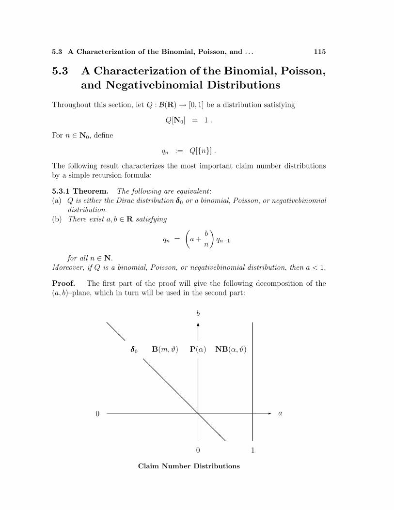
5.3 A Characterization of the Binomial, Poisson, and . . . 115
5.3 A Characterization of the Binomial, Poisson,and Negativebinomial Distributions
Throughout this section, let Q : B(R) → [0, 1] be a distribution satisfying
Q[N0] = 1 .
For n ∈ N0, define
qn := Q[n] .
The following result characterizes the most important claim number distributionsby a simple recursion formula:
5.3.1 Theorem. The following are equivalent :(a) Q is either the Dirac distribution δ0 or a binomial, Poisson, or negativebinomial
distribution.(b) There exist a, b ∈ R satisfying
qn =
(a +
b
n
)qn−1
for all n ∈ N.Moreover, if Q is a binomial, Poisson, or negativebinomial distribution, then a < 1.
Proof. The first part of the proof will give the following decomposition of the(a, b)–plane, which in turn will be used in the second part:
0 - a
@@@
@@@@@@@@@@@@@
b
6
0 1
δ0 B(m,ϑ) P(α) NB(α, ϑ)
Claim Number Distributions
116 Chapter 5 The Aggregate Claims Process
• Assume first that (a) holds.If Q=δ0, then the recursion holds with a = b = 0.If Q=B(m,ϑ), then the recursion holds with a = −ϑ/(1−ϑ) and b = (m+1) ϑ/(1−ϑ).If Q=P(α), then the recursion holds with a = 0 and b = α.If Q=NB(α, ϑ), then the recursion holds with a = 1−ϑ and b = (α−1)(1−ϑ).Therefore, (a) implies (b).• Assume now that (b) holds. The assumption implies that q0 > 0.Assume first that q0 = 1. Then we have
Q = δ0 .
Assume now that q0 < 1. Then we have 0 < q1 = (a + b) q0, and thus
a + b > 0 .
The preceding part of the proof suggests to distinguish the three cases a < 0, a = 0,and a > 0.(1) The case a < 0 : Since a+ b > 0, we have b > 0, and it follows that the sequencea + b/nn∈N decreases to a. Therefore, there exists some m ∈ N satisfying qm > 0and qm+1 = 0, hence 0 = qm+1 = (a + b/(m+1)) qm, and thus a + b/(m+1) = 0.This yields
m =a + b
−a
and b = (m+1)(−a). For all n ∈ 1, . . . ,m, this gives
qn =
(a +
b
n
)qn−1
=
(a +
(m+1)(−a)
n
)qn−1
=m + 1− n
n(−a) qn−1 ,
and thus
qn =
(n∏
k=1
m + 1− k
k
)(−a)n q0
=
(m
n
)(−a)n q0 .
Summation gives
1 =m∑
n=0
qn
=m∑
n=0
(m
n
)(−a)n q0
= (1− a)m q0 ,
5.3 A Characterization of the Binomial, Poisson, and . . . 117
hence q0 = (1− a)−m, and thus
qn =
(m
n
)(−a)n q0
=
(m
n
)(−a)n (1− a)−m
=
(m
n
)( −a
1− a
)n(1
1− a
)m−n
for all n ∈ 0, . . . ,m. Therefore, we have
Q = B
(a + b
−a,−a
1− a
).
(2) The case a = 0 : Since a + b > 0, we have b > 0. For all n ∈ N, we have
qn =b
nqn−1 ,
and thus
qn =bn
n!q0 .
Summation gives
1 =∞∑
n=0
qn
=∞∑
n=0
bn
n!q0 ,
hence q0 = e−b, and thus
qn = e−b bn
n!
for all n ∈ N0. Therefore, we have
Q = P(b) .
(3) The case a > 0 : Define c := (a+b)/a. Then we have c > 0 and b = (c−1) a. Forall n ∈ N, this gives
qn =
(a +
b
n
)qn−1
=
(a +
(c−1)a
n
)qn−1
=c + n− 1
na qn−1 ,
118 Chapter 5 The Aggregate Claims Process
and thus
qn =
(n∏
k=1
c + k − 1
k
)anq0
=
(c + n− 1
n
)anq0 .
In particular, we have qn ≥ (1/n)canq0. Since∑∞
n=0 qn = 1, we must have a < 1.Summation yields
1 =∞∑
n=0
qn
=∞∑
n=0
(c + n− 1
n
)anq0
= (1− a)−c q0 ,
hence q0 = (1− a)c, and thus
qn =
(c + n− 1
n
)anq0
=
(c + n− 1
n
)(1− a)c an .
Therefore, we have
Q = NB
(a + b
a, 1− a
).
We have thus shown that (b) implies (a).• The final assertion has already been shown in the preceding part of the proof. 2
Theorem 5.3.1 and its proof suggest to consider the family of all distributions Qsatisfying Q[N0] = 1 and for which there exist a, b ∈ R satisfying −b < a < 1 and
qn =
(a +
b
n
)qn−1
for all n ∈ N as a parametric family of distributions which consists of the binomial,Poisson, and negativebinomial distributions. Note that the Dirac distribution δ0 isexcluded since it does not determine the parameters uniquely.
5.4 The Recursions of Panjer and DePril 119
Problems5.3.A Let Q be a nondegenerate distribution satisfying Q[N0] = 1 and
qn =(
a +b
n
)qn−1
for suitable a, b ∈ R and all n ∈ N. Then the expectation and the variance of Qexist and satisfy
E[Q] =a + b
1− a
andvar [Q] =
a + b
(1− a)2,
and hencevar [Q]E[Q]
=1
1− a.
Interpret this last identity with regard to Theorem 5.3.1 and its proof, and illus-trate the result in the (a, b)–plane. Show also that
v2[Q] =1
a + b.
and interpret the result.
5.3.B If Q is a geometric or logarithmic distribution, then there exist a, b ∈ R satisfying
qn =(
a +b
n
)qn−1
for all n ∈ N such that n ≥ 2.
5.3.C If Q is a Delaporte distribution, then there exist a1, b1, b2 ∈ R satisfying
qn =(
a1 +b1
n
)qn−1 +
b2
nqn−2
for all n ∈ N such that n ≥ 2.
5.3.D If Q is a negativehypergeometric distribution, then there exist c0, c1, d0, d1 ∈ Rsatisfying
qn =c0 + c1n
d0 + d1nqn−1
for all n ∈ N.
5.4 The Recursions of Panjer and DePril
The aim of this section is to prove that the recursion formula for the binomial,Poisson, and negativebinomial distributions translates into recursion formulas forthe aggregate claims distribution and its momemts when the claim size distributionis concentrated on N0.
120 Chapter 5 The Aggregate Claims Process
Throughout this section, we assume that
PX [N0] = 1 .
Then we have PS[N0] = 1.
Comment: At the first glance, it may seem a bit confusing to assume PX [N0] = 1instead of PX [N] = 1. Indeed, claim severities should be strictly positive, and this isalso true for the number of claims at a claim event. However, our assumption allowsPX to be an aggregate claims distribution, and this opens the possibility of applyingPanjer’s recursion repeatedly for a class of claim number distributions which arecompound distributions; see Problem 5.4.D below.
For all n ∈ N0, define
pn := P [N = n]fn := P [X = n]gn := P [S = n] .
Then the identity of Lemma 5.2.1 can be written as
gn =∞∑
k=0
pk f ∗kn .
Note that the sum occurring in this formula actually extends only over a finitenumber of terms.
5.4.1 Lemma. The identities
f ∗nm =m∑
k=0
f∗(n−1)m−k fk
and
f ∗nm =n
m
m∑
k=1
k f∗(n−1)m−k fk
hold for all n,m ∈ N.
Proof. For all j ∈ 1, . . . , n and k ∈ 0, 1, . . . ,m, we have
P
[n∑
i=1
Xi = m
∩Xj = k
]= P
[n∑
j 6=i=1
Xi = m−k
∩Xj = k
]
= P
[n∑
j 6=i=1
Xi = m−k
]· P [Xj = k]
= f∗(n−1)m−k fk .
5.4 The Recursions of Panjer and DePril 121
This yields
f ∗nm = P
[n∑
i=1
Xi = m
]
=m∑
k=0
P
[n∑
i=1
Xi = m
∩Xj = k
]
=m∑
k=0
f∗(n−1)m−k fk ,
which is the first identity, as well as
E
[χ∑n
i=1Xi=mXj
]=
m∑
k=0
E
[χ∑n
i=1Xi=m∩Xj=kXj
]
=m∑
k=1
E
[χ∑n
i=1Xi=m∩Xj=kk
]
=m∑
k=1
k P
[n∑
i=1
Xi = m
∩Xj = k
]
=m∑
k=1
k f∗(n−1)m−k fk
for all j ∈ 1, . . . , n, and hence
f ∗nm = P
[n∑
i=1
Xi = m
]
= E
[χ∑n
i=1Xi=m
]
= E
[χ∑n
i=1Xi=m
1
m
n∑j=1
Xj
]
=1
m
n∑j=1
E
[χ∑n
i=1Xi=mXj
]
=1
m
n∑j=1
m∑
k=1
k f∗(n−1)m−k fk
=n
m
m∑
k=1
k f∗(n−1)m−k fk ,
which is the second identity. 2
122 Chapter 5 The Aggregate Claims Process
For the nondegenerate claim number distributions characterized by Theorem 5.3.1,we can now prove a recursion formula for the aggregate claims distribution:
5.4.2 Theorem (Panjer’s Recursion). If the distribution of N is nondegenerateand satisfies
pn =
(a +
b
n
)pn−1
for some a, b ∈ R and all n ∈ N, then
g0 =
(1− ϑ + ϑf0)m if PN = B(m,ϑ)
e−α(1−f0) if PN = P(α)(ϑ
1− f0 + ϑf0
)α
if PN = NB(α, ϑ)
and the identity
gn =1
1− af0
n∑
k=1
(a + b
k
n
)gn−k fk
holds for all n ∈ N; in particular, if f0 = 0, then g0 = p0.
Proof. The verification of the formula for g0 is straightforward. For m ∈ N,Lemma 5.4.1 yields
gm =∞∑
j=0
pj f ∗jm
=∞∑
j=1
pj f ∗jm
=∞∑
j=1
(a +
b
j
)pj−1 f ∗jm
=∞∑
j=1
a pj−1 f ∗jm +∞∑
j=1
b
jpj−1 f ∗jm
=∞∑
j=1
a pj−1
m∑
k=0
f∗(j−1)m−k fk +
∞∑j=1
b
jpj−1
j
m
m∑
k=1
k f∗(j−1)m−k fk
=∞∑
j=1
a pj−1 f ∗(j−1)m f0 +
∞∑j=1
m∑
k=1
(a + b
k
m
)pj−1 f
∗(j−1)m−k fk
= af0
∞∑j=0
pj f ∗jm +m∑
k=1
(a + b
k
m
) ( ∞∑j=0
pj f ∗jm−k
)fk
= af0 gm +m∑
k=1
(a + b
k
m
)gm−k fk ,
and the assertion follows. 2
5.4 The Recursions of Panjer and DePril 123
An analogous result holds for the moments of the aggregate claims distribution:
5.4.3 Theorem (DePril’s Recursion). If the distribution of N is nondegenerateand satisfies
pn =
(a +
b
n
)pn−1
for some a, b ∈ R and all n ∈ N, then the identity
E[Sn] =1
1− a
n∑
k=1
(n
k
) (a + b
k
n
)E[Sn−k] E[Xk]
holds for all n ∈ N.
Proof. By Theorem 5.4.2, we have
(1−af0) E[Sn] = (1−af0)∞∑
m=0
mn gm
=∞∑
m=1
mn (1−af0) gm
=∞∑
m=1
mn
m∑
k=1
(a + b
k
m
)gm−k fk
=∞∑
m=1
m∑
k=1
(amn + bkmn−1
)gm−k fk
=∞∑
k=1
∞∑
m=k
(amn + bkmn−1
)gm−k fk
=∞∑
k=1
∞∑
l=0
(a(k+l)n + bk(k+l)n−1
)gl fk ,
and hence
E[Sn] = af0 E[Sn] + (1−af0) E[Sn]
= af0
∞∑
l=0
ln gl +∞∑
k=1
∞∑
l=0
(a(k+l)n + bk(k+l)n−1
)gl fk
=∞∑
k=0
∞∑
l=0
(a(k+l)n + bk(k+l)n−1
)gl fk
=∞∑
k=0
∞∑
l=0
(a
n∑j=0
(n
j
)ln−jkj + b
n−1∑j=0
(n− 1
j
)ln−1−jkj+1
)gl fk
124 Chapter 5 The Aggregate Claims Process
= a
n∑j=0
(n
j
)E[Sn−j] E[Xj] + b
n−1∑j=0
(n− 1
j
)E[Sn−1−j] E[Xj+1]
= aE[Sn] + a
n∑j=1
(n
j
)E[Sn−j] E[Xj] + b
n∑j=1
(n− 1
j − 1
)E[Sn−j] E[Xj]
= aE[Sn] +n∑
j=1
(n
j
)(a + b
j
n
)E[Sn−j] E[Xj] ,
and the assertion follows. 2
In view of Wald’s identities, DePril’s recursion is of interest primarily for higherorder moments of the aggregate claims distribution.
Problems5.4.A Use DePril’s recursion to solve Problem 5.3.A.
5.4.B Use DePril’s recursion to obtain Wald’s identities in the case where PX [N0] = 1.
5.4.C Discuss the Ammeter transform in the case where PX [N0] = 1.
5.4.D Assume that PX [N0] = 1. If PN is nondegenerate and satisfies PN = C(Q1, Q2),then
PS = C(PN , PX) = C(C(Q1, Q2), PX) = C(Q1,C(Q2, PX)) .
In particular, if each of Q1 and Q2 is a binomial, Poisson, or negativebinomialdistribution, then PS can be computed by applying Panjer’s recursion twice.Extend these results to the case where PN is obtained by repeated compounding.
5.5 Remarks
Corollary 5.2.5 is due to Quenouille [1949].
Corollary 5.2.8 is due to Panjer and Willmot [1981]; for the case m = 1, see alsoLundberg [1940].
For an extension of Wald’s identities to the case where the claim severities are noti. i. d., see Rhiel [1985].
Because of the considerable freedom in the choice of the function h, Lemma 5.2.12is a flexible instrument to obtain upper bounds on the tail probabilities of theaggregate claims distribution. Particular bounds were obtained by Runnenburg andGoovaerts [1985] in the case where the claim number distribution is either a Poissonor a negativebinomial distribution; see also Kaas and Goovaerts [1986] for the casewhere the claim size is bounded. Under certain assumptions on the claim size
5.5 Remarks 125
distribution, an exponential bound on the tail probabilities of the aggregate claimsdistribution was obtained by Willmot and Lin [1994]; see also Gerber [1994], whoproved their result by a martingale argument, and Michel [1993a], who consideredthe Poisson case.
The Ammeter transform is due to Ammeter [1948].
Theorem 5.3.1 is well–known; see Johnson and Kotz [1969] and Sundt and Jewell[1981].
Theorem 5.4.2 is due to Panjer [1981]; for the Poisson case, see also Shumway andGurland [1960] and Adelson [1966]. Computational aspects of Panjer’s recursionwere discussed by Panjer and Willmot [1986], and numerical stability of Panjer’srecursion was recently studied by Panjer and Wang [1993], who defined stability interms of an index of error propagation and showed that the recursion is stable inthe Poisson case and in the negativebinomial case but unstable in the binomial case;see also Wang and Panjer [1994].
There are two important extensions of Panjer’s recursion:– Sundt [1992] obtained a recursion for the aggregate claims distribution when the
claim number distribution satisfies
pn =k∑
i=1
(ai +
bi
n
)pn−i
for all n ∈ N such that n ≥ m, where k, m ∈ N, ai, bi ∈ R, and pn−i := 0 forall i ∈ 1, . . . , k such that i > n; see also Sundt and Jewell [1981] for the casem = 2 and k = 1, and Schroter [1990] for the case m = 1, k = 2, and a2 = 0.Examples of claim number distributions satisfying the above recursion are thegeometric, logarithmic, and Delaporte distributions. A characterization of theclaim number distributions satisfying the recursion with m = 2 and k = 1 wasgiven by Willmot [1988].
– Hesselager [1994] obtained a recursion for the aggregate claims distribution whenthe claim number distribution satisfies
pn =
l∑j=0
cjnj
l∑j=0
djnj
pn−1
for all n∈N, where l∈N and cj, dj ∈R such that dj 6= 0 for some j∈0, . . . , l;see also Panjer and Willmot [1982] and Willmot and Panjer [1987], who intro-duced this class and obtained recursions for l = 1 and l = 2, and Wang and
126 Chapter 5 The Aggregate Claims Process
Sobrero [1994], who extended Hesselager’s recursion to a more general class ofclaim number distributions. An example of a claim number distribution satisfyingthe above recursion is the negativehypergeometric distribution.
A common extension of the previous classes of claim number distributions is givenby the class of claim number distributions satisfying
pn =k∑
i=1
l∑j=0
cijnj
l∑j=0
dijnj
pn−i
for all n ∈ N such that n ≥ m, where k, l, m ∈ N, cij, dij ∈ R such that for eachi ∈ 1, . . . , k there exists some j ∈ 0, . . . , l satisfying dij 6= 0, and pn−i := 0 for alli ∈ 1, . . . , k such that i > n. A recursion for the aggregate claims distribution inthis general case is not yet known; for the case l = m = 2, which applies to certainmixed Poisson distributions, see Willmot [1986] and Willmot and Panjer [1987].
Further important extensions of Panjer’s recursion were obtained by Kling andGoovaerts [1993] and Ambagaspitiya [1995]; for special cases of their results, seeGerber [1991], Goovaerts and Kaas [1991], and Ambagaspitiya and Balakrishnan[1994].
The possibility of evaluating the aggregate claims distribution by repeated recursionwhen the claim number distribution is a compound distribution was first mentionedby Willmot and Sundt [1989] in the case of the Delaporte distribution; see alsoMichel [1993b].
Theorem 5.4.3 is due to DePril [1986]; for the Poisson case, see also Goovaerts,DeVylder, and Haezendonck [1984]. DePril actually obtained a result more generalthan Theorem 5.4.3, namely, a recursion for the moments of S−c with c ∈ R. Also,Kaas and Goovaerts [1985] obtained a recursion for the moments of the aggregateclaims distribution when the claim number distribution is arbitrary.
For a discussion of further aspects concerning the computation or approximation ofthe aggregate claims distribution, see Hipp and Michel [1990] and Schroter [1995]and the references given there.
Let us finally remark that Scheike [1992] studied the aggregate claims process in thecase where the claim arrival times and the claim severities may depend on the pastthrough earlier claim arrival times and claim severities.
Chapter 6
The Risk Process in Reinsurance
In the present chapter we introduce the notion of a risk process (Section 6.1) andstudy the permanence properties of risk processes under thinning (Section 6.2),decomposition (Section 6.3), and superposition (Section 6.4). These problems areof interest in reinsurance.
6.1 The Model
A pair (Ntt∈R+, Xnn∈N) is a risk process if
– Ntt∈R+is a claim number process,
– the sequence Xnn∈N is i. i. d., and– the pair (Ntt∈R+
, Xnn∈N) is independent.In the present chapter, we shall study the following problems which are of interestin reinsurance:
First, for a risk process (Ntt∈R+, Xnn∈N) and a set C ∈ B(R), we study the
number and the (conditional) claim size distribution of claims with claim size in C.These quantities, which will be given an exact definition in Section 6.2, are of interestin excess of loss reinsurance where the reinsurer is concerned with a portfolio of largeclaims exceeding a priority c ∈ (0,∞).
Second, for a risk process (Ntt∈R+, Xnn∈N) and a set C ∈ B(R), we study the
relation between two thinned risk processes, one being generated by the claims withclaim size in C and the other one being generated by the claims with claim size inthe complement C. This is, primarily, a mathematical problem which emerges quitenaturally from the problem mentioned before.
Finally, for risk processes (N ′tt∈R+
, X ′nn∈N) and (N ′′
t t∈R+, X ′′
nn∈N) which areindependent, we study the total number and the claim size distribution of all claimswhich are generated by either of these risk processes. These quantities, which willbe made precise in Section 6.4, are of interest to the reinsurer who forms a portfolio
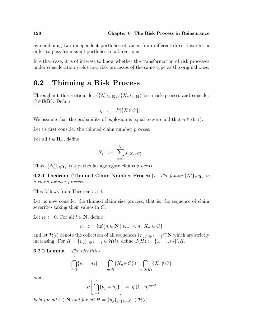
128 Chapter 6 The Risk Process in Reinsurance
by combining two independent portfolios obtained from different direct insurers inorder to pass from small portfolios to a larger one.
In either case, it is of interest to know whether the transformation of risk processesunder consideration yields new risk processes of the same type as the original ones.
6.2 Thinning a Risk Process
Throughout this section, let (Ntt∈R+, Xnn∈N) be a risk process and consider
C∈B(R). Define
η := P [X∈C] .
We assume that the probability of explosion is equal to zero and that η ∈ (0, 1).
Let us first consider the thinned claim number process:
For all t ∈ R+, define
N ′t :=
Nt∑n=1
χXn∈C .
Thus, N ′tt∈R+
is a particular aggregate claims process.
6.2.1 Theorem (Thinned Claim Number Process). The family N ′tt∈R+
isa claim number process.
This follows from Theorem 5.1.4.
Let us now consider the thinned claim size process, that is, the sequence of claimseverities taking their values in C.
Let ν0 := 0. For all l ∈ N, define
νl := infn ∈ N | νl−1 < n, Xn ∈ Cand let H(l) denote the collection of all sequences njj∈1,...,l⊆N which are strictlyincreasing. For H = njj∈1,...,l ∈ H(l), define J(H) := 1, . . . , nl\H.
6.2.2 Lemma. The identities
l⋂j=1
νj = nj =⋂n∈H
Xn∈C ∩⋂
n∈J(H)
Xn /∈C
and
P
[l⋂
j=1
νj = nj]
= ηl(1−η)nl−l
hold for all l ∈ N and for all H = njj∈1,...,l ∈ H(l).
6.2 Thinning a Risk Process 129
It is clear that, for each l ∈N, the family ⋂lj=1νj = njH∈H(l) is disjoint. The
following lemma shows that it is, up to a null set, even a partition of Ω:
6.2.3 Corollary. The identity
∑
H∈H(l)
P
[l⋂
j=1
νj = nj]
= 1
holds for all l ∈ N.
Proof. By induction, we have∑
H∈H(l)
ηl(1−η)nl−l = 1
for all l ∈ N. The assertion now follows from Lemma 6.2.2. 2
The basic idea for proving the principal results of this section will be to computethe probabilities of the events of interest from their conditional probabilities withrespect to events from the partition ⋂l
j=1νj = njH∈H(l) with suitable l ∈ N.
By Corollary 6.2.3, each νn is finite. For all n ∈ N, define
X ′n :=
∞∑
k=1
χνn=kXk .
Then we have σ(X ′nn∈N) ⊆ σ(Xnn∈N).
The following lemma provides the technical tool for the proofs of all further resultsof this section:
6.2.4 Lemma. The identity
P
[k⋂
i=1
X ′i∈Bi ∩
l⋂j=1
νj = nj]
=k∏
i=1
P [X∈Bi|X∈C] · ηl(1−η)nl−l
holds for all k, l ∈ N such that k ≤ l, for all B1, . . . , Bk ∈ B(R), and for everysequence njj∈1,...,l ∈ H(l).
Proof. For every sequence H = njj∈1,...,l ∈ H(l), we have
P
[k⋂
i=1
X ′i∈Bi ∩
l⋂j=1
νj = nj]
= P
[k⋂
i=1
Xni∈Bi ∩
l⋂j=1
νj = nj]
130 Chapter 6 The Risk Process in Reinsurance
= P
[k⋂
i=1
Xni∈Bi ∩
l⋂j=1
Xnj∈C ∩
⋂
n∈J(H)
Xn /∈C]
= P
[k⋂
i=1
Xni∈Bi∩C ∩
l⋂
j=k+1
Xnj∈C ∩
⋂
n∈J(H)
Xn /∈C]
=k∏
i=1
P [X∈Bi∩C] ·l∏
j=k+1
P [X∈C] ·∏
n∈J(H)
P [X /∈C]
=k∏
i=1
P [X∈Bi|X∈C] ·l∏
j=1
P [X∈C] ·∏
n∈J(H)
P [X /∈C]
=k∏
i=1
P [X∈Bi|X∈C] · ηl(1−η)nl−l ,
as was to be shown. 2
6.2.5 Theorem (Thinned Claim Size Process). The sequence X ′nn∈N is
i. i. d. and satisfiesP [X ′∈B] = P [X∈B|X∈C]
for all B ∈ B(R).
Proof. Consider k ∈ N and B1, . . . , Bk ∈ B(R). By Lemmas 6.2.4 and 6.2.2, wehave, for every sequence njj∈1,...,k ∈ H(k),
P
[k⋂
i=1
X ′i∈Bi ∩
k⋂j=1
νj = nj]
=k∏
i=1
P [X∈Bi|X∈C] · ηk(1−η)nk−k
=k∏
i=1
P [X∈Bi|X∈C] · P[
k⋂j=1
νj = nj]
.
By Corollary 6.2.3, summation over H(k) yields
P
[k⋂
i=1
X ′i∈Bi
]=
k∏i=1
P [X∈Bi|X∈C] .
The assertion follows. 2
We can now prove the main result of this section:
6.2.6 Theorem (Thinned Risk Process). The pair (N ′tt∈R+
, X ′nn∈N) is a
risk process.
Proof. By Theorems 6.2.1 and 6.2.5, we know that N ′tt∈R+
is a claim numberprocess and that the sequence X ′
nn∈N is i. i. d.
6.2 Thinning a Risk Process 131
To prove that the pair (N ′tt∈R+
, X ′nn∈N) is independent, consider m,n ∈ N,
B1, . . . , Bn ∈ B(R), t0, t1, . . . , tm ∈ R+ such that 0 = t0 < t1 < . . . < tm, andk0, k1, . . . , km ∈ N0 such that 0 = k0 ≤ k1 ≤ . . . ≤ km.Consider also l0, l1, . . . , lm ∈ N0 satisfying 0 = l0 ≤ l1 ≤ . . . ≤ lm as well askj − kj−1 ≤ lj − lj−1 for all j∈1, . . . , m. Define n0 := 0 and l := maxn, km+1,and let H denote the collection of all sequences njj∈1,...,l ∈ H(l) satisfyingnkj
≤ lj < nkj+1 for all j ∈ 1, . . . ,m. By Lemma 6.2.4 and Theorem 6.2.5, wehave
P
[n⋂
i=1
X ′i∈Bi ∩
m⋂j=1
lj∑
h=1
χXh∈C = kj
]
= P
[n⋂
i=1
X ′i∈Bi ∩
m⋂j=1
νkj≤ lj < νkj+1
]
=∑H∈H
P
[n⋂
i=1
X ′i∈Bi ∩
l⋂j=1
νj = nj]
=∑H∈H
(n∏
i=1
P [X∈Bi|X∈C])
ηl(1−η)nl−l
=∑H∈H
P
[n⋂
i=1
X ′i∈Bi
]ηl(1−η)nl−l
= P
[n⋂
i=1
X ′i∈Bi
]·∑H∈H
ηl(1−η)nl−l ,
hence
P
[n⋂
i=1
X ′i ∈ Bi ∩
m⋂j=1
N ′tj
= kj ∩m⋂
j=1
Ntj = lj]
= P
[n⋂
i=1
X ′i ∈ Bi ∩
m⋂j=1
Ntj∑
h=1
χXh∈C = kj
∩
m⋂j=1
Ntj = lj]
= P
[n⋂
i=1
X ′i ∈ Bi ∩
m⋂j=1
lj∑
h=1
χXh∈C = kj
∩
m⋂j=1
Ntj = lj]
= P
[n⋂
i=1
X ′i ∈ Bi ∩
m⋂j=1
lj∑
h=1
χXh∈C = kj
]· P
[m⋂
j=1
Ntj = lj]
= P
[n⋂
i=1
X ′i∈Bi
]·∑H∈H
ηl(1−η)nl−l · P[
m⋂j=1
Ntj = lj]
,
132 Chapter 6 The Risk Process in Reinsurance
and thus
P
[n⋂
i=1
X ′i ∈ Bi ∩
m⋂j=1
N ′tj
= kj ∩m⋂
j=1
Ntj = lj]
= P
[n⋂
i=1
X ′i∈Bi
]· P
[m⋂
j=1
N ′tj
= kj ∩m⋂
j=1
Ntj = lj]
.
Summation yields
P
[n⋂
i=1
X ′i ∈ Bi ∩
m⋂j=1
N ′tj
= kj]
= P
[n⋂
i=1
X ′i∈Bi
]· P
[m⋂
j=1
N ′tj
= kj]
.
Therefore, the pair (N ′tt∈R+
, X ′nn∈N) is independent. 2
6.2.7 Corollary (Thinned Risk Process). Let h : R → R be a measurablefunction. Then the pair (N ′
tt∈R+, h(X ′
n)n∈N) is a risk process.
This is immediate from Theorem 6.2.6.
As an application of Corollary 6.2.7, consider c ∈ (0,∞), let C := (c,∞), and defineh : R → R by letting
h(x) := (x− c)+ .
In excess of loss reinsurance, c is the priority of the direct insurer, and the reinsureris concerned with the risk process (N ′
tt∈R+, (X ′
n−c)+n∈N).
More generally, consider c, d ∈ (0,∞), let C := (c,∞), and define h : R → R byletting
h(x) := (x− c)+∧ d .
In this case, the reinsurer is not willing to pay more than d for a claim exceedingc and covers only the layer (c, c+d ]; he is thus concerned with the risk process(N ′
tt∈R+, (X ′
n−c)+∧ dn∈N).
Problems6.2.A The sequence νll∈N0
is a claim arrival process (in discrete time) satisfying
Pνl= Geo(l, η)
for all l ∈ N. Moreover, the claim interarrival times are i. i. d. Study also theclaim number process induced by the claim arrival process νll∈N0
.
6.2.B For c ∈ (0,∞) and C := (c,∞), compute the distribution of X ′ for some specificchoices of the distribution of X.
6.2.C Discrete Time Model: The risk process (Nll∈N0, Xnn∈N) is a binomial
risk process if the claim number process Nll∈N0is a binomial process.
Study the problem of thinning for a binomial risk process.
6.3 Decomposition of a Poisson Risk Process 133
6.3 Decomposition of a Poisson Risk Process
Throughout this section, let (Ntt∈R+, Xnn∈N) be a risk process and consider
C∈B(R). Define
η := P [X∈C] .
We assume that the probability of explosion is equal to zero and that η ∈ (0, 1).
Let us first consider the thinned claim number processes generated by the claimswith claim size in C or in C, respectively.
For all t ∈ R+, define
N ′t :=
Nt∑n=1
χXn∈C
and
N ′′t :=
Nt∑n=1
χXn∈C .
By Theorem 6.2.1, N ′tt∈R+
and N ′′t t∈R+
are claim number processes.
The following result improves Corollary 5.1.5:
6.3.1 Theorem (Decomposition of a Poisson Process). Assume thatNtt∈R+
is a Poisson process with parameter α. Then the claim number processesN ′
tt∈R+and N ′′
t t∈R+are independent Poisson processes with parameters αη and
α(1−η), respectively.
Proof. Consider m ∈ N, t0, t1, . . . , tm ∈ R+ such that 0 = t0 < t1 < . . . < tm, andk′1, . . . , k
′m ∈ N0 and k′′1 , . . . , k
′′m ∈ N0.
For all j ∈ 1, . . . ,m, define kj := k′j + k′′j and nj :=∑j
i=1 ki. Then we have
P
[m⋂
j=1
N ′tj−N ′
tj−1= k′j∩N ′′
tj−N ′′
tj−1= k′′j
∣∣∣∣∣m⋂
j=1
Ntj−Ntj−1= kj
]
= P
m⋂j=1
Ntj∑
h=Ntj−1+1
χXh∈C = k′j
∩
Ntj∑
h=Ntj−1+1
χXh∈C = k′′j
∣∣∣∣∣∣
m⋂j=1
Ntj = nj
= P
m⋂j=1
nj∑
h=nj−1+1
χXh∈C = k′j
∩
nj∑
h=nj−1+1
χXh∈C = k′′j
∣∣∣∣∣∣
m⋂j=1
Ntj = nj
134 Chapter 6 The Risk Process in Reinsurance
= P
m⋂j=1
nj∑
h=nj−1+1
χXh∈C = k′j
∩
nj∑
h=nj−1+1
χXh∈C = k′′j
=m∏
j=1
(kj
k′j
)ηk′j(1−η)k′′j
as well as
P
[m⋂
j=1
Ntj−Ntj−1= kj
]=
m∏j=1
P [Ntj−Ntj−1= kj]
=m∏
j=1
e−α(tj−tj−1) (α(tj−tj−1))kj
kj!,
and hence
P
[m⋂
j=1
N ′tj−N ′
tj−1= k′j ∩ N ′′
tj−N ′′
tj−1= k′′j
]
= P
[m⋂
j=1
N ′tj−N ′
tj−1= k′j ∩ N ′′
tj−N ′′
tj−1= k′′j
∣∣∣∣∣m⋂
j=1
Ntj−Ntj−1= kj
]
·P[
m⋂j=1
Ntj−Ntj−1= kj
]
=m∏
j=1
(kj
k′j
)ηk′j(1−η)k′′j ·
m∏j=1
e−α(tj−tj−1) (α(tj−tj−1))kj
kj!
=m∏
j=1
e−αη(tj−tj−1) (αη(tj−tj−1))k′j
k′j!·
m∏j=1
e−α(1−η)(tj−tj−1) (α(1−η)(tj−tj−1))k′′j
k′′j !.
This implies that N ′tt∈R+
and N ′′t t∈R+
are Poisson processes with parametersαη and α(1−η), respectively, and that N ′
tt∈R+and N ′′
t t∈R+are independent. 2
Let us now consider the thinned claim size processes.
Let ν ′0 := 0 and ν ′′0 := 0. For all l ∈ N, define
ν ′l := infn ∈ N | ν ′l−1 < n, Xn ∈ Cand
ν ′′l := infn ∈ N | ν ′′l−1 < n, Xn ∈ C .
For m,n ∈ N0 such that m + n ∈ N, let D′(m,n) denote the collection of all pairsof strictly increasing sequences mii∈1,...,k ⊆ N and njj∈1,...,l ⊆ N satisfying
6.3 Decomposition of a Poisson Risk Process 135
k = m and l ≥ n as well as nl < mk = k + l (such that one of these sequences maybe empty and the union of these sequences is 1, . . . , k + l); similarly, let D′′(m, n)denote the collection of all pairs of strictly increasing sequences mii∈1,...,k ⊆ Nand njj∈1,...,l ⊆ N satisfying l = n and k ≥ m as well as mk < nl = k + l, anddefine
D(m, n) := D′(m,n) +D′′(m,n) .
The collections D(m,n) correspond to the collectionsH(l) considered in the previoussection on thinning.
6.3.2 Lemma. The identitiesk⋂
i=1
ν ′i = mi ∩l⋂
j=1
ν ′′j = nj =k⋂
i=1
Xmi∈ C ∩
l⋂j=1
Xnj∈ C
and
P
[k⋂
i=1
ν ′i = mi ∩l⋂
j=1
ν ′′j = nj]
= ηk(1−η)l
hold for all m,n ∈ N0 such that m+n ∈ N and for all (mii∈1,...,k, njj∈1,...,l) ∈D(m, n).
It is clear that, for every choice of m,n ∈ N0 such that m + n ∈ N, the family⋂k
i=1ν ′i = mi ∩⋂l
j=1ν ′′j = njD∈D(m,n) is disjoint; the following lemma showsthat it is, up to a null set, even a partition of Ω:
6.3.3 Corollary. The identity
∑
D∈D(m,n)
P
[k⋂
i=1
ν ′i = mi ∩l⋂
j=1
ν ′′j = nj]
= 1
holds for all m,n ∈ N0 such that m + n ∈ N.
Proof. For m,n ∈ N0 such that m + n = 1, the identity
∑
D∈D(m,n)
P
[k⋂
i=1
ν ′i = mi ∩l⋂
j=1
ν ′′j = nj]
= 1
follows from Corollary 6.2.3.For m,n∈N, we split D(m,n) into two parts: Let D1(m,n) denote the collection ofall pairs (mii∈1,...,k, njj∈1,...,l) ∈ D(m,n) satisfying m1 = 1, and let D2(m, n)denote the collection of all pairs (mii∈1,...,k, njj∈1,...,l) ∈ D(m,n) satisfyingn1 = 1. Then we have
D(m,n) = D1(m,n) +D2(m, n) .
Furthermore, there are obvious bijections between D1(m,n) and D(m−1, n) andbetween D2(m,n) and D(m,n−1).Using Lemma 6.3.2, the assertion now follows by induction over m + n ∈ N. 2
136 Chapter 6 The Risk Process in Reinsurance
By Corollary 6.2.3, each ν ′n and each ν ′′n is finite. For all n ∈ N, define
X ′n :=
∞∑
k=1
χν′n=kXk
and
X ′′n :=
∞∑
k=1
χν′′n=kXk .
Then we have σ(X ′nn∈N) ∪ σ(X ′′
nn∈N) ⊆ σ(Xnn∈N).
6.3.4 Lemma. The identity
P
[n⋂
h=1
X ′h∈B′
h ∩n⋂
h=1
X ′′h ∈B′′
h ∩k⋂
i=1
ν ′i = mi ∩l⋂
j=1
ν ′′j = nj]
=n∏
h=1
P [X ′h∈B′
h] ·n∏
h=1
P [X ′′h ∈B′′
h] · P[
k⋂i=1
ν ′i = mi ∩l⋂
j=1
ν ′′j = nj]
holds for all n∈N, for all B′1, . . . , B
′n ∈ B(R) and B′′
1 , . . . , B′′n ∈ B(R), and for every
pair (mii∈1,...,k, njj∈1,...,l) ∈ D(n, n).
Proof. By Lemma 6.3.2 and Theorem 6.2.5, we have
P
[n⋂
h=1
X ′h∈B′
h ∩n⋂
h=1
X ′′h ∈B′′
h ∩k⋂
i=1
ν ′i = mi ∩l⋂
j=1
ν ′′j = nj]
= P
[n⋂
h=1
Xmi∈B′
h ∩n⋂
h=1
Xnj∈B′′
h ∩k⋂
i=1
ν ′i = mi ∩l⋂
j=1
ν ′′j = nj]
= P
[n⋂
h=1
Xmi∈B′
h ∩n⋂
h=1
Xnj∈B′′
h ∩k⋂
i=1
Xmi∈C ∩
l⋂j=1
Xnj∈C
]
= P
[n⋂
h=1
Xmi∈B′
h∩C ∩n⋂
h=1
Xnj∈B′′
h∩C ∩k⋂
i=n+1
Xmi∈C ∩
l⋂j=n+1
Xnj∈C
]
=n∏
h=1
P [X∈B′h∩C] ·
n∏
h=1
P [X∈B′′h∩C]
·k∏
i=n+1
P [X∈C] ·l∏
j=n+1
P [X∈C]
=n∏
h=1
P [X∈B′h|X∈C] ·
n∏
h=1
P [X∈B′′h|X∈C]
·k∏
i=1
P [X∈C] ·l∏
j=1
P [X∈C]
6.3 Decomposition of a Poisson Risk Process 137
=n∏
h=1
P [X ′h∈B′
h] ·n∏
h=1
P [X ′′h ∈B′′
h] · ηk(1−η)l
=n∏
h=1
P [X ′h∈B′
h] ·n∏
h=1
P [X ′′h ∈B′′
h] · P[
k⋂i=1
ν ′i = mi ∩l⋂
j=1
ν ′′j = nj]
,
as was to be shown. 2
6.3.5 Theorem (Decomposition of a Claim Size Process). The claim sizeprocesses X ′
nn∈N and X ′′nn∈N are independent.
Proof. Consider n ∈ N, B′1, . . . , B
′n ∈ B(R), and B′′
1 , . . . , B′′n ∈ B(R). By Lemma
6.3.4, we have, for every pair (mii∈1,...,k, njj∈1,...,l) ∈ D(n, n),
P
[n⋂
h=1
X ′h∈B′
h ∩n⋂
h=1
X ′′h ∈B′′
h ∩k⋂
i=1
ν ′i = mi ∩l⋂
j=1
ν ′′j = nj]
=n∏
h=1
P [X ′h∈B′
h] ·n∏
h=1
P [X ′′h ∈B′′
h] · P[
k⋂i=1
ν ′i = mi ∩l⋂
j=1
ν ′′j = nj]
.
By Corollary 6.3.3, summation over D(n, n) yields
P
[n⋂
h=1
X ′h∈B′
h ∩n⋂
h=1
X ′′h ∈B′′
h]
=n∏
h=1
P [X ′h∈B′
h] ·n∏
h=1
P [X ′′h ∈B′′
h] .
The assertion follows. 2
The risk process (Ntt∈R+, Xnn∈N) is a Poisson risk process if the claim number
process Ntt∈R+is a Poisson process.
We can now prove the main result of this section:
6.3.6 Theorem (Decomposition of a Poisson Risk Process). Assume that(Ntt∈R+
, Xnn∈N) is a Poisson risk process. Then (N ′tt∈R+
, X ′nn∈N) and
(N ′′t t∈R+
, X ′′nn∈N) are independent Poisson risk processes.
Proof. By Theorems 6.3.1 and 6.3.5, we know that N ′tt∈R+
and N ′′t t∈R+
areindependent Poisson processes and that X ′
nn∈N and X ′′nn∈N are independent
claim size processes.To prove that the σ–algebras σ(N ′
tt∈R+∪N ′′
t t∈R+) and σ(X ′
nn∈N∪X ′′nn∈N)
are independent, consider m,n∈N, B′1, . . . , B
′n ∈B(R) and B′′
1 , . . . , B′′n ∈B(R), as
well as t0, t1, . . . , tm∈R+ such that 0 = t0 < t1 < . . . < tm and k′1, . . . , k′m∈N0 and
k′′1 , . . . , k′′m∈N0 such that k′1 ≤ . . . ≤ k′m and k′′1 ≤ . . . ≤ k′′m. For all j ∈ 1, . . . , m,
define kj = k′j + k′′j .Furthermore, let p := maxn, k′m, k′′m, and let D denote the collection of all pairs(mii∈1,...,k, njj∈1,...,l) ∈ D(p, p) satisfying maxmk′j , nk′′j = kj for all j ∈1, . . . ,m. By Lemma 6.3.4 and Theorem 6.3.5, we have
138 Chapter 6 The Risk Process in Reinsurance
P
[n⋂
h=1
X ′h∈B′
h∩X ′′h ∈B′′
h ∩m⋂
j=1
kj∑
r=1
χXr∈C = k′j
]
=∑D∈D
P
[n⋂
h=1
X ′h∈B′
h∩X ′′h ∈B′′
h ∩m⋂
j=1
maxν ′k′j , ν′′k′′j = kj
]
=∑D∈D
P
[n⋂
h=1
X ′h∈B′
h∩X ′′h ∈B′′
h ∩k⋂
i=1
ν ′i = mi ∩l⋂
j=1
ν ′′j = nj]
=∑D∈D
(n∏
h=1
P [X ′h∈B′
h] ·n∏
h=1
P [X ′′h ∈B′′
h] · ηk(1−η)l
)
=∑D∈D
P
[n⋂
h=1
X ′h∈B′
h∩X ′′h ∈B′′
h]ηk(1−η)l
= P
[n⋂
h=1
X ′h∈B′
h∩X ′′h ∈B′′
h]·∑D∈D
ηk(1−η)l ,
hence
P
[n⋂
h=1
X ′h∈B′
h∩X ′′h ∈B′′
h ∩m⋂
j=1
N ′tj
= k′j∩N ′′tj
= k′′j ]
= P
[n⋂
h=1
X ′h∈B′
h∩X ′′h ∈B′′
h ∩m⋂
j=1
N ′tj
= k′j∩Ntj = kj]
= P
[n⋂
h=1
X ′h∈B′
h∩X ′′h ∈B′′
h ∩m⋂
j=1
Ntj∑r=1
χXr∈C = k′j
∩Ntj = kj
]
= P
[n⋂
h=1
X ′h∈B′
h∩X ′′h ∈B′′
h ∩m⋂
j=1
kj∑
r=1
χXr∈C = k′j
∩Ntj = kj
]
= P
[n⋂
h=1
X ′h∈B′
h∩X ′′h ∈B′′
h ∩m⋂
j=1
kj∑
r=1
χXr∈C = k′j
· P
[m⋂
j=1
Ntj = kj]
= P
[n⋂
h=1
X ′h∈B′
h∩X ′′h ∈B′′
h]·∑D∈D
ηk(1−η)l · P[
m⋂j=1
Ntj = kj]
,
and thus
P
[n⋂
h=1
X ′h∈B′
h∩X ′′h ∈B′′
h ∩m⋂
j=1
N ′tj
= k′j∩N ′′tj
= k′′j ]
= P
[n⋂
h=1
X ′h∈B′
h∩X ′′h ∈B′′
h]· P
[m⋂
j=1
N ′tj
= k′j∩N ′′tj
= k′′j ]
.
6.3 Decomposition of a Poisson Risk Process 139
Therefore, the σ–algebras σ(N ′tt∈R+
∪N ′′t t∈R+
) and σ(X ′nn∈N∪X ′′
nn∈N) areindependent.The assertion follows. 2
Let S ′tt∈R+and S ′′t t∈R+
denote the aggregate claims processes induced by therisk processes (N ′
tt∈R+, X ′
nn∈N) and (N ′′t t∈R+
, X ′′nn∈N), respectively. In the
case where (Ntt∈R+, Xnn∈N) is a Poisson risk process, one should expect that
the sum of the aggregate claims processes S ′tt∈R+and S ′′t t∈R+
agrees with theaggregate claims process Stt∈R+
. The following result asserts that this is indeedtrue:
6.3.7 Theorem. Assume that (Ntt∈R+, Xnn∈N) is a Poisson risk process.
Then the aggregate claims processes S ′tt∈R+and S ′′t t∈R+
are independent, andthe identity
St = S ′t + S ′′t
holds for all t ∈ R+.
Proof. By Theorem 6.3.6, the aggregate claims processes S ′tt∈R+and S ′′t t∈R+
are independent.For all ω ∈ N ′
t = 0 ∩ N ′′t = 0, we clearly have
S ′t(ω) + S ′′t (ω) = St(ω) .
Consider now k′, k′′ ∈ N0 such that k′ + k′′ ∈ N. Note that maxν ′k′ , ν ′′k′′ ≥ k′+k′′,and that
N ′t = k′ ∩ N ′′
t = k′′ = maxν ′k′ , ν ′′k′′ = k′+k′′ ∩ Nt = k′+k′′ .
Thus, for (mii∈1,...,k, njj∈1,...,l) ∈ D(k′, k′′) satisfying maxmk′ , nk′′ > k′+k′′
the set N ′t = k′ ∩ N ′′
t = k′′ ∩⋂ki=1ν ′i = mi ∩
⋂lj=1ν ′′j = nj is empty, and for
(mii∈1,...,k, njj∈1,...,l) ∈ D(k′, k′′) satisfying maxmk′ , nk′′ = k′+k′′ we have,
for all ω ∈ N ′t = k′ ∩ N ′′
t = k′′ ∩⋂ki=1ν ′i = mi ∩
⋂lj=1ν ′′j = nj,
S ′t(ω) + S ′′t (ω) =
N ′t(ω)∑i=1
X ′i(ω) +
N ′′t (ω)∑j=1
X ′′j (ω)
=k′∑
i=1
X ′i(ω) +
k′′∑j=1
X ′′j (ω)
=k′∑
i=1
Xmi(ω) +
k′′∑j=1
Xnj(ω)
=k′+k′′∑
h=1
Xh(ω)
140 Chapter 6 The Risk Process in Reinsurance
=Nt∑
h=1
Xh(ω)
= St(ω) .
This yields
S ′t(ω) + S ′′t (ω) = St(ω)
for all ω ∈ N ′t = k′ ∩ N ′′
t = k′′.We conclude that
S ′t + S ′′t = St ,
as was to be shown. 2
Problems6.3.A Let (Ntt∈R+
, Xnn∈N) be a Poisson risk process satisfying PX = Exp(β),and let C := (c,∞) for some c ∈ (0,∞).Compute the distributions of X ′ and X ′′, compare the expectation, variance andcoefficient of variation of X ′ and of X ′′ with the corresponding quantities of X,and compute these quantities for S′t, S′′t , and St (see Problem 5.2.G).
6.3.B Extend the results of this section to the decomposition of a Poisson risk processinto more than two Poisson risk processes.
6.3.C Let (Ntt∈R+, Xnn∈N) be a Poisson risk process satisfying PX [1, . . . ,m] = 1
for some m ∈ N. For all j ∈ 1, . . . ,m and t ∈ R+, define
N(j)t :=
Nt∑
n=1
χXn=j .
Then the claim number processes N (1)t t∈R+
, . . . , N (m)t t∈R+
are independent,and the identity
St =m∑
j=1
j N(j)t
holds for all t ∈ R+.
6.3.D Extend the results of this section to the case where the claim number process isan inhomogeneous Poisson process.
6.3.E Discrete Time Model: Study the decomposition of a binomial risk process.
6.3.F Discrete Time Model: Let (Nll∈N0, Xnn∈N) be a binomial risk process
satisfying PX = Geo(η), and let C := (m,∞) for some m ∈ N.Compute the distributions of X ′ and X ′′, compare the expectation, variance andcoefficient of variation of X ′ and of X ′′ with the corresponding quantities of X,and compute these quantities for S′l, S′′l , and Sl.
6.4 Superposition of Poisson Risk Processes 141
6.4 Superposition of Poisson Risk Processes
Throughout this section, let (N ′tt∈R+
, X ′nn∈N) and (N ′′
t t∈R+, X ′′
nn∈N) berisk processes, let T ′
nn∈N0and T ′′
nn∈N0denote the claim arrival processes in-
duced by the claim number processes N ′tt∈R+
and N ′′t t∈R+
, and let W ′nn∈N
and W ′′nn∈N denote the claim interarrival processes induced by the claim arrival
processes T ′nn∈N0
and T ′′nn∈N0
, respectively.
We assume that the risk processes (N ′tt∈R+
, X ′nn∈N) and (N ′′
t t∈R+, X ′′
nn∈N)are independent, that their exceptional null sets are empty, and that the claimnumber processes N ′
tt∈R+and N ′′
t t∈R+are Poisson processes with parameters
α′ and α′′, respectively.
For all t ∈ R+, define
Nt := N ′t + N ′′
t .
The process Ntt∈R+is said to be the superposition of the Poisson processes
N ′tt∈R+
and N ′′t t∈R+
.
The following result shows that the class of all Poisson processes is stable undersuperposition:
6.4.1 Theorem (Superposition of Poisson Processes). The process Ntt∈R+
is a Poisson process with parameter α′ + α′′.
Proof. We first show that Ntt∈R+is a claim number process, and we then prove
that it is indeed a Poisson process. To simplify the notation in this proof, let
α := α′ + α′′ .
(1) Define
ΩN :=⋃
n′,n′′∈N0
T ′n′ = T ′′
n′′ .
Since the claim number processes N ′tt∈R+
and N ′′t t∈R+
are independent andsince the distributions of their claim arrival times are absolutely continuous withrespect to Lebesgue measure, we have
P [ΩN ] = 0 .
It is now easy to see that Ntt∈R+is a claim number process with exceptional null
set ΩN .(2) For all t ∈ R+, we have
E[Nt] = E[N ′t ] + E[N ′′
t ]
= α′t + α′′t
= αt .
142 Chapter 6 The Risk Process in Reinsurance
(3) Let F ′tt∈R+
and F ′′t t∈R+
denote the canonical filtrations of N ′tt∈R+
andN ′′
t t∈R+, respectively, and let Ftt∈R+
denote the canonical filtration of Ntt∈R+.
Using independence of the pair (N ′tt∈R+
, N ′′t t∈R+
) and the martingale propertyof the centered claim number processes N ′
t − α′tt∈R+and N ′′
t − α′′tt∈R+, which
is given by Theorem 2.3.4, we see that the identity
∫
A′∩A′′(Nt+h−Nt−αh) dP
=
∫
A′∩A′′
((N ′
t+h+N ′′t+h)− (N ′
t +N ′′t )− (α′+α′′)h
)dP
=
∫
A′∩A′′(N ′
t+h−N ′t−α′h) dP +
∫
A′∩A′′(N ′′
t+h−N ′′t −α′′h) dP
= P [A′′]∫
A′(N ′
t+h−N ′t−α′h) dP + P [A′]
∫
A′′(N ′′
t+h−N ′′t −α′′h) dP
= 0
holds for all t, h ∈ R+ and for all A′ ∈ F ′t and A′′ ∈ F ′′
t . Thus, letting
Et := A′ ∩ A′′ | A′ ∈ F ′t, A′′ ∈ F ′′
t ,
the previous identity yields
∫
A
(Nt+h − α(t+h)) dP =
∫
A
(Nt − αt) dP
for all t, h ∈ R+ and A ∈ Et. Since Et is stable under intersection and satisfiesFt ⊆ σ(Et), we conclude that the identity
∫
A
(Nt+h − α(t+h)) dP =
∫
A
(Nt − αt) dP
holds for all t, h ∈ R+ and A ∈ Ft. Therefore, the centered claim number processNt−αtt∈R+
is a martingale, and it now follows from Theorem 2.3.4 that the claimnumber process Ntt∈R+
is a Poisson process with parameter α. 2
Let Tnn∈N0denote the claim arrival process induced by the claim number pro-
cess Ntt∈R+and let Wnn∈N denote the claim interarrival process induced by
Tnn∈N0.
To avoid the annoying discussion of null sets, we assume henceforth that the excep-tional null set of the claim number process Ntt∈R+
is empty.
The following result shows that each of the distributions PW ′ and PW ′′ has a densitywith respect to PW :
6.4 Superposition of Poisson Risk Processes 143
6.4.2 Lemma. The distributions PW ′ and PW ′′ satisfy
PW ′ =
∫α′
α′ + α′′eα′′w dPW (w)
and
PW ′′ =
∫α′′
α′ + α′′eα′w dPW (w) .
Proof. Since PW ′ = Exp(α′) and PW = Exp(α′+α′′), we have
PW ′ =
∫α′e−α′w χ(0,∞)(w) dλ(w)
=
∫α′
α′ + α′′eα′′w (α′+α′′) e−(α′+α′′)w χ(0,∞)(w) dλ(w)
=
∫α′
α′ + α′′eα′′w dPW (w) ,
which is the first identity. The second identity follows by symmetry. 2
For l ∈ N and k ∈ 0, 1, . . . , l, let C(l, k) denote the collection of all pairs of strictlyincreasing sequences mii∈1,...,k⊆N and njj∈1,...,l−k⊆N with union 1, . . . , l(such that one of these sequences may be empty).
For l ∈ N, define
C(l) =l∑
k=0
C(l, k) .
The collections C(l) correspond to the collections H(l) and D(m,n) considered inthe preceding sections on thinning and decomposition.
For l ∈ N, k ∈ 0, 1, . . . , l, and C = (mii∈1,...,k, njj∈1,...,l−k) ∈ C(l, k), let
AC :=⋂
i∈1,...,kTmi
= T ′i ∩
⋂
j∈1,...,l−kTnj
= T ′′j .
We have the following lemma:
6.4.3 Lemma. The identity
P [AC ] =
(α′
α′ + α′′
)k(α′′
α′ + α′′
)l−k
holds for all l ∈ N and k ∈ 0, 1, . . . , l and for all C ∈ C(l, k).
144 Chapter 6 The Risk Process in Reinsurance
Proof. Consider C = (mii∈1,...,k, njj∈1,...,l−k) ∈ C(l, k). We prove severalauxiliary results from which the assertion will follow by induction over l ∈ N.(1) If l = 1 and mk = l, then
P [T1 = T ′1] =
α′
α′ + α′′.
We have
T1 < T ′1 =
⋃
t∈QT1 ≤ t < T ′
1
=⋃
t∈QNt ≥ 1∩N ′
t = 0
=⋃
t∈QN ′′
t ≥ 1∩N ′t = 0
=⋃
t∈QT ′′
1 ≤ t < T ′1
= T ′′1 < T ′
1as well as, by a similar argument,
T1 > T ′1 = ∅ ,
and thus
T1 = T ′1 = T ′
1 ≤ T ′′1
= T ′1 < T ′′
1 = W ′
1 < W ′′1 .
(In the sequel, arguments of this type will be tacitly used at several occasions.) NowLemma 6.4.2 yields
P [T1 = T ′1] = P [W ′
1 < W ′′1 ]
=
∫
RP [w < W ′′
1 ] dPW ′1(w)
=
∫
Re−α′′w α′
α′ + α′′eα′′w dPW (w)
=α′
α′ + α′′,
as was to be shown.(2) If l = 1 and nl−k = l, then
P [T1 = T ′′1 ] =
α′′
α′ + α′′.
This follows from (1) by symmetry.
6.4 Superposition of Poisson Risk Processes 145
(3) If l ≥ 2 and mk = l, then
P
[ ⋂
i∈1,...,kTmi
= T ′i ∩
⋂
j∈1,...,l−kTnj
= T ′′j
]
=α′
α′ + α′′· P
[ ⋂
i∈1,...,k−1Tmi
= T ′i ∩
⋂
j∈1,...,l−kTnj
= T ′′j
].
This means that elimination of the event Tmk= T ′
k produces the factor α′/(α′+α′′).To prove our claim, we consider separately the cases mk−1 < l−1 and mk−1 = l−1.Let us first consider the case mk−1 < l−1. For all s, t ∈ (0,∞) such that s ≤ t,Lemma 6.4.2 yields∫
(t−s,∞)
∫
(s+v−t,∞)
dPW ′′(w) dPW ′(v) =
∫
(t−s,∞)
e−α′′(s+v−t) dPW ′(v)
=
∫
(t−s,∞)
e−α′′(s+v−t) α′
α′ + α′′eα′′v dPW (v)
=α′
α′ + α′′e−α′′(s−t)
∫
(t−s,∞)
dPW (v)
=α′
α′ + α′′e−α′′(s−t) e−(α′+α′′)(t−s)
=α′
α′ + α′′e−α′(t−s)
=α′
α′ + α′′
∫
(t−s,∞)
dPW ′(v) .
For integration variables v1, . . . , vk−1 ∈ R and w1, . . . , wl−k ∈ R, define
s :=k−1∑
h=1
vh
and
t :=l−k∑
h=1
wh .
With suitable domains of integration where these are not specified, the identityestablished before yields
P
[ ⋂
i∈1,...,kTmi
= T ′i ∩
⋂
j∈1,...,l−kTnj
= T ′′j
]
= P [. . . < T ′k−1 . . . < T ′′
l−k < T ′k < T ′′
l−k+1]= P [. . . < T ′
k−1 . . . < T ′′l−k < T ′
k−1 + W ′k < T ′′
l−k + W ′′l−k+1]
146 Chapter 6 The Risk Process in Reinsurance
= . . .
∫. . .
∫ ∫
(t−s,∞)
∫
(s+v−t,∞)
dPW ′′l−k+1
(w) dPW ′k(v) dPW ′′
l−k(wl−k) . . . dPW ′
k−1(vk−1) . . .
= . . .
∫. . .
∫ (α′
α′ + α′′
∫
(t−s,∞)
dPW ′k(v)
)dPW ′′
l−k(wl−k) . . . dPW ′
k−1(vk−1) . . .
=α′
α′ + α′′·(
. . .
∫. . .
∫ ∫
(t−s,∞)
dPW ′k(v) dPW ′′
l−k(wl−k) . . . dPW ′
k−1(vk−1) . . .
)
=α′
α′ + α′′· P [. . . < T ′
k−1 . . . < T ′′l−k < T ′
k−1 + W ′k]
=α′
α′ + α′′· P [. . . < T ′
k−1 . . . < T ′′l−k < T ′
k]
=α′
α′ + α′′· P
[ ⋂
i∈1,...,k−1Tmi
= T ′i ∩
⋂
j∈1,...,l−kTnj
= T ′′j
].
Let us now consider the case mk−1 = l−1. For all s, t ∈ (0,∞) such that t ≤ s,Lemma 6.4.2 yields
∫
(0,∞)
∫
(s+v−t,∞)
dPW ′′(w) dPW ′(v) =
∫
(0,∞)
e−α′′(s+v−t) dPW ′(v)
=
∫
(0,∞)
e−α′′(s+v−t) α′
α′ + α′′eα′′v dPW (v)
=α′
α′ + α′′e−α′′(s−t)
=α′
α′ + α′′
∫
(s−t,∞)
dPW ′′(w) .
This yields, as before,
P
[ ⋂
i∈1,...,kTmi
= T ′i ∩
⋂
j∈1,...,l−kTnj
= T ′′j
]
= P [. . . < T ′′l−k . . . < T ′
k−1 < T ′k < T ′′
l−k+1]= P [. . . < T ′′
l−k . . . < T ′k−1 < T ′
k−1 + W ′k < T ′′
l−k + W ′′l−k+1]
= . . .
∫. . .
∫ ∫
(0,∞)
∫
(s+v−t,∞)
dPW ′′l−k+1
(w) dPW ′k(v) dPW ′
k−1(vk−1) . . . dPW ′′
l−k(wl−k) . . .
= . . .
∫. . .
∫ (α′
α′ + α′′
∫
(s−t,∞)
dPW ′′l−k+1
(v)
)dPW ′
k−1(vk−1) . . . dPW ′′
l−k(wl−k) . . .
=α′
α′ + α′′·(
. . .
∫. . .
∫ ∫
(s−t,∞)
dPW ′′l−k+1
(v) dPW ′k−1
(vk−1) . . . dPW ′′l−k
(wl−k) . . .
)
6.4 Superposition of Poisson Risk Processes 147
=α′
α′ + α′′· P [. . . < T ′′
l−k . . . < T ′k−1 < T ′′
l−k + W ′′l−k+1]
=α′
α′ + α′′· P [. . . < T ′′
l−k . . . < T ′k−1 < T ′′
l−k+1]
=α′
α′ + α′′· P
[ ⋂
i∈1,...,k−1Tmi
= T ′i ∩
⋂
j∈1,...,l−kTj = T ′′
j ]
.
This proves our claim.(4) If l ≥ 2 and nl−k = l, then
P
[ ⋂
i∈1,...,kTmi
= T ′i ∩
⋂
j∈1,...,l−kTnj
= T ′′j
]
=α′′
α′ + α′′· P
[ ⋂
i∈1,...,kTmi
= T ′i ∩
⋂
j∈1,...,l−k−1Tnj
= T ′′j
].
This means that elimination of Tnl−k= T ′′
l produces the factor α′′/(α′+α′′). Theidentity follows from (3) by symmetry.(5) Using (1), (2), (3), and (4), the assertion now follows by induction over l∈N. 2
It is clear that, for each l ∈ N, the family ACC∈C(l) is disjoint; we shall now showthat it is, up to a null set, even a partition of Ω.
6.4.4 Corollary. The identity
∑
C∈C(l)P [AC ] = 1
holds for all l ∈ N.
Proof. By Lemma 6.4.3, we have
∑
C∈C(l)P [AC ] =
l∑
k=0
∑
C∈C(l,k)
P [AC ]
=l∑
k=0
(l
k
)(α′
α′ + α′′
)k(α′′
α′ + α′′
)l−k
= 1 ,
as was to be shown. 2
148 Chapter 6 The Risk Process in Reinsurance
6.4.5 Corollary. The identities
l∑
k=1
P [Tl = T ′k] =
α′
α′ + α′′
andl∑
k=1
P [Tl = T ′′k ] =
α′′
α′ + α′′
hold for all l ∈ N.
Proof. For l ∈ N and k ∈ 1, . . . , l, let C(l, k, k) denote the collection of all pairs(mii∈1,...,k, njj∈1,...,l−k) ∈ C(l) satisfying mk = l. Then we have
l∑
k=1
P [Tl = T ′k] =
l∑
k=1
∑
C∈C(l,k,k)
P [AC ]
=l∑
k=1
∑
C∈C(l,k,k)
(α′
α′ + α′′
)k(α′′
α′ + α′′
)l−k
=l∑
k=1
(l − 1
k − 1
)(α′
α′ + α′′
)k(α′′
α′ + α′′
)l−k
=α′
α′ + α′′
l−1∑j=0
(l − 1
j
)(α′
α′ + α′′
)j(α′′
α′ + α′′
)(l−1)−j
=α′
α′ + α′′,
which is the first identity. The second identity follows by symmetry. 2
For all n ∈ N, define
Xn :=n∑
k=1
(χTn=T ′
kX
′k + χTn=T ′′
kX
′′k
).
The sequence Xnn∈N is said to be the superposition of the claim size processesX ′
nn∈N and X ′′nn∈N.
6.4.6 Theorem (Superposition of Claim Size Processes). The sequenceXnn∈N is i. i. d. and satisfies
PX =α′
α′ + α′′PX′ +
α′′
α′ + α′′PX′′ .
6.4 Superposition of Poisson Risk Processes 149
Proof. Consider l ∈ N and B1, . . . , Bl ∈ B(R).For C = (mii∈1,...,k, njj∈1,...,l−k) ∈ C(l), Lemma 6.4.3 yields
P [AC ] =
(α′
α′ + α′′
)k(α′′
α′ + α′′
)l−k
,
and hence
P
[l⋂
h=1
Xh∈Bh ∩ AC
]
= P
[ ⋂
i∈1,...,kX ′
mi∈Bmi
∩⋂
j∈1,...,l−kX ′′
nj∈Bnj
∩ AC
]
=∏
i∈1,...,kP [X ′
mi∈Bmi
] ·∏
j∈1,...,l−kP [X ′′
nj∈Bnj
] · P [AC ]
=∏
i∈1,...,kPX′ [Bmi
] ·∏
j∈1,...,l−kPX′′ [Bnj
] ·(
α′
α′ + α′′
)k(α′′
α′ + α′′
)l−k
=∏
i∈1,...,k
α′
α′ + α′′PX′ [Bmi
] ·∏
j∈1,...,l−k
α′′
α′ + α′′PX′′ [Bnj
] .
By Corollary 6.4.4, summation over C(l) yields
P
[l⋂
h=1
Xh∈Bh]
=∑
C∈C(l)P
[l⋂
h=1
Xh∈Bh ∩ AC
]
=∑
C∈C(l)
( ∏
i∈1,...,k
α′
α′ + α′′PX′ [Bmi
] ·∏
j∈1,...,l−k
α′′
α′ + α′′PX′′ [Bnj
]
)
=l∏
h=1
(α′
α′ + α′′PX′ [Bh] +
α′′
α′ + α′′PX′′ [Bh]
),
and the assertion follows. 2
We can now prove the main result of this section:
6.4.7 Theorem (Superposition of Poisson Risk Processes). The pair(Ntt∈R+
, Xnn∈N) is a Poisson risk process.
Proof. Consider l ∈ N, B1, . . . , Bl ∈ B(R), and a disjoint family Dhh∈1,...,l ofintervals in (0,∞) with increasing lower bounds. Define
η :=l−1∏
h=1
(α′+α′′) λ[Dh] · PW [Dl] .
150 Chapter 6 The Risk Process in Reinsurance
If we can show that
P
[l⋂
h=1
Xh∈Bh ∩ Th∈Dh]
= P
[l⋂
h=1
Xh∈Bh]· η ,
then we have
P
[l⋂
h=1
Xh∈Bh ∩ Th∈Dh]
= P
[l⋂
h=1
Xh∈Bh]· P
[l⋂
h=1
Th∈Dh]
.
We proceed in several steps:(1) The identity
P
[l⋂
h=1
Th∈Dh ∩ AC
]= η ·
(α′
α′ + α′′
)k(α′′
α′ + α′′
)l−k
holds for all C = (mii∈1,...,k, njj∈1,...,l−k) ∈ C(l).Assume that l = mk. For integration variables v1, . . . , vk ∈ R and w1, . . . , wl−k ∈ Rand for i ∈ 0, 1, . . . , k and j ∈ 0, 1, . . . , l−k, define
si :=i∑
h=1
vh
and
tj :=
j∑
h=1
wh .
Using translation invariance of the Lebesgue measure, we obtain
∫
Dn1−t0
. . .
∫
Dnl−k−tl−k−1
eα′′tl−kdPW ′′l−k
(wl−k) . . . dPW ′′1(w1) =
l−k∏j=1
α′′ λ[Dnj] ,
also, using the transformation formula, we obtain∫
Dmk−sk−1
e−α′′sk dPW ′k(vk)
=
∫
Dmk−sk−1
e−α′′sk α′e−α′vk χ(0,∞)(vk) dλ(vk)
=α′
α′ + α′′eα′sk−1
∫
Dmk−sk−1
(α′+α′′) e−(α′+α′′)(sk−1+vk) χ(0,∞)(vk) dλ(vk)
=α′
α′ + α′′eα′sk−1
∫
Dmk
(α′+α′′) e−(α′+α′′)sk χ(0,∞)(sk) dλ(sk)
=α′
α′ + α′′eα′sk−1PW [Dmk
]
=α′
α′ + α′′eα′sk−1PW [Dl] ,

6.4 Superposition of Poisson Risk Processes 151
and hence
∫
Dm1−s0
. . .
∫
Dmk−sk−1
e−α′′skdPW ′k(vk) . . . dPW ′
1(v1) =
α′
α′ + α′′PW [Dl]
k−1∏i=1
α′λ[Dmj] .
This yields
P
[l⋂
h=1
Th∈Dh ∩ AC
]
= P
[k⋂
i=1
T ′i ∈Dmi
∩l−k⋂j=1
T ′′j ∈Dnj
∩ T ′k ≤ T ′′
l−k+1]
= P
[k⋂
i=1
T ′i ∈Dmi
∩l−k⋂j=1
T ′′j ∈Dnj
∩ T ′k ≤ T ′′
l−k + W ′′l−k+1
]
=
∫
Dm1−s0
. . .
∫
Dmk−sk−1
∫
Dn1−t0
. . .
∫
Dnl−k−tl−k−1
∫
(sk−tl−k,∞)
dPW ′′l−k+1
(wl−k+1)
dPW ′′l−k
(wl−k) . . . dPW ′′1(w1) dPW ′
k(vk) . . . dPW ′
1(v1)
=
∫
Dm1−s0
. . .
∫
Dmk−sk−1
∫
Dn1−t0
. . .
∫
Dnl−k−tl−k−1
e−α′′(sk−tl−k)
dPW ′′l−k
(wl−k) . . . dPW ′′1(w1) dPW ′
k(vk) . . . dPW ′
1(v1)
=
∫
Dm1−s0
. . .
∫
Dmk−sk−1
e−α′′sk
(∫
Dn1−t0
. . .
∫
Dnl−k−tl−k−1
eα′′tl−k
dPW ′′l−k
(wl−k) . . . dPW ′′1(w1)
)dPW ′
k(vk) . . . dPW ′
1(v1)
=
∫
Dm1−s0
. . .
∫
Dmk−sk−1
e−α′′sk
(l−k∏j=1
α′′ λ[Dnj]
)dPW ′
k(vk) . . . dPW ′
1(v1)
=α′
α′ + α′′PW [Dl]
k−1∏i=1
α′λ[Dmj] ·
l−k∏j=1
α′′ λ[Dnj]
=
(α′
α′ + α′′
)k(α′′
α′ + α′′
)l−k
·l−1∏
h=1
(α′+α′′) λ[Dh] · PW [Dl]
=
(α′
α′ + α′′
)k(α′′
α′ + α′′
)l−k
· η .
By symmetry, the same result obtains in the case l = nl−k.
152 Chapter 6 The Risk Process in Reinsurance
(2) The identity
P
[l⋂
h=1
Xh∈Bh ∩ Th∈Dh ∩ AC
]
=k∏
i=1
α′
α′ + α′′PX′ [Bmi
] ·l−k∏j=1
α′′
α′ + α′′PX′′ [Bnj
] · η
holds for all C = (mii∈1,...,k, njj∈1,...,l−k) ∈ C(l).Because of (1), we have
P
[l⋂
h=1
Xh∈Bh ∩ Th∈Dh ∩ AC
]
= P
[k⋂
i=1
X ′mi∈Bmi
∩ T ′mi∈Dmi
∩l−k⋂j=1
X ′′nj∈Bnj
∩ T ′′nj∈Dnj
∩ AC
]
= P
[k⋂
i=1
X ′mi∈Bmi
∩l−k⋂j=1
X ′′nj∈Bnj
]
· P[
k⋂i=1
T ′mi∈Dmi
∩l−k⋂j=1
T ′′nj∈Dnj
∩ AC
]
=k∏
i=1
PX′ [Bmi]
l−k∏j=1
PX′′ [Bnj] · P
[l⋂
h=1
Th∈Dh ∩ AC
]
=k∏
i=1
PX′ [Bmi]
l−k∏j=1
PX′′ [Bnj] ·
(α′
α′ + α′′
)k(α′′
α′ + α′′
)l−k
η
=k∏
i=1
α′
α′ + α′′PX′ [Bmi
] ·l−k∏j=1
α′′
α′ + α′′PX′′ [Bnj
] · η ,
as was to be shown.(3) We have
P
[l⋂
h=1
Xh∈Bh ∩ Th∈Dh]
= P
[l⋂
h=1
Xh∈Bh]· η .
By Corollary 6.4.4 and because of (2) and Theorem 6.4.6, we have
P
[l⋂
h=1
Xh∈Bh ∩ Th∈Dh]
=∑
C∈C(l)P
[l⋂
h=1
Xh∈Bh ∩ Th∈Dh ∩ AC
]
6.4 Superposition of Poisson Risk Processes 153
=∑
C∈C(l)
(k∏
i=1
α′
α′ + α′′PX′ [Bmi
] ·l−k∏j=1
α′′
α′ + α′′PX′′ [Bnj
] · η)
= η ·∑
C∈C(l)
(k∏
i=1
α′
α′ + α′′PX′ [Bmi
] ·l−k∏j=1
α′′
α′ + α′′PX′′ [Bnj
]
)
= η ·l∏
h=1
(α′
α′ + α′′PX′ [Bh] +
α′′
α′ + α′′PX′′ [Bh]
)
= η ·l∏
h=1
P [Xh∈Bh]
= η · P[
l⋂
h=1
Xh∈Bh]
,
as was to be shown.(4) We have
P
[l⋂
h=1
Xh∈Bh ∩l⋂
h=1
Th∈Dh]
= P
[l⋂
h=1
Xh∈Bh]· P
[l⋂
h=1
Th∈Dh]
.
This follows from (3).(5) The previous identity remains valid if the sequence Dhh∈1,...,l of intervalsis replaced by a sequence of general Borel sets. This implies that Xnn∈N andTnn∈N0
are independent. 2
Let us finally consider the aggregate claims process Stt∈R+induced by the Poisson
risk process (Ntt∈R+, Xnn∈N). If the construction of the claim size process
Xnn∈N was appropriate, then the aggregate claims process Stt∈R+should agree
with the sum of the aggregate claims processes S ′tt∈R+and S ′′t t∈R+
induced bythe original Poisson risk processes (N ′
tt∈R+, X ′
nn∈N) and (N ′′t t∈R+
, X ′′nn∈N),
respectively. The following result asserts that this is indeed true:
6.4.8 Theorem. The identity
St = S ′t + S ′′t
holds for all t∈R+.
Proof. For all ω ∈ Nt = 0, we clearly have
St(ω) = S ′t(ω) + S ′′t (ω) .
Consider now l ∈ N. For C = (mii∈1,...,k, njj∈1,...,l−k) ∈ C(l), we have
Nt = l ∩ AC = Tl ≤ t < Tl+1 ∩ AC
= T ′k ≤ t < T ′
k+1 ∩ T ′′l−k ≤ t < T ′′
l−k+1 ∩ AC
= N ′t = k ∩ N ′′
t = l−k ∩ AC
154 Chapter 6 The Risk Process in Reinsurance
and hence, for all ω ∈ Nt = l ∩ AC ,
St(ω) =
Nt(ω)∑
h=1
Xh(ω)
=l∑
h=1
Xh(ω)
=k∑
i=1
Xmi(ω) +
l−k∑j=1
Xnj(ω)
=
N ′t(ω)∑i=1
X ′i(ω) +
N ′′t (ω)∑j=1
X ′′j (ω)
= S ′t(ω) + S ′′t (ω) .
By Corollary 6.4.4, this yields
St(ω) = S ′t(ω) + S ′′t (ω)
for all ω ∈ Nt = l.We conclude that
St = S ′t + S ′′t ,
as was to be shown. 2
Problems6.4.A Extend the results of this section to more than two independent Poisson risk
processes.
6.4.B Study the superposition problem for independent risk processes which are notPoisson risk processes.
6.4.C Discrete Time Model: The sum of two independent binomial processes mayfail to be a claim number process.
6.5 Remarks
For theoretical considerations, excess of loss reinsurance is probably the simplestform of reinsurance. Formally, excess of loss reinsurance with a priority held by thedirect insurer is the same as direct insurance with a deductible to be paid by theinsured.
For further information on reinsurance, see Gerathewohl [1976, 1979] and Dienst[1988]; for a discussion of the impact of deductibles, see Sterk [1979, 1980, 1988].
The superposition problem for renewal processes was studied by Stormer [1969].
Chapter 7
The Reserve Process and theRuin Problem
In the present chapter we introduce the reserve process and study the ruin problem.We first extend the model considered so far and discuss some technical aspects ofthe ruin problem (Section 7.1). We next prove Kolmogorov’s inequality for positivesupermartingales (Section 7.2) and then apply this inequality to obtain Lundberg’sinequality for the probability of ruin in the case where the excess premium processhas a superadjustment coefficient (Section 7.3). We finally give some sufficientconditions for the existence of a superadjustment coefficient (Section 7.4).
7.1 The Model
Throughout this chapter, let Ntt∈R+be a claim number process, let Tnn∈N0
bethe claim arrival process induced by the claim number process, and let Wnn∈N bethe claim interarrival process induced by the claim arrival process. We assume thatthe exceptional null set is empty and that the probability of explosion is equal tozero.
Furthermore, let Xnn∈N be a claim size process, let Stt∈R+be the aggregate
claims process induced by the claim number process and the claim size process, andlet κ ∈ (0,∞). For u ∈ (0,∞) and all t ∈ R+, define
Rut := u + κt− St .
Of course, we have Ru0 = u.
Interpretation:– κ is the premium intensity so that κt is the premium income up to time t.– u is the initial reserve.– Ru
t is the reserve at time t when the initial reserve is u.Accordingly, the family Ru
t t∈R+is said to be the reserve process induced by the

156 Chapter 7 The Reserve Process and the Ruin Problem
claim number process, the claim size process, the premium intensity, and the initialreserve.
u »»»»»»»»»»»»»»»»»»»»»»»»»»»»» u + κt
0 -
s
6
0 T1(ω) T2(ω) T3(ω) T4(ω) T5(ω)
t••
•
•
•• St(ω)
Claim Arrival Process and Aggregate Claims Process
We are interested in the ruin problem for the reserve process. This is the problem ofcalculating or estimating the probability of the event that the reserve process fallsbeyond zero at some time.
0 -
u
r
6
T1(ω) T2(ω) T3(ω) T4(ω) T5(ω)
t
»»»»»»»»»»»»»»»»»»»»»»»»»»»»» u + κt
••
•
•
•• Rut (ω)
Claim Arrival Process and Reserve Process
7.1 The Model 157
In order to give a precise formulation of the ruin problem, we need the followingmeasure–theoretic consideration:
Let Ztt∈R+be family of measurable functions Ω → [−∞,∞]. A measurable
function Z : Ω → [−∞,∞] is said to be an essential infimum of Ztt∈R+if it has
the following properties:– P [Z ≤ Zt] = 1 holds for all t ∈ R+, and– every measurable function Y : Ω → [−∞,∞] such that P [Y ≤ Zt] = 1 holds
for all t ∈ R+ satisfies P [Y ≤ Z] = 1.The definition implies that any two essential infima of Ztt∈R+
are identical withprobability one. The almost surely unique essential infimum of the family Ztt∈R+
is denoted by inft∈R+Zt.
7.1.1 Lemma. Every family Ztt∈R+of measurable functions Ω → [−∞,∞]
possesses an essential infimum.
Proof. Without loss of generality, we may assume that Zt(ω) ∈ [−1, 1] holds forall t ∈ R+ and ω ∈ Ω.Let J denote the collection of all countable subsets of R+. For J ∈ J , consider themeasurable function ZJ satisfying
ZJ(ω) = inft∈J Zt(ω) .
Define
c := infJ∈J E[ZJ ] ,
choose a sequence Jnn∈N satisfying
c = infn∈N E[ZJn ] ,
and define J∞ :=⋃
n∈N Jn. Then we have J∞ ∈ J . Since c ≤ E[ZJ∞ ] ≤ E[ZJn ]holds for all n ∈ N, we obtain
c = E[ZJ∞ ] .
For each t ∈ R+, we have ZJ∞∪t = ZJ∞ ∧ Zt, hence
c ≤ E[ZJ∞∪t]
= E[ZJ∞ ∧ Zt]
≤ E[ZJ∞ ]
= c ,
whence
P [ZJ∞∧Zt = ZJ∞] = 1 ,
and thus
P [ZJ∞ ≤ Zt] = 1 .
The assertion follows. 2
158 Chapter 7 The Reserve Process and the Ruin Problem
Let us now return to the reserve process Rut t∈R+
. By Lemma 7.1.1, the reserveprocess has an essential infimum which is denoted by
inft∈R+Ru
t .
In particular, we have inft∈R+Ru
t < 0 ∈ F . The event inft∈R+Ru
t < 0 is calledruin of the reserve process and its probability is denoted by
Ψ(u) := P [inft∈R+Ru
t < 0]in order to emphasize the dependence of the probability of ruin on the initial reserve.
In practice, an upper bound Ψ∗ for the probability of ruin is given in advance andthe insurer is interested to choose the initial reserve u such that
Ψ(u) ≤ Ψ∗ .
In principle, one would like to choose u such that
Ψ(u) = Ψ∗ ,
but the problem of computing the probability of ruin is even harder than the problemof computing the accumulated claims distribution. It is therefore desirable to havean upper bound Ψ′(u) for the probability of ruin when the initial reserve is u, andto choose u such that
Ψ′(u) = Ψ∗ .
Since
Ψ(u) ≤ Ψ′(u) ,
the insurer is on the safe side but possibly binds too much capital.
It is intuitively clear that the time when the reserve process first falls beyond zero forthe first time must be a claim arrival time. To make this point precise, we introducea discretization of the reserve process: For n ∈ N, define
Gn := κWn −Xn ,
and for n ∈ N0 define
Uun := u +
n∑
k=1
Gk .
Of course, we have Uu0 = u.
The sequence Gnn∈N is said to be the excess premium process , and the sequenceUu
nn∈N0is said to be the modified reserve process.
7.1 The Model 159
The following result shows that the probability of ruin is determined by the modifiedreserve process:
7.1.2 Lemma. The probability of ruin satisfies
Ψ(u) = P [infn∈N0Uu
n < 0] .
Proof. Define A := supN0Tn < ∞. For each ω ∈ Ω\A, we have
inft∈R+Ru
t (ω) = inft∈R+
(u + κt−
Nt(ω)∑
k=1
Xk(ω)
)
= infn∈N0inft∈[Tn(ω),Tn+1(ω))
(u + κt−
Nt(ω)∑
k=1
Xk(ω)
)
= infn∈N0inft∈[Tn(ω),Tn+1(ω))
(u + κt−
n∑
k=1
Xk(ω)
)
= infn∈N0
(u + κTn(ω)−
n∑
k=1
Xk(ω)
)
= infn∈N0
(u + κ
n∑
k=1
Wk(ω)−n∑
k=1
Xk(ω)
)
= infn∈N0
(u +
n∑
k=1
(κWk(ω)−Xk(ω))
)
= infn∈N0
(u +
n∑
k=1
Gk(ω)
)
= infn∈N0Uu
n (ω) .
Since the probability of explosion is assumed to be zero, we have P [A] = 0, hence
inft∈R+Ru
t = infn∈N0Uu
n ,
and thus
Ψ(u) = P [inft∈R+Ru
t < 0]= P [infn∈N0
Uun < 0] ,
as was to be shown. 2
160 Chapter 7 The Reserve Process and the Ruin Problem
In the case where the excess premiums are i. i. d. with finite expectation, the previouslemma yields a first result on the probability of ruin which sheds some light on thedifferent roles of the initial reserve and the premium intensity:
7.1.3 Theorem. Assume that the sequence Gnn∈N is i. i. d. with nondegeneratedistribution and finite expectation. If E[G] ≤ 0, then, for every initial reserve, theprobability of ruin is equal to one.
Proof. By the Chung–Fuchs Theorem, we have
1 = P
[lim infn∈N
n∑
k=1
Gk = −∞]
≤ P
[lim infn∈N
n∑
k=1
Gk < −u
]
≤ P
[infn∈N
n∑
k=1
Gk < −u
]
= P [infn∈N Uun < 0] ,
and thus
P [infn∈N Uun < 0] = 1 .
The assertion now follows from Lemma 7.1.2. 2
7.1.4 Corollary. Assume that the sequences Wnn∈N and Xnn∈N are inde-pendent and that each of them is i. i. d. with nondegenerate distribution and finiteexpectation. If κ ≤ E[X]/E[W ], then, for every initial reserve, the probability ofruin is equal to one.
It is interesting to note that Theorem 7.1.3 and Corollary 7.1.4 do not involve anyassumption on the initial reserve.
In the situation of Corollary 7.1.4 we see that, in order to prevent the probability ofruin from being equal to one, the premium intensity must be large enough to ensurethat the expected premium income per claim, κE[W ], is strictly greater than theexpected claim size E[X]. The expected claim size is called the net premium, andthe expected excess premium,
E[G] = κE[W ]− E[X] ,
is said to be the safety loading of the (modified) reserve process. For later reference,we note that the safety loading is strictly positive if and only if the premium intensitysafisfies
κ >E[X]
E[W ].
We shall return to the situation of Corollary 7.1.4 in Section 7.4 below.
7.2 Kolmogorov’s Inequality for Positive Supermartingales 161
7.2 Kolmogorov’s Inequality for PositiveSupermartingales
Our aim is to establish an upper bound for the probability of ruin under a suitableassumption on the excess premium process. The proof of this inequality will bebased on Kolmogorov’s inequality for positive supermartingales which is the subjectof the present section.
Consider a sequence Znn∈N0of random variables having finite expectations and
let Fnn∈N0be the canonical filtration for Znn∈N0
.
A map τ : Ω → N0 ∪∞ is a stopping time for Fnn∈N0if τ =n ∈ Fn holds for
all n ∈ N0, and it is bounded if supω∈Ω τ(ω) < ∞. Let T denote the collection of allbounded stopping times for Fnn∈N0
, and note that N0 ⊆ T.
For τ ∈ T, define
Zτ :=∞∑
n=0
χτ=nZn .
Then Zτ is a random variable satisfying
|Zτ | =∞∑
n=0
χτ=n|Zn|
as well as
E[Zτ ] =∞∑
n=0
∫
τ=nZn dP .
Note that the sums occurring in the definition of Zτ and in the formulas for |Zτ |and E[Zτ ] actually extend only over a finite number of terms.
7.2.1 Lemma (Maximal Inequality). The inequality
P [supn∈N0|Zn| > ε] ≤ 1
εsupτ∈T E|Zτ |
holds for all ε ∈ (0,∞).
Proof. Define
An := |Zn| > ε ∩n−1⋂
k=1
|Zk| ≤ ε .
162 Chapter 7 The Reserve Process and the Ruin Problem
Then we have supN0|Zn| > ε =
∑∞n=0 An and hence
P [supn∈N0|Zn| > ε] =
∞∑n=0
P [An] .
Consider r ∈ N0, and define a random variable τr by letting
τr(ω) :=
n if ω ∈ An and n∈0, 1, . . . , rr if ω ∈ Ω \∑r
n=0 An .
Then we have τr ∈ T, and hence
r∑n=0
P [An] ≤r∑
n=0
1
ε
∫
An
|Zn| dP
=1
ε
r∑n=0
∫
An
|Zτr | dP
≤ 1
ε
∫
Ω
|Zτr | dP
≤ 1
εsupτ∈T E|Zτ | .
Therefore, we have
P [supn∈N0|Zn| > ε] =
∞∑n=0
P [An]
≤ 1
εsupτ∈T E|Zτ | ,
as was to be shown. 2
7.2.2 Lemma. The following are equivalent :
(a) Znn∈N0is a supermartingale.
(b) The inequality E[Zσ] ≥ E[Zτ ] holds for all σ, τ ∈ T such that σ ≤ τ.
Proof. Assume first that (a) holds and consider σ, τ ∈ T such that σ ≤ τ . For allk, n ∈ N0 such that n ≥ k, we have σ = k∩τ ≥ n+1 = σ = k\τ ≤ n ∈ Fn,and thus
∫
σ=k∩τ≥nZn dP =
∫
σ=k∩τ=nZn dP +
∫
σ=k∩τ≥n+1Zn dP
≥∫
σ=k∩τ=nZn dP +
∫
σ=k∩τ≥n+1Zn+1 dP .
7.2 Kolmogorov’s Inequality for Positive Supermartingales 163
Induction yields
∫
σ=kZk dP =
∫
σ=k∩τ≥kZk dP
≥∞∑
n=k
∫
σ=k∩τ=nZn dP ,
and this gives
∫
Ω
Zσ dP =∞∑
k=0
∫
σ=kZk dP
≥∞∑
k=0
∞∑
n=k
∫
σ=k∩τ=nZn dP
=∞∑
n=0
n∑
k=0
∫
σ=k∩τ=nZn dP
=∞∑
n=0
∫
τ=nZn dP
=
∫
Ω
Zτ dP .
Therefore, (a) implies (b).Assume now that (b) holds. Consider n ∈ N0 and A ∈ Fn, and define a randomvariable τ by letting
τ(ω) :=
n + 1 if ω ∈ An if ω ∈ Ω\A .
Then we have n ≤ τ ∈ T, hence
∫
A
Zn dP +
∫
Ω\AZn dP =
∫
Ω
Zn dP
≥∫
Ω
Zτ dP
=
∫
A
Zn+1 dP +
∫
Ω\AZn dP ,
and thus∫
A
Zn dP ≥∫
A
Zn+1 dP .
Therefore, (b) implies (a). 2
164 Chapter 7 The Reserve Process and the Ruin Problem
7.2.3 Lemma. The following are equivalent :(a) Znn∈N0
is a martingale.(b) The identity E[Zσ] = E[Zτ ] holds for all σ, τ ∈ T.
The proof of Lemma 7.2.3 is similar to that of Lemma 7.2.2.
The sequence Znn∈N0is positive if each Zn is positive.
7.2.4 Corollary (Kolmogorov’s Inequality). If Znn∈N0is a positive super-
martingale, then the inequality
P [supn∈N0Zn > ε] ≤ 1
εE[Z0]
holds for all ε ∈ (0,∞).
This is immediate from Lemmas 7.2.1 and 7.2.2.
7.3 Lundberg’s Inequality
Throughout this section, we assume that the sequence of excess premiums Gnn∈Nis independent.
A constant % ∈ (0,∞) is a superadjustment coefficient for the excess premium processGnn∈N if it satisfies
E[e−%Gn
] ≤ 1
for all n ∈ N, and it is an adjustment coefficient for the excess premium process ifit satisfies
E[e−%Gn
]= 1
for all n ∈ N. The excess premium process need not possess a superadjustmentcoefficient; if the distribution of some excess premium is nondegenerate, then theexcess premium process has at most one adjustment coefficient.
Let Fnn∈N0denote the canonical filtration for Uu
nn∈N0.
7.3.1 Lemma. For % ∈ (0,∞), the identity
∫
A
e−%Uun+1 dP =
∫
A
e−%Uun dP ·
∫
Ω
e−%Gn+1 dP
holds for all n ∈ N0 and A ∈ Fn.
7.3 Lundberg’s Inequality 165
Proof. For all n ∈ N0, we have
Fn = σ(Uu
k k∈0,1,...,n)
= σ(Gkk∈1,...,n
).
Since the sequence Gnn∈N is independent, this yields∫
A
e−%Uun+1 dP =
∫
Ω
χAe−%(Uun+Gn+1) dP
=
∫
Ω
χAe−%Uun e−%Gn+1 dP
=
∫
Ω
χAe−%Uun dP ·
∫
Ω
e−%Gn+1 dP
=
∫
A
e−%Uun dP ·
∫
Ω
e−%Gn+1 dP ,
for all n ∈ N0 and A ∈ Fn. The assertion follows. 2
As an immediate consequence of Lemma 7.3.1, we obtain the following characteri-zations of superadjustment coefficients and adjustment coefficients:
7.3.2 Corollary. For % ∈ (0,∞), the following are equivalent :(a) % is a superadjustment coefficient for the excess premium process.(b) For every u ∈ (0,∞), the sequence e−%Uu
nn∈N0is a supermartingale.
7.3.3 Corollary. For % ∈ (0,∞), the following are equivalent :(a) % is an adjustment coefficient for the excess premium process.(b) For every u ∈ (0,∞), the sequence e−%Uu
nn∈N0is a martingale.
The main result of this section is the following:
7.3.4 Theorem (Lundberg’s Inequality). If % ∈ (0,∞) is a superadjustmentcoefficient for the excess premium process, then the identity
P [infn∈N0Uu
n < 0] ≤ e−%u
holds for all u ∈ (0,∞).
Proof. By Corollaries 7.3.2 and 7.2.4, we have
P [infn∈N0Uu
n < 0] = P[
supn∈N0e−%Uu
n > 1]
≤ E[e−%Uu
0]
= E[e−%u
]
= e−%u ,
as was to be shown. 2
The upper bound for the probability of ruin provided by Lundberg’s inequalitydepends explicitly on the initial reserve u. Implicitly, it also depends, via the super-adjustment coefficient %, on the premium intensity κ.
166 Chapter 7 The Reserve Process and the Ruin Problem
Problem7.3.A Assume that the sequence Xnn∈N is independent. If there exists some %∈(0,∞)
satisfying E[e%Xn ] ≤ 1 for all n ∈ N, then the inequality
P [supt∈R+St > c] ≤ e−%c
holds for all c ∈ (0,∞).Hint: Extend Lemma 7.1.2 and Lundberg’s inequality to the case κ = 0.
7.4 On the Existence of a SuperadjustmentCoefficient
In the present section, we study the existence of a (super)adjustment coefficient.
We first consider the case where the excess premiums are i. i. d. According to thefollowing result, we have to assume that the safety loading is strictly positive:
7.4.1 Theorem. Assume that the sequence Gnn∈N is i. i. d. with nondegeneratedistribution and finite expectation. If the excess premium process has a superadjust-ment coefficient, then E[G] > 0.
Proof. The assertion follows from Theorems 7.3.4 and 7.1.3. 2
7.4.2 Corollary. Assume that the sequences Wnn∈N and Xnn∈N are inde-pendent and that each of them is i. i. d. with nondegenerate distribution and finiteexpectation. If the excess premium process has a superadjustment coefficient, thenκ > E[X]/E[W ].
The previous result has a partial converse:
7.4.3 Theorem. Assume that(i) Wnn∈N and Xnn∈N are independent,(ii) Wnn∈N is i. i. d. and satisfies supz ∈ R+ |E[ezW ] < ∞ ∈ (0,∞], and(iii) Xnn∈N is i. i. d. and satisfies supz ∈ R+ |E[ezX ] < ∞ ∈ (0,∞) as well as
PX [R+] = 1.If κ > E[X]/E[W ], then the excess premium process has an adjustment coefficient.
Proof. By assumption, the sequence Gnn∈N is i. i. d. For all z ∈ R, we have
E[e−zG
]= E
[e−zκW
]E
[ezX
],
and hence
MG(−z) = MW (−κz) MX(z) .
7.4 On the Existence of a Superadjustment Coefficient 167
By assumption, there exists some z′ ∈ (0,∞) such that the moment generatingfunctions of W and of X are both finite on the interval (−∞, z′). Differentiationgives
−M ′G(z) = −κM ′
W (−κz) MX(z) + MW (−κz) M ′X(z)
for all z in a neighbourhood of 0, and thus
M ′G(0) = κE[W ]− E[X] .
By assumption, there exists some z∗ ∈ (0,∞) satisfying MX(z∗) = ∞ and henceMG(−z∗) = ∞. Since MG(0) = 1 and M ′
G(0) > 0, it follows that there existssome % ∈ (0, z∗) satisfying E[e−%G] = MG(−%) = 1. But this means that % is anadjustment coefficient for the excess premium process. 2
In Corollary 7.4.2 and Theorem 7.4.3, the claim interarrival times are i. i. d., whichmeans that the claim number process is a renewal process. A particular renewalprocess is the Poisson process:
7.4.4 Corollary. Assume that(i) Ntt∈R+
and Xnn∈N are independent,(ii) Ntt∈R+
is a Poisson process with parameter α, and(iii) Xnn∈N is i. i. d. and satisfies supz ∈ R+ |E[ezX ] < ∞ ∈ (0,∞) as well as
PX [R+] = 1.If κ > αE[X], then the excess premium process has an adjustment coefficient.
Proof. By Lemmas 2.1.3 and 1.1.1, the claim interarrival process Wnn∈N andthe claim size process Xnn∈N are independent.By Theorem 2.3.4, the sequence Wnn∈N is i. i. d. with PW = Exp(α), and thisyields supz ∈ R+ |E[ezW ] < ∞ = α and E[W ] = 1/α.The assertion now follows from Theorem 7.4.3. 2
In order to apply Lundberg’s inequality, results on the existence of an adjustmentcoefficient are, of course, not sufficient; instead, the adjustment coefficient has to bedetermined explicitly. To this end, the distributions of the excess premiums haveto be specified, and this is usually done by specifying the distributions of the claiminterarrival times and those of the claim severities.
7.4.5 Theorem. Assume that(i) Ntt∈R+
and Xnn∈N are independent,(ii) Ntt∈R+
is a Poisson process with parameter α, and(iii) Xnn∈N is i. i. d. and satisfies PX = Exp(β).If κ > α/β, then β−α/κ is an adjustment coefficient for the excess premium process.In particular,
P [infn∈N Uun < 0] ≤ e−(β−α/κ)u .
168 Chapter 7 The Reserve Process and the Ruin Problem
Proof. By Theorem 2.3.4, the sequence Wnn∈N is i. i. d. with PW = Exp(α).Define
% := β − α
κ.
Then we have
E[e−%G
]= E
[e−%κW ] E[e%X
]
= MW (−%κ) MX(%)
=α
α + %κ
β
β − %
= 1 ,
which means that % is an adjustment coefficient for the excess premium process.The inequality for the probability of ruin follows from Theorem 7.3.4. 2
In the previous result, the bound for the probability of ruin decreases when eitherthe initial reserve or the premium intensity increases.
Let us finally turn to a more general situation in which the excess premiums are stillindependent but need not be identically distributed. In this situation, the existenceof an adjustment coefficient cannot be expected, and superadjustment coefficientscome into their own right:
7.4.6 Theorem. Let αnn∈N and βnn∈N be two sequences of real numbers in(0,∞) such that α := supn∈N αn < ∞ and β := infn∈N βn > 0. Assume that(i) Ntt∈R+
and Xnn∈N are independent,(ii) Ntt∈R+
is a regular Markov process with intensities λnn∈N satisfyingλn(t) = αn for all n ∈ N and t ∈ R+, and
(iii) Xnn∈N is independent and satisfies PXn = Exp(βn) for all n ∈ N.If κ > α/β, then β−α/κ is a superadjustment coefficient for the excess premiumprocess. In particular,
P [infn∈N Uun < 0] ≤ e−(β−α/κ)u .
Proof. By Theorem 3.4.2, the sequence Wnn∈N is independent and satisfiesPWn = Exp(αn) for all n ∈ N. Define
% := β − α
κ.
As in the proof of Theorem 7.4.5, we obtain
E[e−%Gn
]= E
[e−%κWn
]E
[e%Xn
]
7.5 Remarks 169
= E[e−%κW ] E[e%X
]
=αn
αn + %κ
βn
βn − %
=αnβn
αnβn + %(βnκ− %κ− αn)
=αnβn
αnβn + %((βn−β)κ + (α−αn))
≤ 1 ,
which means that % is a superadjustment coefficient for the excess premium process.The inequality for the probability of ruin follows from Theorem 7.3.4. 2
The previous result, which includes Theorem 7.4.5 as a special case, is a ratherexceptional example where a superadjustment coefficient does not only exist butcan even be given in explicit form.
Problems7.4.A In Theorem 7.4.3 and Corollary 7.4.4, the condition on MX is fulfilled whenever
PX = Exp(β), PX = Geo(η), or PX = Log(η).
7.4.B Discrete Time Model: Assume that(i) Nll∈N0
and Xnn∈N are independent,(ii) Nll∈N0
is a binomial process with parameter ϑ, and(iii) Xnn∈N is i. i. d. and satisfies supz ∈ R+ |E[ezX ] < ∞ ∈ (0,∞) as well
as PX [R+] = 1.If κ > ϑE[X], then the excess premium process has an adjustment coefficient.
7.5 Remarks
In the discussion of the ruin problem, we have only considered a fixed premiumintensity and a variable initial reserve. We have done so in order not to overburdenthe notation and to clarify the role of (super)adjustment coefficients, which dependon the premium intensity but not on the initial reserve. Of course, the premiumintensitiy may be a decision variable as well which can be determined by a givenupper bound for the probability of ruin, but the role of the initial reserve and therole of the premium intensity are nevertheless quite different since the former islimited only by the financial power of the insurance company while the latter is toa large extent constrained by market conditions.
The (super)martingale approach to the ruin problem is due to Gerber [1973, 1979]and has become a famous method in ruin theory; see also DeVylder [1977], Delbaenand Haezendonck [1985], Rhiel [1986, 1987], Bjork and Grandell [1988], Dassios and
170 Chapter 7 The Reserve Process and the Ruin Problem
Embrechts [1989], Grandell [1991], Møller [1992], Embrechts, Grandell, and Schmidli[1993], Embrechts and Schmidli [1994], Møller [1995], and Schmidli [1995].
The proof of Kolmogorov’s inequality is usually based on the nontrivial fact that asupermartingale Znn∈N0
satisfies E[Z0] ≥ E[Zτ ] for arbitrary stopping times τ ;see Neveu [1972]. The simple proof presented here is well–known in the theory ofasymptotic martingales; see Gut and Schmidt [1983] for a survey and references.
Traditionally, Lundberg’s inequality is proven under the assumption that % is an ad-justment coefficient; the extension to the case of a superadjustment coefficient is dueto Schmidt [1989]. The origin of this extension, which is quite natural with regardto the use of Kolmogorov’s inequality and the relation between (super)adjustmentcoefficients and (super)martingales, is in a paper by Mammitzsch [1986], who alsopointed out that in the case of i. i. d. excess premiums a superadjustment coefficientmay exist when an adjustment does not exist.
For a discussion of the estimation problem for the (super)adjustment coefficient, seeHerkenrath [1986], Deheuvels and Steinebach [1990], Csorgo and Steinebach [1991],Embrechts and Mikosch [1991], and Steinebach [1993].
Although Theorem 7.4.3 provides a rather general condition under which an adjust-ment coefficient exists, there are important claim size distributions which do notsatisfy these conditions; an example is the Pareto distribution, which assigns highprobability to large claims. For a discussion of the ruin problem for such heavy tailedclaim size distributions, see Thorin and Wikstad [1977], Seal [1980], Embrechts andVeraverbeke [1982], Embrechts and Villasenor [1988], Kluppelberg [1989], and Beir-lant and Teugels [1992].
A natural extension of the model considered in this chapter is to assume that thepremium income is not deterministic but stochastic; see Buhlmann [1972], DeVylder[1977], Dassios and Embrechts [1989], Dickson [1991], and Møller [1992].
While the (homogeneous) Poisson process still plays a prominent role in ruin theory,there are two major classes of claim number processes, renewal processes and Coxprocesses, which present quite different extensions of the Poisson process and forwhich the probability of ruin has been studied in detail. Recent work focusses on Coxprocesses, or doubly stochastic Poisson processes, which are particularly interestingsince they present a common generalization of the inhomogeneous Poisson processand the mixed Poisson process; see e. g. Grandell [1991] and the references giventhere.
Let us finally remark that several authors have also studied the probability that thereserve process attains negative values in a bounded time interval; for a discussionof such finite time ruin probabilities, see again Grandell [1991].
Appendix: Special Distributions
In this appendix we recall the definitions and some properties of the probabilitydistributions which are used or mentioned in the text. For comments on applicationsof these and other distributions in risk theory, see Panjer and Willmot [1992].
Auxiliary Notions
The Gamma Function
The map Γ : (0,∞) → (0,∞) given by
Γ(γ) :=
∫ ∞
0
e−x xγ−1 dx
is called the gamma function. It has the following properties:
Γ(1/2) =√
π
Γ(1) = 1
Γ(γ+1) = γ Γ(γ)
In particular, the identity
Γ(n+1) = n!
holds for all n∈N0. Roughly speaking, the values of the gamma function correspondto factorials.
The Beta Function
The map B : (0,∞)×(0,∞) given by
B(α, β) :=
∫ 1
0
xα−1 (1−x)β−1 dx
is called the beta function. The fundamental identity for the beta function is
B(α, β) =Γ(α) Γ(β)
Γ(α+β),
172 Appendix: Special Distributions
showing that the properties of the beta function follow from those of the gammafunction. Roughly speaking, the inverted values of the beta function correspond tobinomial coefficients.
The Generalized Binomial Coefficient
For α ∈ R and m ∈ N0, the generalized binomial coefficient is defined to be(
α
m
):=
m−1∏j=0
α− j
m− j.
For α ∈ (0,∞), the properties of the gamma function yield the identity(
α + m− 1
m
)=
Γ(α + m)
Γ(α) m!
which is particularly useful.
Measures
We denote by ξ : B(R) → R the counting measure concentrated on N0, and wedenote by λ : B(R) → R the Lebesgue measure. These measures are σ–finite, andthe most important probability measures B(R) → [0, 1] are absolutely continuouswiht respect to either ξ or λ.
For n ∈ N, we denote by λn : B(Rn) → R the n–dimensional Lebesgue measure.
Generalities on Distributions
A probability measure Q : B(Rn) → [0, 1] is called a distribution.
A distribution Q is degenerate if there exists some y ∈ Rn satisfying
Q[y] = 1 ,
and it is nondegenerate if it is not degenerate.
In the remainder of this appendix, we consider only distributions B(R) → [0, 1].
For y ∈ R, the Dirac distribution δy is defined to be the (degenerate) distributionQ satisfying
Q[y] = 1 .
Because of the particular role of the Dirac distribution, all parametric classes ofdistributions considered below are defined as to exclude degenerate distributions.
Let Q and R be distributions B(R) → [0, 1].
Generalities on Distributions 173
Expectation and Higher Moments
If
min
∫
(−∞,0]
(−x) dQ(x),
∫
[0,∞)
x dQ(x)
< ∞ ,
then the expectation of Q is said to exist and is defined to be
E[Q] :=
∫
Rx dQ(x) ;
if
max
∫
(−∞,0]
(−x) dQ(x),
∫
[0,∞)
x dQ(x)
< ∞
or, equivalently, ∫
R|x| dQ(x) < ∞ ,
then the expectation of Q exists and is said to be finite. In this case, Q is said tohave finite expectation.
More generally, if, for some n ∈ N,∫
R|x|n dQ(x) < ∞ ,
then Q is said to have a finite moment of order n or to have a finite n–th momentand the n–th moment of Q is defined to be∫
Rxn dQ(x) .
If Q has a finite moment of order n, then it also has a finite moment of order k forall k ∈ 1, . . . , n − 1. The distribution Q is said to have finite moments of anyorder if ∫
R|x|n dQ(x) < ∞
holds for all n ∈ N.
Variance and Coefficient of Variation
If Q has finite expectation, then the variance of Q is defined to be
var [Q] :=
∫
R(x− E[Q])2 dQ(x) .
If Q satisfies Q[R+] = 1 and E[Q] ∈ (0,∞), then the coefficient of variation of Q isdefined to be
v[Q] :=
√var [Q]E[Q]
.
174 Appendix: Special Distributions
Characteristic Function
The characteristic function or Fourier transform of Q is defined to be the mapϕQ : R → C given by
ϕQ(z) :=
∫
Reizx dQ(x) .
Obviously, ϕQ(0) = 1. Moreover, a deep result on Fourier transforms asserts thatthe distribution Q is uniquely determined by its characteristic function ϕQ.
Moment Generating Function
The moment generating function of Q is defined to be the map MQ : R → [0,∞]given by
MQ(z) :=
∫
Rezx dQ(x) .
Again, MQ(0) = 1. Moreover, if the moment generating function of Q is finite in aneighbourhood of zero, then Q has finite moments of any order and the identity
dnMQ
dzn(0) =
∫
Rxn dQ(x)
holds for all n ∈ N.
Probability Generating Function
If Q[N0] = 1, then the probability generating function of Q is defined to be the mapmQ : [−1, 1] → R given by
mQ(z) :=
∫
Rzx dQ(x)
=∞∑
n=0
zn Q[n] .
Since the identity
1
n!
dnmQ
dzn(0) = Q[n]
holds for all n ∈ N0, the distribution Q is uniquely determined by its probabilitygenerating function mQ. The probability generating function has a unique extensionto the closed unit disc in the complex plane.
Discrete Distributions 175
Convolution
If + : R2 → R is defined to be the map given by +(x, y) := x + y, then
Q ∗R := (Q⊗R)+
is a distribution which is called the convolution of Q and R. The convolution satisfies
ϕQ∗R = ϕQ · ϕR ,
and hence Q ∗R = R ∗Q, as well as
MQ∗R = MQ ·MR ;
also, if Q[N0] = 1 = R[N0], then
mQ∗R = mQ ·mR .
If Q and R have finite expectations, then
E[Q ∗R] = E[Q] + E[R] ,
and if Q and R both have a finite second moment, then
var [Q ∗R] = var [Q] + var [R] .
Furthermore, the identity
(Q∗R)[B] =
∫
RQ[B−y] dR(y)
holds for all B ∈ B(R); in particular, Q ∗ δy = δy ∗Q is the translation of Q by y.If Q =
∫f dν and R =
∫g dν for ν∈ξ, λ, then Q ∗R =
∫f∗g dν, where the map
f ∗g : R → R+ is defined by
(f ∗g)(x) :=
∫
Rf(x−y)g(y) dν(y) .
For n ∈ N0, the n–fold convolution of Q is defined to be
Q∗n :=
δ0 if n = 0Q ∗Q∗(n−1) if n ∈ N
If Q =∫
f dν for ν∈ξ,λ, then the density of Q∗n with respect to ν is denoted f ∗n.
Discrete Distributions
A distribution Q : B(R) → [0, 1] is discrete if there exists a countable set S ∈ B(R)satisfying Q[S] = 1. If Q[N0] = 1, then Q is absolutely continuous with respect to ξ.For detailed information on discrete distributions, see Johnson and Kotz [1969] andJohnson, Kotz, and Kemp [1992].
176 Appendix: Special Distributions
The Binomial Distribution
For m ∈ N and ϑ ∈ (0, 1), the binomial distribution B(m,ϑ) is defined to be thedistribution Q satisfying
Q[x] =
(m
x
)ϑx(1−ϑ)m−x
for all x ∈ 0, 1, . . . , m.
Expectation:
E[Q] = mϑ
Variance:
var [Q] = mϑ(1−ϑ)
Characteristic function:
ϕQ(z) = ((1−ϑ) + ϑeiz)m
Moment generating function:
MQ(z) = ((1−ϑ) + ϑez)m
Probability generating function:
mQ(z) = ((1−ϑ) + ϑz)m
Special case: The Bernoulli distribution B(ϑ) := B(1, ϑ).
The Delaporte Distribution
For α, β ∈ (0,∞) and ϑ ∈ (0, 1), the Delaporte distribution Del(α, β, ϑ) is definedto be the distribution
Q := P(α) ∗NB(β, ϑ) .
The Geometric Distribution
For m ∈ N and ϑ ∈ (0, 1), the geometric distribution Geo(m,ϑ) is defined to bethe distribution
Q := δm ∗NB(m,ϑ) .
Special case: The one–parameter geometric distribution Geo(ϑ) := Geo(1, ϑ).
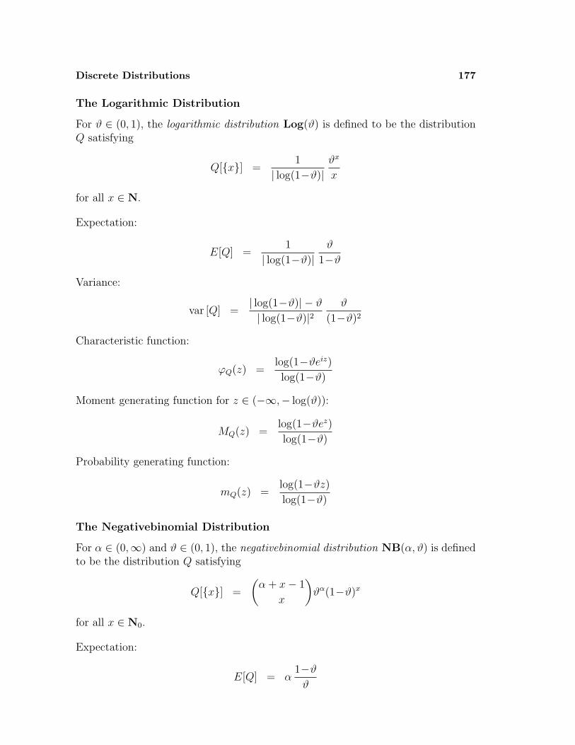
Discrete Distributions 177
The Logarithmic Distribution
For ϑ ∈ (0, 1), the logarithmic distribution Log(ϑ) is defined to be the distributionQ satisfying
Q[x] =1
| log(1−ϑ)|ϑx
x
for all x ∈ N.
Expectation:
E[Q] =1
| log(1−ϑ)|ϑ
1−ϑ
Variance:
var [Q] =| log(1−ϑ)| − ϑ
| log(1−ϑ)|2ϑ
(1−ϑ)2
Characteristic function:
ϕQ(z) =log(1−ϑeiz)
log(1−ϑ)
Moment generating function for z ∈ (−∞,− log(ϑ)):
MQ(z) =log(1−ϑez)
log(1−ϑ)
Probability generating function:
mQ(z) =log(1−ϑz)
log(1−ϑ)
The Negativebinomial Distribution
For α ∈ (0,∞) and ϑ ∈ (0, 1), the negativebinomial distribution NB(α, ϑ) is definedto be the distribution Q satisfying
Q[x] =
(α + x− 1
x
)ϑα(1−ϑ)x
for all x ∈ N0.
Expectation:
E[Q] = α1−ϑ
ϑ
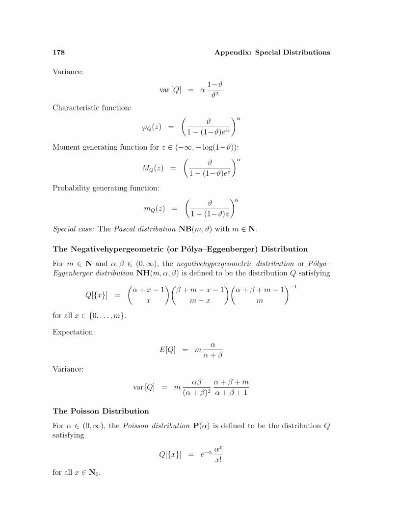
178 Appendix: Special Distributions
Variance:
var [Q] = α1−ϑ
ϑ2
Characteristic function:
ϕQ(z) =
(ϑ
1− (1−ϑ)eiz
)α
Moment generating function for z ∈ (−∞,− log(1−ϑ)):
MQ(z) =
(ϑ
1− (1−ϑ)ez
)α
Probability generating function:
mQ(z) =
(ϑ
1− (1−ϑ)z
)α
Special case: The Pascal distribution NB(m,ϑ) with m ∈ N.
The Negativehypergeometric (or Polya–Eggenberger) Distribution
For m ∈ N and α, β ∈ (0,∞), the negativehypergeometric distribution or Polya–Eggenberger distribution NH(m,α, β) is defined to be the distribution Q satisfying
Q[x] =
(α + x− 1
x
)(β + m− x− 1
m− x
)(α + β + m− 1
m
)−1
for all x ∈ 0, . . . ,m.Expectation:
E[Q] = mα
α + β
Variance:
var [Q] = mαβ
(α + β)2
α + β + m
α + β + 1
The Poisson Distribution
For α ∈ (0,∞), the Poisson distribution P(α) is defined to be the distribution Qsatisfying
Q[x] = e−α αx
x!
for all x ∈ N0.
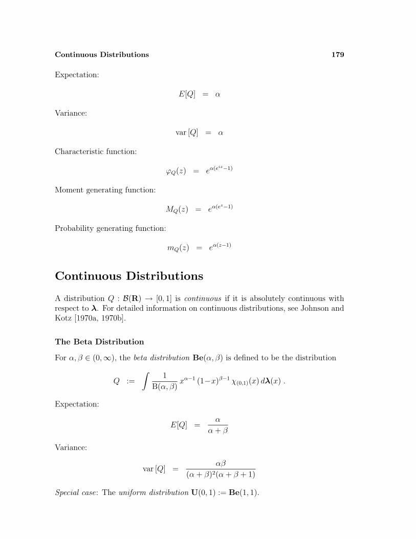
Continuous Distributions 179
Expectation:
E[Q] = α
Variance:
var [Q] = α
Characteristic function:
ϕQ(z) = eα(eiz−1)
Moment generating function:
MQ(z) = eα(ez−1)
Probability generating function:
mQ(z) = eα(z−1)
Continuous Distributions
A distribution Q : B(R) → [0, 1] is continuous if it is absolutely continuous withrespect to λ. For detailed information on continuous distributions, see Johnson andKotz [1970a, 1970b].
The Beta Distribution
For α, β ∈ (0,∞), the beta distribution Be(α, β) is defined to be the distribution
Q :=
∫1
B(α, β)xα−1 (1−x)β−1 χ(0,1)(x) dλ(x) .
Expectation:
E[Q] =α
α + β
Variance:
var [Q] =αβ
(α + β)2(α + β + 1)
Special case: The uniform distribution U(0, 1) := Be(1, 1).
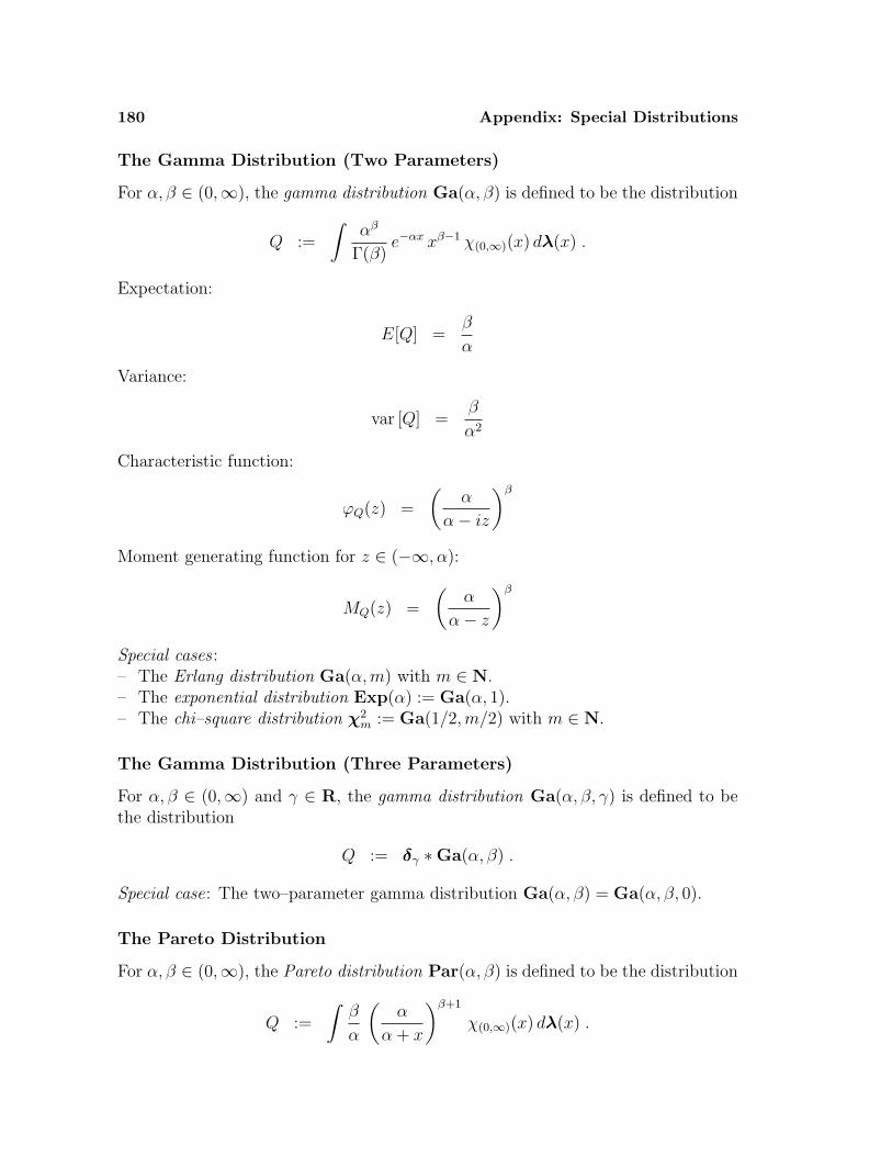
180 Appendix: Special Distributions
The Gamma Distribution (Two Parameters)
For α, β ∈ (0,∞), the gamma distribution Ga(α, β) is defined to be the distribution
Q :=
∫αβ
Γ(β)e−αx xβ−1 χ(0,∞)(x) dλ(x) .
Expectation:
E[Q] =β
α
Variance:
var [Q] =β
α2
Characteristic function:
ϕQ(z) =
(α
α− iz
)β
Moment generating function for z ∈ (−∞, α):
MQ(z) =
(α
α− z
)β
Special cases :– The Erlang distribution Ga(α,m) with m ∈ N.– The exponential distribution Exp(α) := Ga(α, 1).– The chi–square distribution χ2
m := Ga(1/2,m/2) with m ∈ N.
The Gamma Distribution (Three Parameters)
For α, β ∈ (0,∞) and γ ∈ R, the gamma distribution Ga(α, β, γ) is defined to bethe distribution
Q := δγ ∗Ga(α, β) .
Special case: The two–parameter gamma distribution Ga(α, β) = Ga(α, β, 0).
The Pareto Distribution
For α, β ∈ (0,∞), the Pareto distribution Par(α, β) is defined to be the distribution
Q :=
∫β
α
(α
α + x
)β+1
χ(0,∞)(x) dλ(x) .

Bibliography
Adelson, R.M.
[1966] Compound Poisson distributions. Oper. Res. Quart. 17, 73–75.
Albrecht, P.
[1981] Dynamische statistische Entscheidungsverfahren fur Schadenzahlprozesse.Karlsruhe: Verlag Versicherungswirtschaft.
[1985] Mixed Poisson process. In: Encyclopedia of Statistical Sciences, Vol. 6, pp.556–559. New York – Chichester: Wiley.
Aliprantis, C. D., and Burkinshaw, O.
[1990] Principles of Real Analysis. Second Edition. Boston – New York: AcademicPress.
Alsmeyer, G.
[1991] Erneuerungstheorie. Stuttgart: Teubner.
Ambagaspitiya, R. S.
[1995] A family of discrete distributions. Insurance Math. Econom. 16, 107–127.
Ambagaspitiya, R. S., and Balakrishnan, N.
[1994] On the compound generalized Poisson distributions. ASTIN Bull. 24, 255–263.
Ammeter, H.
[1948] A generalization of the collective theory of risk in regard to fluctuating basic–probabilities. Scand. Actuar. J. 31, 171–198.
Azlarov, T. A., and Volodin, N. A.
[1986] Characterization Problems Associated with the Exponential Distribution.Berlin – Heidelberg – New York: Springer.
Balakrishnan, N. (see R. S. Ambagaspitiya)
Bauer, H.
[1991] Wahrscheinlichkeitstheorie. 4. Auflage. Berlin: DeGruyter.
[1992] Maß– und Integrationstheorie. 2. Auflage. Berlin: DeGruyter.

182 Bibliography
Bauwelinckx, T. (see M. J. Goovaerts)
Beirlant, J., and Teugels, J. L.
[1992] Modeling large claims in non–life insurance. Insurance Math. Econom. 1117–29.
Bichsel, F.
[1964] Erfahrungs–Tarifierung in der Motorfahrzeughaftpflicht–Versicherung.Mitt. SVVM 64, 119–130.
Billingsley, P.
[1995] Probability and Measure. Third Edition. New York – Chichester: Wiley.
Bjork, T., and Grandell, J.
[1988] Exponential inequalities for ruin probabilities. Scand. Actuar. J., 77–111.
Bowers, N. L., Gerber, H.U., Hickman, J. C., Jones, D.A.,and Nesbitt, C. J.
[1986] Actuarial Mathematics. Itasca (Illinois): The Society of Actuaries.
Bremaud, P.
[1981] Point Processes and Queues. Berlin – Heidelberg – New York: Springer.
Buhlmann, H.
[1970] Mathematical Methods in Risk Theory. Berlin – Heidelberg – New York:Springer.
[1972] Ruinwahrscheinlichkeit bei erfahrungstarifiertem Portefeuille. Mitt. SVVM72, 211–224.
Burkinshaw, O. (see C.D. Aliprantis)
Chow, Y. S., and Teicher, H.
[1988] Probability Theory – Independence, Interchangeability, Martingales. SecondEdition. Berlin – Heidelberg – New York: Springer.
Cox, D. R., and Isham, V.
[1980] Point Processes. London – New York: Chapman and Hall.
Csorgo, M., and Steinebach, J.
[1991] On the estimation of the adjustment coefficient in risk theory via interme-diate order statistics. Insurance Math. Econom. 10, 37–50.
Dassios, A., and Embrechts, P.
[1989] Martingales and insurance risk. Comm. Statist. Stoch. Models 5, 181–217.
Daykin, C. D., Pentikainen, T., and Pesonen, M.
[1994] Practical Risk Theory for Actuaries. London – New York: Chapman andHall.
Bibliography 183
DeDominicis, R. (see J. Janssen)
Deheuvels, P., and Steinebach, J.
[1990] On some alternative estimates of the adjustment coefficient. Scand. Actuar.J., 135–159.
Delbaen, F., and Haezendonck, J.
[1985] Inversed martingales in risk theory. Insurance Math. Econom. 4, 201–206.
Delaporte, P. J.
[1960] Un probleme de tarification de l’assurance accidents d’automobiles examinepar la statistique mathematique. In: Transactions of the InternationalCongress of Actuaries, Vol. 2, pp. 121–135.
[1965] Tarification du risque individuel d’accidents d’automobiles par la primemodelee sur le risque. ASTIN Bull. 3, 251–271.
DePril, N.
[1986] Moments of a class of compound distributions. Scand. Actuar. J., 117–120.
Derron, M.
[1962] Mathematische Probleme der Automobilversicherung. Mitt. SVVM 62, 103–123.
DeVylder, F. (see also M. J. Goovaerts)
[1977] Martingales and ruin in a dynamical risk process. Scand. Actuar. J., 217–225.
Dickson, D. C.M.
[1991] The probability of ultimate ruin with a variable premium loading – a specialcase. Scand. Actuar. J., 75–86.
Dienst, H.R. (ed.)
[1988] Mathematische Verfahren der Ruckversicherung. Karlsruhe: Verlag Ver-sicherungswirtschaft.
Dubourdieu, J.
[1938] Remarques relatives a la theorie mathematique de l’assurance–accidents.Bull. Inst. Actu. Franc. 44, 79–126.
Embrechts, P. (see also A. Dassios)
Embrechts, P., and Mikosch, T.
[1991] A bootstrap procedure for estimating the adjustment coefficient. InsuranceMath. Econom. 10, 181–190.
Embrechts, P., Grandell, J., and Schmidli, H.
[1993] Finite–time Lundberg inequalities on the Cox case. Scand. Actuar. J. 17–41.
184 Bibliography
Embrechts, P., and Schmidli, H.
[1994] Ruin estimation for a general insurance risk model. Adv. Appl. Probab.26, 404–422.
Embrechts, P., and Veraverbeke, N.
[1982] Estimates for the probability of ruin with special emphasis on the possibilityof large claims. Insurance Math. Econom. 1, 55–72.
Embrechts, P., and Villasenor, J.A.
[1988] Ruin estimates for large claims. Insurance Math. Econom. 7, 269–274.
Galambos, J., and Kotz, S.
[1978] Characterizations of Probability Distributions. Berlin – Heidelberg – NewYork: Springer.
Gerathewohl, K.
[1976] Ruckversicherung – Grundlagen und Praxis, Band 1. Karlsruhe: VerlagVersicherungswirtschaft.
[1979] Ruckversicherung – Grundlagen und Praxis, Band 2. Karlsruhe: VerlagVersicherungswirtschaft.
Gerber, H.U. (see also N. L. Bowers)
[1973] Martingales in risk theory. Mitt. SVVM 73, 205–216.
[1979] An Introduction to Mathematical Risk Theory. Homewood (Illinois): Irwin.
[1983] On the asymptotic behaviour of the mixed Poisson process. Scand. Actuar.J. 256.
[1986] Lebensversicherungsmathematik. Berlin – Heidelberg – New York: Springer.
[1990] Life Insurance Mathematics. Berlin – Heidelberg – New York: Springer.
[1991] From the generalized gamma to the generalized negative binomial distribu-tion. Insurance Math. Econom. 10, 303–309.
[1994] Martingales and tail probabilities. ASTIN Bull. 24, 145–146.
[1995] Life Insurance Mathematics. Second Edition. Berlin – Heidelberg – NewYork: Springer.
Goovaerts, M. J. (see also R. Kaas, B. Kling, J. T. Runnenburg)
Goovaerts, M. J., DeVylder, F., and Haezendonck, J.
[1984] Insurance Premiums. Amsterdam – New York: North–Holland.
Goovaerts, M. J., and Kaas, R.
[1991] Evaluating compound generalized Poisson distributions recursively. ASTINBull. 21, 193–198.
Goovaerts, M. J., Kaas, R., Van Heerwaarden, A. E.,and Bauwelinckx, T.
[1990] Effective Actuarial Methods. Amsterdam – New York: North–Holland.
Bibliography 185
Grandell, J. (see also T. Bjork, P. Embrechts)
[1977] Point processes and random measures. Adv. Appl. Probab. 9, 502–526, 861.
[1991] Aspects of Risk Theory. Berlin – Heidelberg – New York: Springer.
[1995] Mixed Poisson Processes. Manuscript.
Gurland, J. (see R. Shumway)
Gut, A.
[1988] Stopped Random Walks – Limit Theorems and Applications. Berlin – Hei-delberg – New York: Springer.
Gut, A., and Schmidt, K. D.
[1983] Amarts and Set Function Processes. Berlin – Heidelberg – New York:Springer.
Haezendonck, J. (see F. Delbaen, M. J. Goovaerts)
Heilmann, W.R.
[1987] Grundbegriffe der Risikotheorie. Karlsruhe: Verlag Versicherungswirtschaft.
[1988] Fundamentals of Risk Theory. Karlsruhe: Verlag Versicherungswirtschaft.
Helbig, M., and Milbrodt, H.
[1995] Mathematik der Personenversicherung. Manuscript.
Heller, U. (see D. Pfeifer)
Helten, E., and Sterk, H.P.
[1976] Zur Typisierung von Schadensummenverteilungen. Z. Versicherungswissen-schaft 64, 113–120.
Herkenrath, U.
[1986] On the estimation of the adjustment coefficient in risk theory by means ofstochastic approximation procedures. Insurance Math. Econom. 5, 305–313.
Hesselager, O.
[1994] A recursive procedure for calculation of some compound distributions.ASTIN Bull. 24, 19–32.
Hickman, J. C. (see N. L. Bowers)
Hipp, C., and Michel, R.
[1990] Risikotheorie: Stochastische Modelle und Statistische Methoden. Karlsruhe:Verlag Versicherungswirtschaft.
Hofmann, M.
[1955] Uber zusammengesetzte Poisson–Prozesse und ihre Anwendungen in derUnfallversicherung. Mitt. SVVM 55, 499–575.
186 Bibliography
Isham, V. (see D.R. Cox)
Janssen, J.
[1977] The semi–Markov model in risk theory. In: Advances in Operations Re-search, pp. 613–621. Amsterdam – New York: North–Holland.
[1982] Stationary semi–Markov models in risk and queuing theories. Scand. Ac-tuar. J., 199–210.
[1984] Semi–Markov models in economics and insurance. In: Premium Calculationin Insurance, pp. 241–261. Dordrecht – Boston: Reidel.
Janssen, J., and DeDominicis, R.
[1984] Finite non–homogeneous semi–Markov processes: Theoretical and computa-tional aspects. Insurance Math. Econom. 3, 157–165; 4, 295 (1985).
Jewell, W. S. (see B. Sundt)
Johnson, N. L., and Kotz, S.
[1969] Distributions in Statistics : Discrete Distributions. New York – Chichester:Wiley.
[1970a] Distributions in Statistics : Continuous Univariate Distributions, Vol. 1.New York – Chichester: Wiley.
[1970b] Distributions in Statistics : Continuous Univariate Distributions, Vol. 2.New York – Chichester: Wiley.
Johnson, N. L., Kotz, S., and Kemp, A. W.
[1992] Univariate Discrete Distributions. Second Edition. New York – Chichester:Wiley.
Jones, D.A. (see N. L. Bowers)
Kaas, R. (see also M. J. Goovaerts)
Kaas, R., and Goovaerts, M. J.
[1985] Computing moments of compound distributions. Scand. Actuar. J., 35–38.
[1986] Bounds on stop–loss premiums for compound distributions. ASTIN Bull.16, 13–18.
Kallenberg, O.
[1983] Random Measures. London – Oxford: Academic Press.
Karr, A. F.
[1991] Point Processes and Their Statistical Inference. Second Edition. New York– Basel: Dekker.
Kemp, A.W. (see N. L. Johnson)
Kerstan, J. (see also K. Matthes)
Bibliography 187
Kerstan, J., Matthes, K., and Mecke, J.
[1974] Unbegrenzt teilbare Punktprozesse. Berlin: Akademie–Verlag.
Kingman, J. F. C.
[1993] Poisson Processes. Oxford: Clarendon Press.
Kling, B., and Goovaerts, M. J.
[1993] A note on compound generalized distributions. Scand. Actuar. J., 60–72.
Kluppelberg, C.
[1989] Estimation of ruin probabilities by means of hazard rates. Insurance Math.Econom. 8, 279–285.
Konig, D., and Schmidt, V.
[1992] Zufallige Punktprozesse. Stuttgart: Teubner.
Kotz, S. (see J. Galambos, N. L. Johnson)
Kupper, J.
[1962] Wahrscheinlichkeitstheoretische Modelle in der Schadenversicherung. TeilI : Die Schadenzahl. Blatter DGVM 5, 451–503.
Lemaire, J.
[1985] Automobile Insurance. Boston – Dordrecht – Lancaster: Kluwer–Nijhoff.
Letta, G.
[1984] Sur une caracterisation classique du processus de Poisson. Expos. Math. 2,179–182.
Lin, X. (see G.E. Willmot)
Lundberg, O.
[1940] On Random Processes and Their Application to Sickness and AccidentStatistics. Uppsala: Almqvist and Wiksells.
Mammitzsch, V.
[1983] Ein einfacher Beweis zur Konstruktion der operationalen Zeit. BlatterDGVM 16, 1–3.
[1984] Operational time: A short and simple existence proof. In: Premium Calcu-lation in Insurance, pp. 461-465. Dordrecht – Boston: Reidel.
[1986] A note on the adjustment coefficient in ruin theory. Insurance Math.Econom. 5, 147–149.
Mathar, R., and Pfeifer, D.
[1990] Stochastik fur Informatiker. Stuttgart: Teubner.
Matthes, K. (see also J. Kerstan)
188 Bibliography
Matthes, K., Kerstan, J., and Mecke, J.
[1978] Infinitely Divisible Point Processes. New York – Chichester: Wiley.
Mecke, J. (see J. Kerstan, K. Matthes)
Michel, R. (see also C. Hipp)
[1993a] On probabilities of large claims that are compound Poisson distributed.Blatter DGVM 21, 207–211.
[1993b] Ein individuell–kollektives Modell fur Schadenzahl–Verteilungen. Mitt.SVVM, 75–93.
Mikosch, T. (see P. Embrechts)
Milbrodt, H. (see M. Helbig)
Møller, C.M.
[1992] Martingale results in risk theory with a view to ruin probabilities and diffu-sions. Scand. Actuar. J. 123–139.
[1995] Stochastic differential equations for ruin probabilities. J. Appl. Probab. 32,74–89.
Nesbitt, C. J. (see N. L. Bowers)
Neveu, J.
[1972] Martingales a Temps Discret. Paris: Masson.
[1977] Processus ponctuels. In: Ecole d’Ete de Probabilites de Saint–Flour VI, pp.249–445. Berlin – Heidelberg – New York: Springer.
Nollau, V.
[1978] Semi–Markovsche Prozesse. Berlin: Akademie–Verlag.
Norberg, R.
[1990] Risk theory and its statistics environment. Statistics 21, 273–299.
Panjer, H. H. (see also S. Wang, G. E. Willmot)
[1981] Recursive evaluation of a family of compound distributions. ASTIN Bull.12, 22–26.
Panjer, H. H., and Wang, S.
[1993] On the stability of recursive formulas. ASTIN Bull. 23, 227–258.
Panjer, H. H., and Willmot, G. E.
[1981] Finite sum evaluation of the negativebinomial–exponential model. ASTINBull. 12, 133–137.
[1982] Recursions for compound distributions. ASTIN Bull. 13, 1–11.
[1986] Computational aspects of recursive evaluation of compound distributions.Insurance Math. Econom. 5, 113–116.
[1992] Insurance Risk Models. Schaumburg (Illinois): Society of Actuaries.
Bibliography 189
Pentikainen, T. (see C.D. Daykin)
Pesonen, M. (see C.D. Daykin)
Pfeifer, D. (see also R. Mathar)
[1982a] The structure of elementary birth processes. J. Appl. Probab. 19, 664–667.
[1982b] An alternative proof of a limit theorem for the Polya–Lundberg process.Scand. Actuar. J. 176–178.
[1986] Polya–Lundberg process. In: Encyclopedia of Statistical Sciences, Vol. 7,pp. 63–65. New York – Chichester: Wiley.
[1987] Martingale characteristics of mixed Poisson processes. Blatter DGVM 18,107–100.
Pfeifer, D., and Heller, U.
[1987] A martingale characterization of mixed Poisson processes. J. Appl. Probab.24, 246–251.
Quenouille, M.H.
[1949] A relation between the logarithmic, Poisson and negative binomial series.Biometrics 5, 162–164.
Reiss, R.D.
[1993] A Course on Point Processes. Berlin – Heidelberg – New York: Springer.
Resnick, S. I.
[1992] Adventures in Stochastic Processes. Boston – Basel – Berlin: Birkhauser.
Rhiel, R.
[1985] Zur Berechnung von Erwartungswerten und Varianzen von zufalligen Sum-men in der kollektiven Risikotheorie. Blatter DGVM 17, 15–18.
[1986] A general model in risk theory. An application of modern martingale theory.Part one: Theoretic foundations. Blatter DGVM 17, 401–428.
[1987] A general model in risk theory. An application of modern martingale theory.Part two: Applications. Blatter DGVM 18, 1–19.
Runnenburg, J. T., and Goovaerts, M. J.
[1985] Bounds on compound distributions and stop–loss premiums. InsuranceMath. Econom. 4, 287–293.
Ruohonen, M.
[1988] On a model for the claim number process. ASTIN Bull. 18, 57–68.
Scheike, T. H.
[1992] A general risk process and its properties. J. Appl. Probab. 29, 73–81.
Schmidli, H. (see also P. Embrechts)
[1995] Cramer–Lundberg approximations for ruin probabilities of risk processes per-turbed by diffusion. Insurance Math. Econom. 16, 135–149.
190 Bibliography
Schmidt, K. D. (see also A. Gut)
[1989] A note on positive supermartingales in ruin theory. Blatter DGVM 19,129–132.
[1992] Stochastische Modellierung in der Erfahrungstarifierung. Blatter DGVM20, 441–455.
Schmidt, V. (see D. Konig)
Schroter, K. J.
[1990] On a family of counting distributions and recursions for related compounddistributions. Scand. Actuar. J., 161–175.
[1995] Verfahren zur Approximation der Gesamtschadenverteilung – Systematisie-rung, Techniken und Vergleiche. Karlsruhe: Verlag Versicherungswirtschaft.
Seal, H. L.
[1980] Survival probabilities based on Pareto claim distributions. ASTIN Bull. 11,61–71.
[1983] The Poisson process : Its failure in risk theory. Insurance Math. Econom. 2,287–288.
Shumway, R., and Gurland, J.
[1960] A fitting procedure for some generalized Poisson distributions. Scand. Ac-tuar. J. 43, 87–108.
Sobrero, M. (see S. Wang)
Steinebach, J. (see also M. Csorgo, P. Deheuvels)
[1993] Zur Schatzung der Cramer–Lundberg–Schranke, wenn kein Anpassungs-koeffizient existiert. In: Geld, Finanzwirtschaft, Banken und Versicherun-gen, pp. 715–723. Karlsruhe: Verlag Versicherungswirtschaft
Sterk, H.P. (see also E. Helten)
[1979] Selbstbeteiligung unter risikotheoretischen Aspekten. Karlsruhe: Verlag Ver-sicherungswirtschaft.
[1980] Risikotheoretische Aspekte von Selbstbeteiligungen. Blatter DGVM 14, 413–426.
[1988] Selbstbeteiligung. In: Handworterbuch der Versicherung, pp. 775–780.Karlsruhe: Verlag Versicherungswirtschaft.
Stormer, H.
[1969] Zur Uberlagerung von Erneuerungsprozessen. Z. Wahrscheinlichkeitstheorieverw. Gebiete 13, 9–24.
[1970] Semi–Markov–Prozesse mit endlich vielen Zustanden. Berlin – Heidelberg– New York: Springer.
Bibliography 191
Straub, E.
[1988] Non–Life Insurance Mathematics. Berlin – Heidelberg – New York:Springer.
Sundt, B. (see also G. E. Willmot)
[1984] An Introduction to Non–Life Insurance Mathematics. First Edition. Karls-ruhe: Verlag Versicherungswirtschaft.
[1991] An Introduction to Non–Life Insurance Mathematics. Second Edition. Karls-ruhe: Verlag Versicherungswirtschaft.
[1992] On some extensions of Panjer’s class of counting distributions. ASTIN Bull.22, 61–80.
[1993] An Introduction to Non–Life Insurance Mathematics. Third Edition. Karls-ruhe: Verlag Versicherungswirtschaft.
Sundt, B., and Jewell, W. S.
[1981] Further results on recursive evaluation of compound distributions. ASTINBull. 12, 27–39.
Teicher, H. (see Y. S. Chow)
Teugels, J. L. (see J. Beirlant)
Thorin, O., and Wikstad, N.
[1977] Calculation of ruin probabilities when the claim distribution is lognormal.ASTIN Bull. 9, 231–246.
Thyrion, P.
[1960] Contribution a l’etude du bonus pour non sinistre en assurance automobile.ASTIN Bull. 1, 142–162.
Troblinger, A.
[1961] Mathematische Untersuchungen zur Beitragsruckgewahr in der Kraftfahr-versicherung. Blatter DGVM 5, 327–348.
[1975] Analyse und Prognose des Schadenbedarfs in der Kraftfahrzeughaftpflicht-versicherung. Karlsruhe: Verlag Versicherungswirtschaft.
Van Heerwaarden, A. E. (see M. J. Goovaerts)
Veraverbeke, N. (see P. Embrechts)
Villasenor, J. A. (see P. Embrechts)
Volodin, N. A. (see T.A. Azlarov)
Wang, S. (see also H. H. Panjer)
Wang, S., and Panjer, H.H.
[1994] Proportional convergence and tail–cutting techniques in evaluating aggregateclaim distributions. Insurance Math. Econom. 14, 129–138.
192 Bibliography
Wang, S., and Sobrero, M.
[1994] Further results on Hesselager’s recursive procedure for calculation of somecompound distributions. ASTIN Bull. 24, 161–166.
Watanabe, S.
[1964] On discontinuous additive functionals and Levy measures of a Markov pro-cess. Japan. J. Math. 34, 53–70.
Wikstad, N. (see O. Thorin)
Willmot, G. E. (see also H.H. Panjer)
[1986] Mixed compound Poisson distributions. ASTIN Bull. 16, S59–S80.
[1988] Sundt and Jewell’s family of discrete distributions. ASTIN Bull. 18, 17–30.
Willmot, G. E., and Lin, X.
[1994] Lundberg bounds on the tails of compound distributions. J. Appl. Probab.31, 743–756.
Willmot, G. E., and Panjer, H.H.
[1987] Difference equation approaches in evaluation of compound distributions. In-surance Math. Econom. 6, 43–56.
Willmot, G. E., and Sundt, B.
[1989] On evaluation of the Delaporte distribution and related distributions. Scand.Actuar. J., 101–113.
Wolfsdorf, K.
[1986] Versicherungsmathematik. Teil 1 : Personenversicherung. Stuttgart: Teub-ner.
[1988] Versicherungsmathematik. Teil 2 : Theoretische Grundlagen. Stuttgart:Teubner.
Wolthuis, H.
[1994] Life Insurance Mathematics – The Markovian Approach. Brussels: CAIRE.

List of Symbols
Numbers and Vectors
N the set 1, 2, . . .N0 the set 0, 1, 2, . . .Q the set of rational numbersR the set of real numbersR+ the interval [0,∞)Rn the n–dimensional Euclidean space
Sets
χA indicator function of the set A∑i∈I Ai union of the (pairwise) disjoint family Aii∈I
σ–Algebras
σ(E) σ–algebra generated by the class Eσ(Zii∈I) σ–algebra generated by the family Zii∈IB((0,∞)) Borel σ–algebra on (0,∞)B(R) Borel σ–algebra on RB(Rn) Borel σ–algebra on Rn
Measures
µZ transformation of µ under Zµ|E restriction of µ to Eµ⊗ ν product measure of µ and νµ ∗ ν convolution of (the measures or densities) µ and νλ Lebesgue measure on B(R)λn Lebesgue measure on B(Rn)ξ counting measure concentrated on N0
Integrals∫
A f(x) dµ(x) Lebesgue integral of f on A with respect to µ∫ c
af(x) dx Riemann integral of f on [a, c]
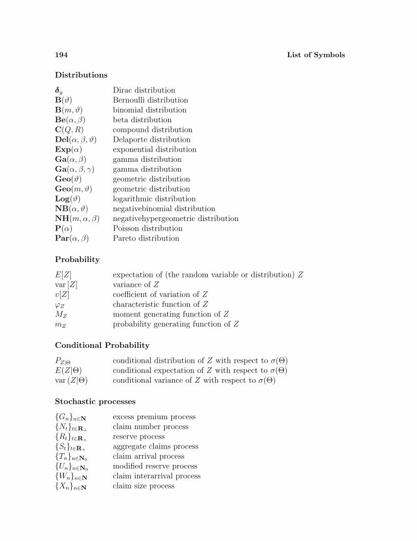
194 List of Symbols
Distributions
δy Dirac distributionB(ϑ) Bernoulli distributionB(m,ϑ) binomial distributionBe(α, β) beta distributionC(Q,R) compound distributionDel(α, β, ϑ) Delaporte distributionExp(α) exponential distributionGa(α, β) gamma distributionGa(α, β, γ) gamma distributionGeo(ϑ) geometric distributionGeo(m,ϑ) geometric distributionLog(ϑ) logarithmic distributionNB(α, ϑ) negativebinomial distributionNH(m,α, β) negativehypergeometric distributionP(α) Poisson distributionPar(α, β) Pareto distribution
Probability
E[Z] expectation of (the random variable or distribution) Zvar [Z] variance of Zv[Z] coefficient of variation of ZϕZ characteristic function of ZMZ moment generating function of ZmZ probability generating function of Z
Conditional Probability
PZ|Θ conditional distribution of Z with respect to σ(Θ)E(Z|Θ) conditional expectation of Z with respect to σ(Θ)var (Z|Θ) conditional variance of Z with respect to σ(Θ)
Stochastic processes
Gnn∈N excess premium processNtt∈R+
claim number processRtt∈R+
reserve processStt∈R+
aggregate claims processTnn∈N0
claim arrival processUnn∈N0
modified reserve processWnn∈N claim interarrival processXnn∈N claim size process
Author Index
A
Adelson, R.M., 125Albrecht, P., 101, 102Aliprantis, C. D., 3Alsmeyer, G., 42Ambagaspitiya, R. S., 126Ammeter, H., 125Azlarov, T. A., 16
B
Balakrishnan, N., 126Bauer, H., 3, 85Bauwelinckx, T., 4Beirlant, J., 170Bichsel, F., 102Billingsley, P., 3, 85Bjork, T., 169Bowers, N. L., 4Bremaud, P., 42Buhlmann, H., 4, 84, 170Burkinshaw, O., 3
C
Chow, Y. S., 85Cox, D.R., 42Csorgo, M., 170
D
Dassios, A., 169, 170Daykin, C.D., 4DeDominicis, R., 84
Deheuvels, P., 170Delaporte, P. J., 102Delbaen, F., 169DePril, N., 126Derron, M., 102DeVylder, F., 126, 169, 170Dickson, D.C.M., 170Dienst, H.R., 154Dubourdieu, J., 101, 102
E
Embrechts, P., 170
G
Galambos, J., 16Gerathewohl, K., 154Gerber, H.U., 4, 101, 102, 125, 126, 169Goovaerts, M. J., 4, 124, 126Grandell, J., 41, 42, 101, 169, 170Gurland, J., 125Gut, A., 42, 170
H
Haezendonck, J., 126, 169Heilmann, W.R., 4Helbig, M., 4Heller, U., 101Helten, E., 1Herkenrath, U., 170Hesselager, O., 125Hickman, J. C., 4
196 Author Index
Hipp, C., 4, 126Hofmann, M., 101
I
Isham, V., 42
J
Janssen, J., 84Jewell, W. S., 125Johnson, N. L., 125, 175, 179Jones, D.A., 4
K
Kaas, R., 4, 124, 126Kallenberg, O., 42Karr, A. F., 42Kemp, A.W., 175Kerstan, J., 41, 42Kingman, J. F.C., 42Kling, B., 126Kluppelberg, C., 170Konig, D., 42Kotz, S., 16, 125, 175, 179Kupper, J., 1, 102
L
Lemaire, J., 102Letta, G., 42Lin, X., 125Lundberg, O., 101, 124
M
Mammitzsch, V., 84, 170Mathar, R., 42Matthes, K., 41, 42Mecke, J., 41, 42Michel, R., 4, 125, 126Mikosch, T., 170Milbrodt, H., 4Møller, C.M., 170
N
Nesbitt, C. J., 4Neveu, J., 42, 170Nollau, V., 84Norberg, R., 4
P
Panjer, H.H., 4, 124, 125, 126, 171Pentikainen, T., 4Pesonen, M., 4Pfeifer, D., 42, 101
Q
Quenouille, M.H., 124
R
Reiss, R.D., 42Resnick, S. I., 42Rhiel, R., 124, 169Runnenburg, J. T., 124Ruohonen, M., 102
S
Scheike, T.H., 126Schmidli, H., 170Schmidt, K.D., 101, 170Schmidt, V., 42Schroter, K. J., 125, 126Seal, H. L., 101, 170Shumway, R., 125Sobrero, M., 126Steinebach, J., 170Sterk, H. P., 1, 154Stormer, H., 84, 154Straub, E., 4Sundt, B., 4, 84, 101, 125, 126
Author Index 197
T
Teicher, H., 85Teugels, J. L., 170Thorin, O., 170Thyrion, P., 102Troblinger, A., 1, 102
V
Van Heerwaarden, A. E., 4Veraverbeke, N., 170Villasenor, J. A., 170Volodin, N. A., 16
W
Wang, S., 125Watanabe, S., 42Wikstad, N., 170Willmot, G. E., 4, 124, 125, 126, 171Wolfsdorf, K., 4Wolthuis, H., 4
Subject Index
A
abstract portfolio, 100adjustment coefficient, 164admissible pair, 45aggregate claims amount, 103, 109aggregate claims process, 103Ammeter transform, 114
B
Bernoulli distribution, 176Bernoulli process, 40beta distribution, 179beta function, 171binomial criterion, 88binomial distribution, 176binomial process, 40binomial risk process, 132bounded stopping time, 161
C
canonical filtration, 25Cantelli’s inequality, 113Chapman–Kolmogorov equations, 46characteristic function, 174claim amount, 103claim arrival process, 6claim event, 6claim interarrival process, 6claim measure, 8claim number, 17, 109claim number process, 17claim severity, 103
claim size process, 103coefficient of variation, 173compound binomial distribution, 111compound distribution, 109compound negativebinomial
distribution, 111compound Poisson distribution, 109compound Poisson process, 107conditionally independent
increments, 86conditionally stationary
increments, 86contagion, 78, 82, 83, 95continuous distribution, 179continuous time model, 9convolution, 175counting measure, 172Cox process, 170
D
decomposition of a claim sizeprocess, 137
decomposition of a Poissonprocess, 133
decomposition of a Poisson riskprocess, 137
degenerate distribution, 172Delaporte distribution, 176DePril’s recursion, 123Dirac distribution, 172discrete distribution, 175discrete time model, 9disjoint familiy, 4
Subject Index 199
distribution, 172doubly stochastic Poisson process, 170
E
Erlang distribution, 180essential infimum, 157estimation, 98exceptional null set, 6, 17excess of loss reinsurance, 108excess premium process, 158expectation, 173experience rating, 101explosion, 7, 10, 75exponential distribution, 180
F
failure rate, 50filtration, 25finite expectation, 173finite moment, 173finite time ruin probability, 170Fourier transform, 174
G
gamma distribution, 180gamma function, 171generalized binomial coefficient, 172geometric distribution, 176
H
heavy tailed distribution, 170homogeneous claim number process, 47homogeneous Poisson process, 23
I
increasing, 4increment, 20, 105independent increments, 23, 105inhomogeneous Poisson process, 56initial reserve, 155
insurer’s portfolio, 100intensity, 49, 56
K
Kolmogorov’s inequality, 164
L
layer, 132Lebesgue measure, 172life insurance, 9lifetime, 9logarithmic distribution, 177Lundberg’s binomial criterion, 88Lundberg’s inequality, 165
M
Markov (claim number) process, 44martingale, 25maximal inequality, 161memoryless distribution, 13mixed binomial process, 92mixed claim number process, 86mixed Poisson process, 87modified reserve process, 158moment, 173moment generating function, 174multinomial criterion, 23, 60, 87multiple life insurance, 9
N
negative contagion, 82, 83negativebinomial distribution, 177negativehypergeometric distribution, 178net premium, 160nondegenerate distribution, 172number of claim events, 107number of claims, 17number of claims occurring at a claim
event, 107number of large claims, 108
200 Subject Index
number of occurred claims, 107, 108number of reported claims, 107
O
occurrence time, 7operational time, 76
P
Panjer’s recursion, 122Pareto distribution, 180partition, 4Pascal distribution, 178point process, 41Poisson distribution, 178Poisson process, 23Poisson risk process, 137Polya–Eggenberger distribution, 178Polya–Lundberg process, 93positive, 4positive adapted sequence, 164positive contagion, 78, 82, 95prediction, 38, 39, 97, 98premium income, 155premium intensity, 155priority, 108probability generating function, 174
R
regular claim number process, 48reinsurance, 108renewal process, 42reserve process, 155risk process, 127ruin, 158ruin problem, 156
S
safety loading, 160semi–Markov process, 84sequence of intensities, 49
single life insurance, 9stationary increments, 23, 105stopping time, 161structure distribution, 86structure parameter, 86submartingale, 25superadjustment coefficient, 164supermartingale, 25superposition of claim size
processes, 148superposition of Poisson processes, 141superposition of Poisson risk
processes, 149survival function, 13
T
tail probability, 113thinned binomial process, 108thinned claim number process, 107, 128thinned claim size process, 130thinned Poisson process, 108thinned risk process, 130, 132time of death, 9total number of claims, 107transition probability, 46transition rule, 45
V
variance, 173variance decomposition, 86
W
waiting time, 7Wald’s identities, 111
X
XL reinsurance, 108
Z
zero–one law on explosion, 10, 75