lifecycle carbon footprint analysis of transportation
TRANSCRIPT

Report # NJ-PL-2011-01
Lifecycle Carbon Footprint Analysis of Transportation Capital Projects
FINAL REPORT June 30, 2011
Submitted by:
Robert B. Noland Christopher S. Hanson
Alan M. Voorhees Transportation Center
Edward J. Bloustein School of Planning and Public Policy Rutgers University
NJDOT Research Project Manager Jamie DeRose
In cooperation with
New Jersey Department of Transportation

DISCLAIMER STATEMENT
The contents of this report reflect the views of the authors who are responsible for the facts and the accuracy of the data presented herein. The contents do not necessarily reflect the official views or policies of the New Jersey Department of
Transportation or the Federal Highway Administration. This report does not constitute a standard, specification, or regulation.

TECHNICAL REPORT STANDARD TITLE PAGE
1. Report No. 2.Government Accession No. 3. Recipient’s Catalog No. NJ-PL-2011-01
4. Title and Subtitle 5. Report Date
Lifecycle Carbon Footprint Analysis of Transportation Capital Projects
June 30, 2011 6. Performing Organization Code
7. Author(s) 8. Performing Organization Report No.
Robert B. Noland and Christopher S. Hanson
9. Performing Organization Name and Address 10. Work Unit No.
Alan M. Voorhees Transportation Center Rutgers University 33 Livingston Ave, New Brunswick, NJ 08901
11. Contract or Grant No.
12. Sponsoring Agency Name and Address 13. Type of Report and Period Covered New Jersey Department of Transportation PO 600 Trenton, NJ 08625
14. Sponsoring Agency Code
15. Supplementary Notes 16. Abstract This report documents the development of GASCAP, the Greenhouse Gas Analysis System for Transportation Capital Projects. The report provides extensive detail on the assumptions underlying the emissions factors for materials, construction equipment, and preliminary work on a life-cycle maintenance module. Appendices incude a review of methods for incorporating the effects of induced travel demand into a sketch planning tool, plus additional documentation for various elements of GASCAP. A user guide is also included as are a selection of case studies that were conducted to provide initial tests of the software. Further research directions to extend the usability of GASCAP are also included.
17. Key Words 18. Distribution Statement
life-cycle analysis; greenhouse gases; emissions; construction projects; asphalt; concrete; transit
19. Security Classif (of this report) 20. Security Classif. (of this page) 21. No of Pages 22. Price
Unclassified Unclassified
Form DOT F 1700.7 (8-69)

ii
iii
ACKNOWLEDGEMENTS
The following students played an integral role in the development of this project. Karthik Rao Cavale provided detailed research assistance in developing inputs for bid sheet items and estimating GHG emissions from process fuels, Patrick Brennan provided background research on components of road projects and roadway maintenance. Jonathan Hawkins was our master programmer whose skill at designing and integrating the information was essential. We also thank Harold Mulleavey at NJ Transit for providing access to data sources and providing case study information. Our advisory board, led by our project manager Jamie DeRose included Andy Swords, Dave Gillespie (from NJ Transit) and Liz Semple and Joe Carpenter (from NJ DEP). Monica Mazurek and Claudia Knezek participated in early discussions in formulating this project. We thank all for the guidance and input they provided for this project.

iv
v
TABLE OF CONTENTS Page
Executive summary ........................................................................................................ i Introduction ................................................................................................................... 1 Review of energy and material inputs ......................................................................... 3
Key Models Used for Estimating Emissions .......................................................... 4 Process Fuels ............................................................................................................ 5
GREET Models ...................................................................................................... 6 Electricity ................................................................................................................... 9 Aggregates .............................................................................................................. 12
The Asphalt GHG Emissions Model .................................................................. 15 Cement and Concrete ............................................................................................. 25
Manufacturing Process ...................................................................................... 26 GHG Emissions ................................................................................................... 27 Alternative Technologies in Cement and Carbon sequestration .................... 28
Iron and Steel .......................................................................................................... 29 Manufacturing Process ...................................................................................... 30 Alternative Technologies in Steel Making ........................................................ 33
Transportation of Construction Materials and Disposal ..................................... 33 Other Materials ........................................................................................................ 34
Review of Life-cycle Construction Equipment Emissions ...................................... 36 NONROAD – Direct Emissions .............................................................................. 37
Spark Ignition Emission Standards Implementation ....................................... 37 Compression Ignition Emission Standards Implementation .......................... 38 Modeling Approach ............................................................................................ 42 NONROAD Model Basics ................................................................................... 46
Adjustments to NONROAD GHG Definitions ........................................................ 49 GREET Model – Upstream Emissions ................................................................... 53
Fossil Fuels Modeled in NONROAD .................................................................. 54 Biofuels ............................................................................................................... 56 Gasoline and Alternatives. ................................................................................. 60 Low Sulfur Diesel and Alternatives. .................................................................. 61
Procedure for Building GASCAP Dataset ............................................................. 62 GASCAP Dataset Inputs and Outputs ................................................................... 63
Review of Maintenance and Rehabilitation Procedures for Roadways and Bridges ...................................................................................................................................... 64
Prediction of Optimum Timing of Maintenance and Rehabilitation Activities ... 65 How LCCA Works ............................................................................................... 66 LCCA Procedure for Pavement ......................................................................... 68 LCCA Procedure for Bridges ............................................................................. 69
GASCAP Approach to Lifetime Maintenance and Rehabilitation ....................... 69 Maintenance and Rehabilitation of Roadways ..................................................... 70
Rigid Pavement Preventive Maintenance ......................................................... 70 Rigid Pavement Corrective Maintenance ......................................................... 70 Rigid Pavement Rehabilitation .......................................................................... 71

vi
Rigid Pavement Reconstruction ........................................................................ 72 Flexible Pavement Preventive Maintenance ..................................................... 72 Flexible Pavement Corrective Maintenance ..................................................... 73 Flexible Pavement Rehabilitation ...................................................................... 73 Flexible Pavement Reconstruction ................................................................... 74 Flexible-over-Rigid Pavement Preventive Maintenance .................................. 75 Flexible-over-Rigid Pavement Corrective Maintenance .................................. 75 Flexible-over-Rigid Rehabilitation ..................................................................... 75 Flexible-over-Rigid Reconstruction .................................................................. 76 Rigid or Flexible-over-Rigid Pavement Widening ............................................ 76 Flexible or Flexible-over-Rigid Pavement Widening ........................................ 76 Flexible Shoulder Preventive Maintenance ...................................................... 77 Flexible Shoulder Corrective Maintenance ...................................................... 77 Flexible Shoulder Rehabilitation ....................................................................... 77
Maintenance and Rehabilitation of Bridges .......................................................... 77 Abutments ........................................................................................................... 78 Approach Slabs .................................................................................................. 79 Arch Bridges ....................................................................................................... 80 Backwalls ............................................................................................................ 81 Beams .................................................................................................................. 82 Bearings .............................................................................................................. 82 Culverts ............................................................................................................... 83 Decks ................................................................................................................... 84 Piers ..................................................................................................................... 88 Slab Bridges ........................................................................................................ 89 Stream beds ........................................................................................................ 90
Incorporation of Maintenance and Rehabilitation into the GASCAP Tool ......... 90 Forecasting Carbon Emissions Using models that Account for Induced Travel .. 91
Summary .................................................................................................................. 91 Introduction ............................................................................................................. 93 Underlying Economic Theory and Behavioral Factors ........................................ 93 Empirical Research Evidence and Forecasting Methods .................................... 98
Aggregate Multivariate Regression Models ..................................................... 99 Facility-Specific Studies .................................................................................. 102 Disaggregate Data Analysis ............................................................................ 104 Disaggregate Regional Travel Demand Models and Land Use Modeling .... 105 Sketch Planning Models .................................................................................. 107
Forecasting and Estimating CO2 Emissions ...................................................... 108 Conclusions .......................................................................................................... 110
Conclusions and Further Research Needs ............................................................. 112 Materials module ................................................................................................... 112 Equipment module ................................................................................................ 112 Life-cycle maintenance......................................................................................... 112 Staging module ..................................................................................................... 113 Lighting module .................................................................................................... 113 Rail module ............................................................................................................ 113
vii
Emissions coverage ............................................................................................. 113 Updating procedures ............................................................................................ 113 Future technologies .............................................................................................. 114 Induced travel module .......................................................................................... 114 Training, testing and feedback ............................................................................ 114
APPENDIX A. Spark Ignition Engines ...................................................................... 115 APPENDIX B. Compression Ignition Engines ......................................................... 125 APPENDIX C. Project Model Results ....................................................................... 133 APPENDIX D. Cool Pavement Technology ............................................................. 177
Background Information: ..................................................................................... 177 Asphalt Technology .............................................................................................. 177 Cement Technology .............................................................................................. 178 Porous Pavements ................................................................................................ 179 Considerations ...................................................................................................... 179 Applications .......................................................................................................... 180
APPENDIX E. Emissions of HFC-134A from Mobile Air Conditioning Systems .. 181 APPENDIX F. Documentation of Materials Calculations ........................................ 183
General Note .......................................................................................................... 183 Subbase, Base and Surface Courses ............................................................. 184 Bridges and Structures .................................................................................... 185 Miscellaneous Items and Utilities .................................................................... 190
APPENDIX G. Data and Assumptions for Rail Capital Projects ............................ 197 The Components of Track .................................................................................... 198
Rail ..................................................................................................................... 198 Ties .................................................................................................................... 199 Joint Bars .......................................................................................................... 201 Ballast ................................................................................................................ 201 Anchors and Other Miscellaneous Items ....................................................... 202 Assumptions for an Average Mile of Track .................................................... 202 Grade ................................................................................................................. 203
Other Components of Rail Systems .................................................................... 204 Passenger Station Assumptions ......................................................................... 205
Parking Facilities .............................................................................................. 205 Estimation of Material and Electricity Emission Factors ................................... 207
Brick and Soil .................................................................................................... 209 Copper and Aluminum ..................................................................................... 210 Wood as Plywood ............................................................................................. 210 Concrete ............................................................................................................ 211 Asphalt .............................................................................................................. 211 Creosote Treated Timber ................................................................................. 211
Conclusion and Summary .................................................................................... 215 APPENDIX H: GASCAP CASE STUDIES ................................................................. 219
Introduction ........................................................................................................... 219 Contract 001093740: Grove Street (CR623) over Route 46, Clifton City, Passaic County ................................................................................................................... 220

viii
Contract 135083070: Route 9 over Main Street, Bridge Superstructre Replacement, Township of Woodbridge, Middlesex County ............................ 221 Contract 003048072: Route US 22 Resurfacing and County Route 519 Intersection Improvements, from Phillipsburg Mall Entrance to Vicinity of Greenwich .............................................................................................................. 222 Contract 045093060: Route 1 & 9 North Avenue to Haynes Avenue Resurfacing, Mill and pave, City of Newark and Elizabeth (Essex and Union Counties) ...... 222 Lessons learned from case studies .................................................................... 223
APPENDIX I: Rail Case Studies ................................................................................ 269 New Jersey Transit Commuter Lines .................................................................. 269 New Jersey Transit Bid-sheets ............................................................................ 275 Conclusions .......................................................................................................... 276
APPENDIX J: References ......................................................................................... 279
ix
LIST OF FIGURES
Page Figure 1. Latent and Specific Heat for Drying and Heating Aggregate and Binder.
........................................................................................................................... 16 Figure 2. Inelastic travel demand and exogenous growth in travel ........................ 94 Figure 3. Elastic travel demand and exogenous growth in travel ........................... 95 Figure 4. Distribution of Benefits of Accessibility Increases .................................. 97 Figure 5. Average Annualized Leak rate by Model Year Bin and Overall ............. 182 Figure 6. Subsystem Contribution to Total GHG Emissions (GWP) – Morristown
Line. ................................................................................................................. 271 Figure 7. Subsystem Contribution to Total GHG Emissions (GWP) – Princeton
Line. ................................................................................................................. 272 Figure 8. Subsystem Contribution to Total GHG Emissions (GWP) – Pascack
Valley Line. ...................................................................................................... 273 Figure 9. Subsystem Contribution to Total GHG Emissions (GWP) – Montclair
Line. ................................................................................................................. 273 Figure 10. Subsystem Contribution to Total GHG Emissions (GWP) – Bergen
County Line. .................................................................................................... 274

x

xi
LIST OF TABLES
Page Table 1. CO2 Equivalence for GWRA Defined Greenhouse Gases ........................... 2 Table 2. Materials Covered by Principal Source. ........................................................ 4 Table 3. GHG Emissions of Process Fuels in g/MMBtu. ............................................ 8 Table 4. Mix of Energy Sources for Electricity Production in the United States and
the Northeast US. ............................................................................................. 10 Table 5. GHG Emission factors for Electricity Production in the United States and
the Northeast US. ............................................................................................. 11 Table 6. GHG Emissions from Limestone and Crushed Rock Production in the
United States 1997. ........................................................................................... 13 Table 7. Fugitive Asphalt Emissions Estimation Method. ....................................... 18 Table 8. Upstream, Combustion, and Fugitive Emissions from HMA and Five WMA
Binders .............................................................................................................. 20 Table 9. Fugitive emissions from use of cutback asphalt. ...................................... 25 Table 10. Concrete GHG Emissions Assuming 12% Cement, 82% Aggregates, and
6% Water. .......................................................................................................... 28 Table 11. GREET Vehicle Cycle Model Emission Factors for Steel. ....................... 32 Table 12. New Technologies in Steel Making ........................................................... 33 Table 13. Plastics, Rubber, Galvanizing Material, and Aluminum Emission
Factors. ............................................................................................................. 35 Table 14. Fertilizer and Herbicide Inputs ................................................................... 35 Table 15. Compression Ignition Emission Standards--NONROAD. ........................ 40 Table 16. Models Used to Estimate GHG Emissions ................................................ 44 Table 17. Adjustments to Zero-Hour Steady State Rates. ....................................... 48 Table 18. Upstream GHG Emissions for Standard Fuels Modeled in NONROAD. . 55 Table 19. Upstream GHG Emissions for Ethanol from Biomass Feedstocks. ....... 56 Table 20. Upstream Emissions from Gasoline, Ethanol, and Blends. .................... 60 Table 21. Upstream Emissions from Low Sulfur and Alternative Diesel Fuels. .... 62 Table 22. Estimated Parameter Estimates from Induced Travel Regression Models
......................................................................................................................... 100 Table 23. Estimates using travel demand models. ................................................. 105 Table 24. Steady State Emissions from Spark Ignition Engines ........................... 115 Table 25. Transient Activity Factors for Spark Ignition Engines........................... 118 Table 26. Deterioration Factors for Spark Ignition Engines. ................................. 121 Table 27. Zero-Hour, Steady-State Emissions from Compression Ignition Engines.
......................................................................................................................... 125 Table 28. Transient Activity Factors for Compression Ignition Engines. ............. 128 Table 29. Compression Ignition Deterioration Factors. ......................................... 131 Table 30. Direct Emissions – 2010 ........................................................................... 133 Table 31. Upstream Emissions – 2010 ..................................................................... 155 Table 32. Summary of Vehicle Leak Rate Estimates (grams/year) ........................ 181 Table 33. Inlet geometry ........................................................................................... 193 Table 34. Inputs for One Mile of 100 lb Track with Continuous Rail. .................... 203 Table 35. Material Inputs of Rail Passenger Stations. ............................................ 206

xii
Table 36. Material Inputs for One Parking Space of Garage Parking. ................... 206 Table 37. GHG Emissions of Process Fuels in g/MMBtu. ...................................... 208 Table 38. Material and Electricity Emission Factors .............................................. 209 Table 39. Concrete GHG Emissions Assuming 12% Cement, 82% Aggregates, and
6% Water. ........................................................................................................ 212 Table 40. GHG Emission Factors for Creosote Pressure Treated Timber Railroad
Ties .................................................................................................................. 215 Table 41. Estimates of GHG Emissions for Rail System Components. ................ 216 Table 42. GHG Emissions from Five New Jersey Transit Commuter Rail Lines. 270 Table 43. Ranges of Estimated GWP for Electrified and Non-Electrified NJT
Commuter Rail Systems. ............................................................................... 275
i
EXECUTIVE SUMMARY
This report summarizes the development of the GASCAP software for analyzing the life-cycle greenhouse gas (GHG) emissions of transportation capital construction projects. GASCAP is a spreadsheet-based tool that allows users to input information directly from NJDOT project bid sheets. Additional information must be entered for specific equipment used during the project. One-time maintenance projects that are specified within bid sheets may also be evaluated for their greenhouse gas emissions. Additional modules of GASCAP allow input of information on recycled materials used in pavements, assumptions on how the project will be staged, an assessment of alternative lighting, and a module for assessing GHG emissions from rail projects. The software is designed to be easy to use. Simple documentation is provided that guides users through each module of the software. GASCAP provides life-cycle emissions estimates for the major GHGs. These include carbon dioxide (CO2), methane (CH4), nitrous oxide (N2O), and black carbon (BC). We also include estimates for the oxidation to CO2 of volatile organic compounds (VOC) and carbon monoxide (CO). The model outputs estimates of both direct emissions and upstream emissions. The latter are primarily due to the process fuels used for material production and electricity generation. This also includes the emissions associated with mining and processing aggregate materials, which are an input to both asphalt and concrete production. Road and bridge construction primarily use three materials: asphalt, concrete, and steel. For asphalt a temperature dependent estimate that spans the range of asphalt types from Hot Mix Asphalt to more carbon efficient Warm Mix Asphalt was developed. This allows users to estimate the difference in emissions from using these mixes of asphalt. For concrete we distinguish the various components of production, including the chemical release of CO2 that occurs in the production of cement. GHG emissions from steel production are also broken down into various components that represent different stages of the production process. These are the three principal materials that are used in most construction projects. Additional materials that are included are copper (mainly for catenary rail systems) and aluminum. Many small components are included in GASCAP. The model includes over 1000 individual bid sheet items, such as pipes for water, gas, and sewage, and drainage structures, and slope and channel protection, among others. Formulas based on the geometry of specific items have been calculated to provide estimates of material volume in the appropriate units for each item. These are easily input by the user using bid sheet numbers.

ii
GASCAP uses existing information on both direct and upstream emissions factors derived from existing sources of data, determined by the US Environmental Protection Agency (EPA), the US Department of Energy (DOE), and other research efforts. Our main sources are the AP-42 emissions factors compiled by EPA, the GREET life-cycle analysis models developed by the Argonne National Laboratory (ANL) for DOE, the PaLATE model developed at the University of California with support from CalTrans and USDOT, the GreenDOT model developed by the NCHRP for lighting emissions factors, and EPA emission models for on-road and non-road vehicles (MOVES and NONROAD). These sources are supplemented with academic sources and our own estimates and assumptions based on a variety of published sources. The first two modules of GASCAP are a materials module and an equipment module. The materials module is input using bid sheet information while the equipment module requires the specification of construction equipment used on the project. The recycling module calculates off-sets to emissions based on the use of recycled materials in pavements and concrete. It is assumed that these materials would not be used elsewhere and thus the benefit of using them is the displacement of other materials used as aggregate in paving materials and concrete. GASCAP includes a module that allows the input of project staging assumptions. The location of the project is used as a basis to estimate the distance that materials and people are transported to the site, and the movement of construction equipment on and off-site if this is a part of the staging strategy. Assumptions are also input on lighting requirements for night work. A lighting module is included that allows the estimate of emissions from different lighting types and power ratings of lamps. Assumptions must be input on the expected number of years of operation. These factors are taken from the GreenDOT model developed for an NCHRP project. GASCAP includes a rail module for NJ Transit capital projects. The model uses a bottom-up approach to calculate emissions from tracks, catenary equipment, and parking facilities, to the greatest extent possible. Other components are based on averages derived from other published estimates for specific rail systems. The lifecycle maintenance module of GASCAP is not yet completed. This will require additional work and the use of data from NJDOT currently being analyzed by another project. The intent is to link the recommended maintenance procedures to capital projects and calculate the lifecycle emissions from those maintenance activities over the lifetime of the project.

iii
This final report documents the assumptions and sources of the data underlying the GASCAP model. The report serves primarily as a reference manual. A user guide for the software is also included. As part of this project we also included a review of techniques to estimate the induced travel from new project construction. Implementation of an approach to do this was not included in the scope of this project. Our review identified existing techniques that might be suitable for developing into a sketch planning tool using New Jersey data. Finally, various items of additional work are identified for the GASCAP tool. In particular the version delivered is in beta and requires testing by NJDOT staff to determine any problems with format, data, and structure, as well as to identify any major omissions. No training has been completed for staff, however, the software is designed to be very user-friendly.

1
INTRODUCTION
The Carbon Footprint Project is part of the State of New Jersey’s effort to substantially reduce GHG emissions from all sources within the state and from electricity consumed in New Jersey but produced out of state, according to the Global Warming Response Act (GWRA), approved July 6, 2007. The GWRA defines GHG as carbon dioxide (CO2), methane (CH4), Nitrous Oxide (N2O), hydrofluorocarbons (HFC), perfluorocarbons (PFC), and sulfur hexafluoride (SF6), as well as any other gas or substance that the New Jersey Department of Environmental Protection (NJDEP) determines to be a contributor to global warming. These gases are recognized nationally (EPA 2009b) and internationally (Climate Registry 2008, IPCC 2009) as the principal contributors to global warming. These gases are referred to as direct GHG in the Environmental Protection Agency (EPA) inventory (EPA 2009b). Indirect GHGs may have greenhouse properties, but are not stable in the atmosphere. Carbon monoxide (CO), and volatile organic compounds (VOC) but not methane, are reactive enough that they generally oxidize quickly to CO2. EPA equipment modeling uses this assumption (EPA 2004b). Other nitrogen oxides (NOX) are mostly transformed before they reach the upper troposphere and probably do not contribute appreciably to global warming (Wayne 1991). Sulfur dioxide (SO2) oxidizes in weeks and precipitates out as acid rain, but is a minor factor in global warming. GHG emissions may be measured in CO2 equivalents (CO2e) or global warming potential factors (GWP), which are synonymous. A molecule of SF6 has the global warming potential of 23,900 molecules of CO2, as shown in Table 1. CO2 is the principal product of combustion, and other chemical processes, such as cement, lime, and iron and steel production, and is taken up by green plants as biomass. VOC and CH4 are usually fugitive emissions from energy production and waste disposal (Wang 1996). N2O emissions are produced from adipic and nitric acid production and fertilizer use. HFCs are used mostly in refrigeration and air conditioning (IPCC 2000). PFCs are used primarily in some aluminum and semiconductor manufacturing processes (IPCC 2000). SF6 is used in electricity production and transmission, magnesium production, and semiconductor manufacturing(IPCC 2000). Of these materials only the first three were addressed in the models we reviewed. PFCs, HFCs, and SF6 emissions from transportation projects are not well documented in the literature. GHG emissions are distinguished by source (Climate Registry 2008). This materials review includes combustion emissions from stationary sources such as for electricity generation, boilers, and furnaces. Process emissions that result from physical or chemical processes from manufacturing are also included. Truck per mile GHG emissions are included to account for materials transportation to the job site. Emissions from the processing of fuels are treated as upstream emissions for the fuel and engine oil consumed by construction equipment.

2
Table 1. CO2 Equivalence for GWRA Defined Greenhouse Gases
GHG Name Formula CO2e/GWP Carbon dioxide CO2 1 Methane CH4 21 Nitrous oxide N2O 310 Hydrofluorocarbons Varies 12-11,700 Perfluorocarbons Varies 6,500-7,400 Sulfur Hexafluoride SF6 23,900 Source: (Climate Registry 2008)
To properly compare the GHG emissions a lifecycle approach is used. This means that not only are direct emissions counted, i.e. those caused directly by the processes under the contractors’ control, but also indirect emissions caused by processes not under the contractors’ control (Climate Registry 2008, Greenhalgh et al. 2005, Raganathan et al. 2009). Indirect GHG emissions include upstream emissions, downstream emissions, and electricity generation. Upstream emissions include those associated with the extraction of raw materials or feedstocks in the case of fuels, transportation of these from the extraction to the refining or processing site, refining or processing, and distribution to the job site (Delucchi 2003, Elcock 2007, Horvath 2004a). Downstream emissions include those associated with demolition, and disposal and recycling of spent materials. There is a strong preference in the guidance literature for direct measurement of GHG emissions (Climate Registry 2008)(Ewing, Cervero 2010)(Ewing, Cervero 2010). However, for materials we assume that beyond the ability to specify parameters of materials by placing an order with suppliers, the process of preparing materials is out of the control of contractors. We therefore attempt to account for variation in the types and subtypes of materials regulated by the state and ordered by its contractors, but use the best available approximation for materials available to New Jersey contractors, often from national averages. In this way we attempt to account for extraction, transportation, processing, and distribution of aggregate, asphalt, cement, iron and steel, as well as the fuels, electricity and secondary materials used to process them, in addition to the emissions due to application of the materials. The GASCAP tool accounts for GHG emissions with sensitivity to what a contractor has knowledge and decision-making power over. Based on the information in this review, GASCAP will allow a user to aggregate material inputs based on the volume or weight of materials used and the embodied energy in those materials. GASCAP will allow users to enter volume, dimensions or weight of materials, expected equipment use and maintenance assumptions and from this return lifetime GHG emissions for the project, with exceptions noted in this report. GASCAP is not intended for the calculation of emission inventories, but rather is meant to provide a method for comparing the GHG impacts associated with different construction techniques and different projects. A review of NJDOT capital projects was conducted using an online draft of the NJDOT Statewide Transportation Improvement Program (STIP) for FY 2010-2019 and an online
3
listing published by the Customer Services Department of NJDOT’s Division of Procurement (Forsyth, Krizek & Rodríguez 2009) of highway contracts for construction and maintenance for FY 1996-2010, commonly known as “bid-sheets.” The first document describes itself as inclusive of New Jersey’s transportation program in a single volume (Handy, Cao & Mokhtarian 2006). Programs and projects for NJDOT and NJ Transit are addressed in separate sections. The second source includes itemized individual contracts with bids from all bidders for FY 2009.
REVIEW OF ENERGY AND MATERIAL INPUTS
This section presents assumptions made about energy and material inputs to construction materials for transportation projects for the GASCAP model. Emissions factors for aggregates, asphalt, cement and concrete, and steel are documented. Aggregates are discussed separately from asphalt and concrete because they are used in both. Aggregate production involves primarily extraction and crushing. It is essentially extracted in the same way as limestone, the principal input of cement. Soil and other fill are not addressed because the principal work done in their production is extraction. We develop a model to estimate the process energy used to heat asphalt because of the variety of temperatures now used to heat warm and cold mix asphalt. The model addresses evaporative emissions from cutback asphalts as well. Cement is treated as a single process. There are differences in cement but not in the lime content, which is the principal source of GHG emissions. Differences in mix specifications for asphalt and concrete are based on the ratio of aggregate to binding material. Steel GHG emissions are estimated based on national averages. However, we estimate separately for cast, rolled, and stamped steel products. The principal source of GHG emissions involved with recycling and disposal of pavement are due to transportation of the materials. We draw our boundary at delivery to the recycling plant because the subsequent processing is done on the inputs to other projects. Table 2 lists the materials covered and principal data sources. A brief discussion of gaps in what we can cover is included. We present some emission factors for some additional materials for which emission factors are readily available from the GREET models.

4
Table 2. Materials Covered by Principal Source.
Principal Source Reference Process Fuels
Coal GREET Fuel Cycle (Argonne National Laboratory 2009)
Natural Gas GREET Fuel Cycle (Argonne National Laboratory 2009)
Conventional Gasoline GREET Fuel Cycle (Argonne National Laboratory 2009)
Distillate Fuel Oil GREET Fuel Cycle (Argonne National Laboratory 2009)
Residual Oil GREET Fuel Cycle (Argonne National Laboratory 2009)
LPG GREET Fuel Cycle (Argonne National Laboratory 2009)
Coke GREET Vehicle Cycle (Argonne National Laboratory 2009)
Petroleum Coke GREET Fuel Cycle (Argonne National Laboratory 2009)
Asphalt GREET Fuel Cycle (Argonne National Laboratory 2009)
Electricity GREET Fuel Cycle (Argonne National Laboratory 2009)
Aggregates USDOE publication (BCS 2002a) Asphalt Heating Model Gencore Presentation (Hunt 2010)
Warm Mix American Trade Initiatives paper (D'Angelo et al. 2008)
Fugitive Emissions EPA AP-42 (EPA 1979) Cutback Fugitive Emissions EPA AP-42 (EPA 1979) Cement/Concrete USDOE paper (Choate 2003)
Steel GREET Vehicle Cycle (Argonne National Laboratory 2007)
Other Materials GREET Vehicle Cycle (Argonne National Laboratory 2007)
Key Models Used for Estimating Emissions
The process of estimating emission factors was primarily informed by three sources. These include the Pavement Life-cycle Assessment Tool for Environmental and Economic Effects (PaLATE) model developed at the University of California, Berkeley (Horvath et al. 2007), the The Greenhouse gases, Regulated Emissions, and Energy use in Transportation (GREET) models developed by Argonne National Laboratory (Argonne National Laboratory 2009, Argonne National Laboratory 2007), and the Compilation of Air Pollutant Emission Factors, Volume 1: Stationary Point and Area Sources (AP-42) developed by the EPA Office of Transportation and Air Quality (OTAQ) (EPA 2010a). We also extract information from EPA’s MOVES model for any transportation emissions associated with materials production, in this case for transport

5
to recycling plants. In all cases we attempt to use well established sources but we have supplemented these with additional information or calculations where needed. The PaLATE model estimates life-cycle emissions for concrete and asphalt pavement, base, and fill components for sub-base. This model addresses disposal and recycling of materials from transportation projects, i.e. concrete and asphalt, and allows the user to specify recycled additives for inclusion in concrete and asphalt or fill. PaLATE is somewhat limited in that its scope is limited to pavement, upstream emissions are not addressed, and PaLATE only models conventional diesel fuel. Among GHG only CO2 but not CH4 or N2O are addressed. Asphalt modeling is limited to hot mix, while newer more carbon efficient alternatives such as warm mix and cold mix asphalt are not addressed. The GREET model is a life cycle GHG emissions modeling tool with two components, a fuel cycle model (Argonne National Laboratory 2009) and a vehicle cycle model (Argonne National Laboratory 2007). The Fuel Cycle component (GREET 1.8c) models upstream GHG emissions from the production of a wide variety of fuels that have coal, petroleum, and biomass as their feedstocks. The Vehicle Cycle component (GREET 2.7) estimates upstream GHG emissions for steel and other materials used in the manufacture of automobiles and trucks that are transferable to the material inputs of transportation capital projects. Both models estimate CO2, CH4, and N2O emissions. GREET modeling of CO2 emissions are estimated as emissions resulting directly from combustion. GREET also provides a CO2 estimate that also accounts for oxidation of CO and VOCs in the atmosphere (Burnham, Wang & Wu 2006). This is done by multiplying both by the ratio of the carbon fraction of each to the carbon fraction of CO2. Both models use this method (Argonne National Laboratory 2009, Argonne National Laboratory 2007). AP-42 is a clearing house of emissions factors of varying quality created by EPA (EPA 2010a). Quality assessment for AP-42 is based on a letter grade. An “A” emission factor is based on tests from randomly chosen facilities for which variability is minimal. A “B” emission factor is based on tests that may lack this randomness but expected variability is minimal. A “C” emission factor is based in part on tests that may have questionable or untested methodologies. A “D” emission factor may be based on a small number of facilities or there may be reason to suspect higher variability in the population of facilities. An “E” emission factor is based on tests of poorer quality, based possibly on more non-random selection, where there might be a higher likelihood of variation within the facility population. Emission factors for CH4 and N2O are generally of poorer quality than CO2 emission factors. Where no alternatives could be found, “D” and “E” emission factors have been used. Where possible we have attempted to validate emission factors on the basis of other literature. Process Fuels
In this section we present emission factors for CO2, CH4, and N2O for fuels used in industrial processes for production of asphalt, cement, and steel. We use emission

6
factors from the Argonne National Laboratories GREET Fuel Cycle and Vehicle Cycle models (Argonne National Laboratory 2009, Argonne National Laboratory 2007). This model is the basis for EPA’s recent proposed renewable fuel standard, and is preferred over the AP-42 estimates which do not include CH4 and N20 emissions for some fuels and it does not include upstream emissions. The lifecycle process used in GREET and the fuel pathways by which fuels are produced from feedstocks is briefly discussed. Emission factors are presented for the three greenhouse gases. These processes have also been rated in AP-421 We investigated the use of these for our process fuel emission factors, but found that in general the quality ratings provided in the documentation were not high. Thus, we use the GREET model estimates. GREET Models
For fuels a five stage lifecycle approach is used based on the GREET Fuel Cycle model (Argonne National Laboratory 2009). A similar approach is used by the National Energy Technology Laboratory for an inventory of lifecycle emissions from petroleum based fuels used in the United States (Gerdes, Skone 2008a). Both methods were developed to address lifecycle emissions for fuels consumed in vehicles, including aircraft in the latter case. Both models address emissions that result from combustion of process fuels, related feedstocks, and fugitive or flared emissions. The five stages are listed by ANL and NETL designations: 1. Feedstock extraction / Raw material acquisition. 2. Feedstock transportation, storage, and distribution / Raw material transport 3. Refining / Fuel production 4. Transportation, storage, and distribution to the delivery system / Transport of Fuels
to Refueling Station 5. Consumption / Operation Petroleum is extracted from land and sea-based deposits and transported to refineries by pipeline, ship, truck and rail (Gerdes, Skone 2008a). Petroleum distillation is essentially a three stage cyclical process by which hydrocarbons are separated by their weights (Speight 2007). In the first stage, atmospheric distillation, crude is gradually heated under oxygen poor conditions to extract the lighter hydrocarbons. LPG is extracted at this stage. The second stage is vacuum distillation, in which heavier hydrocarbons including number 2 fuel oil which is equivalent to diesel oil are removed under vacuum conditions. What is left after vacuum distillation is called the residuum, which includes residual fuel oil, waxes, and asphalt binder. Residuum components may be further processed by heating to higher temperatures, which causes the remaining heavy hydrocarbons to break into smaller molecules, which may be subjected again to distillation. Petroleum coke, which has lost its volatile components results from all three
1 Available at http://www.epa.gov/ttnchie1/ap42/.
7
steps described here and is often considered a byproduct to be avoided. However, the residuum may also be deliberately coked (Speight 2007).2 The GREET Fuel Cycle Model (Argonne National Laboratory 2009) defines upstream emissions for each pollutant as the mass of that pollutant in grams per MMBtu (Btu x 106) from combustion and upstream emissions that in turn, went into producing that process fuel based on the quantity used, energy content and emissions rate for each process fuel (Wang, Huang 1999). Fuel consumption is based on an estimation of efficiency which refers to the ratio of energy contained in the fuel to the energy contained in all feedstocks including those lost to fugitive emissions, and process fuels (Wang, Huang 1999, Wang 2008). shows upstream and combustion emissions derived from the GREET model for process fuels, including asphalt which is derived from petroleum. Various default assumptions are built into the GREET Fuel Cycle Model (Argonne National Laboratory 2009) in producing these estimates. GREET Model Defaults and Other Assumptions
Fuel-specific refinery emissions are based on a global petroleum refinery efficiency coefficient, which is the ratio of the energy in finished refinery products to the sum of the energy in the crude, other feedstocks, and process fuels (Wang 2008). Specific refinery energy efficiencies are calculated based on industry rule of thumb assumptions that 60% of all process fuels are used to produce gasoline, 25% are used to produce diesel, and 15% are used to produce all other products. Gasoline accounts for 47.0% of energy content, diesel for 25.7% and all other products are 27.3%. On this basis fuel-specific refinery intensities are 1.28, 0.97, and 0.55 for gasoline, diesel and other products, respectively (Wang 2008). This gives process efficiencies of 87.7%, 90.3%, and 94.3% gasoline, diesel, and other products respectively. Where the Fuel Cycle does not apportion fuel-specific refinery production efficiencies we apportion upstream emissions for each GHG on an energy basis by adding extraction and transportation emissions for crude petroleum in g/MMBtu to the refinery specific emissions, also in g/MMBtu. In this way we estimated the upstream emissions for residual oil, petroleum coke, and asphalt. In the case of asphalt we assumed the same processing as residual oil because both are residua, and corrected for Lower Heating Values (LHV) of 94.2 for residual oil and 85.1 for asphalt (Wang, Lee & Molburg 2004). This correction is further justified by the use of a constant refinery efficiency for all other products in the GREET Fuel Cycle model. Our principal interest in natural gas for purposes of materials production is as both feedstock and fuel for use in stationary industrial boilers. Natural gas is extracted from and recovered from oil and natural gas fields (Wang, Huang 1999). Transmission is generally through pipelines to processing plants. During processing heavier
2 Coking occurs in the petroleum refining process when hydrocarbons are heated to the point that all of the hydrogen is lost leaving essentially pure carbon. For a full explanation of this process see (Speight 2007).
8
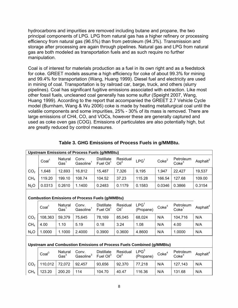
hydrocarbons and impurities are removed including butane and propane, the two principal components of LPG. LPG from natural gas has a higher refinery or processing efficiency from natural gas (96.5%) than from petroleum (94.3%). Transmission and storage after processing are again through pipelines. Natural gas and LPG from natural gas are both modeled as transportation fuels and as such require no further manipulation. Coal is of interest for materials production as a fuel in its own right and as a feedstock for coke. GREET models assume a high efficiency for coke of about 99.3% for mining and 99.4% for transportation (Wang, Huang 1999). Diesel fuel and electricity are used in mining of coal. Transportation is by railroad car, barge, truck, and others (slurry pipelines). Coal has significant fugitive emissions associated with extraction. Like most other fossil fuels, uncleaned coal generally has some sulfur (Speight 2007, Wang, Huang 1999). According to the report that accompanied the GREET 2.7 Vehicle Cycle model (Burnham, Wang & Wu 2006) coke is made by heating metallurgical coal until the volatile components and some impurities, 25% - 30% of its mass is removed. There are large emissions of CH4, CO, and VOCs, however these are generally captured and used as coke oven gas (COG). Emissions of particulates are also potentially high, but are greatly reduced by control measures.
Table 3. GHG Emissions of Process Fuels in g/MMBtu.
Upstream Emissions of Process Fuels (g/MMBtu)
Coal1 Natural Gas1
Conv. Gasoline1
Distillate Fuel Oil1
Residual Oil3 LPG1 Coke2 Petroleum
Coke3 Asphalt3
CO2 1,648 12,693 16,812 15,487 7,326 9,195 1,947 22,427 19,537
CH4 119.20 199.10 108.74 104.52 37.23 115.28 166.54 127.68 109.00
N2O 0.0313 0.2610 1.1400 0.2483 0.1179 0.1583 0.0346 0.3866 0.3154
Combustion Emissions of Process Fuels (g/MMBtu)
Coal1 Natural Gas1
Conv. Gasoline1
Distillate Fuel Oil1
Residual Oil1
LPG1
(Propane) Coke4 Petroleum Coke1 Asphalt4
CO2 108,363 59,379 75,645 78,169 85,045 68,024 N/A 104,716 N/A
CH4 4.00 1.10 5.19 0.18 3.24 1.08 N/A 4.00 N/A
N2O 1.0000 1.1000 2.4000 0.3900 0.3600 4.8600 N/A 1.0000 N/A
Upstream and Combustion Emissions of Process Fuels Combined (g/MMBtu)
Coal3 Natural Gas3
Conv. Gasoline3
Distillate Fuel Oil3
Residual Oil3
LPG3
(Propane) Coke4 Petroleum Coke3 Asphalt4
CO2 110,012 72,072 92,457 93,656 92,370 77,218 N/A 127,143 N/A
CH4 123.20 200.20 114 104.70 40.47 116.36 N/A 131.68 N/A

9
N2O 1.0313 1.3610 3.5400 0.6383 0.4779 5.0183 N/A 1.3866 N/A
Sources: 1. GREET Fuel Cycle Model 1.8c (Argonne National Laboratory 2009). 2. GREET Vehicle Cycle Model 2.7 (Argonne National Laboratory 2007).
3. Our Calculations for Crude Extraction and Refining Share - energy basis from Fuel Cycle model and Summation of Combined Emissions.
4. See subsequent sections for asphalt and steel production. Combustion emissions were not presented for asphalt because it is not a fuel. Combustion emissions for coke were not presented either, because coke as modeled in the GREET 2.7 Vehicle Cycle model (Argonne National Laboratory 2007) is only one component of blast furnace emissions. It will be accounted for as such in the discussion of iron and steel production below. The estimates presented in Table 3 are national averages, but represent the best available information on lifecycle emissions of process fuels. Electricity
Indirect emissions from purchased electricity are required reporting under the Climate Registry’s General Reporting Protocol and the GHG Protocol Project Accounting published by World Business Council for Sustainable Development and the World Resources Institute (Climate Registry 2008, Greenhalgh et al. 2005).GHG emissions from electricity on the grid include those resulting from generation, transmission and distribution. Transmission and distribution emissions are reported as indirect emissions only by electric companies to avoid double counting. Electric power consumers are required only to report generation emissions. The electricity emission factors presented here are used primarily to account for embodied energy in purchased materials. It is assumed that little purchased electricity is used in transportation capital projects. As that is the case transmission and distribution emissions are beyond the scope of this project and general GHG emission factors are called for. GHG emissions from electricity are the sum of emissions from the fuels used to generate power. The GHG emission factors for purchased electricity used here are taken from the GREET 1.8c Fuel Cycle model (Argonne National Laboratory 2009). The Northeast US emission factors are preferred to the emission factors for GHG in the United States as a whole because we assume that materials purchased and applied by contractors in New Jersey are more likely to originate in the Northeast than elsewhere. The Northeast includes New England, New York State, New Jersey, Delaware, and most of Maryland and Pennsylvania (Hirst 2004). Error! Reference source not found. shows the distribution of sources of electricity in the Northeast and the United States as a whole, assuming transmission losses of 8% (Argonne National Laboratory 2009).

10
Table 4. Mix of Energy Sources for Electricity Production in the United States and the Northeast US.
United States Northeast US Residual Oil 1.10% 2.20% Natural Gas 18.30% 21.70% Coal 50.40% 29.90% Nuclear Power 20.00% 33.90% Biomass 0.70% 2.20% Other Sources* 9.50% 10.10% * hydro electric, wind, and geothermal energy are offered as examples. Source: GREET 1.8c Fuel Cycle model (Argonne National Laboratory 2009)

11
Table 5. GHG Emission factors for Electricity Production in the United States and the Northeast US.
United States Northeast US g/kWh g/MMBtu g/kWh g/MMBtu VOC 0.0102 2.988 0.0116 3.394 CO 0.5938 174.047 0.1356 39.745 CH4 0.0130 3.801 0.0122 3.568 N2O 0.0091 2.674 0.0092 2.682 CO2 704 206,399 492 144,113 CO2 (incl. VOC, CO) 705 206,682 492 144,186
Source: GREET 1.8c Fuel Cycle model (Argonne National Laboratory 2009) As a result electricity from the grid in the Northeast has lower GHG emissions per kWh than in the United States as a whole, largely because of its greater reliance on nuclear power and natural gas and lower reliance on coal.

12
shows GHG emission factors from electricity production in the United States and the Northeast. Biomass and clean energy sources such as wind power account for 10% of the US mix and 12% in the Northeast. Aggregates
Aggregates are mineral components added to cement in the production of concrete and are also dried, heated and added to asphalt binder in the production of asphalt. Aggregates may be fine or coarse. Virgin fines are the consistency of sand. Virgin coarse aggregates are crushed stone or gravel. Combined fine and coarse aggregates account for 82% of concrete by weight (Choate 2003). Coarse and fine aggregates make up at least 92% of asphalt by weight if no recycled asphalt pavement (RAP) is used (OTAQ 2004b). AP-42 emissions guidance (EPA 2010a) for fine aggregates and coarse aggregates indicate that particulate matter is the primary emission from extraction of aggregates. CO2 emissions result from equipment use, primarily dryers. As modeled in PaLATE (Horvath et al. 2007) sand and coarse aggregates are input separately but the same emission factor is applied, and the PaLATE model uses the same emission factors for aggregates used for both concrete and asphalt.

13
Table 6. GHG Emissions from Limestone and Crushed Rock Production in the United States 1997.
Production 1.2 Billion tons 1.00E+09 Energy Consumption
Units CO2 CH4 N2O
Coal1 MMBtu g/MMBtu g/ s ton g/MMBtu
g/ s ton g/MMBtu g/ s ton
43 Thousand tons 965,806 110,012 88.542 123.203 0.099 1.031 0.001
Fuel oil2
4 Million bbl. 21,579,600 93,656 1684.219 104.703 1.883 0.638 0.011
Gas
5.4 Billion Cubic Ft. 5,308,200 72,072 318.809 200.197 0.886 1.361 0.006
Gasoline
14.7 Million Gallons 1,706,523 92,457 131.483 113.931 0.162 3.540 0.005 Net Electricity Purchased
4,584 Million kWh 15,681,130 144,186 1884.167 3.568 0.047 2.682 0.035
Total 45,241,259 512,383 4,107.220 545.602 3.077 9.252 0.058
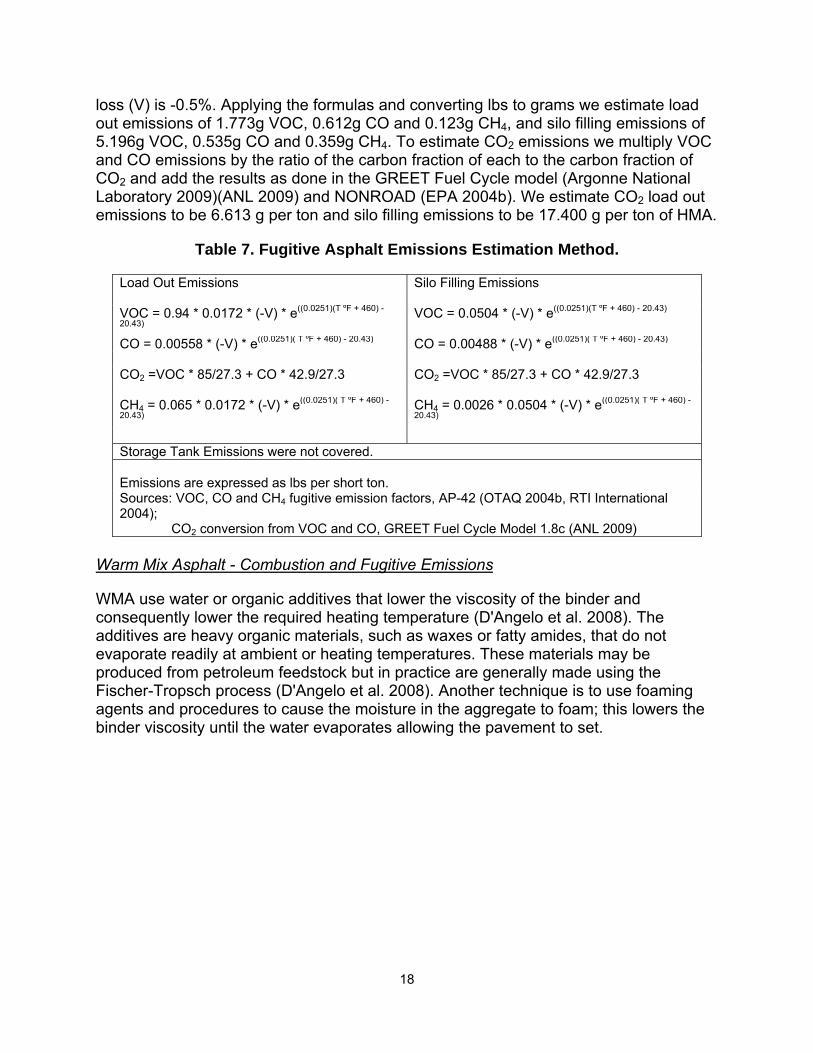
1. Assume Bituminous coal 2. Assume diesel fuel oil Sources: (BCS 2002b) GREET Fuel Cycle Model 1.8c (Argonne National Laboratory 2009). We assume that the extraction of coarse and fine virgin aggregates for asphalt and concrete produce indistinguishable GHG emission factors. An energy and environmental profile of the mining sector prepared for the USDOE equates limestone and crushed rock extraction GHG emissions (BCS 2002b). That study shows total production of limestone and crushed rock of 1.2 billion short tons of material in 1997 and provides a breakdown of energy use by fuel type and electricity use. The results for the entire US are shown in Table 7. We use the AP-42 guidance default assumptions (EPA 2010a, RTI International 2004) to estimate fugitive emissions for one short ton of HMA heated to 325oF with 5% binder by weight. The weight of the binder is 100 lbs. The AP-42 default assumption for volume loss (V) is -0.5%. Applying the formulas and converting lbs to grams we estimate load out emissions of 1.773g VOC, 0.612g CO and 0.123g CH4, and silo filling emissions of 5.196g VOC, 0.535g CO and 0.359g CH4. To estimate CO2 emissions we multiply VOC and CO emissions by the ratio of the carbon fraction of each to the carbon fraction of CO2 and add the results as done in the GREET Fuel Cycle model and NONROAD (EPA 2004b, Argonne National Laboratory 2009). We estimate CO2 load out emissions to be 6.613 g per ton and silo filling emissions to be 17.400 g per ton of HMA.

14
GHG emissions were estimated by converting fuel and electricity consumption by energy type to MMBtu. Using the GREET 1.8c Fuel Model (Argonne National Laboratory 2009) factors for fuel and electricity, we estimate that extraction and processing of a short ton of aggregate results in 4,107 g of CO2, 3.076 g of CH4, and 0.058 g of N2O. These estimates include extraction, transportation, and processing, but not emissions involved in distribution to the job site. Asphalt Asphalt pavement is a mixture of roughly four to eight percent bituminous binder and the balance is course and fine aggregates or recycled material. When mixed, rolled and set the pavement has air voids. Binder is a residual of petroleum refining that consists of the heavier components of crude oil that remain after two stages of distillation. Upstream GHG emissions from the refining process are based on our analysis of process fuel inputs and for aggregate are based on our previous discussion. Direct GHG emissions include products of combustion associated with heating and evaporation and combustion of the binder material. Downstream GHG emissions include those associated with removal and disposal of spent asphalt pavement. GHG reducing technologies in asphalt production focus on recycling and reduced heating requirements. Asphalt fugitive emissions from combustion and evaporation during the production process are minor. A laboratory analysis evaluated with a regression model (Mallick, Bergendahl 2009) showed a strong correlation between CO2 emissions and heating temperature (R2 = 0.976). Heating temperature, the amount of warm mix asphalt (WMA) binder used, and the amount of added asphalt were their independent variables. This is strong evidence that production temperature is a valid and simple modeling approach to estimating GHG emissions for asphalt. Asphalt binder increases pliability and volume at higher temperatures and may shrink and become brittle at lower temperatures (US Army Corps of Engineers 2000). As a liquid, binder is serviceable if it has sufficient viscosity or stiffness to hold its shape at warm ambient temperatures and does not break at cold temperatures under the stress of traffic. Asphalt pavement fails by deforming or cracking. It is referred to as flexible pavement as opposed to concrete, which is known as rigid pavement (Zapata, Gambatese 2005). The lifetime of asphalt pavement is constrained by the oxidation of the binder, which slowly causes the pavement to become less flexible and more brittle. The inputs for GASCAP are similar to those used in the PaLATE model (Horvath et al. 2007). For pavement, the user will specify the length, width, and depth to establish volume. The user will also specify binder proportion, moisture content, and heating temperature and the rating if cutback asphalt is used.3 The defaults are 5% binder at 325oF and 4% moisture content in the aggregate. These defaults are taken from
3 Cutback asphalt refers to binder material that has added hydrocarbon solvents which lower the application temperature. The solvents evaporate after the material is applied, which allows the asphalt to harden. The evaporated solvents must be accounted for as fugitive emissions.

15
industry standards which are discussed below. Volume will be multiplied by density for the binder and aggregates separately. Treatments that do not include aggregates such as tack coats will be entered separately as a volume and converted to weight. Upstream emissions, heating emissions, fugitive emissions, and downstream emissions will be disaggregated. These will be expressed as grams of each GHG and GWP per short ton of material. We develop a method to estimate heating emissions based on the specific temperature needed to heat asphalt. This method will account for upstream and combustion emissions and fugitive emissions. It was necessary to model asphalt production in this way because of the variability of heating requirements and fuel consumption presented by WMA, and this will provide a means to compare the GHG emissions from alternative technologies. The Asphalt GHG Emissions Model
Asphalt is mixed and applied at temperatures high enough to make the mixture malleable without causing it to burn significantly. To accomplish this more economically, additives may be included to lower the viscosity so that the mixture is malleable at lower temperatures. Hot mix asphalt (HMA) is heated to temperatures ranging from 300-325oF (149-163oC) or 302-338oF (150-170oC) (EPA 2010a, Meil 2006, White et al. 2010). Heating asphalt to extremely high temperatures causes the binder to breakdown or crack (Speight 2007). Our GHG emissions model for asphalt has three steps. We address HMA as a reference case and account for GHG reductions from reducing heat inputs. We then account for fugitive emissions from cutback. Hot Mix Asphalt Combustion Emissions.
By one estimate between 70% and 90% of the fuel used to heat asphalt is natural gas and most of the balance is #2 fuel oil (EPA 2010a). Our default assumption is that 80% of the fuel used is natural gas and 20% is fuel oil. A model of energy use in US asphalt production suggests that 8.5% of energy consumed is used for extraction of raw materials and placement, 40% of the energy is used to produce the binder, 48% is used to mix and dry the aggregate and 3.5% is used to store binder at a workable temperature (Zapata, Gambatese 2005). Estimates of upstream emissions vary considerably because of differences in parsing energy use in the extraction and refining of crude petroleum among the fractions (Argonne National Laboratory 2009, Zapata, Gambatese 2005). The energy required to mix and dry one short ton of asphalt with 5% binder is estimated at 318,649 Btu in the United States (Zapata, Gambatese 2005) and 380,179 Btu in Canada (Meil 2006). This difference is not inconsequential but may be explained by variation in moisture content in the aggregate, as demonstrated in Figure 1. Latent and Specific Heat for Drying and Heating Aggregate and Binder.Figure 1. Knowing total energy use and asphalt production in the United States we estimate that the average mix at the national level was 4.75% binder (Zapata, Gambatese 2005). Standard HMA is modeled here on the basis of 5% binder and 95% aggregates with a

16
moisture content of 4%. This ratio is commonly used elsewhere in the literature (Meil 2006, White et al. 2010). The desired moisture content of aggregate before heating is 3% or less, while aggregate used for asphalt production in the United States is often 5% or higher (D'Angelo et al. 2008). We assume a default for aggregate moisture is the average of these two benchmarks of 4%. Our heating model follows the procedure used by Gencor (Hunt 2010). We estimate the energy (Q) required to heat materials as the product of the specific heat value (c), the mass of the material (m) in pounds, and the temperature differential (ΔT) in degrees Fahrenheit. Q = c •m • ΔT The following specific heat values are used:
• c(water) = 1.00 Btu/lb • c(steam) = 0.50 Btu/lb • c(aggregate) = 0.22 Btu/lb
Figure 1. Latent and Specific Heat for Drying and Heating Aggregate and Binder.
0
0.05
0.1
0.15
0.2
0.25
0.3
0.35
50º 75º 100º 125º 150º 175º 200º 225º 250º 275º 300º 325º
Energy Req
uired to Heat One
Sho
rt Ton
of A
spha
lt(M
MBtu)
Temperature in Degrees Fahrenheit‐‐‐‐‐‐‐‐‐‐‐‐‐‐‐‐‐‐‐‐‐‐‐‐‐‐‐‐‐‐‐‐‐‐‐‐‐
Moisture Content of Aggregate
4% 5% 6% 7% 8%

17
The model inputs are heating temperature, binder content, and moisture content of the aggregate. The heating requirements for binder and aggregate are estimated, as is the specific temperature to heat the moisture in the aggregate to the boiling point, the latent heat to evaporate the moisture, and the specific temperature to heat the steam to the target production temperature. The specific temperture for binder is estimated from the average specific heat values at 60oF (16 oC) and 325oF (163 oC) at 0.468 Btu per degree per pound (Abraham 1945). The other assumptions are based on Gencor (Hunt 2010). The latent heat required to evaporate water is 970 Btu per pound. Ambient temperature is 60oF (16 oC). Unless the mixture is not heated above the boiling point of water there is latent heat. Water is heated to a maximum of 212oF (100 oC ) and steam is heated from 212oF (100 oC) to the final heating temperature. Aggregates and binder are heated from ambient temperature to the final heating temperature. Figure 1 shows heating functions for HMA heated from an ambient temperature of 60oF (16 oC ) to a final heating temperature of 325oF (163 oC) with moisture in the aggregate between 4% and 8%. Our model estimates energy use to heat one short ton of HMA with 5% binder and 4% moisture in the aggregate at 216,461 BTU at 100% efficiency. This estimate does not account for waste heat, or the mixing energy. It also does not account for the energy required to maintain binder at a mixing temperature. The American estimate of energy expended was 318,649 Btu per ton (Zapata, Gambatese 2005). The heating required is the ratio of the specific heat calculated at 100% and the observed American average. That ratio is 67.93%. This proportion will be used as a factor to convert heating requirement estimates for HMA, WMA and cutback asphalts to a realistic estimate of energy consumption. Fugitive Asphalt Emissions
When asphalt is heated a small part of the hydrocarbon in the binder oxidizes and lighter components produced during heating evaporate (EPA 2010a). These emissions occur mostly when the heated binder-aggregate mixture, known as asphalt concrete, is removed from the oven--load out emissions--and during silo storage--silo filling emissions. Fugitive emissions also occur when asphalt binder is added to storage tanks. Load out and silo filling emissions are estimated using the method described in Table 7Error! Reference source not found.. We do not have an estimate for storage tank emissions, which is a minor gap in our method. Fugitive emissions were estimated based on the AP-42 guidance (EPA 2010a, RTI International 2004). The model estimates total organic compounds (TOC) and CO as logistic functions of the absolute temperature in degrees Fahrenheit (Rankine scale). For load out emissions, VOCs make up 94% of the TOCs by weight and CH4 makes up 6.5%. (the sum does not add up to 100% due to rounding errors). Virtually all silo filling TOC emissions are VOCs (100%) and CH4 makes up 0.26% of these. VOCs and CO oxidize to CO2 in the atmosphere. Emissions calculated based on Table 7are expressed in lbs per short ton.
We use the AP-42 guidance default assumptions (EPA 2010a, RTI International 2004) to estimate fugitive emissions for one short ton of HMA heated to 325oF with 5% binder by weight. The weight of the binder is 100 lbs. The AP-42 default assumption for volume
18
loss (V) is -0.5%. Applying the formulas and converting lbs to grams we estimate load out emissions of 1.773g VOC, 0.612g CO and 0.123g CH4, and silo filling emissions of 5.196g VOC, 0.535g CO and 0.359g CH4. To estimate CO2 emissions we multiply VOC and CO emissions by the ratio of the carbon fraction of each to the carbon fraction of CO2 and add the results as done in the GREET Fuel Cycle model (Argonne National Laboratory 2009)(ANL 2009) and NONROAD (EPA 2004b). We estimate CO2 load out emissions to be 6.613 g per ton and silo filling emissions to be 17.400 g per ton of HMA.
Table 7. Fugitive Asphalt Emissions Estimation Method.
Load Out Emissions Silo Filling Emissions VOC = 0.94 * 0.0172 * (-V) * e((0.0251)(T ºF + 460) -
20.43) VOC = 0.0504 * (-V) * e((0.0251)(T ºF + 460) - 20.43)
CO = 0.00558 * (-V) * e((0.0251)( T ºF + 460) - 20.43) CO = 0.00488 * (-V) * e((0.0251)( T ºF + 460) - 20.43) CO2 =VOC * 85/27.3 + CO * 42.9/27.3 CO2 =VOC * 85/27.3 + CO * 42.9/27.3 CH4 = 0.065 * 0.0172 * (-V) * e((0.0251)( T ºF + 460) -
20.43) CH4 = 0.0026 * 0.0504 * (-V) * e((0.0251)( T ºF + 460) -
20.43)
Storage Tank Emissions were not covered. Emissions are expressed as lbs per short ton. Sources: VOC, CO and CH4 fugitive emission factors, AP-42 (OTAQ 2004b, RTI International 2004); CO2 conversion from VOC and CO, GREET Fuel Cycle Model 1.8c (ANL 2009)
Warm Mix Asphalt - Combustion and Fugitive Emissions
WMA use water or organic additives that lower the viscosity of the binder and consequently lower the required heating temperature (D'Angelo et al. 2008). The additives are heavy organic materials, such as waxes or fatty amides, that do not evaporate readily at ambient or heating temperatures. These materials may be produced from petroleum feedstock but in practice are generally made using the Fischer-Tropsch process (D'Angelo et al. 2008). Another technique is to use foaming agents and procedures to cause the moisture in the aggregate to foam; this lowers the binder viscosity until the water evaporates allowing the pavement to set.

19
displays the upstream, combustion and fugitive emissions associated with five WMA products from a review of European practice (D'Angelo et al. 2008) including HMA for reference. Upstream emissions for binder and aggregates are not included because they are not sensitive to heating temperatures, but are included in GASCAP.

20
Table 8. Upstream, Combustion, and Fugitive Emissions from HMA and Five WMA Binders
HMA - reference - 325oF (163 oC) Sasobit -Fischer-Tropsch wax - 289oF (143 oC)
Upstream fuel
Combustion
Fugitive Upstream fuel Combustion Fugitive
g/ton g/ton g/ton g/ton g/ton g/ton CO2 4,075.324
19,416.812 24.013 CO2 3,741.145 17,824.625 9.728
CH4 55.412 0.282 0.482 CH4 50.869 0.259 0.195
N20 0.079 0.295 N/A N20 0.073 0.270 N/A
LEA - foaming agent - 212oF (100 oC) 3E LT or Ecoflex - propietary process - 271oF (133 oC)
Upstream fuel
Combustion
Fugitive Upstream fuel Combustion Fugitive
g/ton g/ton g/ton g/ton g/ton g/ton CO2 3,026.375
14,419.114 1.408 CO2 3,574.056 17,028.532 6.192
CH4 41.150 0.209 0.028 CH4 48.597 0.247 0.124
N20 0.059 0.219 N/A N20 0.070 0.258 N/A
LEAB - foaming agent - 194oF (90 oC) Evotherm - hot aggreate coated with emulsion - 239oF (115oC)
Upstream fuel
Combustion
Fugitive Upstream fuel Combustion Fugitive
g/ton g/ton g/ton g/ton g/ton g/ton CO2 1,511.925 7,203.541 0.896 CO2 3,277.009 15,613.255 2.773 CH4 20.558 0.105 0.018 CH4 44.558 0.227 0.056
N20 0.029 0.109 N/A N20 0.064 0.237 N/A Sources:
1. (D'Angelo et al. 2008) 2. Carbon Footprint asphalt emissions model
Note: Temperature conversions were calculated and not taken from D’Angelo et al. Of the products in

21
, Sasobit and 3E LT include 2%-3% organic compounds. LEA and LEAB include foaming agents that make up less than 1% of the binder material. These materials make up minor proportions of binder (D'Angelo et al. 2008). We have not evaluated the GHG impact of producing these additives. Fugitive emissions are a minor source of GHG emissions from asphalt. HMA fugitive emissions are substantially than less for CO2 emissions than the combined upstream and direct emissions from fuel use. As temperatures decline from 325oF fugitive emissions drop off rapidly.

22
Cutback Asphalt GHG Emissions
Cutback asphalt refers to binder material that has added hydrocarbon solvents that lower the temperature at which the asphalt is applied, by lowering the viscosity. The solvents evaporate after the material is applied, which allows the asphalt to harden. The evaporated solvents must be accounted for as fugitive emissions in addition to emissions from heating. Cutback asphalts are rated by the speed by which they cure (AASHTO 2007). Curing speed is accomplished by varying the density of the added hydrocarbon solvents. The solvents used are 0.7 kg/l for rapid cure (RC) additives, 0.8 kg/l for medium cure (MC) additives, and 0.9 kg/l for slow cure (SC) additives (OTAQ 1979). Asphalt binder has a density of about 1.1 kg/l. It is assumed that 95% of rapid cure cutbacks, 70% of medium cure cutbacks and 25% of slow cure cutbacks evaporate as VOCs. Cutbacks modeled in the AP-42 guidance contain 25%, 35% or 45% solvent (EPA 1979). A VOC emission factor was derived from the AP-42 guidance (EPA 1979). The volume of evaporative VOC emissions is: EFVOC = Solvprop * Solvdens / (Solvprop * Solvdens + (1 - Solvprop) * 1.1) * Emissionsprop where EFVOC is the VOC emission factor; Solvprop is the proportion of solvent in the binder; Solvdens is the density of the sovlents in kg/l; 1.1 kg/l is the density of asphalt; and Emissionsprop is the proportion of solvents that evaporate.

23
shows estimates for VOC emissions and resulting CO2 emissions. It was possible to verify application of the AP-42 formulas by correctly recreating Table 4.5-1 of the AP-42 guidance for cutback asphalt using the formula presented in the guidance (EPA 1979). Applying the formulas in this way makes it possible for GASCAP users to change default solvent density and proportions. This approach is suitable for estimating VOC emissions from cutback with a C rating.

24
shows CO2 emissions on a per gallon and per ton basis estimated from carbon content.

25
Table 9. Fugitive emissions from use of cutback asphalt.
VOC Emissions % of volume lost Solvent Proportion Type of Cutback 25% 35% 45% Rapid cure 17% 24% 33% Medium cure 14% 20% 26% Slow cure 5% 8% 10% Source: AP-42 Section 4.5 (EPA 1979) CO2 Emissions g/gal Solvent Proportion Type of Cutback 25% 35% 45% Rapid cure 1,959 2,743 3,527 Medium cure 1,650 2,310 2,970 Slow cure 663 928 1,193 CO2 Emissions g/ton Solvent Proportion Type of Cutback 25% 35% 45% Rapid cure 469,584 684,810 918,751 Medium cure 385,794 556,397 737,607 Slow cure 151,316 215,956 283,156
Cement and Concrete
Concrete is composed of cement, water, and coarse and fine aggregate. Aggregate is a material such as sand, gravel, crushed stone, etc that provides the shape to concrete. Cement and water combine to form the paste that when dried and hard holds the aggregates together. Cement makes up 7 to 15% of concrete by weight (Marceau, Nisbet & VanGeem 2007). Though a small component, cement accounts for the vast majority of the GHG emissions from production of concrete. This is due to CO2 emissions when cement is heated to temperatures of approximately 2,750oF, which results in conversion of limestone (CaCO3) into lime (CaO) releasing CO2 from the conversion reaction and combustion emissions from the fuel used for heating (EPA 2010a). Cement represents approximately 86% energy consumption in concrete production and between 89% and 96% of CO2 emissions according to two life cycle inventories for the United States (Choate 2003, Marceau, Nisbet & VanGeem 2007). The cement content of concrete has an important impact on the overall GHG emissions and energy consumption of concrete. There are many classifications of cement, however three grades Type I, Type II and Type III, that include cement classified as Type 1/2, account for at least 95% of Portland cement production (FHWA 1999). These three have CaO content of between 61.37% and 61.61% (Clemeña 1972). We model cement as Portland cement because it accounts for nearly all (93%) of US production (Greer, Dougherty & Sweeney 2000) and is favored in the transportation sector. Other types of cement are produced through roughly the same processes and while we do not

26
describe these in detail, we can account for them in the final model through minor modification of the multipliers used for standard Portland cement. Users of GASCAP are asked to input cement content of the mix design and fine and coarse aggregates as virgin aggregates or recycled material, water and additives. The model will separately estimate GHG emissions from the cement, the virgin aggregates and any recycled aggregates. Emissions are based on an inventory of the cement industry done for the US Department of Energy (Choate 2003). Emissions from fuel consumption are based on the GREET Fuel Cycle model (Argonne National Laboratory 2009). Manufacturing Process
Cement production has mechanical and chemical components. The mechanical process involves movement of materials through a cement manufacturing plant from quarry to shipment to construction site. Manufacturing sites are often located where the quarrying is taking place, so the raw feedstock for the plant is already on site. The GHG emissions from transportation of recycled materials from the worksite to the plant are charged to the firm disposing of the recycled cement, not those using the recycled cement. The GHG impact of sending concrete to a cement plant is generally lower than the carbon cost of disposing of it in a landfill, but higher than onsite recycling (Horvath 2004b). Calcium is the primary raw material used in cement manufacturing. Silicon, aluminum, and iron are used as well. The calcium is most often found as limestone, but chalk, marl, sea shells, and aragonite are used as well. The silicon, aluminum, and iron usually are found in sand, shale, clay, and/or iron ore (EPA 2010a). After crushing the material is prepared to enter the kiln through either a wet process or a dry process (EPA 2010a). The wet process involves adding water to the materials to form a slurry that is ground to the needed consistency. The dry process involves drying materials before or during grinding to reduce the moisture content to less than 1%. In either case the raw materials are mixed uniformly to optimize chemical reactions in the kiln. In the kiln the mix is heated to at least 1450oC (2,642oF) (WBCSD 2010). Clinker is cooled with ambient air which reduces the temperature from 1100oC (2,012oF) to about 93oC (199oF) with ambient air. It is ground down into a fine powder and mixed with any materials added, such as gypsum, to give the cement desired qualities affecting set time and strength. The cement is then stored, bagged, or loaded into a truck and shipped off to a build site (EPA 2010a). The chemical processes in cement kilns transform limestone into cement clinker. The chemical and physical transformation of the raw material in the heating process as described in AP42, involves the evaporation of moisture at 212oF (EPA 2010a). Silicon, aluminum, and iron oxides form at about 800oF. Calcination occurs between 1650 oF and 1800 oF. During calcination limestone (CaCO3) breaks down to lime (CaO) and emits CO2. These emissions are the second largest major source of CO2 emissions in cement manufacturing aside from the energy used to heat the kiln (Choate 2003). Clinker forms at about 2750oF when oxides, primarily silicates Ca2SiO4 or Ca3SiO5 form.

27
Aluminum and iron provide a high temperature medium for calcium silicate to form into clinker nodules. Aluminum and iron do not react chemically in this process. Cement produced as described above is a fine grey powder. Mixed with water it forms a paste, which when placed in a mold, sets and hardens holding coarse and fine aggregates in place. GHG emissions from concrete are mostly from cement manufacturing, while aggregate is by far the largest component of concrete by weight. According to the Portland Cement Association (PCA) aggregate makes up roughly 67% of wet concrete (PCA 2009). A DOE report estimates aggregates at 82% (Choate 2003). The NJDOT Standard Specifications for Road and Bridge Construction (NJDOT 2007) specifies maximum water : cement ratios between 0.400 and 0.577 for most classes of concrete; the minimum cement content is between 564 and 658 lbs. per cubic yard. Assuming that a cubic meter of concrete mixture weighs approximately 2.3 metric tonnes (Meil 2006), we can approximate that a cubic yard of concrete mixture weighs approximately 3,877 lbs. This puts the minimum cement content of concrete mixture for most NJDOT projects at between 15.8% and 17.0%. Users of GASCAP have the ability to change all three concrete inputs. GHG Emissions
Our approach to modeling GHG emissions for concrete is taken from DOE (Choate 2003). We account for quarrying, cement manufacturing, and concrete production and transport. Quarrying involves the extraction of cement and extraction and crushing of aggregates. GHG emissions for extraction processing and distribution of aggregates are discussed above. The process for extracting cement and the GHG emissions are essentially the same as for extracting aggregates (BCS 2002b). Cement grinding, firing and finish milling have just been discussed. Concrete manufacturing involves the mechanical mixing and transport of the material, which are done primarily using electricity and diesel, respectively (Choate 2003). GHG emissions from water in this model are limited to transportation of the concrete. We assume pumping and any storage GHG emissions for water are negligible. Error! Reference source not found. shows GHG emissions for a ton of concrete based on a DOE paper (Choate 2003). Energy consumption and CO2 emission estimates are presented in the DOE report on a per metric tonne basis (Choate 2003). The findings are presented in that report as Btu per tonne of cement and tonnes CO2 per tonne cement. These estimates as presented in Table 10 are converted to Btu per short ton of concrete assuming a 12% to 82% ratio of cement to total aggregates (Choate 2003) for direct and upstream energy use and GHG emissions. We have not estimated emission factors for waste fuels, most of which are spent solvents and lubricants of various weights and assume that they have the same GHG emission factors as the other process fuels. These waste fuels account for about 7% of the energy in cement manufacturing. CO2 emissions from kiln reactions are converted to g CO2 per short ton of concrete. Direct and upstream GHG emissions from fuel combustion are converted into grams using the GREET Fuel Cycle model (Argonne National Laboratory 2009) emission factors based on DOE reports on the mix of direct and upstream fuel use (Choate 2003).
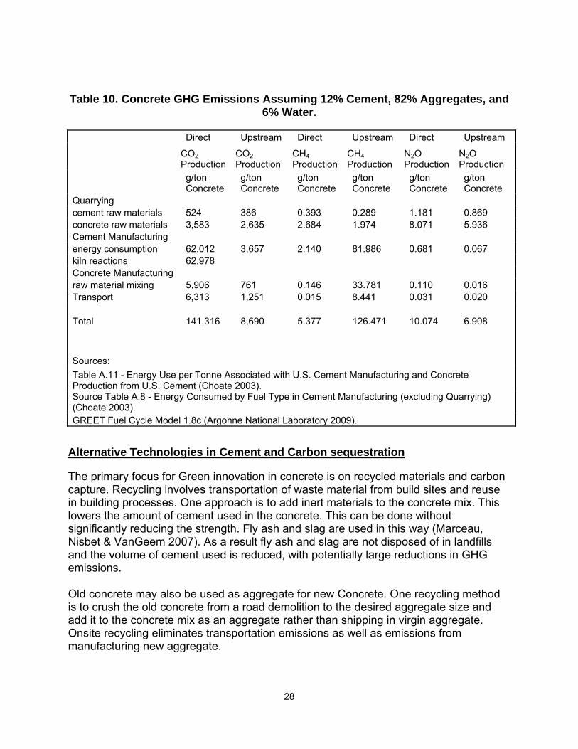
28
Table 10. Concrete GHG Emissions Assuming 12% Cement, 82% Aggregates, and 6% Water.
Direct Upstream Direct Upstream Direct Upstream
CO2 Production
CO2 Production
CH4 Production
CH4 Production
N2O Production
N2O Production
g/ton Concrete
g/ton Concrete
g/ton Concrete
g/ton Concrete
g/ton Concrete
g/ton Concrete
Quarrying cement raw materials 524 386 0.393 0.289 1.181 0.869 concrete raw materials 3,583 2,635 2.684 1.974 8.071 5.936 Cement Manufacturing energy consumption 62,012 3,657 2.140 81.986 0.681 0.067 kiln reactions 62,978 Concrete Manufacturing raw material mixing 5,906 761 0.146 33.781 0.110 0.016 Transport 6,313 1,251 0.015 8.441 0.031 0.020 Total 141,316 8,690 5.377 126.471 10.074 6.908
Sources: Table A.11 - Energy Use per Tonne Associated with U.S. Cement Manufacturing and Concrete Production from U.S. Cement (Choate 2003). Source Table A.8 - Energy Consumed by Fuel Type in Cement Manufacturing (excluding Quarrying) (Choate 2003). GREET Fuel Cycle Model 1.8c (Argonne National Laboratory 2009).
Alternative Technologies in Cement and Carbon sequestration
The primary focus for Green innovation in concrete is on recycled materials and carbon capture. Recycling involves transportation of waste material from build sites and reuse in building processes. One approach is to add inert materials to the concrete mix. This lowers the amount of cement used in the concrete. This can be done without significantly reducing the strength. Fly ash and slag are used in this way (Marceau, Nisbet & VanGeem 2007). As a result fly ash and slag are not disposed of in landfills and the volume of cement used is reduced, with potentially large reductions in GHG emissions. Old concrete may also be used as aggregate for new Concrete. One recycling method is to crush the old concrete from a road demolition to the desired aggregate size and add it to the concrete mix as an aggregate rather than shipping in virgin aggregate. Onsite recycling eliminates transportation emissions as well as emissions from manufacturing new aggregate.
29
Finished concrete is known to absorb CO2 (PCA 2009). When mixed with water and aggregate cement, it becomes reactive with air. Cement reacts with CO2 in the air with lime to form limestone through carbonation. Ca(OH)2 + CO2 = CaCO3 + H2O To the extent that the cement has carbonized, the use of concrete as aggregate is a carbon sink. Noncarbonated cement is more reactive and makes for a weaker aggregate than waste concrete that is already carbonated. Carbonation is limited by the tendency to carbonate along a thin edge of a concrete structure. A barrier forms that prevents CO2 from penetrating further and reacting with the concrete. The carbon sink effect of concrete recycling could be optimized by crushing the material, exposing its surface and stockpiling it until the carbonation process is optimized (Stolaroff, Lowry & Keith 2005). By one estimate as much as half of the CO2 emitted during the chemical process of its initial manufacture may be recovered in this way (PCA 2009). Variability is such that we will not attempt to quantify this effect in the model, but will leave this for future consideration. Recycled cement kiln dust may be used as a sink for SO2, NOX, and VOCs. It may also be used as a feedstock for potassium fertilizer production with recovery of initial investment in 3.1 years (Tureen 2003). Any use of recycled materials as feedstock would displace the carbon emissions from normal production of that feedstock from other uses. Given the current state of knowledge on the GHG emissions reductions from these newer technologies, we do not include them in GASCAP. Iron and Steel
Steel is highly purified and alloyed iron. Iron because of its reactivity exists mostly as iron oxides in its natural state and the process of refining iron into steel involves removal of oxygen and other impurities from iron ore with coke. Coke is an energy intensive purified form of coal that has had its volatile components burned away with other impurities. Iron is refined in a blast furnace where iron ore, fluxes, and coke are heated in an oxygen starved environment that draws the oxygen out of the ore. Fluxes are materials such as limestone that bond with sulfur and other impurities in iron ore to form slag (AISI 2009). Both coke production and blast furnace production are energy intensive and produce large quantities of carbon, much of which is reclaimed. Transportation construction uses large amounts of steel in bridges, guardrails, signs, reinforcing bars and other minor components of the transportation system. Upstream GHG emissions from the production and working of steel should be expected to be high from the carbon intensity of production as well as from the sheer volume of steel used in capital projects. GASCAP requires the user to select items listed on NJDOT bid-sheets for materials of calculable weight. If the weight is not known, the user will be asked to enter the weight. We will be using this approach with large inputs such as structural steel.
30
Manufacturing Process
Based on the GREET Vehicle Cycle 2.7 model we break steel production into seven processes including ore extraction, pelletizing and sinter production, coke production, blast furnace, basic oxygen furnace (BOF), electric arc furnace (EAF), and forming. The blast furnace process produces pig iron. The BOF and EAF processes purify pig iron into steel. Sheet production and rolling and stamping (Argonne National Laboratory 2007) and casting (Andersen, Hyman 2001) are the processes by which steel products are formed. The primary material inputs of finished steel are coal, iron ore, limestone, natural gas, and scrap iron and steel. Ore Extraction
Iron is very reactive and exists mostly as iron oxides in its natural state (BCS 2002b). The most common of these is hematite (Fe2O3), which with magnetite (Fe3O4) make up taconite. Taconite is a low grade ore that contains 25% - 30% iron. The iron in taconite must be purified before it is suitable for forging in a blast furnace. This is accomplished by a variety of methods, primarily by crushing the ore and removing the high grade components with magnets. Iron ores are extracted using either open pit or shaft mining methods. Drilling, blasting, loading, and transportation to the blast furnace account for 91% of the energy requirements for ore extraction. Transportation alone accounts for 75% of the energy requirements (BCS 2002b). The GREET Vehicle Model 2.7 estimates the mass of ore required to produce steel based on taconite ore (Argonne National Laboratory 2007). Pellet and Sinter Production
Agglomeration is a process by which iron ores are concentrated by sintering and pelletizing. Sintering involves insertion of a combination of iron ore, coke oven gas, limestone and others into an oven at high temperatures (2000 – 2700oF) (EPA 2010a, BCS 2002b). The mixture melts agglomerates into clumps that are crushed, much like clinker. Sinter is a flux-rich source of additional iron used in the blast furnace recovered from the waste products of primary iron production. The collection process for sintering material also keeps these dusts out of the water and air which would have been a source of pollution and environmental harm for workers in older iron production methods (EPA 2010a). Roughly 2.5 tons of raw material including water and fuel are required to produce 1 ton of sinter (EPA 2010a). Pelletizing involves heating crushed sinter or iron ore in a drum which causes the material to agglomerate into pellets of about half an inch (BCS 2002b). Coal dust may be added to improve fuel content. Coke Production
Coke is used as fuel and as an oxygen sink to produce iron in blast furnaces. The coking process is described in AP-42 (EPA 2010a). Coke is produced by crushing low sulfur low ash coal and burning off the volatile components. Coal powder may be mixed with water and oil to control density. The mixture is fed into an air tight oven to allow the
31
coal mixture to be heated in an oxygen-free environment without burning the coal. The heating requirement is roughly 15 to 18 hours at 1,650oF to 1100 oF. Upon removal the coke is quenched with water to prevent it from catching fire. It is crushed into pieces suitable for iron production in the blast furnace. Coke oven gases (COG) account for 20% - 30% of the mass of the coal. These are collected through duct systems for use as fuel in other processes such as sintering. COG is desirable as fuel because of its high VOC and CO content (EPA 2010a). Iron Production
The blast furnace provides an oxygen starved environment where iron oxides are reduced to iron by the oxidation of carbon (AISI 2009). Iron bearing material, whether ore or recovered (i.e., from recycled sources), is heated to a high temperature in the presence of a flux, using coke as the fuel (EPA 2010a). Blast furnace temperatures must exceed 1600oF to reduce the ore from oxides and sulfides, a minor component (AISI 2009). The reaction forms molten reduced iron, i.e. pig iron, CO, and slag. Blast furnace gas (BFG), like COG is recovered but is of lower value as fuel because of high CO content. Steel Production (Basic Oxygen Furnace)
The Basic Oxygen Furnace (BOF) production method uses 24% scrap steel and 76% virgin iron (Andersen, Hyman 2001). This process reduces the carbon content of pig iron and scrap in a high oxygen environment (EPA 2010a). In the presence of oxygen carbon and other impurities are oxidized with some of the iron. The heat from oxidation is sufficient to melt iron with little added fuel. The primary gaseous byproduct is CO, which is generally vented to a gas cleaning device (EPA 2010a). Steel Production (Electric Arc Furnace)
Nearly all of the raw material (98%) used in the Electric Arc Furnace (EAF) method is scrap steel (Andersen, Hyman 2001). EAFs produce carbon and alloy steels (EPA 2010a). Scrap, flux and alloy material are introduced to an EAF on a batch basis. The mixture is heated by current running through a carbon electrode. Slag and steel are poured off separately. The electrodes are gradually consumed in this process making them a source of carbon emissions (EPA 2010a). Forming
Steel may be formed in three ways: casting, rolling and stamping. All steel is cast, whether into ingots including specialized forms, or as continuous casts (Argonne National Laboratory 2007, Andersen, Hyman 2001). Steel cast into its final shape produces no further GHG emissions. GHG emission factors are estimated for rolled and stamped steel products (Argonne National Laboratory 2007). Galvanizing is a finishing procedure that we have not addressed. GHG Emissions

32
Our approach to modeling GHG emissions for steel is taken directly from the GREET Vehicle Cycle model 2.7 (Argonne National Laboratory 2007). For each step in the steel making process GHG emission factors are estimated in grams of GHG per ton of intermediate material, with conversion factors that specify the mass of each material needed to produce one ton of finished steel. We convert the emission factors to grams of GHG per ton of steel. Our conversions are shown in , which presents GHG emission factors for cast, rolled and stamped finished steel products and shows the contribution that each process makes to GHG emissions from a ton of steel. For the development GASCAP we will provide estimates of the weight of standard steel products from NJDOT’s bidsheets. This may not be possible with larger structural pieces. In that case the user will be required to enter the weight of the item.
Table 11. GREET Vehicle Cycle Model Emission Factors for Steel.
Process Emission Factors per TonSteel
(1) (2) (3) (4) (5) (6) (7) (8)
Ore Recovery
Ore Pelletizing
& Sintering
Coke Production
Blast Furnace Basic O2 Furnace
Electric ArcFurnace
Sheet Production
& Rolling
Stamping
g/ton steel g/ton steel g/ton steel g/ton steel g/ton steel g/ton steel g/ton steel g/ton steelCO2 25,957 276,673 148,069 1,363,165 1,570,966 85,315 718,637 522,460 CH4 29.47 551.49 390.45 686.36 396.08 217.77 1,730.67 1,179.46
N2O 0.63 3.80 3.05 0.62 1.01 1.14 11.78 8.33 Finished Product Emissions per Ton Steel Finished Product Emissions per lb Steel
∑ (1-6) ∑ (1-7) ∑ (1-8) ∑ (1-6) ∑ (1-7) ∑ (1-8)
Cast SteelRolled Steel Stamped
SteelCast Steel Rolled
SteelStamped
Steel
g/ton steel g/ton steel g/ton steel g/lb steel g/lb steel g/lb steel CO2 3,470,145 4,188,781 4,711,241 CO2 1,735 2,094 2,356
CH4 2,271.62 4,002.29 5,181.75 CH4 1.14 2.00 2.59
N2O 10.25 22.03 22.03 N2O 0.01 0.01 0.01
Source: GREET Vehicle Cycle Model 2.7 (Argonne National Laboratory 2007).
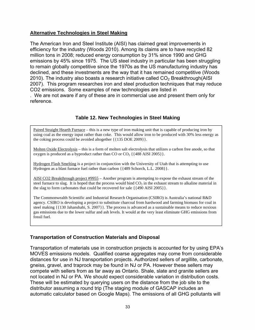
33
Alternative Technologies in Steel Making
The American Iron and Steel Institute (AISI) has claimed great improvements in efficiency for the industry (Woods 2010). Among its claims are to have recycled 82 million tons in 2008; reduced energy consumption by 31% since 1990 and GHG emissions by 45% since 1975. The US steel industry in particular has been struggling to remain globally competitive since the 1970s as the US manufacturing industry has declined, and these investments are the way that it has remained competitive (Woods 2010). The industry also boasts a research initiative called CO2 Breakthrough(AISI 2007). This program researches iron and steel production techniques that may reduce CO2 emissions. Some examples of new technologies are listed in . We are not aware if any of these are in commercial use and present them only for reference.
Table 12. New Technologies in Steel Making
Transportation of Construction Materials and Disposal
Transportation of materials use in construction projects is accounted for by using EPA’s MOVES emissions models. Qualified coarse aggregates may come from considerable distances for use in NJ transportation projects. Authorized sellers of argillite, carbonate, gneiss, gravel, and traprock may be found in NJ or PA. However these sellers may compete with sellers from as far away as Ontario. Shale, slate and granite sellers are not located in NJ or PA. We should expect considerable variation in distribution costs. These will be estimated by querying users on the distance from the job site to the distributor assuming a round trip (The staging module of GASCAP includes an automatic calculator based on Google Maps). The emissions of all GHG pollutants will
Paired Straight Hearth Furnace – this is a new type of iron making unit that is capable of producing iron by using coal as the energy input rather than coke. This would allow iron to be produced with 30% less energy as the coking process could be avoided altogether {{135 DOE 2009}}.
Molten Oxide Electrolysis – this is a form of molten salt electrolysis that utilizes a carbon free anode, so that oxygen is produced as a byproduct rather than CO or CO2 {{488 AISI 2005}}.
Hydrogen Flash Smelting is a project in conjunction with the University of Utah that is attempting to use Hydrogen as a blast furnace fuel rather than carbon {{489 Schorch, L.L. 2008}}.
AISI CO2 Breakthrough project #9955 – Another program is attempting to expose the exhaust stream of the steel furnace to slag. It is hoped that the process would bind CO2 in the exhaust stream to alkaline material in the slag to form carbonates that could be recovered for sale {{490 AISI 2005}}.
The Commonwealth Scientific and Industrial Research Organisation (CSIRO) is Australia’s national R&D agency. CSIRO is developing a project to substitute charcoal from hardwood and farming biomass for coal in steel making {{130 Jahanshahi, S. 2007}}. The process is advanced as a sustainable means to reduce noxious gas emissions due to the lower sulfur and ash levels. It would at the very least eliminate GHG emissions from fossil fuel.

34
be based on assuming the MOVES model. Emissions factors for different vehicle and equipment types used in construction projects are discussed in the next section of this report. We account for disposal of road debris based on the GHG emissions associated with transporting debris to a landfill or recycling facility. The PaLATE model (Horvath et al. 2007) assumes that emissions associated with recycled paving materials result from transportation of those materials to or from the job site. Recycled asphalt pavement (RAP) and reclaimed concrete material (RCM) are treated as byproducts of road demolition. GHG emissions connected with them are captured in the equipment used to conduct the demolition and remove these materials. Recycled materials may be sent to a landfill where unlike municipal solid waste they do not produce GHG emissions (EPA 2010a), except as they are handled by heavy equipment. Recycled materials are used as aggregate for asphalt and concrete (Horvath et al. 2007). They provide energy savings by reducing the amount and hence the GHG emissions from the extraction and processing of virgin aggregate. Other materials modeled in PaLATE including baghouse fines, flyash, ground glass, kiln dust, blast furnace slag, and others are byproducts of other industrial processes and are treated in the same way as RAP and RCM. Aside from recycling in place, reasonable estimates of distances from jobsites to landfills, recycling facilities and distributors of virgin aggregates and substitutes will be needed. Other Materials
We have addressed the material requirements of the core issues of pavement. We have covered the inputs of asphalt and reinforced concrete, and many of the treatments used to maintain and repair these. The PaLATE Model (Horvath et al. 2007) allows use of the same materials used for the base and pavement layers in the subbase, with the exception of soil. Fill of various kinds and topsoil are assumed to have no process GHG emissions associated except for extraction and transport. The extraction component is an equipment input. Transport will be calculated as per ton per mile from a heavy truck using EPA’s MOVES model. Pedestrian facilities include sidewalks and possibly trails. The principal materials used for these are concrete and asphalt. Gravel can be accounted for as it is similar to aggregate. For the most part we have addressed bridges, dams, culverts, tunnels and related structures. From a volumetric perspective we have addressed the materials that make up the bulk of these structures. However, we have not included minor inputs such as paint, plastics, epoxy, galvanizing of steel. Error! Reference source not found. shows emission factors for rubber and three varieties of plastics and a default. Emission factors for zinc are presented. Zinc is primarily used for galvanizing in the GREET 2.7 Vehicle Cycle model (Argonne National Laboratory 2007). The zinc emission factors should be applicable to galvanizing of steel used in transportation capital projects. The Vehicle Cycle model includes a number of other metals. Emission factors for virgin and recycled aluminum are also shown in Error! Reference source not found..
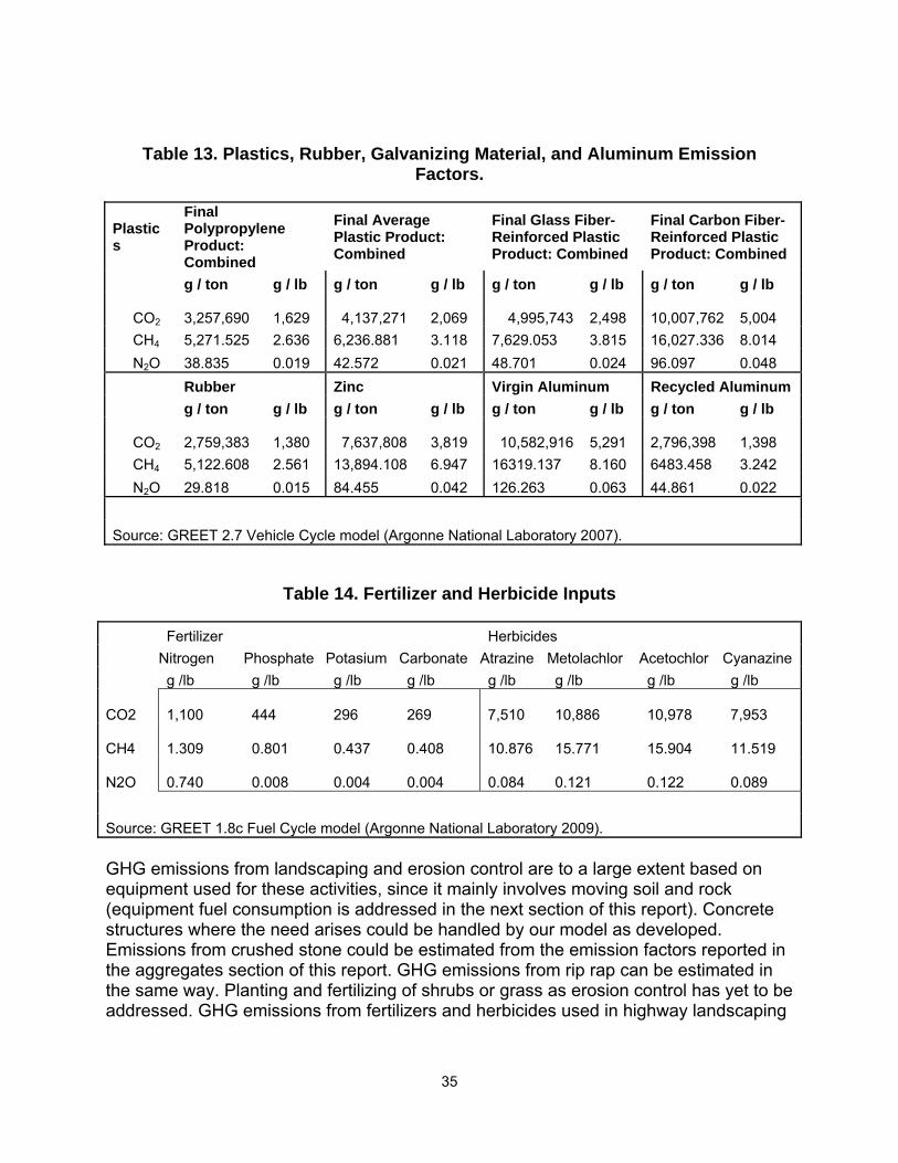
35
Table 13. Plastics, Rubber, Galvanizing Material, and Aluminum Emission Factors.
Plastics
Final Polypropylene Product: Combined
Final Average Plastic Product: Combined
Final Glass Fiber-Reinforced Plastic Product: Combined
Final Carbon Fiber-Reinforced Plastic Product: Combined
g / ton g / lb g / ton g / lb g / ton g / lb g / ton g / lb
CO2 3,257,690
1,629 4,137,271
2,069 4,995,743
2,498
10,007,762
5,004
CH4 5,271.525 2.636 6,236.881 3.118 7,629.053 3.815 16,027.336 8.014 N2O 38.835 0.019 42.572 0.021 48.701 0.024 96.097 0.048 Rubber Zinc Virgin Aluminum Recycled Aluminum g / ton g / lb g / ton g / lb g / ton g / lb g / ton g / lb
CO2 2,759,383
1,380 7,637,808
3,819 10,582,916
5,291
2,796,398
1,398
CH4 5,122.608 2.561 13,894.108 6.947 16319.137 8.160 6483.458 3.242 N2O 29.818 0.015 84.455 0.042 126.263 0.063 44.861 0.022 Source: GREET 2.7 Vehicle Cycle model (Argonne National Laboratory 2007).
Table 14. Fertilizer and Herbicide Inputs
Fertilizer Herbicides Nitrogen Phosphate Potasium Carbonate Atrazine Metolachlor Acetochlor Cyanazine g /lb g /lb g /lb g /lb g /lb g /lb g /lb g /lb CO2 1,100 444 296 269 7,510 10,886 10,978 7,953 CH4 1.309 0.801 0.437 0.408 10.876 15.771 15.904 11.519 N2O 0.740 0.008 0.004 0.004 0.084 0.121 0.122 0.089 Source: GREET 1.8c Fuel Cycle model (Argonne National Laboratory 2009). GHG emissions from landscaping and erosion control are to a large extent based on equipment used for these activities, since it mainly involves moving soil and rock (equipment fuel consumption is addressed in the next section of this report). Concrete structures where the need arises could be handled by our model as developed. Emissions from crushed stone could be estimated from the emission factors reported in the aggregates section of this report. GHG emissions from rip rap can be estimated in the same way. Planting and fertilizing of shrubs or grass as erosion control has yet to be addressed. GHG emissions from fertilizers and herbicides used in highway landscaping
36
are shown in Error! Reference source not found. from the GREET 1.8c Fuel Cycle model(Argonne National Laboratory 2009).
REVIEW OF LIFE-CYCLE CONSTRUCTION EQUIPMENT EMISSIONS
This section addresses assumptions to be made for the modeling of greenhouse gas (GHG) emissions from construction equipment in GASCAP. The model will account for lifecycle emissions from construction equipment, materials, and maintenance practices for transportation facilities in New Jersey. The principal focus of this section is on the lifecycle emissions associated with fuels consumed by construction equipment during operations for construction, rehabilitation, and maintenance of transportation facilities. We cover both existing equipment but with an additional focus on technological improvements and increased use of biofuels. The model used addresses direct and upstream emissions from fuel consumption in construction equipment. Direct emissions are GHG emissions that result from fuel combustion in construction equipment under the control of contractors or the New Jersey Department of Transportation. Upstream emissions are GHG emissions that result from the extraction, transportation, refining, and distribution of fuels used in construction projects. The Argonne National Laboratory GREET 1.8c Fuel Cycle Model (Argonne National Laboratory 2009) is used to estimate upstream emissions for fuels used in construction equipment. The GREET model estimates CO2, CH4, and N2O emissions and was designed to estimate upstream and direct emissions for on-road vehicles. The EPA Office of Transportation and Air Quality NONROAD model was designed to estimate criteria pollutants in off-road equipment (EPA 2008a). (EPA 2008a)(EPA 2008a) NONROAD was accessed by writing scripts for the National Mobile Inventory Model (NMIM) application. NMIM provides access to the MOBILE and NONROAD models. Although NMIM uses the 2008 version of NONROAD, it is documented here based on NONROAD 2005.4 Carbon dioxide (CO2) emissions are estimated from brake-specific fuel consumption (BSFC) on the assumption that nearly all of the carbon in fuel is oxidized to CO2 either in the engine or in the atmosphere. Methane (CH4) and nitrous oxide (N2O) are modeled by manipulation of the NONROAD model and by adapting emission factors from the GREET model, respectively. Black carbon particulate matter was estimated by applying a speciation factor from the literature. We note the following limitations with the NONROAD model:
• CO2 as modeled in the GREET model includes oxidized fugitive and partially burned hydrocarbons and carbon monoxide (CO), whereas NONROAD only
4, The NONROAD 2008 documentation was not published on the EPA website until August 2010 and does not differ substantially with respect to our assumptions about construction equipment. The changes in NONROAD 2008 primarily concern emission reductions for recreational equipment following incorporation of EPA standards in 2008 and changes in evaporative emissions as a result of use of ethanol as an additive to gasoline. Since the Carbon Footprint model uses NMIM’s unadjusted NONROAD 2008 evaporative emission estimations our results are unaffected. (EPA 2009a)(EPA 2009a)
37
includes the latter. We account for oxidization of hydrocarbons emitted as volatile fugitive and partially burned fuel based on carbon content.
• Methane (CH4) emissions are not directly modeled although it is possible to estimate hydrocarbon emissions with or without CH4, which allows estimation of CH4 as a residual.
• Nitrous oxide (N2O) is not modeled. • Black carbon or elemental carbon particulate matter is not estimated.
The balance of this section is a discussion of how GASCAP accounts for the global warming potential (GWP) of GHGs and black carbon. After discussing GHGs, black carbon, and the relevant accounting principles, we briefly address the chemistry of fuel consumption. We establish a basis with which to account for direct emissions that occur as a result of equipment inputs using standard fossil fuels. The NONROAD 2008 model through NMIM is used to address emissions of GHGs and criteria pollutants from standard fossil fuels including diesel oil (EPA 2004a)(EPA 2004a)(EPA 2004a) and gasoline as petroleum-based products and compressed natural gas (CNG) and liquefied petroleum gas (LPG) (EPA 2005b), which may be produced from either petroleum or natural gas. We discuss alternatives to petroleum and natural gas-based fuels including biomass and coal-based alternatives using the GREET model (Argonne National Laboratory 2009). Since the GREET model is a full lifecycle model it allows us to present upstream, direct, and combined emissions for all variants of the four fuel types modeled in NONROAD. Because NONROAD does not model the alternative fuels covered in the GREET model, we recognize that there is uncertainty in the performance and direct emissions of alternative fuels in existing non-road construction equipment. The GREET model treats direct emissions of alternative fuels as identical to those of standard fuels. NONROAD – Direct Emissions
The NONROAD model is based on EPA regulation of criteria pollutants for off-road spark ignition (typically using gasoline, but also alternative fuels) and compression ignition engines (which use diesel fuel). These regulations were developed and phased in during the 1990s and the first decade of the 21st century (EPA 2004a, EPA 2005b). The phasing in of these regulations introduces an element of temporal variation because it is presumed in NONROAD that new equipment met the existing standards for the year in which it was manufactured. Criteria pollutants include hydrocarbons (HC), carbon monoxide (CO), oxides of nitrogen excluding nitrous oxide (NOX), sulfur dioxide (SO2), and particulate matter both smaller than 2.5 microns (PM2.5) and smaller than 10 microns in diameter (PM10). The last two categories overlap. BSFC is covered and is the basis of CO2, and SO2 emissions and a correction to the particulate matter based on sulfur content of diesel(EPA 2004a, EPA 2005b). Spark Ignition Emission Standards Implementation
Spark ignition engines use gasoline, CNG, and LPG as fuel. They are classified by size as large and small with a dividing line of 25 hp(EPA 2005b). Both engine types are sub-
38
classified. Small engines have five designations by Roman numeral (I-V). All small spark ignition engines are gasoline powered. Classes I and II are non-handheld machines. Class I is smaller than 225 cc and Class II is larger. Class I engines have power ratings between 3 and 6 hp. Power ratings for Class II are from 6 to 25 hp. Classes III through V are handheld. Class III is smaller than 20cc with a power range 0-1 hp. Class IV is between 20cc and 50cc with a power range of 1-3 hp. Class V includes handheld devices with engines larger than 50cc and a power range 3-6 hp. NONROAD does not adjust for transient adjustment factors5 in spark-ignition engines smaller than 25 hp(EPA 2005b). Phase 1 regulation for large spark ignition engines took effect in 2004 and were replaced by Phase 2 regulations in 2007 for gasoline engines larger than 25 hp and all CNG and LPG engines which are all larger than 25 hp. Phase 1 emission standards for smaller gasoline engines with power ratings less than or equal to 25 hp began in 1996 and was completed in 1997 (EPA 2005b). Phase 2 implementation for smaller gasoline engines was incremental and varied by engine class. Non-handheld gasoline machines include two-stroke and four-stroke gasoline engines with power ratings from 0 to 6 hp (Class I) and from 6 to 25 hp (Class II) (EPA 2005b)(EPA 2005b)(EPA 2005b). Phase 2 emission standards implementation for the larger Class II engines was begun in 2001 and completed in 2005. Implementation of Phase 2 standards for Class I engines began in 2007 and was completed in 2008. Handheld gasoline engines are all small two-stroke engines (EPA 2005b). Phase 2 emission standards for Class III engines rated 1 hp or less and Class IV engines rated from 1 to 3 were implemented between 2002 and 2005. In 2002 25% of the population of Class III and Class IV equipment was on the new standard in the first year. The Phase 2 share increased in 25% increments until the Phase 1 standard was replaced in 2005. Phase 2 standards for larger Class V handheld equipment rated between 3 and 6 hp were not implemented until 2004 – 2007, but using the same incremental approach used with Classes III and IV and the smaller non-handheld engines in Class I. Compression Ignition Emission Standards Implementation
Larger diesel engines with power ratings from 175 to 750 hp were the first compression ignition engines to have full regulation of criteria pollutants (EPA 2004a). Tier 1 regulations established emission standards for HC, NOX, CO, and PM emissions in 1996. Tier 2 regulations tightened and consolidated the emission standards for HC and NOX into a combined standard for NMHC and NOX. Emission standards for CO and PM were tightened as well. Tier 2 regulations took effect between 2001 and 2003. In 2006 Tier 3 tightened the emission standard for NMHC and NOX. Table 15 shows federal emission standards modeled in NONROAD for compression ignition or diesel engines (EPA 2004a). 5 NONROAD uses transient adjustment factors to compensate for the variability of engine load. NONROAD estimates are taken from laboratory results without the variability of load that occurs under normal real world use (EPA 2004a, EPA 2005b)

39
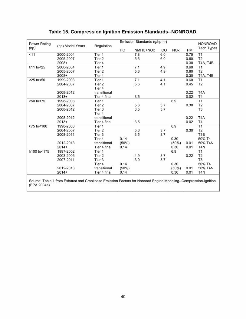
40
Table 15. Compression Ignition Emission Standards--NONROAD.
Power Rating (hp) (hp) Model Years Regulation
Emission Standards (g/hp-hr) NONROAD Tech Types HC
NMHC+NOx CO NOx PM
<11 2000-2004 Tier 1 7.8 6.0 0.75 T1 2005-2007 Tier 2 5.6 6.0 0.60 T2 2008+ Tier 4 0.30 T4A, T4B ≥11 to<25 2000-2004 Tier 1 7.1 4.9 0.60 T1 2005-2007 Tier 2 5.6 4.9 0.60 T2 2008+ Tier 4 0.30 T4A, T4B ≥25 to<50 1999-2003 Tier 1 7.1 4.1 0.60 T1 2004-2007 Tier 2 5.6 4.1 0.45 T2
2008-2012 Tier 4 transitional 0.22 T4A
2013+ Tier 4 final 3.5 0.02 T4 ≥50 to<75 1998-2003 Tier 1 6.9 T1 2004-2007 Tier 2 5.6 3.7 0.30 T2 2008-2012 Tier 3 3.5 3.7 T3
2008-2012 Tier 4 transitional 0.22 T4A
2013+ Tier 4 final 3.5 0.02 T4 ≥75 to<100 1998-2003 Tier 1 6.9 T1 2004-2007 Tier 2 5.6 3.7 0.30 T2 2008-2011 Tier 3 3.5 3.7 T3B
2012-2013 Tier 4 transitional
0.14 (50%)
0.30 (50%) 0.01
50% T4 50% T4N
2014+ Tier 4 final 0.14 0.30 0.01 T4N ≥100 to<175 1997-2002 Tier 1 6.9 T1 2003-2006 Tier 2 4.9 3.7 0.22 T2 2007-2011 Tier 3 3.0 3.7 T3
2012-2013 Tier 4 transitional
0.14 (50%)
0.30 (50%) 0.01
50% T4 50% T4N
2014+ Tier 4 final 0.14 0.30 0.01 T4N Source: Table 1 from Exhaust and Crankcase Emission Factors for Nonroad Engine Modeling--Compression-Ignition (EPA 2004a).
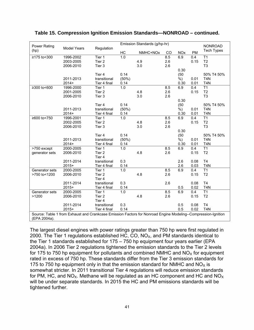
41
Table 15. Compression Ignition Emission Standards—NONROAD – continued. Power Rating (hp) Model Years Regulation
Emission Standards (g/hp-hr) NONROAD Tech Types HC NMHC+NOx CO
NOx PM
≥175 to<300 1996-2002 Tier 1 1.0 8.5 6.9 0.4 T1 2003-2005 Tier 2 4.9 2.6 0.15 T2 2006-2010 Tier 3 3.0 2.6 T3
2011-2013 Tier 4 transitional
0.14 (50%)
0.30 (50%) 0.01
50% T4 50% T4N
2014+ Tier 4 final 0.14 0.30 0.01 T4N ≥300 to<600 1996-2000 Tier 1 1.0 8.5 6.9 0.4 T1 2001-2005 Tier 2 4.8 2.6 0.15 T2 2006-2010 Tier 3 3.0 2.6 T3
2011-2013 Tier 4 transitional
0.14 (50%)
0.30 (50%) 0.01
50% T4 50% T4N
2014+ Tier 4 final 0.14 0.30 0.01 T4N ≥600 to<750 1996-2001 Tier 1 1.0 8.5 6.9 0.4 T1 2002-2005 Tier 2 4.8 2.6 0.15 T2 2006-2010 Tier 3 3.0 2.6 T3
2011-2013 Tier 4 transitional
0.14 (50%)
0.30 (50%) 0.01
50% T4 50% T4N
2014+ Tier 4 final 0.14 0.30 0.01 T4N >750 except 2000-2005 Tier 1 1.0 8.5 6.9 0.4 T1 generator sets 2006-2010 Tier 2 4.8 2.6 0.15 T2
2011-2014 Tier 4 transitional 0.3 2.6 0.08 T4
2015+ Tier 4 final 0.14 2.6 0.03 T4N Generator sets 2000-2005 Tier 1 1.0 8.5 6.9 0.4 T1 >750 to<1200 2006-2010 Tier 2 4.8 2.6 0.15 T2
2011-2014 Tier 4 transitional 0.3 2.6 0.08 T4
2015+ Tier 4 final 0.14 0.5 0.02 T4N Generator sets 2000-2005 Tier 1 1.0 8.5 6.9 0.4 T1 >1200 2006-2010 Tier 2 4.8 2.6 0.15 T2
2011-2014 Tier 4 transitional 0.3 0.5 0.08 T4
2015+ Tier 4 final 0.14 0.5 0.02 T4N Source: Table 1 from Exhaust and Crankcase Emission Factors for Nonroad Engine Modeling--Compression-Ignition (EPA 2004a).
The largest diesel engines with power ratings greater than 750 hp were first regulated in 2000. The Tier 1 regulations established HC, CO, NOX, and PM standards identical to the Tier 1 standards established for 175 – 750 hp equipment four years earlier (EPA 2004a). In 2006 Tier 2 regulations tightened the emission standards to the Tier 2 levels for 175 to 750 hp equipment for pollutants and combined NMHC and NOX for equipment rated in excess of 750 hp. These standards differ from the Tier 3 emission standards for 175 to 750 hp equipment only in that the emission standard for NMHC and NOX is somewhat stricter. In 2011 transitional Tier 4 regulations will reduce emission standards for PM, HC, and NOX. Methane will be regulated as an HC component and HC and NOX will be under separate standards. In 2015 the HC and PM emissions standards will be tightened further.
42
For diesel engines between 50 hp and 175 hp Tier 1 regulations begin earlier (1997-8) than Tier 1 regulations for smaller diesel engines but only address NOX emissions (EPA 2004a). It is only with the implementation of Tier 2 in 2003-4 that emissions standards for combined NMHC and NOX, CO, and PM are established, although the emissions standards are comparable with other Tier 2 standards. With Tier 3 regulations emissions standards for NMHC and NOX were tightened in 2007-8. Tier 4 regulations will tighten emission standards for PM and establish separate significantly more stringent emission standards for HC and NOX for engines between 75 and 175 hp to be phased in from 2012-14. For smaller diesel engines (<50 hp) Tier 1 regulations introduced standards for combined non-methane hydrocarbons (NMHC) and NOX, CO, and PM (EPA 2004a). Tier 2 regulations tightened emission standards for PM from engines between 25 and 50 hp and NMHC and NOX from all engines smaller than 50 HP. Tier 4 halved permissible PM levels from Tier 2 levels. This anticipates drastic reductions in sulfur content for diesel fuel. Tier 1 emission standards for diesel engines between 25 and 50 hp were implemented in 1999 and replaced with Tier 2 standards in 2004. Tier 4 emission standards were implemented in 2008. A more stringent PM standard will be implemented in 2013. Emission standards for smaller diesel engines less than 11 hp and between 11 and 25 hp were implemented at the same time. For engines rated less than 25 hp Tier 1 emission standards were implemented in 2000 and replaced by Tier 2 standards in 2005. Tier 4 emission standards were implemented for smaller engines in 2008. Modeling Approach
The engines modeled in GREET are on the large end of what is modeled in NONROAD non(EPA 2004a, EPA 2005b), and do not contain the detailed disaggregation by vehicle type, vintage, and power rating. The impact of this assumption is minor because we know BSFC from NONROAD, are using the GREET model for upstream emissions only, and The GREET model treats direct emissions from analogous fuels produced from multiple pathways as equal (Argonne National Laboratory 2009). We model direct emissions from non-road engines using NONROAD for the relevant fuels: diesel, gasoline, CNG and LPG. We then model upstream emissions from these fuels using the GREET model for each of the fuels from each fuel pathway. The GREET model treats direct emissions from fuels produced from different pathways as equal. We are justified for this reason in modeling direct emissions as standard fuels. We summarize the models used as sources for data in

43
.

44
Table 16. Models Used to Estimate GHG Emissions
CO2 CH4 N2O BC Upstream Emissions1 GREET7 GREET7 GREET7 EPA model6 Direct Emissions
Exhaust Emissions1 NONROAD3 NONROAD4 GREET5 EPA model6 Evaporative Emissions2
NONROAD7 NONROAD7 N/A N/A
1. Upstream and exhaust emissions are for diesel, gasoline, CNG, and LPG. 2. Evaporative emissions are for gasoline only. 3. CO2 emissions are taken from NONROAD except that the carbon from NMOG is
adjusted stoichiometrically and added to the NONROAD estimate. 4. CH4 is estimated as a residual of TOG and NMOG. 5. N2O is estimated as a constant 0.006 g/hp-hr per GREET. 6. BC is estimated as the product of NONROAD PM2.5 and fuel specific black carbon
speciation factors for diesel and gasoline and a generic speciation factor for CNG and LPG (Battye, Boyer & Pace 2002).
7. Uncorrected emissions are used. NONROAD and MOBILE were designed primarily to model criteria pollutants including organic compounds of various designations. Particulate matter is composed of sulfates, nitrate and organic and elemental carbon (Liu et al. 2005)(Liu et al. 2005)(Liu et al. 2005). CO2 emissions are calculated as a residual from the carbon content of the fuel after VOCs are accounted for. It is therefore presumed correctly that most of the CO is converted into CO2 or behaves as CO2 in the atmosphere (Wayne 1991). CH4 may be calculated as a residual, i.e. the difference between total organic gases (TOG) and non-methane organic gases (NMOG). N2O cannot be estimated directly or indirectly through NONROAD. It is possible to estimate the sulfate and carbon fractions of particulate matter, but it is not possible to distinguish between elemental and organic carbon in the particulate matter. The Motor Vehicle Emission Simulator (MOVES) model distinguishes between elemental and organic carbon particulate matter, but does not yet have a released off-road component (EPA 2010d)(EPA 2010d)(EPA 2010d). Construction equipment emissions include those associated with combustion of fuel and losses of fuel to evaporation. The California Department of Transportation (CalTrans) in conjunction with the University of California at Davis developed a spreadsheet tool to estimate for PM, NOX, CO2, CO, and THC emissions from diesel retrofits and replacements between 2010 and 2015 (Wang et al. 2008)(Wang et al. 2008)(Wang et al. 2008). Their spreadsheet tool was used to estimate emissions reductions at the regional level for six equipment types6, which account for 49% of NOX emissions. Emissions were measured at the county level using OFFROAD (the California equivalent to NONROAD). Regional assumptions for population, activity level, and power rating were taken from OFFROAD. Caltrans decision to use activity data from OFFROAD was because they aggregate the data to the county level.
6 Equipment types include rollers, rubber tire loaders, graders, generator sets, scrapers, and tractor-loader-backhoes.

45
The NONROAD 2008 model (EPA 2004a, EPA 2005b) addresses construction equipment by its function, power rating, fuel consumption rate and fuel type. We are not able to estimate activity from the NONROAD model. NONROAD activity data is based on aggregated data used for inventories at the county state or national level (EPA 2004b, EPA 2005c).In order to apply NONROAD at the microscopic level scripts i.e. short macros, were used to estimate one hour of activity for each machine we modeled. Accurate activity data for New Jersey construction, rehabilitation and general maintenance should take into account factors such as climate and actual practices. The modeling approach used here is an approximation because it estimates emissions based on an average hour of use estimated from steady state laboratory measurements. However, emissions are dependent on load and idling time. Direct measurement can be done using Portable Emissions Measurement Systems (PEMS). This would allow emissions assessment under a variety of circumstances to determine differences in task, idling time, weather, and other machine specific conditions that NONROAD does not account for (Rasdorf et al. 2010)(Rasdorf et al. 2010)(Rasdorf et al. 2010). However, direct measurement is expensive and is currently an active area of research; for example, detailed activity data and an understanding of the operating modes of various construction equipment needs to be determined. One example is a large study (Rasdorf et al. 2010) that analyzed emissions for nine types of equipment7 at one power rating each. The types of equipment selected were intended to include the types with the highest emissions of criteria pollutants, but does not cover all the possible equipment that might be used on a construction project, especially as the vintage of the equipment would likely not correspond to the estimates from a single study. The study by (Rasdorf et al. 2010) outlines procedures for collecting data using PEMS, but this is clearly beyond the scope of the current project. Evaporative and Refueling Emissions
Evaporative emissions are losses of the volatile components of fuel to a gaseous state, essentially without chemical transformation of the fuel material (EPA 2005e)(EPA 2005e)(EPA 2005e). Increases in ambient or engine temperatures increase the likelihood that fuels will vaporize. Diurnal emissions refer to evaporation caused by higher ambient temperatures during daylight hours. Hot soak and running losses refer to evaporative emissions that occur as a result of a hot engine. Hot soak emissions occur after an engine has been turned off, but before it has cooled to ambient temperature. Running losses occur while a hot engine is running. Permeation losses occur when fuel has soaked through containers or hoses and become exposed to air. Diffusion losses occur when fuel is otherwise exposed to air. These include displacement losses and spillage, which refer to evaporation of fuel that occurs during refueling because of displaced vapors or when spilled fuel evaporates. Crankcase emissions and resting loss occur through the crankcase and fuel tank, respectively, when the temperature is stable. NONROAD (EPA 2005b)(EPA 2004a) assumes that evaporative emissions are only a concern for gasoline engines. It is argued that evaporative emissions are negligible for
7 Equipment covered by (Rasdorf et al. 2010) includes backhoes, bulldozers, excavators, generators, motor graders, off-highway trucks, rubber tire loaders, track loaders, and skid-steer loaders.

46
CNG and LPG engines because these are designed to contain fuel that is in a gaseous state at ambient temperatures and pressures. Diesel on the other hand contains only components that are heavy enough so as not to be volatile at ambient temperatures and pressures. Only gasoline contains components that are usually but not always liquid at ambient temperatures and pressures and therefore likely to change phase(Speight 2007). However, NONROAD accounts for hydrocarbon crankcase emissions from diesel engines (EPA 2004a). Detailed guidance for estimating evaporative and refueling emissions as done in NONROAD is available (EPA 2005e, EPA 2004c). Since we incorporate evaporative and refueling emissions unaltered from the model output, the reader is referred there. Exhaust Emissions
EPA published separate NONROAD model guidance for estimating exhaust emissions for spark ignition (EPA 2005b) and compression ignition engines (EPA 2004a). Spark ignition engines include gasoline, CNG and LPG engines. Gasoline engines may use two or four-stroke cycles. Compression ignition engines use diesel oil. Although EPA has published emissions modeling software we adjust fuel consumption to apply variations in the upstream emissions from the various fuel pathways discussed in the GREET model (Argonne National Laboratory 2009)(Argonne National Laboratory 2009)(Argonne National Laboratory 2009). We estimate emissions for CO2, CH4, N2O and black carbon particulate matter. We estimate black carbon as a fraction of particulate matter smaller than 2.5 microns. NONROAD does not differentiate between organic and elemental carbon particulate matter. We estimate direct N2O emissions with the GREET model (Argonne National Laboratory 2009). The equipment discussion addresses spark ignition and compression ignition engines separately. The discussion of spark ignition engines focuses primarily on variations among small gasoline engines (<25 hp), since large spark ignition engines vary by fuel type rather than by power rating (EPA 2005b). The first decade of the twenty-first century witnessed a sharp decrease in the sulfur content of diesel fuel from 3,000 ppm to 15 ppm . This process is complete or will be completed early in the 2010s for most fuel used in compression ignition engines of various power ratings. Much of the temporal variation in emissions from diesel fuel results from the phased implementation of new fuel sulfur restrictions. NONROAD Model Basics
The NONROAD model applies laboratory test results to approximate emissions and fuel consumption under operating conditions. The NONROAD model first estimates zero-hour steady-state criteria pollutant emissions and fuel consumption. Zero-hour emissions are not adjusted for normal deterioration of engine performance over its useful life. Steady-state refers to running an engine under a constant load under laboratory conditions without a load adjustment to correct for variations in load during normal use. NONROAD estimates deterioration factors (DF) and transient adjustment

47
factors (TAF) to correct for the zero-hour state and the steady state emissions, respectively. Emissions are estimated in grams per horsepower-hour (hp-hr). Fuel consumption is estimated in pounds per hp-hr. Zero-hour steady-state emissions are estimated for different engine types based on power rating, fuel type and function. NONROAD provides separate procedures for adjusting particulate matter emissions, gaseous emissions including hydrocarbons, CO, and NOX, and fuel consumption (EPA 2004a)(EPA 2004a)(EPA 2004a). The formulas are shown in Table 17. EFadj represents the adjusted emission factors for HC, CO, NOX, PM, and BSFC. EFss represents the steady state zero hour emission factors. SPMadj is an adjustment factor that accounts for the impact of variations in fuel sulfur levels on particulate matter levels. Since no deterioration factor is applied to BSFC the adjusted fuel consumption rate is the product of the steady-state fuel consumption rate and the TAF. Deterioration factors are estimated for HC, CO, and NOX so the adjusted emission factor for each of these is the product of the zero-hour steady-state emission rate, the TAF and the DF. The same procedure is used to estimate adjusted particulate matter emissions, however, reductions in sulfur content over the last decade reduce the volume of sulfate in particulate matter and must also be accounted for. The sulfur adjustment to particulate matter is used unchanged from the NONROAD model, which includes this adjustment. Zero-hour steady-state emissions and fuel use, transient emissions factors, and deterioration factors are reported in Appendix A Tables A1-3 for spark ignition engines and in Appendix B Tables B1-3 for compression ignition engines. Zero-Hour, Steady-State Emissions and Fuel Use.
The unadjusted tables used in NONROAD track emissions of HC, CO, NOX, PM and BSFC (EPA 2004a, EPA 2005b). Hydrocarbons are essentially unburned and partially consumed fuel. They include a multiplicity of compounds that are classified by volatility and the presence of oxygen (EPA 2005a)(EPA 2005a)(EPA 2005a). NONROAD does not address oxidation of hydrocarbons to CO2, although the GREET model addresses this phenomenon. CO is a product of partial combustion that is readily oxidized into CO2 in the atmosphere and is so modeled in NONROAD (EPA 2004a, EPA 2005b)(EPA 2004a, EPA 2005b)(EPA 2004a, EPA 2005b). The zero-hour steady-state emissions factors apply to unused equipment with zero hours of use run at a constant rate under laboratory conditions.

48
Table 17. Adjustments to Zero-Hour Steady State Rates.
Brake-Specific Fuel Consumption EFadj(BSFC) = EFss(BSFC) * TAF(BSFC) Emission Factors for HC, CO, and NOX EFadj(HC, CO, NOX) = EFss(HC, CO, NOX) * TAF(HC, CO, NOX) * DF(HC, CO, NOX) Emission Factors for Particulate Matter EFadj(PM) = EFss(PM) * TAF(PM) * DF(PM) - SPmadj Where: EFadj is the adjusted emission factor; EFss is the steady-state [zero-hour] emission factor; TAF is the transient adjustment factor; DF is the deterioration factor; and SPMadj is the sulfur adjustment to particulate matter. Sources: Exhaust and Crankcase Emission Factors for Nonroad Engine Modeling—Compression-Ignition (EPA 2004a). Exhaust Emission Factors for Nonroad Engine Modeling: Spark-Ignition (EPA 2005b). Transient Adjustment Factors
Most off-road engines operate with variable or transient loads but the emissions testing for the NONROAD model is done with steady-state tests (EPA 2004a, EPA 2005b). At variable loads engine efficiency should vary because the ratio of fuel to air varies (Stone 1992)(Stone 1992)(Stone 1992). TAFs correct for inefficiencies from this type of variability. They are generally stated as a factor of one or greater, although the manual states that they may be less than 1.0 (EPA 2004a). TAFs are multiplied by the four steady-state emission factors and the fuel consumption factor to produce transient factors (EPA 2004a). A TAF of one (1.0) indicates that load variability has no effect on emissions. This assumption is made for small spark ignition engines (<25 hp), Tier four compression ignition engines, large (>25 hp) spark ignition made under Phase 2 standards (2007-8 and later) and equipment that usually runs at a steady state, such as generators, pumps, and compressors (EPA 2004a, EPA 2005b). Deterioration Factors
Generally engines lose efficiency over their useful life. NONROAD estimates this effect for the four zero-hour emission factors but not for fuel consumption (EPA 2004a, EPA 2005b)(EPA 2004a, EPA 2005b)(EPA 2004a, EPA 2005b). Deterioration-adjusted emissions are modeled as the product of zero-hour emissions and a deterioration factor based on the proportion of the median useful life of an equipment piece expended. The deterioration factor is a function of median life expended up to but not beyond the point where half of the population has been scrapped. The NONROAD model assumes that in order to continue functioning an equipment piece must be maintained to a certain de facto standard so that it is unrealistic that equipment will continue to deteriorate if it is

49
still in service when half the population has been scrapped (EPA 2005d). The deterioration factor is expressed: DF = 1 + A * AFb (for 0.0 < AF < 1.0) where A is the maximum proportionate increase in emissions at the end of the median life of the equipment type by fuel type and power rating; AF is the proportion of the median life already expended; and b is a constant that regulates acceleration of emissions. The guidance cautions that there is little PM deterioration data and that PM deterioration estimates are based on HC deterioration data for spark ignition engines (EPA 2005d)(EPA 2005d)(EPA 2005d). If b is equal to 1, deterioration is at a constant rate. If b is less than one the engine experiences a rapid initial increase in emissions which decelerates as the end of the median life approaches. If b is greater than one, the increase in emissions is initially slow but accelerating. The exponential b constant is set to 0.5 for small 4-stroke spark ignition engines and 1.0 for small (<25hp) 4-stroke gasoline engines and 1.0 for all 2-stroke gasoline and large (>25hp) spark ignition engines (EPA 2005d). The b constant is set equal to 1.0 for all compression ignition engines. Median life is measured as hours of use at full load taken from the Power Systems Research database (EPA 2005d). These values may be converted to median life in years by dividing them by the product of average use stated in hours of use per year and average load stated as a fraction of full load (EPA 2005d). Adjustments to NONROAD GHG Definitions
Total hydrocarbon (THC) emissions include those emissions that are measureable with a flame ionization detector calibrated with propane (EPA 2005a). This definition excludes oxygenated hydrocarbons such as alcohols and aldehydes, which are similar in reactivity with ozone forming hydrocarbons in the atmosphere. Together hydrocarbons and oxygenated variants are combined into a class called total organic gases (TOG). Because CH4 is less reactive than other hydrocarbons non-methane classifications are also estimated. These are non-methane hydrocarbons (NMHC) and non-methane organic gases (NMOG), respectively. By definition VOCs are all materials included in the TOG classification, except CH4, ethane, acetone or other compounds that are rare in engine exhaust such as PFCs or HFCs (EPA 2005a). In practice only CH4 and ethane are discounted by EPA because the other compounds are present in negligible quantities. Differences among these hydrocarbon classifications are based on the mass of the components not carbon weight. Once in the atmosphere CO and hydrocarbons in the broadest sense, i.e. TOG, are ultimately transformed into CO2. CH4 is less reactive than VOCs by more than one order of magnitude (EPA 2005a). Because they survive longer in the atmosphere CH4 emissions are treated separately from VOC emissions in GHG accounting. Through photolysis CH4 oxidizes to CO (Wayne 1991). CO emissions as modeled by NONROAD (EPA 2004a, EPA 2005b) are assumed to oxidize further from CO to CO2. The GREET model (Argonne National Laboratory 2009) includes VOC emissions in CO2 estimates, although CO2 emissions produced as a direct product of combustion with CO and VOCs
50
are presented as well in the model’s output tables. NONROAD does not incorporate VOCs into CO2 emissions estimates (EPA 2004a, EPA 2005b). The approach used in the GREET model is preferred for application to the NONROAD data because it accounts for the GHG impact of carbon emissions as CO2 or CH4 more completely than the approach taken by NONROAD assuming the NONROAD definitions. It is tempting to use the NONROAD definition for VOCs (EPA 2005a) because it correctly excludes CH4. However, VOCs as defined in NONROAD do not include ethane because it is less volatile than larger hydrocarbon species. On the other hand the GHG effects of ethane are not readily available in the literature. If we define readily oxidizing VOCs using the NONROAD definition and report estimates for CH4 we do not address the full GHG impact from carbon fuel because we neglect ethane. However, ethane is a tiny proportion of THC for most construction equipment engines, although it is somewhat higher for LPG and CNG engines. The NONROAD literature allows estimation of ethane in exhaust as the difference of NMOG and VOC emissions by weight for engine types as follows (EPA 2005a) :
• 0.1% for 2-stroke gasoline engines, • 1.0% for 4-stroke gasoline engines, • 0.1% for diesel engines, • 2.4% for LPG engines, and • 4.5% for CNG engines
NMOG emissions are a not unreasonable alternative to VOC emissions using the NONROAD definitions (EPA 2005a). This definition includes ethane and by doing so includes 100% of the carbon exhaust emissions as CO2, CO and VOC as NMOG which oxidize to CO2, and CH4. However this approach does not take into account the different volatility of ethane from larger hydrocarbons. Yet a third alternative would be to treat ethane as the equivalent of CH4 based on carbon weight, but no literature was found to justify this approach. Listed in increasing order of conservativeness, i.e. the magnitude of GHG impact reported, the possible approaches are VOCs, NMOG, and ethane as methane equivalent. The first approach would treat ethane as though it were not present. The second approach would treat ethane as a higher hydrocarbon that readily oxidizes into CO2. The third approach would treat ethane as equivalent to methane based on weight and carbon content, although with little backing from the literature. The second approach was taken because it ascribes a GHG impact to ethane in engine exhaust. To the extent that ethane behaves as CH4 does in the atmosphere we have slightly underestimated the GHG impact using the NONROAD estimates. In the NONROAD model CO2 emissions are estimated as follows (EPA 2004a, EPA 2005b): CO2 = (BSFC * 453.6 – [T]HC) * [CF / (12/44)] In this formula CO2 is the mass of CO2 in grams; BSFC is brake specific fuel consumption in pounds; 453.6 is a factor to convert pounds to grams; HC or THC (in

51
(EPA 2005a)(EPA 2005a)(EPA 2005a)) is the hydrocarbon mass in grams; CF is the carbon fraction of the fuel; and (12/44) is the carbon fraction of CO2. For gasoline and diesel the carbon fraction is assumed to be 0.87 in NONROAD (EPA 2004a, EPA 2005b). NONROAD does not present carbon fractions for CNG or LPG. However the assumption that non-methane hydrocarbon emissions from evaporate natural gas suggests a carbon fraction of 0.75 for natural gas because it is defined as pure CH4 (CF = 12/16). The GREET model uses more empirically derived estimates of 0.724 and 0.820 for CNG and LPG respectively (Argonne National Laboratory 2009). These estimates account for the presence of impurities and higher hydrocarbons, which are verified in the case of natural gas (Speight 2007)(Speight 2007)(Speight 2007). However, we take into account the possibility that EPA adjusted fuel consumption for CNG and LPG engines and follow the NONROAD instructions using 0.87 as the carbon fraction for all engine fuel (EPA 2005b)(EPA 2005b)(EPA 2005b). To the extent that this assumption is incorrect, the carbon content of fuel consumed by CNG and LPG engines is overestimated. Using the NONROAD procedure unaltered in this case is a conservative choice. However, to account for oxidation of NMOG to CO2 we add NMOG back to the NONROAD formula for CO2 emissions stated above. In the GREET model total CO2 emissions are estimated as the sum of direct CO2 emissions in grams from combustion, the product of the CO emissions in grams and the ratio of the carbon fraction of CO to the carbon fraction of CO2 by weight, and the product of the VOC emissions in grams and the average carbon fraction of VOCs to the carbon fraction of CO2 by weight. CH4 emissions are the difference between TOG and NMOG. Nitrous Oxide
The NONROAD model does not estimate N2O emissions. A study done for the NONROAD program presents N2O emissions for 10 non-road diesel engines with power ratings from 7 to 850 hp engines used with agricultural and construction equipment (Helmer et al. 2004). Measurements were taken using two types of fuel (2,500 ppm sulfur and 500 ppm sulfur). The reported emissions were in a range between 0.004 and 0.026 grams N2O per hp-hr. The mean was about 0.010 g/hp-hr and the standard deviation was about 0.006 g/hp-hr. The sample was undoubtedly skewed to the left, with some higher outliers. When the results are stratified by fuel sulfur content, the mean and the standard deviation for the lower sulfur content fuel are reduced to 0.006 and 0.002 respectively. The lower estimate is consistent with GREET model (Argonne National Laboratory 2009) estimates. Although it is fraught with methodological issues to estimate N2O emissions from such a small empirical base for non-road engines that vary considerably by power rating, it seems unlikely that we would grossly underestimate N2O emissions assuming 0.006 g/hp-hr for all diesel engines of all power ratings because by 2010 we are approaching the full implementation of regulations lowering the sulfur content of diesel ultimately to 15 ppm (EPA 2004a). Another justification of this very liberal assumption is that GHG impact is minimal. Although N2O has a GWP potential 310 times that of CO2 it is present in diesel exhaust in minute quantities. N2O content of 0.006 g/hp-hr is equivalent to

52
1.86 g/hp-hr of CO2. The 0.006 g/hp-hr is close to estimates used in the GREET model (Argonne National Laboratory 2009) but is not cited by it. The GREET model uses estimates of 2.0 g N2O per MMBtu of fuel for all fuels in stationary sources and heavy heavy duty trucks and 2.898 g N2O per MMBtu for medium heavy duty trucks (Argonne National Laboratory 2009). These estimates convert to 0.0051 g N2O per hp-hr and 0.0074 g N2O per hp-hr, respectively. Since the GREET model estimates the same N2O emission rate for all fuels we apply the higher GREET estimates and assume that all fuels produce N2O exhaust emissions at the rate of 0.0074 g/hp-hr. N2O emissions are the product of the average load expressed in hp-hr for each application and power rating. This completes our discussion of the three greenhouse gases modeled by NONROAD (EPA 2004a, EPA 2005b) and the GREET model (Argonne National Laboratory 2009). Our Carbon Footprint model covers CO2, CH4, and N2O. Fluorocarbons are present in engine exhaust in minute quantities. NONROAD does not model them. If they were estimated they would be included with NMOG but not VOC (EPA 2005a)(EPA 2005a)(EPA 2005a). Our model would incorporate these because we define hydrocarbons to include all organic gases. SF6 is not modeled by NONROAD. HFCs, PFC, and SF6 emissions are not produced in significant quantities in association with transportation fuels (Wang, Huang 1999). Black Carbon
The capacity for black carbon to contribute to global warming by absorbing light and radiating heat was discussed. PM from combustion consists of sulfates, nitrates, and black and organic carbon. We do not attempt to separate organic carbon into volatile and non-volatile components or organic carbon from ammonium ions. This means that we do not discuss the GWP of brown carbon, which has been characterized as minor but recent findings suggest its impact is not fully appreciated and may be much greater than thought (Andreae, Gelenscér 2006). We attempt to estimate black carbon emissions from NONROAD PM estimates (EPA 2004a, EPA 2005f). NONROAD defines as particulate matter measurable materials 10 microns (μ) or smaller (PM10). All black carbon particles are 2.5μ or smaller (PM2.5) (Battye, Boyer & Pace 2002). The NONROAD model assumes that 97% of diesel PM10, 92% of gasoline PM10, and 100% of CNG and LPG are smaller than 2.5μ. Assuming constant or at least average black carbon emissions we apply speciation factor estimates of PM2.5 to produce estimates of black carbon particulate matter (PMBC). The speciation factors are taken from a 2002 report funded by EPA to establish methods of estimating black and organic carbon emissions for inventory purposes (Battye, Boyer & Pace 2002). We estimate PMBC with the following formula: PMBC = PM[10] * SFBC where SFBC is the speciation factor for black carbon. PM2.5 is transient, deterioration and sulfate adjusted particulate matter 2.5μ or smaller. This formula shows the basic mechanics by which black carbon emissions are estimated for equipment in the Carbon

53
Footprint Project. The black carbon speciation factors are 0.43 for diesel-powered non-road equipment and 0.27 for gasoline-powered non-road equipment (Battye, Boyer & Pace 2002)(Battye, Boyer & Pace 2002)(Battye, Boyer & Pace 2002). We apply the generic speciation (0.14) factor to CNG and LPG powered equipment. Application of these speciation factors is complicated by changing levels of sulfur in fossil fuel and increasingly stringent restrictions of sulfur levels over the course of the first decade of the twenty-first century, especially for diesel. GREET Model – Upstream Emissions
The GREET model (Argonne National Laboratory 2009) provides detailed upstream, or well-to-pump emission factors for a variety of fuel types. We ran the GREET model to compare the processes or pathways by which CNG, LPG, gasoline, and diesel fuel are produced. As modeled in GREET LPG may be produced from natural gas or crude petroleum. A 60 to 40 natural gas to petroleum LPG blend is assumed. CNG has a single pathway. Gasoline is a blended product of petroleum refining. Gasoline blends include a half and half conventional and reformulated gasoline blend, a ten percent ethanol blend and an 85% ethanol blend. Diesel is modeled as low sulfur diesel, biodiesel, and Fischer-Tropsch diesel. The Fischer-Tropsch process can be used to convert coal, natural gas and biomass to diesel oil and other fuels, solvents and waxes (Wang, Huang 1999, Kreutz, Larson & G. Williams 2008, Wu, Wu & Wang 2005)(Wang, Huang 1999, Kreutz, Larson & G. Williams 2008, Wu, Wu & Wang 2005)(Wang, Huang 1999, Kreutz, Larson & G. Williams 2008, Wu, Wu & Wang 2005). The GREET model (Argonne National Laboratory 2009) includes 81 separate fuel pathways. Feedstocks include petroleum and bituminous tar sands, natural gas, landfill gas, biomass, solar energy, nuclear power, and coal. From petroleum and tar sands conventional, standard and California reformulated gasoline, conventional and low sulfur diesel, LPG and naphtha are produced. Although these products are not used as fuels their extraction is by the same process that fuels are extracted from petroleum, although these are not directly addressed in GREET. GREET also models the processes by which compressed (CNG) and liquefied natural gas (LNG), LPG, methanol, hydrogen and dimethyl ether are produced from natural gas. In GREET, natural gas is also a feedstock for diesel and naphtha produced by the Fischer-Tropsch method. Fuel cycles have essentially five stages (Gerdes, Skone 2008a, Huo et al. 2008)(Huo et al. 2008, Gerdes, Skone 2008b)(Huo et al. 2008, Gerdes, Skone 2008b). These include:
- Stage 1 – Feedstock extraction, which includes all steps such as drilling and removing petroleum or natural gas or planting, raising, and harvesting vegetable matter for biofuels;
- Stage 2 – Transportation of feedstocks to processing facilities, such as refineries; - Stage 3 – Processing of feedstocks into finished fuels; - Stage 4 – Distribution of finished fuels to the tank; and - Stage 5 – Fuel consumption and fugitive emissions

54
For biofuels Stage 3 may be usefully split into an extraction phase for the feedstock, such as soybean oil, and a processing phase by which the feedstock is converted to finished fuel (Huo et al. 2008). Fossil Fuels Modeled in NONROAD
Petroleum is made up of fossilized hydrocarbons of various weights. It is extracted from land and sea-based deposits. Transportation to refineries is by pipeline, ship, truck and rail (Gerdes, Skone 2008a). The refining process consists of a three phase repeating process. Hydrocarbons are separated by weight (Speight 2007). Atmospheric distillation involves heating of crude petroleum under oxygen poor conditions to separate the lighter hydrocarbons including LPG. Vacuum distillation extracts the heavier components under vacuum conditions. Number 2 fuel oil which is equivalent to diesel oil is extracted at this stage. The remainder, or residuum, includes the heavy elements such as residual fuel oil, waxes, and asphalt binder. Further processing of residua, often by heating to critical temperatures, causes the remaining heavy hydrocarbons to break into smaller molecules, which may be subjected again to distillation. Like petroleum, natural gas is extracted from land and sea-based deposits (Speight 2007)(Speight 2007)(Speight 2007). Natural gas may be found in associated deposits--with petroleum--or in non-associated deposits—without petroleum. Wet natural gas has higher concentrations of heavier hydrocarbons, while dry natural gas contains relatively more methane and ethane. Natural gas produced from non-associated deposits tends to be dryer than gas produced from associated deposits (Speight 2007). The wet components of natural gas are referred to as natural gas liquids in the GREET model literature (Wang, Huang 1999). The processing of natural gas involves removal of impurities such as water, H2S, and CO2, and separation of natural gas liquids from natural gas. The natural gas liquids are separated into ethane, LPG, and hydrocarbons that are pentane or higher. Natural gas may be compressed as CNG or converted to higher hydrocarbons through gasification and the Fischer-Tropsch process discussed below (Wang, Huang 1999). LPG according to the GREET model default is 60% from natural gas feedstocks and 40% from petroleum feedstocks (Argonne National Laboratory 2009). Because natural gas refining is a simpler process than petroleum refining the energy input for extracting LPG from natural gas is less than from petroleum so that extraction from natural gas is more efficient than from petroleum (Wang, Huang 1999). The GREET model (Tyner et al. 2010) produces upstream estimates for CNG, LPG, gasoline, and diesel oil from natural gas and/or petroleum feedstocks. The model estimates emissions from natural gas and crude petroleum extraction and feedstock transportation storage and distribution emissions involved in delivering the feedstock to refineries, and fuel-specific refinery emissions. For petroleum-based fuels refining emissions are based on a global petroleum refinery efficiency coefficient, which is the ratio of the energy in finished refinery products to the sum of the energy in the crude, other feedstocks, and process fuels (Wang 2008)(Wang 2008)(Wang 2008). Specific
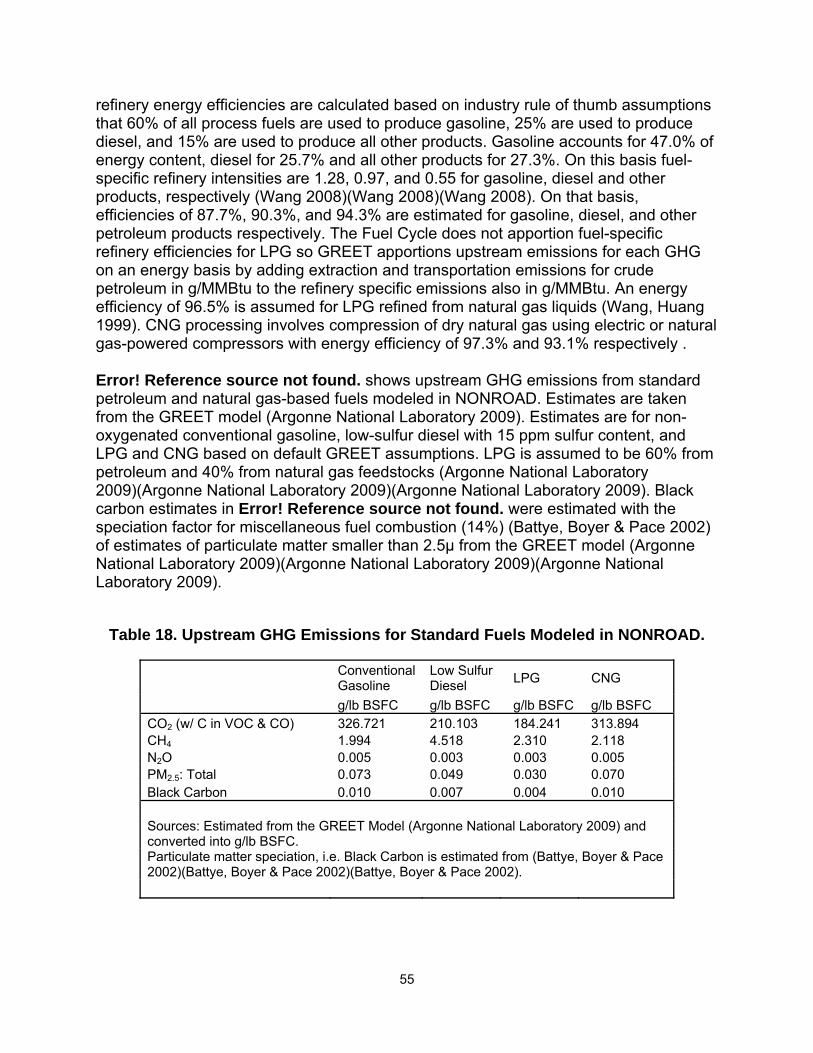
55
refinery energy efficiencies are calculated based on industry rule of thumb assumptions that 60% of all process fuels are used to produce gasoline, 25% are used to produce diesel, and 15% are used to produce all other products. Gasoline accounts for 47.0% of energy content, diesel for 25.7% and all other products for 27.3%. On this basis fuel-specific refinery intensities are 1.28, 0.97, and 0.55 for gasoline, diesel and other products, respectively (Wang 2008)(Wang 2008)(Wang 2008). On that basis, efficiencies of 87.7%, 90.3%, and 94.3% are estimated for gasoline, diesel, and other petroleum products respectively. The Fuel Cycle does not apportion fuel-specific refinery efficiencies for LPG so GREET apportions upstream emissions for each GHG on an energy basis by adding extraction and transportation emissions for crude petroleum in g/MMBtu to the refinery specific emissions also in g/MMBtu. An energy efficiency of 96.5% is assumed for LPG refined from natural gas liquids (Wang, Huang 1999). CNG processing involves compression of dry natural gas using electric or natural gas-powered compressors with energy efficiency of 97.3% and 93.1% respectively . Error! Reference source not found. shows upstream GHG emissions from standard petroleum and natural gas-based fuels modeled in NONROAD. Estimates are taken from the GREET model (Argonne National Laboratory 2009). Estimates are for non-oxygenated conventional gasoline, low-sulfur diesel with 15 ppm sulfur content, and LPG and CNG based on default GREET assumptions. LPG is assumed to be 60% from petroleum and 40% from natural gas feedstocks (Argonne National Laboratory 2009)(Argonne National Laboratory 2009)(Argonne National Laboratory 2009). Black carbon estimates in Error! Reference source not found. were estimated with the speciation factor for miscellaneous fuel combustion (14%) (Battye, Boyer & Pace 2002) of estimates of particulate matter smaller than 2.5μ from the GREET model (Argonne National Laboratory 2009)(Argonne National Laboratory 2009)(Argonne National Laboratory 2009).
Table 18. Upstream GHG Emissions for Standard Fuels Modeled in NONROAD.
Conventional Gasoline
Low Sulfur Diesel LPG CNG
g/lb BSFC g/lb BSFC g/lb BSFC g/lb BSFC CO2 (w/ C in VOC & CO) 326.721 210.103 184.241 313.894 CH4 1.994 4.518 2.310 2.118 N2O 0.005 0.003 0.003 0.005 PM2.5: Total 0.073 0.049 0.030 0.070 Black Carbon 0.010 0.007 0.004 0.010 Sources: Estimated from the GREET Model (Argonne National Laboratory 2009) and converted into g/lb BSFC. Particulate matter speciation, i.e. Black Carbon is estimated from (Battye, Boyer & Pace 2002)(Battye, Boyer & Pace 2002)(Battye, Boyer & Pace 2002).

56
Biofuels
Biofuels are considered renewable because the CO2 emission from their combustion represents the release of sequestered carbon from the atmosphere and not fossil carbon such as petroleum, natural gas, or coal. Fossil fuels contribute to global warming by returning carbon to the atmosphere that has remained outside of the carbon cycle for millions of years (Wayne 1991)(Wayne 1991)(Wayne 1991). Biofuels have in common that they are produced from farmed vegetable matter or waste food products and go through a refining process in which the food product is prepared and converted into finished fuel (Huo et al. 2008)(Huo et al. 2008)(Huo et al. 2008). The refining processes include fermentation and gasification with processing into higher hydrocarbons through the Fischer-Tropsch process (Wu, Wu & Wang 2005). These processes are made more efficient by coproduction of steam, electricity or other products. Under the final EPA National Renewable Fuel Standard Program regulations concerning the inclusion of biofuels in transportation fuels and minimum GHG reduction standards for biofuels apply to off-road equipment (EPA 2010b). Corn and sugar cane-based ethanol, biodiesel from soy and waste grease, oil, and fats meet the new standard. Cellulose-based biofuels meet and often exceed the new standard. The regulation mandates that minimum proportions of fuel produced by refiners to be from cellulosic biofuel (0.004%) biomass-based diesel (1.10%), total advanced biofuel (0.61%), and renewable fuel (8.25%).8 Farming Emissions.
The upstream GHG footprint of biofuels includes emissions from farming of feedstocks including machinery, fertilizer and pesticide, and transportation of inputs. The GREET model (Argonne National Laboratory 2009) addresses biofuels produced from corn, corn stover i.e. leaves and stalks, woody and herbaceous biomass generically, bagasse or sugar cane straw, soybeans, and wood residue from forestry operations. Error! Reference source not found. shows emissions for ethanol production for each biomass input addressed in the GREET model. The differences among feedstocks reflect differences in the farming process because refining emissions were held constant.
Table 19. Upstream GHG Emissions for Ethanol from Biomass Feedstocks.
Corn Woody
Biomass Herbaceous Biomass
Corn Stover
Forest Residue Bagasse
g/lb BSFC
g/lb BSFC g/lb BSFC
g/lb BSFC
g/lb BSFC g/lb BSFC
CO2 (w/ C in VOC & CO) -236.321
-1082.581 -884.942 -828.921 -677.020 -729.703
CH4 1.260 -0.004 0.088 0.067 0.323 3.840
8 Proportions are for 2010, except biomass-based diesel, which is combined 2009-2010. These proportions will increase annually through 2022.

57
N2O 0.478 0.167 0.486 0.133 0.138 0.304 PM2.5: Total 0.226 0.095 0.097 0.096 0.149 5.304 Black Carbon 0.032 0.013 0.014 0.013 0.021 0.743 Sources: Estimated from the GREET Model (Argonne National Laboratory 2009) and converted into g/lb BSFC. Particulate matter speciation, i.e. Black Carbon is estimated from (Battye, Boyer & Pace 2002)(Battye, Boyer & Pace 2002)(Battye, Boyer & Pace 2002).
There is considerable variation in farming emissions for biofuel feedstocks. Error! Reference source not found. shows GHG and black carbon emissions for ethanol produced from the six types of biomass modeled for ethanol production in the GREET model (Argonne National Laboratory 2009). For compatibility with NONROAD all emissions are expressed in grams per pound of fuel. CO2 emissions are negative in each case which indicates that between the farming process and displacement of fossil fuel consumption through coproduction of fuels and other products, enough carbon is sequestered in the soil and there are sufficient CO2 savings from electricity or steam coproduced to more than offset the CO2 emissions associated with farming, transporting, producing, and distributing ethanol. Ethanol production produces the largest CO2 savings from woody biomass and the smallest from corn. Herbaceous biomass, corn stover, and bagasse are somewhat similar in this respect. Emissions from ethanol production from corn are generally higher than the alternatives except for particulate matter and CH4 from bagasse and N2O from herbaceous biomass. Much of the variation associated with farming of biofuel feedstocks results from emissions from the soil. Perennial plants such as switchgrass tend to fix carbon in the soil while annual plants such as corn tend to release carbon as CO2 from the soil (Wu, Wu & Wang 2005, Andress 2002). Residual agricultural materials such as corn stover would alternatively be left to decompose returning nutrients so that their use requires additional fertilizer inputs with increased N2O emissions (Wu, Wang & Huo 2006)(Wu, Wang & Huo 2006)(Wu, Wang & Huo 2006). Crop choice may also be a factor in farming emissions. Direct N2O emissions from biomass are a result of fertilizer application and nitrogen that is released as above ground biomass decomposes (Huo et al. 2008). Legumes such as soybeans fix nitrogen in the soil although this effect is not considered by IPCC because of the high level of uncertainty concerning the impact on N2O emissions (Huo et al. 2008). This reduces the need for application of nitrogen fertilizers to legumes, in contrast to other annual crops such as corn, which do not fix nitrogen in the soil. Corn requires fertilizer inputs of 420g per bushel compared to soybeans 62g per bushel. The total nitrogen left in field after harvest for soybean biomass is 200.7g per bushel compared with 141.6g per bushel for corn. In 2006 IPCC estimated that 0.01 kg of N2O is released into the atmosphere for every kg of elemental nitrogen as direct emissions with a range of from 0.003 to 0.03 (Huo et al. 2008). Indirect N2O emissions include volatilization and leaching of nitrates in the soil accounting for 0.00325 kg of N2O for every kg of elemental nitrogen in the soil, again with considerable uncertainty (0.0025-0.075) (Huo et al. 2008).

58
The production of biofuels results in varying levels of changes in land use. There is considerable uncertainty as to the extent of these changes (Liska, Perrin 2009). Direct emissions occur as a result of conversion of forest or pastureland to farmland, and are relatively straightforward to estimate. Indirect emissions result from economic shifts due to the increased competition for agricultural resources. Although there is evidence of the relationship, such as a correlation between the lower soybean prices and deforestation in Brazil, it has been argued recently that a consensus as to the magnitude of these effects from a sufficiently broad methodological base does not exist (Liska, Perrin 2009). A study that was partially funded by Argonne National Laboratory used an econometric land use modeling approach to address direct CO2 emissions from conversion of forests and pastureland to farming (Tyner et al. 2010). The study addresses CO2 emissions from US ethanol production from corn grown on a global scale due to shifts in land use. The study estimates an effect, and demonstrates that the effect is mitigated somewhat when population and yield increases are accounted for. Corn-based ethanol production is shown to have a smaller well-to-wheels GHG footprint than gasoline (Tyner et al. 2010). Corn is used to model ethanol production. The GREET model only addresses soybeans as a feedstock for biodiesel (Argonne National Laboratory 2009)(Argonne National Laboratory 2009)(Argonne National Laboratory 2009).

59
Process Emissions.
The other factors in the differences among biofuels emissions are displacement or energy savings from co-products or byproducts and emissions from refining the finished fuels. We compare standard fossil fuels modeled in NONROAD with biomass-based alternatives. The GREET model (Argonne National Laboratory 2009) does not include biomass alternatives for CNG or LPG. Alternatives are discussed for gasoline and diesel. Three processes are considered here including ethanol production, biodiesel production, and Fischer-Tropsch synthesis. Ethanol production is accomplished through the biological fermentation of biomass (Wu, Wu & Wang 2005)(Wu, Wu & Wang 2005)(Wu, Wu & Wang 2005). Biodiesel production involves the removal of oxygen from fats and oils leaving hydrocarbons of the desired size. These may include seed oils, recycled oils, or animal fats, but typically the feedstock for biodiesel is soybean oil in the United States. Two processes are described as standard (Huo et al. 2008). Transesterification is a reaction of triglyceride with ethanol or methanol to produce methyl esters (biodiesel) and glycerin at a weight ratio of roughly 5:1. Hydrotreating includes two subprocesses. Hydrodeoxygenation involves reaction of hydrogen with fatty acids yielding a paraffin and water. Decarboxylation involves extraction of CO2 using a lead/hydrogen catalyst. The Supercetane process is a hydrotreating technique that occurs in conjunction with hydrocracking so that large molecules are broken apart while oxygen is removed. This process produces 70-80% middle distillates, but also naphtha, and waxes as well as fuel gas for steam but not electricity production (Huo et al. 2008)(Huo et al. 2008)(Huo et al. 2008). A second hydrotreating process is a reaction of the bio-feedstock with hydrogen and steam to produce biodiesel with propane as a co-product (Huo et al. 2008)(Huo et al. 2008)(Huo et al. 2008). The Fischer-Tropsch (FT) process is addressed extensively in the GREET model (Argonne National Laboratory 2009) which is a testament to its extreme flexibility. The FT process can be applied to natural gas (Wang, Huang 1999)(Wang, Huang 1999)(Wang, Huang 1999), coal, or biomass (Kreutz, Larson & G. Williams 2008). The FT process involves breaking a feedstock down through cracking and partial oxidation to CO and hydrogen gas. The resulting syngas is then cleansed of its acid components i.e. H2S, CO2, and COS. The cleansed syngas is then reassembled into larger hydrocarbons, known as syn-crude, which may be refined into its components. Typically a number of components of different weights are produced including diesel, but also naphtha and potentially gasoline (Wu, Wu & Wang 2005). Although the GREET model (Argonne National Laboratory 2009)(Argonne National Laboratory 2009)(Argonne National Laboratory 2009) addresses fuel pathways separately much of the supporting literature describes coproduction and other emissions savings measures. Ethanol fermentation is combined with production of electricity through steam and natural gas turbines that use syngas, or other fuels produced through the Fischer-Tropsch process (Wu, Wu & Wang 2005). Biodiesel production may also include coproduction of steam or electricity (Huo et al. 2008).

60
These include FT diesel, FT naphtha, and FT gasoline, the latter of which is not modeled in GREET as it is not economically viable because of the energy intensity of gasoline blending (Wu, Wu & Wang 2005). FT naphtha can be marketed more profitably as a feedstock for petrochemical processes than as a blendstock for gasoline (Kreutz, Larson & G. Williams 2008). Again, no biofuel alternatives to CNG and LPG are addressed by the GREET model (Argonne National Laboratory 2009). We evaluate ethanol as an additive and as an alternative to gasoline. Because Fischer-Tropsch gasoline is not commercially viable we do not discuss it as an alternative to conventional or reformulated gasoline (Wu, Wu & Wang 2005). Biogasoline is discussed as a co-product or alternative product for biodiesel through hydrocracking, however the authors acknowledge that biogasoline is less ready for market than biodiesel (Huo et al. 2008). The GREET model does not address either of these two alternative gasoline pathways (Argonne National Laboratory 2009). We evaluate biodiesel and Fischer-Tropsch diesel as alternatives to diesel fuel. To evaluate Fischer-Tropsch synthesis we compare upstream emissions associated with Fischer-Tropsch diesel from biomass, natural gas, and coal feedstocks. Gasoline and Alternatives.
The GREET model (Argonne National Laboratory 2009) addresses conventional and reformulated gasoline, ethanol, and ethanol blends to run in spark ignition engines. The ethanol used in the model was produced from corn through fermentation. Corn was chosen as feedstock because it represents the most likely source for new ethanol use. It is however a worst case scenario for ethanol production minimizing CO2 sequestration. We compare GHG and black carbon emissions from production of conventional or unblended gasoline with reformulated gasoline, which is a 10% ethanol mixture. In addition we compare an 85% ethanol/gasoline mixture and 100% ethanol, both of which require dedicated engines. We converted the GREET model output from grams per MMBtu to grams per pound of gasoline equivalent on an energy basis. The modeling results are shown in Error! Reference source not found..
Table 20. Upstream Emissions from Gasoline, Ethanol, and Blends.
Conventional Gasoline
Reformulated Gasoline 10% Ethanol Blend
85% Ethanol Gasoline mix
100% Ethanol
(Requires Dedicated Engine) g/lb BSFC g/lb BSFC g/lb BSFC g/lb BSFC CO2 (w/ C in VOC & CO) 326.723 276.288 -192.660 -380.968 CH4 1.994 1.991 2.021 2.031 N2O 0.005 0.055 0.567 0.770 PM2.5: Total 0.073 0.091 0.287 0.365 Black Carbon 0.010 0.013 0.040 0.051
61
Sources: Estimated from the GREET Model (Argonne National Laboratory 2009) and converted into g/lb BSFC. Particulate matter speciation, i.e. Black Carbon is estimated from (Battye, Boyer & Pace 2002).
Ethanol production as shown in Error! Reference source not found. has negative upstream CO2 emissions of roughly the same rate as positive upstream CO2 emissions from gasoline refining. This means that carbon sequestration and displacement offset all emissions from ethanol production and roughly the same CO2 emissions that gasoline production produces. Upstream CH4 emissions increase slightly from substitution of ethanol for conventional gasoline however N2O and black carbon emissions increase substantially. Upstream N2O emissions from corn-based ethanol production are 154 times greater than from gasoline production. At nearly one thousandth the mass of CO2 sequestrated N2O emissions offset more than 30% of the benefits of CO2 sequestration due to the higher global warming potential of N2O. Upstream black carbon emissions from corn-based ethanol are four times higher than emissions from gasoline production. When substituted for conventional gasoline, reformulated gasoline with 10% ethanol reduces upstream CO2 emissions by 15%, with a modest increases in N2O and black carbon. The reduction of upstream GHG emissions from an 85% ethanol blend is greater than for reformulated gasoline. Reformulated gasoline is compatible with existing technology, as is the 85% ethanol blend if the vehicles have flex-fuel technology. However use of gasoline fuel in construction equipment is generally a small component limited to smaller engines. GREET models gasoline use in on-road vehicles, where ethanol shows modest improvements in emissions. Low Sulfur Diesel and Alternatives.
For 2010 the GREET model addresses low sulfur diesel as the baseline diesel fuel. For compatibility with NONROAD, 15 ppm sulfur content was specified instead of the 11 ppm GREET model default. The diesel alternatives considered were 20% biodiesel, low sulfur diesel mix, and FT diesel from natural gas, coal, and biomass feedstocks. DME was considered but unlike the other fuels DME will not work with standard compression ignition technology and showed CO2 and CH4 upstream emissions that were higher than low sulfur diesel.. Best case scenarios were modeled for the FT diesel fuels from all three feedstocks including steam or electricity export and CO2 sequestration in the case of coal. Both the GREET model and the literature (Kreutz, Larson & G. Williams 2008) are clear that upstream emissions from coal production without CO2 sequestration are prohibitively high. Error! Reference source not found. shows upstream emissions for low sulfur diesel and substitutable alternatives. FT diesel production from biomass feedstock with electricity export sequesters or displaces all three GHGs, massively in the case of CO2 and produces little black carbon. Independent of its availability it is the most environmentally friendly alternative that will work in standard compression ignition engines. The 20% biodiesel blend had the next lowest upstream CO2 emissions of the five diesel pathways modeled. Substitution of 20% of the low sulfur diesel with biodiesel reduced upstream emissions by 92%. If we

62
extrapolate CO2 emissions to 100% biodiesel the upstream emissions would clearly become negative. Biodiesel as modeled with the GREET model produces less CH4 than low sulfur diesel but more N2O and black carbon. Upstream GHG emissions of CO2 and CH4 from FT diesel are lower than the baseline when coal is the feedstock but higher when the feedstock is natural gas. All FT diesels are sinks for N2O. As modeled alternative biomass diesel fuels offer the possibility of massive carbon sequestration and displacement of fossil fuels. FT diesel from coal would reduce CO2 emissions by 59% and significantly lower the GHG impact of diesel fuel production if substituted for low sulfur diesel.
Table 21. Upstream Emissions from Low Sulfur and Alternative Diesel Fuels.
Baseline Low Sulfur Diesel
20% Biodiesel/Low Sulfur Diesel Mix
FTD Natural Gas Feedstock steam export
FTD Coal Feedstock w/ CO2 seq. electricity export
FTD Biomass Feedstock elect export
g/lb BSFC g/lb BSFC g/lb BSFC g/lb BSFC g/lb BSFC
CO2 (w/ C in VOC & CO) 287.966 23.657 291.248 117.017 -3542.944
CH4 1.944 1.730 3.539 4.353 -2.936 N2O 0.005 0.041 -0.002 -0.002 -0.023 PM2.5: Total 0.145 0.491 0.235 0.262 0.013 Black Carbon 0.020 0.069 0.033 0.037 0.002 Sources: Estimated from the GREET Model (Argonne National Laboratory 2009) and converted into g/lb BSFC. Particulate matter speciation, i.e. Black Carbon is estimated from (Battye, Boyer & Pace 2002). Procedure for Building GASCAP Dataset
The following procedure was used to develop the database of construction and related equipment modeled in NONROAD (EPA 2008a) by function, fuel and operating cycle, and power rating. Appendix B shows equipment function, power rating, average load, BSFC, and emissions of CO2, CH4, N2O, and black carbon from upstream and direct emissions. The procedure is as follows:
• Non-recreational equipment was identified from a list of NONROAD source classification codes (SCC) (EPA 2005d). The list was purged of equipment types that are strictly speaking specialty functions such as oil drilling, farming, airport activities, and so on.
• A script was written for NMIM which specified for each type of equipment by functional description, fuel cycle, (SCC) and power rating specifying year of manufacture as 2010, number of machines and hours of operation as one assuming the average of all technology types for the year. Distribution of the hour of operation was even across all twelve calendar months.
• NMIM was run at the county level with Middlesex County, NJ specified with fuel assumptions for 2010 and PM10, PM2.5, CO, NMOG, CO2, NH3, NOX, and SO2 as

63
the pollutants. This produced an error log that included errors for equipment specifications that were not produced in 2010 and winter equipment for which NONROAD has data for December through February only. The seasonal errors were corrected by distributing an hour of production over the three months of data. The errors for non-existent equipment types were ignored as these produced no records.
• NMIM was run with the corrected script for TOG and NMOG. The two databases were consolidated into a single database with TOG and NMOG variables. Evaporative and recycling emissions were consolidated into exhaust records for NMOG. This step does not exclude CH4 from fugitive emissions because fugitive emissions from gasoline are unaltered hydrocarbons, none of which are CH4 (EPA 2005a). Output for hourly emissions for all pollutants and equipment types were converted to grams from short tons.
• Direct emissions of CO2 were calculated as the sum of CO2 measured by NONROAD and the product of the combined exhaust and fugitive NMOG emissions and the ratio of carbon fraction for unburned fuel (0.87) and the carbon fraction of CO2 (12/44). Direct emissions of CH4 were calculated as the difference between TOG and NMOG. Direct emissions of N2O were calculated as the product of the emission factor (0.0074), the average power rating for the equipment class (EPA 2005d), and the appropriate load factor for the equipment class (EPA 2004b). Direct emissions of black carbon were calculated as the product of PM2.5 and the appropriate speciation factor.
• Adjusted BSFC was calculated as the product of the steady state BSFC, the appropriate TAF, and the average power rating for the class. Steady state BSFC, and the appropriate TAF were taken from the tables in Appendix A for spark ignition engines and Appendix B for compression ignition engines. The BSFCs shown express fuel consumption in grams per pound of fuel. All compression ignition engines already on the Tier 4 standards were assigned a TAF of 1.00. This was done with compression ignition engines 75 hp or smaller for 2010 models. See Table 15.
• Upstream emissions rates for standard fuels were taken from Error! Reference source not found. above. Error! Reference source not found. shows emission factors GHG and black carbon emission factors for standard fuels including CNG, LPG using the 60%/40% GREET model default ratio for natural gas and petroleum feedstock, conventional gasoline with no oxygenate, and low sulfur diesel. Upstream emission rates were converted to grams of emissions per pound of fuel consumed. Upstream emissions per hour are calculated as the product of the NONROAD BSFC and the GREET upstream emission factors.
• Upstream emissions for equipment types manufactured in 2010 are shown in Appendix C. Comparable data for 1988-2010 is included in GASCAP.
GASCAP Dataset Inputs and Outputs
Equipment inputs include equipment type, vintage, power rating, fuel type, and activity, for each equipment piece. Activity is assumed to be the product duration of equipment use in hours and average load taken from the NONROAD model. These inputs may be

64
macro assisted, however GASCAP will allow the user to override default load assumptions and type in different values. We are exploring ways to automate duration assumptions using macros as well. The equipment outputs include upstream, direct, and total emissions for CO2, CH4, N2O, and black carbon.
REVIEW OF MAINTENANCE AND REHABILITATION PROCEDURES FOR ROADWAYS AND BRIDGES
This section presents assumptions made for the GASCAP model about the lifetime maintenance and repair needs of roads and bridges constructed under New Jersey Department of Transportation (NJDOT) authority. These assumptions will provide the basis for estimating greenhouse gas (GHG) emissions attributable to transportation capital projects following construction. The full module has not been implemented in the current version of GASCAP as we identified various data sources that are needed to fully develop this method. This data is currently being analyzed by a group at NJIT and we are unable to obtain this data within the scope of the current project. We document work done prior to this finding in the section that follows. To the extent possible, both theory and evidence-based defaults were used to estimate the timing of maintenance and rehabilitation for asphalt and concrete pavement and for different types of bridges. Pavement defaults are taken from the New York State Department of Transportation (NYSDOT) Comprehensive Pavement Design Model (NYSDOT 2002)()(). Bridge defaults are taken from the Ohio Department of Transportation (ODOT) On-line Bridge Maintenance Manual Preventive Maintenance/Repair Guidelines for Bridges and Culverts (ODOT 2010), which is a website that lists maintenance and repair issues associated with bridges and the cost and expected service life of bridge repairs. New York State roadways are accepted as surrogates for New Jersey Roadways because of similarities in climate. Uncertainties connected with life-cycle cost analysis (LCCA) are greater with bridges than with pavement LCCA is not common practice for timing of maintenance and rehabilitation of bridges. The purpose of the defaults included in this report is to provide baseline defaults so that pavement and bridge engineers can have an easily modifiable basis from which to input lifetime assumptions into the GASCAP tool. The balance of this report elaborates the baseline assumptions for the expected lifetime, and maintenance and rehabilitation inputs of a facility over that lifetime. It begins with a review of the literature for LCCA discussing the data requirements, applicability and appropriateness for the GASCAP tool. The following section identifies maintenance and rehabilitation activities that will be included in the life time analysis feature of the GASCAP tool for roadways and bridges. Another section will present the structure of the life time emissions component of the GASCAP tool and a list of repair activities for roadways and bridges. It should be emphasized that maintenance and rehabilitation activities contribute extensively to the service life of a facility. However, this first version of the GASCAP tool will not be capable of adjusting the service life for maintenance and rehabilitation activities.
65
Prediction of Optimum Timing of Maintenance and Rehabilitation Activities
Economic analysis of life time costs are used as a means of rationalizing the decision-making process between alternative pavement and bridge designs. The life cycles of bridges and roads are quantified using LCCA. In general, these analyses compare costs over the lifetime of a facility from construction or reconstruction to reconstruction or demolition. Costs included are those associated with design, planning, construction, maintenance, rehabilitation and use for both pavement and bridges (Hawk 2003). For completeness, these costs are offset by salvage value, although the offset is minor. Because of the long planned service life of most of these facilities uncertainty associated with future costs of maintenance, rehabilitation, and costs to users, care is needed in interpreting results. One result of this seems to be that analysis of this type is more broadly accepted for pavement planning than bridge planning perhaps due to the longer service lives of bridges. These analyses are decision-making tools and as such are only for use as a part of the decision-making process. The history of the development of LCCA is outlined in thumbnail in a report to the Federal Highway Administration (Walls III, Smith 1998) and echoed in a report to NJDOT (Ozbay et al. 2003). The concept was outlined by the American Association of State Highway Officials (AASHTO) in 1960, although it was acknowledged that the information base to apply it with acceptable comprehensiveness and reliability did not exist at the time (Ozbay et al. 2003)(Ozbay et al. 2003)(Ozbay et al. 2003). In 1984 the National Cooperative Highway Research Program (NCHRP) and AASHTO reviewed and encouraged the use of LCCA as an economically-based decision support tool (Ozbay et al. 2003). However, it was not until 1991 under the Intermodal Surface Transportation Efficiency Act (ISTEA) that estimation of life cycle costs was required as part of the design and engineering of bridges, tunnels, and pavement projects for metropolitan and state transportation planning (Walls III, Smith 1998, Ozbay et al. 2003). In 1995 the National Highway System (NHS) Designation Act mandated LCCA for NHS projects valued at over $25 million. However, the regulations were relaxed in 1998 under the Transportation Equity Act for the 21st Century (TEA-21) when the mandate to conduct LCCA on NHS projects over $25 million was eliminated (Walls III, Smith 1998, Ozbay et al. 2003). TEA-21 left LCCA a voluntary but recommended component of transportation planning. FWHA policy emphasizes that LCCA is a tool that supports decision-making but the results should not be confused with the expert decisions of engineers (Walls III, Smith 1998, Ozbay et al. 2003). LCCA is the method of generating lifetime maintenance and rehabilitation plans described in the proposal for the Carbon Footprint Project. The proposal calls for assessment of the longevity of construction materials and carbon emissions associated with different maintenance protocols. Plans also call for use of estimates of vehicle volume to estimate the wear to the facility. LCCA, however, is not feasible at this time because of a lack of available data and historical information about deterioration and maintenance practices at NJDOT. It is also clear that LCCA is not standard practice for maintenance and rehabilitation planning for bridges (Markow, Hyman 2009).

66
The New York State Department of Transportation (NYSDOT) has produced detailed default expected life expectancy for preventive and remedial maintenance and rehabilitation of pavement. These defaults are used to assemble a default schedule for roadways with asphalt or concrete pavement for inclusion in the GASCAP tool. For bridges the default maintenance and rehabilitation schedule is limited to indentifying the inputs and suggesting a probable sequence of maintenance events, without considering the timing of activities. Maintenance and rehabilitation plans are included as defaults but we intend to build in substantial flexibility to allow GASCAP users to plan maintenance and rehabilitation based on their expertise. It bares emphasis that LCCA analyses are not generally accepted as a stand-alone basis for decision making among project alternatives. LCCA approaches are useful as a basis for estimating maintenance and rehabilitation inputs because those inputs must be specified as the basis for estimating cost. We classify GHG emissions from maintenance and rehabilitation as downstream emissions, despite the virtual certainty that they will be attributable to NJDOT or its agents, because these emissions are unrealized at the point of construction. Although LCCA is beyond the scope of what is feasible for the Carbon Footprint analysis, it provides a basis for evaluating alternative approaches to the timing of maintenance and rehabilitation of roadways and bridges. LCCA is economic analysis that compares the costs of alternative pavement and bridge designs, with future costs adjusted with a discount rate to account for opportunity costs. LCCA allows selection of an economically most efficient project. How LCCA Works
LCCA is a generalized method of estimating discounted present and future costs of constructing, rehabilitating and maintaining that is applied to transportation facilities. It is a response to a perceived need to rationalize the timing of preventive maintenance and rehabilitation (Walls III, Smith 1998). It is assumed that alternatives have the following known or assumed attributes: an expected design life, periodic maintenance treatments to meet that design life, and a set of rehabilitation activities (Walls III, Smith 1998). Design life refers to the time between construction and the end of serviceable life of a design alternative. It is the period of time during which the alternative design can be expected to deteriorate to the point that it is no longer useable or in other words, the point at which it reaches terminal serviceability. LCCA involves comparison of alternative project facility designs over a fixed analysis period. The analysis period should be long enough to reflect differences among design alternatives and should be long enough to accommodate at least one rehabilitation. FWHA guidance recommends a minimum analysis period for pavement of at least 35 years (Walls III, Smith 1998). Analysis periods shorter than 35 years are not discouraged if all alternatives reach terminal serviceability in less than 35 years. Analysis periods for bridges are generally much longer (Hawk 2003). The New Jersey Guidance suggests analysis periods of 25

67
to 40 years for new pavement, 5 – 15 years for pavement rehabilitation and 75 years or more for bridges, tunnels, and hydraulic systems (Ozbay et al. 2003). The life cycle cost (LCC) is the net present value of all costs (NPVC) associated with a transportation facility (Ozbay et al. 2003). These costs may be one-time costs such as the construction itself or rehabilitation costs if there is one rehabilitation included in the planned service life of an alternative. There may also be recurring costs such as routine maintenance and rehabilitation at fixed n year intervals (Hawk 2003, Ozbay et al. 2003). Generally this is expressed NPVC = T∑t=0 Ct * (1 + d)-t
where Ct is the non-recurring cost of a transportation project in year t and d is the discount rate. Costs that recur at regular intervals are useful in LCCA if the costs are common to all of the alternatives (Ozbay et al. 2003). The purpose of LCCA is to achieve long term economic efficiency in the comparison of alternative investments on a cost minimizing basis (Walls III, Smith 1998). For bridges and pavements, the LCC is given by the following equation (Hawk 2003): LCC = DC + CC + MC + RC + UC + SV where DC is the design cost; CC is the construction cost; RC is the rehabilitation cost; MC is the maintenance cost; UC is the user cost; and SV is the salvage value of the project. Design and construction costs generally occur before the beginning of the service life of a facility and are in year 0 and therefore are not discounted. Rehabilitation and maintenance costs occur between year 1 and year T – 1 and are discounted. These costs are stated under the assumption that treatments are timely as the cost-effectiveness of most treatments may be severely reduced when applied as an emergency measure on a deteriorated facility (Peshkin, Hoerner & Zimmerman 2004)(Peshkin, Hoerner & Zimmerman 2004)(Peshkin, Hoerner & Zimmerman 2004). User costs are generally complicated and difficult to assess. These include operating costs such as tolls, crash costs and delay costs (time) due to normal operations as facilities deteriorate, and also due to traffic restrictions that arise from repairs (Walls III, Smith 1998). User costs are generally not straightforward to calculate, and are often excluded from the analysis in practice (Ozbay et al. 2003). Their exclusion results in an LCC based solely on costs to the department of transportation. Salvage value is the value of the project at the end of its service life expressed as a negative cost that occurs in year T (Walls III, Smith 1998). On this basis the equation above may be rewritten as LCC = DC + CC + T∑t=0 ((MCt + RCt) * (1 + d)-t) + SV * (1 + d)-T
LCC computation is data intensive and subject to high uncertainty. The uncertainty factor is a result of predicting input parameters far into the future. The New Jersey guidance (Ozbay et al. 2003) recommends sensitivity testing for the discount rate,

68
timing of rehabilitation activities, traffic growth rates, costs associated with construction inputs, and the length of the analysis period. Fluctuation in construction inputs will affect maintenance and rehabilitation costs. Monte Carlo testing is widely recommended as a means to reduce risks from errors by presenting results as probabilities rather than as certainties as would be implied by the use of data points (Hawk 2003, Walls III, Smith 1998, Ozbay et al. 2003). LCCA Procedure for Pavement
The New York State Comprehensive Pavement Design Manual (NYSDOT 2002) section on LCCA defines department costs as those necessary to provide serviceable pavement over a selected analysis period including current treatment costs, costs, timing, and service lives of future maintenance and rehabilitation activities, the time value of money i.e. the discount rate and the salvage value. Budgetary constraints, non-pavement construction needs, and heavy traffic volumes are also mentioned as considerations in selection of a pavement alternative. The LCCA procedure is made up of the following steps as described in the New Jersey Guidance (Ozbay et al. 2003):
1. Define the project’s alternatives. 2. Choose a probabilistic or deterministic approach. 3. Choose the general economic parameters including the discount rate and
analysis period. 4. Establish an expenditure stream for each alternative. 5. Compute the NPV for each alternative. 6. Compare and interpret the results and conduct sensitivity analysis. 7. Reevaluate the design strategy if needed.
The New York State Comprehensive Pavement Design Manual (NYSDOT 2002) includes the same steps except step 2. NYSDOT like many other state transportation agencies (Ozbay et al. 2003) uses a deterministic approach, which is less data intensive because it does not include Monte Carlo testing procedures. The first step is to identify alternatives including all appropriate initial alternatives (NYSDOT 2002). Alternatives are based on inspection of facilities to identify distress types and severity, and conditions for use data associated with each treatment based on historical data for New York State. The analysis period should be long enough for one or two rehabilitation treatments and several preventive maintenance treatments. The analysis period should at a minimum cover the maximum expected service life of the initial construction and one rehabilitation treatment. The example presented used a 30 year analysis period for the alternatives considered. A discount rate of four percent is used. Rehabilitation and maintenance treatments are incorporated using the Preliminary Estimating Program (PEP) with regional data within New York State. Sensitivity analysis is performed on treatment service lives, treatment timing, future treatment strategies, and item costs, but not the discount rate. The procedure described above results in plausible assumptions regarding the service life of rehabilitation and maintenance treatments described below. These estimates are

69
stated as single values, not probabilities. It is not possible through the Carbon Footprint Project whether these values are reliably applicable to New Jersey. Neither is it possible to address the extent that any maintenance or rehabilitation treatment would extend the service life of a roadway in New Jersey with any validity. However, these treatments will make it possible to specify default maintenance and rehabilitation plans for the GASCAP spreadsheet. It is expected that design engineers at NJDOT will be able to use these defaults as a basis for lifetime maintenance and rehabilitation based on their own expertise. LCCA Procedure for Bridges
LCCA procedures for bridges have greater uncertainty that arises from the longer service lives of bridges. This problem was recognized in NCHRP documentation for a plan to develop LCCA software for bridges in 2003 (Hawk 2003), when it was stated that bridges as a general rule have perpetual service lives. Six years later another NCHRP report (Markow, Hyman 2009) reviewed bridge management practices in the United States and Canada. Based on survey data, most state DOTs use of bridge management system data is for current or near term analysis of bridge condition rather than long term analysis of economic costs. Standard practice for bridges involves needs assessment based on biennial bridge inspections (Markow, Hyman 2009). The GASCAP spreadsheet will assume this and offer a 75 year default analysis period with biennial inspections which users will be able to supplement with maintenance and rehabilitation treatments based on their expertise. GASCAP Approach to Lifetime Maintenance and Rehabilitation
The GASCAP tool will allow users to fill in an optional timeline for anticipated maintenance and rehabilitation of newly constructed or reconstructed roadways and bridges. Users will be asked to specify if they want to include a lifetime maintenance and rehabilitation plan, and if so the type of roadway or bridge and what the expected service life of the facility is. More detailed information will be required from the user on the timing and maintenance activities expected to be undertaken. The GASCAP tool will provide a simple framework for entering this information. We hope that after further consultations with NJDOT staff, we may be able to suggest some default maintenance plans. We are also planning meetings with staff at CAIT and NJIT who may be able to provide information or data on maintenance activities. The balance of this section lists maintenance and rehabilitation inputs that will be addressed by GASCAP. The emissions factors for the materials used in these treatments are readily calculated from the materials page in GASCAP; any emissions factors from the maintenance equipment emissions can also be calculated. The inputs needed by the user will be similar to other components of GASCAP, such as volume of material and hours of equipment use (much of which can be derived from associated bid sheets). The critical difference in how we deal with these items is that the user determines a lifetime maintenance schedule as part of the construction process, although we intend to report the results both in a combined and disaggregated format.

70
Maintenance and Rehabilitation of Roadways
For roadways and other structures, maintenance and rehabilitation are processes by which remedial steps are taken to counteract wear and distress due to weather, climate and traffic. This section briefly discusses the remedial steps taken to remedy the various types of deterioration for roadways. GASCAP users will be able to select these steps from a menu. Roadway treatments are taken from the NYSDOT Comprehensive Pavement Design Manual (NYSDOT 2002)(NYSDOT 2002)(NYSDOT 2002). Rigid Pavement Preventive Maintenance
Joint and Crack Filling. This procedure involves cleaning and filling longitudinal and transverse joints, slab cracks, and the pavement/shoulder joint. Expected service life is two years. Joint and Crack Sealing. This procedure involves cleaning and sealing longitudinal and transverse joints, routing cleaning and sealing slab cracks, and cleaning and filling the pavement/shoulder joint. Expected service life is eight years. Joint and Crack Sealing with Spall Repair. In this procedure spalls9 are milled and patched with rapid-setting concrete patching materials. Longitudinal and transverse joints are cleaned and sealed. Slab cracks are routed, cleaned and sealed. The pavement/shoulder joint is cleaned and filled. (See flexible shoulder treatments.) Expected service life is eight years for joint and crack repairs and ten years for spall repair. Rigid Pavement Corrective Maintenance
Joint and Crack Sealing with Spall Repair and Grinding. In this procedure spalls are milled and patched and joints and cracks are addressed as with joint and crack sealing with spall repair. In addition, rough areas in the concrete are ground. Expected service life is eight years for the joint and crack repairs, ten years for spall repair, and five years for the ground areas. Joint and Crack Sealing with Spall Repair, Grinding, and Full-Depth Segment Replacement. In this procedure rough areas are ground, spalls are milled and patched and joints and cracks are addressed as with joint and crack sealing with spall repair, and grinding. In addition, one or more of the Portland concrete segments is replaced. Expected service life is eight years for joint and crack repairs, ten years for spall repair, and five years for grinding. Full-depth replacement segments are expected to equal or exceed the remaining life of the existing rigid pavement for as long as thirty years.
9 Spalling is a process by which chips or flakes are removed from concrete.
71
Rigid Pavement Rehabilitation
Joint and Crack Sealing with Spall Repair and Full-Depth Segment Replacement. In this procedure spalls are milled and patched and joints and cracks are addressed as with joint and crack sealing with spall repair. In addition, one or more of the original Portland concrete segments is replaced. Expected service life is eight years for joint and crack repairs, and ten years for spall repair. Full-depth replacement segments are expected to equal or exceed the remaining life of the existing rigid pavement for as long as thirty years. Bonded Concrete Overlay. Under this procedure pavement is scarified10 to a depth of 0.25 in. by sandblasting, after spalls are milled out. The pavement is cleaned and a 3” Portland concrete bonded overlay is applied. When hard the overlay is sawed and sealed over the existing joints. Asphalt or Portland concrete may be used for the shoulder. Expected service life is 20 years. Required maintenance includes joint and crack resealing every eight years. Sawed and Sealed Asphalt Concrete Overlay 3”. Under this procedure there may be partial full-depth replacement of segments with Portland concrete or asphalt concrete. Spalls are milled and patched with rapid-setting Portland concrete or asphalt concrete. Joints and cracks including the pavement/shoulder joint are cleaned and filled. Faults and wheel ruts are shimmed11 and the pavement is cleaned. A tack coat is applied to the surface. Asphalt concrete is applied to level the surface followed by two 1.5” lifts that include a binder and surface layers. The rehabilitated pavement is sawed and sealed over the existing transverse joints. Expected service life is 15 years for the 3” asphalt overlay with full length transverse crack sealing every five years as required maintenance. The expected service life for the sawed and sealed joints is eight years. Full depth asphalt concrete repairs will require bump milling every five years. Full depth Portland concrete repairs have an expected service life of 30 years. Sawed and Sealed Asphalt Concrete Overlay 4”. Under this procedure there may be partial full-depth segment replacement of segments with Portland concrete or asphalt concrete. Spalls are milled and patched with rapid-setting Portland concrete or asphalt concrete. Joints and cracks including the pavement/shoulder joint are cleaned and filled. Faults and wheel ruts are shimmed and the pavement is cleaned. A tack coat is applied to the surface. Asphalt concrete is applied to level the surface followed by three lifts. These include a 1.0” first course followed by a 1.5” intermediate course and a 1.5” surface course. Expected service life is 15 years for the 3” asphalt overlay with full length transverse crack sealing every five years as required maintenance. The expected service life for the sawed and sealed joints is eight years. Full depth asphalt concrete repairs will require bump milling every five years. Full depth Portland concrete repairs have an expected service life of 30 years.
10 Milled. 11 Shimming in this context refers to filling faults and wheel ruts to even out the pavement before an overlay is applied.
72
Asphalt Concrete Overlay (5”) Preceded by Cracking and Seating. Under this procedure there may be partial full-depth segment replacement of segments with Portland concrete or asphalt concrete. Non-replaced pavement is stabilized by cracking and seating. Spalls are milled and patched with asphalt concrete. Joints, including the pavement/shoulder joint and cracks are cleaned and filled. Faults and wheel ruts are shimmed. The pavement is cleaned and a tack coat is applied. The surface is then trued and leveled with asphalt concrete. Asphalt concrete is applied to level the surface followed by three lifts. Asphalt concrete is applied to level the surface followed by three lifts. These include a 2.0” initial course followed by a 1.5” intermediate course and a 1.5” surface course. The expected service life of the asphalt overlay is 15 years with required maintenance including full-length sealing of transverse cracks every five years. The service life for full depth repairs is 15 years for asphalt concrete and 30 years for Portland concrete. Asphalt Concrete Overlay (6”) Preceded by Rubblizing. This procedure begins with installation of an edge drain consisting of a “daylighted” crushed stone shoulder. Asphalt patches and overlays are removed, rubblized, and compacted. Depressions are patched with crushed stone. Asphalt concrete is applied to level the surface followed by three lifts. These include a 3.0” base course followed by a 1.5” intermediate course and a 1.5” surface course. No full-depth replacement or spall repair is required. The expected service life is 15 years with required maintenance including full-length sealing of transverse cracks every five years. Rigid Pavement Reconstruction
Full-Depth Portland Cement or Asphalt Concrete. This procedure includes full removal and replacement of pavement. The service life for full reconstruction is 15 years if the replacement material is asphalt concrete and 30 years if replacement is done with Portland concrete. Flexible Pavement Preventive Maintenance
Crack Sealing. Under this procedure transverse cracks are routed, cleaned and sealed. Pavement/shoulder joints are cleaned and filled. The expected service life is five years. Crack Filling. Under this procedure cracks and the pavement/shoulder joint are cleaned and filled. The expected service life is two years. Single-Course Overlay (1” to 1.5”). For this procedure cracks and the pavement/shoulder joint are cleaned and filled and the pavement is cleaned. A tack coat is applied before an asphalt concrete top course between 1” and 1.5” in depth. The expected service life is eight years. Maintenance consists of full-width transverse crack sealing after the first year and every five years thereafter, and filling of other cracks every two years starting after the second year.

73
Flexible Pavement Corrective Maintenance
Single-Course Overlay (1” to 1.5”). For this procedure severe cracks are milled and patched with asphalt concrete. Pavement/shoulder joints are cleaned and filled and wheel ruts are shimmed. The pavement is cleaned and a tack coat is applied. The pavement is trued and leveled with asphalt concrete and a surface course is applied between 1” and 1.5”. The expected service life is eight years. Maintenance consists of full-width transverse crack sealing after the first year and every five years thereafter, and filling of other cracks every two years starting after the second year. Hot In-Place Recycle (1” to 1.5”). The pavement is milled to a depth of 1” to 1.5”. A tack coat is applied before a surface course consisting of the recycled material is applied as hot mix asphalt concrete between 1” and 1.5”. The expected service life is eight years. Maintenance consists of full-width transverse crack sealing after the first year and every five years thereafter, and filling of other cracks every two years starting after the second year. Cold Milling and Replacement (1” to 1.5”). The pavement is cold milled to a depth of 1” to 1.5”. Severe cracks and raveled12 or stripped areas are patched with asphalt concrete. A tack coat is applied before a surface course of asphalt concrete between 1” and 1.5” is applied. The expected service life is eight years. Maintenance consists of full-width transverse crack sealing after the first year and every five years thereafter, and filling of other cracks every two years starting after the second year. Flexible Pavement Rehabilitation
Two-Course Overlay (3”). Severe cracks are milled and patched with asphalt concrete and cracks and the pavement/shoulder joint are filled. Wheel ruts are shimmed. The pavement is cleaned and a tack coat is applied. A truing and leveling course is applied followed by a 1.5” intermediate course and a 1.5” binding course. The expected service life is 15 years. Maintenance consists of full-width transverse crack sealing every five years, and filling of other cracks every two years. Cold Milling with Single-Course Overlay (3”). The pavement is cold milled to a depth of at least 1.5”. Severe cracks and raveled or stripped areas are milled and patched. A tack coat is applied followed by a course of asphalt concrete of at least 1.5”. A surface course of asphalt concrete is then applied to a depth of 1.5”. The milled material is transported to the dump or to a recycling facility. The expected service life is 15 years. Maintenance consists of full-width transverse crack sealing every five years, and filling of other cracks every two years. Hot In-Place Recycle with Single-Course Overlay (3”). The pavement is milled to a depth of 1.5”. A tack coat is applied before an intermediate course consisting of the recycled material is applied as hot mix asphalt concrete to a depth of 1.5”. A surface course is applied to a depth of 1.5”. The expected service life is 15 years. Maintenance 12 Raveling refers to loss of aggregate due to deterioration of the binding material.

74
consists of full-width transverse crack sealing every five years, and filling of other cracks every two years. Cold In-Place Recycle with Single-Course Overlay (4.5”). The pavement is milled and recycled to a depth of 3”, mixed as warm mix asphalt concrete and reapplied to a depth of 3”. An asphalt concrete top course is applied to a depth of 1.5”. The expected service life is 15 years. Maintenance consists of full-width transverse crack sealing every five years, and filling of other cracks every two years. Multiple-Course Overlay (≥4”). Under this procedure severe cracks are milled and patched and pavement/shoulder cracks are cleaned and filled with asphalt concrete. Wheel ruts are shimmed. The pavement is cleaned and a tack coat and truing and leveling course are applied. An asphalt concrete strengthening course from 1” to 4” is applied, followed by a 1.5” intermediary course. The surface course is applied to a depth of 1.5”. The expected service life is 15 years. Maintenance consists of full-width transverse crack sealing every five years, and filling of other cracks every two years. Cold Milling with Multiple-Course Overlay (≥4”). The existing pavement is milled to a depth of at least 1”. Raveled and stripped areas are patched with asphalt concrete and a tack coat is applied. An inlay or strengthening course at least 1” in depth is applied. Multiple lifts are needed if this course is greater than 4” in depth. An intermediate course of 1.5” is applied followed by a 1.5” surface course. The expected service life is 15 years. Maintenance consists of full-width transverse crack sealing every five years, and filling of other cracks every two years. Cold In-Place Recycle with Multiple-Course Overlay (6”). The pavement is milled and recycled to a depth of 3”, mixed as warm mix asphalt concrete and reapplied to a depth of 3”. A tack coat and a truing and leveling course are applied. An asphalt concrete intermediary course and a top course are applied, both to a depth of 1.5”. The expected service life is 15 years. Maintenance consists of full-width transverse crack sealing every five years, and filling of other cracks every two years. Flexible Pavement Reconstruction
Asphalt Concrete Pavement Construction above Existing Grade. This procedure involves scarification of the existing pavement and shoulder, construction and compaction of new fill and sub-base, and construction of new pavement and shoulder. This process can only be used where it is acceptable to raise the surface of the new pavement at least 12” above the surface of the old. The expected service life is 15 years. Maintenance consists of full-width transverse crack sealing every five years. Full-Depth Portland or Asphalt Concrete. This procedure includes full removal and replacement of pavement. The service life for full reconstruction is 15 years if the replacement material is asphalt concrete and 30 years if replacement is done with Portland concrete.
75
Flexible-over-Rigid Pavement Preventive Maintenance
Joint and/or Crack Sealing. This procedure requires that transverse joints and full-width transverse cracks be routed13, cleaned and sealed. Cracks in the pavement/shoulder joint are cleaned and filled. The expected service life of this procedure is five years. Joint and/or Crack Filling. Transverse joints and cracks, and the pavement/shoulder joint are cleaned and sealed. The expected service life is two years. Single-Course Overlay (1” to 1.5”). See flexible pavement above. Flexible-over-Rigid Pavement Corrective Maintenance
Mill and Patch Joints and/or Cracks. Severe cracks are patched. A tack coat is applied to the horizontal and vertical faces and asphalt concrete patches are applied. The expected service life is five years. Single-Course Overlay (1” to 1.5”). See flexible pavement above. Hot In-Place Recycle (1” to 1.5”). See flexible pavement above. Cold Milling and Replacement (1” to 1.5”). See flexible pavement above. Flexible-over-Rigid Rehabilitation
Two-Course Overlay (3”). See flexible pavement above. Cold Milling with Single-Course Overlay (≥3”). See flexible pavement above. Hot In-Place Recycle with Single-Course Overlay (3”). See flexible pavement above. Cold In-Place Recycle with Single-Course Overlay (4.5”). See flexible pavement above. Multiple-Course Overlay (≥4”). See flexible pavement above. Cold Milling with Multiple-Course Overlay (≥4”). See flexible pavement above. Cold In-Place Recycle with Multiple-Course Overlay (6”). See flexible pavement above.
13 Routing in this context refers to removal of material from a crack with a router to improve adhesion of filling material.

76
Remove Flexible Overlay, Crack and Seat with Multiple-Course Overlay (5”). This procedure requires that the existing asphalt concrete overlay be removed. The underlying Portland concrete pavement is cracked and seated. Spalls are milled and patched with asphalt concrete. Joints and cracks are cleaned and filled and faults and wheel ruts are shimmed. After cleaning a tack coat is applied to the pavement, followed by a truing and leveling course. Three courses of asphalt concrete are applied. The initial course is applied to a depth of 2” and the intermediate and surface courses are applied to a depth of 1.5” each. The service life of this procedure is 15 years with full-width transverse crack sealing every five years. Remove Flexible Overlay, Rubblize with Multiple-Course Overlay (6”). This procedure requires that the existing asphalt concrete overlay be removed. An underdrain is installed in the shoulder or the existing shoulder may be replaced with a daylighted crushed stone shoulder. 14 The underlying Portland concrete pavement is rubblized15 and compacted. Depressions are patched with crushed stone. Three courses of asphalt concrete are applied. The initial course is applied to a depth of 3” and the intermediate and surface courses are applied to a depth of 1.5” each. The service life of this procedure is 15 years with full-width transverse crack sealing every five years. Flexible-over-Rigid Reconstruction
Full-Depth Portland cement or Asphalt Concrete. This procedure includes full removal and replacement of pavement. The service life for full reconstruction is 15 years if the replacement material is asphalt concrete and 30 years if replacement is done with Portland concrete. Rigid or Flexible-over-Rigid Pavement Widening
Portland Cement Concrete. This procedure involves the excavation and removal of the existing shoulder, widening of the embankment and sub-base, and replacement and compaction of the new and disturbed sub-base. Holes are drilled and longitudinal joint ties are installed. Transverse load-transfer devices are placed. The Portland concrete is placed. Longitudinal and transverse joints are constructed, as is the new shoulder. The expected service life of the widened portion of the road is up to 30 years, and should equal or exceed the service life of the original part of the road. Joint sealing is required every eight years. Flexible or Flexible-over-Rigid Pavement Widening
Asphalt Concrete. This procedure involves the excavation and removal of the existing shoulder, widening of the embankment and sub-base, and replacement and compaction
14 A daylighted crushed stone shoulder uses crushed stone to channel water away from the roadway, preferably to an open place, i.e. daylight, where the water will not be able to accumulate. 15 Rubblization is a process by which concrete is broken up for use as aggregate.

77
of the new and disturbed sub-base. A tack coat is applied to the edge of the existing pavement. Asphalt concrete is placed and compacted and a longitudinal joint is routed and sealed. A new shoulder is constructed. The expected service life of the widened portion of the road is 15 years. Full width transverse crack sealing is required every five years. Flexible Shoulder Preventive Maintenance
Pavement/Shoulder Joint and/or Crack Filling. This procedure involves cleaning and filling cracks and the pavement/shoulder joint. The expected service life is two years. Surface Treatment. The shoulder is cleaned and a single surface treatment is applied. The expected service life is five years. Flexible Shoulder Corrective Maintenance
Asphalt Concrete Wedging. The shoulder is cleaned and a tack coat is applied. A wedge is created through the application of asphalt concrete adjacent to the pavement. The expected service life is three years. Surface Treatment. The shoulder is cleaned and a single surface treatment is applied. The expected service life is five years. Flexible Shoulder Rehabilitation
Single or Multiple-Course Asphalt Overlay. The shoulder is cleaned and a tack coat is applied. A single or multiple course overlay of asphalt concrete is applied. A single course overlay has an expected service life of eight years. A multiple course overlay has an expected service life of 15 years. Flexible Shoulder Reconstruction. Replacement may be with Portland concrete, asphalt concrete or bituminous-stabilized gravel with an asphalt concrete top course. The taper for a Portland concrete reconstruction is from 9” to 6”. For asphalt concrete reconstruction the shoulder is either 3” or 4”. For a bituminous-stabilized gravel reconstruction the bituminous-stabilized gravel is 3” and the top asphalt concrete course is 1”. A Portland concrete shoulder has an expected service life of 30 years, while an asphalt concrete or bituminous-stabilized gravel with asphalt top course each has 15-year expected service lives. Maintenance and Rehabilitation of Bridges
Bridges consist of the structural members, structural decks, and wearing courses that support vehicular traffic, as well as curbs, sidewalks, railings and fencing and utility pipes, conduits, lighting equipment and traffic signal hardware (AASHTO 2007). This section takes inputs from the On-line Bridge Maintenance Manual Preventive

78
Maintenance/Repair Guidelines for Bridges and Culverts (ODOT 2010), referred to as the Ohio guidance throughout the rest of this section. Maintenance and repair of bridges is significantly more complex than for road surfaces. We summarize various basic and common repairs as reported in the Ohio guidance; however, this can vary by specific circumstances. The Ohio guidance estimates costs for repairs in current dollars. We have included these values, however, we must also caution that the costs and expected service life estimates for the repairs listed here are based on data collected by ODOT, which may not be valid for New Jersey. We anticipate that the translation of this information into the GASCAP tool will require a more flexible approach rather than a complete menu of options. We hope that our upcoming meetings with NJDOT maintenance engineers will allow us to refine the bridge maintenance procedures. Abutments
Abutments provide structural support of bridge ends, bearing devices and backwalks. They are generally made of concrete. The seats are the flat parts of abutments that support the bearing devices. They are the most vulnerable part of these structures to deterioration from moisture and debris buildup. Wall type abutments support the structure from the stream bed. Stub abutments are shorter than the wall type and are built from the bank rather than the stream bed. Piles are normally driven to support stub abutments. Both structures have exposed seats. Routine maintenance includes power washing every year to remove salt and other deicing compounds and sealing the seats and adjacent parts of the faces every five years with silane/siloxane16 or every 15 years with epoxy/urethane17. Integral and semi-integral abutments encase the beam ends. Because these do not have exposed seats the need for preventive maintenance is greatly reduced. Integral abutments totally encase the beam ends which are connected with reinforcing steel. Semi-integral abutments are separated in the upper part from the expansion material. For stub type abutments leaning/tilting may be addressed by converting the abutment to integral abutments or replacement. The conversion repair is at a cost of $25,000 for each stub type abutment and has a serviceable life of 15 years. Replacement is at a cost of $50,000 for each stub type abutment. This repair has a serviceable life of 40 years. Settlement may be addressed by shimming with concrete, conversion to integral, or replacement. Raising the seat by shimming or with concrete is at a cost of $10,000 for each abutment and has a serviceable life of 15 years. Conversion to integral is at a cost of $20,000 for each stub type abutment. The repair has a serviceable life of 15 years. Replacement is at a cost of $50,000 for each stub type abutment. This repair has a serviceable life of 40 years. Concrete Deterioration is addressed by sealing of expansion joints and removal and patching of deteriorated concrete. Sealing of expansion joints costs approximately $150 per linear foot and has a service life of 15 years. Removal and patching of concrete is at a cost of $45 per square foot and has a service life of 15 years. 16 Commonly used commercially available concrete sealer. 17 Commonly used commercially available concrete sealer.

79
For wall abutments leaning may be addressed by tree cutting on the embankment at a cost of $500 per linear foot, Underpinning with concrete at a cost of $200 per linear foot, or replacement at $800 per linear foot. Service lives for these repairs are 10 years for tree removal, 15 years for underpinning, and 40 years for replacement. For exposed footers, if the abutment is not sitting on piling, underpin18 with concrete. In any case armor the footer with rock. With concrete underpinning the cost for this repair is $200 per foot, otherwise the cost is $20 per foot. In either case the expected service life of the repair is 15 years. For vertical cracking if the crack is wider than 3/8 inch fill with mortar or quick setting epoxy at a cost of $35 per linear foot. If the crack is less than 3/8 inch wide inject epoxy at a cost of $20 per linear foot. In either case the expected service life of the repair is 20 years. For deteriorated concrete repairs include sealing leaking joints, diverting scuppers, removing and patching unsound concrete at an overall cost of $45 per linear foot. The service life of these repairs is 20 years. For integral/semi-integral abutments if the crack is wider than 1/4 inch fill with mortar or quick setting epoxy at a cost of $35 per linear foot. If the crack is less than 1/4 inch wide inject epoxy at a cost of $20 per linear foot. In either case the expected service life of the repair is 30 years. For concrete deterioration repairs include placement of underdrains at $100 per linear foot and removal and patching of concrete at $45 per square foot. Underdrains have a serviceable life of 20 years and concrete patching has an expected serviceable life of 15 years. Approach Slabs
Approach slabs are the structures that connect the bridge to the roadway. They are generally built on disturbed earth that has been removed to place the backwall and abutments and are prone to settlement. Settlement is a problem because without a smooth transition from roadway to the bridge the bridge is susceptible to damage from impact, especially from heavy trucks. Preventive maintenance includes sealing the joint between the backwall and the approach slab with rubberized asphalt, and exclusion of groundhogs from the area. Scaling repairs may include sealing with silane at a cost of $2 per square foot, which has a serviceable life of five years or overlay with epoxy/sand slurry at a cost of $40 per SY, which has a serviceable life of ten years. Cracking repairs may include filling with epoxy and undersealing19 at a cost of $5 per linear foot, which has an expected serviceable life of 15 years or replacement of the approach slab at $60 per SY, which has an expected serviceable life of 30 years. Potholes may be repaired by saw cutting and replacing with quick setting concrete at a cost of $15 per SY with an expected service life of 10 years or filled with asphalt concrete at a cost of $2 per square yard and an expected service life of five years. Settlement may be addressed with an asphalt
18 Underpinning in this context means that concrete is added to an unstable footer to anchor it and provide stability. 19 Undersealing is a procedure whereby voids under approach slabs are filled by injection of grout through holes drilled for that purpose.

80
concrete overlay at $2 per SY with an expected service life of five years or mudjacked20 with grout or urethane at $15 per SY with an expected service life of 15 years. Arch Bridges
The Ohio guidance (ODOT 2010) discusses three types of arch bridge including filled spandrel21 wall arch bridge, the open spandrel arch, and the through arch or rainbow arch bridge. The filled spandrel wall arch bridge has a vertically curved concrete slab and vertical wall on top that form sides for the bridge. Granular material is used to fill the area defined by the arches and walls and support the road bed. Maintenance for these bridges is generally minimal, although the filled area tends to hold water, which can shift the fill material and cause cracking in the wearing surface. Sewer and water lines may fail contributing to problems with moisture. Preventive maintenance includes crack sealing the wearing surface, sealing gutter areas with rubberized asphalt or some other flexible sealer, routine inspection of buried utility pipes, and installation of drains if there is evidence of accumulation of moisture. Repairs of filled spandrel wall arch bridges include management of wall movement and repair of concrete deterioration. Generally sanitary, storm and water lines should be replaced if they are leaking and the berm area should be kept clear of vegetation. Moisture accumulation can be reduced by replacing the wearing surface at $10 per SY, crack sealing the surface at $2 per SY, Paving full width at $10 per linear foot and sealing the joint between the pavement edge and the wall face at $2 per linear foot. These are all ten-year repairs. Twenty-year repairs include drilling of weep holes at $50 each in the walls and $70 at low points in the arch. Installation of transverse tie rods between the walls at $1,000 each is also a twenty-year repair. Replacement of the walls at $1,500 per linear foot is a fifty-year repair. Deteriorated concrete is repaired by saw cutting and patching at $45 per square foot for a 25-year repair. Open spandrel arch bridges have vertically curved concrete slabs and vertical columns or arch ribs that support floor beams and the deck slab. Leakage at joints and drainage problems tend to cause damage from corrosion. The principal construction material is concrete. Preventive maintenance measures include sealing of concrete decks, annual cleaning and sealing of expansion joints, management of the drainage system so that drainage that falls onto the arch components is redirected. Repairs of open spandrel arch bridges include repairs to the wearing surface, floor beam deterioration, column deterioration and arch rib or ring deterioration. Open spandrel arch bridges have a concrete slab wearing surface which is discussed in the section on slab bridges. Floor beam, column, and arch rib deterioration are handled similarly. Floor beam deterioration that does not require replacement of the floor beams and deck may be repaired by patching delaminations and sealing joints at $45 per 20 Mudjacking involves insertion of a cement-based mixture to support structures undermined by settlement. 21 According to the Ohio Guidance spandrel bridges are supported by two arches from below. The filled spandrel wall arch bridge deck is supported by aggregate placed in the central area. Open spandrel arch bridges run columns between the arches and the deck for support.

81
square foot for a 20 year repair. Floor beam and deck replacement costs $80 per square foot and has an expected serviceable life of 40 years. Column or arch rib deterioration that is not severe is corrected by patching and sealing and adjusting drainage. It is not clear what the additional cost of replacing columns is. Bridge reconstruction costs $120 per square foot and has an expected serviceable life of 80 years. Rainbow arch bridges are supported by two arches that rise above the roadway and hold vertical columns which in turn support floor beams and the deck slab. Construction materials include reinforced concrete and steel. Because of slenderness of the vertical columns both the concrete and reinforcing steel components of reinforced concrete rainbow arch bridges are susceptible to corrosion from deicing materials. It is therefore necessary to have the splash zone cleaned and all its components sealed. Preventive maintenance includes annual power washing of the deck surface, gutters and vertical columns, sealing the concrete decks, sealing the arch within the splash zone with silane/siloxane or epoxy/urethane, and crack sealing the transverse contraction joints of the deck near each end with rubberized asphalt, silicone caulk, or urethane caulk. Repairs of rainbow arch bridges include repairs to the wearing surface, deck, floor beam deterioration, column deterioration and arch rib or ring deterioration. Repairs of the deck and wearing surface are referred to general guidance for those two issues. As with open spandrel arch bridges, less serious deterioration of the floor beams or arch ribs is treated by patching and sealing joints. Columns are fine structures and therefore difficult to patch, but can be reinforced. The guidance is not clear on the cost or expected life of reinforced columns. Backwalls
Backwalls are retaining walls at the bridge ends that support approach slabs directly and by holding back the embankment underneath the approach slabs. They are vulnerable to breakage from expanding pavement. Preventive maintenance includes power washing every year to remove deicing agents, sealing the backwall face with silane/siloxane every five years, or epoxy/urethane every 10 years, and installation of asphalt-filled relief joints to absorb the movement of expanding, usually concrete pavement. Repair issues include delaminations, leaning, and deterioration of the top portion. Delaminations are addressed by patching, and joint sealing at a cost of $45 per linear foot. No estimate of expected service life is included in the guidance. Tilting generally requires replacement of the backwall and adjustment of the beam ends. Simple replacement costs an estimated $600 per linear foot and has an estimated service life of 10 years. Moving the backwall away from the beam ends costs $800 per linear foot and has an estimated service life of 15 years. Conversion to integral abutments costs $1,000 per linear foot and has an estimated service life of 20 years. Repair of deteriorated tops involves bracing, if necessary, removal and replacement of deteriorated concrete, and installation of pavement pressure relief joints.
82
Beams
The beams covered by the Ohio guidance (ODOT 2010) are made either of steel or pre-stressed concrete. Pre-stressed concrete beams may be box beams or I-beams. Steel beams are subject to rust and more serious corrosion, bending through impact, and physical breaking. Pre-stressed concrete is subject to water damage, spalling, and cracking. For steel beams rust is managed by repainting. If less than 20% of the surface has lost its paint covering then it may be spot painted at $7.50 per square foot for a ten-year repair, otherwise the piece must be repainted at $5 per square foot for an 18-year repair. Repair of a steel beam that is seriously corroded involves plate over welding at $25 per square foot for a 10 year repair or addition of new steel by welding and grinding of the welds at $50 per square foot for a 30 year repair. Bent members may be heat straightened at $10,000 if less than six inches out of alignment or $5,000 per inch of deflection for a 25 year repair. Nicks and gouges are ground out so that sharp edges are eliminated. For concrete box beams leaking joints between beams are repaired by removing and replacing asphalt, waterproofing, and unsound grout at $15 per square foot for a 20 year repair. In cases of minor spalling without strand corrosion the concrete may be patched with mortar applied by trowel at a cost of $25 per square foot for a 20 year repair. If the spalling is more severe and there is strand corrosion then the beams must be replaced at a cost of $150 for a 40 year repair. Drip strips may be used to prevent damage from over-the-side drainage on the underside of outside beams at a cost of $5 per linear foot for a 30 year repair. Cracks may be treated with epoxy injection at $10 per linear foot for a permanent repair. For concrete I-beams cracks in the bottom flange may be treated by epoxy in injection at $10 per linear foot for a 20 year repair. Cracks in cast-in-place closure pour between beam ends may be treated the same way although replacement at $50 per cubic foot may also be necessary for a 20 year repair. Bearings
Bearings are devices that transfer weight from the superstructure to the substructure, and allow the bridge to expand and contract. They are usually constructed of steel or elastomeric neoprene, or a combination of both. They may be fixed, anchoring the superstructure to the substructure or sliding, rocker, or roller bearings, which allow movement. Preventive maintenance for steel or partial steel and neoprene bearings involves annual power washing, and painting with epoxy paint as needed. Preventive maintenance needs for neoprene bearings are minimal, consisting of an occasional power washing to prevent dirt and debris build-up.

83
The Ohio guidance (ODOT 2010) lists three repair issues for steel rocker type bearings: out of vertical, rust, and loose bearings. If a steel rocker bearing is out of vertical at 70o or less the bearing may be reseated and shimmed or the bridge may be jacked for a cost of $200 each and an expected service life of 10 years or the abutment may be converted to integral for a cost of $2,000 per linear foot and an expected service life of 30 years. To manage corrosion expansion joints should be resealed and the bearings should be painted at a cost of $80 per bearing and an expected service life of 15 years for the repair. Loose rocker bearings should be removed, cleaned and reseated and the expansion joint should be replaced or rehabilitated at a cost of $100 per linear foot of expansion joint and $1,500 per bearing. Expected serviceable life is 20 years for the expansion joint repair and 35 years for the rocker bearing repair. Repair issues for neoprene bearings include cracking, and repair of bearings that are loose or out of position. Cracked bearings may be sealed with silicone at $10 each for a 15 year repair, or replaced for a 40 year repair. Loose or out of position bearings should be reseated with shimming or grinding of the abutment as necessary. Reseating, including any shimming is at a cost of $50 per bearing. If the there is a need to grind abutments or piers there is an additional cost of $200. The expected service life of this repair is 15 years. Culverts
The Ohio guidance (ODOT 2010) describes culverts as structures that form a hole through an embankment. Corrugated metal pipe arch culverts are galvanized steel structures that are flat on the bottom and circular above that. Box culverts are precast concrete structures with three or four sides. Four-sided box culverts have a concrete bottom, while three-sided box culverts leave the ground exposed. Aluminum box culverts are three-sided corrugated aluminum structures. Three-sided culverts, whether precast concrete or aluminum must be seated on concrete platform at both ends. Generally preventive maintenance of culverts involves improving flow through placement of riprap, keeping the inside clear of debris, and removing trees and saplings as needed. The life of corrugated metal pipe arch culverts may be extended by adding a concrete bottom. Repairs for corrugated metal pipe arch culverts include correction of corrosion of the bottom platform, loss of shape, cracks at the bolted connections, scour hole at the outlet, and leaning at the headwall. Bottom corrosion may be addressed by laying concrete on the bottom at a cost of $100 per linear foot for a 20 year repair or replacement of the culvert at $1,200 per linear foot for a 35 year repair. Distortion of shape more than 15% may be remediable by installation of a liner plate at $1,000 per linear foot for a 35 year replacement or installation of a plastic liner at $800 per linear foot for a 40 year repair or the culvert may be replaced at $1,200 per linear foot for a 35 year repair. Trees may need to be removed at $0.50 each every 10 years or so. If cracks at the bolted connections involve more than 10% of the culverts length the problem may be addressed by welding rebar to every other corrugation at a cost of $50 each weld for a 10 year repair or the culvert may be replaced for $1,500 per linear foot

84
for a 25 year repair. Scour holes are addressed by placement of dump rock at the outlet. Disintegration or leaning of the headwall requires replacement of the headwall at a cost of $1,500 for a 30 year repair. Issues addressed for the repair of four-sided precast concrete box culverts include leaking joints, concrete disintegration, and gaps in the joints larger than one inch. Leaking joints may be excavated and the waterproofing replaced at a cost of $500 per linear foot for a 20 year repair or joint may be sealed with expanding polyethylene/urethane caulk or fast setting mortar at $10 per linear foot of joint for a 10 year repair. Deteriorated concrete may be addressed by sealing the joint at a cost of $10 per linear foot of joint and troweling mortar to patch, or gunite may be used for vertical and overhead areas, or a concrete slab may be laid onto the structure. The concrete or mortar repairs all cost $45 per square foot and have expected service lives of 15 years. Large gaps in the joints may be filled with fast setting mortar at a cost of $5 per linear foot of joint for a 10 year repair. Repairs for aluminum box culverts address leaking around seams and bolts, bulging or sagging of the top, and exposure or undermining footers. Leakage around seams and bolts is addressed by excavating and waterproofing these at a cost of $700 per linear foot. The Ohio guidance (ODOT 2010) does not specify the expected service life of this repair. Repair of bulging or sagging tops involves excavation of the culvert, jacking it back into shape and reseating it at a cost of $900 per linear foot for a 10 year repair or replacement of the culvert at $1,500 per linear foot for a 25 year repair. Undermined footers are underpinned with concrete. Undermined or exposed footers are armored with rock. The undermined footer repair cost is $100 per linear foot. The exposed footer repair is $25 per linear foot. The expected service life of both repairs is 15 years. Repairs for three-sided precast concrete culverts address leaking from joints, concrete delaminations, and exposure and undermining of footers. Joint leaks may be addressed from the underside by applying expanding urethane at a cost of $5 per linear foot of joint for a 15 year repair or by reapplying the waterproofing membrane at a cost of $200 per linear foot of culvert. Repair of concrete delaminations involves joint sealing and patching with mortar or gunite. Undermined or exposed footers are addressed as with aluminum box culverts above. Decks
In Ohio most reinforced concrete decks are 8.5 inches thick and sit on steel or concrete I-beams (ODOT 2010). There may or may not be a concrete overlay either 1.25 or 1.75 inches thick or an asphalt overlay 2.25 inches thick. The Ohio guidance (ODOT 2010) does not discuss steel grid decks and timber structures. The common features of reinforced concrete decks are discussed including wearing surfaces, sidewalks, railings, scuppers, drain pipes below the deck, over-the-side drainage, and expansion joints. Preventive maintenance for concrete decks and concrete overlays includes sweeping with a power broom, and power washing the gutter areas at least once a year to remove

85
deicing compounds and sealing the deck surface with silane or siloxane every five years. Transverse cracks should be filled with high molecular weight methacrylate or a gravity fed silicate solution. Ponding may be addressed by grinding a trough to draw drainage, or the low area may be patched. Delaminations, potholes, scaling and similar problems should be repaired and loose spalls removed. For asphalt overlays cracks should be sealed and more generalized weathering should be chip sealed or milled and filled with new asphalt. Slurry seals may also be used. Repairs for reinforced concrete decks include scaling, aggregate popouts, cracks including transverse cracks, potholes, and full-depth holes from the top side, and transverse cracks, delaminations, discolorations, and full-depth holes from the bottom side. Popouts and minor scaling or cracks may be addressed by sealing with silane at a cost of $1 per square foot for a five year repair. If scaling is deeper than ½ inch the deck should be milled to a depth of 1.25 inches and replaced with concrete inlay at a cost of $35 per square foot for a 15 year repair. More severe cracks may be treated with a high molecular weight Methacrylate (HMWM) at a cost of $2 per square foot for a 15 year repair, a reactive silicate solution at a cost of $0.50 per square foot for a five year repair, or with gravity fed resin at a cost of $1.50 per square foot for a ten year repair. Repair of potholes by patching involves removal of unsound material, saw cutting if concrete is the patching material and filling with asphalt or fast setting concrete patching material. The asphalt repair costs $15 per square foot and is a temporary repair with a three year expected service life. The concrete repair costs $100 per square foot and has an expected service life of 10 years. If more than 10% of the deck area is unsound it is recommended that the top surface of deck be removed and replaced with a 1.25 inch concrete inlay at a cost of $35 per square foot for a 15 year repair. An asphalt overlay may also be used as a temporary measure at a cost of $15 per square foot for a three to five year repair. Delaminations from under the bridge are not patched but may require that the deck be replaced. Full depth holes and discolorations may be replaced with a full depth concrete patch at a cost of $150 per square foot for a 10 year repair if less than 5% of the deck is missing or less than 10% of the deck is discolored, otherwise the deck should be replaced at a cost of $80 per square foot for a 40 year repair. Wearing surfaces may be either asphalt or concrete overlays. Repairs for asphalt overlays include cracks, surface raveling and potholes. Isolated cracks and less severe raveling may be treated by sealing with rubberized asphalt at a cost of $0.20 per square foot for a five year repair. If cracks are numerous or run together or if raveling asphalt is no longer bonded to the deck the affected section should be replaced with a waterproofing coat and new asphalt at a cost of $35 per square foot for a 10 year repair. If 15% or more of the wearing surface is covered with potholes they may be saw cut and patched with asphalt at a cost of $15 per square foot for a five year repair, otherwise the asphalt overlay should be replaced. Repairs for concrete overlays include scaling, popouts, cracking, delamination and potholes. Popouts and scaling less than ½ inch deep may be sealed with silane at a cost of $1 per square foot for a five year repair. Deeper scaling should be sounded, saw cut and patched with fast acting concrete patching material at a cost of $35 per square foot for a 15 year repair. Cracks may be treated with a high molecular weight Methacrylate (HMWM) at a cost of $2 per square

86
foot for a 15 year repair or with gravity fed resin at a cost of $1.50 per square foot for a ten year repair. Repair of potholes by patching involves removal of unsound material, saw cutting if concrete is the patching material and filling with asphalt or fast setting concrete patching material. The asphalt repair costs $15 per square foot and is a temporary repair with a three year expected service life. The concrete repair costs $100 per square foot and has an expected service life of 10 years. If more than 10% of the deck area is unsound it is recommended that the overlay be removed and replaced at a cost of $35 per square foot for a 15 year repair or that the deck should be replaced at a cost of $80 per square foot for a 40 year repair. Sidewalks on bridges are usually reinforced concrete although steel checkerplate is also used. The Ohio guidance (ODOT 2010) only addresses the reinforced concrete type. Preventive maintenance includes sweeping and power washing and sealing as with concrete decks. Cracks are handled as with concrete decks as well. However, care must be taken with sealers to add grit to ensure skid resistance and trip hazards must be addressed. Popouts and scaling of the surface may be corrected by cleaning and sealing with silane at a cost of $2 per square foot for a 10 year repair. Scaling may also be treated with a ¼ inch epoxy overlay at a cost of $35 per square foot for a 15 year repair. Cracks may be addressed with a high molecular weight methacrylate at a cost of $1 per square foot if the crack is less than 1/16 inch wide or by routing out the crack and applying a silicone or urethane caulk at a cost of $2.50 per square foot. Surface delaminations may be addressed by removing the unsound concrete, saw cutting the area and patching with patching material at a cost of $40 per square foot for a 15 year repair. If the deterioration is extensive saw cutting and full depth removal is necessary before recasting at a cost of $80 per square foot for a 30 year repair. Railings are walls on the sides of a bridge that prevent pedestrians and vehicles from going off the sides. They are usually either reinforced concrete or galvanized steel. Preventive maintenance for reinforced concrete railings includes power washing, especially inside the splash zone and sealing with silane or siloxane every five years. For reinforced concrete railings surface scaling or popouts may be addressed by sealing with silane or siloxane at $2 per square foot for a 10 year repair or epoxy/urethane at $4 per square foot for a 15 year repair. Cracks may be addressed with a high molecular weight methacrylate at a cost of $1 per square foot if the crack is less than 1/16 inch wide or by routing out the crack and applying a silicone or urethane caulk at a cost of $2.50 per square foot. Either is a 10 year repair. Surface delaminations may be addressed by removing the unsound concrete, saw cutting the area and patching with patching material at a cost of $40 per square foot for a 15 year repair or patching with a thin layer of trowel-applied mortar at $10 per square foot for a 10 year repair. If the deterioration is extensive, saw cutting and full depth removal is necessary before recasting at a cost of $80 per square foot or the railing may be replaced at $800 per linear foot. Either is a 30 year repair. Preventive maintenance of galvanized steel railings involves annual tightening of loose bolts and touching up with zinc paint. For galvanized steel railings if the railing is dented or gouged or anchor bolts become loose or imbedded repairs may include touch up with

87
zinc paint at a cost of $2 per square foot, replacement of guardrail sections at $25 per linear foot, or replacement of tubular backup sections at $80 per linear foot. The zinc paint touch up is a 10 year repair and the replacements are 40 year repairs. Leaning or bent posts may be replaced at a cost of $150 per post for a 40 year repair. Surface rusting may be addressed by cleaning and painting with zinc paint at $3 per square foot for a 10 year repair, cleaning and metalizing at $10 per square foot for a 40 year repair or replacement at $150 per linear foot for a 40 year repair. Scuppers are openings in the bridge floor that allow water to drain into a system of drainage pipes or as free falling water. Preventive maintenance involves clearing debris annually or more often if needed to maintain flow, repair washouts from free falling water, and to ensure that drainage clears all structural steel by adding pipe. Repairs to scuppers include replacing the bottom portion of pipes that have corroded off and addressing surface corrosion. The repair for corroded off pipe from the bottom is to replace the lost pipe by welding on a new section at a cost of $25 each or by applying a PVC pipe extension of the same size at a cost of $20 each. Either measure is a 30 year repair. Surface corrosion should be addressed by cleaning and painting the affected area at a cost of $5 per square foot for a 15 year repair. Drain pipes below deck receive water from scuppers and channel it away from the bridge and other places where it is undesirable. Preventive maintenance involves keeping the pipes clear. The Ohio guidance (ODOT 2010) discusses design of more maintenance-free drainage pipe systems using PVC pipe, but that is beyond the scope of this report. Repairs of drain pipes include addressing disconnected pipe joints, rusting through of pipes, and clogged pipes. Disconnected pipe joints are repaired by cleaning out and reconnecting the pipes at a cost of $50 per linear foot for a 10year repair. Rusted through pipes may be repaired by cleaning out the pipe and welding a plate over the hole at a cost of $20 per linear foot for a 15 year repair or replacing the pipe at $10 per linear foot for a 20 year repair. Chronically clogged pipes should have clean outs or the means to disconnect at the ground line installed for a cost of $50 each and a 20 year repair or should be redesigned. Over-the-side drainage is an issue that arises with bridges with steel railing systems that allow water to drain over the sides of the bridge. The efficiency of this system depends on the location and cleanness of the scuppers. This type of drainage can become problematic when chloride laden water chronically wets reinforced concrete and causes the rebar to corrode, which results in further deterioration of the concrete and may undermine structural integrity. Galvanized steel drip strips may be used to cause water to fall to the ground rather than dripping on the structure. Drip strips are easier to install when a new overlay is installed. A simpler remedy is to seal the sides and 18 inches of the bottom with silane/siloxane or epoxy/urethane sealers. If there is edge deterioration from over-the-edge drainage the problem may be corrected if the top edge of the slab is sound by installing a drip strip at a cost of $15 per linear foot for a 20 year repair. If the top and bottom edge are deteriorated then the deteriorated material should be removed and the edge should be patched at a cost of $50 per square foot for a 20 year repair. If the deterioration is extensive the deck should be removed and recast
88
and a drip strip installed at a cost of $1,000 per linear foot for a 40 year repair. If the pre-stressing strands are corroded through the exterior beams should be replaced and a drip strip installed at a cost of $1,000 per linear foot for a 50 year repair. According to the Ohio guidance (ODOT 2010) expansion joints permit a bridge to expand and contract with temperature fluctuation, and rotate with the beam ends as traffic load shifts. To function properly expansion joints must be kept clear of non-compressible materials such as stone, dirt, and asphalt. Preventive maintenance involves clearing these materials at least once a year. The types of expansion joints mentioned are polymer modified asphalt, steel sliding plate, steel finger joints, and neoprene compression seals. Replacement of polymer modified asphalt expansion joints costs $30 per linear foot and replacement of strip seal expansion joints costs $40 per linear foot. Replacement of neoprene compression seals costs $15 per linear foot. All three replacements are 15 year repairs. Steel sliding plate joints including plate, assembly, and adjacent part of the deck may be replaced at $200 per linear foot for a 25 year repair. All repairs to polymer modified asphalt expansion joints involve replacement. Loose steel anchorages for strip seals and neoprene compression seals may be repaired with injections of epoxy at $35 per linear foot if the anchorage is not broken for a 15 year repair or by removing and recasting concrete around the anchorage at a cost of $150 per linear foot for a 20 year repair. Joint leaks and separation failures of neoprene compression seals may be repaired by reinstalling the neoprene seal with new adhesive as an alternative to replacement at a cost of $10 per linear foot for a 10 year repair. Loose sliding plates may be re-welded through drilled holes at a cost of $50 per linear foot for a 15 year repair or replaced with the deck edge. To replace a cracked sliding place a new sliding plate is welded as just described at a cost of $75 per linear foot for a 15 year repair or the entire assembly including part of the deck may be replaced. A loose anchorage in the backwall may be repaired with epoxy injections at $35 per linear foot for a 15 year repair or the top of the backwall may be removed and recast at a cost of $150 per linear foot for a 20 year repair. A gouged assembly may be repaired by grinding and re-welding as necessary for an indefinite repair. Repair of closed joints may involve stabilizing abutments, removing encroaching pavement, replacing the joint, and making the joint integral with the abutment. The Ohio guidance (ODOT 2010) estimates the cost at $1,500 per linear foot and the service life of the repair at 15 years although there is likely considerable variability in both estimates. Piers
Wall type piers are full height piers rectangular in shape that reach from the ground or stream bed to the beam members for the full width of the bridge. These piers are usually concrete. Single slab bridges require minimal maintenance. Piers with unsealed joints must be power washed annually and sealed with silane or siloxane every five years or with epoxy or urethane every ten years. Capped pile piers are a series of piles, usually steel, driven in a line. The piles are usually H-piles but may also be concrete filled round or round-fluted piles. The piles support a continuous reinforced concrete cap

89
that usually extends the full width of the bridge. The base of steel piles must be encased in concrete at or below the ground or water line. The tee type or hammerhead pier is a concrete structure that has a rectangular stem shaped base capped with an expanding section that supports the load. Cap and column piers consist of multiple concrete columns supporting a separate cap structure. Tee type and cap and column piers are prone to vertical cracks in the cap portion and should be power washed annually and sealed every five years with silane or siloxane or every ten years with epoxy or urethane. Repairs for wall type piers include removal of unsound concrete and patching to address spalling and vertical cracks at a cost of $25 per square foot for a 20 year repair. Vertical cracks may be filled with epoxy if they are less than 3/8 inch at $10 per linear foot for a 20 year repair, otherwise they may be filled with mortar at a cost of $15 per linear foot for a 15 year repair. Underpinning may also be used to address vertical cracks at a cost of $50 per linear foot for a 15 year repair. For capped pile piers corrosion of steel piling at the water level may be addressed by cleaning and encasing steel in concrete to at least two feet below the ground or water line at $20 per linear foot for a 20 year repair. If H-piling is completely welded through, stiffener plates may be welded on and encased in concrete at a cost of $30 per linear foot for a 20 year repair. Concrete cap deterioration may be repaired by correcting drainage and patching and sealing the affected surfaces at $25 per square foot for a 20 year repair. Cracks in the pier cap may be repaired by injecting epoxy at $5 per linear foot for a 20 year repair. For tee type piers, spalling may be corrected by patching and sealing with epoxy or urethane at $30 per square foot for a 15 year repair. Cantilever cracks in tee type piers may be filled with epoxy if less than 1/8 inch wide at $10 per linear foot for a 20 year repair. Steel bands or post tensioning rods may be installed around the cap at $100 per linear foot for a 20 year repair. For cap and column piers spalling may be corrected by patching and sealing with epoxy urethane at $30 per square foot and expansion joints should be sealed if necessary at $50 per linear foot for a 15 year repair. Cracks in the pier cap may be repaired by injecting epoxy at $10 per square foot for a 20 year repair. Slab Bridges
Cast in place concrete slab bridges consist of heavily reinforced concrete slabs that lie directly over pier systems. Single slab bridges have thick reinforcing steel in the bottom portion of the slabs while multiple slabs are reinforced on the top and bottom. Preventive maintenance involves sweeping and flushing the deck surface and gutters annually to remove accumulated chlorides found in deicing compounds and sealing the deck surface with silane or siloxane every five years. These procedures and procedures for sealing cracks and slab sides are identical with the preventive maintenance procedures for concrete decks. Repair issues addressed in the Ohio guidance (ODOT 2010) for slab bridges include edge deterioration, underside discoloration, and exposure and corrosion of reinforcing steel. Edge deterioration may be managed by simply installing a drip strip if the top edge is intact at a cost of $10 per linear foot for a 20 year repair. Otherwise, in addition

90
to installing a drip strip, the edge should be patched at a cost of $25 per linear foot for a 20 year repair or the whole edge should be recast at a cost of $200 per linear foot for a 30 year repair. If the slab discoloration is accompanied by leaking an inexpensive solution is to seal the top side of the slab with high molecular weight methacrylate, silane, or reactive silicates at a cost of $5 per square foot. If the unsound slab area is less than 15% of the total, the next escalation is to replace the affected portions of the slab at a cost of $150 per square foot for a 15 year repair. Otherwise the slab should be replaced at a cost of $200 per square foot for a 40 year repair. If there is exposed reinforcing steel on less than 10% of the slab the unsound material may be removed and recast at a cost of $150 per square foot for a 15 year repair. Otherwise the slab should be replaced. Stream beds
The Ohio guidance (ODOT 2010) discusses three issues that arise from the evolution of stream beds including debris deposition, migration of the stream bed, and lowering of the stream bed. Generally, the solutions discussed involve removing debris on an as needed basis and stabilizing the stream bed to prevent migration or lowering. The need for these measures is more dependent on extraneous factors than on the decisions of bridge construction and maintenance engineers. It is therefore considered outside of the scope of material covered by the Carbon Footprint Project. Incorporation of Maintenance and Rehabilitation into the GASCAP Tool
Based on the information above it is possible to provide a list of maintenance and rehabilitation measures for pavement and bridges that users can use to fill out an optional plan for life cycle maintenance of these facilities. We are awaiting information on equipment fuel usage for maintenance activities that is currently being analyzed by a team at NJIT. When available, this will allow us to complete the procedures outlined in this module of GASCAP. Utlimately GASCAP will allow the user to specify the expected service life of pavement or bridge facilities and the routine maintenance, minor repairs, and major rehabilitations that are expected to occur over the life of those facilities, as well as the intervals between each of these inputs. The GASCAP tool will not limit the number of these inputs that can be entered.
91
FORECASTING CARBON EMISSIONS USING MODELS THAT ACCOUNT FOR INDUCED TRAVEL
Summary
This section summarizes our assessment of the ability to develop methods to forecast the behavioral changes that occur when new transportation capacity is built and the consequent carbon emissions that are generated. The behavioral effects are collectively known as induced travel, that is the net new travel that occurs when either a congested facility has capacity added, or a new facility is built that provides access to land that is relatively undeveloped. There is a large consensus on the theoretical nature of this effect. Induced travel, expressed in economic terms, represents a relationship between the supply of a good (in this case roads) and the demand for that good (in this case travel). The major cost associated with travel is associated with the value of time. Thus, congestion and total time traveled mitigate the demand response. Any reduction in travel time results in an increase in travel demand, which is a simple expression of an elastic (downward sloping) demand curve (see Figure 3). The traditional view of many traffic engineers and planners was that transportation demand was purely a derived demand that did not respond to changes in costs, or alternatively this implied that the demand curve was inelastic or vertical (see Figure 2). Our review of the literature confirms this hypothesis. Every study with well specified models of demand demonstrate that there is an association between lane miles of capacity and total vehicle miles of travel (VMT). Some studies go further and demonstrate that this relationship is causal, that is, there is a direct link that expanding capacity leads to more VMT, independent of other changes, such as population growth or increases in average income, that also increase VMT. The net impact from various studies suggests that the induced portion of VMT growth ranges from 15% up to 40% of the total observed growth in VMT. Part of the growth in VMT is also due to changes in land use that occur over time. Urban economists have long defined a theoretical relationship between access to land and the value of that land. The increase in land value associated with greater access reflects its development potential (see Figure 4). Thus, in the long run we expect to see land use change in direct response to new road capacity, and this leads to further growth in VMT. The land use effect suggests that one way to forecast and estimate changes in VMT is through an integrated transportation / land use model. These models, however, are both technically complex (i.e., they are often black boxes), have large data requirements (such as parcel level land use data for an entire region), are difficult to estimate, and when estimated are subject to large potential error. While these models can be used for comparative analysis, they are regional in nature and are best for analyzing an entire program of transportation changes. At the facility level, for specific projects, any measurable effect is likely to be buried in the noise of the error term.

92
An alternative approach is to use empirical econometric models. These typically use aggregate inputs (e.g. at a county-level) to estimate lane-mile elasticities (the responsiveness of VMT to a change in lane-miles of road). Some models have also used an aggregation of specific projects to estimate elasticities, an approach that could be implemented to generate project-specific effects. These models have the ability to forecast VMT into the future, with the main source of error being assumptions on how population, income, or fuel prices might change. One further complication with estimating carbon emissions is translating net VMT changes into net changes in CO2. Road capacity additions can change the dynamics of traffic behavior; that is, changes occur in the level of stop-and-go driving and hard accelerations, both of which tend to emit more pollutants than free-flow traffic conditions. New vehicle technology (e.g. hybrid-vehicles) make these effects less important, implying a greater correlation between VMT changes and CO2 changes, independent of traffic dynamics. EPA’s soon to be released MOVES model will be the required regulatory model for conformity analysis and likely will also be used to estimate Greenhouse Gas inventories, however, as yet it does not include adequate modeling of hybrid vehicle dynamics, but will eventually. Approaches have been demonstrated that can integrate a vehicle emissions model (such as MOVES) with a traffic microsimulation model, that can represent the detailed changes in traffic dynamics from a specific project. Using these methods one can back-cast an assumed level of induced travel to determine when any initial reductions in emissions are off-set by growth in traffic. Simulations have found that any initial benefits are lost with relatively small increases in traffic which are assumed to be induced. Thus, based on our review, we believe there are simple methods that can be applied to forecasting carbon emissions for specific projects and certainly for analyzing the State as a whole. However, these will require various datasets to estimate the necessary econometric models and develop relationships that are valid for New Jersey.
93
Introduction
The following review consolidates available evidence for the behavioral effects associated with induced travel and considers the viability of developing a method to account for the carbon dioxide (CO2) emissions of project-level additions to road capacity. Transport planners have long observed that capacity expansions typically do not alleviate congestion in the long run and recent research has empirically established that this occurs. Most transportation modeling systems, however, do not adequately account for these effects and lead to systematic overestimation of congestion reduction benefits. This review will cover these issues, beginning with a discussion of the basic theoretical issues of how changes in road capacity affect behavior, some discussion of why this has been controversial, followed by a review of attempts to model these effects and the applicability of these to project-level forecasts, which could be used for estimating CO2 emissions. The controversy surrounding induced travel effects arose from dissatisfaction among environmental activists, transportation planners, regulatory agencies and the general public with the performance of traditional traffic demand forecasting models in terms of their ability to avoid overestimation of short term and long term congestion reduction benefits of transportation investments. Estimates of the magnitude of induced travel effects, reviewed in this appendix, may provide one technique for predicting future growth in demand for travel by mode. It has likewise been demonstrated (Rodier, Johnston 2002)(Timperio et al. 2006)(Timperio et al. 2006) that four step models can be augmented with sufficient feedback steps that can account for induced travel, such that they estimate future transportation demand at more theoretically plausible levels. Underlying Economic Theory and Behavioral Factors
Travel has been described as a classic case of a normal good (Lee, Klein & Camus 1999, Noland, Lem 2002, Williams, Yamashita 1992). An increase of supply, such as an increase in the capacity of the highway system or an improvement to public transit, reduces the cost of travel, conveyed by the reduction in travel time from reduced congestion, or by allowing greater access by shortening distances (or making trips faster) (DeCorla-Souza 2000). Consumption levels are determined by the supply of opportunities to travel as well as the overall demand for travel, regulated by the cost (primarily time) and individual budget constraints (again, primarily time constraints) (Noland, Lem 2002, Litman 2001)(Litman 2001)(Litman 2001). While there are also cross-elasticities for fuel and maintenance costs (Goodwin 1992, Goodwin 1996, Goodwin, Dargay & Hanly 2004) (Timperio et al. 2004, Train 1998, Cervero 1988)(Timperio et al. 2004, Train 1998, Cervero 1988)the literature suggests that highway users are more sensitive to the price they pay for travel in time (Lee, Klein & Camus 1999, Noland, Lem 2002, Gorham 2009, Fulton et al. 2000), as are riders of transit (Cervero 1990, Kemp 1973) than other costs. Therefore elasticities of demand, by which the amount of travel demanded increases as the price drops may be calculated, although the historical practice of transportation planners has been to treat

94
travel demand as perfectly inelastic, i.e. possessing a vertical demand curve (Noland, Lem 2002). Figure 2 and Figure 3 graphically illustrates these simple relationships. Much of the confusion over how important induced travel is and whether it exists is due to the assumption of an inelastic demand curve as well as the source of exogenous growth in demand, which confounds any measurement of induced travel effects. Fig. 1 shows how an exogenous increase in supply, represented by the downward shift in the supply curve (from S1 to S2), affects travel demand; with the inelastic demand curve, there is no change in demand (Q1) and any observed changes are attributed to exogenous increases in demand (Q3), for example, from population increases or other economic factors.
Figure 2. Inelastic travel demand and exogenous growth in travel
Figure 3, alternatively, shows a downward sloping demand curve which represents an elastic demand response to changes in cost. In this case, any increase in supply (to S2) corresponds to an increase in demand (Q2). While the costs (i.e., the amount of travel delay) may be less than previously (P2 is less than P1), the reduction is less than with an inelastic demand response. Exogenous growth still can reduce this benefit and would do so more rapidly (shifting demand to Q3).
Quantity of Travel (VMT)
S1: Supply beforeimprovement
Pric
e of
Tra
vel
Q1,2
P1
P2
D1: Demand before exogenous growth
S2: Supply afterimprovement
Q3
D2: Demand afterexogenous growth
P3
Exogenousgrowth

95
Figure 3. Elastic travel demand and exogenous growth in travel
The time budget literature cited in (Noland, Lem 2002) suggests that the time that people allocate for travel is fairly stable, and has remained stable over time, e.g., (Zahavi, Talvitie 1980) report that daily travel times across a number of countries are fairly consistent. By relating travel time to speed and therefore distance, (Zahavi, Talvitie 1980) imply that demand for travel is elastic, but that they are quite consistent over time in the aggregate (Zahavi, Ryan 1980). As travel times are reduced travel becomes less expensive to consumers and more travel is consumed, up to a given daily limit. (Noland, Lem 2002) acknowledge the theoretical possibility that overall reductions in the generalized cost of travel could lead to increased daily time budgets. Travel demand elasticities are sensitive to time horizon. Over the short term travelers change their use of the existing transportation system. The immediate to a reduction in congestion are captured in Downs’s (Downs 1992)(Frank et al. 2008)(Frank et al. 2008) triple convergence of responses to congestion, which is widely cited in the induced travel literature (Noland, Lem 2002, Gorham 2009, Cervero 2002)(Cervero, Hansen 2002, Cervero 2003). When travel on a highway becomes faster because an increase in capacity reduces congestion the first effect is convergence of travel to peak periods, since previously travelers had shifted to off-peak (or shoulder) periods due to congestion. Another short term reaction includes route shifting, away from parallel routes that are now relatively slower. Finally, (Downs 1992) included shifts away from slower modes, such as public transit. (Noland 2007) also noted that in the short term destinations may change so that trips cover longer distances and trips may also be made more frequently. All these short run effects can occur fairly rapidly.
Quantity of Travel (VMT)
S1: Supply beforeimprovement
Pric
e of
Tra
vel
Q1
P1
P2
D1: Demand before exogenous growth
S2: Supply afterimprovement
Q3
D2: Demand afterexogenous growth
P3
Exogenousgrowth
Q2
Exogenousgrowth
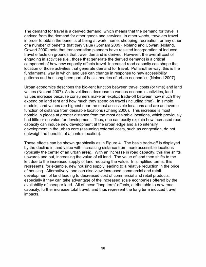
96
The demand for travel is a derived demand, which means that the demand for travel is derived from the demand for other goods and services. In other words, travelers travel in order to obtain the benefits of being at work, home, shopping, recreation, or any other of a number of benefits that they value (Gorham 2009). Noland and Cowart (Noland, Cowart 2000) note that transportation planners have resisted incorporation of induced travel effects on grounds that travel demand is derived. However, the overall cost of engaging in activities (i.e., those that generate the derived demand) is a critical component of how new capacity affects travel. Increased road capacity can shape the location of those activities that generate demand for travel. Put another way, this is the fundamental way in which land use can change in response to new accessibility patterns and has long been part of basic theories of urban economics (Noland 2007). Urban economics describes the bid-rent function between travel costs (or time) and land values (Noland 2007). As travel times decrease to various economic activities, land values increase because consumers make an explicit trade-off between how much they expend on land rent and how much they spend on travel (including time).. In simple models, land values are highest near the most accessible locations and are an inverse function of distance from desirable locations (Chang 2006). This increase is most notable in places at greater distance from the most desirable locations, which previously had little or no value for development. Thus, one can easily explain how increased road capacity can induce new development at the urban edge and also intensify development in the urban core (assuming external costs, such as congestion, do not outweigh the benefits of a central location). These effects can be shown graphically as in Figure 4. The basic trade-off is displayed by the decline in land value with increasing distance from more accessible locations (typically the center of an urban area). With an increase in road capacity, this line shifts upwards and out, increasing the value of all land. The value of land then shifts to the left due to the increased supply of land reducing the value. In simplified terms, this represents, for example, new housing supply leading to a relative reduction in the price of housing. Alternatively, one can also view increased commercial and retail development of land leading to decreased cost of commercial and retail products, especially if they can take advantage of the increased scale economies offered by the availability of cheaper land. All of these “long term” effects, attributable to new road capacity, further increase total travel, and thus represent the long term induced travel impacts.
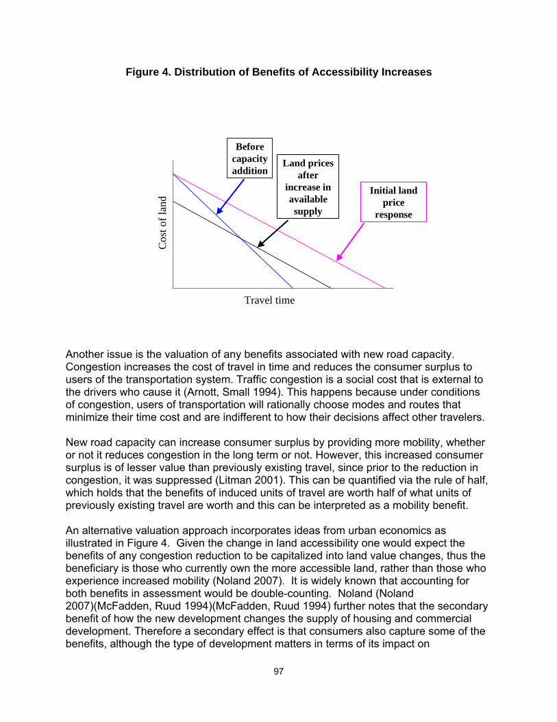
97
Figure 4. Distribution of Benefits of Accessibility Increases
Another issue is the valuation of any benefits associated with new road capacity. Congestion increases the cost of travel in time and reduces the consumer surplus to users of the transportation system. Traffic congestion is a social cost that is external to the drivers who cause it (Arnott, Small 1994). This happens because under conditions of congestion, users of transportation will rationally choose modes and routes that minimize their time cost and are indifferent to how their decisions affect other travelers. New road capacity can increase consumer surplus by providing more mobility, whether or not it reduces congestion in the long term or not. However, this increased consumer surplus is of lesser value than previously existing travel, since prior to the reduction in congestion, it was suppressed (Litman 2001). This can be quantified via the rule of half, which holds that the benefits of induced units of travel are worth half of what units of previously existing travel are worth and this can be interpreted as a mobility benefit. An alternative valuation approach incorporates ideas from urban economics as illustrated in Figure 4. Given the change in land accessibility one would expect the benefits of any congestion reduction to be capitalized into land value changes, thus the beneficiary is those who currently own the more accessible land, rather than those who experience increased mobility (Noland 2007). It is widely known that accounting for both benefits in assessment would be double-counting. Noland (Noland 2007)(McFadden, Ruud 1994)(McFadden, Ruud 1994) further notes that the secondary benefit of how the new development changes the supply of housing and commercial development. Therefore a secondary effect is that consumers also capture some of the benefits, although the type of development matters in terms of its impact on
Cos
t of l
and
Travel time
Before capacity addition
Initial land price
response
Land prices after
increase in available supply

98
environmental costs. A further issue in terms of evaluation of economic effects is the potential to encourage or discourage agglomeration of economic activities. Graham (Graham 2007) suggests that congestion reduction can improve the external productivity gains achievable from firm agglomeration, but does not distinguish road from public transit effects. One additional consequence of building increased highway capacity is that it can undermine existing public transit. Public transit can be efficient in terms of energy consumption and emissions. However, it derives its ability to compete with private vehicle transportation from the frequency with which it can run, and the fares that are charged. The Downs-Thomson paradox addresses the equilibrium between a congested route and public transit. In a hypothetical illustrative case, Arnott and Small (Arnott, Small 1994) describe a train line in which the operator breaks even by only running trains when they are filled to capacity. As a result the frequency of train runs is a function of total ridership, which determines maximum travel time, including waits. If a parallel congested road has its capacity increased, some travelers will shift away from using the train. As riders shift to the competing roadway the train loses ridership and therefore cuts service (or raises fares). This makes the train less competitive, resulting in further shifts to car usage. Eventually the train is shut down as it is no longer competitive. In the end it is shown that congestion is potentially worse on the parallel road than before the capacity increase. In fact price elasticities for transit are fairly small but elasticities for service frequency can be considerably higher (Cervero 1990, Kemp 1973) lending credibility to the Downs-Thomson paradox. Theoretically, we can conclude that one would expect to find that increases in road capacity are likely to increase total travel, especially when projects are aimed at congestion reduction. However, even roads that simply provide greater access under conditions of no congestion may facilitate increased development that leads to increased travel. While the theory is straightforward, empirically estimating this effect can be more problematic. In the next section we review recent research that has examined the empirical evidence for these effects. Some of these approaches might also provide a framework for forecasting future impacts. Empirical Research Evidence and Forecasting Methods
In recent years a number of studies have empirically estimated induced travel, with the aim of demonstrating that a statistically significant relationship can be found between lane miles of road capacity and vehicle miles of travel. These studies typically use aggregate data and multivariate approaches to examine this association. Some go further to examine the endogeneity of traffic growth, that is, whether traffic growth in itself generates the construction of new road facilities. The majority of the empirical analyses has demonstrated that there is a relationship between new roads and extra traffic that is generated, including those analyses that controlled for endogenous effects. We group our discussion to three basic approaches following the classification of Cervero (Cervero 2002). First, we review those studies that used aggregate cross-
99
sectional time-series data for spatial units. Then we discuss those that examined a cross-section of specific facilities, across time. Finally, we discuss approaches that have used regional travel models and integrated land use/transportation models as a tool for forecasting VMT growth associated with changes in road capacity. Aggregate Multivariate Regression Models
The majority of studies in this area have estimated multivariate regression models using area-based aggregations (e.g. state, county, or metro area) of both lane miles and VMT using cross-sectional time-series approaches. Exogenous factors, such as income, fuel prices, and population, are typically controlled for. Thus, travel is compared on the aggregate level of facilities by region, producing a demand elasticity for travel. Regression models typically employ VMT as the dependent variable. VMT provides a continuous variable that captures changes in vehicular travel including travel from new trips, the added distance from longer trips, and route changes, which are generally recognized as increases in travel (Cervero 2002, DeCorla-Souza, Cohen 1998). Barr (Barr 2000) describes VMT as a good summary measure of the number of trips, their spatial distribution, modal choices, and route choices, and a good indicator of energy consumed (and consequent carbon emissions). Although these studies use a direct measure of the dependent variable (Cervero, Hansen 2002, Barr 2000), they do not as directly measure the impact of changes in travel demand on emissions (Rodier et al. 2001), which are generally linked to the flow characteristics of the traffic network as well as the mix of vehicles in the fleet. However, these effects are generally overwhelmed by increased use (Litman 2001, Noland 2007, Noland, Quddus 2006). Because validation of the hypothesis of induced travel is based on analysis of counterfactuals, demonstration of causality is generally based on several factors. In order for changes in highway capacity to be causal to the quantity of travel demanded the following must be demonstrated:
• There must be correlation between highway capacity and vehicular travel; • Changes in highway capacity must precede changes in vehicular travel; • Competing causal factors must be accounted for; • Endogeneity must be properly controlled for.
The latter condition is the most problematic, but has been tackled by several studies. Much of the analysis that has been done uses cross-sectional time-series (panel) data on spatial units of analysis (i.e., counties, urban areas, or states). Dummy variables are generally used to capture fixed effects of sub regions and time periods to factor out those factors associated with a given region or that may change over time.
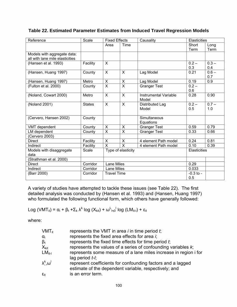
100
Table 22. Estimated Parameter Estimates from Induced Travel Regression Models
Reference Scale Fixed Effects Causality Elasticities Area Time Short
Term Long Term
Models with aggregate data: all with lane mile elasticities
(Hansen et al. 1993) Facility X 0.2 – 0.3
0.3 – 0.4
(Hansen, Huang 1997) County X X Lag Model 0.21 0.6 – 0.7
(Hansen, Huang 1997) Metro X X Lag Model 0.19 0.9 (Fulton et al. 2000) County X X Granger Test 0.2 –
0.6
(Noland, Cowart 2000) Metro X X Instrumental Variable Model
0.28 0.90
(Noland 2001) States X X Distributed Lag Model
0.2 – 0.5
0.7 – 1.0
(Cervero, Hansen 2002) County Simultaneous Equations
VMT dependent County X X Granger Test 0.59 0.79 LM dependent County X X Granger Test 0.33 0.66 (Cervero 2003) Direct Facility X X 4 element Path model 0.24 0.81 Indirect Facility X X 4 element Path model 0.10 0.39 Models with disaggregate data
Scale Type of elasticity Elasticities
(Strathman et al. 2000) Direct Corridor Lane Miles 0.29 Indirect Corridor Lane Miles 0.033 (Barr 2000) Corridor Travel Time -0.3 to -
0.5
A variety of studies have attempted to tackle these issues (see Table 22). The first detailed analysis was conducted by (Hansen et al. 1993) and (Hansen, Huang 1997) who formulated the following functional form, which others have generally followed: Log (VMTit) = αi + βt +Σk λk log (Xkit) + ωL
l=0l log (LMit-l) + εit where: VMTit represents the VMT in area i in time period t;
αi represents the fixed area effects for area i; βt represents the fixed time effects for time period t; Xkit represents the values of a series of confounding variables k;
LMit-l represents some measure of a lane miles increase in region i for lag period t-l;
λk,ωl represent coefficients for confounding factors and a lagged estimate of the dependent variable, respectively; and
εit is an error term.

101
The use of the logarithmic form has two advantatges. First, it minimizes any issues of heteroskedasticity, by reducing that might occur by including regions with large variances in size. Second, it allows one to interpret coefficient estimates as elasticities, although this also assumes that elasticities are constant and independent of the existing level of road capacity. In itself this is not an unrealistic assumption, but also as these studies are mainly concerned with identifying a statistically significant effect, the absolute magnitude of the estimated elasticity is less critical. (Hansen, Huang 1997) estimate travel demand elasticities at the county and metropolitan levels with panel data for 30 urban counties in California, with aggregation assignments to the metropolitan level. (Hansen, Huang 1997) control for area and time fixed effects, population, personal income and fuel price. They report short run elasticities of 0.21 and 0.19 at the county and metropolitan levels respectively and between 0.6 and 0.7 at the county level and 0.9 at the metropolitan level for long run elasticities. (Fulton et al. 2000) estimate county-level travel demand elasticities for three states and Washington, DC with cross sectional time series data. (Fulton et al. 2000) control for area and time fixed effects and population, population density and employment. A growth model is used to correlate VMT growth with increases in lane miles, enabling a Granger causality test to evaluate precedence of the associated increases of VMT with prior increases in capacity, i.e. lane miles. A growth variable for lane miles is used as an instrument in a second stage to address simultaneity bias with one year and two year lag periods. As a result (Fulton et al. 2000) report short term lane mile elasticities between 0.2 and 0.6, the first successful model to establish a causal linkage. (Noland, Cowart 2000) estimate travel demand elasticities for freeways and arterial roads at the metropolitan area level. They use an instrumental variable approach, controlling for fixed effects of area and time, controlling for population density, per capita income, proportion urban area, and fuel costs. (Noland, Cowart 2000) estimate a short term elasticity of 0.28 and a long term elasticity of 0.90, however, the instrument selected was found to be weak, questioning any firm conclusions of a causal effect. (Noland 2001) estimates state level travel demand elasticities with cross sectional time series data, controlling for population, income and fuel cost changes and separately treating facility types based on established road categorization schemes, from rural collector roads to interstate routes. A range of models are estimated including seemingly unrelated regression estimates by road type for short term elasticities, a distributed lag model to estimate long term elasticities, and growth models to address multi-collinearity among the independent variables. As a result travel demand elasticities between 0.2 and 0.5 were estimated for the short term and between 0.7 and 1.0 for the long term. The large variety of models estimated provide a large degree of robustness in the estimates, however none deal explicitly with endogenous effects. (Noland 2001) also produced a short term forecast, of future VMT growth, which might

102
serve as a basis for an aggregate forecast of VMT and carbon emissions using readily available inputs. (Cervero, Hansen 2002) demonstrate the mutual causality of VMT and lane mile expansion. Using simultaneous equations for supply and demand and instrumental variable regressions, that include political variables as instrument, they find a statistically significant induced travel effect. They also find that increases in VMT lead to more road capacity, i.e., that there is a two-way effect confirming the view that planners have some foresight about where road capacity will be demanded. This latter effect, however, is smaller than the estimated coefficient on lane miles, associated with VMT. (Liu et al. 2006) estimate a series of models using county-level data from Pennsylvania. They find very high lane-mile elasticities and significance levels, but likely have major problems with multicollinearity in their data. They claim that their lane-mile elasticities are high because they capture reclassification of various road categories, such as rural to urban. They use their models as a means of forecasting statewide VMT, an approach that might be feasible with these sort of models as a way of estimating carbon emissions. A recent model using data from Switzerland also finds a significant induced travel effect (Weis, Axhausen 2009). Using a pseudo-panel constructed from a series of national travel surveys, an accessibility indicator is constructed as is a generalized cost index. Estimation of a structural equation model shows a statistically significant effect of elasticities for various components of travel demand; for example number of trips, trip distance, and trips per tour are calculated. This is one of the benefits of using this type of data which allows disaggregation of different behavioral components. However, the key conclusion from this study is again that there is a large and statistically significant effect, although it is difficult to strictly compare their elasticities with the other studies listed in Table 22. As Table 22 demonstrates, all of these models find statistically significant effects and parameter estimates within reasonable ranges. (Cervero, Hansen 2002) and (Cervero 2003) note that all these models used similar methodologies, and suggest that different approaches are needed to more firmly establish the validity of the theoretical effects. Facility-Specific Studies
Facility-specific studies have examined the impact of specific links or corridors within the transportation network and subsequent growth in VMT. These include growth comparisons and quasi-experimental or matched-pair comparisons. Regression models have also been employed using facility level data as an independent variable. A matched pair study, conducted by (Mokhtarian et al. 2002) was conducted using California data. This study attempted to match similar roads, with and without a capacity improvement, and confounders were assumed to be controlled for by matching similar road pairs. This type of study would not be able to control for endogeneity, in

103
that a transportation planning authority made a presumably rational choice to improve one facility but not its comparable mate in a matched pair. Likewise, any network effects associated with the improved road, such as growth on alternative routes, would not be properly captured. It is unsurprising, therefore, that (Mokhtarian et al. 2002) found no significant effect. (Goodwin 1996) reviewed facility-specific studies (mainly bypasses of town centers in the United Kingdom) connecting distance traveled to fuel cost, highway capacity, and travel time. He found fuel cost elasticities within a range of -0.1 to -0.5. That review estimated an elasticity of traffic relative to highway capacity of 0.11, which approximated a benchmark. (Goodwin 1996) estimated the elasticity of demand for time based on a cross elasticity for the demand for money, particularly as fuel cost as follows: Et = Em * Vt * M where Et is the demand elasticity for time savings, Em is the demand elasticity for fuel cost savings, Vt is the value placed on time and M is the money value of fuel cost (p.40). This provides a basis from which (Goodwin 1996) calculates demand elasticities with respect to travel time. On this basis generalized observed traffic flows between 10% and 20% higher than a null hypothesis of no induced traffic, with a range between 0% and 40% are predicted. What was found was an average increase of 20% within a range of 9% to 44% of the flow before improvements. Long term increases were even higher. (Goodwin 1996) also noted that growth of peak period flows were relatively higher, suggesting that peak-spreading was diminished, while some alternate routes had lower flow than predicted. (Goodwin 1996) approximated an average travel time elasticity of -0.5 in the short run and -1.0 in the long run based on the literature at that time. (Cervero 2003) estimates a structured equation model that includes changes in road speed, as the mediating influence on behavioral change, and links new capacity to development activity and VMT. His estimates also account for endogenous effects of how VMT and development activity affect both speeds and increased road capacity. Road capacity is measured using a selection of specific projects, rather than aggregate changes in lane miles as other models have done. He finds statistically significant effects and this suggests a useful approach for linking individual projects to potential increases in carbon emissions. Cervero’s results are listed in Table 22 and provide both short and long run elasticity estimates. While he claims that he shows smaller effects than other studies, this is not an accurate interpretation of other results. He attributes about 40% of VMT growth to capacity improvements, while (Noland 2001) found at most 28%, with other demographic and economic factors associated with the remainder. Despite this flaw in how Cervero’s model results have been interpreted, the structure is useful for dissecting different sources of growth in VMT (speeds and development effects) and for accounting for endogeneity. (Cervero 2003) suggests that more sophisticated modeling of travel demand may result in lower elasticity estimates, which could most usefully be used to calibrate long range travel forecasting and urban simulation models such as MEPLAN, TRANUS, and

104
TRANSIMS. Like (Gorham 2009), (Cervero 2003) is concerned with accuracy of measurement. However, Cervero’s (Cervero 2003) concern is more with over than underestimation, because he perceives a political agenda and methodological sloppiness have exaggerated estimates to the detriment of those interests served by development. We discuss these more disaggregate approaches using integrated transport and land use models in the next section. Disaggregate Data Analysis
(Strathman et al. 2000)(Williams 1977)(Williams 1977) use panel data to estimate a model for 48 urban areas in the United States for the purpose of distinguishing between the direct effects of highway capacity measured as lane miles and the indirect effects factoring out the effects on residential and employment location choices of lane miles on VMT. They select a sample of roughly 12,000 individual respondents from the 1995 Nationwide Personal Transportation Survey (NPTS) and 48 urban areas from the Texas Transportation Institute database. (Strathman et al. 2000) report a direct elasticity of per capita roadway capacity to VMT of 0.29 and an indirect elasticity (representing the secondary effects due to changes in land use) of 0.033. The meaning of the indirect elasticity value is questionable because residential and employment location choices are affected by induced travel effects. It is doubtful that the indirect elasticity would be much help in estimating future effects. (Barr 2000) also used the NPTS data to estimate short term elasticities. However, his sample was nationwide and included roughly 27,000 households of which 61% were in urbanized areas and 63% had access to public transportation. A model was estimated with VMT as the dependent variable while the independent variables included the inverse of speed, census tract population density, annual and per capita family income, household size, number of workers in households, the median household income of the census tract and an error term. (Barr 2000) estimates travel time elasticities between -0.3 and -0.5. It is notable that models using both aggregate and disaggregate data, estimated at a variety of levels of spatial aggregation, predict travel demand elasticities in a range of about 0.2 to 0.6 in the short term and 0.6 to 1.0 in the long term. These results show stability in the reliability of travel demand elasticities in that they can be arrived at consistently by more than one method. It is pointed out broadly that the fact of a correlation does not imply causality on the face of it (Noland, Lem 2002, Cervero 2002). The direct lane mile elasticities calculated using both methods appear comparable in magnitude. Although the range of elasticities seems somewhat larger in the aggregate regression models, the small number of studies, the variety of models, and the differences of geographic scale and facility type may have contributed to this. It is not possible to assess what loss of effectiveness there is in choosing a direct measure of the dependent variable, i.e. travel time, over a proxy measure, i.e. lane miles, although the results seem to show considerable consistency.

105
Disaggregate Regional Travel Demand Models and Land Use Modeling
(Cervero 2002) and (Noland, Lem 2002) note that among transportation planners there is a preference for disaggregate models, as opposed to the aggregate regression models previously discussed. This largely dates to problems with zonal gravity model approaches used in the early years of transportation planning, but disaggregate individual level modeling comes with its own costs and complexities, especially for estimating induced travel effects. Several methods have been used, including the use of four-step travel demand modeling approaches.
Table 23. Estimates using travel demand models.
Model Method Scale Type Elasticities Short
Term Long Term
(DeCorla-Souza 2000) No Feedback Four step Facility Travel Time -0.7 * Feedback Four step Facility Travel Time -1.1 * (Rodier et al. 2001) 25 years MEPLAN Metro Lane Miles 0.8 50 years MEPLAN Metro Lane Miles 1.1 * Term uncertain. Four step models are the traditional approach to estimating travel demand used to assess specific road and transit projects. Four step models are generally zonal in nature, although there are disaggregate modeling applications that address travel behavior at the person or household level (Frank, Stone 2000). In practice, they generally lack sufficient feedback mechanisms and are widely acknowledged to fail to fully capture induced travel effects. Some areas have implemented more complex activity-based modeling approaches that might better capture some of these effects, but may still not adequately account for the multitude of feedback mechanisms required for a full accounting, in particular feedback to land development effects. Four step models are able to directly calculate time elasticities (DeCorla-Souza 2000) (McDonald 2008)(McDonald 2008)or lane mile elasticities (Rodier et al. 2001). (Rodier et al. 2001) implement the MEPLAN integrated land use/transport model for metropolitan Sacramento to explicitly examine induced travel effects. MEPLAN, in theory, allows for the full integration of land use and economic effects associated with lane mile increases, as opposed to the typical exogenous assumptions made on how land use may change. They find significant differences associated with forecasts that assume induced travel effects compared to not using sufficient feedback (Rodier et al. 2001) estimate forecasts for 25 and 50 year predictions and assess the sensitivity of criteria pollutants to the corrections of their enhancements by withholding the effects of the enhancements that would not be found in a traditional four step model. At 25 years they project the following differences in increases of emissions between their model and a hypothetical traditional four step model: total organic gases (TOG) 10% vs. -5%, Carbon Monoxide (CO) 12% vs. -2%, Nitrogen Oxides (NOx) 12% vs. -1%, and

106
particulate matter (PM) 8% vs. -8%. At 50 years they project the following differences between their model and a hypothetical model: TOG 9% vs. -7%, CO 13% vs. -4%, NOx 16% vs. -1%, and PM 6% vs. -9%. For every pollutant the traditional model predicted a decrease while induced travel effects suggest a substantial increase. They do not include an estimate for CO2 emissions, but that can easily be done with this sort of approach. The MEPLAN modeling framework that (Rodier et al. 2001) includes separate but interactive land and transportation markets. The region is disaggregated spatially and classified by land use type. Discrete choice models predict the location choices based on the attractiveness of each, which is a function of activity-specific input costs including transportation costs based on a transportation network and location-specific disutilities. Through an incremental model, lags provide feedback of transportation costs from one period to the land market model of the next, so that land use is handled dynamically. This application includes eleven industry classifications to match employment with locations; three classifications of household income that incorporates residential location; business consumption of household labor; business activities of households to purchase goods and services; and, consumption of space based on elasticities for seven types of land use. Vacant land and different rents paid for similar land use are also tracked. Exogenous demand by industry and retiring and unemployed households is accounted for. In addition to the land use components, they also made substantial improvements to the Sacramento regional transportation model, to better incorporate other induced travel effects (beyond the long term land use impacts). These specifically include better feedback from trip generation, distribution, mode choice, and network assignment steps of the model. (Rodier et al. 2001) report lane mile elasticities of 0.8 projected out 25 years and 1.1 projected out 50 years. Using a simpler model without the intricate feedbacks of (Rodier et al. 2001), (DeCorla-Souza 2000) reports travel time elasticities of -0.7 with feedback withheld and -1.1 with feedback accounted for. (DeCorla-Souza 2000) does not state the time frame in connection with these travel time elasticities, although he notes that they are above a benchmark of -0.4 which represents the average long term household travel time elasticity for personal highway travel. (Dowling et al. 2005) attempted to develop a full model for estimating how a specific project may induce travel and link this to the emissions from vehicles. This project included a modal emissions model to account for how vehicle dynamics change in response a given project. While this is a useful approach to follow, the main problem with their approach is the large amount of error introduced by any large scale modeling effort. In theory, this would be a problem with any regional travel demand model, including the integrated approach used by (Rodier et al. 2001). Other approaches include those of (Waddell et al. 2007) that implement the UrbanSim location choice model. These types of land use models are dependent on large databases disaggregated to parcel level data and are estimated using discrete choice methods,

107
which can introduce significant levels of uncertainty and error in the results. As an example of the inherent uncertainty of all these approaches, (Rodier, Johnston 2002) found emissions forecasting to be very sensitive to population and employment growth such that it would likely swamp any measurable impact from a specific project, using regional modeling approaches. Sketch Planning Models
The FHWA has developed at least two simple sketch planning models that presumably account for induced travel effects. These are the SMITE and STEAM models. SMITE was developed as a method to estimate induced travel effects at the corridor level. SMITE uses travel time elasticities, based on (Goodwin 1996) to estimate trips that are diverted to an improved facility. This is represented by Vi = Ho / (M – (Ed * Sav)), where Vi is induced VMT, Ho is the initial time savings from an investment, M is the increase in drive time for other drivers due to congestion per added vehicle, Ed is the elasticity of the demand for time, and Sav is the average speed, (DeCorla-Souza, Cohen 2009) (p. 5). The increase in travel time (Hi) is based on the induced VMT and the initial congestion level: Hi = Vi * M so that Vi = Hi / M. Because Ed is negative and average speed is positive, the congestion term in the denominator after the induced effects set in is M – (Ed * Sav) and should be greater than the initial congestion term M. Users input initial conditions on the freeway and the arterials including initial VMT, and the proportional freeway and arterial shares of VMT. SMITE calculates initial, arterial and freeway VMT and diverted and induced VMT for the arterials, the freeway, and the corridor as a whole, for low, moderate, and high congestion levels. SMITE also calculates changes in average speed based on the improvement, and thus potentially offers a way to calculate emissions. STEAM is the second generation of sketch planning tool designed by FHWA for the purpose of conducting cost benefit analysis on transportation planning alternatives at the corridor level (DeCorla-Souza, Hunt 1999). It replaces SPASM, a spreadsheet application. STEAM performs cost benefit analyses, including assessment of global warming impacts based on CO2 emissions, as well as criteria pollutants: HC, CO, NOx, and PM. STEAM improves on SPASM, its predecessor, by addressing VMT rather than volume measurements. It accepts output from four-step modeling applications after the traffic assignment step. It can accommodate travel demand forecasts but does not incorporate induced travel effects. STEAM has four components including a user interface and a network analysis model, which holds the parameters of a traffic grid including highway traffic volumes, the lengths, capacities, and related information about facility links, including distance based on minimized time costs (DeCorla-Souza, Hunt 1999). Another component implements trip table analysis and estimates costs and benefits through comparison of base and improved case scenarios, including emissions. The fourth component provides a summary. STEAM handles multiple modes including private auto, carpool, bus, walking to light rail, and driving to light rail for home-based purposes including work, school, non-work, as well as non home-based trips and truck travel. Motor vehicle speed is

108
calculated based on average weekday traffic-to-capacity ratios (AWDTC) (DeCorla-Souza, Hunt 1999), p.6). Non-highway passenger travel is based on passenger count data. STEAM uses a trip based approach to estimate emissions, by which for each trip the emissions based on hot-stabilized VMT is added to the increased emissions that result from a cold start, i.e. the difference between start and hot-stabilized emissions for a proportion of all trips. That proportion has a default but is adjustable. CO2 and other greenhouse gas emission estimates are based on fuel consumption (DeCorla-Souza, Hunt 1999)(Guo, Bhat & Copperman 2007)(Guo, Bhat & Copperman 2007). While this model has significant detail, it is not designed to explicitly examine the effects associated with induced travel. Forecasting and Estimating CO2 Emissions
The key objective here is to determine whether any of these approaches can provide a simple and valid means of estimating project specific CO2 emissions. While integrated land use / transportation models offer a very detailed method, they suffer from significant potential errors that make assessment of emissions associated with a single project (within a large region) prone to being drowned out by other regional impacts (this was a problem with (Dowling et al. 2005). (Rodier et al. 2001) manage to develop estimates, but these are typically for a package of lane mile additions throughout a region. Aggregate econometric methods offer some potential as being a simplified method for estimating CO2 emissions. (Noland 2001) demonstrated this in his state-level study, providing a short term forecast of VMT growth and the effect on CO2 emissions. (Liu et al. 2006) attempt a similar approach using county-level data for Pennsylvania, but do not calculate emissions. Both (Noland 2001) and (Liu et al. 2006) are based on state and county level aggregations, respectively, which do not necessarily translate to a project level assessment. However, the elasticities generated from these studies (or a similar study for New Jersey) can provide a means for estimating increases in facility specific VMT associated with changes in lane miles. The method developed by (Cervero 2003) provides one option for using facility-specific lane mile changes to estimate VMT growth. Data necessary to estimate these models is typically readily available or can be supplied by DOT. In addition to data on VMT and lane miles (perhaps disaggregated to facility type), various demographic and income data is also used, as well as fuel prices. Much of the demographic data is highly correlated, so in practice it is often impossible to use more than total population and income within most models. The advantage of these approaches is the simplicity of the data inputs and the clarity of the models; as opposed to large scale regional models which have many uncertainties. The key benefit of these approaches is nicely summed up by (Goodwin 1992) who said: “demand elasticities are, in general, rather crude and approximate measures of aggregate responses in a market. They do, however, have the great attractions of being empirically estimable, reasonably easily understood, tested by experience, and directly

109
usable for policy assessment. (p. 155)” They are desirable planning tools because they show relationships in a way that is useful for prediction. While these methods offer an approach for estimating VMT growth, conversion to CO2 emissions potentially adds additional complexity. The fuel efficiency of the vehicle is directly linked to CO2 emissions, for a given fuel type. Most vehicles use gasoline, frequently with a 10% ethanol blend. Diesel vehicles tend to be more fuel efficient, but represent a relatively small share of personal vehicles. Emissions estimation models, specifically those developed by EPA (the Mobile6 model and the soon to be released MOVES model) account for the characteristics of the vehicles in the fleet in calculating emissions. The Mobile6 model separates the driving process into three stages, including cold starts in which engines run inefficiently until they become hot-stabilized and operate at peak efficiency, warm starts, and hot-stabilized, with separate profiles for each (Barth et al. 1996)(Barth et al. 1996, Frank et al. 2007)(Barth et al. 1996, Frank et al. 2007). Emissions are estimated based on average speeds and distance traveled. Adjustments are made to correct for fuel type, ambient temperature, and acceleration/deceleration, but the effects of acceleration and deceleration are underestimated (Barth et al. 1996). Thus a key deficiency of these models is that they do not adequately account for how changes in the road network may change the dynamics of vehicle acceleration and the levels of stop and go driving, both of which tend to lead to reduced vehicle efficiency and consequently more CO2 emissions. Several approaches have been developed to better estimate the microscopic emissions associated with vehicle operation. These include the Comprehensive Modal Emissions Model (CMEM) developed at the University of California, Riverside (Barth et al. 1999). This model provides a method to link second-by-second operation of the vehicle to instantaneous emissions. In practice these can be integrated with a microscopic traffic simulation model (e.g. VISSIM, Paramics, Transims). This has been done by (Stathopoulos, Noland 2003) and (Noland, Quddus 2006) to specifically examine how much induced travel negates the short-term emissions reductions from congestion reduction projects. In the short term, these models demonstrate how reducing stop-and-go traffic, excess idling, and hard accelerations will reduce vehicle emissions (especially criteria pollutants). This effect is demonstrated in both studies. These studies then assume various levels of induced travel, which in theory would occur in response to a congestion reduction, and find that emissions tend to rapidly increase to initial levels. While there is variation based on the assumptions used, in general, the levels of traffic generated that negate the emissions benefit are well within the expected range suggested by induced travel studies. This effect tends to be larger for criteria pollutants than for CO2 emissions, but it still occurs in most instances for the latter. (Noland, Quddus 2006) further show that as vehicle technology has improved, the short term improvements have diminished, implying a greater correlation between VMT and emissions, as opposed to the effects from accelerations and stop-and-go driving conditions. New hybrid vehicles tend to also be more efficient
110
in urban driving conditions than in free-flow high-speed conditions; primarily due to the ability to rely on battery power at lower speeds. The CMEM model is relatively dated and was based on a limited dataset of vehicle, and thus is not appropriate for actual measurement. The overall technique of simulated back-casting of induced travel impacts, however, offers a simple approach for evaluating CO2 emissions, without explicitly specifying any demand model. This method could be used with the new MOVES model combined with a traffic micro-simulation. The MOVES model (released in Jan 2009) will estimate the full range of GHG emissions. In addition to CO2 this includes nitrous oxide (N2O), and methane (CH4) (Koupal et al. 2002). MOVES will allow classification of separate classes of motor vehicles and off-road equipment. It will allow estimation based on operating mode bins that capture discrete operating modes of vehicles. Operating modes for motor vehicles include cold and warm starts and hot-stabilized running as with MOBILE, but have been expanded to handle extended idling, upstream energy use associated with fuel use by a source, and emissions associated with manufacture and disposal. The intent is to capture full life cycle emissions. MOVES is designed to handle combustion emissions from running and start exhaust, and extended idle, hydrocarbon emissions from hot soak, diurnal, resting loss, as well as running and refueling loss. It is also designed to handle effects from brake and tire wear. Analysis can be done at a high level of aggregation or macroscale, which is a county level analysis, a mesoscale, which is appropriate for local analyses and is at the facility link level of resolution, or at a microscale for estimating emissions in specific corridors or facilities. These levels have decreasing time resolutions as well. MOVES incorporates a four step procedure and a set of utilities referred to as data generators that are essentially after processors (Koupal et al. 2002). Currently, the MOVES model does not include sufficient detail on the characteristics of hybrid vehicles and thus this limits the ability to consider the interaction of new technologies with flow improvement projects. However, eventually the vehicle database will presumably include this capability. Conclusions
This review has focused on establishing the basic theoretical features of how traffic is induced in response to new road capacity. Basic economic theory provides a fundamental relationship between road supply and demand with travel time of individuals being the price that is determined at equilibrium. We further show how basic urban economic theory implies that long-run effects can be captured by changes in land use and consequently new development that occurs in response to increased accessibility. Thus this leads us to conclude that theoretically there is no question of how reducing congestion through new road projects, or even building new roads that access undeveloped land, will result in increased vehicle travel. Our review of empirical studies finds conclusive evidence of this theoretical relationship. We also examined whether any of the empirical methods might be suitable for

111
forecasting and estimates of CO2 emissions. Some models have been used for this purpose and in theory a model could be developed for New Jersey with suitable data. These can use either county-level aggregations of changes in road capacity, or even facility-level changes, if a suitable time-series is available. The key uncertainty is how forecasts of population, income, and fuel prices may affect future VMT, but for a comparative analysis, one can examine alternative scenarios. The other approach frequently advocated is the use of integrated transport/land use models. These tend to be very data intensive, and while some models are based on a strong theoretical basis, the implementation is both difficult, costly, and potentially prone to error, especially if examining the impacts from only one project. Calculating emissions from VMT will ultimately be done with the MOVES model set to be released by EPA in January 2009. This model is being developed such that facility-specific impacts can be evaluated. The model can also be integrated with a traffic microsimulation model. This latter approach provides a way to evaluate the changes in vehicle dynamics and the details of how vehicle flow may change. While MOVES does not provide second-by-second emissions, as do experimental models such as CMEM, it is an improvement over Mobile6. Back-casting approaches can then be used to examine different assumptions on how traffic levels may grow in response to specific changes in the traffic network.

112
CONCLUSIONS AND FURTHER RESEARCH NEEDS
This report documents the development of the GASCAP spreadsheet software for analyzing the life-cycle greenhouse gas emissions from transportation capital projects. Over the course of this project we have identified additional research needs and further work to fully develop this as a tool that NJDOT can use to assess and compare different projects. Each of these key areas is outlined below. Materials module
The current materials module is based on over 1000 bid-sheet items plus detailed calculations for asphalt and concrete, allowing variations in production processes to be modeled. Despite this, our case studies found various gaps in our coverage of bid sheet items. Feedback from NJDOT staff is necessary on this module to help find missing components. In addition, various electronic and landscaping items (700 and 800s in the bid-sheets) were not included but could be added with additional effort. Other minor materials could also be included. Equipment module
The main shortcoming of GASCAP is that it is necessary for users to use informed judgment about the mix of equipment and the duration of its use for each project. There is no current information on equipment activity for specific projects. While we expect that contractors and NJDOT engineers likely can assess these needs, ideally the data should be compiled and connected with specific project types, particularly those that occur on a frequent basis. Information on fuel consumption associated with a sample of projects may allow us to develop models that estimate fuel consumption for projects and allow us to allocate these to equipment. Another project currently being completed by a NJDOT contractor should be available in August 2011 and will provide a starting point for this analysis (see also discussion under life-cycle maintenance). Life-cycle maintenance
An original objective was to develop an approach that could evaluate how maintenance over the life of a project could reduce overall greenhouse gas emissions. Unfortunately we were unable to find standard procedures or reports that document best practices used by NJDOT. We were able to find some reports from other states and the current software contains an uncompleted module that lays out a framework for a life-cycle maintenance approach. This was not completed, as a critical input was to coordinate this component with another project being completed by a NJDOT contract that is not expected to be ready until August 2011. When this data is available, it should provide an opportunity to estimate fuel consumption for a variety of maintenance activities with some additional effort applying the NONROAD model. These data could also be used to estimate GHG emissions from construction activities.

113
Once this module is completed, it will be incumbent upon NJDOT staff to provide feedback so that the defined maintenance procedures are compatible with NJDOT practice. Staging module
GASCAP currently includes a module that allows the user to input information on how the project will be staged. This module could be significantly upgraded by providing estimates of how traffic is delayed or diverted during road closures. Estimates of the increase in GHG emissions from this traffic would be beneficial for making decisions on how best to stage a project to minimize GHG emissions. This will also require a more detailed mapping algorithm for calculating alternative routes, than is currently used by GASCAP for estimating transportation distances for project materials to the site. Lighting module
Additional lighting technologies are rapidly coming on line. We will need to update the available technologies in the lighting (and staging) modules of GASCAP. Rail module
The approach used in GASCAP to estimate rail construction emissions is somewhat limited using average emission estimates based on a small sample of studies, especially for station and platform construction, bridges, and tunneling. This could be improved, pending data availability, by a bottom-up approach that decomposes the individual components in rail construction projects. NJ Transit bid-sheet data is very limited and further work would need to include additional input from NJ Transit on the detailed inputs to their capital projects. Emissions coverage
GASCAP currently does not include estimates for SF6 a GHG which is associated with production of electrical equipment. GASCAP could also be upgraded to include estimates of other criteria pollutants (NOX, VOC, and particulates) allowing it to be used for assessing localized pollutant impacts. Updating procedures
Research into life-cycle GHG emissions is continually evolving, as technology changes and as new information is obtained. For example, recent evidence suggests that natural gas usage may have larger life-cycle emissions than previously thought due to leakage from shale formations currently being exploited. EPA and ANL are continually providing updates to their models (NONROAD, MOVES, and GREET). As a result, procedures are needed to allow the user to easily update GASCAP with inputs from these models for future years.

114
Future technologies
Various future technologies can be investigated for their practical feasibility and to provide options for evaluating them in GASCAP. For example, various “green” pavements, including those with increased reflectivity (see Appendix D) might be feasible to use. Other technologies on the horizon include concrete that is able to absorb greater quantities of CO2. Further discussion with NJDOT staff as to the applicability of these technologies in New Jersey is warranted and consideration of ways to implement these in GASCAP could be analyzed. Induced travel module
DEP staff have expressed a desire for a method that can evaluate the impact of alternative projects on travel behavior. This is a useful endeavor and as part of this project we have provided a review of potential approaches to develop sketch-planning methods that would be able to estimate induced travel and the emissions associated with it. This would be a larger undertaking requiring extensive data collection, and would require significant resources to fully implement. Training, testing and feedback
NJDOT and NJ Transit staff need to be trained on the use of GASCAP. As developed, the software is very user friendly, so we do not anticipate that training is a major task. However, obtaining feedback from staff after they have tested the capabilities of GASCAP is essential. We expect that this will provide useful information on the usability of the software and any major omissions or assumptions that need to be corrected.

115
APPENDIX A. SPARK IGNITION ENGINES
Table 24. Steady State Emissions from Spark Ignition Engines
Emissions and BSFC for Class III Handheld Small Spark Ignition Engines (< 20cc) Engine Tech Type Steady State
HP Min HP Max HC CO NOx PM BSFC
hp-hr hp-hr g/hp-hr g/hp-hr g/hp-hr
g/hp-hr
lb/hp-hr
G2H3 (gas 2-stroke handheld Class III baseline) 0 1 261.000 718.870 0.970 7.700 1.365 G2H31 (Phase 1) 0 1 219.990 480.310 0.780 7.700 1.184 G2H3C1 (Phase 1 with catalyst) 0 1 219.990 480.310 0.780 7.700 1.184 G2H32 (Phase 2) 0 1 33.070 283.370 0.910 7.700 0.822 G2H3C2 (Phase 2 with catalysts) 0 1 26.870 141.690 1.490 7.700 0.822
Emissions and BSFC for Class IV Handheld Small Spark Ignition Engines ($20cc and <50cc) Engine Tech Type Steady State
HP Min HP Max HC CO NOx PM BSFC
hp-hr hp-hr g/hp-hr g/hp-hr g/hp-hr
g/hp-hr
lb/hp-hr
G2H4 (gas 2-stroke handheld Class IV baseline) 1 3 261.000 718.870 0.940 7.700 1.365 G2H41 (Phase 1) 1 3 179.720 407.380 0.510 7.700 1.184 G2H4C1 (Phase 1 with catalyst) 1 3 179.720 407.380 0.510 7.700 1.184 G4H41 (Phase 1 4-stroke) 1 3 22.370 533.420 1.790 0.060 0.847 G2H42 (Phase 2) 1 3 33.070 283.370 0.910 7.700 0.822 G2H4C2 (Phase 2 with catalysts) 1 3 26.870 141.690 1.490 7.700 0.822 G4H42 (Phase 2 4-stroke) 1 3 25.830 432.510 1.130 0.060 0.847
Emissions and BSFCs for Class V Handheld Small Spark Ignition Engines (>50cc) Engine Tech Type Steady State
HP Min HP Max HC CO NOx PM BSFC
hp-hr hp-hr g/hp-hr g/hp-hr g/hp-hr
g/hp-hr
lb/hp-hr
G2H5 (gas 2-stroke handheld Class V baseline) 3 6 159.580 519.020 0.970 7.700 0.921 G2H51 (Phase 1) 3 6 120.060 351.020 1.820 7.700 0.870 G2H5C1 (Phase 1 with catalyst) 3 6 120.060 351.020 1.820 7.700 0.870 G2H52 (Phase 2) 3 6 47.980 283.370 0.910 7.700 0.608 G2H5C2 (Phase 2 with catalysts) 3 6 40.150 141.690 1.490 7.700 0.608

116
Table 22. Steady State Emissions from Spark Ignition Engines – continued
Emissions and BSFCs for Class I Nonhandheld Small Spark Ignition Engines (< 225cc) Engine Tech Type Steady State
HP Min HP Max HC CO NOx PM BSFC hp-hr hp-hr g/hp-hr g/hp-hr g/hp-hr g/hp-hr lb/hp-hr
G2N1 (gas 2-stroke nonhandheld Class I baseline) 3 6 207.9200 485.8100 0.2900 7.7000 0.870 G4N1S (gas side-valved 4-stroke nonhandheld Class I baseline) 3 6 38.9900 430.8400 2.0000 0.0600 1.365 G4N1O (gas overhead-valved 4-stroke nonhandheld Class I baseline) 3 6 13.390 408.840 1.800 0.060 0.991 G2N11 (2-stroke Phase 1) 3 6 120.060 449.660 4.000 7.700 0.870 G4N1S1 (Phase 1 side-valved 4-stroke) 3 6 8.400 353.690 3.600 0.060 0.921 G4N1O1 (Phase 1 overhead valved 4-stroke) 3 6 8.400 351.160 3.240 0.060 0.781 G4N1SC1 (Phase 1 side-valved 4-stroke with catalyst) 3 6 8.400 353.690 3.600 0.060 0.921 G4N1S2 (Phase 2 side-valved) 3 6 7.930 353.690 2.370 0.060 0.921 G4N1O2 (Phase 2 overhead valved) 3 6 6.130 351.160 1.830 0.060 0.781 Emissions and BSFC for Class II Nonhandheld Small Spark Ignition Engines (≥ 225cc) Engine Tech Type Steady State
HP Min HP Max HC CO NOx PM BSFC hp-hr hp-hr g/hp-hr g/hp-hr g/hp-hr g/hp-hr lb/hp-hr
G2N2 (gas 2-stroke nonhandheld Class II baseline) 6 25 207.920 485.810 0.290 7.700 0.870 G4N2S (gas side-valved 4-stroke nonhandheld Class II baseline) 6 25 9.660 430.840 2.060 0.060 0.937 G4N2O (gas overhead-valved 4-stroke nonhandheld Class II baseline) 6 25 5.200 408.840 3.500 0.060 0.937 G4N2S1 (Phase 1 side-valved 4-stroke) 6 25 5.500 387.020 4.500 0.060 0.868 G4N2O1 (Phase 1 overhead valved 4-stroke) 6 25 5.200 352.570 3.500 0.060 0.740 G4N2S2 (Phase 2 side-valved) 6 25 5.500 387.020 4.500 0.060 0.868 G4N2O2 (Phase 2 overhead valved) 6 25 4.160 352.570 2.770 0.060 0.740
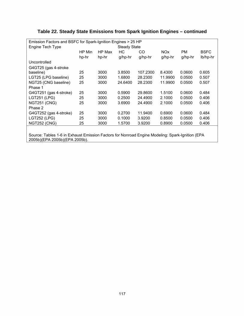
117
Table 22. Steady State Emissions from Spark Ignition Engines – continued Emission Factors and BSFC for Spark-Ignition Engines > 25 HP Engine Tech Type Steady State
HP Min HP Max HC CO NOx PM BSFC hp-hr hp-hr g/hp-hr g/hp-hr g/hp-hr g/hp-hr lb/hp-hr
Uncontrolled G4GT25 (gas 4-stroke baseline) 25 3000 3.8500 107.2300 8.4300 0.0600 0.605 LGT25 (LPG baseline) 25 3000 1.6800 28.2300 11.9900 0.0500 0.507 NGT25 (CNG baseline) 25 3000 24.6400 28.2300 11.9900 0.0500 0.507 Phase 1 G4GT251 (gas 4-stroke) 25 3000 0.5900 29.8600 1.5100 0.0600 0.484 LGT251 (LPG) 25 3000 0.2500 24.4900 2.1000 0.0500 0.406 NGT251 (CNG) 25 3000 3.6900 24.4900 2.1000 0.0500 0.406 Phase 2 G4GT252 (gas 4-stroke) 25 3000 0.2700 11.9400 0.6900 0.0600 0.484 LGT252 (LPG) 25 3000 0.1000 3.9200 0.8500 0.0500 0.406 NGT252 (CNG) 25 3000 1.5700 3.9200 0.8900 0.0500 0.406
Source: Tables 1-6 in Exhaust Emission Factors for Nonroad Engine Modeling: Spark-Ignition (EPA 2005b)(EPA 2005b)(EPA 2005b).
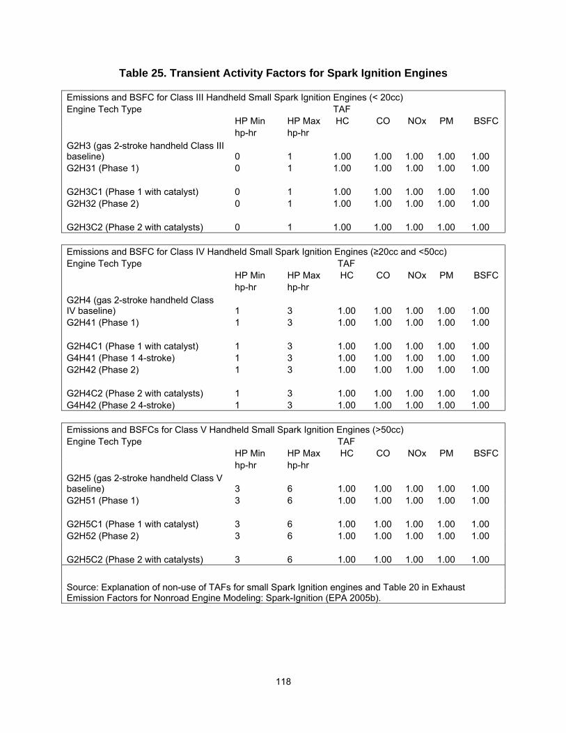
118
Table 25. Transient Activity Factors for Spark Ignition Engines
Emissions and BSFC for Class III Handheld Small Spark Ignition Engines (< 20cc) Engine Tech Type TAF
HP Min HP Max HC CO NOx PM BSFC hp-hr hp-hr
G2H3 (gas 2-stroke handheld Class III baseline) 0 1 1.00 1.00 1.00 1.00 1.00 G2H31 (Phase 1) 0 1 1.00 1.00 1.00 1.00 1.00
G2H3C1 (Phase 1 with catalyst) 0 1 1.00 1.00 1.00 1.00 1.00 G2H32 (Phase 2) 0 1 1.00 1.00 1.00 1.00 1.00
G2H3C2 (Phase 2 with catalysts) 0 1 1.00 1.00 1.00 1.00 1.00
Emissions and BSFC for Class IV Handheld Small Spark Ignition Engines (≥20cc and <50cc) Engine Tech Type TAF
HP Min HP Max HC CO NOx PM BSFC hp-hr hp-hr
G2H4 (gas 2-stroke handheld Class IV baseline) 1 3 1.00 1.00 1.00 1.00 1.00 G2H41 (Phase 1) 1 3 1.00 1.00 1.00 1.00 1.00
G2H4C1 (Phase 1 with catalyst) 1 3 1.00 1.00 1.00 1.00 1.00 G4H41 (Phase 1 4-stroke) 1 3 1.00 1.00 1.00 1.00 1.00 G2H42 (Phase 2) 1 3 1.00 1.00 1.00 1.00 1.00
G2H4C2 (Phase 2 with catalysts) 1 3 1.00 1.00 1.00 1.00 1.00 G4H42 (Phase 2 4-stroke) 1 3 1.00 1.00 1.00 1.00 1.00
Emissions and BSFCs for Class V Handheld Small Spark Ignition Engines (>50cc) Engine Tech Type TAF
HP Min HP Max HC CO NOx PM BSFC hp-hr hp-hr
G2H5 (gas 2-stroke handheld Class V baseline) 3 6 1.00 1.00 1.00 1.00 1.00 G2H51 (Phase 1) 3 6 1.00 1.00 1.00 1.00 1.00
G2H5C1 (Phase 1 with catalyst) 3 6 1.00 1.00 1.00 1.00 1.00 G2H52 (Phase 2) 3 6 1.00 1.00 1.00 1.00 1.00
G2H5C2 (Phase 2 with catalysts) 3 6 1.00 1.00 1.00 1.00 1.00
Source: Explanation of non-use of TAFs for small Spark Ignition engines and Table 20 in Exhaust Emission Factors for Nonroad Engine Modeling: Spark-Ignition (EPA 2005b).

119
Table 23. Transient Activity Factors for Spark Ignition Engines – continued. Emissions and BSFCs for Class I Nonhandheld Small Spark Ignition Engines (< 225cc) Engine Tech Type TAF
HP Min HP Max HC CO NOx PM BSFC
hp-hr hp-hr G2N1 (gas 2-stroke nonhandheld Class I baseline) 3 6 1.00 1.00 1.00 1.00 1.00
G4N1S (gas side-valved 4-stroke nonhandheld Class I baseline) 3 6 1.00 1.00 1.00 1.00 1.00 G4N1O (gas overhead-valved 4-stroke nonhandheld Class I baseline) 3 6 1.00 1.00 1.00 1.00 1.00 G2N11 (2-stroke Phase 1) 3 6 1.00 1.00 1.00 1.00 1.00 G4N1S1 (Phase 1 side-valved 4-stroke) 3 6 1.00 1.00 1.00 1.00 1.00 G4N1O1 (Phase 1 overhead valved 4-stroke) 3 6 1.00 1.00 1.00 1.00 1.00 G4N1SC1 (Phase 1 side-valved 4-stroke with catalyst) 3 6 1.00 1.00 1.00 1.00 1.00 G4N1S2 (Phase 2 side-valved) 3 6 1.00 1.00 1.00 1.00 1.00
G4N1O2 (Phase 2 overhead valved) 3 6 1.00 1.00 1.00 1.00 1.00
Emissions and BSFC for Class II Nonhandheld Small Spark Ignition Engines (≥ 225cc) Engine Tech Type TAF
HP Min HP Max HC CO NOx PM BSFC
hp-hr hp-hr G2N2 (gas 2-stroke nonhandheld Class II baseline) 6 25 1.00 1.00 1.00 1.00 1.00
G4N2S (gas side-valved 4-stroke nonhandheld Class II baseline) 6 25 1.00 1.00 1.00 1.00 1.00 G4N2O (gas overhead-valved 4-stroke nonhandheld Class II baseline) 6 25 1.00 1.00 1.00 1.00 1.00 G4N2S1 (Phase 1 side-valved 4-stroke) 6 25 1.00 1.00 1.00 1.00 1.00 G4N2O1 (Phase 1 overhead valved 4-stroke) 6 25 1.00 1.00 1.00 1.00 1.00 G4N2S2 (Phase 2 side-valved) 6 25 1.00 1.00 1.00 1.00 1.00
G4N2O2 (Phase 2 overhead valved) 6 25 1.00 1.00 1.00 1.00 1.00
Source: Explanation of non-use of TAFs for small Spark Ignition engines and Table 20 in Exhaust Emission Factors for Nonroad Engine Modeling: Spark-Ignition (EPA 2005b).
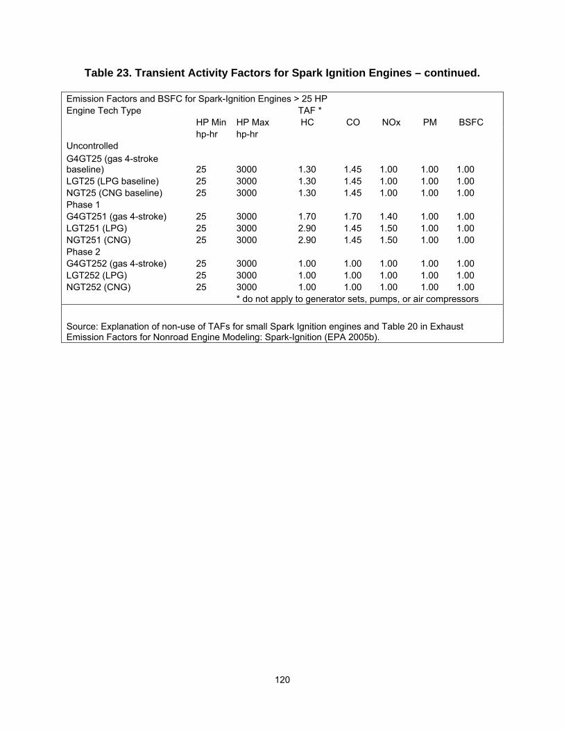
120
Table 23. Transient Activity Factors for Spark Ignition Engines – continued. Emission Factors and BSFC for Spark-Ignition Engines > 25 HP Engine Tech Type TAF *
HP Min HP Max HC CO NOx PM BSFC hp-hr hp-hr
Uncontrolled G4GT25 (gas 4-stroke baseline) 25 3000 1.30 1.45 1.00 1.00 1.00 LGT25 (LPG baseline) 25 3000 1.30 1.45 1.00 1.00 1.00 NGT25 (CNG baseline) 25 3000 1.30 1.45 1.00 1.00 1.00 Phase 1 G4GT251 (gas 4-stroke) 25 3000 1.70 1.70 1.40 1.00 1.00 LGT251 (LPG) 25 3000 2.90 1.45 1.50 1.00 1.00 NGT251 (CNG) 25 3000 2.90 1.45 1.50 1.00 1.00 Phase 2 G4GT252 (gas 4-stroke) 25 3000 1.00 1.00 1.00 1.00 1.00 LGT252 (LPG) 25 3000 1.00 1.00 1.00 1.00 1.00 NGT252 (CNG) 25 3000 1.00 1.00 1.00 1.00 1.00
* do not apply to generator sets, pumps, or air compressors
Source: Explanation of non-use of TAFs for small Spark Ignition engines and Table 20 in Exhaust Emission Factors for Nonroad Engine Modeling: Spark-Ignition (EPA 2005b).

121
Table 26. Deterioration Factors for Spark Ignition Engines.
Emissions and BSFC for Class III Handheld Small Spark Ignition Engines (< 20cc) Engine Tech Type Deterioration Factors A b
HP Min
HP Max HC CO NOx PM
BSFC
hp-hr hp-hr G2H3 (gas 2-stroke handheld Class III baseline) 0 1 0.2 0.2 0.000 0.000 0.000 1.000 G2H31 (Phase 1) 0 1 0.24 0.24 0.000 0.000 0.000 1.000 G2H3C1 (Phase 1 with catalyst) 0 1 0.24 0.24 0.000 0.000 0.000 1.000 G2H32 (Phase 2) 0 1 0.24 0.24 0.000 0.000 0.000 1.000 G2H3C2 (Phase 2 with catalysts) 0 1 0.24 0.24 0.000 0.000 0.000 1.000
Emissions and BSFC for Class IV Handheld Small Spark Ignition Engines (≥20cc and <50cc) Engine Tech Type Deterioration Factors A b
HP Min
HP Max HC CO NOx PM
BSFC
hp-hr hp-hr G2H4 (gas 2-stroke handheld Class IV baseline) 1 3 0.2 0.2 0.000 0.000 0.000 1.000 G2H41 (Phase 1) 1 3 0.29 0.24 0.000 0.000 0.000 1.000 G2H4C1 (Phase 1 with catalyst) 1 3 0.29 0.24 0.000 0.000 0.000 1.000 G4H41 (Phase 1 4-stroke) 1 3 1.1 0.9 -0.600 1.100 0.000 1.000 G2H42 (Phase 2) 1 3 0.29 0.24 0.000 0.000 0.000 1.000 G2H4C2 (Phase 2 with catalysts) 1 3 0.29 0.24 0.000 0.000 0.000 1.000 G4H42 (Phase 2 4-stroke) 1 3 1.1 0.9 -0.600 1.100 0.000 0.500
Emissions and BSFCs for Class V Handheld Small Spark Ignition Engines (>50cc) Engine Tech Type Deterioration Factors A b
HP Min
HP Max HC CO NOx PM
BSFC
hp-hr hp-hr G2H5 (gas 2-stroke handheld Class V baseline) 3 6 0.2 0.2 -0.031 0.000 0.000 1.000 G2H51 (Phase 1) 3 6 0.266 0.231 0.000 0.000 0.000 1.000 G2H5C1 (Phase 1 with catalyst) 3 6 0.266 0.231 0.000 0.000 0.000 1.000 G2H52 (Phase 2) 3 6 0.266 0.231 0.000 0.000 0.000 1.000 G2H5C2 (Phase 2 with catalysts) 3 6 0.266 0.231 0.000 0.000 0.000 1.000
Source: Tables 1-5,7 - Nonroad Spark-Ignition Engine Emission Deterioration Factors (EPA 2005f).
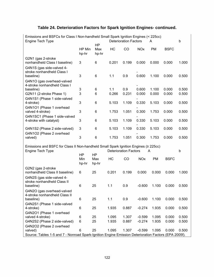
122
Table 24. Deterioration Factors for Spark Ignition Engines- continued.
Emissions and BSFCs for Class I Non-handheld Small Spark Ignition Engines (< 225cc) Engine Tech Type Deterioration Factors A b
HP Min HP Max HC CO NOx PM BSFC
hp-hr hp-hr G2N1 (gas 2-stroke nonhandheld Class I baseline) 3 6 0.201 0.199 0.000 0.000 0.000 1.000 G4N1S (gas side-valved 4-stroke nonhandheld Class I baseline) 3 6 1.1 0.9
-0.600 1.100 0.000 0.500
G4N1O (gas overhead-valved 4-stroke nonhandheld Class I baseline) 3 6 1.1 0.9
-0.600 1.100 0.000 0.500
G2N11 (2-stroke Phase 1) 3 6 0.266 0.231 0.000 0.000 0.000 0.500 G4N1S1 (Phase 1 side-valved 4-stroke) 3 6 5.103 1.109
-0.330 5.103 0.000 0.500
G4N1O1 (Phase 1 overhead valved 4-stroke) 3 6 1.753 1.051
-0.300 1.753 0.000 0.500
G4N1SC1 (Phase 1 side-valved 4-stroke with catalyst) 3 6 5.103 1.109
-0.330 5.103 0.000 0.500
G4N1S2 (Phase 2 side-valved) 3 6 5.103 1.109 -0.330 5.103 0.000 0.500
G4N1O2 (Phase 2 overhead valved) 3 6 1.753 1.051
-0.300 1.753 0.000 0.500
Emissions and BSFC for Class II Non-handheld Small Spark Ignition Engines (≥ 225cc) Engine Tech Type Deterioration Factors A b
HP Min
HP Max HC CO NOx PM
BSFC
hp-hr hp-hr G2N2 (gas 2-stroke nonhandheld Class II baseline) 6 25 0.201 0.199 0.000 0.000 0.000 1.000 G4N2S (gas side-valved 4-stroke nonhandheld Class II baseline) 6 25 1.1 0.9 -0.600 1.100 0.000 0.500 G4N2O (gas overhead-valved 4-stroke nonhandheld Class II baseline) 6 25 1.1 0.9 -0.600 1.100 0.000 0.500 G4N2S1 (Phase 1 side-valved 4-stroke) 6 25 1.935 0.887 -0.274 1.935 0.000 0.500 G4N2O1 (Phase 1 overhead valved 4-stroke) 6 25 1.095 1.307 -0.599 1.095 0.000 0.500 G4N2S2 (Phase 2 side-valved) 6 25 1.935 0.887 -0.274 1.935 0.000 0.500 G4N2O2 (Phase 2 overhead valved) 6 25 1.095 1.307 -0.599 1.095 0.000 0.500 Source: Tables 1-5 and 7 - Nonroad Spark-Ignition Engine Emission Deterioration Factors (EPA 2005f).

123
Table 24. Deterioration Factors for Spark Ignition Engines- continued.
Emission Factors and BSFC for Spark-Ignition Engines > 25 HP Engine Tech Type Deterioration Factors A b
HP Min HP Max HC CO NOx PM
BSFC
hp-hr hp-hr Uncontrolled
G4GT25 (gas 4-stroke baseline) 25 3000 1.1 0.9 -0.600 1.100 0.000 0.500 LGT25 (LPG baseline) 25 3000 1.1 0.9 -0.600 1.100 0.000 0.500 NGT25 (CNG baseline) 25 3000 1.1 0.9 -0.600 1.100 0.000 0.500 Phase 1 G4GT251 (gas 4-stroke) 25 3000 1.1 0.9 -0.600 1.100 0.000 0.500 LGT251 (LPG) 25 3000 1.1 0.9 -0.600 1.100 0.000 0.500 NGT251 (CNG) 25 3000 1.1 0.9 -0.600 1.100 0.000 0.500 Phase 2 G4GT252 (gas 4-stroke) 25 3000 1.1 0.9 -0.600 1.100 0.000 0.500 LGT252 (LPG) 25 3000 1.1 0.9 -0.600 1.100 0.000 0.500 NGT252 (CNG) 25 3000 1.1 0.9 -0.600 1.100 0.000 0.500
Source: Tables 1-5 and 7 - Nonroad Spark-Ignition Engine Emission Deterioration Factors (EPA 2005f).

124
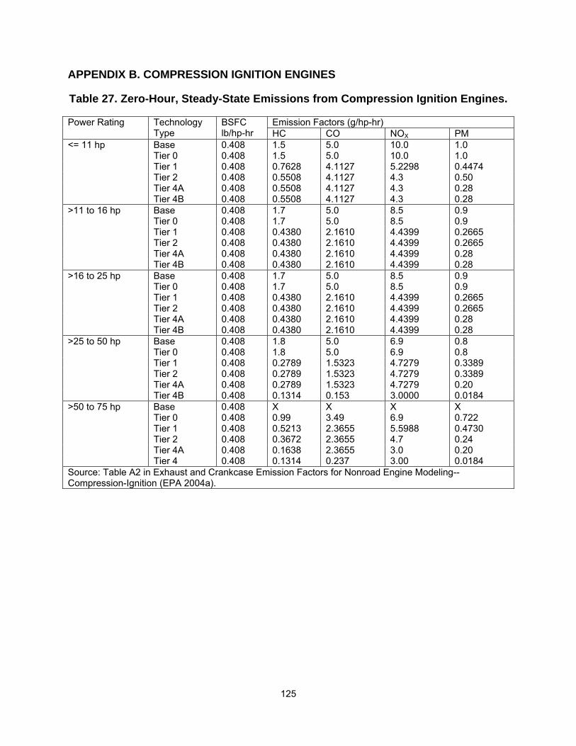
125
APPENDIX B. COMPRESSION IGNITION ENGINES
Table 27. Zero-Hour, Steady-State Emissions from Compression Ignition Engines.
Power Rating Technology Type
BSFC lb/hp-hr
Emission Factors (g/hp-hr) HC CO NOX PM
<= 11 hp Base 0.408 1.5 5.0 10.0 1.0 Tier 0 0.408 1.5 5.0 10.0 1.0 Tier 1 0.408 0.7628 4.1127 5.2298 0.4474 Tier 2 0.408 0.5508 4.1127 4.3 0.50 Tier 4A 0.408 0.5508 4.1127 4.3 0.28 Tier 4B 0.408 0.5508 4.1127 4.3 0.28 >11 to 16 hp Base 0.408 1.7 5.0 8.5 0.9 Tier 0 0.408 1.7 5.0 8.5 0.9 Tier 1 0.408 0.4380 2.1610 4.4399 0.2665 Tier 2 0.408 0.4380 2.1610 4.4399 0.2665 Tier 4A 0.408 0.4380 2.1610 4.4399 0.28 Tier 4B 0.408 0.4380 2.1610 4.4399 0.28 >16 to 25 hp Base 0.408 1.7 5.0 8.5 0.9 Tier 0 0.408 1.7 5.0 8.5 0.9 Tier 1 0.408 0.4380 2.1610 4.4399 0.2665 Tier 2 0.408 0.4380 2.1610 4.4399 0.2665 Tier 4A 0.408 0.4380 2.1610 4.4399 0.28 Tier 4B 0.408 0.4380 2.1610 4.4399 0.28 >25 to 50 hp Base 0.408 1.8 5.0 6.9 0.8 Tier 0 0.408 1.8 5.0 6.9 0.8 Tier 1 0.408 0.2789 1.5323 4.7279 0.3389 Tier 2 0.408 0.2789 1.5323 4.7279 0.3389 Tier 4A 0.408 0.2789 1.5323 4.7279 0.20 Tier 4B 0.408 0.1314 0.153 3.0000 0.0184 >50 to 75 hp Base 0.408 X X X X Tier 0 0.408 0.99 3.49 6.9 0.722 Tier 1 0.408 0.5213 2.3655 5.5988 0.4730 Tier 2 0.408 0.3672 2.3655 4.7 0.24 Tier 4A 0.408 0.1638 2.3655 3.0 0.20 Tier 4 0.408 0.1314 0.237 3.00 0.0184 Source: Table A2 in Exhaust and Crankcase Emission Factors for Nonroad Engine Modeling--Compression-Ignition (EPA 2004a).

126
Table 25. Zero-Hour, Steady-State Emissions from Compression Ignition Engines – continued.
Power Rating Technology Type
BSFC lb/hp-hr
Emission Factors (g/hp-hr) HC CO NOX PM
>75 to 100 hp Base 0.408 X X X X Tier 0 0.408 0.99 3.49 6.9 0.722 Tier 1 0.408 0.5213 2.3655 5.5988 0.4730 Tier 2 0.408 0.3672 2.3655 4.7 0.24 Tier 3B 0.408 0.1836 2.3655 3.0000 0.30 Tier 4 0.408 0.1314 0.237 3.00 0.0092 Tier 4N 0.408 0.1314 0.237 0.276 0.0092 >100 to 175 hp Base 0.367 X X X X Tier 0 0.367 0.68 2.70 8.38 0.402 Tier 1 0.367 0.3384 0.8667 5.6523 0.2799 Tier 2 0.367 0.3384 0.8667 4.1 0.18 Tier 3 0.367 0.1836 0.8667 2.5 0.22 Tier 4 0.367 0.1314 0.087 2.5 0.0092 Tier 4N 0.367 0.1314 0.087 0.276 0.0092 >175 to 300 hp Base 0.367 X X X X Tier 0 0.367 0.68 2.70 8.38 0.402 Tier 1 0.367 0.3085 0.7475 5.5772 0.2521 Tier 2 0.367 0.3085 0.7475 4.0 0.1316 Tier 3 0.367 0.1836 0.7475 2.5 0.15 Tier 4 0.367 0.1314 0.075 2.50 0.0092 Tier 4N 0.367 0.1314 0.075 0.276 0.0092 >300 to 600 hp Base 0.367 X X X X Tier 0 0.367 0.68 2.70 8.38 0.402 Tier 1 0.367 0.2025 1.3060 6.0153 0.2008 Tier 2 0.367 0.1669 0.8425 4.3351 0.1316 Tier 3 0.367 0.1669 0.8425 2.5 0.15 Tier 4 0.367 0.1314 0.084 2.50 0.0092 Tier 4N 0.367 0.1314 0.084 0.276 0.0092 Source: Table A2 in Exhaust and Crankcase Emission Factors for Nonroad Engine Modeling--Compression-Ignition (EPA 2004a)(EPA 2004a)(EPA 2004a).

127
Table 25. Zero-Hour, Steady-State Emissions from Compression Ignition Engines – continued.
Power Rating Technology Type
BSFC lb/hp-hr
Emission Factors (g/hp-hr) HC CO NOX PM
>600 to 750 Base 0.367 X X X X Tier 0 0.367 0.68 2.70 8.38 0.402 Tier 1 0.367 0.1473 1.3272 5.8215 0.2201 Tier 2 0.367 0.1669 1.3272 4.1 0.1316 Tier 3 0.367 0.1669 1.3272 2.5 0.15 Tier 4 0.367 0.1314 0.133 2.50 0.0092 Tier 4N 0.367 0.1314 0.133 0.276 0.0092 >750 hp Base 0.367 X X X X (except generators)
Tier 0 0.367 0.68 2.70 8.38 0.402
Tier 1 0.367 0.2861 0.7642 6.1525 0.1934 Tier 2 0.367 0.1669 1.3272 4.1 0.1316 Tier 4 0.367 0.2815 0.076 2.392 0.069 Tier 4N 0.367 0.1314 0.076 2.392 0.0276 Generator Sets Base 0.367 X X X X >750 to 1200 hp Tier 0 0.367 0.68 2.70 8.38 0.402 Tier 1 0.367 0.2861 0.7642 6.1525 0.1934 Tier 2 0.367 0.1669 0.7642 4.1 0.1316 Tier 4 0.367 0.2815 0.076 2.392 0.069 Tier 4N 0.367 0.1314 0.076 0.460 0.0184 Generator Sets Base 0.367 X X X X >1200 hp Tier 0 0.367 0.68 2.70 8.38 0.402 Tier 1 0.367 0.2861 0.7642 6.1525 0.1934 Tier 2 0.367 0.1669 0.7642 4.1 0.1316 Tier 4 0.367 0.2815 0.076 0.460 0.069 Tier 4N 0.367 0.1314 0.076 0.460 0.0184 Source: Table A2 in Exhaust and Crankcase Emission Factors for Nonroad Engine Modeling--Compression-Ignition (EPA 2004a).
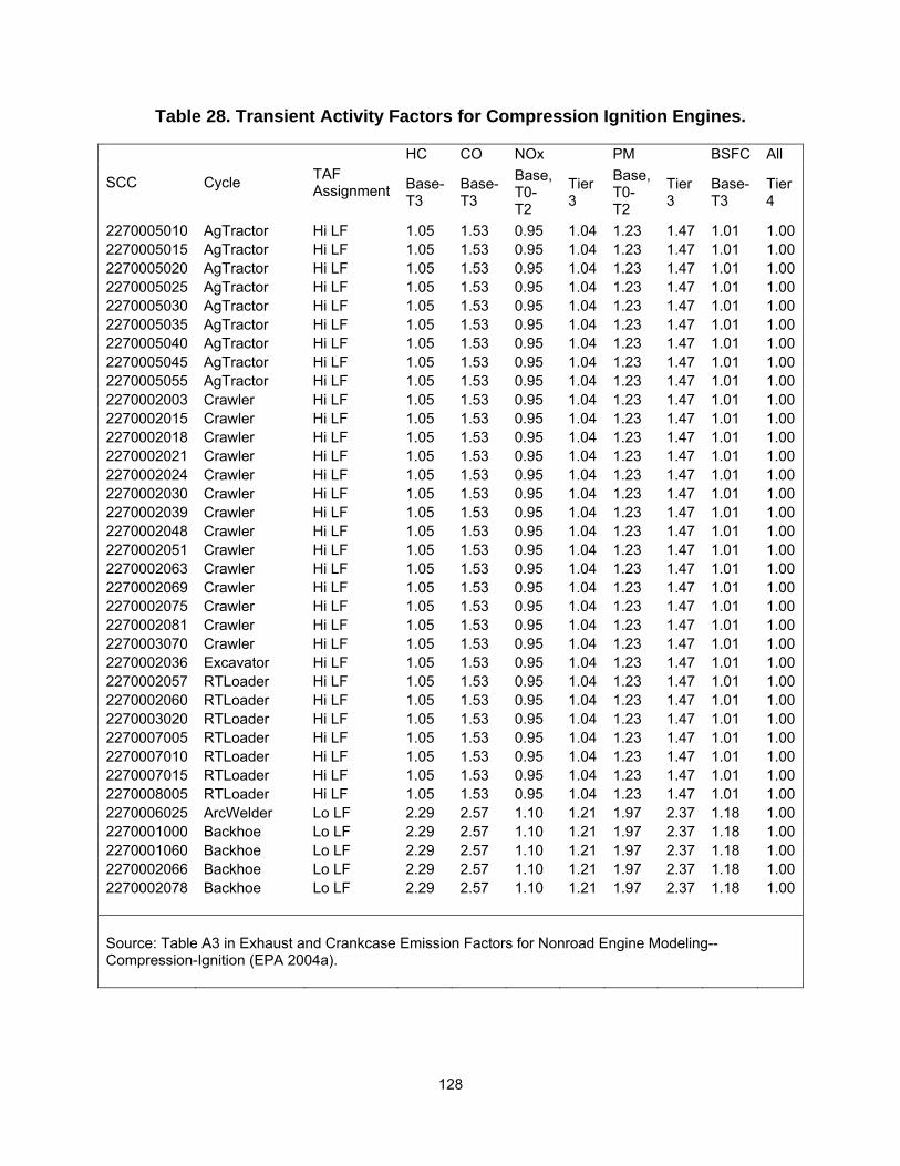
128
Table 28. Transient Activity Factors for Compression Ignition Engines.
SCC Cycle TAF Assignment
HC CO NOx PM BSFC All
Base-T3
Base-T3
Base, T0-T2
Tier 3
Base, T0-T2
Tier 3
Base-T3
Tier 4
2270005010 AgTractor Hi LF 1.05 1.53 0.95 1.04 1.23 1.47 1.01 1.002270005015 AgTractor Hi LF 1.05 1.53 0.95 1.04 1.23 1.47 1.01 1.002270005020 AgTractor Hi LF 1.05 1.53 0.95 1.04 1.23 1.47 1.01 1.002270005025 AgTractor Hi LF 1.05 1.53 0.95 1.04 1.23 1.47 1.01 1.002270005030 AgTractor Hi LF 1.05 1.53 0.95 1.04 1.23 1.47 1.01 1.002270005035 AgTractor Hi LF 1.05 1.53 0.95 1.04 1.23 1.47 1.01 1.002270005040 AgTractor Hi LF 1.05 1.53 0.95 1.04 1.23 1.47 1.01 1.002270005045 AgTractor Hi LF 1.05 1.53 0.95 1.04 1.23 1.47 1.01 1.002270005055 AgTractor Hi LF 1.05 1.53 0.95 1.04 1.23 1.47 1.01 1.002270002003 Crawler Hi LF 1.05 1.53 0.95 1.04 1.23 1.47 1.01 1.002270002015 Crawler Hi LF 1.05 1.53 0.95 1.04 1.23 1.47 1.01 1.002270002018 Crawler Hi LF 1.05 1.53 0.95 1.04 1.23 1.47 1.01 1.002270002021 Crawler Hi LF 1.05 1.53 0.95 1.04 1.23 1.47 1.01 1.002270002024 Crawler Hi LF 1.05 1.53 0.95 1.04 1.23 1.47 1.01 1.002270002030 Crawler Hi LF 1.05 1.53 0.95 1.04 1.23 1.47 1.01 1.002270002039 Crawler Hi LF 1.05 1.53 0.95 1.04 1.23 1.47 1.01 1.002270002048 Crawler Hi LF 1.05 1.53 0.95 1.04 1.23 1.47 1.01 1.002270002051 Crawler Hi LF 1.05 1.53 0.95 1.04 1.23 1.47 1.01 1.002270002063 Crawler Hi LF 1.05 1.53 0.95 1.04 1.23 1.47 1.01 1.002270002069 Crawler Hi LF 1.05 1.53 0.95 1.04 1.23 1.47 1.01 1.002270002075 Crawler Hi LF 1.05 1.53 0.95 1.04 1.23 1.47 1.01 1.002270002081 Crawler Hi LF 1.05 1.53 0.95 1.04 1.23 1.47 1.01 1.002270003070 Crawler Hi LF 1.05 1.53 0.95 1.04 1.23 1.47 1.01 1.002270002036 Excavator Hi LF 1.05 1.53 0.95 1.04 1.23 1.47 1.01 1.002270002057 RTLoader Hi LF 1.05 1.53 0.95 1.04 1.23 1.47 1.01 1.002270002060 RTLoader Hi LF 1.05 1.53 0.95 1.04 1.23 1.47 1.01 1.002270003020 RTLoader Hi LF 1.05 1.53 0.95 1.04 1.23 1.47 1.01 1.002270007005 RTLoader Hi LF 1.05 1.53 0.95 1.04 1.23 1.47 1.01 1.002270007010 RTLoader Hi LF 1.05 1.53 0.95 1.04 1.23 1.47 1.01 1.002270007015 RTLoader Hi LF 1.05 1.53 0.95 1.04 1.23 1.47 1.01 1.002270008005 RTLoader Hi LF 1.05 1.53 0.95 1.04 1.23 1.47 1.01 1.002270006025 ArcWelder Lo LF 2.29 2.57 1.10 1.21 1.97 2.37 1.18 1.002270001000 Backhoe Lo LF 2.29 2.57 1.10 1.21 1.97 2.37 1.18 1.002270001060 Backhoe Lo LF 2.29 2.57 1.10 1.21 1.97 2.37 1.18 1.002270002066 Backhoe Lo LF 2.29 2.57 1.10 1.21 1.97 2.37 1.18 1.002270002078 Backhoe Lo LF 2.29 2.57 1.10 1.21 1.97 2.37 1.18 1.00 Source: Table A3 in Exhaust and Crankcase Emission Factors for Nonroad Engine Modeling--Compression-Ignition (EPA 2004a).

129
Table 26. Transient Activity Factors for Compression Ignition Engines – continued.
SCC Cycle TAF Assignment
HC CO NOx PM BSFC All
Base-T3
Base-T3
Base, T0-T2
Tier 3
Base, T0-T2
Tier 3
Base-T3
Tier 4
2270003010 Backhoe Lo LF 2.29 2.57 1.10 1.21 1.97 2.37 1.18 1.002270003050 Backhoe Lo LF 2.29 2.57 1.10 1.21 1.97 2.37 1.18 1.002270009010 Backhoe Lo LF 2.29 2.57 1.10 1.21 1.97 2.37 1.18 1.002285002015 Backhoe Lo LF 2.29 2.57 1.10 1.21 1.97 2.37 1.18 1.002270002072 SSLoader Lo LF 2.29 2.57 1.10 1.21 1.97 2.37 1.18 1.002270001020 None None 1.00 1.00 1.00 1.00 1.00 1.00 1.00 1.002270001030 None None 1.00 1.00 1.00 1.00 1.00 1.00 1.00 1.002270001040 None None 1.00 1.00 1.00 1.00 1.00 1.00 1.00 1.002270001050 None None 1.00 1.00 1.00 1.00 1.00 1.00 1.00 1.002270002006 None None 1.00 1.00 1.00 1.00 1.00 1.00 1.00 1.002270002009 None None 1.00 1.00 1.00 1.00 1.00 1.00 1.00 1.002270002027 None None 1.00 1.00 1.00 1.00 1.00 1.00 1.00 1.002270002033 None None 1.00 1.00 1.00 1.00 1.00 1.00 1.00 1.002270002042 None None 1.00 1.00 1.00 1.00 1.00 1.00 1.00 1.002270002045 None None 1.00 1.00 1.00 1.00 1.00 1.00 1.00 1.002270002054 None None 1.00 1.00 1.00 1.00 1.00 1.00 1.00 1.002270003030 None None 1.00 1.00 1.00 1.00 1.00 1.00 1.00 1.002270003040 None None 1.00 1.00 1.00 1.00 1.00 1.00 1.00 1.002270003060 None None 1.00 1.00 1.00 1.00 1.00 1.00 1.00 1.002270004000 None None 1.00 1.00 1.00 1.00 1.00 1.00 1.00 1.002270004010 None None 1.00 1.00 1.00 1.00 1.00 1.00 1.00 1.002270004011 None None 1.00 1.00 1.00 1.00 1.00 1.00 1.00 1.002270004015 None None 1.00 1.00 1.00 1.00 1.00 1.00 1.00 1.002270004016 None None 1.00 1.00 1.00 1.00 1.00 1.00 1.00 1.002270004020 None None 1.00 1.00 1.00 1.00 1.00 1.00 1.00 1.002270004021 None None 1.00 1.00 1.00 1.00 1.00 1.00 1.00 1.002270004025 None None 1.00 1.00 1.00 1.00 1.00 1.00 1.00 1.002270004026 None None 1.00 1.00 1.00 1.00 1.00 1.00 1.00 1.002270004030 None None 1.00 1.00 1.00 1.00 1.00 1.00 1.00 1.002270004031 None None 1.00 1.00 1.00 1.00 1.00 1.00 1.00 1.002270004035 None None 1.00 1.00 1.00 1.00 1.00 1.00 1.00 1.002270004036 None None 1.00 1.00 1.00 1.00 1.00 1.00 1.00 1.002270004040 None None 1.00 1.00 1.00 1.00 1.00 1.00 1.00 1.002270004041 None None 1.00 1.00 1.00 1.00 1.00 1.00 1.00 1.002270004045 None None 1.00 1.00 1.00 1.00 1.00 1.00 1.00 1.002270004046 None None 1.00 1.00 1.00 1.00 1.00 1.00 1.00 1.002270004050 None None 1.00 1.00 1.00 1.00 1.00 1.00 1.00 1.002270004051 None None 1.00 1.00 1.00 1.00 1.00 1.00 1.00 1.00 Source: Table A3 in Exhaust and Crankcase Emission Factors for Nonroad Engine Modeling--Compression-Ignition (EPA 2004a)
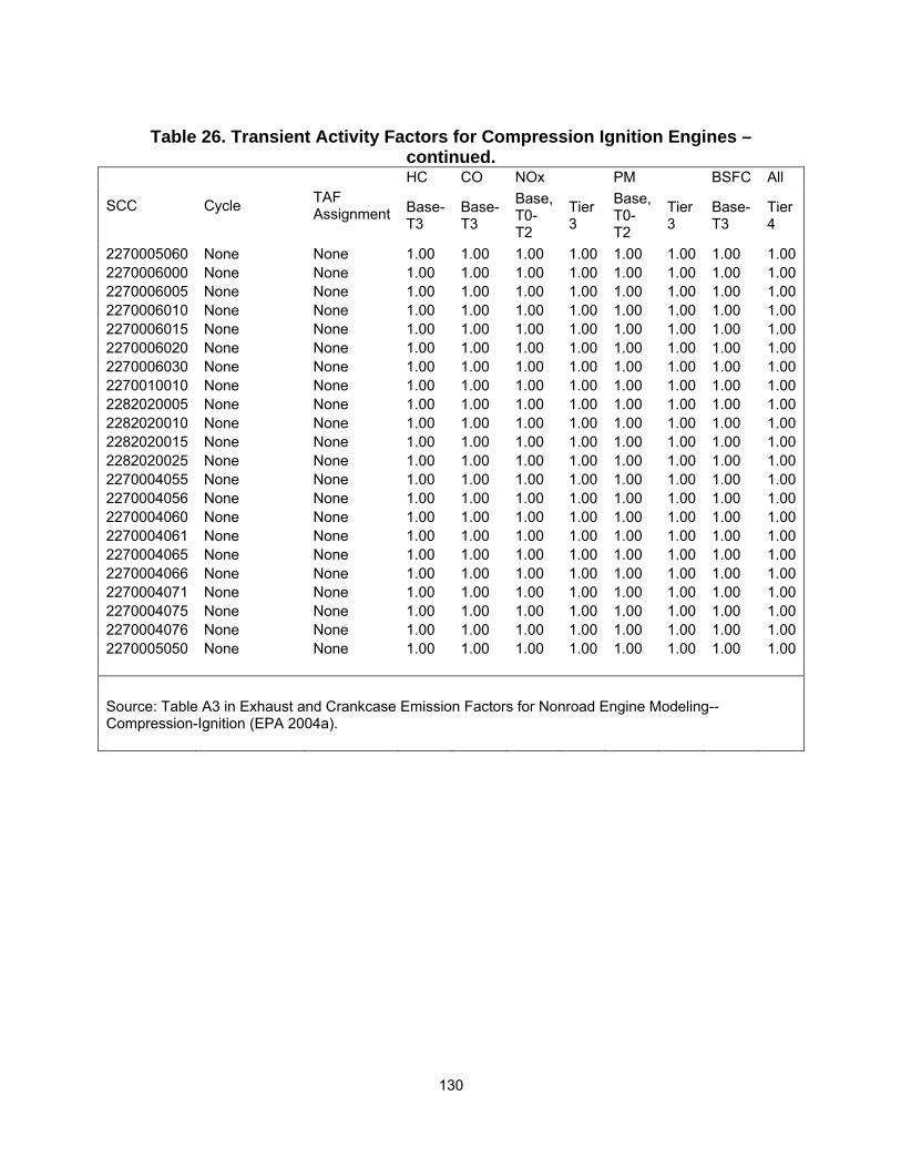
130
Table 26. Transient Activity Factors for Compression Ignition Engines –
continued.
SCC Cycle TAF Assignment
HC CO NOx PM BSFC All
Base-T3
Base-T3
Base, T0-T2
Tier 3
Base, T0-T2
Tier 3
Base-T3
Tier 4
2270005060 None None 1.00 1.00 1.00 1.00 1.00 1.00 1.00 1.002270006000 None None 1.00 1.00 1.00 1.00 1.00 1.00 1.00 1.002270006005 None None 1.00 1.00 1.00 1.00 1.00 1.00 1.00 1.002270006010 None None 1.00 1.00 1.00 1.00 1.00 1.00 1.00 1.002270006015 None None 1.00 1.00 1.00 1.00 1.00 1.00 1.00 1.002270006020 None None 1.00 1.00 1.00 1.00 1.00 1.00 1.00 1.002270006030 None None 1.00 1.00 1.00 1.00 1.00 1.00 1.00 1.002270010010 None None 1.00 1.00 1.00 1.00 1.00 1.00 1.00 1.002282020005 None None 1.00 1.00 1.00 1.00 1.00 1.00 1.00 1.002282020010 None None 1.00 1.00 1.00 1.00 1.00 1.00 1.00 1.002282020015 None None 1.00 1.00 1.00 1.00 1.00 1.00 1.00 1.002282020025 None None 1.00 1.00 1.00 1.00 1.00 1.00 1.00 1.002270004055 None None 1.00 1.00 1.00 1.00 1.00 1.00 1.00 1.002270004056 None None 1.00 1.00 1.00 1.00 1.00 1.00 1.00 1.002270004060 None None 1.00 1.00 1.00 1.00 1.00 1.00 1.00 1.002270004061 None None 1.00 1.00 1.00 1.00 1.00 1.00 1.00 1.002270004065 None None 1.00 1.00 1.00 1.00 1.00 1.00 1.00 1.002270004066 None None 1.00 1.00 1.00 1.00 1.00 1.00 1.00 1.002270004071 None None 1.00 1.00 1.00 1.00 1.00 1.00 1.00 1.002270004075 None None 1.00 1.00 1.00 1.00 1.00 1.00 1.00 1.002270004076 None None 1.00 1.00 1.00 1.00 1.00 1.00 1.00 1.002270005050 None None 1.00 1.00 1.00 1.00 1.00 1.00 1.00 1.00 Source: Table A3 in Exhaust and Crankcase Emission Factors for Nonroad Engine Modeling--Compression-Ignition (EPA 2004a).

131
Table 29. Compression Ignition Deterioration Factors.
Pollutant Relative Deterioration Factor (A) (% increase/%useful life)
b Base/ Tier 0
Tier 1 Tier 2 Tier 3 or later
HC 0.047 0.036 0.034 0.027 1.0 CO 0.185 0.101 0.101 0.151 1.0 NOX 0.024 0.024 0.009 0.008 1.0 PM 0.473 0.473 0.473 0.473 1.0 Source: Table A4 in Exhaust and Crankcase Emission Factors for Nonroad Engine Modeling--Compression-Ignition (EPA 2004a).

132
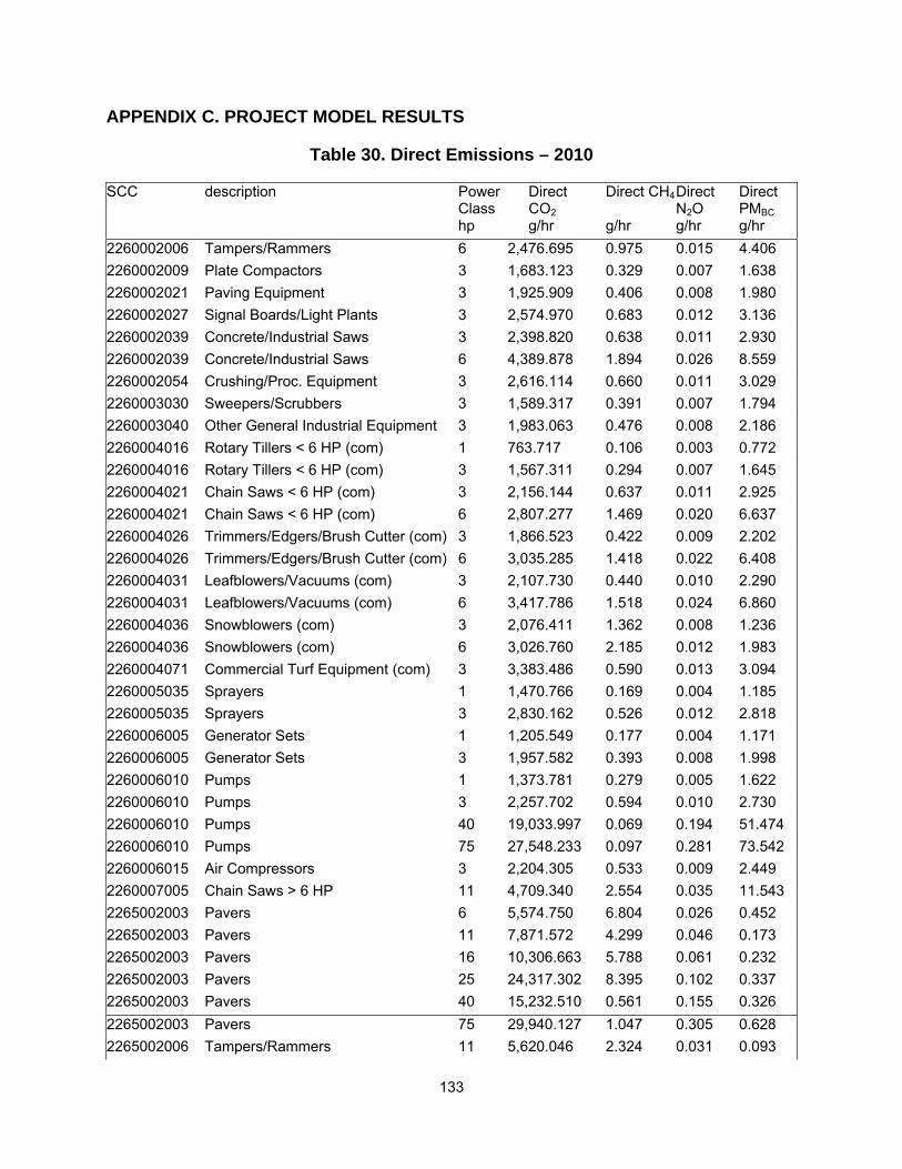
133
APPENDIX C. PROJECT MODEL RESULTS
Table 30. Direct Emissions – 2010
SCC description Power Class
Direct CO2
Direct CH4 Direct N2O
Direct PMBC
hp g/hr g/hr g/hr g/hr 2260002006 Tampers/Rammers 6 2,476.695 0.975 0.015 4.406 2260002009 Plate Compactors 3 1,683.123 0.329 0.007 1.638 2260002021 Paving Equipment 3 1,925.909 0.406 0.008 1.980 2260002027 Signal Boards/Light Plants 3 2,574.970 0.683 0.012 3.136 2260002039 Concrete/Industrial Saws 3 2,398.820 0.638 0.011 2.930 2260002039 Concrete/Industrial Saws 6 4,389.878 1.894 0.026 8.559 2260002054 Crushing/Proc. Equipment 3 2,616.114 0.660 0.011 3.029 2260003030 Sweepers/Scrubbers 3 1,589.317 0.391 0.007 1.794 2260003040 Other General Industrial Equipment 3 1,983.063 0.476 0.008 2.186 2260004016 Rotary Tillers < 6 HP (com) 1 763.717 0.106 0.003 0.772 2260004016 Rotary Tillers < 6 HP (com) 3 1,567.311 0.294 0.007 1.645 2260004021 Chain Saws < 6 HP (com) 3 2,156.144 0.637 0.011 2.925 2260004021 Chain Saws < 6 HP (com) 6 2,807.277 1.469 0.020 6.637 2260004026 Trimmers/Edgers/Brush Cutter (com) 3 1,866.523 0.422 0.009 2.202 2260004026 Trimmers/Edgers/Brush Cutter (com) 6 3,035.285 1.418 0.022 6.408 2260004031 Leafblowers/Vacuums (com) 3 2,107.730 0.440 0.010 2.290 2260004031 Leafblowers/Vacuums (com) 6 3,417.786 1.518 0.024 6.860 2260004036 Snowblowers (com) 3 2,076.411 1.362 0.008 1.236 2260004036 Snowblowers (com) 6 3,026.760 2.185 0.012 1.983 2260004071 Commercial Turf Equipment (com) 3 3,383.486 0.590 0.013 3.094 2260005035 Sprayers 1 1,470.766 0.169 0.004 1.185 2260005035 Sprayers 3 2,830.162 0.526 0.012 2.818 2260006005 Generator Sets 1 1,205.549 0.177 0.004 1.171 2260006005 Generator Sets 3 1,957.582 0.393 0.008 1.998 2260006010 Pumps 1 1,373.781 0.279 0.005 1.622 2260006010 Pumps 3 2,257.702 0.594 0.010 2.730 2260006010 Pumps 40 19,033.997 0.069 0.194 51.474 2260006010 Pumps 75 27,548.233 0.097 0.281 73.542 2260006015 Air Compressors 3 2,204.305 0.533 0.009 2.449 2260007005 Chain Saws > 6 HP 11 4,709.340 2.554 0.035 11.543 2265002003 Pavers 6 5,574.750 6.804 0.026 0.452 2265002003 Pavers 11 7,871.572 4.299 0.046 0.173 2265002003 Pavers 16 10,306.663 5.788 0.061 0.232 2265002003 Pavers 25 24,317.302 8.395 0.102 0.337 2265002003 Pavers 40 15,232.510 0.561 0.155 0.326 2265002003 Pavers 75 29,940.127 1.047 0.305 0.628 2265002006 Tampers/Rammers 11 5,620.046 2.324 0.031 0.093
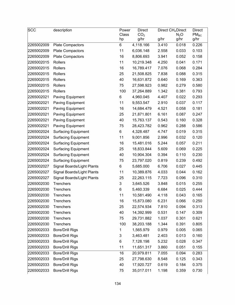
134
SCC description Power Class
Direct CO2
Direct CH4 Direct N2O
Direct PMBC
hp g/hr g/hr g/hr g/hr 2265002009 Plate Compactors 6 4,118.166 3.410 0.018 0.226 2265002009 Plate Compactors 11 6,036.148 2.558 0.033 0.103 2265002009 Plate Compactors 16 8,806.693 3.941 0.052 0.158 2265002015 Rollers 11 10,219.348 4.250 0.041 0.171 2265002015 Rollers 16 16,789.417 7.076 0.068 0.284 2265002015 Rollers 25 21,508.825 7.838 0.088 0.315 2265002015 Rollers 40 16,631.872 0.640 0.169 0.363 2265002015 Rollers 75 27,598.923 0.982 0.279 0.580 2265002015 Rollers 100 37,264.889 1.342 0.381 0.793 2265002021 Paving Equipment 6 4,960.045 4.407 0.022 0.293 2265002021 Paving Equipment 11 9,553.547 2.910 0.037 0.117 2265002021 Paving Equipment 16 14,684.479 4.521 0.058 0.181 2265002021 Paving Equipment 25 21,871.801 6.161 0.087 0.247 2265002021 Paving Equipment 40 15,763.137 0.543 0.160 0.328 2265002021 Paving Equipment 75 28,423.782 0.962 0.288 0.586 2265002024 Surfacing Equipment 6 4,328.487 4.747 0.019 0.315 2265002024 Surfacing Equipment 11 9,001.856 2.996 0.032 0.120 2265002024 Surfacing Equipment 16 15,481.016 5.244 0.057 0.211 2265002024 Surfacing Equipment 25 18,833.844 5.609 0.069 0.225 2265002024 Surfacing Equipment 40 10,904.304 0.394 0.110 0.230 2265002024 Surfacing Equipment 75 23,797.020 0.819 0.239 0.492 2265002027 Signal Boards/Light Plants 6 5,685.000 6.706 0.027 0.445 2265002027 Signal Boards/Light Plants 11 10,389.876 4.033 0.044 0.162 2265002027 Signal Boards/Light Plants 25 22,263.115 7.723 0.096 0.310 2265002030 Trenchers 3 3,645.526 3.848 0.015 0.255 2265002030 Trenchers 6 5,460.339 6.684 0.025 0.444 2265002030 Trenchers 11 10,581.490 4.118 0.043 0.165 2265002030 Trenchers 16 15,873.080 6.231 0.066 0.250 2265002030 Trenchers 25 22,574.934 7.810 0.094 0.313 2265002030 Trenchers 40 14,392.999 0.531 0.147 0.309 2265002030 Trenchers 75 29,731.882 1.037 0.301 0.621 2265002030 Trenchers 100 38,203.188 1.344 0.391 0.805 2265002033 Bore/Drill Rigs 1 1,565.979 0.979 0.005 0.065 2265002033 Bore/Drill Rigs 3 3,463.481 2.403 0.013 0.160 2265002033 Bore/Drill Rigs 6 7,128.198 5.232 0.028 0.347 2265002033 Bore/Drill Rigs 11 11,651.317 3.860 0.051 0.155 2265002033 Bore/Drill Rigs 16 20,979.811 7.055 0.094 0.283 2265002033 Bore/Drill Rigs 25 27,798.630 8.548 0.125 0.343 2265002033 Bore/Drill Rigs 40 17,920.727 0.619 0.184 0.375 2265002033 Bore/Drill Rigs 75 35,017.011 1.198 0.359 0.730
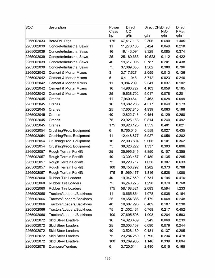
135
SCC description Power Class
Direct CO2
Direct CH4 Direct N2O
Direct PMBC
hp g/hr g/hr g/hr g/hr 2265002033 Bore/Drill Rigs 175 67,417.118 2.306 0.690 1.405 2265002039 Concrete/Industrial Saws 11 11,278.183 5.424 0.049 0.218 2265002039 Concrete/Industrial Saws 16 19,143.094 9.328 0.085 0.374 2265002039 Concrete/Industrial Saws 25 25,180.685 10.523 0.112 0.422 2265002039 Concrete/Industrial Saws 40 19,617.005 0.787 0.201 0.438 2265002039 Concrete/Industrial Saws 75 37,089.858 1.362 0.380 0.796 2265002042 Cement & Mortar Mixers 3 3,717.627 2.055 0.013 0.136 2265002042 Cement & Mortar Mixers 6 6,411.048 3.712 0.023 0.246 2265002042 Cement & Mortar Mixers 11 9,384.209 2.541 0.037 0.102 2265002042 Cement & Mortar Mixers 16 14,960.727 4.103 0.059 0.165 2265002042 Cement & Mortar Mixers 25 19,638.702 5.017 0.078 0.201 2265002045 Cranes 11 7,960.464 2.463 0.028 0.099 2265002045 Cranes 16 13,682.285 4.317 0.049 0.173 2265002045 Cranes 25 17,607.810 4.939 0.063 0.198 2265002045 Cranes 40 12,822.746 0.454 0.129 0.268 2265002045 Cranes 75 23,925.158 0.814 0.240 0.492 2265002045 Cranes 175 39,920.125 1.359 0.401 0.821 2265002054 Crushing/Proc. Equipment 6 6,765.045 6.558 0.027 0.435 2265002054 Crushing/Proc. Equipment 11 12,448.877 5.027 0.056 0.202 2265002054 Crushing/Proc. Equipment 16 22,003.804 9.006 0.101 0.362 2265002054 Crushing/Proc. Equipment 75 38,326.222 1.337 0.393 0.806 2265002057 Rough Terrain Forklift 25 25,995.645 8.850 0.107 0.355 2265002057 Rough Terrain Forklift 40 13,303.457 0.489 0.135 0.285 2265002057 Rough Terrain Forklift 75 30,229.717 1.056 0.307 0.633 2265002057 Rough Terrain Forklift 100 36,456.792 1.282 0.373 0.768 2265002057 Rough Terrain Forklift 175 51,969.177 1.816 0.528 1.088 2265002060 Rubber Tire Loaders 40 19,047.559 0.731 0.194 0.416 2265002060 Rubber Tire Loaders 75 36,240.278 1.298 0.370 0.768 2265002060 Rubber Tire Loaders 175 58,168.321 2.083 0.594 1.233 2265002066 Tractors/Loaders/Backhoes 11 10,665.864 4.078 0.038 0.164 2265002066 Tractors/Loaders/Backhoes 25 18,654.385 6.179 0.068 0.248 2265002066 Tractors/Loaders/Backhoes 40 10,607.298 0.409 0.107 0.230 2265002066 Tractors/Loaders/Backhoes 75 21,302.431 0.768 0.217 0.452 2265002066 Tractors/Loaders/Backhoes 100 27,695.598 1.008 0.284 0.593 2265002072 Skid Steer Loaders 16 14,320.439 5.949 0.068 0.239 2265002072 Skid Steer Loaders 25 20,003.157 6.090 0.079 0.244 2265002072 Skid Steer Loaders 40 13,528.180 0.481 0.137 0.285 2265002072 Skid Steer Loaders 75 23,284.250 0.790 0.234 0.478 2265002072 Skid Steer Loaders 100 33,269.935 1.146 0.339 0.694 2265002078 Dumpers/Tenders 6 3,720.514 2.480 0.015 0.165

136
SCC description Power Class
Direct CO2
Direct CH4 Direct N2O
Direct PMBC
hp g/hr g/hr g/hr g/hr 2265002078 Dumpers/Tenders 11 7,899.443 1.809 0.026 0.073 2265002078 Dumpers/Tenders 16 11,292.725 2.608 0.037 0.105 2265002078 Dumpers/Tenders 25 16,944.762 3.676 0.057 0.148 2265002078 Dumpers/Tenders 75 20,095.754 0.669 0.200 0.407 2265002081 Other Construction Equipment 25 17,653.175 4.920 0.064 0.197 2265002081 Other Construction Equipment 175 44,545.739 1.513 0.448 0.915 2265003010 Aerial Lifts 11 6,926.658 2.352 0.027 0.094 2265003010 Aerial Lifts 16 10,190.520 4.192 0.049 0.168 2265003010 Aerial Lifts 25 20,118.519 5.468 0.072 0.219 2265003010 Aerial Lifts 40 10,601.118 0.371 0.106 0.220 2265003010 Aerial Lifts 75 20,324.563 0.687 0.204 0.416 2265003010 Aerial Lifts 175 37,856.426 1.280 0.380 0.775 2265003020 Forklifts 40 8,265.899 0.281 0.080 0.167 2265003020 Forklifts 50 10,167.073 0.352 0.100 0.208 2265003020 Forklifts 75 13,870.582 0.489 0.139 0.289 2265003020 Forklifts 100 19,393.155 0.693 0.198 0.410 2265003020 Forklifts 175 31,100.912 1.126 0.321 0.667 2265003020 Forklifts 300 46,053.615 1.680 0.479 0.995 2265003030 Sweepers/Scrubbers 6 6,551.514 7.298 0.025 0.484 2265003030 Sweepers/Scrubbers 11 12,209.846 5.320 0.052 0.214 2265003030 Sweepers/Scrubbers 16 18,256.193 8.017 0.078 0.322 2265003030 Sweepers/Scrubbers 25 22,343.067 8.484 0.096 0.341 2265003030 Sweepers/Scrubbers 40 16,427.602 0.631 0.168 0.359 2265003030 Sweepers/Scrubbers 50 23,680.182 0.910 0.242 0.518 2265003030 Sweepers/Scrubbers 75 32,615.819 1.169 0.333 0.692 2265003030 Sweepers/Scrubbers 100 45,879.816 1.660 0.473 0.983 2265003030 Sweepers/Scrubbers 175 77,213.809 2.767 0.788 1.638 2265003030 Sweepers/Scrubbers 600 211,562.230 7.582 2.159 4.487 2265003040 Other General Industrial Eqp 6 5,064.937 5.117 0.017 0.340 2265003040 Other General Industrial Eqp 11 9,626.296 3.769 0.036 0.151 2265003040 Other General Industrial Eqp 16 14,242.359 5.627 0.054 0.226 2265003040 Other General Industrial Eqp 25 19,041.547 6.526 0.073 0.262 2265003040 Other General Industrial Eqp 40 11,916.646 0.456 0.120 0.259 2265003040 Other General Industrial Eqp 75 24,156.633 0.858 0.244 0.507 2265003040 Other General Industrial Eqp 100 31,364.103 1.127 0.320 0.665 2265003040 Other General Industrial Eqp 175 53,800.543 1.915 0.543 1.131 2265003040 Other General Industrial Eqp 300 77,139.637 2.746 0.779 1.622 2265003050 Other Material Handling Eqp 3 3,622.242 2.838 0.012 0.188 2265003050 Other Material Handling Eqp 25 18,732.690 5.605 0.071 0.225 2265003050 Other Material Handling Eqp 75 24,781.006 0.840 0.247 0.506

137
SCC description Power Class
Direct CO2
Direct CH4 Direct N2O
Direct PMBC
hp g/hr g/hr g/hr g/hr 2265003050 Other Material Handling Eqp 100 33,326.261 1.146 0.337 0.691 2265003060 AC\Refrigeration 11 8,821.249 2.941 0.031 0.118 2265003060 AC\Refrigeration 16 12,630.842 4.248 0.044 0.171 2265003060 AC\Refrigeration 25 17,296.790 5.125 0.061 0.206 2265004011 Lawn mowers (Com) 3 1,681.251 1.213 0.006 0.081 2265004011 Lawn mowers (Com) 6 2,327.699 1.950 0.010 0.129 2265004011 Lawn mowers (Com) 11 2,919.008 1.249 0.015 0.050 2265004016 Rotary Tillers < 6 HP (com) 6 2,909.536 2.227 0.014 0.148 2265004026 Trimmers/Edgers/Brush Cutter (com) 6 4,166.065 4.167 0.022 0.277 2265004026 Trimmers/Edgers/Brush Cutter (com) 11 8,567.677 4.596 0.053 0.184 2265004026 Trimmers/Edgers/Brush Cutter (com) 16 17,082.958 9.309 0.108 0.374 2265004026 Trimmers/Edgers/Brush Cutter (com) 25 19,144.454 10.473 0.121 0.420 2265004031 Leafblowers/Vacuums (com) 6 4,919.403 4.435 0.024 0.294 2265004031 Leafblowers/Vacuums (com) 11 9,401.982 4.988 0.058 0.200 2265004031 Leafblowers/Vacuums (com) 16 15,532.254 8.534 0.099 0.343 2265004031 Leafblowers/Vacuums (com) 25 22,525.502 12.621 0.146 0.507 2265004031 Leafblowers/Vacuums (com) 40 20,627.222 0.782 0.216 0.454 2265004031 Leafblowers/Vacuums (com) 75 40,704.986 1.465 0.426 0.877 2265004031 Leafblowers/Vacuums (com) 175 80,308.390 2.891 0.840 1.731 2265004036 Snowblowers (com) 11 5,158.948 4.092 0.023 0.069 2265004036 Snowblowers (com) 16 7,180.315 5.923 0.033 0.100 2265004041 Rear Engine Riding Mowers (com) 6 3,687.006 3.525 0.014 0.234 2265004041 Rear Engine Riding Mowers (com) 11 6,280.569 2.122 0.026 0.085 2265004041 Rear Engine Riding Mowers (com) 16 7,841.605 2.923 0.035 0.117 2265004041 Rear Engine Riding Mowers (com) 25 10,627.757 4.091 0.051 0.164 2265004046 Front Mowers (com) 11 7,310.456 2.721 0.038 0.109 2265004046 Front Mowers (com) 16 12,091.699 4.582 0.065 0.184 2265004046 Front Mowers (com) 25 15,037.054 5.329 0.082 0.214 2265004046 Front Mowers (com) 40 14,904.323 0.518 0.155 0.316 2265004051 Shredders < 6 HP (com) 3 3,559.210 2.743 0.018 0.182 2265004051 Shredders < 6 HP (com) 6 5,439.278 4.442 0.029 0.295 2265004056 Lawn & Garden Tractors (com) 6 5,169.756 4.544 0.016 0.302 2265004056 Lawn & Garden Tractors (com) 11 7,185.166 2.613 0.032 0.105 2265004056 Lawn & Garden Tractors (com) 16 9,165.269 3.653 0.044 0.147 2265004056 Lawn & Garden Tractors (com) 25 11,870.220 4.941 0.060 0.198 2265004066 Chippers/Stump Grinders (com) 6 5,242.828 6.007 0.020 0.399 2265004066 Chippers/Stump Grinders (com) 11 12,445.996 5.864 0.057 0.235 2265004066 Chippers/Stump Grinders (com) 16 17,210.206 9.176 0.088 0.368 2265004066 Chippers/Stump Grinders (com) 25 26,369.888 10.336 0.116 0.415 2265004066 Chippers/Stump Grinders (com) 40 19,796.534 0.767 0.203 0.435

138
SCC description Power Class
Direct CO2
Direct CH4 Direct N2O
Direct PMBC
hp g/hr g/hr g/hr g/hr 2265004066 Chippers/Stump Grinders (com) 75 34,272.031 1.235 0.351 0.730 2265004066 Chippers/Stump Grinders (com) 100 44,787.789 1.626 0.462 0.961 2265004066 Chippers/Stump Grinders (com) 175 67,098.307 2.418 0.687 1.429 2265004071 Commercial Turf Equipment (com) 6 6,340.090 4.287 0.023 0.285 2265004071 Commercial Turf Equipment (com) 11 9,916.324 3.330 0.039 0.134 2265004071 Commercial Turf Equipment (com) 16 13,420.177 5.312 0.062 0.213 2265004071 Commercial Turf Equipment (com) 25 20,826.655 7.339 0.086 0.295 2265004071 Commercial Turf Equipment (com) 40 11,772.380 0.463 0.121 0.261 2265004071 Commercial Turf Equipment (com) 75 25,386.776 0.937 0.265 0.552 2265004076 Other Lawn & Garden Eqp. (com) 1 3,093.222 0.593 0.004 0.039 2265004076 Other Lawn & Garden Eqp. (com) 3 4,126.817 1.518 0.010 0.101 2265004076 Other Lawn & Garden Eqp. (com) 6 5,958.432 3.157 0.021 0.210 2265004076 Other Lawn & Garden Eqp. (com) 11 9,792.366 2.343 0.035 0.094 2265004076 Other Lawn & Garden Eqp. (com) 16 14,498.411 4.436 0.067 0.178 2265004076 Other Lawn & Garden Eqp. (com) 25 21,515.428 5.342 0.086 0.214 2265004076 Other Lawn & Garden Eqp. (com) 40 14,996.715 0.517 0.155 0.315 2265004076 Other Lawn & Garden Eqp. (com) 75 27,184.323 0.946 0.283 0.576 2265004076 Other Lawn & Garden Eqp. (com) 100 35,320.281 1.233 0.369 0.751 2265004076 Other Lawn & Garden Eqp. (com) 175 46,303.801 1.620 0.485 0.987 2265005010 2-Wheel Tractors 11 8,375.850 3.263 0.038 0.131 2265005010 2-Wheel Tractors 16 12,501.134 5.648 0.065 0.227 2265005015 Agricultural Tractors 25 22,931.064 8.163 0.094 0.328 2265005015 Agricultural Tractors 40 13,777.495 0.522 0.140 0.298 2265005015 Agricultural Tractors 100 36,439.477 1.316 0.377 0.781 2265005015 Agricultural Tractors 175 55,265.298 2.003 0.574 1.189 2265005030 Agricultural Mowers 6 6,021.493 3.960 0.021 0.263 2265005030 Agricultural Mowers 11 7,328.971 2.464 0.033 0.099 2265005030 Agricultural Mowers 16 10,970.228 4.282 0.057 0.172 2265005030 Agricultural Mowers 25 12,444.424 4.384 0.064 0.176 2265005035 Sprayers 6 5,149.606 3.463 0.021 0.230 2265005035 Sprayers 11 9,989.426 2.762 0.039 0.111 2265005035 Sprayers 16 14,762.777 4.999 0.071 0.201 2265005035 Sprayers 25 23,719.988 6.377 0.099 0.256 2265005035 Sprayers 40 15,733.346 0.535 0.160 0.326 2265005035 Sprayers 75 29,551.749 0.996 0.298 0.607 2265005035 Sprayers 100 42,250.848 1.444 0.432 0.880 2265005035 Sprayers 175 61,593.642 2.093 0.627 1.275 2265005040 Tillers > 6 HP 11 6,576.025 2.392 0.039 0.096 2265005040 Tillers > 6 HP 16 12,748.400 4.708 0.078 0.189 2265005045 Swathers 100 30,526.965 1.028 0.308 0.626

139
SCC description Power Class
Direct CO2
Direct CH4 Direct N2O
Direct PMBC
hp g/hr g/hr g/hr g/hr 2265005045 Swathers 175 46,514.413 1.567 0.469 0.955 2265005055 Other Agricultural Equipment 6 3,854.790 3.468 0.020 0.230 2265005055 Other Agricultural Equipment 11 9,662.033 2.710 0.037 0.109 2265005055 Other Agricultural Equipment 16 12,738.693 4.184 0.057 0.168 2265005055 Other Agricultural Equipment 25 19,642.859 5.063 0.076 0.203 2265005055 Other Agricultural Equipment 40 12,977.623 0.440 0.131 0.267 2265005055 Other Agricultural Equipment 75 25,175.663 0.848 0.254 0.517 2265005055 Other Agricultural Equipment 100 35,069.028 1.197 0.358 0.729 2265005055 Other Agricultural Equipment 175 66,213.846 2.275 0.681 1.386 2265005055 Other Agricultural Equipment 300 90,387.778 3.128 0.937 1.906 2265005060 Irrigation Sets 6 4,253.864 6.304 0.021 0.418 2265005060 Irrigation Sets 11 7,000.064 4.241 0.040 0.170 2265005060 Irrigation Sets 75 26,366.517 0.942 0.265 0.554 2265005060 Irrigation Sets 100 35,009.790 1.267 0.356 0.744 2265005060 Irrigation Sets 175 52,737.164 1.902 0.535 1.118 2265005060 Irrigation Sets 300 91,993.011 3.318 0.933 1.950 2265006005 Generator Sets 6 4,930.709 4.190 0.023 0.278 2265006005 Generator Sets 11 10,730.701 3.304 0.044 0.133 2265006005 Generator Sets 16 17,232.011 5.373 0.072 0.216 2265006005 Generator Sets 25 24,647.508 7.081 0.104 0.284 2265006010 Pumps 6 5,038.377 5.205 0.024 0.345 2265006010 Pumps 11 10,472.212 3.580 0.043 0.144 2265006010 Pumps 16 15,404.489 6.359 0.076 0.255 2265006010 Pumps 25 22,124.413 7.022 0.094 0.282 2265006010 Pumps 40 16,000.494 0.566 0.163 0.337 2265006010 Pumps 50 23,035.697 0.815 0.235 0.486 2265006010 Pumps 75 30,249.386 1.040 0.309 0.631 2265006010 Pumps 100 40,237.824 1.395 0.415 0.847 2265006010 Pumps 175 57,174.964 1.980 0.589 1.201 2265006015 Air Compressors 6 4,927.678 5.686 0.021 0.377 2265006015 Air Compressors 11 10,261.461 3.924 0.041 0.157 2265006015 Air Compressors 16 12,634.133 5.388 0.056 0.216 2265006015 Air Compressors 25 19,221.099 6.437 0.077 0.258 2265006015 Air Compressors 40 13,119.109 0.477 0.131 0.277 2265006015 Air Compressors 75 24,777.711 0.867 0.252 0.519 2265006015 Air Compressors 100 33,005.881 1.166 0.339 0.698 2265006015 Air Compressors 175 53,183.881 1.883 0.547 1.127 2265006025 Welders 6 6,707.062 8.014 0.030 0.532 2265006025 Welders 11 8,565.532 4.502 0.047 0.181 2265006025 Welders 16 13,374.118 7.584 0.079 0.304
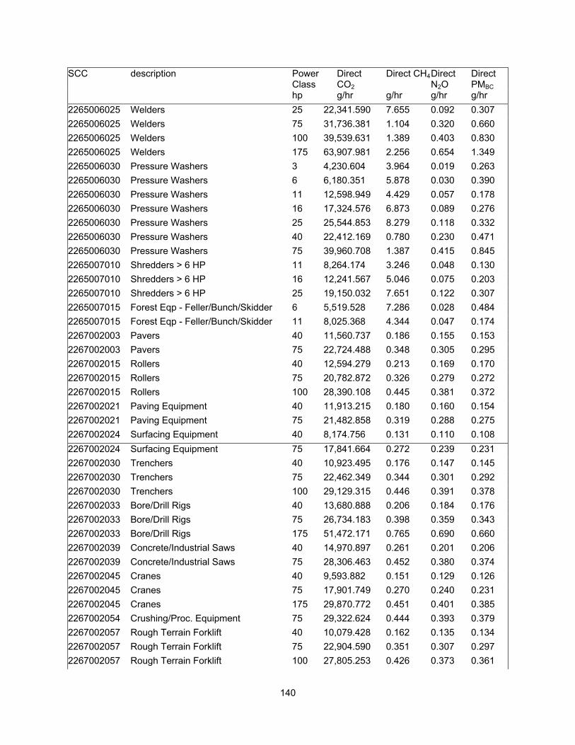
140
SCC description Power Class
Direct CO2
Direct CH4 Direct N2O
Direct PMBC
hp g/hr g/hr g/hr g/hr 2265006025 Welders 25 22,341.590 7.655 0.092 0.307 2265006025 Welders 75 31,736.381 1.104 0.320 0.660 2265006025 Welders 100 39,539.631 1.389 0.403 0.830 2265006025 Welders 175 63,907.981 2.256 0.654 1.349 2265006030 Pressure Washers 3 4,230.604 3.964 0.019 0.263 2265006030 Pressure Washers 6 6,180.351 5.878 0.030 0.390 2265006030 Pressure Washers 11 12,598.949 4.429 0.057 0.178 2265006030 Pressure Washers 16 17,324.576 6.873 0.089 0.276 2265006030 Pressure Washers 25 25,544.853 8.279 0.118 0.332 2265006030 Pressure Washers 40 22,412.169 0.780 0.230 0.471 2265006030 Pressure Washers 75 39,960.708 1.387 0.415 0.845 2265007010 Shredders > 6 HP 11 8,264.174 3.246 0.048 0.130 2265007010 Shredders > 6 HP 16 12,241.567 5.046 0.075 0.203 2265007010 Shredders > 6 HP 25 19,150.032 7.651 0.122 0.307 2265007015 Forest Eqp - Feller/Bunch/Skidder 6 5,519.528 7.286 0.028 0.484 2265007015 Forest Eqp - Feller/Bunch/Skidder 11 8,025.368 4.344 0.047 0.174 2267002003 Pavers 40 11,560.737 0.186 0.155 0.153 2267002003 Pavers 75 22,724.488 0.348 0.305 0.295 2267002015 Rollers 40 12,594.279 0.213 0.169 0.170 2267002015 Rollers 75 20,782.872 0.326 0.279 0.272 2267002015 Rollers 100 28,390.108 0.445 0.381 0.372 2267002021 Paving Equipment 40 11,913.215 0.180 0.160 0.154 2267002021 Paving Equipment 75 21,482.858 0.319 0.288 0.275 2267002024 Surfacing Equipment 40 8,174.756 0.131 0.110 0.108 2267002024 Surfacing Equipment 75 17,841.664 0.272 0.239 0.231 2267002030 Trenchers 40 10,923.495 0.176 0.147 0.145 2267002030 Trenchers 75 22,462.349 0.344 0.301 0.292 2267002030 Trenchers 100 29,129.315 0.446 0.391 0.378 2267002033 Bore/Drill Rigs 40 13,680.888 0.206 0.184 0.176 2267002033 Bore/Drill Rigs 75 26,734.183 0.398 0.359 0.343 2267002033 Bore/Drill Rigs 175 51,472.171 0.765 0.690 0.660 2267002039 Concrete/Industrial Saws 40 14,970.897 0.261 0.201 0.206 2267002039 Concrete/Industrial Saws 75 28,306.463 0.452 0.380 0.374 2267002045 Cranes 40 9,593.882 0.151 0.129 0.126 2267002045 Cranes 75 17,901.749 0.270 0.240 0.231 2267002045 Cranes 175 29,870.772 0.451 0.401 0.385 2267002054 Crushing/Proc. Equipment 75 29,322.624 0.444 0.393 0.379 2267002057 Rough Terrain Forklift 40 10,079.428 0.162 0.135 0.134 2267002057 Rough Terrain Forklift 75 22,904.590 0.351 0.307 0.297 2267002057 Rough Terrain Forklift 100 27,805.253 0.426 0.373 0.361
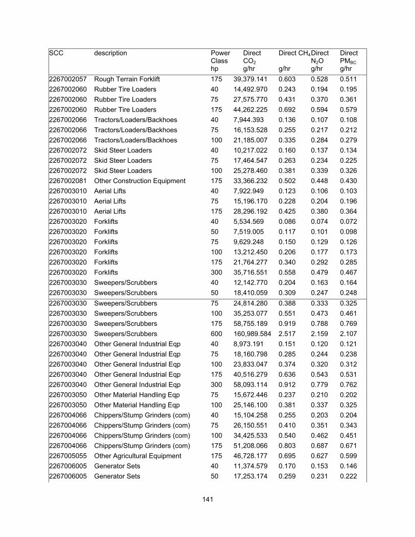
141
SCC description Power Class
Direct CO2
Direct CH4 Direct N2O
Direct PMBC
hp g/hr g/hr g/hr g/hr 2267002057 Rough Terrain Forklift 175 39,379.141 0.603 0.528 0.511 2267002060 Rubber Tire Loaders 40 14,492.970 0.243 0.194 0.195 2267002060 Rubber Tire Loaders 75 27,575.770 0.431 0.370 0.361 2267002060 Rubber Tire Loaders 175 44,262.225 0.692 0.594 0.579 2267002066 Tractors/Loaders/Backhoes 40 7,944.393 0.136 0.107 0.108 2267002066 Tractors/Loaders/Backhoes 75 16,153.528 0.255 0.217 0.212 2267002066 Tractors/Loaders/Backhoes 100 21,185.007 0.335 0.284 0.279 2267002072 Skid Steer Loaders 40 10,217.022 0.160 0.137 0.134 2267002072 Skid Steer Loaders 75 17,464.547 0.263 0.234 0.225 2267002072 Skid Steer Loaders 100 25,278.460 0.381 0.339 0.326 2267002081 Other Construction Equipment 175 33,366.232 0.502 0.448 0.430 2267003010 Aerial Lifts 40 7,922.949 0.123 0.106 0.103 2267003010 Aerial Lifts 75 15,196.170 0.228 0.204 0.196 2267003010 Aerial Lifts 175 28,296.192 0.425 0.380 0.364 2267003020 Forklifts 40 5,534.569 0.086 0.074 0.072 2267003020 Forklifts 50 7,519.005 0.117 0.101 0.098 2267003020 Forklifts 75 9,629.248 0.150 0.129 0.126 2267003020 Forklifts 100 13,212.450 0.206 0.177 0.173 2267003020 Forklifts 175 21,764.277 0.340 0.292 0.285 2267003020 Forklifts 300 35,716.551 0.558 0.479 0.467 2267003030 Sweepers/Scrubbers 40 12,142.770 0.204 0.163 0.164 2267003030 Sweepers/Scrubbers 50 18,410.059 0.309 0.247 0.248 2267003030 Sweepers/Scrubbers 75 24,814.280 0.388 0.333 0.325 2267003030 Sweepers/Scrubbers 100 35,253.077 0.551 0.473 0.461 2267003030 Sweepers/Scrubbers 175 58,755.189 0.919 0.788 0.769 2267003030 Sweepers/Scrubbers 600 160,989.584 2.517 2.159 2.107 2267003040 Other General Industrial Eqp 40 8,973.191 0.151 0.120 0.121 2267003040 Other General Industrial Eqp 75 18,160.798 0.285 0.244 0.238 2267003040 Other General Industrial Eqp 100 23,833.047 0.374 0.320 0.312 2267003040 Other General Industrial Eqp 175 40,516.279 0.636 0.543 0.531 2267003040 Other General Industrial Eqp 300 58,093.114 0.912 0.779 0.762 2267003050 Other Material Handling Eqp 75 15,672.446 0.237 0.210 0.202 2267003050 Other Material Handling Eqp 100 25,146.100 0.381 0.337 0.325 2267004066 Chippers/Stump Grinders (com) 40 15,104.258 0.255 0.203 0.204 2267004066 Chippers/Stump Grinders (com) 75 26,150.551 0.410 0.351 0.343 2267004066 Chippers/Stump Grinders (com) 100 34,425.533 0.540 0.462 0.451 2267004066 Chippers/Stump Grinders (com) 175 51,208.066 0.803 0.687 0.671 2267005055 Other Agricultural Equipment 175 46,728.177 0.695 0.627 0.599 2267006005 Generator Sets 40 11,374.579 0.170 0.153 0.146 2267006005 Generator Sets 50 17,253.174 0.259 0.231 0.222

142
SCC description Power Class
Direct CO2
Direct CH4 Direct N2O
Direct PMBC
hp g/hr g/hr g/hr g/hr 2267006005 Generator Sets 75 23,600.689 0.351 0.317 0.303 2267006005 Generator Sets 100 30,492.106 0.453 0.409 0.391 2267006005 Generator Sets 175 52,070.729 0.774 0.698 0.668 2267006005 Generator Sets 300 89,885.788 1.337 1.206 1.152 2267006005 Generator Sets 600 139,555.746 2.075 1.872 1.789 2267006010 Pumps 40 12,162.268 0.188 0.163 0.158 2267006010 Pumps 50 17,510.664 0.270 0.235 0.228 2267006010 Pumps 75 21,697.989 0.325 0.291 0.279 2267006010 Pumps 100 30,929.124 0.463 0.415 0.398 2267006010 Pumps 175 43,890.875 0.657 0.589 0.564 2267006015 Air Compressors 40 9,784.336 0.158 0.131 0.130 2267006015 Air Compressors 75 18,762.376 0.288 0.252 0.244 2267006015 Air Compressors 100 25,237.902 0.387 0.339 0.328 2267006015 Air Compressors 175 40,750.079 0.625 0.547 0.529 2267006025 Welders 75 23,870.759 0.367 0.320 0.310 2267006025 Welders 100 30,011.965 0.461 0.403 0.390 2267006025 Welders 175 48,769.545 0.749 0.654 0.634 2267006030 Pressure Washers 40 17,139.610 0.259 0.230 0.221 2267006030 Pressure Washers 75 30,949.876 0.460 0.415 0.397 2268002081 Other Construction Equipment 175 24,197.638 78.271 0.373 0.358 2268003020 Forklifts 50 6,911.440 23.199 0.107 0.104 2268003030 Sweepers/Scrubbers 300 64,746.033 217.605 0.998 0.974 2268003040 Other General Industrial Eqp 100 25,528.040 86.117 0.394 0.385 2268003060 AC\Refrigeration 50 10,593.897 36.958 0.163 0.162 2268003060 AC\Refrigeration 75 16,340.157 53.953 0.252 0.244 2268006005 Generator Sets 40 10,359.435 33.359 0.160 0.153 2268006005 Generator Sets 50 15,563.704 50.117 0.240 0.230 2268006005 Generator Sets 75 19,734.157 63.065 0.304 0.291 2268006005 Generator Sets 100 31,152.154 99.553 0.480 0.459 2268006005 Generator Sets 175 48,258.000 154.218 0.744 0.711 2268006005 Generator Sets 300 78,296.727 250.214 1.207 1.153 2268006005 Generator Sets 600 128,186.972 409.649 1.976 1.888 2268006010 Pumps 40 10,598.505 35.184 0.163 0.159 2268006010 Pumps 75 17,227.171 55.428 0.266 0.254 2268006010 Pumps 175 57,976.066 186.537 0.894 0.856 2268006010 Pumps 300 81,497.699 262.218 1.256 1.204 2268006010 Pumps 600 140,235.749 451.206 2.161 2.071 2268006015 Air Compressors 75 13,978.646 46.087 0.215 0.209 2268006015 Air Compressors 175 39,785.294 131.170 0.613 0.594 2268006020 Gas Compressors 40 11,167.952 57.355 0.173 0.206

143
SCC description Power Class
Direct CO2
Direct CH4 Direct N2O
Direct PMBC
hp g/hr g/hr g/hr g/hr 2268006020 Gas Compressors 50 18,372.344 94.354 0.285 0.339 2268006020 Gas Compressors 75 28,021.479 143.908 0.434 0.517 2268006020 Gas Compressors 100 37,037.048 190.210 0.574 0.684 2268006020 Gas Compressors 175 59,251.196 304.294 0.918 1.094 2268006020 Gas Compressors 300 98,319.052 504.931 1.523 1.815 2268006020 Gas Compressors 600 163,214.693 838.215 2.528 3.013 2270002003 Pavers 25 7,703.616 0.091 0.096 1.571 2270002003 Pavers 40 11,537.282 0.087 0.143 1.704 2270002003 Pavers 50 15,948.208 0.120 0.198 2.356 2270002003 Pavers 75 22,145.314 0.107 0.275 3.138 2270002003 Pavers 100 30,478.772 0.159 0.378 9.676 2270002003 Pavers 175 42,633.746 0.247 0.588 9.512 2270002003 Pavers 300 70,032.116 0.406 0.965 9.916 2270002003 Pavers 600 122,546.923 0.634 1.689 17.009 2270002006 Tampers/Rammers 6 1,066.331 0.016 0.013 0.208 2270002009 Plate Compactors 6 1,253.453 0.019 0.016 0.245 2270002009 Plate Compactors 11 2,171.766 0.032 0.027 0.425 2270002009 Plate Compactors 16 3,610.187 0.043 0.045 0.707 2270002009 Plate Compactors 25 5,166.478 0.062 0.065 1.011 2270002015 Rollers 6 1,912.953 0.028 0.024 0.388 2270002015 Rollers 11 3,058.677 0.045 0.038 0.620 2270002015 Rollers 16 4,766.390 0.057 0.059 0.966 2270002015 Rollers 25 6,922.699 0.082 0.086 1.402 2270002015 Rollers 40 11,438.780 0.086 0.142 1.679 2270002015 Rollers 50 16,113.568 0.122 0.200 2.365 2270002015 Rollers 75 21,364.518 0.103 0.265 3.016 2270002015 Rollers 100 29,813.977 0.155 0.370 9.431 2270002015 Rollers 175 41,873.588 0.242 0.577 9.304 2270002015 Rollers 300 68,733.517 0.398 0.947 9.689 2270002015 Rollers 600 133,189.771 0.690 1.836 18.431 2270002018 Scrapers 75 23,214.619 0.112 0.288 3.307 2270002018 Scrapers 175 50,932.443 0.295 0.702 11.433 2270002018 Scrapers 300 78,204.117 0.453 1.078 11.148 2270002018 Scrapers 600 133,822.819 0.693 1.845 18.659 2270002018 Scrapers 750 217,791.519 1.128 3.002 30.367 2270002018 Scrapers 1000 240,723.011 1.247 3.318 21.935 2270002021 Paving Equipment 6 1,625.200 0.024 0.020 0.324 2270002021 Paving Equipment 11 2,567.951 0.038 0.032 0.513 2270002021 Paving Equipment 16 5,170.921 0.061 0.064 1.032 2270002021 Paving Equipment 25 6,936.771 0.082 0.086 1.385

144
SCC description Power Class
Direct CO2
Direct CH4 Direct N2O
Direct PMBC
hp g/hr g/hr g/hr g/hr 2270002021 Paving Equipment 40 11,896.075 0.090 0.148 1.720 2270002021 Paving Equipment 75 21,473.571 0.104 0.267 3.006 2270002021 Paving Equipment 100 29,275.776 0.153 0.363 9.186 2270002021 Paving Equipment 175 41,588.543 0.241 0.573 9.155 2270002021 Paving Equipment 300 72,914.513 0.422 1.005 10.176 2270002021 Paving Equipment 600 145,700.699 0.754 2.008 20.026 2270002024 Surfacing Equipment 11 2,356.888 0.035 0.029 0.467 2270002024 Surfacing Equipment 16 4,678.449 0.055 0.058 0.928 2270002024 Surfacing Equipment 25 7,619.197 0.090 0.095 1.511 2270002024 Surfacing Equipment 40 11,146.907 0.084 0.138 1.601 2270002024 Surfacing Equipment 50 15,793.428 0.119 0.196 2.268 2270002024 Surfacing Equipment 75 19,320.897 0.094 0.240 2.695 2270002024 Surfacing Equipment 100 28,456.228 0.148 0.353 8.897 2270002024 Surfacing Equipment 175 40,068.148 0.232 0.552 8.784 2270002024 Surfacing Equipment 300 73,801.438 0.427 1.017 10.254 2270002024 Surfacing Equipment 600 156,026.586 0.807 2.151 21.380 2270002024 Surfacing Equipment 750 225,994.842 1.169 3.115 30.967 2270002024 Surfacing Equipment 1000 284,117.011 1.471 3.916 25.392 2270002024 Surfacing Equipment 2000 489,048.706 2.531 6.741 43.706 2270002027 Signal Boards/Light Plants 6 1,371.004 0.020 0.017 0.270 2270002027 Signal Boards/Light Plants 11 1,973.989 0.029 0.025 0.388 2270002027 Signal Boards/Light Plants 16 3,485.783 0.042 0.044 0.685 2270002027 Signal Boards/Light Plants 25 5,631.083 0.067 0.071 1.107 2270002027 Signal Boards/Light Plants 40 7,697.314 0.059 0.096 1.096 2270002027 Signal Boards/Light Plants 50 10,713.278 0.081 0.134 1.525 2270002027 Signal Boards/Light Plants 75 15,048.937 0.074 0.189 2.099 2270002027 Signal Boards/Light Plants 100 22,594.121 0.113 0.283 4.745 2270002027 Signal Boards/Light Plants 175 35,966.348 0.199 0.501 5.003 2270002027 Signal Boards/Light Plants 300 49,325.303 0.273 0.687 4.086 2270002030 Trenchers 11 3,377.037 0.050 0.042 0.672 2270002030 Trenchers 16 5,452.329 0.065 0.068 1.085 2270002030 Trenchers 25 7,598.083 0.090 0.094 1.512 2270002030 Trenchers 40 11,994.566 0.090 0.149 1.728 2270002030 Trenchers 50 15,846.224 0.120 0.197 2.283 2270002030 Trenchers 75 21,462.944 0.104 0.266 3.000 2270002030 Trenchers 100 30,513.892 0.159 0.379 9.558 2270002030 Trenchers 175 42,538.789 0.246 0.586 9.346 2270002030 Trenchers 300 79,344.461 0.459 1.094 11.050 2270002030 Trenchers 600 131,320.700 0.680 1.810 18.023 2270002030 Trenchers 750 234,926.728 1.216 3.238 32.243
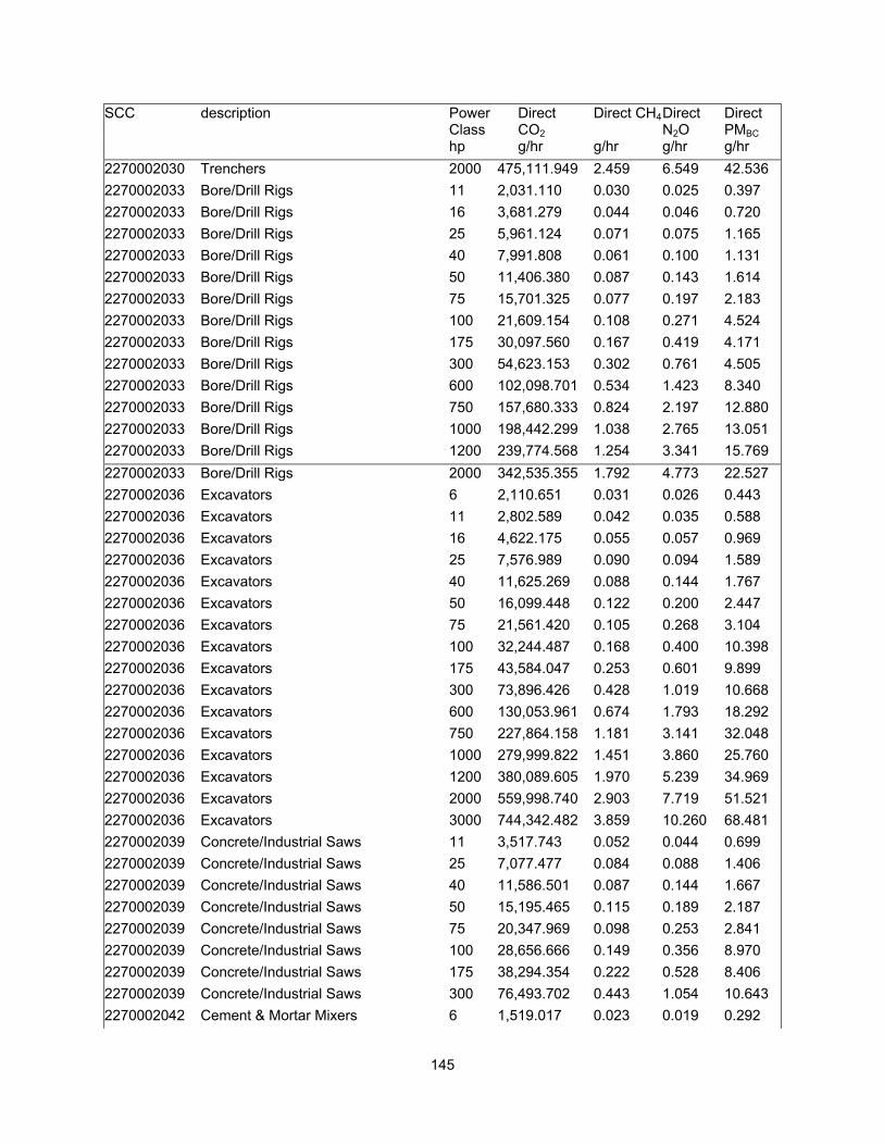
145
SCC description Power Class
Direct CO2
Direct CH4 Direct N2O
Direct PMBC
hp g/hr g/hr g/hr g/hr 2270002030 Trenchers 2000 475,111.949 2.459 6.549 42.536 2270002033 Bore/Drill Rigs 11 2,031.110 0.030 0.025 0.397 2270002033 Bore/Drill Rigs 16 3,681.279 0.044 0.046 0.720 2270002033 Bore/Drill Rigs 25 5,961.124 0.071 0.075 1.165 2270002033 Bore/Drill Rigs 40 7,991.808 0.061 0.100 1.131 2270002033 Bore/Drill Rigs 50 11,406.380 0.087 0.143 1.614 2270002033 Bore/Drill Rigs 75 15,701.325 0.077 0.197 2.183 2270002033 Bore/Drill Rigs 100 21,609.154 0.108 0.271 4.524 2270002033 Bore/Drill Rigs 175 30,097.560 0.167 0.419 4.171 2270002033 Bore/Drill Rigs 300 54,623.153 0.302 0.761 4.505 2270002033 Bore/Drill Rigs 600 102,098.701 0.534 1.423 8.340 2270002033 Bore/Drill Rigs 750 157,680.333 0.824 2.197 12.880 2270002033 Bore/Drill Rigs 1000 198,442.299 1.038 2.765 13.051 2270002033 Bore/Drill Rigs 1200 239,774.568 1.254 3.341 15.769 2270002033 Bore/Drill Rigs 2000 342,535.355 1.792 4.773 22.527 2270002036 Excavators 6 2,110.651 0.031 0.026 0.443 2270002036 Excavators 11 2,802.589 0.042 0.035 0.588 2270002036 Excavators 16 4,622.175 0.055 0.057 0.969 2270002036 Excavators 25 7,576.989 0.090 0.094 1.589 2270002036 Excavators 40 11,625.269 0.088 0.144 1.767 2270002036 Excavators 50 16,099.448 0.122 0.200 2.447 2270002036 Excavators 75 21,561.420 0.105 0.268 3.104 2270002036 Excavators 100 32,244.487 0.168 0.400 10.398 2270002036 Excavators 175 43,584.047 0.253 0.601 9.899 2270002036 Excavators 300 73,896.426 0.428 1.019 10.668 2270002036 Excavators 600 130,053.961 0.674 1.793 18.292 2270002036 Excavators 750 227,864.158 1.181 3.141 32.048 2270002036 Excavators 1000 279,999.822 1.451 3.860 25.760 2270002036 Excavators 1200 380,089.605 1.970 5.239 34.969 2270002036 Excavators 2000 559,998.740 2.903 7.719 51.521 2270002036 Excavators 3000 744,342.482 3.859 10.260 68.481 2270002039 Concrete/Industrial Saws 11 3,517.743 0.052 0.044 0.699 2270002039 Concrete/Industrial Saws 25 7,077.477 0.084 0.088 1.406 2270002039 Concrete/Industrial Saws 40 11,586.501 0.087 0.144 1.667 2270002039 Concrete/Industrial Saws 50 15,195.465 0.115 0.189 2.187 2270002039 Concrete/Industrial Saws 75 20,347.969 0.098 0.253 2.841 2270002039 Concrete/Industrial Saws 100 28,656.666 0.149 0.356 8.970 2270002039 Concrete/Industrial Saws 175 38,294.354 0.222 0.528 8.406 2270002039 Concrete/Industrial Saws 300 76,493.702 0.443 1.054 10.643 2270002042 Cement & Mortar Mixers 6 1,519.017 0.023 0.019 0.292
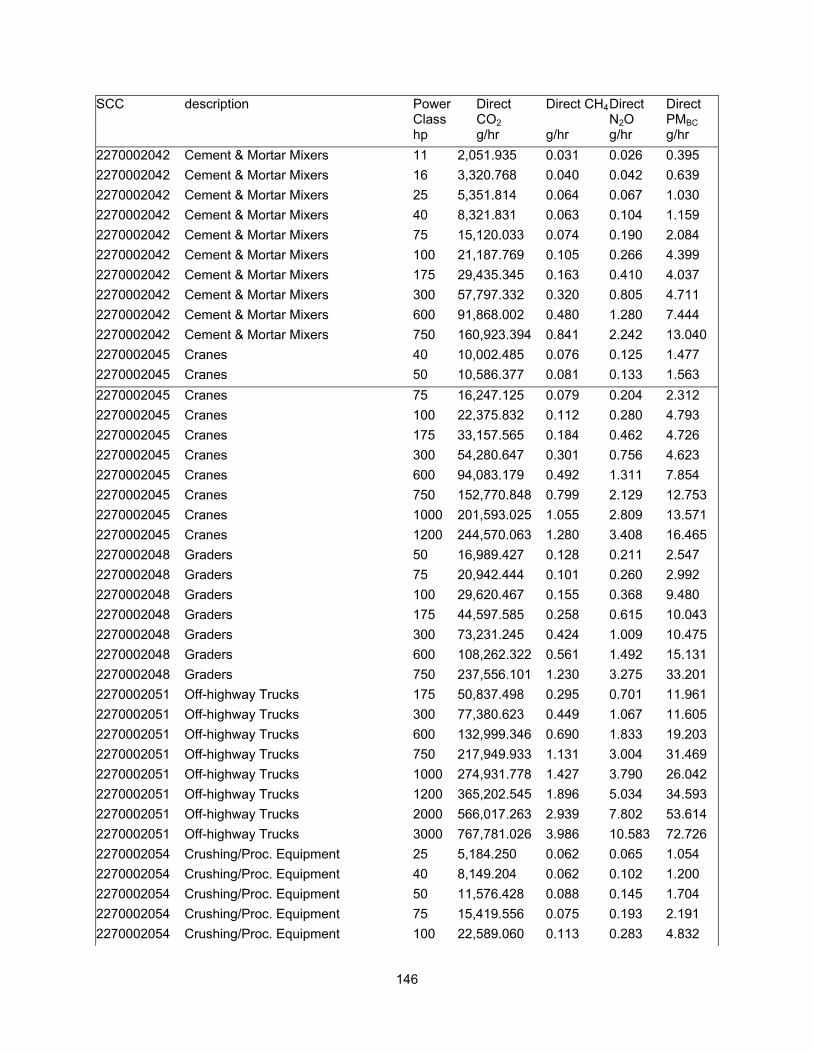
146
SCC description Power Class
Direct CO2
Direct CH4 Direct N2O
Direct PMBC
hp g/hr g/hr g/hr g/hr 2270002042 Cement & Mortar Mixers 11 2,051.935 0.031 0.026 0.395 2270002042 Cement & Mortar Mixers 16 3,320.768 0.040 0.042 0.639 2270002042 Cement & Mortar Mixers 25 5,351.814 0.064 0.067 1.030 2270002042 Cement & Mortar Mixers 40 8,321.831 0.063 0.104 1.159 2270002042 Cement & Mortar Mixers 75 15,120.033 0.074 0.190 2.084 2270002042 Cement & Mortar Mixers 100 21,187.769 0.105 0.266 4.399 2270002042 Cement & Mortar Mixers 175 29,435.345 0.163 0.410 4.037 2270002042 Cement & Mortar Mixers 300 57,797.332 0.320 0.805 4.711 2270002042 Cement & Mortar Mixers 600 91,868.002 0.480 1.280 7.444 2270002042 Cement & Mortar Mixers 750 160,923.394 0.841 2.242 13.040 2270002045 Cranes 40 10,002.485 0.076 0.125 1.477 2270002045 Cranes 50 10,586.377 0.081 0.133 1.563 2270002045 Cranes 75 16,247.125 0.079 0.204 2.312 2270002045 Cranes 100 22,375.832 0.112 0.280 4.793 2270002045 Cranes 175 33,157.565 0.184 0.462 4.726 2270002045 Cranes 300 54,280.647 0.301 0.756 4.623 2270002045 Cranes 600 94,083.179 0.492 1.311 7.854 2270002045 Cranes 750 152,770.848 0.799 2.129 12.753 2270002045 Cranes 1000 201,593.025 1.055 2.809 13.571 2270002045 Cranes 1200 244,570.063 1.280 3.408 16.465 2270002048 Graders 50 16,989.427 0.128 0.211 2.547 2270002048 Graders 75 20,942.444 0.101 0.260 2.992 2270002048 Graders 100 29,620.467 0.155 0.368 9.480 2270002048 Graders 175 44,597.585 0.258 0.615 10.043 2270002048 Graders 300 73,231.245 0.424 1.009 10.475 2270002048 Graders 600 108,262.322 0.561 1.492 15.131 2270002048 Graders 750 237,556.101 1.230 3.275 33.201 2270002051 Off-highway Trucks 175 50,837.498 0.295 0.701 11.961 2270002051 Off-highway Trucks 300 77,380.623 0.449 1.067 11.605 2270002051 Off-highway Trucks 600 132,999.346 0.690 1.833 19.203 2270002051 Off-highway Trucks 750 217,949.933 1.131 3.004 31.469 2270002051 Off-highway Trucks 1000 274,931.778 1.427 3.790 26.042 2270002051 Off-highway Trucks 1200 365,202.545 1.896 5.034 34.593 2270002051 Off-highway Trucks 2000 566,017.263 2.939 7.802 53.614 2270002051 Off-highway Trucks 3000 767,781.026 3.986 10.583 72.726 2270002054 Crushing/Proc. Equipment 25 5,184.250 0.062 0.065 1.054 2270002054 Crushing/Proc. Equipment 40 8,149.204 0.062 0.102 1.200 2270002054 Crushing/Proc. Equipment 50 11,576.428 0.088 0.145 1.704 2270002054 Crushing/Proc. Equipment 75 15,419.556 0.075 0.193 2.191 2270002054 Crushing/Proc. Equipment 100 22,589.060 0.113 0.283 4.832
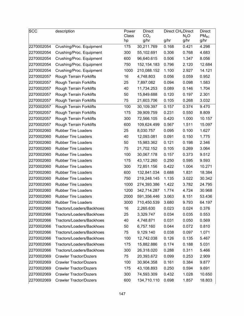
147
SCC description Power Class
Direct CO2
Direct CH4 Direct N2O
Direct PMBC
hp g/hr g/hr g/hr g/hr 2270002054 Crushing/Proc. Equipment 175 30,211.769 0.168 0.421 4.298 2270002054 Crushing/Proc. Equipment 300 55,102.691 0.306 0.768 4.683 2270002054 Crushing/Proc. Equipment 600 96,640.615 0.506 1.347 8.056 2270002054 Crushing/Proc. Equipment 750 152,154.183 0.796 2.120 12.684 2270002054 Crushing/Proc. Equipment 1000 210,088.152 1.100 2.927 14.121 2270002057 Rough Terrain Forklifts 16 4,748.803 0.056 0.059 0.952 2270002057 Rough Terrain Forklifts 25 7,897.082 0.094 0.098 1.583 2270002057 Rough Terrain Forklifts 40 11,734.253 0.089 0.146 1.704 2270002057 Rough Terrain Forklifts 50 15,849.688 0.120 0.197 2.301 2270002057 Rough Terrain Forklifts 75 21,603.706 0.105 0.268 3.032 2270002057 Rough Terrain Forklifts 100 30,109.397 0.157 0.374 9.470 2270002057 Rough Terrain Forklifts 175 39,909.759 0.231 0.550 8.809 2270002057 Rough Terrain Forklifts 300 72,566.105 0.420 1.000 10.157 2270002057 Rough Terrain Forklifts 600 109,624.499 0.567 1.511 15.097 2270002060 Rubber Tire Loaders 25 8,030.757 0.095 0.100 1.627 2270002060 Rubber Tire Loaders 40 12,093.081 0.091 0.150 1.775 2270002060 Rubber Tire Loaders 50 15,983.362 0.121 0.198 2.346 2270002060 Rubber Tire Loaders 75 21,702.152 0.105 0.269 3.064 2270002060 Rubber Tire Loaders 100 30,067.178 0.157 0.373 9.512 2270002060 Rubber Tire Loaders 175 43,172.260 0.250 0.595 9.593 2270002060 Rubber Tire Loaders 300 72,851.156 0.422 1.004 10.271 2270002060 Rubber Tire Loaders 600 132,841.034 0.688 1.831 18.384 2270002060 Rubber Tire Loaders 750 219,248.145 1.135 3.022 30.342 2270002060 Rubber Tire Loaders 1000 274,393.386 1.422 3.782 24.795 2270002060 Rubber Tire Loaders 1200 342,714.287 1.774 4.724 30.968 2270002060 Rubber Tire Loaders 2000 591,356.446 3.063 8.151 53.436 2270002060 Rubber Tire Loaders 3000 710,450.539 3.680 9.793 64.197 2270002066 Tractors/Loaders/Backhoes 16 2,265.630 0.023 0.024 0.376 2270002066 Tractors/Loaders/Backhoes 25 3,329.747 0.034 0.035 0.553 2270002066 Tractors/Loaders/Backhoes 40 4,748.871 0.031 0.050 0.569 2270002066 Tractors/Loaders/Backhoes 50 6,757.160 0.044 0.072 0.810 2270002066 Tractors/Loaders/Backhoes 75 9,129.140 0.038 0.097 1.071 2270002066 Tractors/Loaders/Backhoes 100 12,742.038 0.126 0.135 5.467 2270002066 Tractors/Loaders/Backhoes 175 15,882.886 0.174 0.188 5.031 2270002066 Tractors/Loaders/Backhoes 300 26,318.020 0.288 0.311 5.466 2270002069 Crawler Tractor/Dozers 75 20,393.672 0.099 0.253 2.909 2270002069 Crawler Tractor/Dozers 100 30,904.358 0.161 0.384 9.877 2270002069 Crawler Tractor/Dozers 175 43,108.893 0.250 0.594 9.691 2270002069 Crawler Tractor/Dozers 300 74,593.309 0.432 1.028 10.650 2270002069 Crawler Tractor/Dozers 600 134,710.110 0.698 1.857 18.803
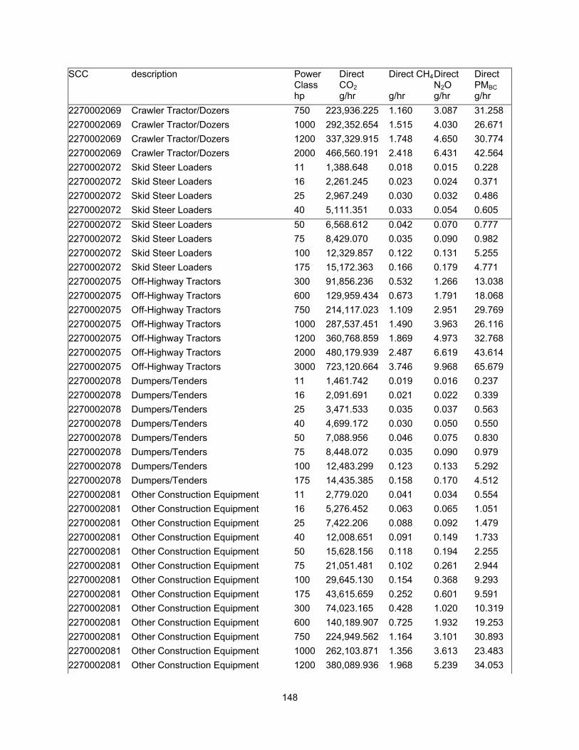
148
SCC description Power Class
Direct CO2
Direct CH4 Direct N2O
Direct PMBC
hp g/hr g/hr g/hr g/hr 2270002069 Crawler Tractor/Dozers 750 223,936.225 1.160 3.087 31.258 2270002069 Crawler Tractor/Dozers 1000 292,352.654 1.515 4.030 26.671 2270002069 Crawler Tractor/Dozers 1200 337,329.915 1.748 4.650 30.774 2270002069 Crawler Tractor/Dozers 2000 466,560.191 2.418 6.431 42.564 2270002072 Skid Steer Loaders 11 1,388.648 0.018 0.015 0.228 2270002072 Skid Steer Loaders 16 2,261.245 0.023 0.024 0.371 2270002072 Skid Steer Loaders 25 2,967.249 0.030 0.032 0.486 2270002072 Skid Steer Loaders 40 5,111.351 0.033 0.054 0.605 2270002072 Skid Steer Loaders 50 6,568.612 0.042 0.070 0.777 2270002072 Skid Steer Loaders 75 8,429.070 0.035 0.090 0.982 2270002072 Skid Steer Loaders 100 12,329.857 0.122 0.131 5.255 2270002072 Skid Steer Loaders 175 15,172.363 0.166 0.179 4.771 2270002075 Off-Highway Tractors 300 91,856.236 0.532 1.266 13.038 2270002075 Off-Highway Tractors 600 129,959.434 0.673 1.791 18.068 2270002075 Off-Highway Tractors 750 214,117.023 1.109 2.951 29.769 2270002075 Off-Highway Tractors 1000 287,537.451 1.490 3.963 26.116 2270002075 Off-Highway Tractors 1200 360,768.859 1.869 4.973 32.768 2270002075 Off-Highway Tractors 2000 480,179.939 2.487 6.619 43.614 2270002075 Off-Highway Tractors 3000 723,120.664 3.746 9.968 65.679 2270002078 Dumpers/Tenders 11 1,461.742 0.019 0.016 0.237 2270002078 Dumpers/Tenders 16 2,091.691 0.021 0.022 0.339 2270002078 Dumpers/Tenders 25 3,471.533 0.035 0.037 0.563 2270002078 Dumpers/Tenders 40 4,699.172 0.030 0.050 0.550 2270002078 Dumpers/Tenders 50 7,088.956 0.046 0.075 0.830 2270002078 Dumpers/Tenders 75 8,448.072 0.035 0.090 0.979 2270002078 Dumpers/Tenders 100 12,483.299 0.123 0.133 5.292 2270002078 Dumpers/Tenders 175 14,435.385 0.158 0.170 4.512 2270002081 Other Construction Equipment 11 2,779.020 0.041 0.034 0.554 2270002081 Other Construction Equipment 16 5,276.452 0.063 0.065 1.051 2270002081 Other Construction Equipment 25 7,422.206 0.088 0.092 1.479 2270002081 Other Construction Equipment 40 12,008.651 0.091 0.149 1.733 2270002081 Other Construction Equipment 50 15,628.156 0.118 0.194 2.255 2270002081 Other Construction Equipment 75 21,051.481 0.102 0.261 2.944 2270002081 Other Construction Equipment 100 29,645.130 0.154 0.368 9.293 2270002081 Other Construction Equipment 175 43,615.659 0.252 0.601 9.591 2270002081 Other Construction Equipment 300 74,023.165 0.428 1.020 10.319 2270002081 Other Construction Equipment 600 140,189.907 0.725 1.932 19.253 2270002081 Other Construction Equipment 750 224,949.562 1.164 3.101 30.893 2270002081 Other Construction Equipment 1000 262,103.871 1.356 3.613 23.483 2270002081 Other Construction Equipment 1200 380,089.936 1.968 5.239 34.053

149
SCC description Power Class
Direct CO2
Direct CH4 Direct N2O
Direct PMBC
hp g/hr g/hr g/hr g/hr 2270003010 Aerial Lifts 11 1,169.394 0.015 0.012 0.188 2270003010 Aerial Lifts 16 1,926.521 0.019 0.020 0.310 2270003010 Aerial Lifts 25 3,161.648 0.032 0.034 0.509 2270003010 Aerial Lifts 40 4,830.717 0.031 0.051 0.562 2270003010 Aerial Lifts 50 6,644.610 0.043 0.071 0.773 2270003010 Aerial Lifts 75 8,836.856 0.037 0.094 1.020 2270003010 Aerial Lifts 100 12,258.209 0.121 0.130 5.176 2270003010 Aerial Lifts 175 14,869.647 0.163 0.176 4.628 2270003020 Forklifts 16 5,276.452 0.063 0.065 1.176 2270003020 Forklifts 25 8,794.090 0.105 0.109 1.960 2270003020 Forklifts 40 12,198.597 0.093 0.151 1.971 2270003020 Forklifts 50 16,539.143 0.126 0.205 2.673 2270003020 Forklifts 75 21,716.208 0.106 0.270 3.238 2270003020 Forklifts 100 30,067.193 0.157 0.373 10.034 2270003020 Forklifts 175 42,950.532 0.249 0.592 10.143 2270003020 Forklifts 300 69,778.776 0.405 0.962 10.507 2270003020 Forklifts 600 112,095.014 0.582 1.545 16.230 2270003030 Sweepers/Scrubbers 6 1,269.447 0.019 0.016 0.263 2270003030 Sweepers/Scrubbers 11 2,792.691 0.033 0.035 0.579 2270003030 Sweepers/Scrubbers 25 5,506.684 0.066 0.069 1.142 2270003030 Sweepers/Scrubbers 40 8,842.268 0.067 0.111 1.329 2270003030 Sweepers/Scrubbers 50 11,078.879 0.085 0.139 1.665 2270003030 Sweepers/Scrubbers 75 15,437.365 0.076 0.193 2.219 2270003030 Sweepers/Scrubbers 100 20,781.521 0.104 0.260 4.496 2270003030 Sweepers/Scrubbers 175 30,668.456 0.170 0.427 4.424 2270003030 Sweepers/Scrubbers 300 49,485.161 0.275 0.690 4.273 2270003030 Sweepers/Scrubbers 600 83,076.132 0.435 1.158 7.001 2270003040 Other General Industrial Eqp 6 1,108.736 0.017 0.014 0.224 2270003040 Other General Industrial Eqp 11 2,432.261 0.036 0.030 0.491 2270003040 Other General Industrial Eqp 16 3,483.251 0.042 0.044 0.704 2270003040 Other General Industrial Eqp 25 5,742.788 0.069 0.072 1.160 2270003040 Other General Industrial Eqp 40 8,245.679 0.063 0.103 1.207 2270003040 Other General Industrial Eqp 50 11,248.948 0.086 0.141 1.646 2270003040 Other General Industrial Eqp 75 15,564.307 0.076 0.195 2.204 2270003040 Other General Industrial Eqp 100 21,860.458 0.109 0.274 4.660 2270003040 Other General Industrial Eqp 175 29,777.895 0.165 0.415 4.219 2270003040 Other General Industrial Eqp 300 53,481.376 0.296 0.745 4.524 2270003040 Other General Industrial Eqp 600 88,922.141 0.465 1.239 7.389 2270003040 Other General Industrial Eqp 750 148,431.522 0.777 2.068 12.334 2270003050 Other Material Handling Eqp 40 5,437.302 0.035 0.058 0.633
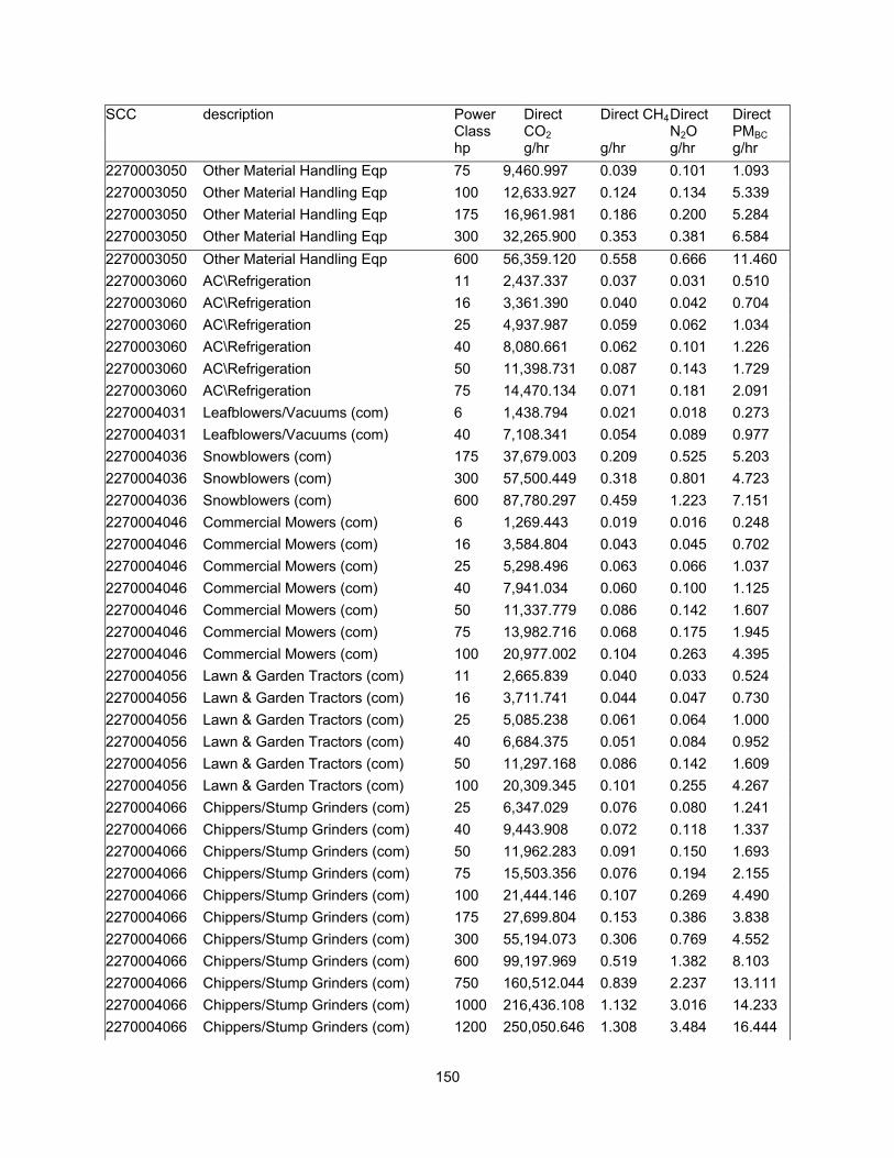
150
SCC description Power Class
Direct CO2
Direct CH4 Direct N2O
Direct PMBC
hp g/hr g/hr g/hr g/hr 2270003050 Other Material Handling Eqp 75 9,460.997 0.039 0.101 1.093 2270003050 Other Material Handling Eqp 100 12,633.927 0.124 0.134 5.339 2270003050 Other Material Handling Eqp 175 16,961.981 0.186 0.200 5.284 2270003050 Other Material Handling Eqp 300 32,265.900 0.353 0.381 6.584 2270003050 Other Material Handling Eqp 600 56,359.120 0.558 0.666 11.460 2270003060 AC\Refrigeration 11 2,437.337 0.037 0.031 0.510 2270003060 AC\Refrigeration 16 3,361.390 0.040 0.042 0.704 2270003060 AC\Refrigeration 25 4,937.987 0.059 0.062 1.034 2270003060 AC\Refrigeration 40 8,080.661 0.062 0.101 1.226 2270003060 AC\Refrigeration 50 11,398.731 0.087 0.143 1.729 2270003060 AC\Refrigeration 75 14,470.134 0.071 0.181 2.091 2270004031 Leafblowers/Vacuums (com) 6 1,438.794 0.021 0.018 0.273 2270004031 Leafblowers/Vacuums (com) 40 7,108.341 0.054 0.089 0.977 2270004036 Snowblowers (com) 175 37,679.003 0.209 0.525 5.203 2270004036 Snowblowers (com) 300 57,500.449 0.318 0.801 4.723 2270004036 Snowblowers (com) 600 87,780.297 0.459 1.223 7.151 2270004046 Commercial Mowers (com) 6 1,269.443 0.019 0.016 0.248 2270004046 Commercial Mowers (com) 16 3,584.804 0.043 0.045 0.702 2270004046 Commercial Mowers (com) 25 5,298.496 0.063 0.066 1.037 2270004046 Commercial Mowers (com) 40 7,941.034 0.060 0.100 1.125 2270004046 Commercial Mowers (com) 50 11,337.779 0.086 0.142 1.607 2270004046 Commercial Mowers (com) 75 13,982.716 0.068 0.175 1.945 2270004046 Commercial Mowers (com) 100 20,977.002 0.104 0.263 4.395 2270004056 Lawn & Garden Tractors (com) 11 2,665.839 0.040 0.033 0.524 2270004056 Lawn & Garden Tractors (com) 16 3,711.741 0.044 0.047 0.730 2270004056 Lawn & Garden Tractors (com) 25 5,085.238 0.061 0.064 1.000 2270004056 Lawn & Garden Tractors (com) 40 6,684.375 0.051 0.084 0.952 2270004056 Lawn & Garden Tractors (com) 50 11,297.168 0.086 0.142 1.609 2270004056 Lawn & Garden Tractors (com) 100 20,309.345 0.101 0.255 4.267 2270004066 Chippers/Stump Grinders (com) 25 6,347.029 0.076 0.080 1.241 2270004066 Chippers/Stump Grinders (com) 40 9,443.908 0.072 0.118 1.337 2270004066 Chippers/Stump Grinders (com) 50 11,962.283 0.091 0.150 1.693 2270004066 Chippers/Stump Grinders (com) 75 15,503.356 0.076 0.194 2.155 2270004066 Chippers/Stump Grinders (com) 100 21,444.146 0.107 0.269 4.490 2270004066 Chippers/Stump Grinders (com) 175 27,699.804 0.153 0.386 3.838 2270004066 Chippers/Stump Grinders (com) 300 55,194.073 0.306 0.769 4.552 2270004066 Chippers/Stump Grinders (com) 600 99,197.969 0.519 1.382 8.103 2270004066 Chippers/Stump Grinders (com) 750 160,512.044 0.839 2.237 13.111 2270004066 Chippers/Stump Grinders (com) 1000 216,436.108 1.132 3.016 14.233 2270004066 Chippers/Stump Grinders (com) 1200 250,050.646 1.308 3.484 16.444
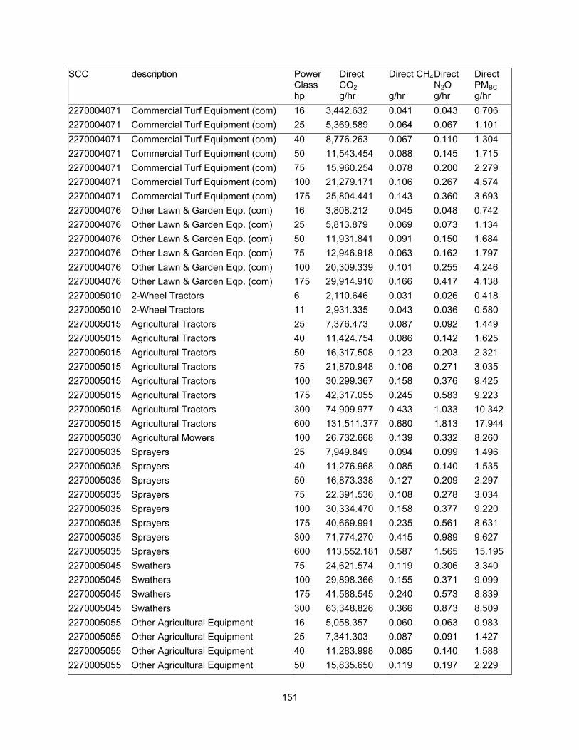
151
SCC description Power Class
Direct CO2
Direct CH4 Direct N2O
Direct PMBC
hp g/hr g/hr g/hr g/hr 2270004071 Commercial Turf Equipment (com) 16 3,442.632 0.041 0.043 0.706 2270004071 Commercial Turf Equipment (com) 25 5,369.589 0.064 0.067 1.101 2270004071 Commercial Turf Equipment (com) 40 8,776.263 0.067 0.110 1.304 2270004071 Commercial Turf Equipment (com) 50 11,543.454 0.088 0.145 1.715 2270004071 Commercial Turf Equipment (com) 75 15,960.254 0.078 0.200 2.279 2270004071 Commercial Turf Equipment (com) 100 21,279.171 0.106 0.267 4.574 2270004071 Commercial Turf Equipment (com) 175 25,804.441 0.143 0.360 3.693 2270004076 Other Lawn & Garden Eqp. (com) 16 3,808.212 0.045 0.048 0.742 2270004076 Other Lawn & Garden Eqp. (com) 25 5,813.879 0.069 0.073 1.134 2270004076 Other Lawn & Garden Eqp. (com) 50 11,931.841 0.091 0.150 1.684 2270004076 Other Lawn & Garden Eqp. (com) 75 12,946.918 0.063 0.162 1.797 2270004076 Other Lawn & Garden Eqp. (com) 100 20,309.339 0.101 0.255 4.246 2270004076 Other Lawn & Garden Eqp. (com) 175 29,914.910 0.166 0.417 4.138 2270005010 2-Wheel Tractors 6 2,110.646 0.031 0.026 0.418 2270005010 2-Wheel Tractors 11 2,931.335 0.043 0.036 0.580 2270005015 Agricultural Tractors 25 7,376.473 0.087 0.092 1.449 2270005015 Agricultural Tractors 40 11,424.754 0.086 0.142 1.625 2270005015 Agricultural Tractors 50 16,317.508 0.123 0.203 2.321 2270005015 Agricultural Tractors 75 21,870.948 0.106 0.271 3.035 2270005015 Agricultural Tractors 100 30,299.367 0.158 0.376 9.425 2270005015 Agricultural Tractors 175 42,317.055 0.245 0.583 9.223 2270005015 Agricultural Tractors 300 74,909.977 0.433 1.033 10.342 2270005015 Agricultural Tractors 600 131,511.377 0.680 1.813 17.944 2270005030 Agricultural Mowers 100 26,732.668 0.139 0.332 8.260 2270005035 Sprayers 25 7,949.849 0.094 0.099 1.496 2270005035 Sprayers 40 11,276.968 0.085 0.140 1.535 2270005035 Sprayers 50 16,873.338 0.127 0.209 2.297 2270005035 Sprayers 75 22,391.536 0.108 0.278 3.034 2270005035 Sprayers 100 30,334.470 0.158 0.377 9.220 2270005035 Sprayers 175 40,669.991 0.235 0.561 8.631 2270005035 Sprayers 300 71,774.270 0.415 0.989 9.627 2270005035 Sprayers 600 113,552.181 0.587 1.565 15.195 2270005045 Swathers 75 24,621.574 0.119 0.306 3.340 2270005045 Swathers 100 29,898.366 0.155 0.371 9.099 2270005045 Swathers 175 41,588.545 0.240 0.573 8.839 2270005045 Swathers 300 63,348.826 0.366 0.873 8.509 2270005055 Other Agricultural Equipment 16 5,058.357 0.060 0.063 0.983 2270005055 Other Agricultural Equipment 25 7,341.303 0.087 0.091 1.427 2270005055 Other Agricultural Equipment 40 11,283.998 0.085 0.140 1.588 2270005055 Other Agricultural Equipment 50 15,835.650 0.119 0.197 2.229

152
SCC description Power Class
Direct CO2
Direct CH4 Direct N2O
Direct PMBC
hp g/hr g/hr g/hr g/hr 2270005055 Other Agricultural Equipment 75 22,032.766 0.107 0.273 3.040 2270005055 Other Agricultural Equipment 100 29,880.777 0.156 0.371 9.243 2270005055 Other Agricultural Equipment 175 42,918.870 0.248 0.592 9.294 2270005055 Other Agricultural Equipment 300 72,977.838 0.422 1.006 10.005 2270005055 Other Agricultural Equipment 600 118,809.666 0.615 1.638 16.134 2270005060 Irrigation Sets 25 5,554.919 0.066 0.070 1.111 2270005060 Irrigation Sets 40 8,377.687 0.064 0.105 1.213 2270005060 Irrigation Sets 50 11,444.385 0.087 0.143 1.657 2270005060 Irrigation Sets 75 15,292.593 0.075 0.192 2.153 2270005060 Irrigation Sets 100 21,799.515 0.109 0.273 4.621 2270005060 Irrigation Sets 175 31,125.170 0.172 0.434 4.380 2270005060 Irrigation Sets 300 51,266.337 0.284 0.714 4.303 2270005060 Irrigation Sets 600 89,059.074 0.466 1.241 7.361 2270006005 Generator Sets 6 1,358.305 0.020 0.017 0.263 2270006005 Generator Sets 11 2,137.244 0.032 0.027 0.413 2270006005 Generator Sets 16 3,442.630 0.041 0.043 0.666 2270006005 Generator Sets 25 5,405.131 0.065 0.068 1.046 2270006005 Generator Sets 40 8,489.387 0.065 0.106 1.189 2270006005 Generator Sets 50 11,472.336 0.087 0.144 1.607 2270006005 Generator Sets 75 15,221.562 0.074 0.191 2.104 2270006005 Generator Sets 100 21,939.163 0.109 0.275 4.568 2270006005 Generator Sets 175 30,988.170 0.172 0.432 4.264 2270006005 Generator Sets 300 54,349.117 0.301 0.757 4.447 2270006005 Generator Sets 600 95,749.581 0.500 1.334 7.780 2270006010 Pumps 3 761.668 0.011 0.010 0.148 2270006010 Pumps 6 1,326.574 0.020 0.017 0.258 2270006010 Pumps 11 2,148.922 0.032 0.027 0.418 2270006010 Pumps 16 3,485.787 0.042 0.044 0.678 2270006010 Pumps 25 5,514.298 0.066 0.069 1.073 2270006010 Pumps 40 8,712.788 0.066 0.109 1.227 2270006010 Pumps 50 11,368.303 0.086 0.142 1.601 2270006010 Pumps 75 15,835.905 0.077 0.198 2.195 2270006010 Pumps 100 21,911.287 0.109 0.275 4.575 2270006010 Pumps 175 30,234.517 0.167 0.421 4.175 2270006010 Pumps 300 55,536.561 0.308 0.774 4.563 2270006010 Pumps 600 90,794.644 0.475 1.265 7.397 2270006015 Air Compressors 6 1,413.400 0.021 0.018 0.284 2270006015 Air Compressors 11 2,404.330 0.036 0.030 0.483 2270006015 Air Compressors 16 3,386.771 0.041 0.042 0.681 2270006015 Air Compressors 25 5,758.027 0.069 0.072 1.158

153
SCC description Power Class
Direct CO2
Direct CH4 Direct N2O
Direct PMBC
hp g/hr g/hr g/hr g/hr 2270006015 Air Compressors 40 8,504.618 0.065 0.107 1.238 2270006015 Air Compressors 50 11,236.222 0.086 0.141 1.636 2270006015 Air Compressors 75 15,424.636 0.075 0.193 2.178 2270006015 Air Compressors 100 21,289.328 0.106 0.267 4.526 2270006015 Air Compressors 175 29,503.782 0.163 0.411 4.166 2270006015 Air Compressors 300 55,559.424 0.308 0.774 4.682 2270006015 Air Compressors 600 97,599.631 0.511 1.360 8.089 2270006025 Welders 11 1,292.611 0.016 0.014 0.210 2270006025 Welders 16 2,145.775 0.022 0.023 0.349 2270006025 Welders 25 3,111.951 0.032 0.033 0.506 2270006025 Welders 40 4,820.492 0.031 0.051 0.566 2270006025 Welders 50 6,758.622 0.044 0.072 0.794 2270006025 Welders 75 9,393.719 0.039 0.100 1.090 2270006025 Welders 100 12,366.396 0.122 0.131 5.251 2270006025 Welders 175 19,975.332 0.219 0.236 6.255 2270006025 Welders 600 50,003.430 0.495 0.591 10.206 2270006030 Pressure Washers 6 1,315.148 0.020 0.016 0.250 2270006030 Pressure Washers 11 2,295.411 0.034 0.029 0.437 2270006030 Pressure Washers 16 3,546.720 0.042 0.044 0.675 2270006030 Pressure Washers 25 5,184.246 0.062 0.065 0.987 2270006030 Pressure Washers 40 7,928.339 0.060 0.099 1.093 2270006030 Pressure Washers 50 11,502.850 0.087 0.144 1.585 2270006030 Pressure Washers 75 15,571.906 0.076 0.195 2.134 2270006030 Pressure Washers 100 22,474.860 0.112 0.282 4.639 2270006030 Pressure Washers 175 29,298.281 0.162 0.408 3.989 2270006030 Pressure Washers 300 51,654.520 0.286 0.720 4.176 2270006030 Pressure Washers 600 94,882.234 0.496 1.322 7.646 2270006030 Pressure Washers 750 157,315.152 0.822 2.192 12.678 2270007015 Forest Eqp - Feller/Bunch/Skidde 40 12,476.495 0.095 0.155 1.933 2270007015 Forest Eqp - Feller/Bunch/Skidde 50 15,803.991 0.120 0.196 2.448 2270007015 Forest Eqp - Feller/Bunch/Skidde 75 22,894.539 0.111 0.284 3.332 2270007015 Forest Eqp - Feller/Bunch/Skidde 100 31,291.282 0.163 0.388 10.197 2270007015 Forest Eqp - Feller/Bunch/Skidde 175 43,393.975 0.252 0.598 9.975 2270007015 Forest Eqp - Feller/Bunch/Skidde 300 71,330.832 0.414 0.983 10.432 2270007015 Forest Eqp - Feller/Bunch/Skidde 600 133,443.322 0.692 1.839 18.935 2270007015 Forest Eqp - Feller/Bunch/Skidde 750 218,330.260 1.132 3.009 30.981 2285002015 Railway Maintenance 11 1,216.170 0.015 0.013 0.200 2285002015 Railway Maintenance 16 2,065.376 0.021 0.022 0.340 2285002015 Railway Maintenance 25 2,557.974 0.026 0.027 0.421 2285002015 Railway Maintenance 40 4,873.103 0.031 0.052 0.580

154
SCC description Power Class
Direct CO2
Direct CH4 Direct N2O
Direct PMBC
hp g/hr g/hr g/hr g/hr 2285002015 Railway Maintenance 50 6,448.758 0.042 0.069 0.767 2285002015 Railway Maintenance 75 8,712.623 0.036 0.093 1.018 2285002015 Railway Maintenance 100 12,840.029 0.127 0.137 5.487 2285002015 Railway Maintenance 175 17,633.052 0.193 0.208 5.561 2285002015 Railway Maintenance 300 30,792.010 0.337 0.364 6.365 2285002015 Railway Maintenance 600 59,635.661 0.591 0.704 12.232 2285002015 Railway Maintenance 750 90,690.427 0.898 1.071 18.602 2285004015 Railway Maintenance 3 3,943.624 2.782 0.014 0.294 2285004015 Railway Maintenance 6 4,559.598 3.265 0.016 0.345 2285004015 Railway Maintenance 11 7,669.532 2.404 0.030 0.154 2285004015 Railway Maintenance 16 13,627.690 4.403 0.055 0.281 2285004015 Railway Maintenance 25 20,662.826 5.976 0.083 0.382 2285004015 Railway Maintenance 40 14,974.695 0.519 0.152 0.497 2285006015 Railway Maintenance 40 11,338.917 0.172 0.152 0.451 2285002015 Railway Maintenance 750 90,690.427 0.898 1.071 18.602 2285004015 Railway Maintenance 3 3,943.624 2.782 0.014 0.294 2285004015 Railway Maintenance 6 4,559.598 3.265 0.016 0.345 2285004015 Railway Maintenance 11 7,669.532 2.404 0.030 0.154 2285004015 Railway Maintenance 16 13,627.690 4.403 0.055 0.281 2285004015 Railway Maintenance 25 20,662.826 5.976 0.083 0.382 2285004015 Railway Maintenance 40 14,974.695 0.519 0.152 0.497 2285006015 Railway Maintenance 40 11,338.917 0.172 0.152 0.451

155
Table 31. Upstream Emissions – 2010
SCC Description Power Class
Upstream CO2
Upstream CH4
Upstream N2O
Upstream PMBC
hp g/hr g/hr g/hr g/hr 2260002006 Tampers/Rammers 6 744.924 4.546 0.011 0.023 2260002009 Plate Compactors 3 442.863 2.703 0.007 0.014 2260002021 Paving Equipment 3 489.593 2.988 0.007 0.015 2260002027 Signal Boards/Light Plants 3 590.842 3.606 0.009 0.018 2260002039 Concrete/Industrial Saws 3 509.467 3.109 0.008 0.016 2260002039 Concrete/Industrial Saws 6 900.265 5.494 0.014 0.028 2260002054 Crushing/Proc. Equipment 3 483.416 2.950 0.007 0.015 2260003030 Sweepers/Scrubbers 3 342.689 2.091 0.005 0.010 2260003040 Other General Industrial Eqp 3 548.946 3.350 0.008 0.017 2260004016 Rotary Tillers < 6 HP (com) 1 257.016 1.569 0.004 0.008 2260004016 Rotary Tillers < 6 HP (com) 3 675.172 4.121 0.010 0.021 2260004021 Chain Saws < 6 HP (com) 3 566.671 3.458 0.009 0.017 2260004021 Chain Saws < 6 HP (com) 6 777.899 4.748 0.012 0.024 2260004026 Trimmers/Edgers/Brush Cutter (com) 3 375.991 2.295 0.006 0.012 2260004026 Trimmers/Edgers/Brush Cutter (com) 6 655.533 4.001 0.010 0.020 2260004031 Leafblowers/Vacuums (com) 3 378.676 2.311 0.006 0.012 2260004031 Leafblowers/Vacuums (com) 6 679.371 4.146 0.010 0.021 2260004036 Snowblowers (com) 3 784.477 4.788 0.012 0.024 2260004036 Snowblowers (com) 6 930.857 5.681 0.014 0.028 2260004071 Commercial Turf Equipment (com) 3 805.694 4.917 0.012 0.025 2260005035 Sprayers 1 236.337 1.442 0.004 0.007 2260005035 Sprayers 3 689.405 4.207 0.011 0.021 2260006005 Generator Sets 1 214.852 1.311 0.003 0.007 2260006005 Generator Sets 3 446.623 2.726 0.007 0.014 2260006010 Pumps 1 266.148 1.624 0.004 0.008 2260006010 Pumps 3 536.592 3.275 0.008 0.016 2260006010 Pumps 40 6,009.053 36.674 0.092 0.184 2260006010 Pumps 75 8,697.313 53.080 0.133 0.266 2260006015 Air Compressors 3 593.259 3.621 0.009 0.018 2260007005 Chain Saws > 6 HP 11 1,935.724 11.814 0.030 0.059 2265002003 Pavers 6 1,609.869 9.825 0.025 0.049 2265002003 Pavers 11 2,645.363 16.145 0.040 0.081 2265002003 Pavers 16 3,561.938 21.739 0.055 0.109 2265002003 Pavers 25 5,912.931 36.087 0.090 0.181 2265002003 Pavers 40 5,020.722 30.642 0.077 0.154 2265002003 Pavers 75 9,869.078 60.232 0.151 0.302 2265002006 Tampers/Rammers 11 2,132.058 13.012 0.033 0.065 2265002009 Plate Compactors 6 1,326.712 8.097 0.020 0.041

156
SCC Description Power Class
Upstream CO2
Upstream CH4
Upstream N2O
Upstream PMBC
hp g/hr g/hr g/hr g/hr 2265002009 Plate Compactors 11 2,332.559 14.236 0.036 0.071 2265002009 Plate Compactors 16 3,593.134 21.929 0.055 0.110 2265002015 Rollers 11 2,524.269 15.406 0.039 0.077 2265002015 Rollers 16 4,202.861 25.650 0.064 0.129 2265002015 Rollers 25 5,410.970 33.024 0.083 0.166 2265002015 Rollers 40 5,822.456 35.535 0.089 0.178 2265002015 Rollers 75 9,608.159 58.639 0.147 0.294 2265002015 Rollers 100 13,125.036 80.103 0.201 0.402 2265002021 Paving Equipment 6 1,545.474 9.432 0.024 0.047 2265002021 Paving Equipment 11 2,420.473 14.772 0.037 0.074 2265002021 Paving Equipment 16 3,760.454 22.950 0.058 0.115 2265002021 Paving Equipment 25 5,671.877 34.616 0.087 0.174 2265002021 Paving Equipment 40 5,787.666 35.323 0.089 0.177 2265002021 Paving Equipment 75 10,436.776 63.696 0.160 0.319 2265002024 Surfacing Equipment 6 1,552.696 9.476 0.024 0.048 2265002024 Surfacing Equipment 11 2,529.090 15.435 0.039 0.077 2265002024 Surfacing Equipment 16 4,426.900 27.018 0.068 0.135 2265002024 Surfacing Equipment 25 5,402.462 32.972 0.083 0.165 2265002024 Surfacing Equipment 40 4,781.941 29.185 0.073 0.146 2265002024 Surfacing Equipment 75 10,436.776 63.696 0.160 0.319 2265002027 Signal Boards/Light Plants 6 1,514.179 9.241 0.023 0.046 2265002027 Signal Boards/Light Plants 11 2,339.649 14.279 0.036 0.072 2265002027 Signal Boards/Light Plants 25 5,104.689 31.154 0.078 0.156 2265002030 Trenchers 3 850.781 5.192 0.013 0.026 2265002030 Trenchers 6 1,568.042 9.570 0.024 0.048 2265002030 Trenchers 11 2,519.164 15.375 0.039 0.077 2265002030 Trenchers 16 3,811.501 23.262 0.058 0.117 2265002030 Trenchers 25 5,473.361 33.404 0.084 0.168 2265002030 Trenchers 40 4,743.989 28.953 0.073 0.145 2265002030 Trenchers 75 9,755.223 59.537 0.149 0.299 2265002030 Trenchers 100 12,650.637 77.208 0.194 0.387 2265002033 Bore/Drill Rigs 1 255.234 1.558 0.004 0.008 2265002033 Bore/Drill Rigs 3 626.459 3.823 0.010 0.019 2265002033 Bore/Drill Rigs 6 1,447.076 8.832 0.022 0.044 2265002033 Bore/Drill Rigs 11 2,482.580 15.151 0.038 0.076 2265002033 Bore/Drill Rigs 16 4,537.501 27.693 0.069 0.139 2265002033 Bore/Drill Rigs 25 6,043.384 36.883 0.092 0.185 2265002033 Bore/Drill Rigs 40 4,963.794 30.294 0.076 0.152 2265002033 Bore/Drill Rigs 75 9,699.876 59.199 0.148 0.297 2265002033 Bore/Drill Rigs 175 18,675.503 113.978 0.286 0.572

157
SCC Description Power Class
Upstream CO2
Upstream CH4
Upstream N2O
Upstream PMBC
hp g/hr g/hr g/hr g/hr 2265002039 Concrete/Industrial Saws 11 2,420.473 14.772 0.037 0.074 2265002039 Concrete/Industrial Saws 16 4,163.157 25.408 0.064 0.127 2265002039 Concrete/Industrial Saws 25 5,504.556 33.595 0.084 0.168 2265002039 Concrete/Industrial Saws 40 5,501.446 33.576 0.084 0.168 2265002039 Concrete/Industrial Saws 75 10,401.986 63.484 0.159 0.318 2265002042 Cement & Mortar Mixers 3 819.586 5.002 0.013 0.025 2265002042 Cement & Mortar Mixers 6 1,570.750 9.586 0.024 0.048 2265002042 Cement & Mortar Mixers 11 2,374.531 14.492 0.036 0.073 2265002042 Cement & Mortar Mixers 16 3,834.189 23.400 0.059 0.117 2265002042 Cement & Mortar Mixers 25 5,067.822 30.929 0.078 0.155 2265002045 Cranes 11 2,268.751 13.846 0.035 0.069 2265002045 Cranes 16 3,975.985 24.266 0.061 0.122 2265002045 Cranes 25 5,150.064 31.431 0.079 0.158 2265002045 Cranes 40 5,850.920 35.709 0.090 0.179 2265002045 Cranes 75 10,917.500 66.630 0.167 0.334 2265002045 Cranes 175 18,216.917 111.179 0.279 0.558 2265002054 Crushing/Proc. Equipment 6 1,300.232 7.935 0.020 0.040 2265002054 Crushing/Proc. Equipment 11 2,532.493 15.456 0.039 0.078 2265002054 Crushing/Proc. Equipment 16 4,537.501 27.693 0.069 0.139 2265002054 Crushing/Proc. Equipment 75 9,888.054 60.347 0.151 0.303 2265002057 Rough Terrain Forklift 25 6,522.658 39.808 0.100 0.200 2265002057 Rough Terrain Forklift 40 4,585.856 27.988 0.070 0.140 2265002057 Rough Terrain Forklift 75 10,420.962 63.600 0.159 0.319 2265002057 Rough Terrain Forklift 100 12,650.637 77.208 0.194 0.387 2265002057 Rough Terrain Forklift 175 17,916.465 109.345 0.274 0.548 2265002060 Rubber Tire Loaders 40 5,850.920 35.709 0.090 0.179 2265002060 Rubber Tire Loaders 75 11,132.561 67.943 0.170 0.341 2265002060 Rubber Tire Loaders 175 17,869.025 109.056 0.273 0.547 2265002066 Tractors/Loaders/Backhoes 11 3,062.813 18.693 0.047 0.094 2265002066 Tractors/Loaders/Backhoes 25 5,410.970 33.024 0.083 0.166 2265002066 Tractors/Loaders/Backhoes 40 4,743.989 28.953 0.073 0.145 2265002066 Tractors/Loaders/Backhoes 75 9,646.111 58.871 0.148 0.295 2265002066 Tractors/Loaders/Backhoes 100 12,650.637 77.208 0.194 0.387 2265002072 Skid Steer Loaders 16 4,517.650 27.572 0.069 0.138 2265002072 Skid Steer Loaders 25 5,220.962 31.864 0.080 0.160 2265002072 Skid Steer Loaders 40 5,049.186 30.816 0.077 0.155 2265002072 Skid Steer Loaders 75 8,608.759 52.540 0.132 0.263 2265002072 Skid Steer Loaders 100 12,492.504 76.243 0.191 0.382 2265002078 Dumpers/Tenders 6 1,492.514 9.109 0.023 0.046 2265002078 Dumpers/Tenders 11 2,416.219 14.746 0.037 0.074

158
SCC Description Power Class
Upstream CO2
Upstream CH4
Upstream N2O
Upstream PMBC
hp g/hr g/hr g/hr g/hr 2265002078 Dumpers/Tenders 16 3,482.532 21.254 0.053 0.107 2265002078 Dumpers/Tenders 25 5,314.548 32.435 0.081 0.163 2265002078 Dumpers/Tenders 75 10,436.776 63.696 0.160 0.319 2265002081 Other Construction Equipment 25 5,104.689 31.154 0.078 0.156 2265002081 Other Construction Equipment 175 19,924.753 121.602 0.305 0.610 2265003010 Aerial Lifts 11 2,290.020 13.976 0.035 0.070 2265003010 Aerial Lifts 16 4,080.915 24.906 0.062 0.125 2265003010 Aerial Lifts 25 5,992.338 36.572 0.092 0.183 2265003010 Aerial Lifts 40 4,936.911 30.130 0.076 0.151 2265003010 Aerial Lifts 75 9,465.839 57.771 0.145 0.290 2265003010 Aerial Lifts 175 17,631.825 107.608 0.270 0.540 2265003020 Forklifts 40 5,711.763 34.859 0.087 0.175 2265003020 Forklifts 50 7,141.285 43.584 0.109 0.219 2265003020 Forklifts 75 9,926.006 60.579 0.152 0.304 2265003020 Forklifts 100 14,078.578 85.922 0.215 0.431 2265003020 Forklifts 175 22,881.840 139.649 0.350 0.700 2265003020 Forklifts 300 34,125.094 208.268 0.522 1.044 2265003030 Sweepers/Scrubbers 6 1,424.809 8.696 0.022 0.044 2265003030 Sweepers/Scrubbers 11 2,794.817 17.057 0.043 0.086 2265003030 Sweepers/Scrubbers 16 4,211.368 25.702 0.064 0.129 2265003030 Sweepers/Scrubbers 25 5,169.915 31.552 0.079 0.158 2265003030 Sweepers/Scrubbers 40 5,046.023 30.796 0.077 0.154 2265003030 Sweepers/Scrubbers 50 7,274.116 44.394 0.111 0.223 2265003030 Sweepers/Scrubbers 75 10,017.723 61.139 0.153 0.307 2265003030 Sweepers/Scrubbers 100 14,231.967 86.859 0.218 0.436 2265003030 Sweepers/Scrubbers 175 23,719.945 144.764 0.363 0.726 2265003030 Sweepers/Scrubbers 600 64,992.648 396.654 0.995 1.989 2265003040 Other General Industrial Eqp 6 1,290.603 7.877 0.020 0.040 2265003040 Other General Industrial Eqp 11 2,570.211 15.686 0.039 0.079 2265003040 Other General Industrial Eqp 16 3,837.024 23.418 0.059 0.117 2265003040 Other General Industrial Eqp 25 5,172.751 31.570 0.079 0.158 2265003040 Other General Industrial Eqp 40 4,762.965 29.069 0.073 0.146 2265003040 Other General Industrial Eqp 75 9,639.785 58.832 0.148 0.295 2265003040 Other General Industrial Eqp 100 12,650.637 77.208 0.194 0.387 2265003040 Other General Industrial Eqp 175 21,506.083 131.253 0.329 0.658 2265003040 Other General Industrial Eqp 300 30,835.928 188.194 0.472 0.944 2265003050 Other Material Handling Eqp 3 850.781 5.192 0.013 0.026 2265003050 Other Material Handling Eqp 25 5,138.720 31.362 0.079 0.157 2265003050 Other Material Handling Eqp 75 9,962.377 60.801 0.152 0.305 2265003050 Other Material Handling Eqp 100 13,599.435 82.998 0.208 0.416
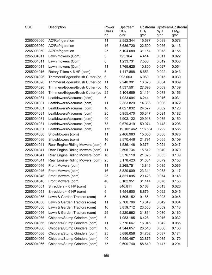
159
SCC Description Power Class
Upstream CO2
Upstream CH4
Upstream N2O
Upstream PMBC
hp g/hr g/hr g/hr g/hr 2265003060 AC\Refrigeration 11 2,552.344 15.577 0.039 0.078 2265003060 AC\Refrigeration 16 3,686.720 22.500 0.056 0.113 2265003060 AC\Refrigeration 25 5,104.689 31.154 0.078 0.156 2265004011 Lawn mowers (Com) 3 723.164 4.414 0.011 0.022 2265004011 Lawn mowers (Com) 6 1,233.731 7.530 0.019 0.038 2265004011 Lawn mowers (Com) 11 1,769.625 10.800 0.027 0.054 2265004016 Rotary Tillers < 6 HP (com) 6 1,417.888 8.653 0.022 0.043 2265004026 Trimmers/Edgers/Brush Cutter (co 6 993.003 6.060 0.015 0.030 2265004026 Trimmers/Edgers/Brush Cutter (co 11 2,240.391 13.673 0.034 0.069 2265004026 Trimmers/Edgers/Brush Cutter (co 16 4,537.501 27.693 0.069 0.139 2265004026 Trimmers/Edgers/Brush Cutter (co 25 5,104.689 31.154 0.078 0.156 2265004031 Leafblowers/Vacuums (com) 6 1,023.094 6.244 0.016 0.031 2265004031 Leafblowers/Vacuums (com) 11 2,353.829 14.366 0.036 0.072 2265004031 Leafblowers/Vacuums (com) 16 4,027.032 24.577 0.062 0.123 2265004031 Leafblowers/Vacuums (com) 25 5,955.470 36.347 0.091 0.182 2265004031 Leafblowers/Vacuums (com) 40 4,902.122 29.918 0.075 0.150 2265004031 Leafblowers/Vacuums (com) 75 9,679.319 59.074 0.148 0.296 2265004031 Leafblowers/Vacuums (com) 175 19,102.462 116.584 0.292 0.585 2265004036 Snowblowers (com) 11 2,466.983 15.056 0.038 0.076 2265004036 Snowblowers (com) 16 3,570.446 21.791 0.055 0.109 2265004041 Rear Engine Riding Mowers (com) 6 1,536.146 9.375 0.024 0.047 2265004041 Rear Engine Riding Mowers (com) 11 2,595.734 15.842 0.040 0.079 2265004041 Rear Engine Riding Mowers (com) 16 3,576.118 21.825 0.055 0.109 2265004041 Rear Engine Riding Mowers (com) 25 5,178.423 31.604 0.079 0.158 2265004046 Front Mowers (com) 11 2,268.751 13.846 0.035 0.069 2265004046 Front Mowers (com) 16 3,820.009 23.314 0.058 0.117 2265004046 Front Mowers (com) 25 4,821.095 29.423 0.074 0.148 2265004046 Front Mowers (com) 40 5,102.951 31.144 0.078 0.156 2265004051 Shredders < 6 HP (com) 3 846.811 5.168 0.013 0.026 2265004051 Shredders < 6 HP (com) 6 1,454.900 8.879 0.022 0.045 2265004056 Lawn & Garden Tractors (com) 6 1,505.152 9.186 0.023 0.046 2265004056 Lawn & Garden Tractors (com) 11 2,760.786 16.849 0.042 0.084 2265004056 Lawn & Garden Tractors (com) 16 3,859.712 23.556 0.059 0.118 2265004056 Lawn & Garden Tractors (com) 25 5,220.962 31.864 0.080 0.160 2265004066 Chippers/Stump Grinders (com) 6 1,053.185 6.428 0.016 0.032 2265004066 Chippers/Stump Grinders (com) 11 2,776.667 16.946 0.042 0.085 2265004066 Chippers/Stump Grinders (com) 16 4,344.657 26.516 0.066 0.133 2265004066 Chippers/Stump Grinders (com) 25 5,686.056 34.702 0.087 0.174 2265004066 Chippers/Stump Grinders (com) 40 5,550.467 33.875 0.085 0.170 2265004066 Chippers/Stump Grinders (com) 75 9,609.740 58.649 0.147 0.294
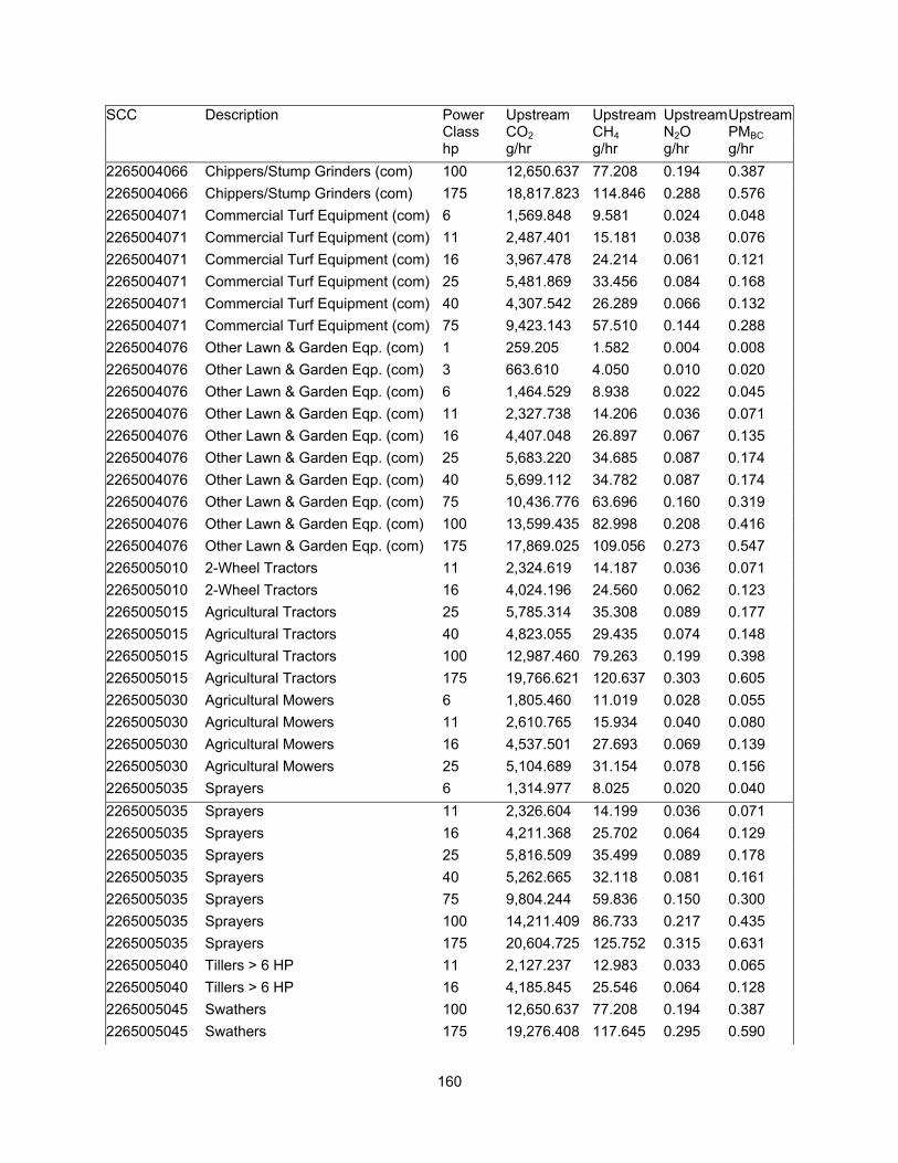
160
SCC Description Power Class
Upstream CO2
Upstream CH4
Upstream N2O
Upstream PMBC
hp g/hr g/hr g/hr g/hr 2265004066 Chippers/Stump Grinders (com) 100 12,650.637 77.208 0.194 0.387 2265004066 Chippers/Stump Grinders (com) 175 18,817.823 114.846 0.288 0.576 2265004071 Commercial Turf Equipment (com) 6 1,569.848 9.581 0.024 0.048 2265004071 Commercial Turf Equipment (com) 11 2,487.401 15.181 0.038 0.076 2265004071 Commercial Turf Equipment (com) 16 3,967.478 24.214 0.061 0.121 2265004071 Commercial Turf Equipment (com) 25 5,481.869 33.456 0.084 0.168 2265004071 Commercial Turf Equipment (com) 40 4,307.542 26.289 0.066 0.132 2265004071 Commercial Turf Equipment (com) 75 9,423.143 57.510 0.144 0.288 2265004076 Other Lawn & Garden Eqp. (com) 1 259.205 1.582 0.004 0.008 2265004076 Other Lawn & Garden Eqp. (com) 3 663.610 4.050 0.010 0.020 2265004076 Other Lawn & Garden Eqp. (com) 6 1,464.529 8.938 0.022 0.045 2265004076 Other Lawn & Garden Eqp. (com) 11 2,327.738 14.206 0.036 0.071 2265004076 Other Lawn & Garden Eqp. (com) 16 4,407.048 26.897 0.067 0.135 2265004076 Other Lawn & Garden Eqp. (com) 25 5,683.220 34.685 0.087 0.174 2265004076 Other Lawn & Garden Eqp. (com) 40 5,699.112 34.782 0.087 0.174 2265004076 Other Lawn & Garden Eqp. (com) 75 10,436.776 63.696 0.160 0.319 2265004076 Other Lawn & Garden Eqp. (com) 100 13,599.435 82.998 0.208 0.416 2265004076 Other Lawn & Garden Eqp. (com) 175 17,869.025 109.056 0.273 0.547 2265005010 2-Wheel Tractors 11 2,324.619 14.187 0.036 0.071 2265005010 2-Wheel Tractors 16 4,024.196 24.560 0.062 0.123 2265005015 Agricultural Tractors 25 5,785.314 35.308 0.089 0.177 2265005015 Agricultural Tractors 40 4,823.055 29.435 0.074 0.148 2265005015 Agricultural Tractors 100 12,987.460 79.263 0.199 0.398 2265005015 Agricultural Tractors 175 19,766.621 120.637 0.303 0.605 2265005030 Agricultural Mowers 6 1,805.460 11.019 0.028 0.055 2265005030 Agricultural Mowers 11 2,610.765 15.934 0.040 0.080 2265005030 Agricultural Mowers 16 4,537.501 27.693 0.069 0.139 2265005030 Agricultural Mowers 25 5,104.689 31.154 0.078 0.156 2265005035 Sprayers 6 1,314.977 8.025 0.020 0.040 2265005035 Sprayers 11 2,326.604 14.199 0.036 0.071 2265005035 Sprayers 16 4,211.368 25.702 0.064 0.129 2265005035 Sprayers 25 5,816.509 35.499 0.089 0.178 2265005035 Sprayers 40 5,262.665 32.118 0.081 0.161 2265005035 Sprayers 75 9,804.244 59.836 0.150 0.300 2265005035 Sprayers 100 14,211.409 86.733 0.217 0.435 2265005035 Sprayers 175 20,604.725 125.752 0.315 0.631 2265005040 Tillers > 6 HP 11 2,127.237 12.983 0.033 0.065 2265005040 Tillers > 6 HP 16 4,185.845 25.546 0.064 0.128 2265005045 Swathers 100 12,650.637 77.208 0.194 0.387 2265005045 Swathers 175 19,276.408 117.645 0.295 0.590

161
SCC Description Power Class
Upstream CO2
Upstream CH4
Upstream N2O
Upstream PMBC
hp g/hr g/hr g/hr g/hr 2265005055 Other Agricultural Equipment 6 1,456.405 8.889 0.022 0.045 2265005055 Other Agricultural Equipment 11 2,592.048 15.819 0.040 0.079 2265005055 Other Agricultural Equipment 16 4,001.509 24.421 0.061 0.122 2265005055 Other Agricultural Equipment 25 5,286.189 32.262 0.081 0.162 2265005055 Other Agricultural Equipment 40 5,096.625 31.105 0.078 0.156 2265005055 Other Agricultural Equipment 75 9,864.334 60.203 0.151 0.302 2265005055 Other Agricultural Equipment 100 13,922.026 84.967 0.213 0.426 2265005055 Other Agricultural Equipment 175 26,471.458 161.557 0.405 0.810 2265005055 Other Agricultural Equipment 300 36,386.395 222.069 0.557 1.114 2265005060 Irrigation Sets 6 1,411.870 8.617 0.022 0.043 2265005060 Irrigation Sets 11 2,529.090 15.435 0.039 0.077 2265005060 Irrigation Sets 75 9,440.538 57.616 0.144 0.289 2265005060 Irrigation Sets 100 12,690.170 77.449 0.194 0.388 2265005060 Irrigation Sets 175 19,055.022 116.294 0.292 0.583 2265005060 Irrigation Sets 300 33,239.549 202.863 0.509 1.017 2265006005 Generator Sets 6 1,374.256 8.387 0.021 0.042 2265006005 Generator Sets 11 2,500.163 15.259 0.038 0.077 2265006005 Generator Sets 16 4,066.735 24.820 0.062 0.124 2265006005 Generator Sets 25 5,876.064 35.862 0.090 0.180 2265006010 Pumps 6 1,393.514 8.505 0.021 0.043 2265006010 Pumps 11 2,364.322 14.430 0.036 0.072 2265006010 Pumps 16 4,200.025 25.633 0.064 0.129 2265006010 Pumps 25 5,203.947 31.760 0.080 0.159 2265006010 Pumps 40 5,052.348 30.835 0.077 0.155 2265006010 Pumps 50 7,274.116 44.394 0.111 0.223 2265006010 Pumps 75 9,582.858 58.485 0.147 0.293 2265006010 Pumps 100 12,848.303 78.414 0.197 0.393 2265006010 Pumps 175 18,232.731 111.276 0.279 0.558 2265006015 Air Compressors 6 1,561.121 9.528 0.024 0.048 2265006015 Air Compressors 11 2,814.669 17.178 0.043 0.086 2265006015 Air Compressors 16 3,865.384 23.591 0.059 0.118 2265006015 Air Compressors 25 5,294.697 32.314 0.081 0.162 2265006015 Air Compressors 40 5,008.071 30.565 0.077 0.153 2265006015 Air Compressors 75 9,603.415 58.610 0.147 0.294 2265006015 Air Compressors 100 12,917.882 78.839 0.198 0.395 2265006015 Air Compressors 175 20,857.738 127.296 0.319 0.638 2265006025 Welders 6 1,797.637 10.971 0.028 0.055 2265006025 Welders 11 2,644.796 16.141 0.040 0.081 2265006025 Welders 16 4,455.259 27.191 0.068 0.136 2265006025 Welders 25 5,161.408 31.500 0.079 0.158

162
SCC Description Power Class
Upstream CO2
Upstream CH4
Upstream N2O
Upstream PMBC
hp g/hr g/hr g/hr g/hr 2265006025 Welders 75 10,062.000 61.409 0.154 0.308 2265006025 Welders 100 12,650.637 77.208 0.194 0.387 2265006025 Welders 175 20,557.285 125.462 0.315 0.629 2265006030 Pressure Washers 3 850.781 5.192 0.013 0.026 2265006030 Pressure Washers 6 1,452.493 8.865 0.022 0.044 2265006030 Pressure Washers 11 2,581.838 15.757 0.040 0.079 2265006030 Pressure Washers 16 4,007.181 24.456 0.061 0.123 2265006030 Pressure Washers 25 5,331.564 32.539 0.082 0.163 2265006030 Pressure Washers 40 5,779.760 35.274 0.088 0.177 2265006030 Pressure Washers 75 10,436.776 63.696 0.160 0.319 2265007010 Shredders > 6 HP 11 2,301.931 14.049 0.035 0.070 2265007010 Shredders > 6 HP 16 3,578.954 21.843 0.055 0.110 2265007010 Shredders > 6 HP 25 5,830.689 35.585 0.089 0.178 2265007015 Forest Eqp - Feller/Bunch/Skidde 6 1,655.005 10.101 0.025 0.051 2265007015 Forest Eqp - Feller/Bunch/Skidde 11 2,552.344 15.577 0.039 0.078 2267002003 Pavers 40 2,374.959 29.777 0.039 0.052 2267002003 Pavers 75 4,668.383 58.532 0.076 0.101 2267002015 Rollers 40 2,754.204 34.532 0.045 0.060 2267002015 Rollers 75 4,544.960 56.984 0.074 0.099 2267002015 Rollers 100 6,208.553 77.842 0.101 0.135 2267002021 Paving Equipment 40 2,737.748 34.326 0.045 0.059 2267002021 Paving Equipment 75 4,936.922 61.899 0.080 0.107 2267002024 Surfacing Equipment 40 2,262.008 28.361 0.037 0.049 2267002024 Surfacing Equipment 75 4,936.922 61.899 0.080 0.107 2267002030 Trenchers 40 2,244.055 28.136 0.037 0.049 2267002030 Trenchers 75 4,614.526 57.857 0.075 0.100 2267002030 Trenchers 100 5,984.148 75.029 0.097 0.130 2267002033 Bore/Drill Rigs 40 2,348.030 29.439 0.038 0.051 2267002033 Bore/Drill Rigs 75 4,588.345 57.528 0.075 0.100 2267002033 Bore/Drill Rigs 175 8,834.098 110.761 0.144 0.192 2267002039 Concrete/Industrial Saws 40 2,602.356 32.628 0.042 0.056 2267002039 Concrete/Industrial Saws 75 4,920.465 61.692 0.080 0.107 2267002045 Cranes 40 2,767.668 34.701 0.045 0.060 2267002045 Cranes 75 5,164.319 64.750 0.084 0.112 2267002045 Cranes 175 8,617.173 108.041 0.140 0.187 2267002054 Crushing/Proc. Equipment 75 4,677.359 58.644 0.076 0.102 2267002057 Rough Terrain Forklift 40 2,169.254 27.198 0.035 0.047 2267002057 Rough Terrain Forklift 75 4,929.442 61.805 0.080 0.107 2267002057 Rough Terrain Forklift 100 5,984.148 75.029 0.097 0.130 2267002057 Rough Terrain Forklift 175 8,475.049 106.260 0.138 0.184

163
SCC Description Power Class
Upstream CO2
Upstream CH4
Upstream N2O
Upstream PMBC
hp g/hr g/hr g/hr g/hr 2267002060 Rubber Tire Loaders 40 2,767.668 34.701 0.045 0.060 2267002060 Rubber Tire Loaders 75 5,266.050 66.025 0.086 0.114 2267002060 Rubber Tire Loaders 175 8,452.609 105.978 0.138 0.184 2267002066 Tractors/Loaders/Backhoes 40 2,244.055 28.136 0.037 0.049 2267002066 Tractors/Loaders/Backhoes 75 4,562.913 57.209 0.074 0.099 2267002066 Tractors/Loaders/Backhoes 100 5,984.148 75.029 0.097 0.130 2267002072 Skid Steer Loaders 40 2,388.423 29.946 0.039 0.052 2267002072 Skid Steer Loaders 75 4,082.685 51.188 0.066 0.089 2267002072 Skid Steer Loaders 100 5,909.346 74.091 0.096 0.128 2267002081 Other Construction Equipment 175 9,425.033 118.170 0.153 0.205 2267003010 Aerial Lifts 40 2,335.314 29.280 0.038 0.051 2267003010 Aerial Lifts 75 4,479.135 56.159 0.073 0.097 2267003010 Aerial Lifts 175 8,340.406 104.571 0.136 0.181 2267003020 Forklifts 40 2,501.374 31.362 0.041 0.054 2267003020 Forklifts 50 3,398.248 42.607 0.055 0.074 2267003020 Forklifts 75 4,351.971 54.565 0.071 0.094 2267003020 Forklifts 100 5,971.431 74.869 0.097 0.130 2267003020 Forklifts 175 9,836.443 123.329 0.160 0.214 2267003020 Forklifts 300 16,142.238 202.390 0.263 0.350 2267003030 Sweepers/Scrubbers 40 2,318.857 29.074 0.038 0.050 2267003030 Sweepers/Scrubbers 50 3,515.687 44.079 0.057 0.076 2267003030 Sweepers/Scrubbers 75 4,738.697 59.413 0.077 0.103 2267003030 Sweepers/Scrubbers 100 6,732.166 84.407 0.110 0.146 2267003030 Sweepers/Scrubbers 175 11,220.277 140.679 0.183 0.244 2267003030 Sweepers/Scrubbers 600 30,743.559 385.460 0.501 0.667 2267003040 Other General Industrial Eqp 40 2,253.032 28.248 0.037 0.049 2267003040 Other General Industrial Eqp 75 4,559.921 57.172 0.074 0.099 2267003040 Other General Industrial Eqp 100 5,984.148 75.029 0.097 0.130 2267003040 Other General Industrial Eqp 175 10,173.051 127.549 0.166 0.221 2267003040 Other General Industrial Eqp 300 14,586.360 182.883 0.238 0.317 2267003050 Other Material Handling Eqp 75 4,009.379 50.269 0.065 0.087 2267003050 Other Material Handling Eqp 100 6,432.959 80.656 0.105 0.140 2267004066 Chippers/Stump Grinders (com) 40 2,625.545 32.919 0.043 0.057 2267004066 Chippers/Stump Grinders (com) 75 4,545.708 56.994 0.074 0.099 2267004066 Chippers/Stump Grinders (com) 100 5,984.148 75.029 0.097 0.130 2267004066 Chippers/Stump Grinders (com) 175 8,901.420 111.605 0.145 0.193 2267005055 Other Agricultural Equipment 175 11,519.484 144.430 0.188 0.250 2267006005 Generator Sets 40 2,267.992 28.436 0.037 0.049 2267006005 Generator Sets 50 3,440.137 43.132 0.056 0.075 2267006005 Generator Sets 75 4,705.784 59.001 0.077 0.102

164
SCC Description Power Class
Upstream CO2
Upstream CH4
Upstream N2O
Upstream PMBC
hp g/hr g/hr g/hr g/hr 2267006005 Generator Sets 100 6,079.894 76.229 0.099 0.132 2267006005 Generator Sets 175 10,382.496 130.175 0.169 0.225 2267006005 Generator Sets 300 17,922.522 224.711 0.292 0.389 2267006005 Generator Sets 600 27,826.287 348.884 0.453 0.604 2267006010 Pumps 40 2,389.919 29.965 0.039 0.052 2267006010 Pumps 50 3,440.885 43.142 0.056 0.075 2267006010 Pumps 75 4,263.705 53.458 0.069 0.093 2267006010 Pumps 100 6,077.650 76.201 0.099 0.132 2267006010 Pumps 175 8,624.653 108.135 0.140 0.187 2267006015 Air Compressors 40 2,368.974 29.702 0.039 0.051 2267006015 Air Compressors 75 4,542.716 56.956 0.074 0.099 2267006015 Air Compressors 100 6,110.563 76.614 0.099 0.133 2267006015 Air Compressors 175 9,866.363 123.704 0.161 0.214 2267006025 Welders 75 4,759.641 59.676 0.078 0.103 2267006025 Welders 100 5,984.148 75.029 0.097 0.130 2267006025 Welders 175 9,724.240 121.922 0.158 0.211 2267006030 Pressure Washers 40 2,734.007 34.279 0.045 0.059 2267006030 Pressure Washers 75 4,936.922 61.899 0.080 0.107 2268002081 Other Construction Equipment 175 13,381.301 90.290 0.213 0.426 2268003020 Forklifts 50 6,117.166 41.276 0.097 0.195 2268003030 Sweepers/Scrubbers 300 24,213.783 163.383 0.386 0.771 2268003040 Other General Industrial Eqp 100 12,552.935 84.701 0.200 0.400 2268003060 AC\Refrigeration 50 6,117.166 41.276 0.097 0.195 2268003060 AC\Refrigeration 75 9,430.631 63.633 0.150 0.300 2268006005 Generator Sets 40 4,043.702 27.285 0.064 0.129 2268006005 Generator Sets 50 6,075.111 40.992 0.097 0.194 2268006005 Generator Sets 75 7,702.532 51.973 0.123 0.245 2268006005 Generator Sets 100 12,159.142 82.044 0.194 0.387 2268006005 Generator Sets 175 18,835.774 127.094 0.300 0.600 2268006005 Generator Sets 300 30,560.343 206.206 0.487 0.974 2268006005 Generator Sets 600 50,033.322 337.600 0.797 1.594 2268006010 Pumps 40 4,078.111 27.517 0.065 0.130 2268006010 Pumps 75 6,626.930 44.715 0.106 0.211 2268006010 Pumps 175 22,302.169 150.484 0.355 0.711 2268006010 Pumps 300 31,350.477 211.537 0.499 0.999 2268006010 Pumps 600 53,945.760 363.999 0.859 1.719 2268006015 Air Compressors 75 6,626.930 44.715 0.106 0.211 2268006015 Air Compressors 175 18,861.263 127.266 0.300 0.601 2268006020 Gas Compressors 40 3,504.627 23.647 0.056 0.112 2268006020 Gas Compressors 50 5,765.429 38.902 0.092 0.184

165
SCC Description Power Class
Upstream CO2
Upstream CH4
Upstream N2O
Upstream PMBC
hp g/hr g/hr g/hr g/hr 2268006020 Gas Compressors 75 8,793.427 59.334 0.140 0.280 2268006020 Gas Compressors 100 11,622.616 78.424 0.185 0.370 2268006020 Gas Compressors 175 18,593.637 125.461 0.296 0.592 2268006020 Gas Compressors 300 30,853.457 208.184 0.491 0.983 2268006020 Gas Compressors 600 51,218.523 345.597 0.816 1.632 2270002003 Pavers 25 1,877.312 40.369 0.027 0.063 2270002003 Pavers 40 2,811.682 60.462 0.040 0.094 2270002003 Pavers 50 3,886.637 83.577 0.055 0.129 2270002003 Pavers 75 5,397.059 116.057 0.077 0.180 2270002003 Pavers 100 6,748.205 145.112 0.096 0.225 2270002003 Pavers 175 10,482.497 225.413 0.150 0.349 2270002003 Pavers 300 17,219.020 370.273 0.246 0.574 2270002003 Pavers 600 30,131.338 647.936 0.430 1.004 2270002006 Tampers/Rammers 6 360.033 7.742 0.005 0.012 2270002009 Plate Compactors 6 423.210 9.101 0.006 0.014 2270002009 Plate Compactors 11 733.266 15.768 0.010 0.024 2270002009 Plate Compactors 16 1,218.967 26.212 0.017 0.041 2270002009 Plate Compactors 25 1,744.443 37.512 0.025 0.058 2270002015 Rollers 6 466.156 10.024 0.007 0.016 2270002015 Rollers 11 745.353 16.028 0.011 0.025 2270002015 Rollers 16 1,161.533 24.977 0.017 0.039 2270002015 Rollers 25 1,687.009 36.277 0.024 0.056 2270002015 Rollers 40 2,787.680 59.946 0.040 0.093 2270002015 Rollers 50 3,926.926 84.444 0.056 0.131 2270002015 Rollers 75 5,206.756 111.965 0.074 0.173 2270002015 Rollers 100 6,601.014 141.947 0.094 0.220 2270002015 Rollers 175 10,295.588 221.394 0.147 0.343 2270002015 Rollers 300 16,899.717 363.407 0.241 0.563 2270002015 Rollers 600 32,748.069 704.206 0.468 1.091 2270002018 Scrapers 75 5,657.654 121.661 0.081 0.188 2270002018 Scrapers 175 12,522.924 269.290 0.179 0.417 2270002018 Scrapers 300 19,228.295 413.480 0.275 0.641 2270002018 Scrapers 600 32,903.826 707.555 0.470 1.096 2270002018 Scrapers 750 53,549.517 1,151.515 0.765 1.784 2270002018 Scrapers 1000 59,187.948 1,272.762 0.845 1.972 2270002021 Paving Equipment 6 396.036 8.516 0.006 0.013 2270002021 Paving Equipment 11 625.771 13.456 0.009 0.021 2270002021 Paving Equipment 16 1,260.114 27.097 0.018 0.042 2270002021 Paving Equipment 25 1,690.438 36.351 0.024 0.056 2270002021 Paving Equipment 40 2,899.119 62.342 0.041 0.097

166
SCC Description Power Class
Upstream CO2
Upstream CH4
Upstream N2O
Upstream PMBC
hp g/hr g/hr g/hr g/hr 2270002021 Paving Equipment 75 5,233.330 112.536 0.075 0.174 2270002021 Paving Equipment 100 6,481.859 139.384 0.093 0.216 2270002021 Paving Equipment 175 10,225.497 219.886 0.146 0.341 2270002021 Paving Equipment 300 17,927.718 385.513 0.256 0.597 2270002021 Paving Equipment 600 35,824.284 770.356 0.512 1.194 2270002024 Surfacing Equipment 11 574.338 12.350 0.008 0.019 2270002024 Surfacing Equipment 16 1,140.103 24.516 0.016 0.038 2270002024 Surfacing Equipment 25 1,856.739 39.927 0.027 0.062 2270002024 Surfacing Equipment 40 2,716.531 58.416 0.039 0.091 2270002024 Surfacing Equipment 50 3,848.919 82.766 0.055 0.128 2270002024 Surfacing Equipment 75 4,708.711 101.255 0.067 0.157 2270002024 Surfacing Equipment 100 6,300.401 135.482 0.090 0.210 2270002024 Surfacing Equipment 175 9,851.678 211.848 0.141 0.328 2270002024 Surfacing Equipment 300 18,145.779 390.202 0.259 0.605 2270002024 Surfacing Equipment 600 38,363.136 824.951 0.548 1.278 2270002024 Surfacing Equipment 750 55,566.580 1,194.889 0.793 1.851 2270002024 Surfacing Equipment 1000 69,857.354 1,502.194 0.997 2.327 2270002024 Surfacing Equipment 2000 120,244.990 2,585.717 1.717 4.006 2270002027 Signal Boards/Light Plants 6 462.899 9.954 0.007 0.015 2270002027 Signal Boards/Light Plants 11 666.489 14.332 0.010 0.022 2270002027 Signal Boards/Light Plants 16 1,176.963 25.309 0.017 0.039 2270002027 Signal Boards/Light Plants 25 1,901.315 40.885 0.027 0.063 2270002027 Signal Boards/Light Plants 40 2,599.092 55.890 0.037 0.087 2270002027 Signal Boards/Light Plants 50 3,617.469 77.789 0.052 0.121 2270002027 Signal Boards/Light Plants 75 5,081.602 109.273 0.073 0.169 2270002027 Signal Boards/Light Plants 100 6,862.594 147.571 0.098 0.229 2270002027 Signal Boards/Light Plants 175 12,144.479 261.152 0.173 0.405 2270002027 Signal Boards/Light Plants 300 16,655.285 358.151 0.238 0.555 2270002030 Trenchers 11 822.931 17.696 0.012 0.027 2270002030 Trenchers 16 1,328.691 28.572 0.019 0.044 2270002030 Trenchers 25 1,851.596 39.816 0.026 0.062 2270002030 Trenchers 40 2,923.121 62.858 0.042 0.097 2270002030 Trenchers 50 3,861.777 83.043 0.055 0.129 2270002030 Trenchers 75 5,230.758 112.481 0.075 0.174 2270002030 Trenchers 100 6,755.993 145.279 0.096 0.225 2270002030 Trenchers 175 10,459.133 224.911 0.149 0.348 2270002030 Trenchers 300 19,508.659 419.509 0.279 0.650 2270002030 Trenchers 600 32,288.583 694.325 0.461 1.076 2270002030 Trenchers 750 57,762.765 1,242.115 0.825 1.924 2270002030 Trenchers 2000 116,818.320 2,512.031 1.668 3.892

167
SCC Description Power Class
Upstream CO2
Upstream CH4
Upstream N2O
Upstream PMBC
hp g/hr g/hr g/hr g/hr 2270002033 Bore/Drill Rigs 11 685.776 14.747 0.010 0.023 2270002033 Bore/Drill Rigs 16 1,242.969 26.728 0.018 0.041 2270002033 Bore/Drill Rigs 25 2,012.753 43.282 0.029 0.067 2270002033 Bore/Drill Rigs 40 2,698.529 58.028 0.039 0.090 2270002033 Bore/Drill Rigs 50 3,851.491 82.821 0.055 0.128 2270002033 Bore/Drill Rigs 75 5,301.907 114.011 0.076 0.177 2270002033 Bore/Drill Rigs 100 6,563.416 141.138 0.094 0.219 2270002033 Bore/Drill Rigs 175 10,162.808 218.538 0.145 0.339 2270002033 Bore/Drill Rigs 300 18,444.186 396.619 0.263 0.615 2270002033 Bore/Drill Rigs 600 34,474.898 741.339 0.492 1.149 2270002033 Bore/Drill Rigs 750 53,242.937 1,144.922 0.760 1.774 2270002033 Bore/Drill Rigs 1000 67,006.679 1,440.894 0.957 2.232 2270002033 Bore/Drill Rigs 1200 80,963.191 1,741.011 1.156 2.697 2270002033 Bore/Drill Rigs 2000 115,661.700 2,487.159 1.652 3.854 2270002036 Excavators 6 514.332 11.060 0.007 0.017 2270002036 Excavators 11 682.947 14.686 0.010 0.023 2270002036 Excavators 16 1,126.387 24.222 0.016 0.038 2270002036 Excavators 25 1,846.452 39.706 0.026 0.062 2270002036 Excavators 40 2,833.113 60.923 0.040 0.094 2270002036 Excavators 50 3,923.497 84.370 0.056 0.131 2270002036 Excavators 75 5,254.760 112.997 0.075 0.175 2270002036 Excavators 100 7,139.157 153.519 0.102 0.238 2270002036 Excavators 175 10,716.134 230.437 0.153 0.357 2270002036 Excavators 300 18,169.142 390.705 0.259 0.605 2270002036 Excavators 600 31,977.068 687.627 0.457 1.065 2270002036 Excavators 750 56,026.066 1,204.770 0.800 1.867 2270002036 Excavators 1000 68,844.929 1,480.423 0.983 2.294 2270002036 Excavators 1200 93,454.655 2,009.624 1.334 3.114 2270002036 Excavators 2000 137,689.860 2,960.847 1.966 4.587 2270002036 Excavators 3000 183,015.370 3,935.515 2.613 6.098 2270002039 Concrete/Industrial Saws 11 857.220 18.433 0.012 0.029 2270002039 Concrete/Industrial Saws 25 1,724.727 37.088 0.025 0.057 2270002039 Concrete/Industrial Saws 40 2,823.684 60.720 0.040 0.094 2270002039 Concrete/Industrial Saws 50 3,703.191 79.632 0.053 0.123 2270002039 Concrete/Industrial Saws 75 4,959.019 106.638 0.071 0.165 2270002039 Concrete/Industrial Saws 100 6,344.792 136.437 0.091 0.211 2270002039 Concrete/Industrial Saws 175 9,415.557 202.470 0.134 0.314 2270002039 Concrete/Industrial Saws 300 18,807.749 404.437 0.269 0.627 2270002042 Cement & Mortar Mixers 6 512.875 11.029 0.007 0.017 2270002042 Cement & Mortar Mixers 11 692.805 14.898 0.010 0.023
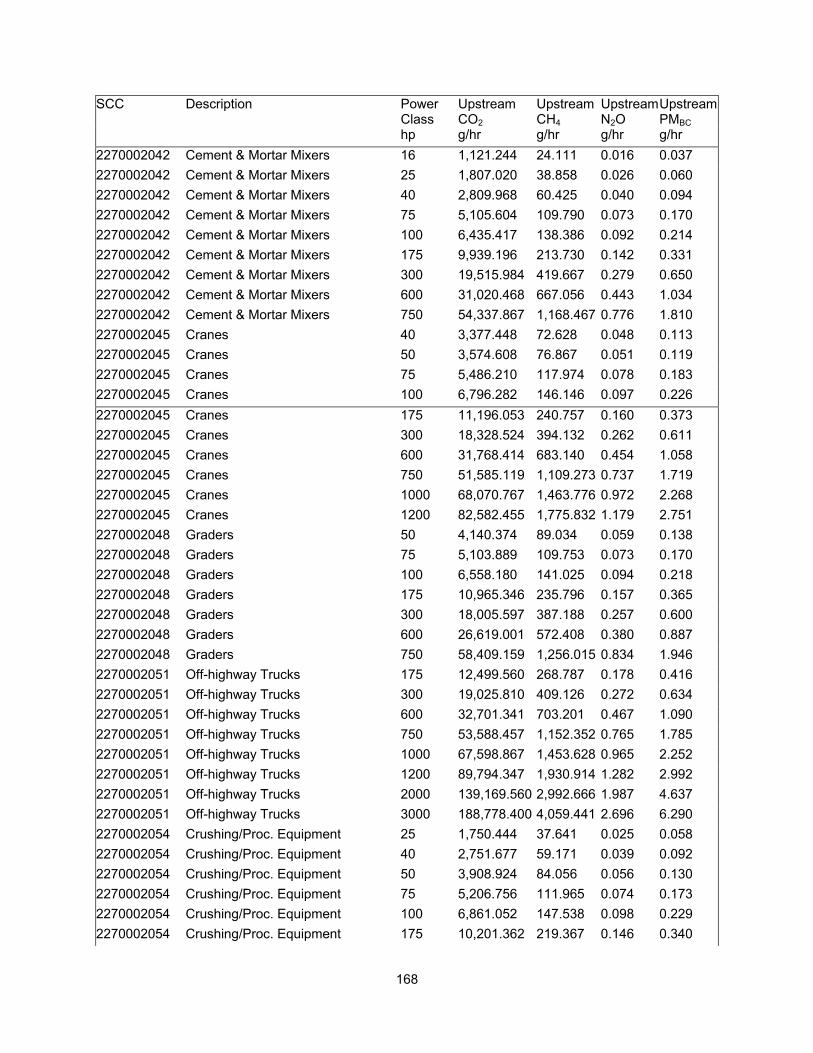
168
SCC Description Power Class
Upstream CO2
Upstream CH4
Upstream N2O
Upstream PMBC
hp g/hr g/hr g/hr g/hr 2270002042 Cement & Mortar Mixers 16 1,121.244 24.111 0.016 0.037 2270002042 Cement & Mortar Mixers 25 1,807.020 38.858 0.026 0.060 2270002042 Cement & Mortar Mixers 40 2,809.968 60.425 0.040 0.094 2270002042 Cement & Mortar Mixers 75 5,105.604 109.790 0.073 0.170 2270002042 Cement & Mortar Mixers 100 6,435.417 138.386 0.092 0.214 2270002042 Cement & Mortar Mixers 175 9,939.196 213.730 0.142 0.331 2270002042 Cement & Mortar Mixers 300 19,515.984 419.667 0.279 0.650 2270002042 Cement & Mortar Mixers 600 31,020.468 667.056 0.443 1.034 2270002042 Cement & Mortar Mixers 750 54,337.867 1,168.467 0.776 1.810 2270002045 Cranes 40 3,377.448 72.628 0.048 0.113 2270002045 Cranes 50 3,574.608 76.867 0.051 0.119 2270002045 Cranes 75 5,486.210 117.974 0.078 0.183 2270002045 Cranes 100 6,796.282 146.146 0.097 0.226 2270002045 Cranes 175 11,196.053 240.757 0.160 0.373 2270002045 Cranes 300 18,328.524 394.132 0.262 0.611 2270002045 Cranes 600 31,768.414 683.140 0.454 1.058 2270002045 Cranes 750 51,585.119 1,109.273 0.737 1.719 2270002045 Cranes 1000 68,070.767 1,463.776 0.972 2.268 2270002045 Cranes 1200 82,582.455 1,775.832 1.179 2.751 2270002048 Graders 50 4,140.374 89.034 0.059 0.138 2270002048 Graders 75 5,103.889 109.753 0.073 0.170 2270002048 Graders 100 6,558.180 141.025 0.094 0.218 2270002048 Graders 175 10,965.346 235.796 0.157 0.365 2270002048 Graders 300 18,005.597 387.188 0.257 0.600 2270002048 Graders 600 26,619.001 572.408 0.380 0.887 2270002048 Graders 750 58,409.159 1,256.015 0.834 1.946 2270002051 Off-highway Trucks 175 12,499.560 268.787 0.178 0.416 2270002051 Off-highway Trucks 300 19,025.810 409.126 0.272 0.634 2270002051 Off-highway Trucks 600 32,701.341 703.201 0.467 1.090 2270002051 Off-highway Trucks 750 53,588.457 1,152.352 0.765 1.785 2270002051 Off-highway Trucks 1000 67,598.867 1,453.628 0.965 2.252 2270002051 Off-highway Trucks 1200 89,794.347 1,930.914 1.282 2.992 2270002051 Off-highway Trucks 2000 139,169.560 2,992.666 1.987 4.637 2270002051 Off-highway Trucks 3000 188,778.400 4,059.441 2.696 6.290 2270002054 Crushing/Proc. Equipment 25 1,750.444 37.641 0.025 0.058 2270002054 Crushing/Proc. Equipment 40 2,751.677 59.171 0.039 0.092 2270002054 Crushing/Proc. Equipment 50 3,908.924 84.056 0.056 0.130 2270002054 Crushing/Proc. Equipment 75 5,206.756 111.965 0.074 0.173 2270002054 Crushing/Proc. Equipment 100 6,861.052 147.538 0.098 0.229 2270002054 Crushing/Proc. Equipment 175 10,201.362 219.367 0.146 0.340

169
SCC Description Power Class
Upstream CO2
Upstream CH4
Upstream N2O
Upstream PMBC
hp g/hr g/hr g/hr g/hr 2270002054 Crushing/Proc. Equipment 300 18,606.112 400.101 0.266 0.620 2270002054 Crushing/Proc. Equipment 600 32,632.021 701.711 0.466 1.087 2270002054 Crushing/Proc. Equipment 750 51,376.928 1,104.796 0.734 1.712 2270002054 Crushing/Proc. Equipment 1000 70,939.177 1,525.458 1.013 2.363 2270002057 Rough Terrain Forklifts 16 1,157.247 24.885 0.017 0.039 2270002057 Rough Terrain Forklifts 25 1,924.459 41.383 0.027 0.064 2270002057 Rough Terrain Forklifts 40 2,859.687 61.494 0.041 0.095 2270002057 Rough Terrain Forklifts 50 3,862.634 83.061 0.055 0.129 2270002057 Rough Terrain Forklifts 75 5,265.047 113.218 0.075 0.175 2270002057 Rough Terrain Forklifts 100 6,666.432 143.353 0.095 0.222 2270002057 Rough Terrain Forklifts 175 9,812.739 211.011 0.140 0.327 2270002057 Rough Terrain Forklifts 300 17,842.051 383.671 0.255 0.594 2270002057 Rough Terrain Forklifts 600 26,953.880 579.609 0.385 0.898 2270002060 Rubber Tire Loaders 25 1,957.034 42.084 0.028 0.065 2270002060 Rubber Tire Loaders 40 2,947.123 63.374 0.042 0.098 2270002060 Rubber Tire Loaders 50 3,895.209 83.762 0.056 0.130 2270002060 Rubber Tire Loaders 75 5,289.049 113.734 0.076 0.176 2270002060 Rubber Tire Loaders 100 6,657.087 143.152 0.095 0.222 2270002060 Rubber Tire Loaders 175 10,614.891 228.260 0.152 0.354 2270002060 Rubber Tire Loaders 300 17,912.142 385.178 0.256 0.597 2270002060 Rubber Tire Loaders 600 32,662.402 702.364 0.466 1.088 2270002060 Rubber Tire Loaders 750 53,907.760 1,159.218 0.770 1.796 2270002060 Rubber Tire Loaders 1000 67,466.473 1,450.781 0.963 2.248 2270002060 Rubber Tire Loaders 1200 84,264.947 1,812.011 1.203 2.807 2270002060 Rubber Tire Loaders 2000 145,399.870 3,126.641 2.076 4.844 2270002060 Rubber Tire Loaders 3000 174,682.330 3,756.323 2.494 5.820 2270002066 Tractors/Loaders/Backhoes 16 1,328.691 28.572 0.019 0.044 2270002066 Tractors/Loaders/Backhoes 25 1,952.748 41.991 0.028 0.065 2270002066 Tractors/Loaders/Backhoes 40 2,785.109 59.890 0.040 0.093 2270002066 Tractors/Loaders/Backhoes 50 3,962.929 85.218 0.057 0.132 2270002066 Tractors/Loaders/Backhoes 75 5,354.198 115.135 0.076 0.178 2270002066 Tractors/Loaders/Backhoes 100 7,931.355 170.554 0.113 0.264 2270002066 Tractors/Loaders/Backhoes 175 10,982.156 236.157 0.157 0.366 2270002066 Tractors/Loaders/Backhoes 300 18,197.441 391.313 0.260 0.606 2270002069 Crawler Tractor/Dozers 75 4,970.163 106.877 0.071 0.166 2270002069 Crawler Tractor/Dozers 100 6,842.438 147.138 0.098 0.228 2270002069 Crawler Tractor/Dozers 175 10,599.315 227.925 0.151 0.353 2270002069 Crawler Tractor/Dozers 300 18,340.476 394.389 0.262 0.611 2270002069 Crawler Tractor/Dozers 600 33,121.887 712.244 0.473 1.104 2270002069 Crawler Tractor/Dozers 750 55,060.367 1,184.004 0.786 1.834
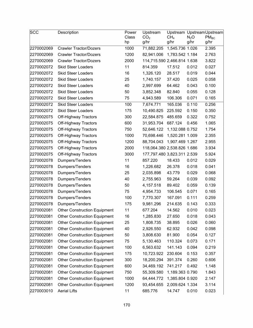
170
SCC Description Power Class
Upstream CO2
Upstream CH4
Upstream N2O
Upstream PMBC
hp g/hr g/hr g/hr g/hr 2270002069 Crawler Tractor/Dozers 1000 71,882.205 1,545.736 1.026 2.395 2270002069 Crawler Tractor/Dozers 1200 82,941.006 1,783.542 1.184 2.763 2270002069 Crawler Tractor/Dozers 2000 114,715.590 2,466.814 1.638 3.822 2270002072 Skid Steer Loaders 11 814.359 17.512 0.012 0.027 2270002072 Skid Steer Loaders 16 1,326.120 28.517 0.019 0.044 2270002072 Skid Steer Loaders 25 1,740.157 37.420 0.025 0.058 2270002072 Skid Steer Loaders 40 2,997.699 64.462 0.043 0.100 2270002072 Skid Steer Loaders 50 3,852.348 82.840 0.055 0.128 2270002072 Skid Steer Loaders 75 4,943.589 106.306 0.071 0.165 2270002072 Skid Steer Loaders 100 7,674.771 165.036 0.110 0.256 2270002072 Skid Steer Loaders 175 10,490.825 225.592 0.150 0.350 2270002075 Off-Highway Tractors 300 22,584.875 485.659 0.322 0.752 2270002075 Off-Highway Tractors 600 31,953.704 687.124 0.456 1.065 2270002075 Off-Highway Tractors 750 52,646.122 1,132.088 0.752 1.754 2270002075 Off-Highway Tractors 1000 70,698.446 1,520.281 1.009 2.355 2270002075 Off-Highway Tractors 1200 88,704.043 1,907.469 1.267 2.955 2270002075 Off-Highway Tractors 2000 118,064.380 2,538.826 1.686 3.934 2270002075 Off-Highway Tractors 3000 177,797.480 3,823.311 2.539 5.924 2270002078 Dumpers/Tenders 11 857.220 18.433 0.012 0.029 2270002078 Dumpers/Tenders 16 1,226.682 26.378 0.018 0.041 2270002078 Dumpers/Tenders 25 2,035.898 43.779 0.029 0.068 2270002078 Dumpers/Tenders 40 2,755.963 59.264 0.039 0.092 2270002078 Dumpers/Tenders 50 4,157.518 89.402 0.059 0.139 2270002078 Dumpers/Tenders 75 4,954.733 106.545 0.071 0.165 2270002078 Dumpers/Tenders 100 7,770.307 167.091 0.111 0.259 2270002078 Dumpers/Tenders 175 9,981.296 214.635 0.143 0.333 2270002081 Other Construction Equipment 11 677.204 14.562 0.010 0.023 2270002081 Other Construction Equipment 16 1,285.830 27.650 0.018 0.043 2270002081 Other Construction Equipment 25 1,808.735 38.895 0.026 0.060 2270002081 Other Construction Equipment 40 2,926.550 62.932 0.042 0.098 2270002081 Other Construction Equipment 50 3,808.630 81.900 0.054 0.127 2270002081 Other Construction Equipment 75 5,130.463 110.324 0.073 0.171 2270002081 Other Construction Equipment 100 6,563.632 141.143 0.094 0.219 2270002081 Other Construction Equipment 175 10,723.922 230.604 0.153 0.357 2270002081 Other Construction Equipment 300 18,200.294 391.374 0.260 0.606 2270002081 Other Construction Equipment 600 34,469.192 741.217 0.492 1.148 2270002081 Other Construction Equipment 750 55,309.580 1,189.363 0.790 1.843 2270002081 Other Construction Equipment 1000 64,444.772 1,385.804 0.920 2.147 2270002081 Other Construction Equipment 1200 93,454.655 2,009.624 1.334 3.114 2270003010 Aerial Lifts 11 685.776 14.747 0.010 0.023
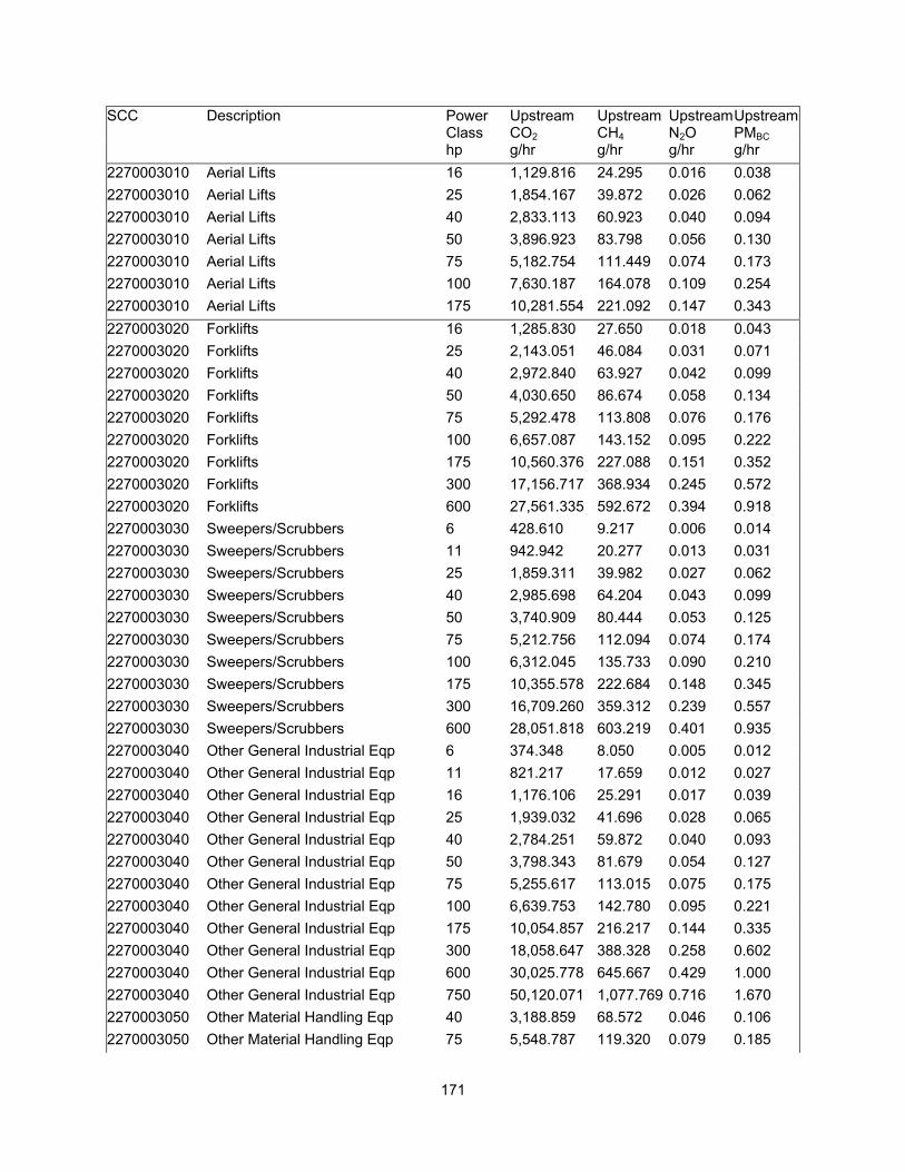
171
SCC Description Power Class
Upstream CO2
Upstream CH4
Upstream N2O
Upstream PMBC
hp g/hr g/hr g/hr g/hr 2270003010 Aerial Lifts 16 1,129.816 24.295 0.016 0.038 2270003010 Aerial Lifts 25 1,854.167 39.872 0.026 0.062 2270003010 Aerial Lifts 40 2,833.113 60.923 0.040 0.094 2270003010 Aerial Lifts 50 3,896.923 83.798 0.056 0.130 2270003010 Aerial Lifts 75 5,182.754 111.449 0.074 0.173 2270003010 Aerial Lifts 100 7,630.187 164.078 0.109 0.254 2270003010 Aerial Lifts 175 10,281.554 221.092 0.147 0.343 2270003020 Forklifts 16 1,285.830 27.650 0.018 0.043 2270003020 Forklifts 25 2,143.051 46.084 0.031 0.071 2270003020 Forklifts 40 2,972.840 63.927 0.042 0.099 2270003020 Forklifts 50 4,030.650 86.674 0.058 0.134 2270003020 Forklifts 75 5,292.478 113.808 0.076 0.176 2270003020 Forklifts 100 6,657.087 143.152 0.095 0.222 2270003020 Forklifts 175 10,560.376 227.088 0.151 0.352 2270003020 Forklifts 300 17,156.717 368.934 0.245 0.572 2270003020 Forklifts 600 27,561.335 592.672 0.394 0.918 2270003030 Sweepers/Scrubbers 6 428.610 9.217 0.006 0.014 2270003030 Sweepers/Scrubbers 11 942.942 20.277 0.013 0.031 2270003030 Sweepers/Scrubbers 25 1,859.311 39.982 0.027 0.062 2270003030 Sweepers/Scrubbers 40 2,985.698 64.204 0.043 0.099 2270003030 Sweepers/Scrubbers 50 3,740.909 80.444 0.053 0.125 2270003030 Sweepers/Scrubbers 75 5,212.756 112.094 0.074 0.174 2270003030 Sweepers/Scrubbers 100 6,312.045 135.733 0.090 0.210 2270003030 Sweepers/Scrubbers 175 10,355.578 222.684 0.148 0.345 2270003030 Sweepers/Scrubbers 300 16,709.260 359.312 0.239 0.557 2270003030 Sweepers/Scrubbers 600 28,051.818 603.219 0.401 0.935 2270003040 Other General Industrial Eqp 6 374.348 8.050 0.005 0.012 2270003040 Other General Industrial Eqp 11 821.217 17.659 0.012 0.027 2270003040 Other General Industrial Eqp 16 1,176.106 25.291 0.017 0.039 2270003040 Other General Industrial Eqp 25 1,939.032 41.696 0.028 0.065 2270003040 Other General Industrial Eqp 40 2,784.251 59.872 0.040 0.093 2270003040 Other General Industrial Eqp 50 3,798.343 81.679 0.054 0.127 2270003040 Other General Industrial Eqp 75 5,255.617 113.015 0.075 0.175 2270003040 Other General Industrial Eqp 100 6,639.753 142.780 0.095 0.221 2270003040 Other General Industrial Eqp 175 10,054.857 216.217 0.144 0.335 2270003040 Other General Industrial Eqp 300 18,058.647 388.328 0.258 0.602 2270003040 Other General Industrial Eqp 600 30,025.778 645.667 0.429 1.000 2270003040 Other General Industrial Eqp 750 50,120.071 1,077.769 0.716 1.670 2270003050 Other Material Handling Eqp 40 3,188.859 68.572 0.046 0.106 2270003050 Other Material Handling Eqp 75 5,548.787 119.320 0.079 0.185

172
SCC Description Power Class
Upstream CO2
Upstream CH4
Upstream N2O
Upstream PMBC
hp g/hr g/hr g/hr g/hr 2270003050 Other Material Handling Eqp 100 7,864.024 169.106 0.112 0.262 2270003050 Other Material Handling Eqp 175 11,728.251 252.201 0.167 0.391 2270003050 Other Material Handling Eqp 300 22,310.063 479.750 0.319 0.743 2270003050 Other Material Handling Eqp 600 38,969.820 837.997 0.556 1.298 2270003060 AC\Refrigeration 11 822.931 17.696 0.012 0.027 2270003060 AC\Refrigeration 16 1,134.960 24.406 0.016 0.038 2270003060 AC\Refrigeration 25 1,667.293 35.853 0.024 0.056 2270003060 AC\Refrigeration 40 2,728.532 58.674 0.039 0.091 2270003060 AC\Refrigeration 50 3,848.919 82.766 0.055 0.128 2270003060 AC\Refrigeration 75 4,886.155 105.071 0.070 0.163 2270004031 Leafblowers/Vacuums (com) 6 485.787 10.446 0.007 0.016 2270004031 Leafblowers/Vacuums (com) 40 2,400.217 51.614 0.034 0.080 2270004036 Snowblowers (com) 175 12,722.787 273.588 0.182 0.424 2270004036 Snowblowers (com) 300 19,415.744 417.511 0.277 0.647 2270004036 Snowblowers (com) 600 29,640.239 637.376 0.423 0.988 2270004046 Commercial Mowers (com) 6 428.610 9.217 0.006 0.014 2270004046 Commercial Mowers (com) 16 1,210.395 26.028 0.017 0.040 2270004046 Commercial Mowers (com) 25 1,789.019 38.471 0.026 0.060 2270004046 Commercial Mowers (com) 40 2,681.385 57.660 0.038 0.089 2270004046 Commercial Mowers (com) 50 3,828.346 82.324 0.055 0.128 2270004046 Commercial Mowers (com) 75 4,721.569 101.531 0.067 0.157 2270004046 Commercial Mowers (com) 100 6,371.418 137.009 0.091 0.212 2270004056 Lawn & Garden Tractors (com) 11 900.081 19.355 0.013 0.030 2270004056 Lawn & Garden Tractors (com) 16 1,253.256 26.950 0.018 0.042 2270004056 Lawn & Garden Tractors (com) 25 1,717.012 36.922 0.025 0.057 2270004056 Lawn & Garden Tractors (com) 40 2,257.061 48.535 0.032 0.075 2270004056 Lawn & Garden Tractors (com) 50 3,814.630 82.029 0.054 0.127 2270004056 Lawn & Garden Tractors (com) 100 6,168.624 132.649 0.088 0.206 2270004066 Chippers/Stump Grinders (com) 25 2,143.051 46.084 0.031 0.071 2270004066 Chippers/Stump Grinders (com) 40 3,188.859 68.572 0.046 0.106 2270004066 Chippers/Stump Grinders (com) 50 4,039.222 86.858 0.058 0.135 2270004066 Chippers/Stump Grinders (com) 75 5,235.044 112.573 0.075 0.174 2270004066 Chippers/Stump Grinders (com) 100 6,513.296 140.060 0.093 0.217 2270004066 Chippers/Stump Grinders (com) 175 9,353.176 201.128 0.134 0.312 2270004066 Chippers/Stump Grinders (com) 300 18,636.956 400.764 0.266 0.621 2270004066 Chippers/Stump Grinders (com) 600 33,495.629 720.281 0.478 1.116 2270004066 Chippers/Stump Grinders (com) 750 54,199.073 1,165.483 0.774 1.806 2270004066 Chippers/Stump Grinders (com) 1000 73,082.774 1,571.553 1.044 2.435 2270004066 Chippers/Stump Grinders (com) 1200 84,433.042 1,815.626 1.206 2.813 2270004071 Commercial Turf Equipment (com) 16 1,162.391 24.996 0.017 0.039

173
SCC Description Power Class
Upstream CO2
Upstream CH4
Upstream N2O
Upstream PMBC
hp g/hr g/hr g/hr g/hr 2270004071 Commercial Turf Equipment (com) 25 1,813.021 38.987 0.026 0.060 2270004071 Commercial Turf Equipment (com) 40 2,963.410 63.724 0.042 0.099 2270004071 Commercial Turf Equipment (com) 50 3,897.780 83.817 0.056 0.130 2270004071 Commercial Turf Equipment (com) 75 5,389.344 115.891 0.077 0.180 2270004071 Commercial Turf Equipment (com) 100 6,463.176 138.982 0.092 0.215 2270004071 Commercial Turf Equipment (com) 175 8,713.182 187.366 0.124 0.290 2270004076 Other Lawn & Garden Eqp. (com) 16 1,285.830 27.650 0.018 0.043 2270004076 Other Lawn & Garden Eqp. (com) 25 1,963.034 42.213 0.028 0.065 2270004076 Other Lawn & Garden Eqp. (com) 50 4,028.935 86.637 0.058 0.134 2270004076 Other Lawn & Garden Eqp. (com) 75 4,371.823 94.011 0.062 0.146 2270004076 Other Lawn & Garden Eqp. (com) 100 6,168.624 132.649 0.088 0.206 2270004076 Other Lawn & Garden Eqp. (com) 175 10,101.122 217.212 0.144 0.337 2270005010 2-Wheel Tractors 6 514.332 11.060 0.007 0.017 2270005010 2-Wheel Tractors 11 714.322 15.361 0.010 0.024 2270005015 Agricultural Tractors 25 1,797.591 38.655 0.026 0.060 2270005015 Agricultural Tractors 40 2,784.251 59.872 0.040 0.093 2270005015 Agricultural Tractors 50 3,976.645 85.513 0.057 0.132 2270005015 Agricultural Tractors 75 5,330.196 114.619 0.076 0.178 2270005015 Agricultural Tractors 100 6,708.487 144.258 0.096 0.224 2270005015 Agricultural Tractors 175 10,404.618 223.738 0.149 0.347 2270005015 Agricultural Tractors 300 18,418.355 396.064 0.263 0.614 2270005015 Agricultural Tractors 600 32,335.311 695.330 0.462 1.077 2270005030 Agricultural Mowers 100 5,918.795 127.276 0.085 0.197 2270005035 Sprayers 25 1,937.318 41.660 0.028 0.065 2270005035 Sprayers 40 2,748.248 59.098 0.039 0.092 2270005035 Sprayers 50 4,112.086 88.425 0.059 0.137 2270005035 Sprayers 75 5,457.064 117.347 0.078 0.182 2270005035 Sprayers 100 6,716.275 144.425 0.096 0.224 2270005035 Sprayers 175 9,999.648 215.030 0.143 0.333 2270005035 Sprayers 300 17,647.354 379.484 0.252 0.588 2270005035 Sprayers 600 27,919.578 600.375 0.399 0.930 2270005045 Swathers 75 6,000.542 129.034 0.086 0.200 2270005045 Swathers 100 6,619.705 142.348 0.095 0.221 2270005045 Swathers 175 10,225.497 219.886 0.146 0.341 2270005045 Swathers 300 15,575.776 334.937 0.222 0.519 2270005055 Other Agricultural Equipment 16 1,232.683 26.507 0.018 0.041 2270005055 Other Agricultural Equipment 25 1,789.019 38.471 0.026 0.060 2270005055 Other Agricultural Equipment 40 2,749.963 59.134 0.039 0.092 2270005055 Other Agricultural Equipment 50 3,859.206 82.987 0.055 0.129 2270005055 Other Agricultural Equipment 75 5,369.628 115.467 0.077 0.179
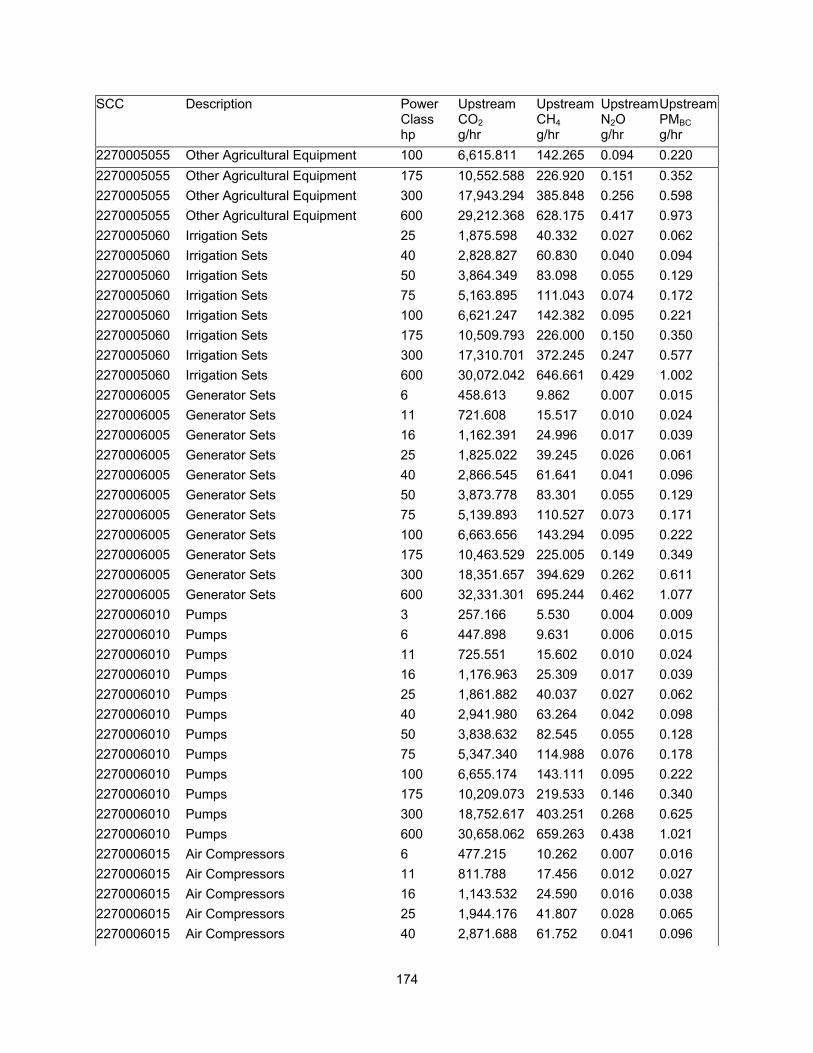
174
SCC Description Power Class
Upstream CO2
Upstream CH4
Upstream N2O
Upstream PMBC
hp g/hr g/hr g/hr g/hr 2270005055 Other Agricultural Equipment 100 6,615.811 142.265 0.094 0.220 2270005055 Other Agricultural Equipment 175 10,552.588 226.920 0.151 0.352 2270005055 Other Agricultural Equipment 300 17,943.294 385.848 0.256 0.598 2270005055 Other Agricultural Equipment 600 29,212.368 628.175 0.417 0.973 2270005060 Irrigation Sets 25 1,875.598 40.332 0.027 0.062 2270005060 Irrigation Sets 40 2,828.827 60.830 0.040 0.094 2270005060 Irrigation Sets 50 3,864.349 83.098 0.055 0.129 2270005060 Irrigation Sets 75 5,163.895 111.043 0.074 0.172 2270005060 Irrigation Sets 100 6,621.247 142.382 0.095 0.221 2270005060 Irrigation Sets 175 10,509.793 226.000 0.150 0.350 2270005060 Irrigation Sets 300 17,310.701 372.245 0.247 0.577 2270005060 Irrigation Sets 600 30,072.042 646.661 0.429 1.002 2270006005 Generator Sets 6 458.613 9.862 0.007 0.015 2270006005 Generator Sets 11 721.608 15.517 0.010 0.024 2270006005 Generator Sets 16 1,162.391 24.996 0.017 0.039 2270006005 Generator Sets 25 1,825.022 39.245 0.026 0.061 2270006005 Generator Sets 40 2,866.545 61.641 0.041 0.096 2270006005 Generator Sets 50 3,873.778 83.301 0.055 0.129 2270006005 Generator Sets 75 5,139.893 110.527 0.073 0.171 2270006005 Generator Sets 100 6,663.656 143.294 0.095 0.222 2270006005 Generator Sets 175 10,463.529 225.005 0.149 0.349 2270006005 Generator Sets 300 18,351.657 394.629 0.262 0.611 2270006005 Generator Sets 600 32,331.301 695.244 0.462 1.077 2270006010 Pumps 3 257.166 5.530 0.004 0.009 2270006010 Pumps 6 447.898 9.631 0.006 0.015 2270006010 Pumps 11 725.551 15.602 0.010 0.024 2270006010 Pumps 16 1,176.963 25.309 0.017 0.039 2270006010 Pumps 25 1,861.882 40.037 0.027 0.062 2270006010 Pumps 40 2,941.980 63.264 0.042 0.098 2270006010 Pumps 50 3,838.632 82.545 0.055 0.128 2270006010 Pumps 75 5,347.340 114.988 0.076 0.178 2270006010 Pumps 100 6,655.174 143.111 0.095 0.222 2270006010 Pumps 175 10,209.073 219.533 0.146 0.340 2270006010 Pumps 300 18,752.617 403.251 0.268 0.625 2270006010 Pumps 600 30,658.062 659.263 0.438 1.021 2270006015 Air Compressors 6 477.215 10.262 0.007 0.016 2270006015 Air Compressors 11 811.788 17.456 0.012 0.027 2270006015 Air Compressors 16 1,143.532 24.590 0.016 0.038 2270006015 Air Compressors 25 1,944.176 41.807 0.028 0.065 2270006015 Air Compressors 40 2,871.688 61.752 0.041 0.096

175
SCC Description Power Class
Upstream CO2
Upstream CH4
Upstream N2O
Upstream PMBC
hp g/hr g/hr g/hr g/hr 2270006015 Air Compressors 50 3,794.057 81.586 0.054 0.126 2270006015 Air Compressors 75 5,208.470 112.002 0.074 0.174 2270006015 Air Compressors 100 6,466.260 139.049 0.092 0.215 2270006015 Air Compressors 175 9,962.328 214.227 0.142 0.332 2270006015 Air Compressors 300 18,760.328 403.417 0.268 0.625 2270006015 Air Compressors 600 32,955.874 708.675 0.471 1.098 2270006025 Welders 11 758.040 16.301 0.011 0.025 2270006025 Welders 16 1,258.399 27.060 0.018 0.042 2270006025 Welders 25 1,825.022 39.245 0.026 0.061 2270006025 Welders 40 2,827.112 60.793 0.040 0.094 2270006025 Welders 50 3,963.786 85.236 0.057 0.132 2270006025 Welders 75 5,509.355 118.472 0.079 0.184 2270006025 Welders 100 7,697.518 165.525 0.110 0.256 2270006025 Welders 175 13,811.858 297.007 0.197 0.460 2270006025 Welders 600 34,575.138 743.495 0.494 1.152 2270006030 Pressure Washers 6 444.040 9.549 0.006 0.015 2270006030 Pressure Washers 11 775.013 16.666 0.011 0.026 2270006030 Pressure Washers 16 1,197.537 25.752 0.017 0.040 2270006030 Pressure Washers 25 1,750.444 37.641 0.025 0.058 2270006030 Pressure Washers 40 2,677.099 57.568 0.038 0.089 2270006030 Pressure Washers 50 3,884.065 83.522 0.055 0.129 2270006030 Pressure Washers 75 5,258.189 113.071 0.075 0.175 2270006030 Pressure Washers 100 6,826.354 146.792 0.097 0.227 2270006030 Pressure Washers 175 9,892.931 212.735 0.141 0.330 2270006030 Pressure Washers 300 17,441.785 375.064 0.249 0.581 2270006030 Pressure Washers 600 32,038.291 688.943 0.457 1.067 2270006030 Pressure Washers 750 53,119.564 1,142.269 0.758 1.770 2270007015 Forest Eqp - Feller/Bunch/Skidder 40 3,040.560 65.383 0.043 0.101 2270007015 Forest Eqp - Feller/Bunch/Skidder 50 3,851.491 82.821 0.055 0.128 2270007015 Forest Eqp - Feller/Bunch/Skidder 75 5,579.647 119.983 0.080 0.186 2270007015 Forest Eqp - Feller/Bunch/Skidder 100 6,928.105 148.980 0.099 0.231 2270007015 Forest Eqp - Feller/Bunch/Skidder 175 10,669.406 229.432 0.152 0.355 2270007015 Forest Eqp - Feller/Bunch/Skidder 300 17,538.324 377.140 0.250 0.584 2270007015 Forest Eqp - Feller/Bunch/Skidder 600 32,810.372 705.546 0.468 1.093 2270007015 Forest Eqp - Feller/Bunch/Skidder 750 53,681.911 1,154.362 0.767 1.789 2285002015 Railway Maintenance 11 841.585 18.097 0.012 0.028 2285002015 Railway Maintenance 16 1,429.278 30.735 0.020 0.048 2285002015 Railway Maintenance 25 1,770.160 38.065 0.025 0.059 2285002015 Railway Maintenance 40 3,372.407 72.519 0.048 0.112 2285002015 Railway Maintenance 50 4,462.826 95.967 0.064 0.149
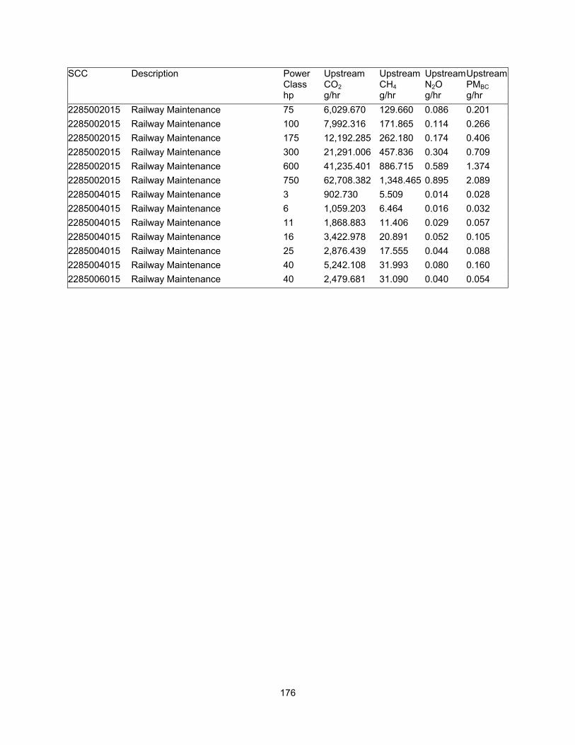
176
SCC Description Power Class
Upstream CO2
Upstream CH4
Upstream N2O
Upstream PMBC
hp g/hr g/hr g/hr g/hr 2285002015 Railway Maintenance 75 6,029.670 129.660 0.086 0.201 2285002015 Railway Maintenance 100 7,992.316 171.865 0.114 0.266 2285002015 Railway Maintenance 175 12,192.285 262.180 0.174 0.406 2285002015 Railway Maintenance 300 21,291.006 457.836 0.304 0.709 2285002015 Railway Maintenance 600 41,235.401 886.715 0.589 1.374 2285002015 Railway Maintenance 750 62,708.382 1,348.465 0.895 2.089 2285004015 Railway Maintenance 3 902.730 5.509 0.014 0.028 2285004015 Railway Maintenance 6 1,059.203 6.464 0.016 0.032 2285004015 Railway Maintenance 11 1,868.883 11.406 0.029 0.057 2285004015 Railway Maintenance 16 3,422.978 20.891 0.052 0.105 2285004015 Railway Maintenance 25 2,876.439 17.555 0.044 0.088 2285004015 Railway Maintenance 40 5,242.108 31.993 0.080 0.160 2285006015 Railway Maintenance 40 2,479.681 31.090 0.040 0.054

177
APPENDIX D. COOL PAVEMENT TECHNOLOGY
Background Information:
The US EPA describes a “heat island” as a built up area that is hotter than nearby rural areas(EPA 2010c). The impacts of the heat island effect are significant. Annual temperatures in a city of one million range from 1.8 to 5.4 deg F higher than surrounding areas (EPA 2010c). On a clear summer night the difference can be as high as 22 deg F. (EPA 2010c). This increased temperature has significant impacts on CO2 emissions in two ways. The first is through increased energy demand for cooling. Peak urban electric demand increases 1.5 to 2% for every 1 deg F increase in summertime temperature (EPA 2008b). It is estimated that 5 to 10 percent of electricity demand is used to compensate for the heat island effect (EPA 2008b). The second way is through increased formation of ground level ozone. NOx and VOCs react in the presence of sunlight to form ozone, and higher temperatures increase the rate of this reaction (EPA 2008b). One of the methods proposed by the EPA to reduce the heat island effect is the introduction of cooler pavement (EPA 2008b). The contribution of pavements to the heat island effect is often measured by the albedo of a pavement. Albedo is the surface reflectivity of the sun’s radiation (Budikova 2010). Albedo is measured in percentages with 100% Albedo meaning that all of the sun’s radiation is reflected and 0% meaning that no radiation is reflected off of a surface. As the albedo of a surface decreases, the heat island effect increases. Over 60% of US urban surfaces are either pavement or roof (Menon et al. 2010). It is estimated that a .15 increase in the albedo of 26 m2 of paved area will offset one ton of emitted CO2 (Menon et al. 2010). There are multiple new technologies available for increasing the albedo of pavements. The technologies often focus around creating a lighter colored pavement and increasing the permeability of the pavement. In an effort to increase the utilization of these new technologies the EPA has been hosting a database of local demonstration projects that include heat island mitigation measures (EPA 2010c). They can be found at: http://yosemite.epa.gov/gw/statepolicyactions.nsf/HIRIInitiative?OpenView&count=500&type=Demonstration%20Project. Asphalt Technology
One new approach to increasing albedo in asphalt is the introduction of Cool Asphalt. Traditional asphalt has an albedo of 0.04 for newly laid pavement that increases up to 0.15 as it ages (Houston Advanced Research Center (HARC) 2006). Cool Asphalt technology refers generally to asphalts that utilize white aggregates or light colors to
178
make a traditional asphalt of a lighter color. By using an aggregate that is 30-40% more reflective it is expected that the asphalt concrete could increase in reflectivity by 10 to 15% (Houston Advanced Research Center (HARC) 2006). Another approach to creating lighter asphalt involves the use of lightly colored aggregate in chip seals. Light colored chip seal increases albedo by an estimated 20% (Houston Advanced Research Center (HARC) 2006). This approach is particularly well suited to low volume asphalt roads as a resurfacing technique which will also extend pavement life (EPA 2008b). This effect can also be achieved by utilizing Ultra-thin whitetopping as a surface coating on a pavement. Whitetopping is the application of a layer of concrete over an existing asphalt surface (EPA 2008b). The albedo of a white topped asphalt surface is roughly the same as any other concrete surface (EPA 2008b). Another source of high reflectivity asphalt can come from the use of open-graded asphalt or rubberized asphalt. Open-graded asphalt is a form of asphalt that removes sand and other fine aggregates from the mixture (Houston Advanced Research Center (HARC) 2006). Rubberized asphalt is made by mixing shredded rubber into traditional asphalt (EPA 2008b). These types of asphalt allow water to permeate the pavement providing a cooling effect, reduced roadway noise, as well as improved storm water drainage (Houston Advanced Research Center (HARC) 2006). This surface type also has the added benefit of improved friction during wet weather (EPA 2008b). Other techniques to increase reflectivity in asphalt include resin based pavements which use clear tree resins as opposed to petroleum based binders (EPA 2008b). There are also colored asphalts which add pigments or seals to the asphalt mix in order to increase reflectance (EPA 2008b). Cement Technology
Cement is preferable to asphalt because it is lighter and has a higher albedo, 0.35.-04 vs. 0.05-0.1 respectively (EPA 2008b). Even as concrete ages and darkens, it retains a higher albedo than asphalt, 0.25-0.35 vs. 0.1-0.2 respectively (EPA 2008b). One of the materials that causes darkness in concrete is the presence of iron oxide in the clay substrate (Houston Advanced Research Center (HARC) 2006). White cement is a highly reflective paving material that substitutes kaolin for the ordinary clay, resulting in concrete with a much higher albedo (Houston Advanced Research Center (HARC) 2006). The use of lighter colored materials in the composition of concrete can increase the reflectance of concrete to 0.4-0.8 (Houston Advanced Research Center (HARC) 2006). Slag and Fly Ash Cement also represent a form of higher reflectivity concrete, which have additional benefits as recycled byproducts of Iron manufacturing (EPA 2008b). These products make concrete stronger, cheaper and less carbon intensive while slag

179
cement has an albedo of up to 0.6 compared with 0.35 for traditional concrete mixes (EPA 2008b). One great example of the use of slag cement is in the Detroit Airport. Local fine aggregates in the Detroit area were susceptible to alkali-silica reaction from water that infiltrated the concrete (Slag Cement Association (SCA) 2010). They used slag cement instead which reduced the permeability of the concrete, and lowered the number of alkalis in the concrete mixture (Slag Cement Association (SCA) 2010). The slag cement also produced a smoother pavement finish, increased the durability of the pavement, and produced a higher albedo surface (Slag Cement Association (SCA) 2010). Porous Pavements
Porous pavement represents another paving type that can substantially decrease the urban heat island effect. These pavements can be asphalt, concrete, or pavers; and they sometimes have lattice structures that permit grass and other vegetation to grow through them (EPA 2008b). These surfaces are generally targeted at parking lots, sidewalks, shoulders, and other areas with low traffic volume(FHWA ). These pavements reduce heat by absorbing moisture and the cooling effect of the grasses (Houston Advanced Research Center (HARC) 2006). The main benefit of these surfaces is their ability to handle ground water, and the potential to reduce the need for curbs, gutters, and storm drains (FHWA ). Many porous pavements are prefabricated and commercial examples include: GrassPave, GrassCrete, Turfstone, and StoneyCrete Pervious Pavement (Houston Advanced Research Center (HARC) 2006). Considerations
All of these technologies share similar issues which must be considered before implementing one of the new technologies. One of the biggest concerns is the determination of situations in which these techniques are suitable. The FHWA fact sheet only encourages porous pavement in areas with high soil infiltration capacity and with organizations that can perform regular maintenance (FHWA ). Testing should be done with these products to determine projects in which they may be suitable. It is also important to consider some of the many ancillary benefits of these technologies outside of heat reduction and CO2 savings. The biggest benefit is likely to be in the area of water quality and storm water runoff. Lower temperature runoff has a reduced impact on aquatic life and water ways (EPA 2008b). Permeable and porous pavements can improve the filtering of storm water and reduce the need for drains, treatment ponds, grading, inlets, and storm water pipes (EPA 2008b). Reduced pavement temperatures have also been linked to increased pavement life with a 20 deg F reduction in surface temperature lasting ten times longer (EPA 2008b). Pavements with a higher level of reflectivity also enhance night time visibility and increase safety on the roads and potentially reduce lighting costs (EPA 2008b). There is also the benefit of

180
reduced noise as permeable pavements reduce tire noise by two to eight decibels (EPA 2008b). Applications
Each cool pavement technology has a feature that may leave it unsuitable for certain applications. That can make planning for the use of these technologies difficult. The City of Chicago has done work to identify uses and design strategies for many of these cool pavement technologies. They have published a Green Alley Handbook, which provides implementation strategies, example applications, basic cost estimates, and pilot approaches for the use of these techniques in alleys and other urban settings (City of Chicago 2010).
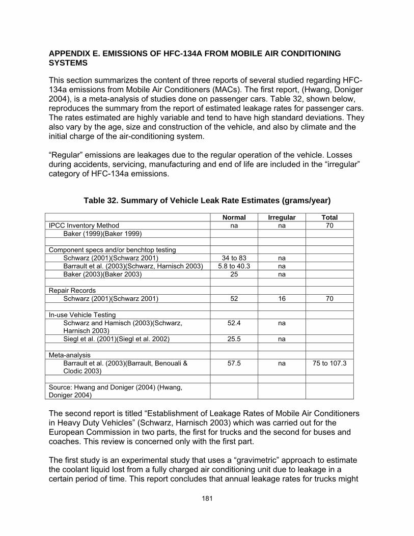
181
APPENDIX E. EMISSIONS OF HFC-134A FROM MOBILE AIR CONDITIONING SYSTEMS
This section summarizes the content of three reports of several studied regarding HFC-134a emissions from Mobile Air Conditioners (MACs). The first report, (Hwang, Doniger 2004), is a meta-analysis of studies done on passenger cars. Table 32, shown below, reproduces the summary from the report of estimated leakage rates for passenger cars. The rates estimated are highly variable and tend to have high standard deviations. They also vary by the age, size and construction of the vehicle, and also by climate and the initial charge of the air-conditioning system. “Regular” emissions are leakages due to the regular operation of the vehicle. Losses during accidents, servicing, manufacturing and end of life are included in the “irregular” category of HFC-134a emissions.
Table 32. Summary of Vehicle Leak Rate Estimates (grams/year)
Normal Irregular Total IPCC Inventory Method na na 70
Baker (1999)(Baker 1999) Component specs and/or benchtop testing
Schwarz (2001)(Schwarz 2001) 34 to 83 na Barrault et al. (2003)(Schwarz, Harnisch 2003) 5.8 to 40.3 na Baker (2003)(Baker 2003) 25 na
Repair Records
Schwarz (2001)(Schwarz 2001) 52 16 70 In-use Vehicle Testing
Schwarz and Hamisch (2003)(Schwarz, Harnisch 2003)
52.4 na
Siegl et al. (2001)(Siegl et al. 2002) 25.5 na Meta-analysis
Barrault et al. (2003)(Barrault, Benouali & Clodic 2003)
57.5 na 75 to 107.3
Source: Hwang and Doniger (2004) (Hwang, Doniger 2004)
The second report is titled “Establishment of Leakage Rates of Mobile Air Conditioners in Heavy Duty Vehicles” (Schwarz, Harnisch 2003) which was carried out for the European Commission in two parts, the first for trucks and the second for buses and coaches. This review is concerned only with the first part. The first study is an experimental study that uses a “gravimetric” approach to estimate the coolant liquid lost from a fully charged air conditioning unit due to leakage in a certain period of time. This report concludes that annual leakage rates for trucks might

182
be as high as 87.8 grams per annum, and an additional 30 g/annum might be lost due to “irregular” leakages. The third report is from a presentation to the California Air Resources Board. Titled “A Study of R134a Leaks in Heavy Duty Vehicles”(Burnette, Baker ), the study includes both trucks and off-road vehicles. It uses fleet maintenance records as well as gravimetric measurements to arrive at leakage rate estimates. The authors come up with point estimates of leakage rates.
Figure 5. Average Annualized Leak rate by Model Year Bin and Overall
(Source: Burnette and Baker 2010)
The authors find that new on-road vehicles (not older than 2006) have leakage rates of 103 g/yr and older vehicles have leakage rates of 306 g/yr. The authors make an informed assumption that all off-road vehicles have leakage rates of 306 g/yr.

183
APPENDIX F. DOCUMENTATION OF MATERIALS CALCULATIONS
General Note
Densities of all materials used in our computations are given in a separate worksheet. They are obtained from four online sources.22 Since densities are known, the computations described in this document may arrive at either the weight or the volume of materials consumed. It is to be noted that while we have estimated lifecycle emissions for basic materials such as concrete and steel, we have not been able to fully include the emissions at the last stage of manufacturing – for instance, the emissions in the manufacture of a precast concrete pipe. Direct equipment emissions due to the road project are covered in the equipment section. Densities of concrete and aggregate materials (stone/sand/coarse aggregate/soil aggregate) are only approximately determined to be 150 lb/cu.ft and 100 lb/cu.ft. Emission factors for major materials (cement, aggregate, steel and asphalt binder) are reported in a previous section of this report. For most of the other materials, the GREET vehicle cycle model is used as a source of emission factors. In the case of wood, calculations from a lifecycle analysis carried out by Puettmann and Wilson(Puettmann, Wilson 2005) are used to estimate final emission factors for carbon dioxide and methane. The authors give no estimate for nitrous oxide. A notable gap in our estimates for material emissions is our inability to obtain the emissions from brick kilns. We also do not distinguish between PVC, polypropylene and HDPE for the purposes of emission rates (g/lb). For recycled materials, the GreenDOT spreadsheet for estimating the carbon footprint of transportation construction projects is used as a source for CO2 emission factors (Gallivan 2010). We assume that other emissions (CH4 and N2O) are emitted in the same ratio as in the case of the material being replaced. (For instance, if the ratio of N2O emissions to CO2 emissions in cement production is 0.1%, then we assume that the same will hold true of any cement alternative). In the case of Ground Bituminous Shingle Material, we assume that it has the same emission factors as Recycled Asphalt Pavement (RAP). In the case of Remediated Petroleum Contaminated Soil Aggregate (RPCSA), we assume that there are no additional emissions that need to be attributed to the use of the material for construction purposes, as the remediation would have taken place regardless of its use as recycled material. Weights and dimensions of standard rebars are obtained from an online source23. Epoxy-coating, where relevant, is not estimated due to unavailability of emission data. The zinc coating in galvanized steel is estimated to weigh 3 oz per sq. ft of surface area 22http://www.simetric.co.uk/si_materials.htm http://www.coolmagnetman.com/magconda.htm
http://www.substech.com/dokuwiki/doku.php?id=thermoplastic_high_density_polyethylene_hdpe http://www.wsdot.wa.gov/research/reports/fullreports/692.1.pdf
23http://www.sizes.com/materls/rebar.htm
184
of the rebar24. The electricity consumed in galvanization of reinforcement steel has been ignored in this analysis. The same assumptions for galvanization of rebars have been used throughout this study. Rebar sizes and weights have been derived from an online source and used, often with appropriate radius adjustments.25 Subbase, Base and Surface Courses
Sections 203, 301, 302, 305– Aggregates – Cu. Yard
The volume is available directly in the input. Dense-graded aggregate (DGA) is treated to have the same emission factors as soil aggregate. Section 303, 401, 402, 403, 404– Asphalt-Aggregate mixes – Tons
Since the grade of aggregate used in asphalt-aggregate mixes is found to have negligible impacts, we treat all types of asphalt-aggregate mixes equivalently. Users have the option of changing the ratio of asphalt binder to aggregate, the amount of moisture in the mix and the temperature to which it is heated. A heating model (described previously in this report) calculates the total emissions. Section 304, 405 – Concrete Surface and Base courses – Inches x Sq. yards26
The inputs consist of the thickness and area of the concrete layer. Volume of concrete is estimated simply by multiplying area by thickness and removing the volume occupied by reinforcement steel. Users have the option of altering the ratios of cement and aggregate, which is reflected in their respective weights and by extension in the total emissions from these items. Based on detailed geometric calculations from drawings, it was determined that the volume of steel used in concrete courses is 0.001392 cu. ft. per sq. ft for surface courses and reinforced base courses less than ten inches thick and 0.002013 cu. ft. per sq. ft for concrete surface and reinforced base courses ten inches thick or more. This is based on a twenty foot lane width. We assume that all concrete surface courses are reinforced. Section 401 – Asphalt Binder – Type – Gallons
Tack and Prime Coats consist primarily of heated binder material, and are treated as such. Calculations for cut-back asphalt also consider emissions from vaporization during the heating process.
24http://www.galvanizeit.org/aga/inspection-course/galvanizing-standards/astm-a-767-a-767m 25 http://www.sizes.com/materls/rebar.htm 26 STANDARD ROADWAY DETAILS (English units) 2001; CD-405-1, SHEET 14
185
Section 203, 401, 603 – Geotextiles and Reinforcement Meshes – Sq. Yard
Geotextiles are estimated to weigh 0.25 lb/sq.yard based on Maine Government specifications27. Geotextile plastics are assumed to have similar emission factors as polypropylene. Another source suggests approximately 3 lb/ sq. yard as the density of a steel reinforcement mesh (which is also used to estimate the density of Pavetrac).28 Bridges and Structures
Section 501 – Temporary/Permanent Sheeting – Sq. Yard
All sheeting is assumed to be made of stamped steel, which, based on a manufacturer’s specification, is estimated at 31.7465 lb/sq.ft.29 For cofferdams,another manufacturer’s drawings are used to estimate that 1.78 cu. Ft. of aluminum will be used to produce one unit of this product.30 Section 502 – Cast-in-place piles – Feet
We assume that cast-in-place piles are akin to filled cylinders with the given nominal diameter. The casing is assumed to have the same geometry as a seamless steel pipe pile of the given diameter, except in the case of 30” and 36” piles, where a 0.3 inch thick pipe is assumed. The weights of seamless steel pipe piles are obtained from Fuller (1983)(Fuller 1983). Reinforcement is assumed to consist of 12 #5 axial bars and spiral bars at 6 inch intervals. The spiral bars are 2.5 inch from the concrete surface. Section 502 – Precast and pre-stressed concrete piles – Feet
Precast and Prestressed concrete piles are estimated with perfect square cross-sections. Reinforcement is assumed to consist of 12 #5 axial bars and spiral bars at 6 inch intervals. The spiral bars are 2.5 inch from the concrete surface. Section 502 – Steel H-piles and timber piles – Feet
Cross-sectional areas (in sq. inch) of Steel H-Piles are obtained from Fuller (1983) (Fuller 1983). Timber piles are estimated to be perfect cylinders of 12” diameter. Steel Soldier Piles are assumed to have the same material content as 12” x 74” Steel H-piles.
27http://www.maine.gov/mdot/mlrc/geotextiles.php 28 http://www.acfenvironmental.com/PDFs/PavPreservation/Install%20-%20with%20Slurry%20Seal%20-%2010-10-03.pdf (p. 4) 29http://www.skylinesteel.com/assets/ProductBrochures/GenProductBrochUS.pdf 30http://www.supsalv.org/pdf/7370421g3.pdf
186
Section 504 – Reinforcement Steel - Tons
Users are required to input reinforcement steel in tons. To enable an estimation of the quantity of zinc, the reinforcement bars are assumed to be of the #10 size. Section 504 – Structural Concrete –Cu. Yard
Given the volume, the estimate for density of concrete is used to estimate total emissions. HPC, HES and VESLMC concrete are all assumed to be equivalent to traditional concrete mixes (users do have the option of altering the cement/aggregate ratios). Section 505 – Pre-tensioned Pre-stressed concrete beam – Inches x Feet
The concrete content had to be estimated volumetrically, using the NJDOT drawings for the four sizes of Pre-tensioned, Pre-stressed beams.31 Similarly, the length and size of each reinforcement bar was accounted for, as was the zinc contained in those rebars which were specifically required by NJDOT to be galvanized. The steel in the hooks inserted at the end of each beam at the time of casting was not included for the sake of simplicity. For estimation purposes, we considered beams of 54’ to be typical. For the beam of height 93.5 inches, the drawing of the 72” beam was adopted – essentially by assuming that while the height of the beam changed, it only lengthened the neck of the beam and didn’t affect the cross-section otherwise. Section 505 –Pre-stressed concrete box-beams and slab-beams – Inches x Inches x Feet
Texas DOT drawings of box-beams and slab-beams were used to estimate the quantity of concrete, steel and zinc in them.32 However, to the extent that there was an incongruity in the sizes of beams used in the two states, the drawings often had to be modified to fit the dimensions included in the NJDOT bid-sheets. Section 505 – Channel beams – Inches x Inches x Feet
A product drawing from a manufacturer served as a reference in the estimation.33 Section 505, 602 – Precast Concrete Culverts – Feet/Cu. Yards
An NJDOT drawing was used as a reference for concrete culverts.34 We assume a 4’ x 4’ culvert with a maximum depth of fill of 15 ft, for which NJDOT provides the volume of
31NJDOT Bridge Manual Standard Drawing Plates- Sheet SP 2.4-1 NJDOT Bridge Manual Standard Drawing Plates- Sheet SP 2.4-2 NJDOT Bridge Manual Standard Drawing Plates- Sheet SP 2.4-3 NJDOT Bridge Manual Standard Drawing Plates- Sheet SP 2.4-4 32Texas DOT Bridge Standards (English) – BB-B34 Texas DOT Bridge Standards (English) – PSB-4SB15 33http://www.mccannconcreteproducts.com/images/Channel%20Beam%20Superstructure.pdf

187
concrete and weight of reinforcement steel needed per foot. In Section 505, the input is in Feet, and the values obtained are used directly. In Section 602, the input is in cubic yards. We estimate concrete simply by the volume inputted. For reinforcement steel, the volume of concrete is reduced to a length based on an assumed average cross-sectional area of 8 sq. ft, and the resulting length is then used to estimate the weight of reinforcement steel used. Section 602 –Concrete Headwall – Cu. Yard
We assume square headwalls. The volume input (reduced, the volume of steel) is taken to be the volume of concrete used. A FHWA drawing suggests the appropriate amount of reinforcement steel for a given volume of concrete.35 When this relationship is modeled as a linear relationship, the regression has an R2 of 0.99, and the coefficient is 85.39 lb of reinforcement steel per cu. Yd. of concrete. This rate is used to estimate the amount of steel needed. Section 505 – Precast Concrete Arch structures – Feet
A product brochure is used to obtain recommended weight for bridge arch structures, assuming a 12 feet rise and a 48 feet span.36 The weight of concrete needed is 5.67 ton per feet of arch structure. As no information about the steel requirements is available, we assume a steel/concrete ratio of 85.39 lb/cu.yard which is also obtained for concrete headwalls. Section 505 – Superstructures and Deck panels – Sq. Feet
We assume that the material requirements are akin to the requirements of a concrete slab of the given area and 2’ thickness. A steel/concrete ratio of 80 lb/cu.yard is assumed. Section 506 – Structural Steel – Tons/Pounds (Direct)
Section 507 – Bridge Decks and approach slabs; median, moment and bridge-relief slabs – Cu. Yard
For all concrete bridge decks and approaches, the amount of concrete is obtained directly from the input (less, the volume of concrete). Based on a drawing from Texas DOT, reinforcement steel is estimated for 13” thick decks and reinforcement at 8.5lb/sq. foot37. Assuming the reinforcement bars to be of #5 size allows the amount of zinc to be estimated. Median, moment and bridge-relief slabs are assumed to have the same geometry as approach slabs. All types of concrete are treated to be equivalent.
34NJDOT Roadway construction Details (English Units) 2001; CD-610-2 (SHEET NO. 41) 35Federal Lands Highway Standard Drawing 601-1 for Concrete Headwalls, accessed at http://flh.fhwa.dot.gov/resources/pse/standard/st60101.pdf 36http://www.contech-cpi.com/Products/Bridges-and-Structures/Precast/CONSPAN-Bridge.aspx 37Texas DOT Bridge Standards (English) – BAS-C

188
Section 507 – Bridge Sidewalks – Cu. Yard
The amount of concrete is obtained directly, as in the case of approach slabs. Reinforcement concrete is estimated using the same estimate as concrete surface courses, i.e. 0.0089 cu. ft per sq. foot of sidewalk. Section 507 – Bridge Parapets – Feet
Concrete parapets are assumed to be of the type of 2’ 10” height. An NJDOT drawing for these types of parapets is used to estimate the volume of concrete to be 3.68 cu. Ft of concrete per feet of parapet.38 Reinforcement steel is estimated at 255.05 lb per foot of parapet. All types of concrete are dealt with equivalently. Open steel parapets are estimated at 0.268 cu. Ft of stamped steel per foot of parapet, based on a similar NJDOT drawing.39 Half Concrete Barriers are assumed to have similar geometries as bridge parapets. Section 507, 607 –24” and 15” Concrete Barrier Curbs – Inches x Inches x Feet
Estimations for Concrete barrier curbs of various heights are carried out using the drawings made available by NJDOT.40 Concrete is estimated volumetrically, while reinforcement steel requirements are measured in lb/ft. When not specified, barrier curbs are assumed to be of the 24” x 32” size. Dowelled curbs are treated to be the same as common barrier curbs. Section 507 – Median barriers – Inches x Inches x Feet
Median barriers in Section 507 are assumed to have the same outside geometry as 24” x 32” barrier curbs while having a greater quantity of reinforcement steel, as shown in an NJDOT drawing.41 Section 507, 607 – Concrete Vertical and Sloping Curbs – Inches x Inches x Feet
Estimations for Concrete vertical and sloping curbs of various heights are carried out using the drawings made available by NJDOT.42 Where dimensions are missing, a size of 9” x 6” is assumed. Dowelled curbs are assumed to have the same materials requirements as usual vertical curbs. White concrete is estimated in the same manner as normal concrete.
38NJDOT Bridge Manual Standard Drawing Plates- Sheet BCD-507-2 39NJDOT Bridge Manual Standard Drawing Plates- Sheet BCD-507-10 40NJDOT Roadway construction Details (English Units) 2001; CD-605-3 (SHEET NO. 36) 41 NJDOT Bridge Manual Standard Drawing Plates- Sheet BCD-507-9 42NJDOT Roadway construction Details (English Units) 2001; CD-605-1 (SHEET NO. 34) NJDOT Roadway construction Details (English Units) 2001; CD-605-2 (SHEET NO. 35)

189
Section 607 – Variable height/width Barrier/Vertical Curbs – Inches x Feet
Estimations are made based on the closest “standard” prototype of curbs whose height/width is known. For instance, for barrier curbs, a height of 32” is considered “standard”, and for vertical curbs, a size of 6” is assumed to be the “standard”. Section 607 – Granite/Belgian Block/Bluestone Curbs – Feet These curbs are assumed to have the same geometry as 9” x 6” vertical curbs and the same emission factors as aggregates. Emissions from cutting the granite are not included at this stage (they might be included in the equipment stage). Section 607 – HMA Curbs – Inches x Inches x Feet
Estimations are made based on the assumption that the curbs have the same geometry as the corresponding concrete curbs. The volumes are converted to tons of HMA using an estimate of the density of HMA. Section 509, 605 – Bridge Railing/Handrails – Feet
Based on a volumetric approach, the volume of metal required to manufacture rails, post bases, stems and splices is estimated from NJDOT drawings.43 The metal might be either steel or aluminum based on the item specifications. Handrails and rail & post fences are assumed to have the same geometry as bridge railing. Ornamental Railing is also assumed to have the same geometry as bridge railing. Section 509, 605 – Chain-link fences – Feet x Feet (or units x feet)
An NJDOT drawing provides the relative dimensions of the various posts and rails used to hold the fence, given its height and length.44Using a product manufacturer’s specifications, the weight of the fabric per foot of fence is obtained as a function of the height.45 The fabric is assumed to be of 9 gauge and 2” mesh. Specifications for line posts and top rails are obtained from Ohio DOT46. These specifications make it possible to estimate the weight of these elements per foot of fence. Aluminum-coating, where specified, is estimated at 0.4 oz/sq.ft.47 Similarly, the weight of zinc is estimated for galvanized fences using previously used assumptions regarding galvanization.48 In the case of PVC-coated chain-link fences, the contributions of the PVC to total emissions are not included. In this case, it is assumed that the rails and posts are galvanized.
43NJDOT Bridge Manual Standard Drawing Plates Sheet 509-3 NJDOT Bridge Manual Standard Drawing Plates- Sheet 509-4 44NJDOT Roadway construction Details (English Units) 2001; CD-614-1 (SHEET NO. 59) 45http://www.buildersfence.com/ChainLink_Pages/ChainLFabric-Blank.pdf 46http://www.dot.state.oh.us/Divisions/ConstructionMgt/Materials/TAS%20Manual/TAS-Manual-Tranning/ChainLinkFence.pdf 47http://www.soncoww.com/customer/astm.asp 48http://www.galvanizeit.org/aga/inspection-course/galvanizing-standards/astm-a-767-a-767m

190
Goose exclusion fences, ornamental and rock-catch fences, and several other items are assumed to have the same geometry as chain-link fences. Fence gates were all assumed to be 6’ high, and their width is to be inputted. Section 512 –Overhead Sign support structures – Units
Assuming a structure of span 95 feet, height 30 feet, width 4 feet and depth 5 feet, we arrive at estimates of sheet metal in the truss structures, concrete in the foundation and rolled steel for reinforcement. An NJDOT drawing is used for the dimensions.49 Bridge-mounted support structures are assumed to have the same geometry. Section 512 – Cantilever/Butterfly Sign support structures – Units
Assuming a structure of span 40 feet, height 30 feet and depth 5 feet, we arrive at estimates of sheet metal in the truss structures, concrete in the foundation and rolled steel for reinforcement. An NJDOT drawing is used for the dimensions.50 Butterfly structures share the same types of cantilevers, but use twice the amount of metal for truss elements. Section 512 – Steel post support – Units
Based on an NJDOT drawing, the weight of a 12’ long support is determined to be 30 lb. Monotube supports are assumed to have the same weight.51 Section 512, 612 –Signs – Sq. Foot
Based on NJDOT specifications, the thickness of the aluminum plate is taken to be 0.1 inches52. Where the item specified includes the supports, it is assumed that signs are of size 30” x 30”. The number of signs thus calculated, is multiplied by 30 lbs to obtain the weights of the supports. Miscellaneous Items and Utilities
Section 601 –Corrugated Aluminum Pipes – Inches x Feet
Given the diameter and the length of the pipe, the nominal thickness of the pipe is used to estimate volume. Pipe bedding and embankments are not included in this estimate. From NJDOT specifications, it is determined that thickness for aluminum pipes must be at least 0.06 inches.53 The use of nominal diameter assumes that the perimeter of a corrugated pipe would be the same as that of a smooth pipe.
49NJDOT Bridge Manual Standard Drawing Plates for Overhead Sign Support Structures (OH-G4) 50NJDOT Bridge Manual Standard Drawing Plates for Cantilever Sign Support Structures (CA-G3) NJDOT Roadway construction Details (English Units) 2001; CD-619-5 (SHEET NO. 78) 52http://www.state.nj.us/transportation/eng/specs/2007/spec900.shtm#s911 53http://www.state.nj.us/transportation/eng/specs/2007/spec900.shtm#s9090204
191
Section 601 – Corrugated Steel/Metal Pipes – Inches x Feet
Given the diameter and the length of the pipe, the nominal thickness of the pipe is used to estimate volume. From NJDOT specifications, it is determined that thickness for steel pipes must be at least 0.079 inches.54 Corrugated metal pipes are assumed to be made of steel. The use of nominal diameter assumes that the perimeter of a corrugated pipe would be the same as that of a smooth pipe. Section 601 – Reinforced Concrete Pipes, Cured-in-place pipes – Inches x Feet
The weight of concrete to be used in manufacture of reinforced concrete pipes is obtained from the Concrete Pipe Design Manual published by the American Concrete Pipe Association.55 Reinforcement is assumed to consist of 12 #5 rebars axially, and a spiral # 5 rebar for cross-sectional reinforcement which completes a circle at 6” intervals. The diameter of the spiral rebar is assumed to be the same as the nominal diameter of the pipe. It is assumed that the class of concrete does not impact the emission factors. Cured-in-place pipes maintain the same geometry, but have slightly different emission factors. Section 601, 651, 652 – HDPE Pipes, PVC pipes, outlet drains, underdrains – Inches x Feet
For HDPE (high density polyethylene) and PVC (Polyvinyl chloride) pipes, we use emission factors for polypropylene as an approximation, since GREET does not report emissions for HDPE or PVC. Weights of various sizes of HDPE pipes are obtained from a manufacturer’s brochure.56 Underdrains are assumed to be identical to 6” HDPE pipes, and all other parts of underdrains are ignored in this estimation.57 PVC pipes in Sections 601 and 651 have weights as specified in an online engineering source58and the weights of PVC sewer pipes in Section 652 is found in a product brochure and used with appropriate radius adjustment where necessary.59 The radius adjustment accounts only for the increase in the diameter and not the increase in thickness of the pipe. Section 601, 652 – Corrugated Aluminum/Steel/Metal Pipe Arch – Inches x Inches x Feet
We continue to use 0.06 inches thickness for aluminum pipes and 0.079 inches thickness for steel/metal pipes.60 The perimeter of the pipe is approximated using Ramanujan’s first approximation for an ellipse (Ramanujan 1914).
54http://www.state.nj.us/transportation/eng/specs/2007/spec900.shtm#s9090204 55 Concrete Pipe Design Manual by American Concrete Pipe Association, 3rd Edition 1970, p. 67 56http://www.ads-pipe.com/pdf/en/Product_Note_3.108_N-12_Specification_for_Leachate.pdf 57http://www.state.nj.us/transportation/eng/CADD/v8/v8RoadwayDetails/pdf/034_CD-601-1Underdrains.pdf 58http://www.engineeringtoolbox.com/pvc-cpvc-pipes-dimensions-d_795.html 59http://www.pwpipe.com/literature/w/ucshort.pdf 60http://www.state.nj.us/transportation/eng/specs/2007/spec900.shtm#s9090204

192
Perimeter ~ 3 3 3 Where ‘a’ and ‘b’ are taken as half of the rise and span of the pipe arch. Section 601 – Elliptical Reinforced Concrete Pipe – Inches x Inches x Feet
The weight of concrete to be used in manufacture of reinforced concrete pipes is obtained from the Concrete Pipe Design Manual published by the American Concrete Pipe Association(American Concrete Pipe Association 1970) (p.68). Reinforcement is assumed to consist of 12 #5 rebars axially, and a spiral # 5 rebar for cross-sectional reinforcement at 6” intervals. The estimation of the amount of steel is based on the “effective diameter” of the pipe as give in the above source. It is assumed that the class of concrete does not impact the emission factors. Section 601, 651, 652 – Ductile Pipe – Inches x Feet
We use a volumetric method similar to that used for aluminum steel pipes. A product brochure specifies the appropriate thicknesses for ductile iron pipes of the 350 pressure class as a function of the diameter.61 The same method is also used to estimate the amount of ductile iron in ductile iron water pipes (Section 651) and ductile iron sewer pipes (Section 652). We assume that ductile iron has the same emission factors as cast iron. The reinforcement is assumed to be 12 axial #5 rebars and one #5 spiral rebar at 6” intervals. At small sizes, this assumption possibly presumes an unrealistically high quantity of steel – however we continue to use this assumption for the sake of consistency. Section 601 –Pipe end sections – Inches x Feet
Pipe end sections are estimated by making the unrealistic assumption that they maintain the same cross-section as a pipe of their diameter, and have a length as specified in the pipe end section drawings.62 Section 602 – Inlets – Number x Feet
The materials requirements of Inlets of various types are estimated based on the NJDOT drawings for inlets.63 NJDOT requires the weight of the cast iron inlet cover (typically a bicycle-friendly grate) to be at least 325 lb. Similarly, the weights of the frame, the back and the curb are given in the drawings. Concrete requirements are estimated based on NJDOT requirements regarding the thickness of walls and the foundation.64 Stage 2 of the foundation (the invert) is not included in the estimate. The
61http://www.uspipe.com/Files/20047231412260.001DuctileIronPD.pdf, Table 2 62http://www.state.nj.us/transportation/eng/CADD/v8/v8RoadwayDetails/pdf/035_CD-601-2PipeEndSections.pdf 63NJDOT Roadway construction Details (English Units) 2001; CD-603-2 (SHEET NO. 25) NJDOT Roadway construction Details (English Units) 2001; CD-603-3 (SHEET NO. 26) NJDOT Roadway construction Details (English Units) 2001; CD-603-4 (SHEET NO. 27) NJDOT Roadway construction Details (English Units) 2001; CD-603-5 (SHEET NO. 28) 64NJDOT Roadway construction Details (English Units) 2001; CD-603-1 (SHEET NO. 24)

193
depth of the inlet is accepted as an input, with a default value of 12 feet. Reinforcement for the concrete consists of #13 bars at 18” centre-to-centre for vertical rebars and a varying frequency for horizontal rebars.65 We assume that most inlets have similar geometries as the 8 inlet types listed in the left-hand column of the Table XXX given below. The table describes the base drawing, and lists the inlet types which are assumed to be equivalent to the given inlet types.
Table 33. Inlet geometry
Type Other Types assumed to be similar Dimensions Casting Weight (lb)
A A – Modified, Double A, 48 x 22 565 B C, B- modified, Y, Double B, Double B modified, Special Type B, Type C
infiltration, Drain inlet, B-W, BY, BY modified, Non-standard, 48 x 42 924
E Es, Double E, 48 x 42 1085 B-1 B-1 modified, Double B-1 modified, Double B1, B1R, B1R Modified, BX,
CX 48 x 54 924
B-2 D-2, B-2 modified, Double B-2, B2R, B3R, B2X, B-4, D-3, D-4, B2Y, D2Y2, B3, Double B2R,
48 x 66 924
D-1 D modified, D, 48 x 30 924 E-1 E1X, E1Y, S, EX 48 x 54 1085 E-2 E2, E5, E3W, E3X, E4, E4W, E5W, 48 x 66 1085 Section 602, 652 – Manholes – Number x Feet
The materials requirements of Inlets of various types are estimated based on the NJDOT drawings for inlets.66 NJDOT requires the weight of the cast iron manhole cover and frame together to be at least 1030 lb. For the sake of simplicity, we assume all manholes to be made of concrete (manholes are sometimes made of brick) and perfectly cylindrical in shape (though part of the cross-section is conical). Only the first stage of the foundation is included in this estimate. For steel reinforcement, we use the same standards as used in the case of inlets.67For manholes of section 652, we assumed a height of 12’. Section 603 –Concrete Slope Gutter/Slope Protection, Shotcrete – Sq. Yard x Inches
Concrete volume is estimated simply as the product of area and thickness. In the case of reinforced slope protection, the reinforcement steel estimate for concrete surface courses is used, i.e. 0.0089 cu. ft. per foot. Shotcrete is assumed to be similar to precast concrete in composition. 65NJDOT Roadway construction Details (English Units) 2001; CD-603-1 (SHEET NO. 24) 66NJDOT Roadway construction Details (English Units) 2001; CD-603-8 (SHEET NO. 31) NJDOT Roadway construction Details (English Units) 2001; CD-603-9 (SHEET NO. 32) 67NJDOT Roadway construction Details (English Units) 2001; CD-603-1 (SHEET NO. 24)

194
Section 603 – Riprap Stone Slope/Channel Protection – Sq. Yard x Inches
The amount of aggregate (riprap) is estimated simply as the product of area and thickness. The coarse aggregate subbase layer and any possible geotextile requirements are not included. The emissions of cutting and laying granite (Granite Slope Protection) are also assumed to be the same as any aggregate. Emissions due to granite cutters may be included in the equipment stage. Section 603 – Rock Backfill/Riprap Stone Scour Protection – Tons/ Cu. Yard– Direct
Section 603 – (Articulated) Concrete Block Matting – Sq. Yard x Inches
Specifications are obtained from a product manufacturer’s brochure.68 It is assumed as a default that open-cell matting is used. 6” blocks are estimated to weigh 49 lb per sq.ft, 4.75” blocks are estimated at 40 lb per sq. ft and 8.5” blocks are estimated to weigh 70 lb per sq. ft. For 6” block closed-cell matting, we estimate a weight of 59 lb per sq. ft. These estimates are based on the averages of the given ranges and in the case of 8.5” blocks, assume on a proportional increase in the weight of 6” blocks. Section 604 – Gabion Wall/Mattress/Channel Lining – Cu. Yard
The volume of concrete is used directly. Any possible reinforcement steel requirements are not taken into account. Section 606 – HMA Sidewalks/Driveways/Islands – Sq. Yard x Inches
The volume is estimated as the product of area and thickness, and converted into tons of HMA by multiplying with the density of a typical asphalt-aggregate mixture. Section 606 – Concrete Sidewalks/Driveways/Islands, Concrete Pavers – Sq. Yard x Inches
The volume is estimated as the product of area and thickness. No reinforcement steel is included in this estimate. Tinted/Colored/White/Raised concrete sidewalks or islands are treated equivalent to the normal concrete surfaces. Section 606 – Concrete Sidewalks/Driveways/Islands – Sq. Yard x Inches
The volume is estimated as the product of area and thickness. Reinforcement is assumed to be the same as for concrete surface courses.
68http://www.shoretec.com/shoreloc.php

195
Section 606 – Brick/Granite Pavers – Sq. Yard x Inches
The volume is estimated as the product of area and thickness. Both brick and granite are assumed to have the same emissions as plain aggregate. The emissions from brick kilns and granite cutting are ignored for the purpose of this estimation. Emissions from granite cutting might be included in the equipment stage. Section 608 – Non-vegetative surface, HMA/Broken Stone – Sq. Yard x Inches
The volume is estimated as the product of area and thickness and then converted to tons of HMA using a density estimate of asphalt-aggregate mixtures. Porous, permeable, and color-coated asphalt are assumed to have the same emission factors as the usual asphalt-aggregate mixtures. Where the surface is made of stone, the volume is calculated assuming 3” thickness and converted to pounds of aggregate. Section 608 – Non-vegetative surface, Polyester Matting – Sq. Yard
Polyester matting is assumed to have similar emission factors as a geotextile fabric and treated as such using the density of geotextiles as a reference.69 Section 609 –Beam Guide Rails – Feet
Rail elements and posts, which may also be listed as separate item numbers are calculated separately. We use an NJDOT drawing to estimate the volume of stamped steel used in beam guide rail.70 We use separate galvanization factors for the additional weight of zinc on galvanized steel.71 Wood in the spacer is also estimated volumetrically. Bridge and powder-coated beam guide rails are assumed to have the same emission factors. Section 609 –Beam Guide Rails, Dual-faced – Feet
We use the same NJDOT drawing as for simple beam guide rails in this estimation too.72 The only difference is that there is a requirement for twice as much of rail element. Section 609 –Modified Thrie Beam Guide Rails (Single/Dual-faced) – Feet
Modified thrie beam guide rails have a different rail profile whose volume per feet is calculated using similar procedures as in the case of traditional beam guide rails.73 Dual-faced thrie beam guide rails have twice as much of rail element.
69http://www.maine.gov/mdot/mlrc/geotextiles.php 70NJDOT Roadway construction Details (English Units) 2001; CD-612-1 (SHEET NO. 43) 71http://www.galvanizeit.org/aga/about-hot-dip-galvanizing/what-is-hot-dip-galvanizing/the-hdg-coating/zinc-coating/#inline 72NJDOT Roadway construction Details (English Units) 2001; CD-612-2 (SHEET NO. 44) 73NJDOT Roadway construction Details (English Units) 2001; CD-612-12 (SHEET NO. 54)

196
Section 609– Rub Rail – Feet
The material volumes are estimated using an NJDOT diagram.74 Powder-coated rub-rail is assumed to have the same emission factors as rub rail. Section 609– Beam guide rail anchorages, block-outs and terminals – Units
The material volumes are estimated using an NJDOT diagram.75For anchorages, we include only the rail element and not the cables or the foundation. All guide rail terminals (irrespective of their type) are assumed to consist of one beam guide rail anchorage and 41 ft of beam guide rail element. The stamped steel requirement for block-outs was obtained from a drawing of the NYSDOT.76 Guide rail posts are assumed to be of the same dimensions, irrespective of the dimensions specified in the item. Section 653– Gas Mains – Feet
The thickness of the mains is calculated using a “thickness calculator” prepared by a manufacturer of Gas Mains.77 Gas Mains are assumed to be made exclusively of steel.
74NJDOT Roadway construction Details (English Units) 2001; CD-612-3 (SHEET NO. 45) 75NJDOT Roadway construction Details (English Units) 2001; CD-612-5 (SHEET NO. 47) 76https://www.nysdot.gov/main/business-center/engineering/cadd-info/bridge-details-sheets-repostitory-usc/BD-RC4E.pdf 77 http://www.advancepipeliner.com/Resources/Calculators/ASMEWallThickness%201.01.php

197
APPENDIX G. DATA AND ASSUMPTIONS FOR RAIL CAPITAL PROJECTS78
This section describes the process and assumptions made in estimating lifecycle greenhouse emissions for components of a rail system including track, catenary systems, tunnels, bridges, stations, parking facilities, and rolling stock. We first make an inventory of material and energy inputs of these components identifying the materials and quantifying them by weight and by volume in the case of timber ties. The next step is to identify valid emission factors by unit weight or volume. The component emission factors are summarized as the product of weight or volume per unit, and emission factors by weight or volume. These emission factors include upstream and direct emissions for carbon dioxide (CO2), methane (CH4), and nitrous oxide (N2O). Our assumptions do not include all components of downstream emissions from materials disposal and recycling. Material inputs were taken from a variety of sources including American Railway Engineering and Maintenance-of-Way Association AREMA literature and vendors’ specifications for track. A European source (Network Rail ) estimates catenary wire systems, tunnels, bridges, and rolling stock. Their estimation for passenger stations is not usable because it is on a per unit distance basis that is not generalizable to the United States. In addition, the estimate for energy use for passenger stations is based only on concrete and brick. However, they present reasonably valid and usable approximations for copper, wood, and brick, by weight. A doctoral dissertation Life-cycle Environmental Inventory of Passenger Transportation in the United States (Chester 2008) was consulted to address various gaps. From this monograph we extract light rail assumptions for track, and average specifications for heavy rail, commuter rail and light rail stations, and specifications for parking facilities including parking lots and parking garages. The rail portion of Chester is based on five rail systems including the Bay Area Rapid Transit system (BART), the Caltrain commuter line, The San Francisco Municipal Transportation Authority’s Muni line, the Boston Green Line, and the design specifications for the California High Speed Rail (CAHSR) system. Material emissions factors were taken from a variety of sources with somewhat divergent methodologies. Our method for accounting for greenhouse gas (GHG) emissions from material inputs to capital projects is to establish the energy consumption and fugitive emissions of those materials usually by weight, although it is also possible to do this by volume. This is done for every stage of the life of the material including extraction, transportation, refining and manufacturing, delivery, use or consumption, and disposal. GHG emissions from the use or disposal stage is referred to as direct emissions while everything before or after that stage is referred to as indirect emissions (Climate Registry 2008, Greenhalgh et al. 2005, Raganathan et al. 2009). Indirect emissions include upstream emissions, i.e. those emissions prior to consumption and downstream emissions, i.e. those associated with disposal or recycling. Electricity from the grid is generally considered indirect emissions because its production is outside of the consumer’s control, hence consumers are not directly responsible for the emissions.
78 The work for this portion of the project was partially funded by TCRP H41, “Assessing and Comparing Environmental Performance of Major Transit Investments”.

198
Substantial effort was made to support high per unit weight emission factors for the copper used primarily for overhead catenary wire. It is estimated that for electrified rail systems 138 metric tons of copper are present for every route-kilometer (Network Rail ). The steel in rails, the rail bed, and overhead structures and wires is estimated at 821 metric tons. The copper included in the combined rail and catenary systems amounts to 16.8% of the steel by weight. This is a substantial fraction of the total materials used in an electrical rail system, and thus must be accounted for in an emissions analysis. The Components of Track
As described in AREMA’s Practical Guide to Railway Engineering (Riley 2003), track consists of two parallel steel rails that sit on a supporting system that must restrict their movement under the heavy loads of trains of different types. Two rails are kept at a fixed distance from each other by ties that may either be precast pre-stressed reinforced concrete or pressure treated lumber. Concrete and timber ties are connected to rail with different hardware, which is addressed below. Rail segments are spliced with two steel joint bars that are bolted on either side of rail ends. Continuous rolling has increased maximum rail lengths to 1,600 feet, roughly 20 to 40 times what was possible previously. As a result the use of joint bars is diminished but not eliminated. Ballast on top of a stable base and subbase provide a medium for stabilizing track in relation to the ground. Rail anchors are attached to ties and held in place by ballast in areas subject to longitudinal motion because of changing temperature, grade, and because of traffic patterns or unusually high frequency of brake applications (Riley 2003). This section presents the material inputs of the components of commonly used track sizes and a volumetric or weight-based assessment of the material inputs of a mile of track of 100 pounds per yard. We have gathered data for track of a variety of sizes but since the Denver case and the rail systems covered in Chester (Chester 2008) are based on 100 pound track it is convenient to use this size for illustrative purposes in this methodology. Rail
Track is steel rolled in an inverse “T” shape with a massive rounded area on the end of the stem (Riley 2003). The bar of the inverted T shape provides stability while the more massive stem accommodates steel wheels of locomotives and rolling stock. A thinner section between the base and the running surface is called the web. Rail size is determined by its mass stated in terms of pounds per yard (lbs/yd) in the United States. Medium tonnage track is suitable for non-light rail transit purposes (Riley 2003). This track usually has a 5.5 inch base section and is rated 115 or 119 lbs/yd. Heavy tonnage track usually has a 6 inch base section and is rated 132, 133, 136, 140 and 141 lbs/yd. Actual weights per yard differ slightly from the nominal designations (AREMA 2000b). Light tonnage track, used for many light rail transit purposes are usually either 90 or 100 lbs/yd. Other rail sizes are discussed in the literature (Riley 2003) but will not be incorporated because their use is either rare or they are obsolete. New rail comes in 39
199
foot or 80 foot lengths, which may be welded together in lengths up to 1,600 ft (0.30303 miles). To estimate the GHG emissions from rail alone, this model uses the assumptions from the Greenhouse Gases, Regulated Emissions, and Energy Use in Transportation (GREET) model (Argonne National Laboratory 2009) for rolled steel GHG emissions grams per ton and the calculated mass of the rail in tons using the following formula to determine mass:
QtySteelrail = Size * 2 * 1760 / 2000 Where QtySteelrail is the mass of steel in the rail; Size is the track size in lbs/yd; 2 is the number of tracks; 1760 is the number of yards per mile; and 2000 is the number of pounds per ton. For example a mile of 100 lbs/yd track would weigh 100 * 2 * 1760 /2000 = 176 tons from the steel in the rails alone. Ties
Track ties are made of pressure treated timber, pre-stressed precast concrete, steel, or alternative materials (Riley 2003). Ties made of steel and alternative materials are not in wide use and will not be included in this model. Based on Chester (Chester 2008) regional lines are assumed to use concrete ties as specified above and light-rail transit lines are assumed to use timber ties. BART, Caltrain, and CAHSR are heavy, commuter, and inter-city rail respectively, and use concrete ties with a volume of six cubic feet and are spaced every 24 inches from center to center. The Muni line and the Boston Green Line are both light-rail systems and use timber ties.79 Timber Ties
Timber ties may be hardwood or softwood. Softwood ties are more resistant to rot but are less sturdy than hardwood ties and are preferred for bridges over hardwood ties. Hardwood ties are preferred for most other types of track. Hardwood ties represent 92% of timber ties while softwood ties represent 8% (Smith, Bolin 2010). Commonly used timber tie sizes are 7 * 9 * 102 inches and 7 * 9 * 108 inches or 3.719 cubic feet and 3.938 cubic feet, respectively (Riley 2003). Concrete Ties
An online concrete tie catalog80 was reviewed and showed that concrete ties suitable for transit hold 100, 115, and 136 lbs/yd track and typically weigh 610 lbs per tie. Ties considered suitable for transit weighing 595 lbs and 700 lbs are considered outliers. It is assumed that all concrete ties modeled weigh 610 lbs. Concrete ties are precast and their composition is outside of the control of contractors. We assume that they are an
79 Not all light-rail systems use timber ties; more modern systems likely use concrete ties. 80 See http://www.lbfoster.com/cxt_ties/CXT_Concrete_Tie_Catalog.pdf.
200
architectural precast concrete with a mix of 16.4255% cement, 6.5532% water, and 77.0213% coarse and fine aggregates (Marceau, Nisbet & VanGeem 2007). Tie Spacing
We assume that medium and light tonnage track (100 – 119 lbs/yd) has 22 ties per 39 feet and that heavy tonnage (132 lbs/yd or greater) has 24 ties per 39 feet (Riley 2003) or 21.25 inches and 19.5 inches respectively from tie center to tie center. This gives 2981.647 ties per mile of medium weight track and 3249.231 ties per mile of heavy weight track. GHG emissions for ties are the results of these constants and the per tie emission factors stated above. Tie Hardware
Rail is usually attached to timber ties with a tie plate and spike system. Tie plates and spikes are made of stamped steel. According to one vendor81 the tie plates for medium weight track weigh between 13.45 and 22.90 lbs. Tie plates for heavy weight track weigh between 14.94 and 23.32 lbs. The weight differences are quite small and the overlap of the two ranges is extensive. However 7.75x14 inch sizes are the most commonly used timber tie plates (Riley 2003). We assume their use for medium track and a slightly larger 7.75x14.75 inch tie plate for heavy track. Based on these assumptions individual tie plates weigh 22.90 lbs and 23.32 lbs for medium tonnage and heavy tonnage track, respectively. Standard spikes come 244 to the 200 lb barrel or 13.115 oz each.82 Typically tie plates have four holes and are spiked twice at opposite ends, i.e. inside right and outside left or outside right and inside left. The exception is at joint bars, in which case four spikes are driven. This applies typically to two ties under each rail splice. We assume two tie plates and four spikes for every timber tie. This means that the hardware for a timber tie consists of 49.079 lbs or 49.919 lbs of stamped steel for medium or heavy track respectively. In addition four spikes are used at every rail splice in both of two adjoining ties with a total additional stamped steel content of 6.5575 lbs. Concrete ties have additional fastening surfaces embedded within them. These can be roughly accounted for by increasing the steel content beyond an allowance for reinforcing steel by no more than 50 lbs. According to a vendor83 the hardware for concrete ties includes C Plate and C Clip systems, e 2063 clips, and J clips. These systems are applied to both sides of the rail and consist of stamped steel. The C plate and clip system weighs 3.1 lbs. The e and J clips weigh 1.6 lbs and 1.7 lbs, respectively. In addition a cushioning material, probably plastic is placed under the rail and insulation is added to rail that uses electricity as power (Riley 2003). Neither the cushioning material nor the insulation are addressed here, due to lack of sufficient information on their composition. 81 See http://www.harmersteel.com/wp-content/catalog/cache/harmer-steel-catalog-2007/48.pdf. 82 See http://www.sizes.com/tools/spikes_railroad.htm. 83 See http://www.pandrolcanada.ca/literature/JointBarDateSheet.pdf.

201
Joint Bars
Rail joints connect two lengths of track. The splice is accomplished by bolting the track ends to stamped steel bars (Riley 2003). Joints are classified as standard, compromise, or insulated. Standard joint bars connect two rails of the same size. These may have four holes and measure 24 inches or six holes and measure 36 inches. Compromise joint bars are used to connect rails of different sizes. They have two holes and measure 24 inches. Insulated joints include insulating material that prevents current from passing between rail sections and is sold in the same dimensions as standard joint bars. Because we do not account for insulating material and to avoid making underestimates, it is assumed that all joint bars are 36 inch standard joint bars. One vendor84 sells joint bars weighing 80.3 lbs each for 100 lb/yd rail, 99.8 lbs for 155 lb/yd rail, and 106.5 lbs for rail sized 132 lb/yd or heavier. Medium track joint bars have 1-3/16 inch holes. Heavy track joint bars have 1-5/16 inch holes. Joint bar holes are pre-punched at the factory while track end holes are drilled on site. Joints are secured by bolts, square nuts, and spring washers. Based on one vendor,85 bolts for medium track and heavy track are 6 inches and 5.75 inches in length respectively. Diameter is assumed to be the same as the holes. The weight of a bolt is calculated in cubic feet86
using 490 lbs per cubic foot as the density, which is used in this model. Bolts for medium and heavy track weigh 0.5998 lbs and 0.7022, respectively. These estimates do not account for the greater size of the bolt heads. As pictured on a vendor website the bolt head is a half sphere with a radius that measures about 0.7 times the apparent diameter, based on visual inspection. No square nut specifications were found. A nut pictured on a vendor website87 had sides measuring 1.4 times and thickness measuring 0.8 times the diameter of the bolt. If we assume these relationships to be constant, the weight 88 of individual nuts is 0.4462 lbs for medium track and 0.6025 lbs for heavy track. Assuming that washers have an outside diameter of 1.4 times the inner diameter as pictured, and arbitrarily assuming that the thickness is a constant 1/8 inch89 washers weigh 0.0377 lbs and 0.0460 lbs for medium and heavy track, respectively. Ballast
Ballast is used to stabilize track, preventing lateral, longitudinal and vertical movement (Riley 2003). Ballast should be hard, heavy, and well drained. Usually it consists of crushed stone, although recycled materials including open hearth and furnace slag are also used. Failure occurs as a result of settling, abrasion, and deposition of dirt and mud. Ballast is laid to a depth of 18 to 24 inches on a compacted subbase. The bed should extend at least 12 inches beyond the ties in both directions. We assume that a ballast bed is two feet high extending one foot beyond the ties and sloping roughly 45o so that the base extends two feet horizontally beyond the top of the ballast bed. The
84 See http://www.centralrailsupply.com/bars.htm. 85 See http://www.crownrail.com/crownbolts.htm. 86 Wbolt = L x 0.25 d2 x 490 / 1728 87 See http://www.crownrail.com/crownbolts.htm. 88 Wnut = [(1.4d)2 – Π(0.5d)2] x 0.8d x 490 / 1728 89 Wwasher = Π [(0.5*1.4d)2 – (0.5d)2] x 0.125 x 490 / 1728

202
density assumption for aggregate is 100 lbs per cubic foot. A linear foot of track supported by standard nine foot ties would need at a minimum to be supported by 22.4 cubic feet of ballast weighing 2,240 lbs.90 A linear mile of track would need ballast weighing 118,272 lbs. These assumptions are not inconsistent with AREMA standards (AREMA 2000a). Emission factors for ballast are assumed to be the same as for aggregate.91 However our estimate of 22.4 cubic feet per linear foot is based on the AREMA minimum. If at a minimum we assume double track the minimum volume per linear foot is 44.8 cubic feet. Based on Chester (Chester 2008) we estimate roadbed ballast at 71 cubic feet per linear foot for two way heavy and commuter rail track and 50 cubic feet per linear foot for two way light-rail track. For single track we halve these estimates so that ballast is 35.5 cubic feet per linear foot for heavy and commuter rail track and 25 cubic feet per linear foot for light-rail track. Anchors and Other Miscellaneous Items
The materials covered so far are the components that recur at regular intervals. As such they embody the largest share of GHG emissions and these emissions are readily estimated with some minor omissions. Other items such as rail anchors, switches, derails, gauge rods, sliding joints, miter rails and others mentioned in Riley (Riley 2003) are not included because of the difficulty of obtaining their composition and consequent emissions factors, and the diminishing benefit on their inclusion in any estimates. The vast majority of material-based GHG emissions are almost certainly captured in the procedure just outlined. Assumptions for an Average Mile of Track
We attempt here to illustrate our estimate of the combined material inputs of a mile of track. In Table 34 we assume continuous 100 lb track with quarter mile (1320 ft) lengths. Light-rail transit is assumed to have timber ties, appropriate hardware and ballast at the rate of 25 cubic feet per linear foot of track. Heavy and commuter rail is assumed to have reinforced concrete ties, appropriate hardware, and ballast at the rate of 35.5 cubic feet per linear foot of track. Based on Table 34, a mile of 100 lb rail includes 202.50 tons of steel, 788.13 tons of concrete, and 9,372.00 tons of ballast. A mile of heavy or commuter rail includes 249.63 tons of steel, 73.17 tons of creosote treated timber and 6,600 tons of ballast. These figures are based on track that is 100% on the grade.
90 Wballast = [lties + 2 + 2(0.5 * h)] * h * ltrack * 100 91 This work is cited in VTC report Review of Energy and Material inputs to Transportation Capital Construction Projects to NJDOT 7/30/2010.

203
Table 34. Inputs for One Mile of 100 lb Track with Continuous Rail.
Material Value unit tons / rt. mi. Track Steel 5,280.00 linear ft 176.00 timber ties (Light-rail transit)
creosote treated timber (9 ft.)
11,741.73 cubic ft 358.35
timber tie hardware, tie plate and spikes
stamped steel 2,981.65 pair of sets
73.17
Concrete ties (Heavy/commuter rail)
Concrete 10,620.84 cubic ft 788.13 reinforcing steel 57.62 cubic ft 17.07
concrete tie hardware, J clips
stamped steel 5,280.00 pair 8.98
Joint bars, stamped steel, 1320 ft rail lengths
stamped steel 8.00 pair 0.46
Ballast, 1/2 * 50 cubic ft per linear ft (Light-rail transit)
crushed rock 13,200,000.00 cubic ft 6,600.00
Ballast, 1/2 * 71 cubic ft per linear ft (Heavy/commuter rail)
crushed rock 18,744,000.00 cubic ft 9,372.00
Grade
Based on Chester (Chester 2008) we make the following assumptions for additional structures for track that is above and below grade. Two types of elevated track are discussed, aerial track and retained fill tracks. Aerial track is supported by concrete or structural steel supports. For elevated track, based on BART we assume 2,400 cubic feet of reinforced concrete supports and footers spaced every 63.316 feet for concrete supports and 2,250 lbs of rolled steel per linear foot for structural steel supports based on the Green Line case. For retained fill tracks twelve foot reinforced concrete retaining walls, presumably with some sort of footer, support 54 cubic feet of ballast per foot of track. For CAHSR Chester’s estimate for a cross section of the retaining wall was 214 cubic feet per linear foot. The default assumptions for above grade track are 214 cubic feet per linear foot of reinforced concrete and 54 cubic feet per linear foot of track. Chester (Chester 2008) does not address excavation of below grade track or shoring up of the sides. We assume that greenhouse gas emissions from excavation and stabilization of excavated areas are one half the GHG emissions resulting from electricity consumption of tunneling and one half of the GHG emissions embodied in the concrete, soil and steel from stabilizing tunnels. These tunnel assumptions are taken from the Network Rail report (Network Rail ).
204
Other Components of Rail Systems
Our assumptions for the other components of rail systems differ from our track assumptions in that we use abstract assumptions based on inventories that claim to approximate global averages (Network Rail , Chester 2008). As a result we use constant values to address each component. This approach suits the type of data that is likely available from transit agencies.92 Rail stations are attributed status as either platforms or hubs. The attributes of parking facilities include parking garages or surface parking lots, and the number of parking spaces in each. Rolling stock is counted as vehicles and not described in any way. The system is described as electrified so we assume an overhead catenary system. No tunnels or bridges are included. As a result it is useful to use a bottom up approach in which we address an average mile of standard 100 lb track from its components (as done above in Table 34). We cannot vouch for the averages assumed in the other parts of the rail system because we don’t know the variation that might exist in the other subsystems. The Network Rail study (Network Rail ) provides estimates of energy consumption for overhead catenary wire systems, bridges, tunnels, and rolling stock. There are significant limitations with our use of this study. The Network rail study is from the United Kingdom and should be used with care as a basis for generalization. We should be aware that there may be differences in construction practices, the overhead wire systems, and passenger station design and construction. The service life expectancy of any structure is likely to be affected by climate. There is enough variability of climate among places in the United States that have transportation systems that the validity of a single set of life expectancy estimates for the United States also becomes questionable. Life expectancy estimates based on the United Kingdom are not used. We chose to use this study because written documentation for US rail systems did not provide a basis for documenting material inputs. A doctoral dissertation by Mikhail Chester (Chester 2008) provides estimates for a basis for estimating the material inputs of passenger stations and parking facilities. The material inputs taken from the Network Rail study (Network Rail ) are presented in metric tons (tonnes) per route-kilometer, which we convert into short tons of material per route-mile. The Network Rail report assumes that 10% of the total length is made up of tunnels and 1% is made up of bridges. Units of distance of track are converted by dividing by these proportions.
• Catenary systems include 887 tons per mile of steel, 124.18 tons per mile of aluminum, and 244.81 tons of copper.
• Tunnels account for 478,979 tons per route mile of tunnel, as well as 78,056 tons per mile of concrete, 3,725.40 tons per mile of steel, and 19,521 MWh per mile of electricity.
• Bridges account for 157,886 tons of concrete per mile and 8,692.59 tons of steel per mile of bridge.
92 The Denver case study for TCRP H41 lists total track length and apportions it among at grade, above grade and below grade track.

205
• The per vehicle material inputs of rolling stock are 43.53 tons of steel, 20.28 tons of aluminum, 1.93 tons of copper, 1.32 tons of glass, 1.01 lifetime tons of lubricating oil, 2.33 tons of wood, and 5.52 tons of rubber and plastic.
Passenger Station Assumptions
The Network Rail report (Network Rail ) addresses passenger stations as a per route kilometer input. We are hesitant to generalize to the United States based on their estimates of materials consumption for passenger station construction. Their estimate includes twice the mass of bricks as concrete. Chester (Chester 2008) states that concrete is the primary material input for emissions and describes station designs; which bears this out. Based on his discussion, we assume that the BART system is typical of heavy rail passenger stations. Stations in the BART system include aerial platforms, surface stations, and underground stations. We assume that the passenger platforms of the Caltrain system is typical of commuter rail. The Caltrain system consists of concrete platforms over a subbase that we assume to be aggregate which we treat as equivalent to ballast. We assume that passenger stations of the Muni line are typical of light rail. For our analysis it is assumed that unless otherwise stated, stations are at the surface level. For light rail, we assume a two type typology of stations based on size. There are large primary stations, which have more or less extensive parking facilities and may offer an opportunity to transfer to other modes of transportation. There are also smaller platform stations with less parking opportunities, and much simpler construction. This assumption is made based on one case, for Denver, which we received through the TCRP H-41 project. The case includes four primary stations and eight secondary ones. We do not have estimates for platform stations for heavy rail or large stations for commuter rail. Table 35 shows the material inputs for passenger stations. We assume that all concrete is reinforced with a default concrete to steel ratio of 85.39 lbs of steel per cubic yard of concrete based on NJDOT engineering drawings for pipe.93 Smaller stations are assumed to be at grade and of the platform variety. Parking Facilities
Off street parking is of two types, parking lots and parking garages (Chester 2008). We use Chester’s assumption that a parking space has 300 square feet of surface area and that an additional 30 square feet of surface are per parking space for access. Parking lots include a six-inch subbase, which is assumed to be aggregate, and two three-inch courses of asphalt concrete. Chester assumes that asphalt used in parking lots is 90% hot mix asphalt, 3% cutback, and 7% warm mix asphalt. We assume 100% hot mix asphalt. Because our data is at a high level of abstraction we are not able to model a user designed mix of asphalt pavements that would include warm mix or cutback asphalts. 93 See http://flh.fhwa.dot.gov/resources/pse/standard/st60101.pdf.
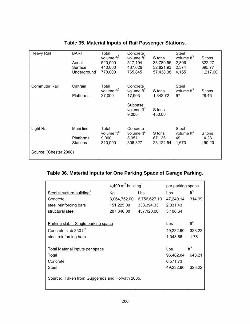
206
Table 35. Material Inputs of Rail Passenger Stations.
Heavy Rail BART Total Concrete Steel volume ft3 volume ft3 S tons volume ft3 S tons Aerial 520,000 517,194 38,789.56 2,806 822.27 Surface 440,000 437,626 32,821.93 2,374 695.77 Underground 770,000 765,845 57,438.38 4,155 1,217.60 Commuter Rail Caltrain Total Concrete Steel volume ft3 volume ft3 S tons volume ft3 S tons Platforms 27,000 17,903 1,342.72 97 28.46 Subbase volume ft3 S tons 9,000 450.00 Light Rail Muni line Total Concrete Steel volume ft3 volume ft3 S tons volume ft3 S tons Platforms 9,000 8,951 671.36 49 14.23 Stations 310,000 308,327 23,124.54 1,673 490.20 Source: (Chester 2008)
Table 36. Material Inputs for One Parking Space of Garage Parking.
4,400 m2 building1 per parking space
Steel structure building1 Kg Lbs Lbs ft3 Concrete 3,064,752.00 6,756,627.10 47,249.14 314.99steel reinforcing bars 151,225.00 333,394.33 2,331.43 structural steel 207,346.00 457,120.06 3,196.64 Parking slab – Single parking space Lbs ft3
Concrete slab 330 ft2 49,232.90 328.22steel reinforcing bars 1,043.66 1.78 Total Material inputs per space Lbs ft3 Total 96,482.04 643.21Concrete 6,571.73 Steel 49,232.90 328.22
Source:1 Taken from Guggemos and Horvath 2005.

207
Parking garages are complicated by the addition of a structure. Chester (Chester 2008) models parking garages as steel structures based on Guggemos and Horvath (Guggemos, Horvath 2005). The latter study compares environmental impacts between steel and concrete framed buildings. We model parking garages as a skeletal steel framed building with a reinforced concrete slab and nothing else. Guggemos and Horvath postulate two buildings, one is concrete framed and the other is steel framed. Both buildings have an area of 4,400 cubic meters spread over five stories. From Guggemos and Horvath we take the structural steel and reinforced concrete implied in a steel framed building and add a 12 inch reinforced concrete slab that has 330 square feet for every parking space. A 500 space lot has 165,000 square feet of area. Table 36 shows the calculations of material inputs per parking space in a parking garage. We begin with the material inputs based on Guggemos and Horvath’s 4,400 square meter steel framed building. Metric weight and area units are converted to US standard. The area of the hypothetical building would accommodate roughly 143 parking spaces. The structural material inputs are divided by 143 to obtain the structural material inputs per parking space. Concrete is converted to cubic feet assuming density of 150 lbs per cubic foot. We then add 330 square feet of 12 inch reinforced concrete slab using a default ratio of steel to concrete to obtain the total estimate. Estimation of Material and Electricity Emission Factors
Previous work reproduced here, has established greenhouse gas (GHG) emission factors for steel, aluminum, cement and concrete, asphalt concrete and coating materials, aggregate, process fuels solvents and lubricants, limited plastics, and equipment inputs. These emission factors include upstream and direct emissions for CO2, CH4, and N2O. Emission factors for materials are stated as grams of GHG per unit weight of material supplied. New emission factors are presented for brick, copper, wood and pressure treated wood, as these are commonly used in rail systems. We attempt to account for all GHG emissions that occur during the lifetime of the material from extraction to disposal. Process fuels are used in the production of the materials. We account for all stages of process fuels including extraction, transportation, refining, delivery, and combustion. Process emissions such as calcination of lime in cement making are accounted for as are fugitive emissions from such things as fuel or solvent evaporation or HFC leakage from cooling systems. Our model does substantially less well at accounting for downstream emissions. Emission factors for specific process fuels are presented in Table 37 which is based primarily on the GREET Model developed by Argonne National Laboratory (Argonne National Laboratory 2009, Argonne National Laboratory 2007). Emission factors are presented as grams per million Btu (MMBtu). The GREET Model allows for the conversion of emission factors for fuels from an energy content basis a weight or volume basis and vice versa using lower heating values (LHV) or higher heating values

208
(HHV). Life cycle analyses (LCA) were sought that provide the provide process fuel information.
Table 37. GHG Emissions of Process Fuels in g/MMBtu.
Upstream Emissions of Process Fuels (g/MMBtu)
Coal1 Natural Gas1
Conv. Gasoline1
Distillate Fuel Oil1
Residual Oil3 LPG1 Petroleum
Coke2 CO2 1,648 12,693 16,812 15,487 7,326 9,195 22,427 CH4 119.20 199.10 108.74 104.52 37.23 115.28 127.68 N2O 0.0313 0.2610 1.1400 0.2483 0.1179 0.1583 0.3866 Combustion Emissions of Process Fuels (g/MMBtu)
Coal1 Natural Gas1
Conv. Gasoline1
Distillate Fuel Oil1
Residual Oil1
LPG1
(Propane) Petroleum Coke1
CO2 108,363 59,379 75,645 78,169 85,045 68,024 104,716 CH4 4.00 1.10 5.19 0.18 3.24 1.08 4.00 N2O 1.0000 1.1000 2.4000 0.3900 0.3600 4.8600 1.0000 Upstream and Combustion Emissions of Process Fuels Combined (g/MMBtu)
Coal2 Natural Gas2
Conv. Gasoline2
Distillate Fuel Oil2
Residual Oil2
LPG2
(Propane) Petroleum Coke2
CO2 110,012 72,072 92,457 93,656 92,370 77,218 127,143 CH4 123.20 200.20 114 104.70 40.47 116.36 131.68 N2O 1.0313 1.3610 3.5400 0.6383 0.4779 5.0183 1.3866 Sources: 1. GREET Fuel Cycle Model 1.8c (Argonne National Laboratory 2009). 2. Our Calculations for Crude Extraction and Refining Share - energy basis from Fuel Cycle model and Summation of Combined Emissions.
Table 38 shows the materials identified as components of a rail system with emission factors expressed as tonnes of GHG per short ton of material. The basis for these emission factors are documented below. Some materials, notably aluminum, glass, lubricating oil, plastic and steel were taken directly from the GREET Vehicle Cycle Model (Argonne National Laboratory 2007). These emissions factors were expressed as grams of GHG per short ton in the GREET Model. The GREET Model provides combined emission factors for steel but provides separate emission factors for virgin and recycled aluminum. Emissions of GHG from electricity are expressed as tonnes per MWh using default assumptions from the GREET Fuel Cycle Model (Argonne National Laboratory 2009) assuming the default mix of process fuels used in the United States. Emissions based on the mix of process fuels used in the United States are higher than those based on the Northeastern US mix. The United States mix was chosen because it better represents US transit systems.
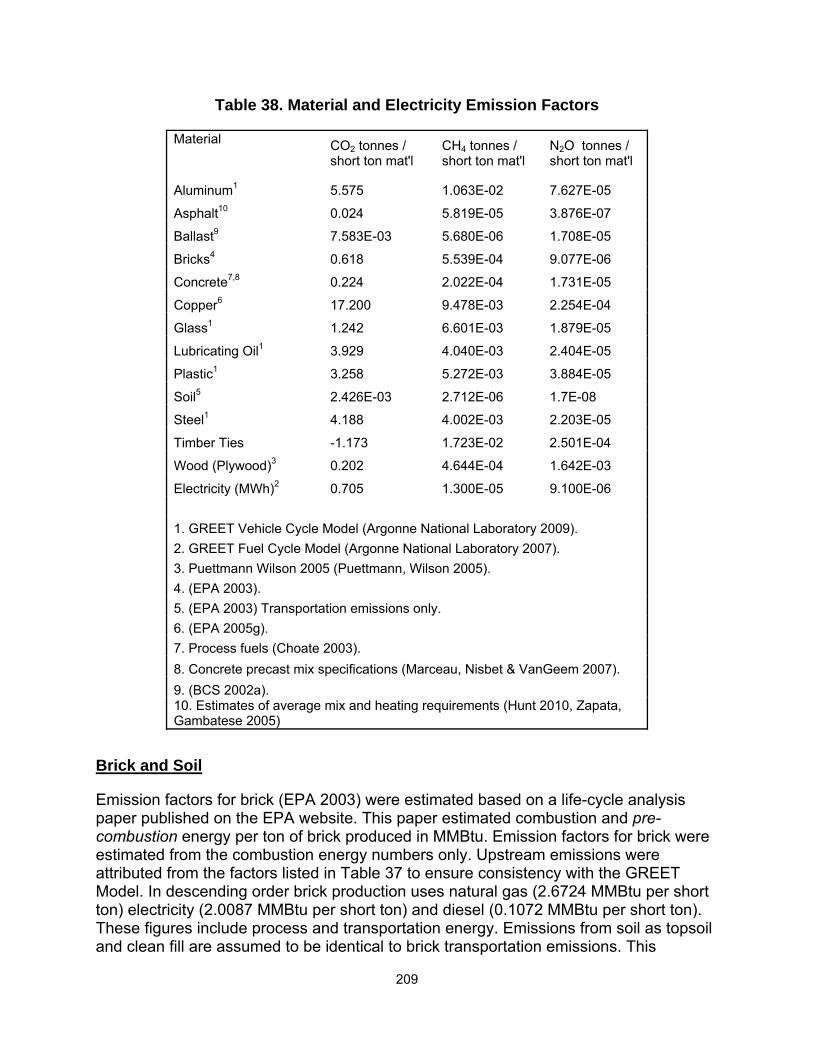
209
Table 38. Material and Electricity Emission Factors
Material CO2 tonnes / short ton mat'l
CH4 tonnes / short ton mat'l
N2O tonnes / short ton mat'l
Aluminum1 5.575 1.063E-02 7.627E-05
Asphalt10 0.024 5.819E-05 3.876E-07
Ballast9 7.583E-03 5.680E-06 1.708E-05
Bricks4 0.618 5.539E-04 9.077E-06
Concrete7,8 0.224 2.022E-04 1.731E-05
Copper6 17.200 9.478E-03 2.254E-04
Glass1 1.242 6.601E-03 1.879E-05
Lubricating Oil1 3.929 4.040E-03 2.404E-05
Plastic1 3.258 5.272E-03 3.884E-05
Soil5 2.426E-03 2.712E-06 1.7E-08
Steel1 4.188 4.002E-03 2.203E-05
Timber Ties -1.173 1.723E-02 2.501E-04
Wood (Plywood)3 0.202 4.644E-04 1.642E-03
Electricity (MWh)2 0.705 1.300E-05 9.100E-06 1. GREET Vehicle Cycle Model (Argonne National Laboratory 2009). 2. GREET Fuel Cycle Model (Argonne National Laboratory 2007). 3. Puettmann Wilson 2005 (Puettmann, Wilson 2005). 4. (EPA 2003). 5. (EPA 2003) Transportation emissions only. 6. (EPA 2005g). 7. Process fuels (Choate 2003). 8. Concrete precast mix specifications (Marceau, Nisbet & VanGeem 2007). 9. (BCS 2002a). 10. Estimates of average mix and heating requirements (Hunt 2010, Zapata, Gambatese 2005)
Brick and Soil
Emission factors for brick (EPA 2003) were estimated based on a life-cycle analysis paper published on the EPA website. This paper estimated combustion and pre-combustion energy per ton of brick produced in MMBtu. Emission factors for brick were estimated from the combustion energy numbers only. Upstream emissions were attributed from the factors listed in Table 37 to ensure consistency with the GREET Model. In descending order brick production uses natural gas (2.6724 MMBtu per short ton) electricity (2.0087 MMBtu per short ton) and diesel (0.1072 MMBtu per short ton). These figures include process and transportation energy. Emissions from soil as topsoil and clean fill are assumed to be identical to brick transportation emissions. This
210
estimate does not account for the equipment used to extract, load and unload soil. However, soil emissions are not considered in this model. They are rather used to derive equipment and transportation factors input. Copper and Aluminum
A similar process was used to estimate emissions from production and transportation of virgin and recycled copper wire. Embodied energy was estimated from a copper LCA paper (EPA 2005g). That paper includes estimates for all fuel types of energy inputs in MMBtu and GWP expressed as metric tons carbon equivalent (MTCE) per MMBtu for combustion CO2 and fugitive CH4. MTCE may be converted to GWP by dividing by the carbon fraction of CO2 (12/44). Electricity is the largest source of energy consumption used in virgin (61.2%) and recycled (53.2%) copper wire production followed by natural gas (virgin 36.0%, recycled 39.9%). Our calculations of emissions based on energy inputs were consistently higher than those in the EPA LCA paper because the latter used a source that did not account for upstream emissions from process fuels. Copper is a convoluted, energy-intensive, and specifically electricity-intensive process for both virgin and recycled copper wire. Electricity use drastically increases GHG emissions because it uses process fuels, which adds a step to energy production with a necessary loss of efficiency. Although the model’s estimated GHG emission factors are quite high they are not inconsistent with estimates from the GREET model. Emission factors for aluminum are taken directly from the GREET Vehicle Cycle Model (Argonne National Laboratory 2007). As with copper above, the GREET Model estimates GHG emissions for virgin and recycled aluminum. The United States Geological Survey compiles primary and secondary production numbers for many materials including aluminum (Buckingham, Plunkert & Bray 2010) and copper (Edelstein 2011). Recycled metals accounted for 61.1% of aluminum production in 2009 and 16.3% of copper production in 2010. These proportions were used to weight the virgin and recycled emission factors for both metals. Steel is weighted within the GREET Vehicle Cycle Model. Wood as Plywood
Emission factors for wood are taken from Puettmann and Wilson (Puettmann, Wilson 2005). They provide energy input from process fuels for plywood and other wood products that do not lend themselves to estimation of upstream GHG emissions as done in the GREET model. Emission factors were based on the authors’ estimation of GHG emissions despite the fact that those estimates do not include upstream emissions from fossil fuels. For our model this was corrected by adding upstream emissions based on the reported energy from fossil fuels based on the GREET model--roughly half of the energy consumed in plywood production--to the estimates. We added emissions from process fuels including coal and natural gas as upstream emissions. Upstream emissions for crude oil were substituted for residual oil, which results in a slight overestimation. This overestimation is offset by omitted upstream emissions from uranium, hydropower, and a quite small amount of electricity. Any overestimation of
211
GHG emissions is exacerbated by omission of a credit for an upstream biomass GWP sink. Plywood was chosen as the basis for wood emission factor for stations. Concrete
Emission factors for concrete were established from Choate (Choate 2003). Table 39 is based on the fuel inputs reported in that paper using emission factors for process fuels reported above. It shows direct and upstream emissions of GHGs assuming a wet concrete mixture of 12% cement, 82% aggregate, and 6% water. This method allows for adjustment to differences in mix specifications. The concrete industry’s LCA analysis (Marceau, Nisbet & VanGeem 2007) does not allow these adjustments. The adjustment process is straightforward with a known mix. All emissions from quarrying are divided by 82. Those from cement are divided by 12. Concrete manufacturing emissions are not adjusted. The result is a series of factors that will allow a user to estimate the GHG emissions of any mix specified in percentages. We assume that concrete is a typical precast made from a mix that is 16.41% cement, 77.02% aggregate, and 6.57% water. Emissions from aggregate are taken from an analysis of fuel consumption from limestone and crushed rock extraction (BCS 2002a). Greenhouse gas emissions are attributed based on the emission factors shown in Table 39. We assume that emission factors are the same for limestone, aggregate, and ballast rock. Asphalt
This section is an abbreviated version of work we did previously. We assume an average mix for hot mix asphalt of 5% binder and 95% aggregate with moisture content of 4% in the aggregate (Zapata, Gambatese 2005). Upstream emissions of aggregate are taken from BCS (BCS 2002a). The upstream emissions from binder are similar to those from residual oil. We correct on an energy basis using LHV and refinery efficiencies based on Wang (Wang 2008). We estimate the heating requirement based on the specific heat of binder, aggregate, water and steam, and the latent heat required to convert water into steam (Hunt 2010). We then correct for imperfect heating efficiency using an average energy consumption estimate from Zapata et al. (VTC 2010). Creosote Treated Timber
The life cycle of timber railroad ties includes four stages including production of green cut timbers, pressure treatment of timbers with creosote, active life and disposal. Smith and Bolin (Smith, Bolin 2010) address all four of these stages however we amend some of their assumptions to make our approach to timber ties consistent with other emission factors presented here. First, Smith and Bolin assume that the green timber contributes no GHG emissions because the carbon in it results from recent photosynthesis and not fossilized hydrocarbons. While the assumption is correct, this approach discounts emissions associated with harvesting, cutting and air drying the timber, and transportation. This error is corrected by supplementing from the life cycle analysis
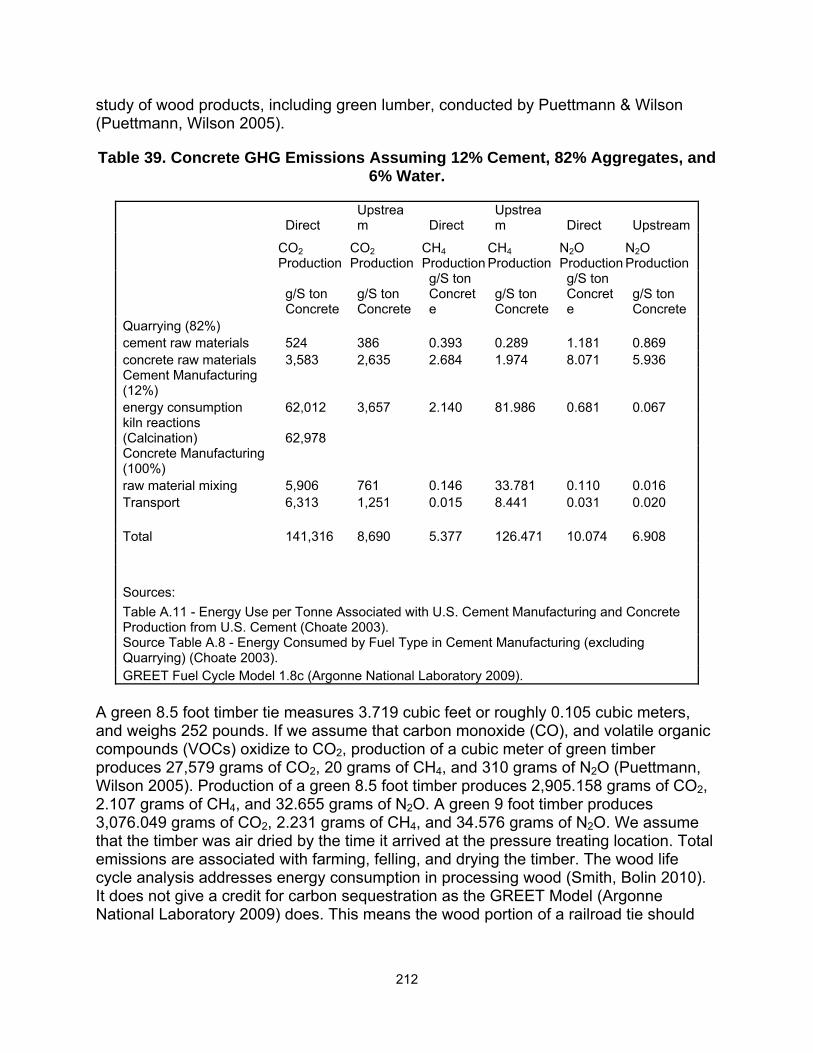
212
study of wood products, including green lumber, conducted by Puettmann & Wilson (Puettmann, Wilson 2005).
Table 39. Concrete GHG Emissions Assuming 12% Cement, 82% Aggregates, and 6% Water.
Direct Upstream Direct
Upstream Direct Upstream
CO2 Production
CO2 Production
CH4 Production
CH4 Production
N2O Production
N2O Production
g/S ton Concrete
g/S ton Concrete
g/S ton Concrete
g/S ton Concrete
g/S ton Concrete
g/S ton Concrete
Quarrying (82%) cement raw materials 524 386 0.393 0.289 1.181 0.869 concrete raw materials 3,583 2,635 2.684 1.974 8.071 5.936 Cement Manufacturing (12%) energy consumption 62,012 3,657 2.140 81.986 0.681 0.067 kiln reactions (Calcination) 62,978 Concrete Manufacturing (100%) raw material mixing 5,906 761 0.146 33.781 0.110 0.016 Transport 6,313 1,251 0.015 8.441 0.031 0.020 Total 141,316 8,690 5.377 126.471 10.074 6.908
Sources: Table A.11 - Energy Use per Tonne Associated with U.S. Cement Manufacturing and Concrete Production from U.S. Cement (Choate 2003). Source Table A.8 - Energy Consumed by Fuel Type in Cement Manufacturing (excluding Quarrying) (Choate 2003). GREET Fuel Cycle Model 1.8c (Argonne National Laboratory 2009).
A green 8.5 foot timber tie measures 3.719 cubic feet or roughly 0.105 cubic meters, and weighs 252 pounds. If we assume that carbon monoxide (CO), and volatile organic compounds (VOCs) oxidize to CO2, production of a cubic meter of green timber produces 27,579 grams of CO2, 20 grams of CH4, and 310 grams of N2O (Puettmann, Wilson 2005). Production of a green 8.5 foot timber produces 2,905.158 grams of CO2, 2.107 grams of CH4, and 32.655 grams of N2O. A green 9 foot timber produces 3,076.049 grams of CO2, 2.231 grams of CH4, and 34.576 grams of N2O. We assume that the timber was air dried by the time it arrived at the pressure treating location. Total emissions are associated with farming, felling, and drying the timber. The wood life cycle analysis addresses energy consumption in processing wood (Smith, Bolin 2010). It does not give a credit for carbon sequestration as the GREET Model (Argonne National Laboratory 2009) does. This means the wood portion of a railroad tie should
213
not contribute to GHG emissions so Smith and Bolin consider only emissions from the creosote. Because Smith and Bolin do not estimate energy consumed in the pressure treating process or fugitive emissions resulting from evaporation, we cannot either. Most commercial creosote wood preservative products are diluted with solvents (IPCS 2004). As a result uncontrolled fugitive emissions may be substantial. The pressure treating process results in the loss of some of the water in the timber and addition of creosote (Smith, Bolin 2010). An 8.5 foot (102 inches) untreated tie weighs roughly 252 lbs of which 148 lbs are dry mass or 0.074 tons. The water weight of a green timber tie is 104 lbs. Coal tar creosote is a distillate of coal tar that is composed of aromatic hydrocarbons of a variety of densities, but lacking the heaviest materials found in coal tar (Agency for Toxic Substances and Disease Registry 2010)(Agency for Toxic Substances and Disease Registry 2010)(Agency for Toxic Substances and Disease Registry 2010). Coal tar is a byproduct of carbonization of coal to produce metallurgical coke or natural gas for gasification. The pressure treating process reduces the water weight of the tie to 59 lbs and adds 20 lbs of creosote to t(Agency for Toxic Substances and Disease Registry 2010)(Agency for Toxic Substances and Disease Registry 2010)he tie. The carbon weight of the creosote is 10.637 lbs94, so that the carbon fraction estimate of creosote is 0.818 (Smith, Bolin 2010). This is somewhat low but not unreasonable for solvent-diluted aromatic (cyclic) hydrocarbons with some minor replacement of carbon with oxygen, nitrogen, sulfur, and similar radicals found in such compounds as tar acids and bases, aromatic amines, phenolics, and nitrogen, sulfur, and oxygen heterocycles that make up 10% or slightly more of the weight of undiluted coal tar creosote (IPCS 2004). As 7 lbs of creosote are outgassed per tie, the resulting CO2 would weigh 9,525 grams if all of the carbon is outgassed as CO2 (Smith, Bolin 2010). This approach has some gaps. Smith and Bolin assume that all decayed wood and lost creosote are released as VOCs, CO or CO2 and that the non-CO2 components quickly oxidize to CO2 in the atmosphere (Smith, Bolin 2010). This assumption probably ignores a small amount of CH4 and N2O emissions from the wearing of timber ties. It also ignores scientific evidence that a significant part of commercial creosote solutions used as wood preservatives are released in rain runoff and not into the atmosphere (Tran et al. 2009). Therefore, these are minor shortcomings in our knowledge of creosote emissions. Smith and Bolin (Smith, Bolin 2010) estimate emissions for two disposal scenarios: recycling as fuel, and landfill disposal. Each tie offsets 1.4 million Btu (MMBtu) of energy from coal. It is assumed in the GREET Model (Argonne National Laboratory 2009) that combined upstream and direct emissions from burning 1.4 MMBtu of coal are 154,017 grams of CO2, 172.480 grams of CH4, and 1.444 grams of N2O. These are the emissions that are saved as a result of burning used railroad ties instead of coal. Combustion of the wood in the ties is assumed to be carbon neutral since it is not fossil based. The 13 pounds of creosote remaining at the end of the service life of a railroad tie produce 17,690 grams of CO2. Smith and Bolin assume no 94 39 * 12 / 44 = 10.637 where 12 / 44 is the proportion of CO2 made up of Carbon by weight.
214
CH4 or N2O emissions from combustion of creosote, or wood. Based on our interpretation of this model, net emissions from burning used railroad ties as fuel is -136,327 grams of CO2, -172.480 grams of CH4, and -1.444 grams of N2O. Smith and Bolin (Smith, Bolin 2010) estimate CO2 and CH4 emissions for landfill disposal at 3,175 grams of fossil CO2 and 2,354 grams of CH4. These emissions are offset by 3.0 lbs or 1360.776 grams of captured natural gas, which could be used as fuel. Natural gas has a lower heating value of 983 Btu per cubic foot and a density of 22 grams per cubic foot. The fuel offset would produce 0.060802 MMBtu of heat and save 72,072 grams of CO2 emissions, 200.20 grams of CH4 emissions, and 1.361 grams of N2O emissions. Smith and Bolin do not account for carbon sequestration of the wood portion of the railroad tie. They state that 77% of the ties’ mass remains in the earth for an extended period. By applying this fraction to the dry weight of the wood in the used tie we obtain a result of 108.57 pounds or 49,247 grams. If we adopt a commonly used benchmark for carbon fraction of dry wood of 0.5 (Lamlon, Savidge 2006) the carbon content of the wood portion of a used tie is 24,624 grams, which would produce 90,288 grams of CO2 sequestration. We estimate that net emissions from sending used railroad ties to the landfill are -159,185 grams of CO2, 2,154 grams of CH4, and -1.361 grams of N2O. Smith and Bolin state that the purpose of their analysis is to compare differences in GHG emissions between two alternative approaches to disposal. As a result they do not intend to present a full life cycle analysis, they leave upstream emissions out of the analysis. We add upstream emissions from another source for wood and assume that as a byproduct of coal and coke production coal tar creosote has no upstream GHG emissions. This assumption neglects the upstream emissions of solvents used to cut creosote for wood preservation. Another gap is that there is no treatment of energy consumption or fugitive emissions in the pressure treating process. We assume that emissions during the service life consist only of the carbon content of fugitive emissions that are outgassed as CO2. The CH4 emissions from solvents are likely to be quite small and a N2O component is likely non-existent. The large net savings with either disposal method are probably valid given the large fuel credits for coal substitution and the large credits for landfill sequestration of carbon in wood. However Smith and Bolin do not address CH4 and N2O emissions from combustion. Table 40 summarizes emission factors for one cubic foot of timber rail tie. Smith and Bolin (Smith, Bolin 2010) recommend that ties be recycled as fuel at the end of their service life, which could provide an offset to other fuels. That study is biased against landfill disposal because it does not account for carbon sequestration in landfills. Carbon sequestration in landfills was our adjustment to the model. Although they cite EPA sources for their estimation of methane production in landfills, we have not looked at their work in depth. However, the methane levels they claim are quite high and bare further investigation. For our analysis we will assume that timber ties are disposed of in landfills.

215
Table 40. GHG Emission Factors for Creosote Pressure Treated Timber Railroad Ties
CO2 CH4 N2O GWP g/ft3 g/ft3 g/ft3 Upstream Emissions 781 0.567 8.781 3,515 Pressure Treating 0 0 0 0
Fugitive Emissions 2,561 0 0 2,561 Disposal Use as Fuel -36,656 -46.378 -0.388 -37,751 Landfill -42,803 579.188 -0.366 -30,754 Total Fuel -33,314 -45.812 8.392 -31,674 Landfill -39,461 579.755 8.415 -24,677
Conclusion and Summary
Table 41 shows updated Emission factors for all rail system components. Overhead line equipment, tunnels, bridges, and rolling stock are taken from Network Rail (Network Rail ). Rail stations and parking facilities are taken from Chester (Chester 2008) except for parking garages, which are based largely on Guggemos and Horvath (Guggemos, Horvath 2005) for the building structure and our conversion of Chester’s flexible pavement to a rigid slab for the parking surface. We have added GHG emission factors for copper in order to adequately address catenary wire systems. By weight catenary wire systems have about one sixth as much copper as they have steel, yet the GHG emissions from copper wire production and rolled steel production are roughly equivalent. The catenary systems are massive with steel content larger than 132 pound track on reinforced concrete ties. Our model assumes 887 tons of steel per route-mile for catenary systems and 582 tons per route-mile for 132 pound track. Other additions include wood as plywood and pressure treated timber, glass, lubricating oil, brick and soil. We cannot precisely estimate from the bottom up for many factors including catenary wires, bridges, tunnels, rolling stock,passenger stations or parking garages. It was designed to address the type of data likely to be available from transit agencies. Our analysis of a case-study for Denver (as part of TCRP H41) found that it included counts of miles of track, vehicles of rolling stock, primary hub rail stations and secondary feeder stations, and parking spaces for parking lots and parking garages.
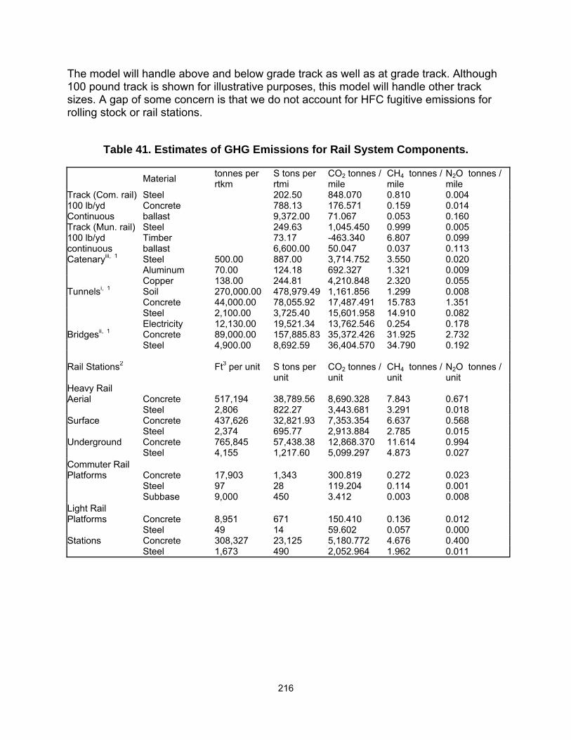
216
The model will handle above and below grade track as well as at grade track. Although 100 pound track is shown for illustrative purposes, this model will handle other track sizes. A gap of some concern is that we do not account for HFC fugitive emissions for rolling stock or rail stations.
Table 41. Estimates of GHG Emissions for Rail System Components.
Material tonnes per rtkm
S tons per rtmi
CO2 tonnes / mile
CH4 tonnes / mile
N2O tonnes / mile
Track (Com. rail) Steel 202.50 848.070 0.810 0.004 100 lb/yd Concrete 788.13 176.571 0.159 0.014 Continuous ballast 9,372.00 71.067 0.053 0.160 Track (Mun. rail) Steel 249.63 1,045.450 0.999 0.005 100 lb/yd Timber 73.17 -463.340 6.807 0.099 continuous ballast 6,600.00 50.047 0.037 0.113 Catenaryiii, 1 Steel 500.00 887.00 3,714.752 3.550 0.020 Aluminum 70.00 124.18 692.327 1.321 0.009 Copper 138.00 244.81 4,210.848 2.320 0.055 Tunnelsi, 1 Soil 270,000.00 478,979.49 1,161.856 1.299 0.008 Concrete 44,000.00 78,055.92 17,487.491 15.783 1.351 Steel 2,100.00 3,725.40 15,601.958 14.910 0.082
Electricity 12,130.00 19,521.34 13,762.546 0.254 0.178 Bridgesii, 1 Concrete 89,000.00 157,885.83 35,372.426 31.925 2.732 Steel 4,900.00 8,692.59 36,404.570 34.790 0.192 Rail Stations2 Ft3 per unit S tons per
unit CO2 tonnes / unit
CH4 tonnes / unit
N2O tonnes / unit
Heavy Rail Aerial Concrete 517,194 38,789.56 8,690.328 7.843 0.671 Steel 2,806 822.27 3,443.681 3.291 0.018 Surface Concrete 437,626 32,821.93 7,353.354 6.637 0.568 Steel 2,374 695.77 2,913.884 2.785 0.015 Underground Concrete 765,845 57,438.38 12,868.370 11.614 0.994 Steel 4,155 1,217.60 5,099.297 4.873 0.027 Commuter Rail Platforms Concrete 17,903 1,343 300.819 0.272 0.023 Steel 97 28 119.204 0.114 0.001 Subbase 9,000 450 3.412 0.003 0.008 Light Rail Platforms Concrete 8,951 671 150.410 0.136 0.012 Steel 49 14 59.602 0.057 0.000 Stations Concrete 308,327 23,125 5,180.772 4.676 0.400 Steel 1,673 490 2,052.964 1.962 0.011

217
Table 41. Non-Track Estimates of GHG Emissions--Continued.
Parking Facilities Material Ft3 per parking space
S tons per parking space
CO2 tonnes / parking space
CH4 tonnes / parking space
N2O tonnes / parking space
Parking Garage2,3 Concrete 48.24 10.808 0.010 8.35 x 10⁻⁴ Steel 3.29 13.761 0.013 7.2 x 10⁻⁵ Total 330 51.53 24.569 0.023 9.07 x 10⁻⁴ Parking Lot2 Hot Mix Asphalt 165 7.69 0.187 4.47 x 10⁻⁴ 3 x 10⁻⁶ Aggregate 165 8.25 0.063 4.7 x 10⁻⁵ 1.41 x 10⁻⁴ Total 330 15.94 0.250 4.94 x 10⁻⁴ 1.44 x 10⁻⁴
Rolling Stock1 Material tonnes per vehicle
S tons per vehicle
CO2 tonnes / vehicle
CH4 tonnes / vehicle
N2O tonnes / vehicle
Steel 27.05 29.82 124.876 0.119 6.57 x 10⁻⁴ Aluminum 12.60 13.89 77.435 0.148 0.001 Copper 1.20 1.32 22.752 0.013 2.98 x 10⁻⁴ Glass 0.82 0.90 1.122 0.006 1.7 x 10⁻⁵ Lubricating Oil 0.63 0.69 2.729 0.003 1.7 x 10⁻⁵ Wood (Plywood) 1.45 1.60 0.354 0.002 0.002
Plastic and Rubber 3.43 3.78 12.317 0.020 1.47 x 10⁻⁴
i. per unit distance of tunnels ii. per unit distance of bridges iii. per unit distance of track Sources: 1. Network Rail. n.d. Comparing Environmental Impact of Conventional and High Speed Rail. 2. Chester. 2008. Life-Cycle Environmental Inventory of Passenger Transportation in the United States. 3. Guggemos, A.A.; Horvath, A. 2005. Comparison of Environmental Effects of Steel- and Concrete-Framed Buildings. An important limitation of the model is that we often do not account for equipment activity. Where we have this information it is through the LCA studies we cite. The Choate study (Choate 2003) on concrete and the BCS study (BCS 2002a) on aggregate and ballast account for equipment activity fairly well, although their assumptions may be outdated. Our asphalt assumptions are based on a heating model (Hunt 2010) and industry averages (Zapata, Gambatese 2005). Direct equipment emissions are accounted for abstractly in these cases. The GREET Model (Argonne National Laboratory 2009, Argonne National Laboratory 2007) would address equipment activity data at least as well these other models already mentioned, except that it does not address installation of materials by a contractor. Where we do not account for activity well at all is where there is no LCA or only a poor LCA available. The EPA reports for copper and brick (EPA 2003, EPA 2005g) do not address upstream emissions completely. We use GREET process fuel emission factors from Table 37 to correct for this. Again, we do not address installation of these materials. The wood study (Puettmann, Wilson 2005) addresses upstream equipment but like GREET, it does not address installation. We do not have activity data for track installation, building

218
construction, or demolition. A similar limitation is that we do not address disposal or recycling and the end of the life cycle.
219
APPENDIX H: GASCAP CASE STUDIES
Introduction
This section summarizes four case studies based on inputting DOT bid sheet information into GASCAP. Various assumptions were made to estimate equipment activity. We identify various omissions in GASCAP and potential procedures for use of the software. The results, however, are indicative of the variation in emissions that different projects will produce. We establish the inputs for each contract based on the item numbers in the bid sheets. Some item numbers are excluded from the analysis for a variety of reasons. These items include administrative components, including the development and management of development and management of construction layouts and progress schedules, testing procedures, setting up and maintaining a field office, price adjustments, and obtaining the required performance and payment bonds and liability insurance are excluded. Training activities are noted but not quantified. Temporary reusable items such as breakaway barricades, cones, drums, and construction signs and other temporary signage are also not included, as are services such as towing or use of traffic directors. Material inputs do not include Division 700 – Electronics and Division 800 – Landscaping. Many of these items either have no impact on greenhouse gas emissions (e.g. liability insurance) or are minor. Further research can develop procedures for additional bid sheet items, if needed. Equipment activities are included indirectly. Some equipment activities are noted explicitly such as site clearing, excavation, concrete and hot mix asphalt (HMA) milling, and final cleanup. Other examples include saw cutting, setting of materials accounted for elsewhere, such as inlets, and pile driving. Other equipment activities are implied by material inputs such as laying concrete, paving, spraying, and placing structures. There are no specifics in the bid sheets about mobilization, which is generally covered as a lump sum. We make an attempt to estimate equipment activity input from the contract items, but must make assumptions about specifically what equipment is used, the duration of use, the power rating, and the fuel used by the equipment. Staging and lighting assumptions are made in a similar way. Some assumptions are made to demonstrate the Recyclables module for contracts 135083070 and 003048072. Other than as described above, material inputs are discussed with a focus on which materials are included and which are missing. Omissions are discussed in some detail. Quantified greenhouse gas emissions are presented for each module in tabular form. Following this introduction, each contract is presented. GASCAP output is then attached for each contract followed by the best three bids for each contract from the bid-sheets for reference.

220
Contract 001093740: Grove Street (CR623) over Route 46, Clifton City, Passaic County
This contract addresses road and bridge reconstruction where Grove Street, Clifton, Passaic County passes over NJ Route 46 at milepost 61.09. The contract was awarded 7/23/2009 with a scheduled completion date of 11/19/2009. If we assume that work on the project begins on the let date the project’s duration is 119 days. We assume that all work is completed during daylight hours. The roadway component of this project uses soil aggregate, aggregate subbase and a concrete base course all expressible in cubic yards. Roughly 600 square yards of existing HMA pavement is milled to a depth of 3 inches. A tack coat is applied, which is presumed not to include cutback agents. HMA intermediate and surface courses are applied, accounting for 340 tons of material. HMA and concrete sidewalks and an HMA driveway of known depth are presented in square yards. A concrete vertical curve of known height and thickness and ductile water pipe of known diameter are presented in linear feet. Epoxy traffic stripes are not included. A temporary chain link fence is not included because it is presumed to be reusable. A fire hydrant could not be included as this item is not in GASCAP. A gas main including bridge and non-bridge components were included as were backfilling, bedding, and installation using coarse aggregate. The bridge component includes concrete wing walls, abutment walls, pier column and cap, and bridge deck expressed in cubic yards, and epoxy-coated reinforcement steel expressed in pounds. Concrete bridge sidewalk and parapet are expressed in linear feet. Structural steel is expressed as a lump sum. We allow 50,000 pounds for structural steel. A permanent chain-link aluminum-coated steel fence of known height is expressed in linear feet. Missing items include temporary shielding and sheeting, epoxy waterproofing, reinforced elastomeric bearing assembly units, shear connectors, and strip seal expansion joint assemblies. An item for 100 square feet of concrete repair could not be addressed because it is not in GASCAP. An erosion control system including silt fencing, inlet filters, concrete washout systems and an oil only emergency spill kit are not covered. Landscaping including topsoiling, fertilizing and seeding, and straw mulching was also not covered. In addition to site clearing and final clean up, equipment activity includes 198 cubic yards of unclassified excavation and 75 cubic yards of gas line excavation, 606 square yards of HMA milling to a depth of three inches, 75 square yards of underlayer preparation, resetting of 2 castings, one manhole, one gas valve box, removal of erosion control sediment, various HMA and concrete paving and pavement repairs, and various installations. Cleaning of 495 feet of pipe and 8 drains is noted. Training activities consisting of 28,000 hours of training are noted as well.
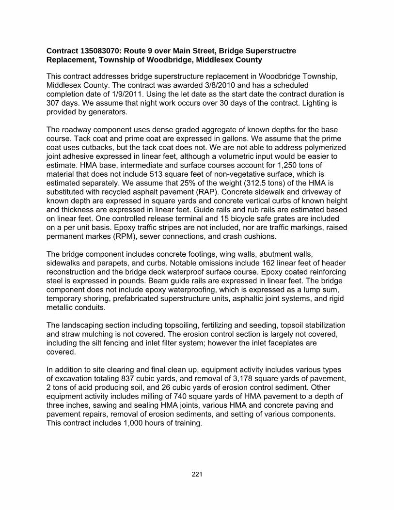
221
Contract 135083070: Route 9 over Main Street, Bridge Superstructre Replacement, Township of Woodbridge, Middlesex County
This contract addresses bridge superstructure replacement in Woodbridge Township, Middlesex County. The contract was awarded 3/8/2010 and has a scheduled completion date of 1/9/2011. Using the let date as the start date the contract duration is 307 days. We assume that night work occurs over 30 days of the contract. Lighting is provided by generators. The roadway component uses dense graded aggregate of known depths for the base course. Tack coat and prime coat are expressed in gallons. We assume that the prime coat uses cutbacks, but the tack coat does not. We are not able to address polymerized joint adhesive expressed in linear feet, although a volumetric input would be easier to estimate. HMA base, intermediate and surface courses account for 1,250 tons of material that does not include 513 square feet of non-vegetative surface, which is estimated separately. We assume that 25% of the weight (312.5 tons) of the HMA is substituted with recycled asphalt pavement (RAP). Concrete sidewalk and driveway of known depth are expressed in square yards and concrete vertical curbs of known height and thickness are expressed in linear feet. Guide rails and rub rails are estimated based on linear feet. One controlled release terminal and 15 bicycle safe grates are included on a per unit basis. Epoxy traffic stripes are not included, nor are traffic markings, raised permanent markes (RPM), sewer connections, and crash cushions. The bridge component includes concrete footings, wing walls, abutment walls, sidewalks and parapets, and curbs. Notable omissions include 162 linear feet of header reconstruction and the bridge deck waterproof surface course. Epoxy coated reinforcing steel is expressed in pounds. Beam guide rails are expressed in linear feet. The bridge component does not include epoxy waterproofing, which is expressed as a lump sum, temporary shoring, prefabricated superstructure units, asphaltic joint systems, and rigid metallic conduits. The landscaping section including topsoiling, fertilizing and seeding, topsoil stabilization and straw mulching is not covered. The erosion control section is largely not covered, including the silt fencing and inlet filter system; however the inlet faceplates are covered. In addition to site clearing and final clean up, equipment activity includes various types of excavation totaling 837 cubic yards, and removal of 3,178 square yards of pavement, 2 tons of acid producing soil, and 26 cubic yards of erosion control sediment. Other equipment activity includes milling of 740 square yards of HMA pavement to a depth of three inches, sawing and sealing HMA joints, various HMA and concrete paving and pavement repairs, removal of erosion sediments, and setting of various components. This contract includes 1,000 hours of training.

222
Contract 003048072: Route US 22 Resurfacing and County Route 519 Intersection Improvements, from Phillipsburg Mall Entrance to Vicinity of Greenwich
This contract addresses resurfacing of US Route 22 and intersection improvements to County Route 519 in Greenwich and Pohatcong Townships in Warren County. The contract was awarded 2/1/2011 and is scheduled for completion 9/12/2011. The time from let date to completion date is 223 days, which we assume to be the active phase of the contract. We assume that night work occurs throughout the contract. Lighting is provided by grid electricity. The roadway component includes dense-graded aggregate and concrete base courses of various depths, 12,920 gallons of tack and prime coat, 10,990 tons of HMA base, intermediate, and surface courses, 213 linear feet of reinforced concrete pipe, various inlets, a four foot manhole, curb pieces, a HMA driveway, concrete island, concrete vertical curbs, an HMA non-vegetative surface, various guide and rub rails, and signage. Not included were HMA pavement repair, 26,500 linear feet of polymerized joint adhesive, 8,100 linear feet of joint sealing in concrete pavement, epoxy traffic stripes, thermoplastic traffic markings, RPMs of various specifications, and a concrete handicap ramp. We assume substitution of recycled material in concrete including 50 cubic yards of RCM (7,500 lbs) and 50 lbs of coal fly ash. The bridge component of the project is limited to a caste-in-place retaining wall of 354 square feet. GASCAP does not include this item code. The erosion control component includes silt fencing, hay bales, inlet filters, concrete washout systems and oil emergency spill kits. The electronics component includes 135 linear feet of rigid metallic conduit, 1,737 linear feet of ground wire, foundations, and traffic signal boxes and mast arms of aluminum and steel. The landscaping component includes tree removal, topsoiling to various depths, turf application, fertilizing and seeding, mulching with hardwood bark, planting of ground cover and various itemized trees and shrubs, and building of a stone wall. These items and construction monuments are not covered by GASCAP. In addition to site clearing and final clean up, equipment activity includes 244 cubic yards of excavation, 670 square yards of pavement removal, HMA milling to various depths, various HMA and concrete paving and pavement repairs, pipe cleaning, and setting and resetting of various items. This contract had no provision for training. Contract 045093060: Route 1 & 9 North Avenue to Haynes Avenue Resurfacing, Mill and pave, City of Newark and Elizabeth (Essex and Union Counties)
This contract covers milling and paving of sites in Newark, Essex County and Elizabeth, Union County. The contract was awarded 2/8/2011 and has a scheduled completion date of 1/21/2012. As with the previous three contracts we assume that work began on the project let date and will continue until the completion date, which gives the project a
223
duration period of 347 days. We assume that all work is completed during daylight hours. This contract has no bridge component. The roadway component includes 3,628 cubic yards of subbase, 20,658 gallons of tack and prime coat, and more than 48,000 tons of HMA including 11,190 tons of binder rich intermediate course (Item No. 409003P). This last item was entered HMA intermediate course (Item No. 401066M) with binder content specified at 7%. This contract also includes three types of inlet, bicycle safe grates, curb pieces, inlet face plates, 160 square yards of four inch thick concrete island, concrete vertical curbs, and signage. Items not included were 194 square yards of HMA pavement repair, epoxy traffic stripes, thermoplastic traffic markings, RPMs and rumble strips. The erosion control component of this contract includes silt fencing, inlet filters of various types, a concrete washout system, and an oil emergency spill kit. The landscaping component includes topsoiling, fertilizing and seeding, and straw mulching. Beyond site clearing and final cleanup, equipment activities include excavation of 7,519 cubic yards, HMA and concrete milling to various depths of more than 175,000 square yards of pavement, paving and various HMA and concrete pavement repairs, erosion sediment removal, pipe and drain cleaning, and placing, setting, and installing various items. Training in this contract consists of 740 hours. Lessons learned from case studies
These case studies have demonstrated the capability and the shortcomings of GASCAP. Our estimates of greenhouse gas emissions likely cover about 90% of the total construction life-cycle emissions associated with these projects, assuming our assumptions on equipment activity are correct. The lack of detailed construction equipment activity is the major shortcoming, and there is a need to develop methods to estimate the equipment activity for a variety of projects. As part of GASCAP development, we included detailed specifications for over 1000 bid sheet items. Despite this, the case studies identified various omissions of bid sheet items that were missing from the bid lists we surveyed. One item also had inadequate information on size and dimensions to calculate a volumetric measure. Some items also are reported as lump sums making it impossible to disentangle the individual components of the item. DOT should consider requiring additional detail in bid sheets to allow a full estimation of the emissions from these items. GASCAP will benefit from feedback from DOT staff who begin to explore the capabilities of GASCAP. We recommend that missing items be identified as well as any other assumptions that are made while entering bid sheet items.

Results
SECTION 1: Materials OVERALL RESULTS
Direct CO2 7.13 (mt) CO2 5,758.73 (mt)Direct CH4 0.00 (mt) CH4 5.39 (mt)Direct N2O 0.00 (mt) N2O 0.80 (mt)Direct CO2 Equivalent 7.17 (mt) PMBC 0.01 (mt)Upstream CO2 5,686.34 (mt)
Upstream CH4 5.19 (mt) Total CO2 Equivalent 6,120.94 (mt)Upstream N2O 0.80 (mt)Upstream CO2 Equivalent 6,043.51 (mt) Fuel ConsumptionCombined CO2 Equivalent 6,050.68 (mt)
Gasoline (10% Ethanol RFG) 0.00 gallonsSECTION 2: Equipment Gasoline 740.07 gallons
20% Biodiesel 0.00 gallonsDirect CO2 50.23 (mt) Diesel 7,937.85 gallonsDirect CH4 0.00 (mt) Liquified Petroleum Gas 0.00 gallonsDirect N2O 0.00 (mt) Compressed Natural Gas 0.00 GGEDirect PMBC 0.01 (mt)Direct CO2 Equiv. from HFCs 0.00 (mt) Fuel CostsDirect CO2 Equivalent 50.45 (mt) Gasoline (10% Ethanol RFG) $ per gallonUpstream CO2 9.88 (mt) Gasoline $ per gallonUpstream CH4 0.19 (mt) 20% Biodiesel $ per gallonUpstream N2O 0.00 (mt) Diesel $ per gallonUpstream PMBC 0.00 (mt) Liquified Petroleum Gas $ per gallonUpstream CO2 Equivalent 14.00 (mt) Compressed Natural Gas $ per GGECombined CO2 Equivalent 64.45 (mt)
SECTION 3: Recyclables Credits
CO2 0.00 (mt) Total Fuel Cost $34,711.69CH4 0.00 (mt)N2O 0.00 (mt)Total CO2 Equivalent 0.00 (mt)
SECTION 4: Lifecycle Maintenance SECTION 5: Staging
Direct CO2 0.00 (mt) Direct CO2 4.28 (mt)Direct CH4 0.00 (mt) Direct CH4 0.00 (mt)Direct N2O 0.00 (mt) Direct N2O 0.00 (mt)Direct PMBC 0.00 (mt) Direct CO2 Equiv. from HFCs 0.46 (mt)Direct CO2 Equivalent 0.00 (mt) Direct CO2 Equivalent 4.80 (mt)Upstream CO2 0.00 (mt) Upstream CO2 0.87 (mt)Upstream CH4 0.00 (mt) Upstream CH4 0.01 (mt)Upstream N2O 0.00 (mt) Upstream N2O 0.00 (mt)Upstream PMBC 0.00 (mt) Upstream CO2 Equivalent 1.01 (mt)Upstream CO2 Equivalent 0.00 (mt) Combined CO2 Equivalent 5.81 (mt)Combined CO2 Equivalent 0.00 (mt)
SECTION 6: Lighting SECTION 7: Rail
Direct CO2 0.00 (mt) Direct CO2 0.00 (mt)Direct CH4 0.00 (mt) Upstream and Disposal CO2 0.00 (mt)Direct N2O 0.00 (mt) Upstream and Disposal CH4 0.00 (mt)Direct CO2 Equivalent 0.00 (mt) Upstream and Disposal N2O 0.00 (mt)
Total CO2 Equivalent 0.00 (mt)
NJDOT Contract Num 001093740 Contract ID 09151

Materials
Item Code Description Value Unit Cement Ratio Aggregate Ratio Heating Temp. % Binder % Moisture Cutback Depth (feet)
509078P Chain-Link Fence, Aluminum-Coated Steel, Bridge, 6' 3" 460.00 Feet N/A N/A N/A N/A N/A Non-Solvent-N/A N/A
507039P Concrete Bridge Parapet, Hpc 460.00 Feet 0.15 0.80 N/A N/A N/A Non-Solvent-N/A N/A
507033P Concrete Bridge Sidewalk, Hpc 44.00 Cu. Yards 0.15 0.80 N/A N/A N/A Non-Solvent-N/A N/A
507024P Concrete Bridge Deck, Hpc 209.00 Cu. Yards 0.15 0.80 N/A N/A N/A Non-Solvent-N/A N/A
506003P Structural Steel 50,000.00 Pounds N/A N/A N/A N/A N/A Non-Solvent-N/A N/A
504027P Concrete Pier Column And Cap 4.00 Cu. Yards 0.15 0.80 N/A N/A N/A Non-Solvent-N/A N/A
504024P Concrete Abutment Wall 200.00 Cu. Yards 0.15 0.80 N/A N/A N/A Non-Solvent-N/A N/A
504018P Concrete Wing Wall 36.00 Cu. Yards 0.15 0.80 N/A N/A N/A Non-Solvent-N/A N/A
504006P Reinforcement Steel, Epoxy-Coated 83,745.00 Pounds N/A N/A N/A N/A N/A Non-Solvent-N/A N/A
653107M Gas Main Installation, Coarse Aggregate, #57 10.00 Cu. Yards N/A N/A N/A N/A N/A Non-Solvent-N/A N/A
653093M Gas Line Bedding 37.00 Cu. Yards N/A N/A N/A N/A N/A Non-Solvent-N/A N/A
653092M Gas Main Installation, Backfill 37.00 Cu. Yards N/A N/A N/A N/A N/A Non-Solvent-N/A N/A
653057P 12" Gas Main, Bridge 153.00 Feet N/A N/A N/A N/A N/A Non-Solvent-N/A N/A
653018P 12" Gas Main 80.00 Feet N/A N/A N/A N/A N/A Non-Solvent-N/A N/A
651058P 8" Ductile Iron Water Pipe, Class 54 413.00 Feet N/A N/A N/A N/A N/A Non-Solvent-N/A N/A
651051P 4" Ductile Iron Water Pipe, Class 52 80.00 Feet N/A N/A N/A N/A N/A Non-Solvent-N/A N/A
607024P 9" X 20" Concrete Vertical Curb 581.00 Feet 0.15 0.80 N/A N/A N/A Non-Solvent-N/A N/A
606036P Hot Mix Asphalt Driveway, 4" Thick 25.00 Sq. Yard N/A N/A N/A 0.04 0.04 Non-Solvent-N/A N/A
606012P Concrete Sidewalk, 4" Thick 136.00 Sq. Yard 0.15 0.80 N/A N/A N/A Non-Solvent-N/A N/A
606006P Hot Mix Asphalt Sidewalk, 5" Thick 136.00 Sq. Yard N/A N/A N/A 0.04 0.04 Non-Solvent-N/A N/A
401087M HMA - Intermediate Course 159.00 Tons N/A N/A 325.00 0.04 0.04 Non-Solvent-N/A N/A
401045M HMA - Surface Course 181.00 Tons N/A N/A 325.00 0.05 0.04 Non-Solvent-N/A N/A
401030M Tack Coat 160.00 Gallons N/A N/A 145.00 N/A N/A Non-Solvent-0 N/A
304009P Concrete Base Course, 10" Thick 75.00 Sq. Yards 0.15 0.80 N/A N/A N/A Non-Solvent-N/A N/A
301006P Subbase 26.00 Cu. Yards N/A N/A N/A N/A N/A Non-Solvent-N/A N/A
203021P I-14 Soil Aggregate 3.00 Cu. Yards N/A N/A N/A N/A N/A Non-Solvent-N/A N/A
Item Code Description Direct CO2 (g) Direct CH4 (g) Direct N2O (g) Direct CO2 Equiv. (g) Upstream CO2 (g) Upstream CH4 (g) Upstream N2O (g) Upstream CO2 Equiv. (g)
509078P Chain-Link Fence, Aluminum-Coated Steel, Bridge, 6' 3" 0.00 0.00 0.00 0.00 9,066,841.39 11,044.18 59.74 9,317,288.23
507039P Concrete Bridge Parapet, Hpc 0.00 0.00 0.00 0.00 190,312,770.90 202,510.05 2,994.16 195,493,672.89
507033P Concrete Bridge Sidewalk, Hpc 0.00 0.00 0.00 0.00 28,018,947.74 24,165.46 1,590.04 29,019,335.51
507024P Concrete Bridge Deck, Hpc 0.00 0.00 0.00 0.00 138,232,764.75 124,021.50 7,608.49 143,195,849.50
506003P Structural Steel 0.00 0.00 0.00 0.00 71,264,715.22 77,707.03 437.01 73,032,037.41
504027P Concrete Pier Column And Cap 0.00 0.00 0.00 0.00 1,360,901.99 895.49 139.02 1,422,803.25
504024P Concrete Abutment Wall 0.00 0.00 0.00 0.00 68,045,099.54 44,774.53 6,950.96 71,140,162.44
504018P Concrete Wing Wall 0.00 0.00 0.00 0.00 12,248,117.92 8,059.42 1,251.17 12,805,229.24
504006P Reinforcement Steel, Epoxy-Coated 0.00 0.00 0.00 0.00 119,361,271.53 130,151.51 731.96 122,321,359.45
653107M Gas Main Installation, Coarse Aggregate, #57 0.00 0.00 0.00 0.00 102,369.51 76.69 230.60 175,466.88
653093M Gas Line Bedding 0.00 0.00 0.00 0.00 378,767.20 283.74 853.23 649,227.44
653092M Gas Main Installation, Backfill 0.00 0.00 0.00 0.00 378,767.20 283.74 853.23 649,227.44
653057P 12" Gas Main, Bridge 0.00 0.00 0.00 0.00 24,548,280.33 31,216.26 164.80 25,254,908.44
653018P 12" Gas Main 0.00 0.00 0.00 0.00 12,835,702.13 16,322.23 86.17 13,205,180.88
651058P 8" Ductile Iron Water Pipe, Class 54 0.00 0.00 0.00 0.00 4,879,872,754.77 3,598,438.41 16,472.17 4,960,546,332.71
651051P 4" Ductile Iron Water Pipe, Class 52 0.00 0.00 0.00 0.00 91,550,005.07 67,509.35 309.03 93,063,500.78
607024P 9" X 20" Concrete Vertical Curb 0.00 0.00 0.00 0.00 12,666,737.44 767,290.77 757,461.27 263,592,836.25
606036P Hot Mix Asphalt Driveway, 4" Thick 67,745.90 2.67 1.03 68,120.15 107,779.49 648.18 1.76 121,936.68
606012P Concrete Sidewalk, 4" Thick 0.00 0.00 0.00 0.00 5,141,185.30 3,382.96 525.18 5,375,034.50
606006P Hot Mix Asphalt Sidewalk, 5" Thick 460,672.09 18.13 6.98 463,216.99 732,900.53 4,407.60 11.97 829,169.44
401087M HMA - Intermediate Course 3,082,002.10 121.29 46.71 3,099,028.08 4,903,272.89 29,487.83 80.05 5,547,334.06
401045M HMA - Surface Course 3,518,789.34 138.22 53.33 3,538,222.94 7,342,246.68 43,461.56 119.58 8,292,009.75
401030M Tack Coat 4,744.94 0.07 0.07 4,768.70 479,641.79 2,683.98 7.75 538,406.84
304009P Concrete Base Course, 10" Thick 0.00 0.00 0.00 0.00 7,088,031.20 4,664.01 724.06 7,410,433.59
301006P Subbase 0.00 0.00 0.00 0.00 266,160.73 199.39 599.57 456,213.88
203021P I-14 Soil Aggregate 0.00 0.00 0.00 0.00 30,710.85 23.01 69.18 52,640.06

Equipment
Year Description Fuel Type Power Rating Hours Air Conditioning Direct CO2 (g) Direct CH4 (g) Direct N2O (g) Direct PMBC (g) Direct CO2 Equiv. from HFCs(g) Direct CO2 Equiv. (g)
2004 Sprayers Gasoline (4 Stroke) 100 50.00 No 2995674.705 308.443 21.614 46.698 0.00 3008852.257
2008 Cranes Gasoline (4 Stroke) 75 40.00 No 956990.256 35.162 9.605 20.325 0.00 960706.169
1996 Pavers Diesel 600 200.00 No 24509886.591 162.077 337.841 5432.451 0.00 24618020.953
2004 Paving Equipment Diesel 175 75.00 No 3119370.497 33.815 42.994 610.903 0.00 3133408.815
2008 Excavators Diesel 100 125.00 No 4030625.095 25.118 50.029 1485.820 0.00 4046661.525
2005 Crawler Tractors Diesel 1000 50.00 No 14618503.799 135.579 201.491 2393.723 0.00 14683813.130
Year Description Fuel Type Power Rating Hours Upstream CO2 (g)Upstream CH4
(g)Upstream N2O
(g)Upstream PMBC
(g)Upstream CO2
Equiv. (g) Fuel Use Fuel Unit
2004 Sprayers Gasoline (4 Stroke) 100 50.00 461870.808 2818.828 7.068 14.137 523257.367 348.585 gallons2008 Cranes Gasoline (4 Stroke) 75 40.00 205248.997 1252.648 3.141 6.282 232528.334 214.232 gallons1996 Pavers Diesel 600 200.00 5966601.641 128304.242 85.195 198.789 8687401.297 4058.056 gallons2004 Paving Equipment Diesel 175 75.00 452478.234 9729.974 6.461 15.075 658810.531 516.435 gallons2008 Excavators Diesel 100 125.00 671411.439 6372.086 15.978 31.956 810178.474 668.068 gallons2005 Crawler Tractors Diesel 1000 50.00 2120525.057 45599.217 30.278 70.650 3087494.899 2420.254 gallons

Staging
Item Year Fuel TypeDistance (miles)
Number of Trips
Number of Vehicles Direct CO2 (g)
Direct CH4 (g)
Direct N2O (g)
Direct CO2 Equiv. from
HFCs(g) Direct CO2 Equiv. (g)Upstream CO2 (g)
Upstream CH4 (g)
Upstream N2O (g)
Upstream CO2 Equiv.
(g)
Fuel Use (gal)
Combination Short-haul Truck 2001 Diesel Fuel 45 12 1 1,114,182.02 1.43 1.33 51,212.39 1,165,837.38 226,354.14 1,528.07 3.93 259,662.00 111.21
Light Commercial Truck 2006 Reformulated Gasoline 23 40 3 1,526,838.44 218.44 149.40 153,637.18 1,731,378.09 305,552.79 2,201.89 60.83 370,648.43 177.26
Single Unit Short-haul Truck 2003 Diesel Fuel 15 6 3 301,075.96 0.83 0.89 153,637.18 455,006.87 61,165.86 412.92 1.06 70,166.38 30.05
Single Unit Short-haul Truck 2008 Diesel Fuel 50 12 2 1,340,189.36 26.66 4.04 102,424.79 1,444,426.23 272,269.44 1,838.04 4.73 312,333.70 133.77

New Jersey Department of Transportation DATE : 07/23/09 PAGE : 151 -1 TABULATION OF BIDS CALL ORDER : 151 CONTRACT ID : 09151 COUNTIES : PASSAIC LETTING DATE : 07/23/09 10:00AM DISTRICT : N1 CONTRACT TIME : 11/19/09 COMPLETION DATE CONTRACT DESCRIPTION : URBAN PROJECT(S) : FS-8112(138) GROVE STREET (CR623) OVER ROUTE 46, MILEPOST 61.09 CLIFTON CITY, PASSAIC COUNTY ,CONTRACT NO. 001093740 SET-ASIDE : VENDOR RANKING : ------------------------------------------------------------------------------------------------------------------------------- TOTAL % OVER RANK VENDOR NO./NAME BID LOW BID ------------------------------------------------------------------------------------------------------------------------------- 1 R4689 RITACCO CONSTRUCTION INC $ 2,787,000.00 100.0000% 2 F2743 FERREIRA CONSTRUCTION CO INC $ 3,197,891.00 114.7431% 3 C7279 J.F.CREAMER & SON JOINT VENTURE WITH JOSEPH M. SANZARI,INC $ 3,215,994.59 115.3927% 4 S1082 SCAFAR CONTRACTING INC $ 3,285,348.00 117.8812% 5 S7025 SPARWICK CONTR INC $ 3,391,792.00 121.7005% 6 R6685 ROSANGELA CONTRACTING CO INC $ 3,565,086.00 127.9184% 7 H3415 H&G CONTRACTORS INC $ 3,675,915.60 131.8951% 8 C7698 CRUZ ENTERPRISES, LLC $ 3,807,627.75 136.6210% ==================================================================================================================================== |( 1 ) R4689 |( 2 ) F2743 |( 3 ) C7279 |RITACCO CONSTRUCTION INC |FERREIRA CONSTRUCTION CO INC |J.F.CREAMER J-V J.M. SANZARI LINE NO / ITEM CODE / ALT | | | ITEM DESCRIPTION QUANTITY | UNIT PRICE AMOUNT| UNIT PRICE AMOUNT| UNIT PRICE AMOUNT ------------------------------------------+-----------------------------+-----------------------------+----------------------------- SECTION 0001 ROADWAY | | | 0004 153003P LUMP | 10000.00000 10000.00| 3276.00000 3276.00| 10000.00000 10000.00 PROGRESS SCHEDULE | | | 0005 153006P 6.000 U | 200.00000 1200.00| 655.00000 3930.00| 500.00000 3000.00 PROGRESS SCHEDULE UPDATE | | | 0006 153012P 2800.000 HOUR | 1.00000 2800.00| 0.01000 28.00| 1.00000 2800.00 TRAINEES | | | 0007 154003P LUMP | 280000.00000 280000.00| 396000.00000 396000.00| 300000.00000 300000.00 MOBILIZATION | | | 0011 157003M LUMP | 20000.00000 20000.00| 40000.00000 40000.00| 45000.00000 45000.00 CONSTRUCTION LAYOUT | | | 0017 159003M 25.000 U | 100.00000 2500.00| 200.00000 5000.00| 100.00000 2500.00 BREAKAWAY BARRICADE | | | 0018 159006M 25.000 U | 80.00000 2000.00| 200.00000 5000.00| 75.00000 1875.00 DRUM | | | 0019 159009M 25.000 U | 15.00000 375.00| 50.00000 1250.00| 25.00000 625.00 TRAFFIC CONE | | |

New Jersey Department of Transportation DATE : 07/23/09 PAGE : 151 -2 TABULATION OF BIDS CALL ORDER : 151 CONTRACT ID : 09151 COUNTIES : PASSAIC LETTING DATE : 07/23/09 10:00AM DISTRICT : N1 SET-ASIDE : ==================================================================================================================================== |( 1 ) R4689 |( 2 ) F2743 |( 3 ) C7279 |RITACCO CONSTRUCTION INC |FERREIRA CONSTRUCTION CO INC |J.F.CREAMER J-V J.M. SANZARI LINE NO / ITEM CODE / ALT | | | ITEM DESCRIPTION QUANTITY | UNIT PRICE AMOUNT| UNIT PRICE AMOUNT| UNIT PRICE AMOUNT ------------------------------------------+-----------------------------+-----------------------------+----------------------------- 0020 159012M 584.000 SF | 12.00000 7008.00| 20.00000 11680.00| 13.00000 7592.00 CONSTRUCTION SIGNS | | | 0021 159014M 2.000 U | 1000.00000 2000.00| 1500.00000 3000.00| 3000.00000 6000.00 CONSTRUCTION IDENTIFICATION SIGN, 6'6" | | | X 7' | | | 0022 159021P 895.000 LF | 40.00000 35800.00| 200.00000 179000.00| 150.00000 134250.00 CONSTRUCTION BARRIER CURB | | | 0023 159027M 6.000 U | 1000.00000 6000.00| 506.00000 3036.00| 500.00000 3000.00 FLASHING ARROW BOARD, 4' X 8' | | | 0024 159031M 4.000 U | 1000.00000 4000.00| 6000.00000 24000.00| 500.00000 2000.00 VARIABLE MESSAGE SIGN ASSEMBLY | | | 0025 159042M 2.000 U | 2000.00000 4000.00| 4158.00000 8316.00| 6000.00000 12000.00 TEMPORARY CRASH CUSHION, INERTIAL | | | BARRIER SYSTEM, 10 MODULES | | | 0026 159054M 2.000 U | 2000.00000 4000.00| 3924.00000 7848.00| 7500.00000 15000.00 TEMPORARY CRASH CUSHION, INERTIAL | | | BARRIER SYSTEM, 14 MODULES | | | 0027 159108M 4.000 U | 1000.00000 4000.00| 15000.00000 60000.00| 1000.00000 4000.00 TRAFFIC CONTROL TRUCK WITH MOUNTED | | | CRASH CUSHION | | | 0028 159126M 7508.000 LF | 0.25000 1877.00| 1.00000 7508.00| 0.26000 1952.08 TEMPORARY TRAFFIC STRIPES, 4" | | | 0029 159144M 1.000 U | 150.00000 150.00| 315.00000 315.00| 1000.00000 1000.00 EMERGENCY TOWING SERVICE | | | 0030 161003P LUMP | 5000.00000 5000.00| 6324.00000 6324.00| 3000.00000 3000.00 FINAL CLEANUP | | | 0031 201003P LUMP | 40000.00000 40000.00| 40000.00000 40000.00| 40000.00000 40000.00 CLEARING SITE | | | 0032 202009P 198.000 CY | 50.00000 9900.00| 45.00000 8910.00| 150.00000 29700.00 EXCAVATION, UNCLASSIFIED | | | 0033 203021P 3.000 CY | 60.00000 180.00| 555.00000 1665.00| 150.00000 450.00 I-14 SOIL AGGREGATE | | | 0034 301006P 26.000 CY | 80.00000 2080.00| 79.00000 2054.00| 75.00000 1950.00 SUBBASE | | | 0035 304009P 75.000 SY | 50.00000 3750.00| 84.00000 6300.00| 125.00000 9375.00 CONCRETE BASE COURSE, 10" THICK | | | 0036 401009P 606.000 SY | 15.00000 9090.00| 17.00000 10302.00| 10.00000 6060.00 HMA MILLING, 3" OR LESS | | | 0037 401030M 160.000 GAL | 3.00000 480.00| 3.00000 480.00| 1.00000 160.00 TACK COAT | | |

New Jersey Department of Transportation DATE : 07/23/09 PAGE : 151 -3 TABULATION OF BIDS CALL ORDER : 151 CONTRACT ID : 09151 COUNTIES : PASSAIC LETTING DATE : 07/23/09 10:00AM DISTRICT : N1 SET-ASIDE : ==================================================================================================================================== |( 1 ) R4689 |( 2 ) F2743 |( 3 ) C7279 |RITACCO CONSTRUCTION INC |FERREIRA CONSTRUCTION CO INC |J.F.CREAMER J-V J.M. SANZARI LINE NO / ITEM CODE / ALT | | | ITEM DESCRIPTION QUANTITY | UNIT PRICE AMOUNT| UNIT PRICE AMOUNT| UNIT PRICE AMOUNT ------------------------------------------+-----------------------------+-----------------------------+----------------------------- 0038 401045M 181.000 T | 95.00000 17195.00| 114.00000 20634.00| 80.00000 14480.00 HOT MIX ASPHALT 9.5 H 64 SURFACE COURSE | | | 0039 401087M 159.000 T | 88.00000 13992.00| 117.00000 18603.00| 80.00000 12720.00 HOT MIX ASPHALT 19 H 64 INTERMEDIATE | | | COURSE | | | 0040 405003P 75.000 SY | 7.00000 525.00| 9.00000 675.00| 7.00000 525.00 UNDERLAYER PREPARATION | | | 0042 602099M 2.000 U | 500.00000 1000.00| 311.00000 622.00| 400.00000 800.00 RESET EXISTING CASTING | | | 0044 605183P 250.000 LF | 4.00000 1000.00| 26.00000 6500.00| 20.00000 5000.00 TEMPORARY CHAIN-LINK FENCE, 6' HIGH | | | 0045 606006P 153.000 SY | 25.00000 3825.00| 37.00000 5661.00| 50.00000 7650.00 HOT MIX ASPHALT SIDEWALK, 5" THICK | | | 0046 606012P 136.000 SY | 37.00000 5032.00| 51.00000 6936.00| 55.00000 7480.00 CONCRETE SIDEWALK, 4" THICK | | | 0047 606036P 25.000 SY | 65.00000 1625.00| 105.00000 2625.00| 75.00000 1875.00 HOT MIX ASPHALT DRIVEWAY, 4" THICK | | | 0048 607024P 581.000 LF | 20.00000 11620.00| 20.00000 11620.00| 25.00000 14525.00 9" X 20" CONCRETE VERTICAL CURB | | | 0049 610003M 5342.000 LF | 0.50000 2671.00| 0.80000 4273.60| 0.46000 2457.32 TRAFFIC STRIPES, LONG LIFE, EPOXY RESIN | | | 4" | | | 0050 651051P 80.000 LF | 100.00000 8000.00| 105.00000 8400.00| 70.00000 5600.00 4" DUCTILE IRON WATER PIPE, CLASS 52 | | | 0051 651058P 413.000 LF | 125.00000 51625.00| 215.00000 88795.00| 150.00000 61950.00 8" DUCTILE IRON WATER PIPE, CLASS 54 | | | 0052 651246M 1.000 U | 5000.00000 5000.00| 7875.00000 7875.00| 5500.00000 5500.00 FIRE HYDRANT | | | 0053 651261M 2.000 U | 9000.00000 18000.00| 5250.00000 10500.00| 12000.00000 24000.00 INSERTION VALVES AND BOXES | | | 0054 652432M 1.000 U | 500.00000 500.00| 569.00000 569.00| 500.00000 500.00 RESET MANHOLE, SANITARY SEWER, USING | | | EXISTING CASTING | | | 0055 653015M 24.000 MH | 550.00000 13200.00| 567.00000 13608.00| 500.00000 12000.00 GAS MAIN, TIE-IN ASSISTANCE | | | 0056 653018P 80.000 LF | 90.00000 7200.00| 368.00000 29440.00| 165.00000 13200.00 12" GAS MAIN | | | 0057 653057P 153.000 LF | 200.00000 30600.00| 352.00000 53856.00| 125.00000 19125.00 12" GAS MAIN, BRIDGE | | |

New Jersey Department of Transportation DATE : 07/23/09 PAGE : 151 -4 TABULATION OF BIDS CALL ORDER : 151 CONTRACT ID : 09151 COUNTIES : PASSAIC LETTING DATE : 07/23/09 10:00AM DISTRICT : N1 SET-ASIDE : ==================================================================================================================================== |( 1 ) R4689 |( 2 ) F2743 |( 3 ) C7279 |RITACCO CONSTRUCTION INC |FERREIRA CONSTRUCTION CO INC |J.F.CREAMER J-V J.M. SANZARI LINE NO / ITEM CODE / ALT | | | ITEM DESCRIPTION QUANTITY | UNIT PRICE AMOUNT| UNIT PRICE AMOUNT| UNIT PRICE AMOUNT ------------------------------------------+-----------------------------+-----------------------------+----------------------------- 0058 653084M 1.000 U | 185.00000 185.00| 210.00000 210.00| 500.00000 500.00 RESET GAS VALVE BOX | | | 0059 653090M 75.000 CY | 200.00000 15000.00| 89.00000 6675.00| 275.00000 20625.00 GAS LINE EXCAVATION, UNCLASSIFIED | | | 0060 653092M 30.000 CY | 13.00000 390.00| 36.00000 1080.00| 28.00000 840.00 GAS MAIN INSTALLATION, BACKFILL | | | 0061 653093M 37.000 CY | 14.00000 518.00| 38.00000 1406.00| 30.00000 1110.00 GAS LINE BEDDING | | | 0062 653096M 1.000 U | 2600.00000 2600.00| 16800.00000 16800.00| 15000.00000 15000.00 GAS EXPANSION CHAMBER | | | 0063 653106M 4.000 CY | 90.00000 360.00| 420.00000 1680.00| 400.00000 1600.00 GAS MAIN INSTALLATION, EXCAVATION FOR | | | TEST PITS | | | 0064 653107M 10.000 CY | 22.00000 220.00| 34.00000 340.00| 28.00000 280.00 GAS MAIN INSTALLATION, COARSE AGGREGATE | | | #57 | | | 0065 653108M 2.000 U | 1500.00000 3000.00| 1260.00000 2520.00| 2400.00000 4800.00 FABRICATE TIE-IN PIECE | | | 0066 702054M LUMP | 50000.00000 50000.00| 60000.90000 60000.90| 71000.00000 71000.00 TEMPORARY TRAFFIC SIGNAL SYSTEM, | | | LOCATION NO. ___ GROVE STREET | | | SECTION TOTALS | $ 723,073.00| $ 1,217,126.50| $ 968,431.40 ------------------------------------------+-----------------------------+-----------------------------+----------------------------- SECTION 0002 CONSTRUCTION ENGINEERING | | | 0008 155006M 1.000 U | 25000.00000 25000.00| 21000.00000 21000.00| 30000.00000 30000.00 FIELD OFFICE TYPE B SET UP | | | 0009 155024M 16.000 MO | 500.00000 8000.00| 2000.00000 32000.00| 1000.00000 16000.00 FIELD OFFICE TYPE B MAINTENANCE | | | 0010 155039M LUMP | 4000.00000 4000.00| 4000.00000 4000.00| 4000.00000 4000.00 TELEPHONE SERVICE | | | SECTION TOTALS | $ 37,000.00| $ 57,000.00| $ 50,000.00 ------------------------------------------+-----------------------------+-----------------------------+----------------------------- SECTION 0003 NON PARICIPATING | | | 0001 151003M LUMP | 15000.00000 15000.00| 6300.00000 6300.00| 22000.00000 22000.00 PERFORMANCE BOND AND PAYMENT BOND | | | 0002 152003P LUMP | 10000.00000 10000.00| 15135.00000 15135.00| 10000.00000 10000.00 OWNER'S AND CONTRACTOR'S PROTECTIVE | | | LIABILITY INSURANCE | | |

New Jersey Department of Transportation DATE : 07/23/09 PAGE : 151 -5 TABULATION OF BIDS CALL ORDER : 151 CONTRACT ID : 09151 COUNTIES : PASSAIC LETTING DATE : 07/23/09 10:00AM DISTRICT : N1 SET-ASIDE : ==================================================================================================================================== |( 1 ) R4689 |( 2 ) F2743 |( 3 ) C7279 |RITACCO CONSTRUCTION INC |FERREIRA CONSTRUCTION CO INC |J.F.CREAMER J-V J.M. SANZARI LINE NO / ITEM CODE / ALT | | | ITEM DESCRIPTION QUANTITY | UNIT PRICE AMOUNT| UNIT PRICE AMOUNT| UNIT PRICE AMOUNT ------------------------------------------+-----------------------------+-----------------------------+----------------------------- 0003 152009P LUMP | 15000.00000 15000.00| 1.00000 1.00| 100.00000 100.00 POLLUTION LIABILITY INSURANCE | | | 0041 601670M 495.000 LF | 5.00000 2475.00| 6.00000 2970.00| 8.00000 3960.00 CLEANING EXISTING PIPE, 12" TO 24" | | | DIAMETER | | | 0043 602216M 8.000 U | 750.00000 6000.00| 263.00000 2104.00| 300.00000 2400.00 CLEANING DRAINAGE STRUCTURE | | | SECTION TOTALS | $ 48,475.00| $ 26,510.00| $ 38,460.00 ------------------------------------------+-----------------------------+-----------------------------+----------------------------- SECTION 0004 EROSION CONTROL | | | 0012 158012M 218.000 LF | 4.00000 872.00| 9.00000 1962.00| 6.00000 1308.00 HEAVY DUTY SILT FENCE, BLACK | | | 0013 158027M 56.000 SF | 33.00000 1848.00| 38.00000 2128.00| 12.00000 672.00 INLET FILTER TYPE 1 | | | 0014 158063P LUMP | 5000.00000 5000.00| 6300.00000 6300.00| 1500.00000 1500.00 CONCRETE WASHOUT SYSTEM | | | 0015 158072M 1.000 U | 800.00000 800.00| 786.00000 786.00| 1000.00000 1000.00 OIL ONLY EMERGENCY SPILL KIT, TYPE 1 | | | 0016 158084M 2.000 CY | 200.00000 400.00| 666.00000 1332.00| 100.00000 200.00 EROSION CONTROL SEDIMENT REMOVAL | | | SECTION TOTALS | $ 8,920.00| $ 12,508.00| $ 4,680.00 ------------------------------------------+-----------------------------+-----------------------------+----------------------------- SECTION 0005 GENERAL LANDSCAPE | | | 0067 804006P 175.000 SY | 5.00000 875.00| 5.00000 875.00| 7.00000 1225.00 TOPSOILING, 4" THICK | | | 0068 804009P 114.000 SY | 6.00000 684.00| 7.00000 798.00| 7.00000 798.00 TOPSOILING, 6" THICK | | | 0069 806006P 289.000 SY | 2.00000 578.00| 2.00000 578.00| 2.00000 578.00 FERTILIZING AND SEEDING, TYPE A-3 | | | 0070 809003M 289.000 SY | 2.00000 578.00| 2.00000 578.00| 0.46000 132.94 STRAW MULCHING | | | SECTION TOTALS | $ 2,715.00| $ 2,829.00| $ 2,733.94 ------------------------------------------+-----------------------------+-----------------------------+----------------------------- SECTION 0006 BRIDGE | | | 0071 201006P LUMP | 100000.00000 100000.00| 100000.00000 100000.00| 100000.00000 100000.00 CLEARING SITE, BRIDGE (___) GROVE STREE | | |

New Jersey Department of Transportation DATE : 07/23/09 PAGE : 151 -6 TABULATION OF BIDS CALL ORDER : 151 CONTRACT ID : 09151 COUNTIES : PASSAIC LETTING DATE : 07/23/09 10:00AM DISTRICT : N1 SET-ASIDE : ==================================================================================================================================== |( 1 ) R4689 |( 2 ) F2743 |( 3 ) C7279 |RITACCO CONSTRUCTION INC |FERREIRA CONSTRUCTION CO INC |J.F.CREAMER J-V J.M. SANZARI LINE NO / ITEM CODE / ALT | | | ITEM DESCRIPTION QUANTITY | UNIT PRICE AMOUNT| UNIT PRICE AMOUNT| UNIT PRICE AMOUNT ------------------------------------------+-----------------------------+-----------------------------+----------------------------- 0072 201039P LUMP | 250000.00000 250000.00| 183488.00000 183488.00| 400000.00000 400000.00 TEMPORARY SHIELDING | | | 0073 501003P 150.000 SF | 100.00000 15000.00| 50.00000 7500.00| 200.00000 30000.00 TEMPORARY SHEETING | | | 0074 504006P 83745.000 LB | 1.50000 125617.50| 1.50000 125617.50| 1.65000 138179.25 REINFORCEMENT STEEL, EPOXY-COATED | | | 0075 504018P 36.000 CY | 1500.00000 54000.00| 1240.00000 44640.00| 1900.00000 68400.00 CONCRETE WING WALL | | | 0076 504024P 200.000 CY | 1000.00000 200000.00| 798.00000 159600.00| 1300.00000 260000.00 CONCRETE ABUTMENT WALL | | | 0077 504027P 4.000 CY | 3000.00000 12000.00| 4453.00000 17812.00| 6000.00000 24000.00 CONCRETE PIER COLUMN AND CAP | | | 0078 504036P 82.000 SY | 40.00000 3280.00| 49.00000 4018.00| 70.00000 5740.00 EPOXY WATERPROOFING | | | 0079 506003P LUMP | 614819.50000 614819.50| 600000.00000 600000.00| 550000.00000 550000.00 STRUCTURAL STEEL | | | 0080 506006P 30.000 U | 2000.00000 60000.00| 1935.00000 58050.00| 1300.00000 39000.00 REINFORCED ELASTOMERIC BEARING ASSEMBLY | | | 0081 506012P 3600.000 U | 4.00000 14400.00| 4.00000 14400.00| 4.20000 15120.00 SHEAR CONNECTOR | | | 0082 507015P 210.000 LF | 250.00000 52500.00| 371.00000 77910.00| 375.00000 78750.00 STRIP SEAL EXPANSION JOINT ASSEMBLY | | | 0083 507024P 209.000 CY | 1500.00000 313500.00| 1358.00000 283822.00| 1400.00000 292600.00 CONCRETE BRIDGE DECK, HPC | | | 0084 507033P 44.000 CY | 350.00000 15400.00| 415.00000 18260.00| 600.00000 26400.00 CONCRETE BRIDGE SIDEWALK, HPC | | | 0085 507039P 460.000 LF | 200.00000 92000.00| 236.00000 108560.00| 150.00000 69000.00 CONCRETE BRIDGE PARAPET, HPC | | | 0086 509078P 460.000 LF | 80.00000 36800.00| 94.00000 43240.00| 75.00000 34500.00 CHAIN-LINK FENCE, ALUMINUM-COATED STEEL | | | BRIDGE, 6' 3" HIGH, CURVED TOP | | | 0087 555003M 100.000 SF | 75.00000 7500.00| 350.00000 35000.00| 200.00000 20000.00 SUBSTRUCTURE CONCRETE REPAIR | | | SECTION TOTALS | $ 1,966,817.00| $ 1,881,917.50| $ 2,151,689.25 ------------------------------------------+-----------------------------+-----------------------------+----------------------------- CONTRACT TOTALS | $ 2,787,000.00| $ 3,197,891.00| $ 3,215,994.59 ==================================================================================================================================== I CERTIFY THAT THE ABOVE IS AN EXACT TRANSCRIPT OF THE ORIGINAL BID PROPOSAL, EXCEPT THAT ERRORS, IF ANY, IN EXTENSION AND ADDITIONS HAVE BEEN CORRECTED. SIGNED,

Results
SECTION 1: Materials OVERALL RESULTS
Direct CO2 26.53 (mt) CO2 696.33 (mt)Direct CH4 0.00 (mt) CH4 2.74 (mt)Direct N2O 0.00 (mt) N2O 1.72 (mt)Direct CO2 Equivalent 26.67 (mt) PMBC 0.02 (mt)Upstream CO2 529.24 (mt)
Upstream CH4 2.45 (mt) Total CO2 Equivalent 1,287.45 (mt)Upstream N2O 1.72 (mt)Upstream CO2 Equivalent 1,112.77 (mt) Fuel ConsumptionCombined CO2 Equivalent 1,139.44 (mt)
Gasoline (10% Ethanol RFG) 272.33 gallonsSECTION 2: Equipment Gasoline 484.90 gallons
20% Biodiesel 22,685.44 gallonsDirect CO2 129.64 (mt) Diesel 0.00 gallonsDirect CH4 0.00 (mt) Liquified Petroleum Gas 0.00 gallonsDirect N2O 0.00 (mt) Compressed Natural Gas 0.00 GGEDirect PMBC 0.02 (mt)Direct CO2 Equiv. from HFCs 0.13 (mt) Fuel CostsDirect CO2 Equivalent 130.35 (mt) Gasoline (10% Ethanol RFG) $ per gallonUpstream CO2 2.02 (mt) Gasoline $ per gallonUpstream CH4 0.27 (mt) 20% Biodiesel $ per gallonUpstream N2O 0.00 (mt) Diesel $ per gallonUpstream PMBC 0.00 (mt) Liquified Petroleum Gas $ per gallonUpstream CO2 Equivalent 8.79 (mt) Compressed Natural Gas $ per GGECombined CO2 Equivalent 139.14 (mt)
SECTION 3: Recyclables Credits
CO2 2.12 (mt) Total Fuel Cost $88,099.30CH4 0.00 (mt)N2O 0.00 (mt)Total CO2 Equivalent 3.64 (mt)
SECTION 4: Lifecycle Maintenance SECTION 5: Staging
Direct CO2 0.00 (mt) Direct CO2 10.09 (mt)Direct CH4 0.00 (mt) Direct CH4 0.00 (mt)Direct N2O 0.00 (mt) Direct N2O 0.00 (mt)Direct PMBC 0.00 (mt) Direct CO2 Equiv. from HFCs 0.92 (mt)Direct CO2 Equivalent 0.00 (mt) Direct CO2 Equivalent 11.18 (mt)Upstream CO2 0.00 (mt) Upstream CO2 0.94 (mt)Upstream CH4 0.00 (mt) Upstream CH4 0.01 (mt)Upstream N2O 0.00 (mt) Upstream N2O 0.00 (mt)Upstream PMBC 0.00 (mt) Upstream CO2 Equivalent 1.32 (mt)Upstream CO2 Equivalent 0.00 (mt) Combined CO2 Equivalent 12.51 (mt)Combined CO2 Equivalent 0.00 (mt)
SECTION 6: Lighting SECTION 7: Rail
Direct CO2 0.00 (mt) Direct CO2 0.00 (mt)Direct CH4 0.00 (mt) Upstream and Disposal CO2 0.00 (mt)Direct N2O 0.00 (mt) Upstream and Disposal CH4 0.00 (mt)Direct CO2 Equivalent 0.00 (mt) Upstream and Disposal N2O 0.00 (mt)
Total CO2 Equivalent 0.00 (mt)
NJDOT Contract Num 135083070 Contract ID 10101

Materials
Item Code Description Value Unit Cement Ratio Aggregate Ratio Heating Temp. % Binder % Moisture Cutback Depth (feet)
609004M Beam Guide Rail, Bridge 160.00 Feet N/A N/A N/A N/A N/A Non-Solvent-N/A N/A
507047M 21" By 36" Concrete Barrier Curb, Bridge, Precast 172.00 Feet 0.15 0.80 N/A N/A N/A Non-Solvent-N/A N/A
507039P Concrete Bridge Parapet, Hpc 292.00 Feet 0.15 0.80 N/A N/A N/A Non-Solvent-N/A N/A
507033P Concrete Bridge Sidewalk, Hpc 25.00 Cu. Yards 0.15 0.80 N/A N/A N/A Non-Solvent-N/A N/A
504024P Concrete Abutment Wall 290.00 Cu. Yards 0.15 0.80 N/A N/A N/A Non-Solvent-N/A N/A
504018P Concrete Wing Wall 15.00 Cu. Yards 0.15 0.80 N/A N/A N/A Non-Solvent-N/A N/A
504015P Concrete Footing 115.00 Cu. Yards 0.15 0.80 N/A N/A N/A Non-Solvent-N/A N/A
504006P Reinforcement Steel, Epoxy-Coated 24,700.00 Pounds N/A N/A N/A N/A N/A Non-Solvent-N/A N/A
602214M Inlet Face Plate 15.00 Units N/A N/A N/A N/A N/A Non-Solvent-N/A N/A
602210M Bicycle Safe Grate 15.00 Units N/A N/A N/A N/A N/A Non-Solvent-N/A N/A
609033M Controlled Release Terminal 1.00 Units N/A N/A N/A N/A N/A Non-Solvent-N/A N/A
609021M Rub Rail 795.00 Feet N/A N/A N/A N/A N/A Non-Solvent-N/A N/A
609006M Beam Guide Rail, Dual-Faced 471.00 Feet N/A N/A N/A N/A N/A Non-Solvent-N/A N/A
609003M Beam Guide Rail 1,940.00 Feet N/A N/A N/A N/A N/A Non-Solvent-N/A N/A
608003P Nonvegetative Surface, Hot Mix Asphalt 513.00 Sq. Yard N/A N/A N/A 0.04 0.04 Non-Solvent-N/A N/A
607021P 9" X 18" Concrete Vertical Curb 359.00 Feet 0.15 0.80 N/A N/A N/A Non-Solvent-N/A N/A
607018P 9" X 16" Concrete Vertical Curb 490.00 Feet 0.15 0.80 N/A N/A N/A Non-Solvent-N/A N/A
606051P Concrete Driveway, 6" Thick 32.00 Sq. Yard 0.15 0.80 N/A N/A N/A Non-Solvent-N/A N/A
606012P Concrete Sidewalk, 4" Thick 181.00 Sq. Yard 0.15 0.80 N/A N/A N/A Non-Solvent-N/A N/A
401099M HMA - Base Course 170.00 Tons N/A N/A 325.00 0.04 0.04 Non-Solvent-N/A N/A
401093M HMA - Intermediate Course 560.00 Tons N/A N/A 325.00 0.04 0.04 Non-Solvent-N/A N/A
401063M HMA - Surface Course 520.00 Tons N/A N/A 325.00 0.05 0.04 Non-Solvent-N/A N/A
401036M Prime Coat, Cut-Back Asphalt 425.00 Gallons N/A N/A 120.00 N/A N/A MC-0.3 N/A
401030M Tack Coat 900.00 Gallons N/A N/A 145.00 N/A N/A Non-Solvent-0 N/A
302036P Dense-Graded Aggregate Base Course, 6" Thick 1,124.00 Sq. Yards N/A N/A N/A N/A N/A Non-Solvent-N/A N/A
302033P Dense-Graded Aggregate Base Course, 4" Thick 181.00 Sq. Yards N/A N/A N/A N/A N/A Non-Solvent-N/A N/A
Direct CO2 (g) Direct CH4
(g)Direct N2O (g) Direct CO2 Equiv.
(g)Upstream CO2 (g) Upstream CH4 (g) Upstream
N2O (g)Upstream CO2
Equiv. (g)
609004M Beam Guide Rail, Bridge 0.00 0.00 0.00 0.00 3,949,423.12 5,252.53 27.98 4,068,398.84
507047M 21" By 36" Concrete Barrier Curb, Bridge, Precast 0.00 0.00 0.00 0.00 14,480,514.56 762,977.86 751,149.13 263,359,281.10
507039P Concrete Bridge Parapet, Hpc 0.00 0.00 0.00 0.00 120,807,237.18 128,549.86 1,900.64 124,095,983.66
507033P Concrete Bridge Sidewalk, Hpc 0.00 0.00 0.00 0.00 15,919,856.67 13,730.38 903.43 16,488,258.81
504024P Concrete Abutment Wall 0.00 0.00 0.00 0.00 98,665,394.34 64,923.07 10,078.89 103,153,235.54
504018P Concrete Wing Wall 0.00 0.00 0.00 0.00 5,103,382.47 3,358.09 521.32 5,335,512.18
504015P Concrete Footing 0.00 0.00 0.00 0.00 39,125,932.24 25,745.35 3,996.80 40,905,593.40
504006P Reinforcement Steel, Epoxy-Coated 0.00 0.00 0.00 0.00 35,204,769.32 38,387.27 215.89 36,077,826.48
602214M Inlet Face Plate 0.00 0.00 0.00 0.00 5,453,670.74 4,021.56 18.41 5,543,830.29
602210M Bicycle Safe Grate 0.00 0.00 0.00 0.00 5,453,670.74 4,021.56 18.41 5,543,830.29
609033M Controlled Release Terminal 0.00 0.00 0.00 0.00 338,343.69 453.16 2.45 348,620.62
609021M Rub Rail 0.00 0.00 0.00 0.00 44,359,444.09 57,032.63 302.74 45,650,978.83
609006M Beam Guide Rail, Dual-Faced 0.00 0.00 0.00 0.00 16,302,850.16 21,830.94 116.02 16,797,267.56
609003M Beam Guide Rail 0.00 0.00 0.00 0.00 47,886,755.32 63,686.91 339.21 49,329,335.90
608003P Nonvegetative Surface, Hot Mix Asphalt 1,390,145.77 54.71 21.07 1,397,825.39 2,211,635.12 13,300.57 36.11 2,502,140.73
607021P 9" X 18" Concrete Vertical Curb 0.00 0.00 0.00 0.00 7,056,932.11 427,475.42 421,999.17 146,853,659.65
607018P 9" X 16" Concrete Vertical Curb 0.00 0.00 0.00 0.00 8,668,821.89 525,116.04 518,388.96 180,396,835.39
606051P Concrete Driveway, 6" Thick 0.00 0.00 0.00 0.00 1,814,535.99 1,193.99 185.36 1,897,071.00
606012P Concrete Sidewalk, 4" Thick 0.00 0.00 0.00 0.00 6,842,312.79 4,502.33 698.96 7,153,538.56
401099M HMA - Base Course 3,295,222.37 129.68 49.94 3,313,426.25 5,242,493.03 31,527.87 85.59 5,931,111.89
401093M HMA - Intermediate Course 10,854,850.17 427.17 164.50 10,914,815.87 17,269,388.81 103,856.51 281.95 19,537,780.35
401063M HMA - Surface Course 10,109,229.06 397.09 153.20 10,165,060.37 21,093,747.36 124,861.93 343.55 23,822,348.46
401036M Prime Coat, Cut-Back Asphalt 850,536.53 0.12 0.12 850,577.44 1,169,093.78 6,536.31 18.88 1,312,208.77
401030M Tack Coat 26,690.29 0.39 0.40 26,823.96 2,697,985.06 15,097.40 43.57 3,028,538.49
302036P Dense-Graded Aggregate Base Course, 6" Thick 0.00 0.00 0.00 0.00 1,917,722.20 1,436.60 4,319.96 3,287,079.47
302033P Dense-Graded Aggregate Base Course, 4" Thick 0.00 0.00 0.00 0.00 205,876.46 154.23 463.77 352,883.38

Equipment
Year Description Fuel Type Power Rating Hours Air Conditioning Direct CO2 (g) Direct CH4 (g) Direct N2O
(g) Direct PMBC (g)Direct CO2 Equiv. from
HFCs(g)
Direct CO2 Equiv. (g)
2007 Cement & Mortar Mixers 20% Biodiesel 175 120 No 3,532,268.17 21.34 49.22 514.35 0.00 3,547,974.19
2010 Generator Sets 20% Biodiesel 100 404.1 No 9,973,817.74 49.55 111.13 1,845.93 0.00 10,009,307.87
2005 Cranes 20% Biodiesel 100 25 No 559,446.57 6.30 7.01 118.19 0.00 561,752.45
2006 Cranes 20% Biodiesel 600 60 No 5,644,980.39 30.27 78.66 558.02 0.00 5,670,000.34
2009 Concrete/Industrial Saws 20% Biodiesel 100 35 No 1,002,998.10 6.20 12.45 329.28 0.00 1,006,987.71
1995 Asphalt Pavers 4 Stroke Gasoline (10% Ethanol RFG) 75 45 No 2,329,923.68 1,430.45 13.72 34.81 0.00 2,364,215.19
1996 Pavers 20% Biodiesel 300 150 No 10,505,487.56 105.87 144.80 3,049.63 0.00 10,552,598.30
2006 Paving Equipment 20% Biodiesel 175 50 No 2,079,577.49 22.42 28.66 360.51 0.00 2,088,933.79
2003 Excavators 20% Biodiesel 100 300 No 9,674,785.42 148.13 120.07 5,158.23 0.00 9,715,117.74
2008 Crawler Tractors 20% Biodiesel 1200 250 Yes 84,333,496.90 506.66 1,162.45 9,190.63 132,119.37 84,836,614.90
Year Description Fuel Type Power Rating Hours Upstream CO2 (g)
Upstream CH4 (g)
Upstream N2O (g)
Upstream PMBC (g)
Upstream CO2 Equiv. (g) Fuel Use Fuel Unit
2007 Cement & Mortar Mixers 20% Biodiesel 175 120 42,132.71 9,814.42 60.05 58.95 266,850.69 803.16 gallons
2010 Generator Sets 20% Biodiesel 100 404.1 221,217.70 51,530.78 314.79 309.50 1,400,950.15 2,015.88 gallons
2005 Cranes 20% Biodiesel 100 25 6,672.56 1,554.31 9.51 9.34 42,261.15 127.20 gallons
2006 Cranes 20% Biodiesel 600 60 67,333.89 15,684.80 95.97 94.21 426,464.25 1,283.56 gallons
2009 Concrete/Industrial Saws 20% Biodiesel 100 35 20,281.40 4,724.36 28.91 28.38 128,453.80 166.25 gallons
1995 Asphalt Pavers 4 Stroke Gasoline (10% Ethanol RFG) 75 45 309,831.36 2,232.74 61.68 14.58 375,838.91 272.33 gallons
1996 Pavers 20% Biodiesel 300 150 212,186.70 49,426.92 302.41 296.88 1,343,900.40 1,739.28 gallons
2006 Paving Equipment 20% Biodiesel 175 50 24,781.35 5,772.58 35.32 34.67 156,954.52 344.29 gallons
2003 Excavators 20% Biodiesel 100 300 115,407.16 26,883.02 164.48 161.47 730,939.92 1,603.36 gallons
2008 Crawler Tractors 20% Biodiesel 1200 250 1,005,031.74 103,324.68 2,387.33 2,008.85 3,914,923.08 13,963.01 gallons
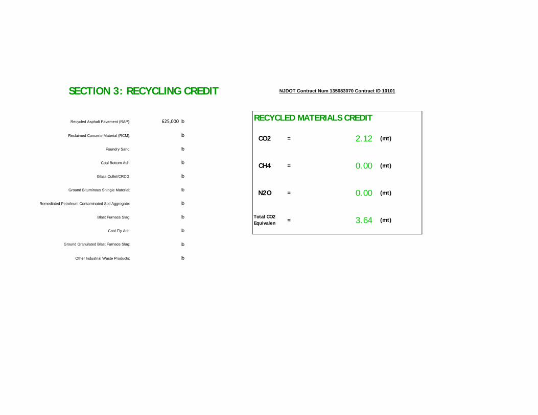
625,000 lb
lb
lb
lb
lb
lb
lb
lb
lb
lb
lb
Reclaimed Concrete Material (RCM): CO2 = 2.12 (mt)
SECTION 3: RECYCLING CREDIT NJDOT Contract Num 135083070 Contract ID 10101
RECYCLED MATERIALS CREDITRecycled Asphalt Pavement (RAP):
(mt)
Foundry Sand:
Coal Bottom Ash: CH4 = 0.00 (mt)
Glass Cullet/CRCG:
Ground Bituminous Shingle Material: N2O = 0.00
Ground Granulated Blast Furnace Slag:
Remediated Petroleum Contaminated Soil Aggregate:
Blast Furnace Slag: Total CO2 Equivalen = 3.64 (mt)
Other Industrial Waste Products:
Coal Fly Ash:
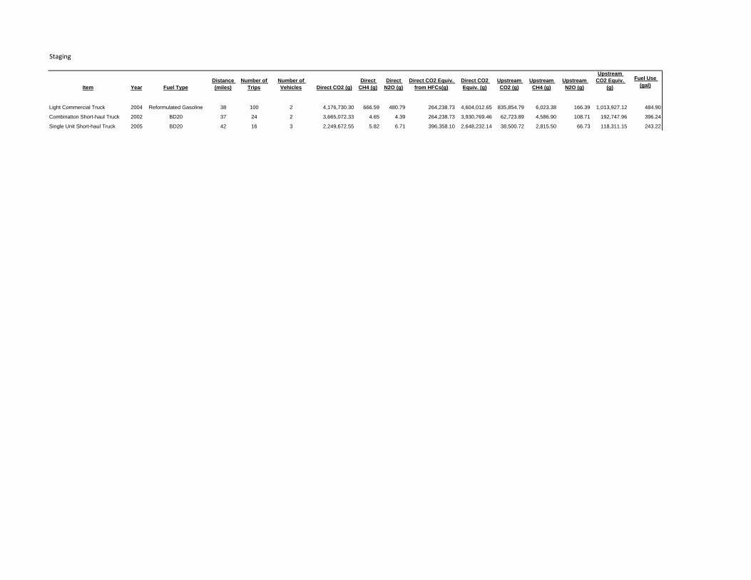
Staging
Item Year Fuel TypeDistance (miles)
Number of Trips
Number of Vehicles Direct CO2 (g)
Direct CH4 (g)
Direct N2O (g)
Direct CO2 Equiv. from HFCs(g)
Direct CO2 Equiv. (g)
Upstream CO2 (g)
Upstream CH4 (g)
Upstream N2O (g)
Upstream CO2 Equiv.
(g)
Fuel Use (gal)
Light Commercial Truck 2004 Reformulated Gasoline 38 100 2 4,176,730.30 666.59 480.79 264,238.73 4,604,012.65 835,854.79 6,023.38 166.39 1,013,927.12 484.90
Combination Short-haul Truck 2002 BD20 37 24 2 3,665,072.33 4.65 4.39 264,238.73 3,930,769.46 62,723.89 4,586.90 108.71 192,747.96 396.24
Single Unit Short-haul Truck 2005 BD20 42 16 3 2,249,672.55 5.82 6.71 396,358.10 2,648,232.14 38,500.72 2,815.50 66.73 118,311.15 243.22
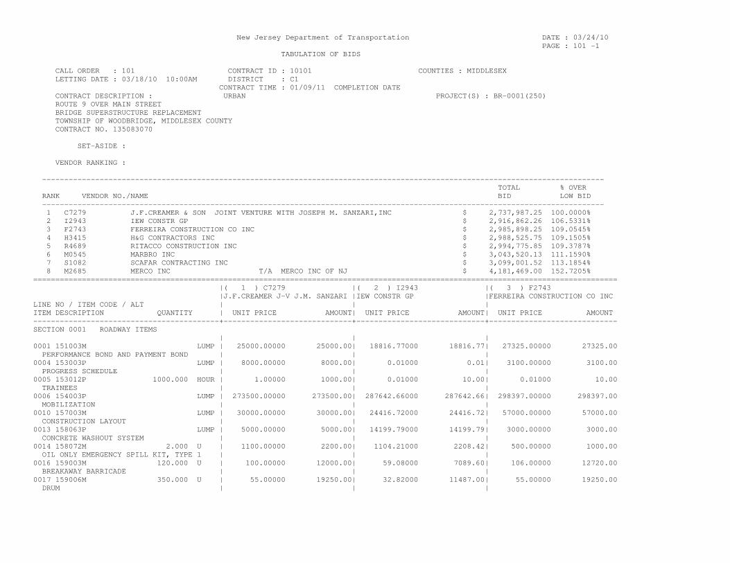
New Jersey Department of Transportation DATE : 03/24/10 PAGE : 101 -1 TABULATION OF BIDS CALL ORDER : 101 CONTRACT ID : 10101 COUNTIES : MIDDLESEX LETTING DATE : 03/18/10 10:00AM DISTRICT : C1 CONTRACT TIME : 01/09/11 COMPLETION DATE CONTRACT DESCRIPTION : URBAN PROJECT(S) : BR-0001(250) ROUTE 9 OVER MAIN STREET BRIDGE SUPERSTRUCTURE REPLACEMENT TOWNSHIP OF WOODBRIDGE, MIDDLESEX COUNTY CONTRACT NO. 135083070 SET-ASIDE : VENDOR RANKING : ------------------------------------------------------------------------------------------------------------------------------- TOTAL % OVER RANK VENDOR NO./NAME BID LOW BID ------------------------------------------------------------------------------------------------------------------------------- 1 C7279 J.F.CREAMER & SON JOINT VENTURE WITH JOSEPH M. SANZARI,INC $ 2,737,987.25 100.0000% 2 I2943 IEW CONSTR GP $ 2,916,862.26 106.5331% 3 F2743 FERREIRA CONSTRUCTION CO INC $ 2,985,898.25 109.0545% 4 H3415 H&G CONTRACTORS INC $ 2,988,525.75 109.1505% 5 R4689 RITACCO CONSTRUCTION INC $ 2,994,775.85 109.3787% 6 M0545 MARBRO INC $ 3,043,520.13 111.1590% 7 S1082 SCAFAR CONTRACTING INC $ 3,099,001.52 113.1854% 8 M2685 MERCO INC T/A MERCO INC OF NJ $ 4,181,469.00 152.7205% ==================================================================================================================================== |( 1 ) C7279 |( 2 ) I2943 |( 3 ) F2743 |J.F.CREAMER J-V J.M. SANZARI |IEW CONSTR GP |FERREIRA CONSTRUCTION CO INC LINE NO / ITEM CODE / ALT | | | ITEM DESCRIPTION QUANTITY | UNIT PRICE AMOUNT| UNIT PRICE AMOUNT| UNIT PRICE AMOUNT ------------------------------------------+-----------------------------+-----------------------------+----------------------------- SECTION 0001 ROADWAY ITEMS | | | 0001 151003M LUMP | 25000.00000 25000.00| 18816.77000 18816.77| 27325.00000 27325.00 PERFORMANCE BOND AND PAYMENT BOND | | | 0004 153003P LUMP | 8000.00000 8000.00| 0.01000 0.01| 3100.00000 3100.00 PROGRESS SCHEDULE | | | 0005 153012P 1000.000 HOUR | 1.00000 1000.00| 0.01000 10.00| 0.01000 10.00 TRAINEES | | | 0006 154003P LUMP | 273500.00000 273500.00| 287642.66000 287642.66| 298397.00000 298397.00 MOBILIZATION | | | 0010 157003M LUMP | 30000.00000 30000.00| 24416.72000 24416.72| 57000.00000 57000.00 CONSTRUCTION LAYOUT | | | 0013 158063P LUMP | 5000.00000 5000.00| 14199.79000 14199.79| 3000.00000 3000.00 CONCRETE WASHOUT SYSTEM | | | 0014 158072M 2.000 U | 1100.00000 2200.00| 1104.21000 2208.42| 500.00000 1000.00 OIL ONLY EMERGENCY SPILL KIT, TYPE 1 | | | 0016 159003M 120.000 U | 100.00000 12000.00| 59.08000 7089.60| 106.00000 12720.00 BREAKAWAY BARRICADE | | | 0017 159006M 350.000 U | 55.00000 19250.00| 32.82000 11487.00| 55.00000 19250.00 DRUM | | |

New Jersey Department of Transportation DATE : 03/24/10 PAGE : 101 -2 TABULATION OF BIDS CALL ORDER : 101 CONTRACT ID : 10101 COUNTIES : MIDDLESEX LETTING DATE : 03/18/10 10:00AM DISTRICT : C1 SET-ASIDE : ==================================================================================================================================== |( 1 ) C7279 |( 2 ) I2943 |( 3 ) F2743 |J.F.CREAMER J-V J.M. SANZARI |IEW CONSTR GP |FERREIRA CONSTRUCTION CO INC LINE NO / ITEM CODE / ALT | | | ITEM DESCRIPTION QUANTITY | UNIT PRICE AMOUNT| UNIT PRICE AMOUNT| UNIT PRICE AMOUNT ------------------------------------------+-----------------------------+-----------------------------+----------------------------- 0018 159009M 400.000 U | 12.00000 4800.00| 3.92000 1568.00| 6.00000 2400.00 TRAFFIC CONE | | | 0019 159012M 3550.000 SF | 8.50000 30175.00| 7.81000 27725.50| 19.00000 67450.00 CONSTRUCTION SIGNS | | | 0020 159015M 4.000 U | 1100.00000 4400.00| 697.10000 2788.40| 702.00000 2808.00 CONSTRUCTION IDENTIFICATION SIGN, 4' X | | | 8' | | | 0021 159021P 1450.000 LF | 74.00000 107300.00| 124.41000 180394.50| 37.00000 53650.00 CONSTRUCTION BARRIER CURB | | | 0022 159027M 6.000 U | 2100.00000 12600.00| 0.01000 0.06| 506.00000 3036.00 FLASHING ARROW BOARD, 4' X 8' | | | 0023 159030M 8.000 U | 8000.00000 64000.00| 749.62000 5996.96| 4045.00000 32360.00 PORTABLE VARIABLE MESSAGE SIGN | | | 0024 159108M 2.000 U | 11000.00000 22000.00| 0.01000 0.02| 5618.00000 11236.00 TRAFFIC CONTROL TRUCK WITH MOUNTED | | | CRASH CUSHION | | | 0025 159120M 2500.000 LF | 1.80000 4500.00| 1.51000 3775.00| 3.00000 7500.00 TEMPORARY PAVEMENT MARKING TAPE, 4" | | | 0026 159138M 40.000 T | 150.00000 6000.00| 223.07000 8922.80| 500.00000 20000.00 HMA PATCH | | | 0027 159141M 500.000 HOUR | 1.00000 500.00| 82.84000 41420.00| 58.00000 29000.00 TRAFFIC DIRECTOR, FLAGGER | | | 0028 160003M LUMP | 500.00000 500.00| 500.00000 500.00| 500.00000 500.00 FUEL PRICE ADJUSTMENT | | | 0029 161003P LUMP | 3000.00000 3000.00| 15282.47000 15282.47| 12000.00000 12000.00 FINAL CLEANUP | | | 0030 201003P LUMP | 40000.00000 40000.00| 39500.00000 39500.00| 30000.00000 30000.00 CLEARING SITE | | | 0031 202006M 10.000 CY | 300.00000 3000.00| 187.40000 1874.00| 251.00000 2510.00 EXCAVATION, TEST PIT | | | 0032 202009P 357.000 CY | 125.00000 44625.00| 20.84000 7439.88| 60.00000 21420.00 EXCAVATION, UNCLASSIFIED | | | 0033 202018P 20.000 CY | 25.00000 500.00| 51.72000 1034.40| 77.00000 1540.00 EXCAVATION, ACID PRODUCING SOIL | | | 0034 202021P 3178.000 SY | 12.00000 38136.00| 4.18000 13284.04| 5.00000 15890.00 REMOVAL OF PAVEMENT | | | 0035 202033M 2.000 U | 50.00000 100.00| 892.29000 1784.58| 524.00000 1048.00 SOIL SAMPLING AND ANALYSES, ACID | | | PRODUCING SOIL | | |
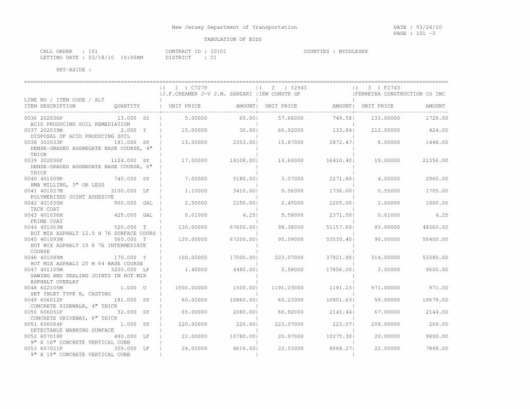
New Jersey Department of Transportation DATE : 03/24/10 PAGE : 101 -3 TABULATION OF BIDS CALL ORDER : 101 CONTRACT ID : 10101 COUNTIES : MIDDLESEX LETTING DATE : 03/18/10 10:00AM DISTRICT : C1 SET-ASIDE : ==================================================================================================================================== |( 1 ) C7279 |( 2 ) I2943 |( 3 ) F2743 |J.F.CREAMER J-V J.M. SANZARI |IEW CONSTR GP |FERREIRA CONSTRUCTION CO INC LINE NO / ITEM CODE / ALT | | | ITEM DESCRIPTION QUANTITY | UNIT PRICE AMOUNT| UNIT PRICE AMOUNT| UNIT PRICE AMOUNT ------------------------------------------+-----------------------------+-----------------------------+----------------------------- 0036 202036P 13.000 SY | 5.00000 65.00| 57.66000 749.58| 133.00000 1729.00 ACID PRODUCING SOIL REMEDIATION | | | 0037 202039M 2.000 T | 15.00000 30.00| 66.92000 133.84| 212.00000 424.00 DISPOSAL OF ACID PRODUCING SOIL | | | 0038 302033P 181.000 SY | 13.00000 2353.00| 15.87000 2872.47| 8.00000 1448.00 DENSE-GRADED AGGREGATE BASE COURSE, 4" | | | THICK | | | 0039 302036P 1124.000 SY | 17.00000 19108.00| 14.60000 16410.40| 19.00000 21356.00 DENSE-GRADED AGGREGATE BASE COURSE, 6" | | | THICK | | | 0040 401009P 740.000 SY | 7.00000 5180.00| 3.07000 2271.80| 4.00000 2960.00 HMA MILLING, 3" OR LESS | | | 0041 401027M 3100.000 LF | 1.10000 3410.00| 0.56000 1736.00| 0.55000 1705.00 POLYMERIZED JOINT ADHESIVE | | | 0042 401030M 900.000 GAL | 2.50000 2250.00| 2.45000 2205.00| 2.00000 1800.00 TACK COAT | | | 0043 401036M 425.000 GAL | 0.01000 4.25| 5.58000 2371.50| 0.01000 4.25 PRIME COAT | | | 0044 401063M 520.000 T | 130.00000 67600.00| 98.38000 51157.60| 93.00000 48360.00 HOT MIX ASPHALT 12.5 H 76 SURFACE COURS | | | 0045 401093M 560.000 T | 120.00000 67200.00| 95.59000 53530.40| 90.00000 50400.00 HOT MIX ASPHALT 19 H 76 INTERMEDIATE | | | COURSE | | | 0046 401099M 170.000 T | 100.00000 17000.00| 223.07000 37921.90| 314.00000 53380.00 HOT MIX ASPHALT 25 M 64 BASE COURSE | | | 0047 401105M 3200.000 LF | 1.40000 4480.00| 5.58000 17856.00| 3.00000 9600.00 SAWING AND SEALING JOINTS IN HOT MIX | | | ASPHALT OVERLAY | | | 0048 602105M 1.000 U | 1500.00000 1500.00| 1191.23000 1191.23| 971.00000 971.00 SET INLET TYPE B, CASTING | | | 0049 606012P 181.000 SY | 60.00000 10860.00| 60.23000 10901.63| 59.00000 10679.00 CONCRETE SIDEWALK, 4" THICK | | | 0050 606051P 32.000 SY | 65.00000 2080.00| 66.92000 2141.44| 67.00000 2144.00 CONCRETE DRIVEWAY, 6" THICK | | | 0051 606084P 1.000 SY | 220.00000 220.00| 223.07000 223.07| 209.00000 209.00 DETECTABLE WARNING SURFACE | | | 0052 607018P 490.000 LF | 22.00000 10780.00| 20.97000 10275.30| 20.00000 9800.00 9" X 16" CONCRETE VERTICAL CURB | | | 0053 607021P 359.000 LF | 24.00000 8616.00| 22.53000 8088.27| 22.00000 7898.00 9" X 18" CONCRETE VERTICAL CURB | | |

New Jersey Department of Transportation DATE : 03/24/10 PAGE : 101 -4 TABULATION OF BIDS CALL ORDER : 101 CONTRACT ID : 10101 COUNTIES : MIDDLESEX LETTING DATE : 03/18/10 10:00AM DISTRICT : C1 SET-ASIDE : ==================================================================================================================================== |( 1 ) C7279 |( 2 ) I2943 |( 3 ) F2743 |J.F.CREAMER J-V J.M. SANZARI |IEW CONSTR GP |FERREIRA CONSTRUCTION CO INC LINE NO / ITEM CODE / ALT | | | ITEM DESCRIPTION QUANTITY | UNIT PRICE AMOUNT| UNIT PRICE AMOUNT| UNIT PRICE AMOUNT ------------------------------------------+-----------------------------+-----------------------------+----------------------------- 0054 608003P 513.000 SY | 26.00000 13338.00| 30.32000 15554.16| 37.00000 18981.00 NONVEGETATIVE SURFACE, HOT MIX ASPHALT | | | 0055 609003M 1940.000 LF | 20.00000 38800.00| 24.39000 47316.60| 17.00000 32980.00 BEAM GUIDE RAIL | | | 0056 609006M 471.000 LF | 35.00000 16485.00| 24.44000 11511.24| 29.00000 13659.00 BEAM GUIDE RAIL, DUAL-FACED | | | 0057 609021M 795.000 LF | 6.00000 4770.00| 8.59000 6829.05| 7.00000 5565.00 RUB RAIL | | | 0058 609033M 1.000 U | 1000.00000 1000.00| 1070.71000 1070.71| 1250.00000 1250.00 CONTROLLED RELEASE TERMINAL | | | 0059 610003M 2500.000 LF | 1.00000 2500.00| 0.78000 1950.00| 0.45000 1125.00 TRAFFIC STRIPES, LONG LIFE, EPOXY RESIN | | | 4" | | | 0060 610009M 90.000 SF | 5.00000 450.00| 16.73000 1505.70| 4.00000 360.00 TRAFFIC MARKINGS, THERMOPLASTIC | | | 0061 610012M 21.000 U | 50.00000 1050.00| 68.32000 1434.72| 27.00000 567.00 RPM, MONO-DIRECTIONAL, WHITE LENS | | | 0062 652417M 1.000 U | 5500.00000 5500.00| 15409.85000 15409.85| 5998.00000 5998.00 SANITARY SEWER SERVICE CONNECTION | | | 0086 159066M 1.000 U | 12000.00000 12000.00| 20411.15000 20411.15| 6030.00000 6030.00 TEMPORARY CRASH CUSHION, QUADGUARD 4 | | | BAYS X 24" WIDE | | | 0087 602210M 15.000 U | 325.00000 4875.00| 1528.96000 22934.40| 413.00000 6195.00 BICYCLE SAFE GRATE | | | SECTION TOTALS | $ 1,085,590.25| $ 1,087,126.59| $ 1,053,727.25 ------------------------------------------+-----------------------------+-----------------------------+----------------------------- SECTION 0002 CONSTRUCTION ENGINEERING ITEMS | | | 0007 155006M 1.000 U | 30000.00000 30000.00| 45802.34000 45802.34| 20000.00000 20000.00 FIELD OFFICE TYPE B SET UP | | | 0008 155024M 9.000 MO | 1500.00000 13500.00| 2007.65000 18068.85| 2200.00000 19800.00 FIELD OFFICE TYPE B MAINTENANCE | | | 0009 155039M LUMP | 3250.00000 3250.00| 3250.00000 3250.00| 3250.00000 3250.00 TELEPHONE SERVICE | | | SECTION TOTALS | $ 46,750.00| $ 67,121.19| $ 43,050.00 ------------------------------------------+-----------------------------+-----------------------------+----------------------------- SECTION 0003 NON-PARTICIPATING ITMES (ROADWAY) | | | 0002 152003P LUMP | 9500.00000 9500.00| 5668.83000 5668.83| 15300.00000 15300.00 OWNER'S AND CONTRACTOR'S PROTECTIVE | | | LIABILITY INSURANCE | | |

New Jersey Department of Transportation DATE : 03/24/10 PAGE : 101 -5 TABULATION OF BIDS CALL ORDER : 101 CONTRACT ID : 10101 COUNTIES : MIDDLESEX LETTING DATE : 03/18/10 10:00AM DISTRICT : C1 SET-ASIDE : ==================================================================================================================================== |( 1 ) C7279 |( 2 ) I2943 |( 3 ) F2743 |J.F.CREAMER J-V J.M. SANZARI |IEW CONSTR GP |FERREIRA CONSTRUCTION CO INC LINE NO / ITEM CODE / ALT | | | ITEM DESCRIPTION QUANTITY | UNIT PRICE AMOUNT| UNIT PRICE AMOUNT| UNIT PRICE AMOUNT ------------------------------------------+-----------------------------+-----------------------------+----------------------------- 0003 152009P LUMP | 1000.00000 1000.00| 0.01000 0.01| 1.00000 1.00 POLLUTION LIABILITY INSURANCE | | | SECTION TOTALS | $ 10,500.00| $ 5,668.84| $ 15,301.00 ------------------------------------------+-----------------------------+-----------------------------+----------------------------- SECTION 0004 EROSION CONTROL | | | 0011 158012M 407.000 LF | 8.00000 3256.00| 6.18000 2515.26| 5.00000 2035.00 HEAVY DUTY SILT FENCE, BLACK | | | 0012 158030M 15.000 U | 150.00000 2250.00| 90.35000 1355.25| 150.00000 2250.00 INLET FILTER TYPE 2, 2' X 4' | | | 0015 158084M 26.000 CY | 75.00000 1950.00| 117.56000 3056.56| 150.00000 3900.00 EROSION CONTROL SEDIMENT REMOVAL | | | 0088 602214M 15.000 U | 200.00000 3000.00| 298.94000 4484.10| 270.00000 4050.00 INLET FACE PLATE | | | SECTION TOTALS | $ 10,456.00| $ 11,411.17| $ 12,235.00 ------------------------------------------+-----------------------------+-----------------------------+----------------------------- SECTION 0005 GENERAL LANDSCAPE ITEMS | | | 0063 804006P 301.000 SY | 2.50000 752.50| 5.58000 1679.58| 4.00000 1204.00 TOPSOILING, 4" THICK | | | 0064 806006P 301.000 SY | 1.50000 451.50| 0.84000 252.84| 2.00000 602.00 FERTILIZING AND SEEDING, TYPE A-3 | | | 0065 806018P 30.000 SY | 1.50000 45.00| 1.12000 33.60| 0.60000 18.00 FERTILIZING AND SEEDING, TYPE F | | | 0066 807003M 147.000 SY | 5.00000 735.00| 5.02000 737.94| 4.00000 588.00 TOPSOIL STABILIZATION, TYPE 1 MAT | | | 0067 809003M 198.000 SY | 1.50000 297.00| 0.84000 166.32| 1.50000 297.00 STRAW MULCHING | | | SECTION TOTALS | $ 2,281.00| $ 2,870.28| $ 2,709.00 ------------------------------------------+-----------------------------+-----------------------------+----------------------------- SECTION 0006 ROUTE 9 BRIDGE (STRUCTURE NO. 1210-150) | | | 0068 201006P LUMP | 180000.00000 180000.00| 179500.00000 179500.00| 166000.00000 166000.00 CLEARING SITE, BRIDGE (___) STR. NO. | | | 1210-150 | | | 0069 202009P 450.000 CY | 125.00000 56250.00| 73.56000 33102.00| 57.00000 25650.00 EXCAVATION, UNCLASSIFIED | | | 0070 504006P 24700.000 LB | 2.00000 49400.00| 3.92000 96824.00| 2.00000 49400.00 REINFORCEMENT STEEL, EPOXY-COATED | | |

New Jersey Department of Transportation DATE : 03/24/10 PAGE : 101 -6 TABULATION OF BIDS CALL ORDER : 101 CONTRACT ID : 10101 COUNTIES : MIDDLESEX LETTING DATE : 03/18/10 10:00AM DISTRICT : C1 SET-ASIDE : ==================================================================================================================================== |( 1 ) C7279 |( 2 ) I2943 |( 3 ) F2743 |J.F.CREAMER J-V J.M. SANZARI |IEW CONSTR GP |FERREIRA CONSTRUCTION CO INC LINE NO / ITEM CODE / ALT | | | ITEM DESCRIPTION QUANTITY | UNIT PRICE AMOUNT| UNIT PRICE AMOUNT| UNIT PRICE AMOUNT ------------------------------------------+-----------------------------+-----------------------------+----------------------------- 0071 504015P 115.000 CY | 600.00000 69000.00| 536.02000 61642.30| 323.00000 37145.00 CONCRETE FOOTING | | | 0072 504018P 15.000 CY | 1800.00000 27000.00| 2477.83000 37167.45| 1550.00000 23250.00 CONCRETE WING WALL | | | 0073 504024P 290.000 CY | 600.00000 174000.00| 598.89000 173678.10| 800.00000 232000.00 CONCRETE ABUTMENT WALL | | | 0074 504036P 70.000 SY | 50.00000 3500.00| 62.27000 4358.90| 59.00000 4130.00 EPOXY WATERPROOFING | | | 0075 504061P LUMP | 1500.00000 1500.00| 41271.43000 41271.43| 50000.00000 50000.00 TEMPORARY SHORING | | | 0076 505063P 5420.000 SF | 151.00000 818420.00| 154.79000 838961.80| 182.00000 986440.00 PREFABRICATED SUPERSTRUCTURE UNITS | | | 0077 507020P 125.000 LF | 140.00000 17500.00| 131.37000 16421.25| 210.00000 26250.00 ASPHALTIC BRIDGE JOINT SYSTEM | | | 0078 507027M 2.000 U | 1200.00000 2400.00| 767.12000 1534.24| 1200.00000 2400.00 DATE PANEL | | | 0079 507033P 25.000 CY | 450.00000 11250.00| 0.01000 0.25| 780.00000 19500.00 CONCRETE BRIDGE SIDEWALK, HPC | | | 0080 507039P 292.000 LF | 250.00000 73000.00| 256.53000 74906.76| 240.00000 70080.00 CONCRETE BRIDGE PARAPET, HPC | | | 0081 507047M 172.000 LF | 220.00000 37840.00| 503.70000 86636.40| 391.00000 67252.00 21" BY 36" CONCRETE BARRIER CURB, | | | BRIDGE, PRECAST | | | 0082 551021M 162.000 LF | 160.00000 25920.00| 219.29000 35524.98| 295.00000 47790.00 HEADER RECONSTRUCTION | | | 0083 555006M 55.000 T | 210.00000 11550.00| 446.15000 24538.25| 419.00000 23045.00 BRIDGE DECK WATERPROOF SURFACE COURSE | | | 0084 609004M 160.000 LF | 120.00000 19200.00| 125.20000 20032.00| 116.00000 18560.00 BEAM GUIDE RAIL, BRIDGE | | | 0085 701021P 312.000 LF | 15.00000 4680.00| 53.09000 16564.08| 32.00000 9984.00 3" RIGID METALLIC CONDUIT | | | SECTION TOTALS | $ 1,582,410.00| $ 1,742,664.19| $ 1,858,876.00 ------------------------------------------+-----------------------------+-----------------------------+----------------------------- CONTRACT TOTALS | $ 2,737,987.25| $ 2,916,862.26| $ 2,985,898.25 ==================================================================================================================================== I CERTIFY THAT THE ABOVE IS AN EXACT TRANSCRIPT OF THE ORIGINAL BID PROPOSAL, EXCEPT THAT ERRORS, IF ANY, IN EXTENSION AND ADDITIONS HAVE BEEN CORRECTED. SIGNED,
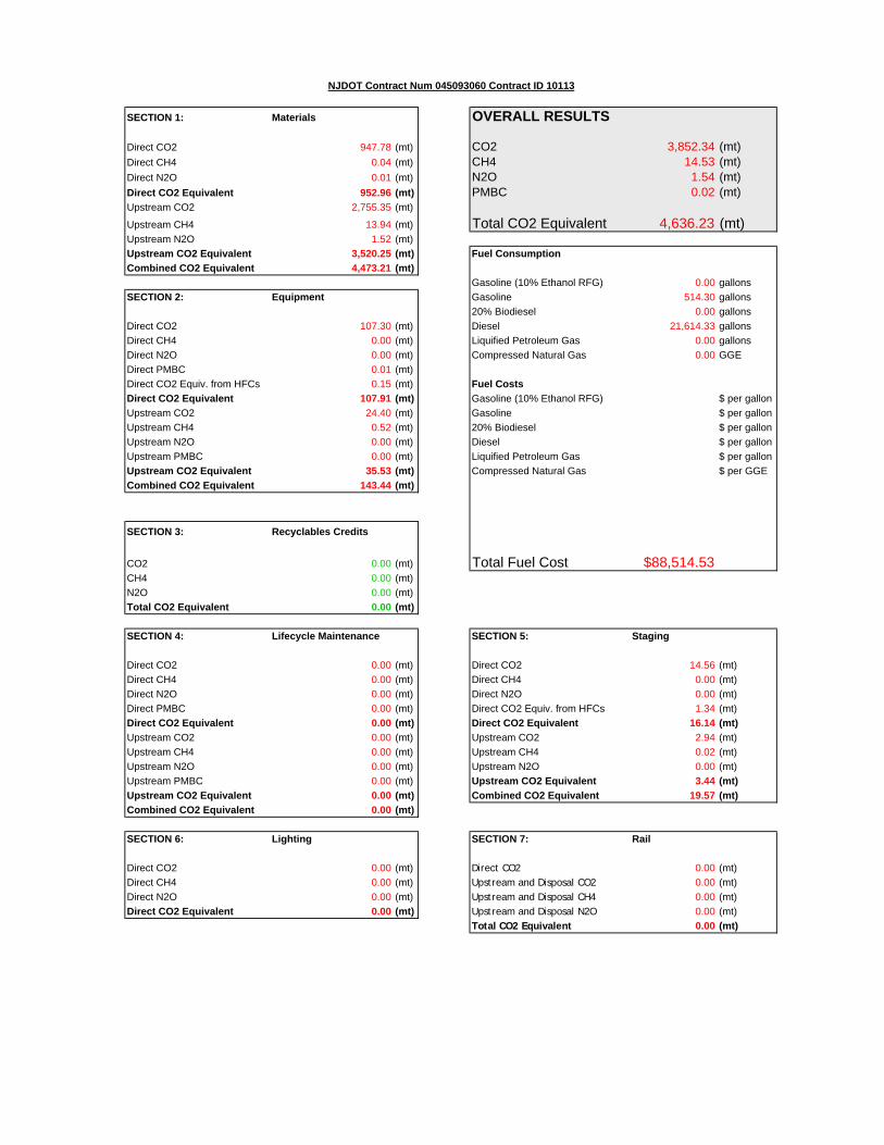
SECTION 1: Materials OVERALL RESULTS
Direct CO2 947.78 (mt) CO2 3,852.34 (mt)Direct CH4 0.04 (mt) CH4 14.53 (mt)Direct N2O 0.01 (mt) N2O 1.54 (mt)Direct CO2 Equivalent 952.96 (mt) PMBC 0.02 (mt)Upstream CO2 2,755.35 (mt)
Upstream CH4 13.94 (mt) Total CO2 Equivalent 4,636.23 (mt)Upstream N2O 1.52 (mt)Upstream CO2 Equivalent 3,520.25 (mt) Fuel ConsumptionCombined CO2 Equivalent 4,473.21 (mt)
Gasoline (10% Ethanol RFG) 0.00 gallonsSECTION 2: Equipment Gasoline 514.30 gallons
20% Biodiesel 0.00 gallonsDirect CO2 107.30 (mt) Diesel 21,614.33 gallonsDirect CH4 0.00 (mt) Liquified Petroleum Gas 0.00 gallonsDirect N2O 0.00 (mt) Compressed Natural Gas 0.00 GGEDirect PMBC 0.01 (mt)Direct CO2 Equiv. from HFCs 0.15 (mt) Fuel CostsDirect CO2 Equivalent 107.91 (mt) Gasoline (10% Ethanol RFG) $ per gallonUpstream CO2 24.40 (mt) Gasoline $ per gallonUpstream CH4 0.52 (mt) 20% Biodiesel $ per gallonUpstream N2O 0.00 (mt) Diesel $ per gallonUpstream PMBC 0.00 (mt) Liquified Petroleum Gas $ per gallonUpstream CO2 Equivalent 35.53 (mt) Compressed Natural Gas $ per GGECombined CO2 Equivalent 143.44 (mt)
SECTION 3: Recyclables Credits
CO2 0.00 (mt) Total Fuel Cost $88,514.53CH4 0.00 (mt)N2O 0.00 (mt)Total CO2 Equivalent 0.00 (mt)
SECTION 4: Lifecycle Maintenance SECTION 5: Staging
Direct CO2 0.00 (mt) Direct CO2 14.56 (mt)Direct CH4 0.00 (mt) Direct CH4 0.00 (mt)Direct N2O 0.00 (mt) Direct N2O 0.00 (mt)Direct PMBC 0.00 (mt) Direct CO2 Equiv. from HFCs 1.34 (mt)Direct CO2 Equivalent 0.00 (mt) Direct CO2 Equivalent 16.14 (mt)Upstream CO2 0.00 (mt) Upstream CO2 2.94 (mt)Upstream CH4 0.00 (mt) Upstream CH4 0.02 (mt)Upstream N2O 0.00 (mt) Upstream N2O 0.00 (mt)Upstream PMBC 0.00 (mt) Upstream CO2 Equivalent 3.44 (mt)Upstream CO2 Equivalent 0.00 (mt) Combined CO2 Equivalent 19.57 (mt)Combined CO2 Equivalent 0.00 (mt)
SECTION 6: Lighting SECTION 7: Rail
Direct CO2 0.00 (mt) Direct CO2 0.00 (mt)Direct CH4 0.00 (mt) Upstream and Disposal CO2 0.00 (mt)Direct N2O 0.00 (mt) Upstream and Disposal CH4 0.00 (mt)Direct CO2 Equivalent 0.00 (mt) Upstream and Disposal N2O 0.00 (mt)
Total CO2 Equivalent 0.00 (mt)
NJDOT Contract Num 045093060 Contract ID 10113

Materials
Item Code Description Value Unit Cement Ratio Aggregate Ratio Heating Temp. % Binder % Moisture Cutback Depth (feet)
612009P Guide Sign, Type Ga, Breakaway Supports 12.00 Sq. Feet N/A N/A N/A N/A N/A Non-Solvent-N/A N/A
607018P 9" X 16" Concrete Vertical Curb 1,308.00 Feet 0.15 0.80 N/A N/A N/A Non-Solvent-N/A N/A
606075P Concrete Island, 4" Thick 160.00 Sq. Yard 0.15 0.80 N/A N/A N/A Non-Solvent-N/A N/A
602214M Inlet Face Plate 134.00 Units N/A N/A N/A N/A N/A Non-Solvent-N/A N/A
602213M Curb Piece 25.00 Units N/A N/A N/A N/A N/A Non-Solvent-N/A 15.00
602210M Bicycle Safe Grate 35.00 Units N/A N/A N/A N/A N/A Non-Solvent-N/A N/A
602159M Reconstructed Inlet, Type E, Using New Casting 20.00 Units 0.15 0.80 N/A N/A N/A Non-Solvent-N/A 15.00
602153M Reconstructed Inlet, Type B, Using New Casting 60.00 Units 0.15 0.80 N/A N/A N/A Non-Solvent-N/A 15.00
602150M Reconstructed Inlet, Type A, Using New Casting 20.00 Units 0.15 0.80 N/A N/A N/A Non-Solvent-N/A 15.00
401066M HMA - Intermediate Course 11,190.00 Tons N/A N/A 325.00 0.07 0.04 Non-Solvent-N/A N/A
404003M Stone Matrix Asphalt 9.5mm Surface Course 22,388.00 Tons N/A N/A 325.00 0.05 0.04 Non-Solvent-N/A N/A
401099M HMA - Base Course 10,320.00 Tons N/A N/A 325.00 0.04 0.04 Non-Solvent-N/A N/A
401066M HMA - Intermediate Course 4,270.00 Tons N/A N/A 325.00 0.04 0.04 Non-Solvent-N/A N/A
401036M Prime Coat, Cut-Back Asphalt 5,441.00 Gallons N/A N/A 120.00 N/A N/A MC-0.3 N/A
401030M Tack Coat 15,217.00 Gallons N/A N/A 145.00 N/A N/A Non-Solvent-0 N/A
301006P Subbase 3,628.00 Cu. Yards N/A N/A N/A N/A N/A Non-Solvent-N/A N/A
Direct CO2 (g) Direct CH4 (g) Direct N2O (g) Direct CO2 Equiv. (g) Upstream CO2 (g) Upstream CH4 (g) Upstream N2O (g) Upstream CO2 Equiv. (g)
612009P Guide Sign, Type Ga, Breakaway Supports 0.00 0.00 0.00 0.00 144,254.19 213.40 1.30 149,137.46
607018P 9" X 16" Concrete Vertical Curb 0.00 0.00 0.00 0.00 23,140,447.01 1,401,738.34 1,383,781.13 481,549,103.46
606075P Concrete Island, 4" Thick 0.00 0.00 0.00 0.00 6,048,453.29 3,979.96 617.86 6,323,569.99
602214M Inlet Face Plate 0.00 0.00 0.00 0.00 48,719,458.63 35,925.93 164.45 49,524,883.95
602213M Curb Piece 0.00 0.00 0.00 0.00 4,670,579.56 3,444.10 15.77 4,747,793.12
602210M Bicycle Safe Grate 0.00 0.00 0.00 0.00 12,725,231.73 9,383.64 42.95 12,935,604.02
602159M Reconstructed Inlet, Type E, Using New Casting 0.00 0.00 0.00 0.00 125,609,886.00 111,364.57 4,585.31 129,369,987.45
602153M Reconstructed Inlet, Type B, Using New Casting 0.00 0.00 0.00 0.00 376,829,657.99 334,093.72 13,755.92 388,109,962.34
602150M Reconstructed Inlet, Type A, Using New Casting 0.00 0.00 0.00 0.00 102,602,051.18 90,550.02 3,495.27 105,587,136.43
401066M HMA - Intermediate Course 218,395,721.14 8,557.37 3,309.72 219,601,439.64 599,043,647.71 3,502,475.20 9,738.22 675,614,475.02
404003M Stone Matrix Asphalt 9.5mm Surface Course 435,241,192.52 17,096.11 6,595.92 437,644,945.22 908,166,953.48 5,375,786.16 14,791.17 1,025,643,725.47
401099M HMA - Base Course 200,039,381.74 7,872.08 3,031.51 201,144,463.90 318,250,165.18 1,913,927.15 5,195.95 360,053,380.73
401066M HMA - Intermediate Course 82,768,232.56 3,257.15 1,254.32 83,225,471.01 131,679,089.66 791,905.90 2,149.88 148,975,575.17
401036M Prime Coat, Cut-Back Asphalt 10,888,868.83 1.52 1.59 10,889,392.62 14,967,151.19 83,680.09 241.70 16,799,359.82
401030M Tack Coat 451,273.45 6.55 6.85 453,533.62 45,616,931.76 255,263.47 736.75 51,205,855.81
301006P Subbase 0.00 0.00 0.00 0.00 37,139,659.02 27,821.89 83,662.79 63,659,382.47
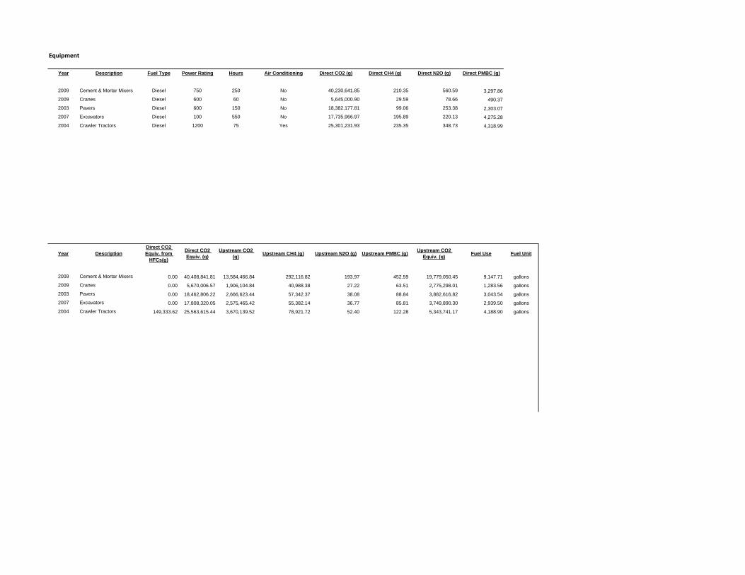
Equipment
Year Description Fuel Type Power Rating Hours Air Conditioning Direct CO2 (g) Direct CH4 (g) Direct N2O (g) Direct PMBC (g)
2009 Cement & Mortar Mixers Diesel 750 250 No 40,230,641.85 210.35 560.59 3,297.86
2009 Cranes Diesel 600 60 No 5,645,000.90 29.59 78.66 490.37
2003 Pavers Diesel 600 150 No 18,382,177.81 99.06 253.38 2,303.07
2007 Excavators Diesel 100 550 No 17,735,966.97 195.89 220.13 4,275.28
2004 Crawler Tractors Diesel 1200 75 Yes 25,301,231.93 235.35 348.73 4,318.99
Year DescriptionDirect CO2 Equiv. from
HFCs(g)
Direct CO2 Equiv. (g)
Upstream CO2 (g) Upstream CH4 (g) Upstream N2O (g) Upstream PMBC (g) Upstream CO2
Equiv. (g) Fuel Use Fuel Unit
2009 Cement & Mortar Mixers 0.00 40,408,841.81 13,584,466.84 292,116.82 193.97 452.59 19,779,050.45 9,147.71 gallons
2009 Cranes 0.00 5,670,006.57 1,906,104.84 40,988.38 27.22 63.51 2,775,298.01 1,283.56 gallons
2003 Pavers 0.00 18,462,806.22 2,666,623.44 57,342.37 38.08 88.84 3,882,616.82 3,043.54 gallons
2007 Excavators 0.00 17,808,320.05 2,575,465.42 55,382.14 36.77 85.81 3,749,890.30 2,939.50 gallons
2004 Crawler Tractors 149,333.62 25,563,615.44 3,670,139.52 78,921.72 52.40 122.28 5,343,741.17 4,188.90 gallons

Staging
Item Year Fuel TypeDistance (miles)
Number of Trips
Number of Vehicles Direct CO2 (g)
Direct CH4 (g)
Direct N2O (g)
Direct CO2 Equiv. from
HFCs(g)Direct CO2 Equiv. (g)
Upstream CO2 (g)
Upstream CH4 (g)
Upstream N2O (g)
Upstream CO2 Equiv. (g)
Fuel Use (gal)
Combination Short-haul Truck 2008 Diesel Fuel 60 16 3 5,948,342.23 34.35 7.21 448,000.85 6,399,300.58 1,208,450.66 8,158.01 20.98 1,386,273.34 593.74
Single Unit Short-haul Truck 2003 Diesel Fuel 25 50 3 4,181,610.60 11.48 12.38 448,000.85 4,633,690.95 849,525.89 5,734.98 14.75 974,533.04 417.39
Light Commercial Truck 2000 Reformulated Gasoline 34 80 3 4,429,997.82 876.41 675.32 448,000.85 5,105,754.02 886,538.22 6,388.61 176.48 1,075,408.26 514.30

New Jersey Department of Transportation DATE : 02/08/11 PAGE : 113 -1 TABULATION OF BIDS CALL ORDER : 113 CONTRACT ID : 10113 COUNTIES : HUDSON LETTING DATE : 02/08/11 10:00AM DISTRICT : CONTRACT TIME : 01/21/12 COMPLETION DATE CONTRACT DESCRIPTION : URBAN PROJECT(S) : NHS-0033(280) ROUTE 1&9 NORTH AVENUE TO HAYNES AVENUE RESURFACING (M.P. 45.5 TO 47.6) CONTRACT NO. 045093060,MILL AND PAVE CITY OF NEWARK, CITY OF ELIZABETH,COUNTY OF ESSEX, COUNTY OF UNION SET-ASIDE : VENDOR RANKING : ------------------------------------------------------------------------------------------------------------------------------- TOTAL % OVER RANK VENDOR NO./NAME BID LOW BID ------------------------------------------------------------------------------------------------------------------------------- 1 D2395 DELLA PELLO PAVING INC $ 6,375,750.69 100.0000% 2 T4306 TILCON NEW YORK INC $ 6,588,000.00 103.3290% 3 I5980 INTERCOUNTY PAVING ASSOC LLC $ 6,993,888.23 109.6951% 4 S0503 JOSEPH M SANZARI INC $ 7,144,273.21 112.0538% 5 S1389 SCHIFANO CONSTRUCTION CORP $ 7,195,394.22 112.8556% 6 S8162 .STAVOLA CONTRACTING CO., INC. $ 7,294,770.88 114.4143% 7 C7444 CRISDEL GROUP, INC $ 7,676,785.00 120.4060% 8 N2943 NEW PRINCE CONCRETE CONSTRUCTION CO $ 8,400,236.16 131.7529% ==================================================================================================================================== |( 1 ) D2395 |( 2 ) T4306 |( 3 ) I5980 |DELLA PELLO PAVING INC |TILCON NEW YORK INC |INTERCOUNTY PAVING ASSOC LLC LINE NO / ITEM CODE / ALT | | | ITEM DESCRIPTION QUANTITY | UNIT PRICE AMOUNT| UNIT PRICE AMOUNT| UNIT PRICE AMOUNT ------------------------------------------+-----------------------------+-----------------------------+----------------------------- SECTION 0001 ROADWAY | | | 0001 151003M LUMP | 31645.00000 31645.00| 19620.76000 19620.76| 37500.00000 37500.00 PERFORMANCE BOND AND PAYMENT BOND | | | 0004 153003P LUMP | 3500.00000 3500.00| 1000.00000 1000.00| 11500.00000 11500.00 PROGRESS SCHEDULE | | | 0005 153006P 4.000 U | 632.50000 2530.00| 600.00000 2400.00| 630.00000 2520.00 PROGRESS SCHEDULE UPDATE | | | 0006 153012P 740.000 HOUR | 3.00000 2220.00| 1.00000 740.00| 0.01000 7.40 TRAINEES | | | 0007 154003P LUMP | 323845.00000 323845.00| 496507.00000 496507.00| 499811.97000 499811.97 MOBILIZATION | | | 0011 157003M LUMP | 10000.00000 10000.00| 1.00000 1.00| 7250.00000 7250.00 CONSTRUCTION LAYOUT | | | 0018 159003M 100.000 U | 1.00000 100.00| 1.00000 100.00| 115.00000 11500.00 BREAKAWAY BARRICADE | | | 0019 159006M 250.000 U | 1.00000 250.00| 1.00000 250.00| 1.00000 250.00 DRUM | | |
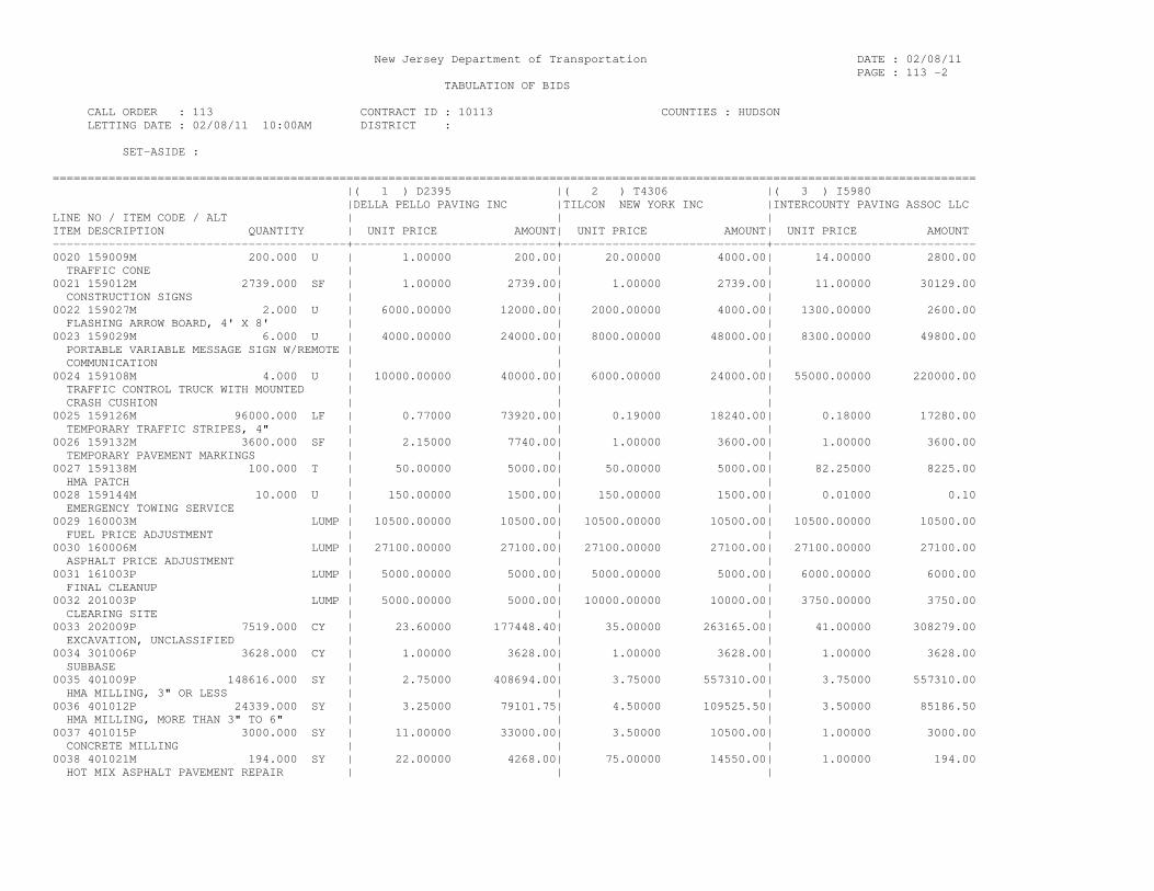
New Jersey Department of Transportation DATE : 02/08/11 PAGE : 113 -2 TABULATION OF BIDS CALL ORDER : 113 CONTRACT ID : 10113 COUNTIES : HUDSON LETTING DATE : 02/08/11 10:00AM DISTRICT : SET-ASIDE : ==================================================================================================================================== |( 1 ) D2395 |( 2 ) T4306 |( 3 ) I5980 |DELLA PELLO PAVING INC |TILCON NEW YORK INC |INTERCOUNTY PAVING ASSOC LLC LINE NO / ITEM CODE / ALT | | | ITEM DESCRIPTION QUANTITY | UNIT PRICE AMOUNT| UNIT PRICE AMOUNT| UNIT PRICE AMOUNT ------------------------------------------+-----------------------------+-----------------------------+----------------------------- 0020 159009M 200.000 U | 1.00000 200.00| 20.00000 4000.00| 14.00000 2800.00 TRAFFIC CONE | | | 0021 159012M 2739.000 SF | 1.00000 2739.00| 1.00000 2739.00| 11.00000 30129.00 CONSTRUCTION SIGNS | | | 0022 159027M 2.000 U | 6000.00000 12000.00| 2000.00000 4000.00| 1300.00000 2600.00 FLASHING ARROW BOARD, 4' X 8' | | | 0023 159029M 6.000 U | 4000.00000 24000.00| 8000.00000 48000.00| 8300.00000 49800.00 PORTABLE VARIABLE MESSAGE SIGN W/REMOTE | | | COMMUNICATION | | | 0024 159108M 4.000 U | 10000.00000 40000.00| 6000.00000 24000.00| 55000.00000 220000.00 TRAFFIC CONTROL TRUCK WITH MOUNTED | | | CRASH CUSHION | | | 0025 159126M 96000.000 LF | 0.77000 73920.00| 0.19000 18240.00| 0.18000 17280.00 TEMPORARY TRAFFIC STRIPES, 4" | | | 0026 159132M 3600.000 SF | 2.15000 7740.00| 1.00000 3600.00| 1.00000 3600.00 TEMPORARY PAVEMENT MARKINGS | | | 0027 159138M 100.000 T | 50.00000 5000.00| 50.00000 5000.00| 82.25000 8225.00 HMA PATCH | | | 0028 159144M 10.000 U | 150.00000 1500.00| 150.00000 1500.00| 0.01000 0.10 EMERGENCY TOWING SERVICE | | | 0029 160003M LUMP | 10500.00000 10500.00| 10500.00000 10500.00| 10500.00000 10500.00 FUEL PRICE ADJUSTMENT | | | 0030 160006M LUMP | 27100.00000 27100.00| 27100.00000 27100.00| 27100.00000 27100.00 ASPHALT PRICE ADJUSTMENT | | | 0031 161003P LUMP | 5000.00000 5000.00| 5000.00000 5000.00| 6000.00000 6000.00 FINAL CLEANUP | | | 0032 201003P LUMP | 5000.00000 5000.00| 10000.00000 10000.00| 3750.00000 3750.00 CLEARING SITE | | | 0033 202009P 7519.000 CY | 23.60000 177448.40| 35.00000 263165.00| 41.00000 308279.00 EXCAVATION, UNCLASSIFIED | | | 0034 301006P 3628.000 CY | 1.00000 3628.00| 1.00000 3628.00| 1.00000 3628.00 SUBBASE | | | 0035 401009P 148616.000 SY | 2.75000 408694.00| 3.75000 557310.00| 3.75000 557310.00 HMA MILLING, 3" OR LESS | | | 0036 401012P 24339.000 SY | 3.25000 79101.75| 4.50000 109525.50| 3.50000 85186.50 HMA MILLING, MORE THAN 3" TO 6" | | | 0037 401015P 3000.000 SY | 11.00000 33000.00| 3.50000 10500.00| 1.00000 3000.00 CONCRETE MILLING | | | 0038 401021M 194.000 SY | 22.00000 4268.00| 75.00000 14550.00| 1.00000 194.00 HOT MIX ASPHALT PAVEMENT REPAIR | | |

New Jersey Department of Transportation DATE : 02/08/11 PAGE : 113 -3 TABULATION OF BIDS CALL ORDER : 113 CONTRACT ID : 10113 COUNTIES : HUDSON LETTING DATE : 02/08/11 10:00AM DISTRICT : SET-ASIDE : ==================================================================================================================================== |( 1 ) D2395 |( 2 ) T4306 |( 3 ) I5980 |DELLA PELLO PAVING INC |TILCON NEW YORK INC |INTERCOUNTY PAVING ASSOC LLC LINE NO / ITEM CODE / ALT | | | ITEM DESCRIPTION QUANTITY | UNIT PRICE AMOUNT| UNIT PRICE AMOUNT| UNIT PRICE AMOUNT ------------------------------------------+-----------------------------+-----------------------------+----------------------------- 0039 401030M 15217.000 GAL | 0.01000 152.17| 0.01000 152.17| 2.50000 38042.50 TACK COAT | | | 0040 401036M 5441.000 GAL | 0.01000 54.41| 0.01000 54.41| 0.01000 54.41 PRIME COAT | | | 0041 401066M 4270.000 T | 58.80000 251076.00| 75.00000 320250.00| 63.00000 269010.00 HOT MIX ASPHALT 9.5 M 64 INTERMEDIATE | | | COURSE | | | 0042 401099M 10320.000 T | 60.70000 626424.00| 65.00000 670800.00| 68.00000 701760.00 HOT MIX ASPHALT 25 M 64 BASE COURSE | | | 0043 401108M 108.000 U | 80.00000 8640.00| 25.00000 2700.00| 60.00000 6480.00 CORE SAMPLES, HOT MIX ASPHALT | | | 0044 404003M 22388.000 T | 97.60000 2185068.80| 92.25000 2065293.00| 100.00000 2238800.00 STONE MATRIX ASPHALT 9.5 MM SURFACE | | | COURSE | | | 0045 409003P 11190.000 T | 108.85000 1218031.50| 100.00000 1119000.00| 113.75000 1272862.50 BINDER RICH INTERMEDIATE COURSE, 4.75MM | | | 0046 453006M 722.000 SY | 225.00000 162450.00| 175.00000 126350.00| 150.00000 108300.00 FULL DEPTH CONCRETE PAVEMENT REPAIR, HM | | | 0049 602099M 50.000 U | 600.00000 30000.00| 247.74000 12387.00| 575.00000 28750.00 RESET EXISTING CASTING | | | 0050 602150M 20.000 U | 1400.00000 28000.00| 1728.96000 34579.20| 700.00000 14000.00 RECONSTRUCTED INLET, TYPE A, USING NEW | | | CASTING | | | 0051 602153M 60.000 U | 1500.00000 90000.00| 1335.47000 80128.20| 700.00000 42000.00 RECONSTRUCTED INLET, TYPE B, USING NEW | | | CASTING | | | 0052 602159M 20.000 U | 1575.00000 31500.00| 2075.46000 41509.20| 700.00000 14000.00 RECONSTRUCTED INLET, TYPE E, USING NEW | | | CASTING | | | 0053 602210M 35.000 U | 245.00000 8575.00| 353.49000 12372.15| 300.00000 10500.00 BICYCLE SAFE GRATE | | | 0054 602213M 25.000 U | 285.00000 7125.00| 403.35000 10083.75| 325.00000 8125.00 CURB PIECE | | | 0055 602214M 134.000 U | 225.00000 30150.00| 418.34000 56057.56| 300.00000 40200.00 INLET FACE PLATE | | | 0057 606075P 160.000 SY | 66.00000 10560.00| 103.85000 16616.00| 93.00000 14880.00 CONCRETE ISLAND, 4" THICK | | | 0058 607018P 1308.000 LF | 80.00000 104640.00| 45.00000 58860.00| 46.00000 60168.00 9" X 16" CONCRETE VERTICAL CURB | | |
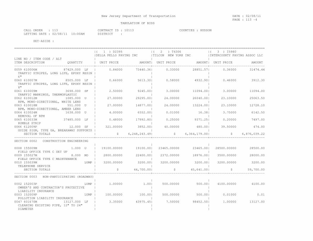
New Jersey Department of Transportation DATE : 02/08/11 PAGE : 113 -4 TABULATION OF BIDS CALL ORDER : 113 CONTRACT ID : 10113 COUNTIES : HUDSON LETTING DATE : 02/08/11 10:00AM DISTRICT : SET-ASIDE : ==================================================================================================================================== |( 1 ) D2395 |( 2 ) T4306 |( 3 ) I5980 |DELLA PELLO PAVING INC |TILCON NEW YORK INC |INTERCOUNTY PAVING ASSOC LLC LINE NO / ITEM CODE / ALT | | | ITEM DESCRIPTION QUANTITY | UNIT PRICE AMOUNT| UNIT PRICE AMOUNT| UNIT PRICE AMOUNT ------------------------------------------+-----------------------------+-----------------------------+----------------------------- 0059 610006M 87429.000 LF | 0.84000 73440.36| 0.33000 28851.57| 0.36000 31474.44 TRAFFIC STRIPES, LONG LIFE, EPOXY RESIN | | | 6" | | | 0060 610007M 8505.000 LF | 0.66000 5613.30| 0.58000 4932.90| 0.46000 3912.30 TRAFFIC STRIPES, LONG LIFE, EPOXY RESIN | | | 8" | | | 0061 610009M 3698.000 SF | 2.50000 9245.00| 3.00000 11094.00| 3.00000 11094.00 TRAFFIC MARKINGS, THERMOPLASTIC | | | 0062 610012M 1085.000 U | 27.00000 29295.00| 24.00000 26040.00| 23.10000 25063.50 RPM, MONO-DIRECTIONAL, WHITE LENS | | | 0063 610018M 551.000 U | 27.00000 14877.00| 24.00000 13224.00| 23.10000 12728.10 RPM, MONO-DIRECTIONAL, AMBER LENS | | | 0064 610024M 1638.000 U | 4.00000 6552.00| 0.01000 16.38| 3.75000 6142.50 REMOVAL OF RPM | | | 0065 610033M 37485.000 LF | 0.48000 17992.80| 0.25000 9371.25| 0.20000 7497.00 RUMBLE STRIP | | | 0066 612009P 12.000 SF | 321.00000 3852.00| 40.00000 480.00| 39.50000 474.00 GUIDE SIGN, TYPE GA, BREAKAWAY SUPPORTS | | | SECTION TOTALS | $ 6,248,243.49| $ 6,364,179.00| $ 6,876,039.22 ------------------------------------------+-----------------------------+-----------------------------+----------------------------- SECTION 0002 CONSTRUCTION ENGINEERING | | | 0008 155009M 1.000 U | 19100.00000 19100.00| 23465.00000 23465.00| 28500.00000 28500.00 FIELD OFFICE TYPE C SET UP | | | 0009 155027M 8.000 MO | 2800.00000 22400.00| 2372.00000 18976.00| 3500.00000 28000.00 FIELD OFFICE TYPE C MAINTENANCE | | | 0010 155039M LUMP | 3200.00000 3200.00| 3200.00000 3200.00| 3200.00000 3200.00 TELEPHONE SERVICE | | | SECTION TOTALS | $ 44,700.00| $ 45,641.00| $ 59,700.00 ------------------------------------------+-----------------------------+-----------------------------+----------------------------- SECTION 0003 NON-PARTICIPATING (ROADWAY) | | | 0002 152003P LUMP | 1.00000 1.00| 500.00000 500.00| 4100.00000 4100.00 OWNER'S AND CONTRACTOR'S PROTECTIVE | | | LIABILITY INSURANCE | | | 0003 152009P LUMP | 100.00000 100.00| 500.00000 500.00| 0.01000 0.01 POLLUTION LIABILITY INSURANCE | | | 0047 601670M 13127.000 LF | 3.35000 43975.45| 7.50000 98452.50| 1.00000 13127.00 CLEANING EXISTING PIPE, 12" TO 24" | | | DIAMETER | | |

New Jersey Department of Transportation DATE : 02/08/11 PAGE : 113 -5 TABULATION OF BIDS CALL ORDER : 113 CONTRACT ID : 10113 COUNTIES : HUDSON LETTING DATE : 02/08/11 10:00AM DISTRICT : SET-ASIDE : ==================================================================================================================================== |( 1 ) D2395 |( 2 ) T4306 |( 3 ) I5980 |DELLA PELLO PAVING INC |TILCON NEW YORK INC |INTERCOUNTY PAVING ASSOC LLC LINE NO / ITEM CODE / ALT | | | ITEM DESCRIPTION QUANTITY | UNIT PRICE AMOUNT| UNIT PRICE AMOUNT| UNIT PRICE AMOUNT ------------------------------------------+-----------------------------+-----------------------------+----------------------------- 0048 601672M 473.000 LF | 6.75000 3192.75| 12.50000 5912.50| 7.40000 3500.20 CLEANING EXISTING PIPE, OVER 24" TO 48" | | | DIAMETER | | | 0056 602216M 130.000 U | 125.00000 16250.00| 225.00000 29250.00| 135.00000 17550.00 CLEANING DRAINAGE STRUCTURE | | | SECTION TOTALS | $ 63,519.20| $ 134,615.00| $ 38,277.21 ------------------------------------------+-----------------------------+-----------------------------+----------------------------- SECTION 0004 EROSION CONTROL | | | 0012 158006M 1056.000 LF | 2.50000 2640.00| 2.00000 2112.00| 3.25000 3432.00 SILT FENCE | | | 0013 158030M 201.000 U | 20.00000 4020.00| 125.00000 25125.00| 15.00000 3015.00 INLET FILTER TYPE 2, 2' X 4' | | | 0014 158033M 44.000 U | 30.00000 1320.00| 150.00000 6600.00| 15.00000 660.00 INLET FILTER TYPE 2, 4' X 4' | | | 0015 158063P LUMP | 1000.00000 1000.00| 2500.00000 2500.00| 2750.00000 2750.00 CONCRETE WASHOUT SYSTEM | | | 0016 158072M 2.000 U | 200.00000 400.00| 500.00000 1000.00| 500.00000 1000.00 OIL ONLY EMERGENCY SPILL KIT, TYPE 1 | | | 0017 158084M 10.000 CY | 50.00000 500.00| 18.00000 180.00| 1.00000 10.00 EROSION CONTROL SEDIMENT REMOVAL | | | SECTION TOTALS | $ 9,880.00| $ 37,517.00| $ 10,867.00 ------------------------------------------+-----------------------------+-----------------------------+----------------------------- SECTION 0005 GENERAL LANDSCAPE | | | 0067 804006P 1344.000 SY | 5.00000 6720.00| 3.00000 4032.00| 5.00000 6720.00 TOPSOILING, 4" THICK | | | 0068 806006P 1344.000 SY | 1.00000 1344.00| 0.75000 1008.00| 0.85000 1142.40 FERTILIZING AND SEEDING, TYPE A-3 | | | 0069 809003M 1344.000 SY | 1.00000 1344.00| 0.75000 1008.00| 0.85000 1142.40 STRAW MULCHING | | | SECTION TOTALS | $ 9,408.00| $ 6,048.00| $ 9,004.80 ------------------------------------------+-----------------------------+-----------------------------+----------------------------- CONTRACT TOTALS | $ 6,375,750.69| $ 6,588,000.00| $ 6,993,888.23 ==================================================================================================================================== I CERTIFY THAT THE ABOVE IS AN EXACT TRANSCRIPT OF THE ORIGINAL BID PROPOSAL, EXCEPT THAT ERRORS, IF ANY, IN EXTENSION AND ADDITIONS HAVE BEEN CORRECTED. SIGNED,
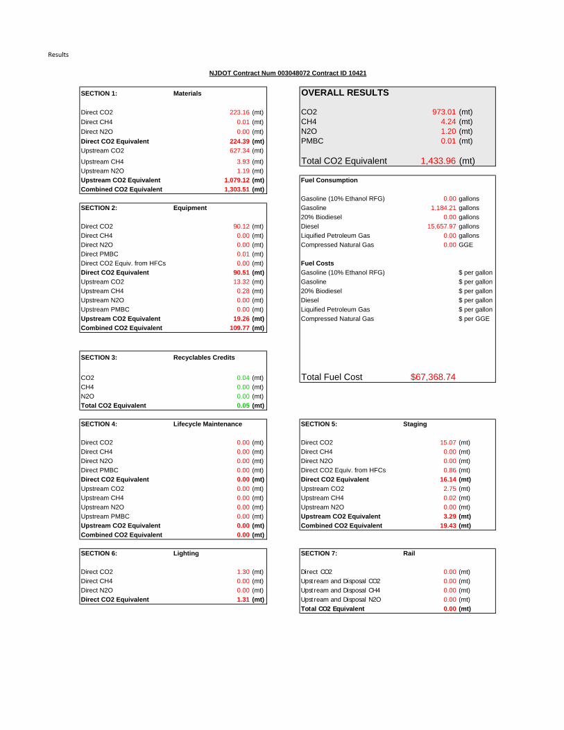
Results
SECTION 1: Materials OVERALL RESULTS
Direct CO2 223.16 (mt) CO2 973.01 (mt)Direct CH4 0.01 (mt) CH4 4.24 (mt)Direct N2O 0.00 (mt) N2O 1.20 (mt)Direct CO2 Equivalent 224.39 (mt) PMBC 0.01 (mt)Upstream CO2 627.34 (mt)
Upstream CH4 3.93 (mt) Total CO2 Equivalent 1,433.96 (mt)Upstream N2O 1.19 (mt)Upstream CO2 Equivalent 1,079.12 (mt) Fuel ConsumptionCombined CO2 Equivalent 1,303.51 (mt)
Gasoline (10% Ethanol RFG) 0.00 gallonsSECTION 2: Equipment Gasoline 1,184.21 gallons
20% Biodiesel 0.00 gallonsDirect CO2 90.12 (mt) Diesel 15,657.97 gallonsDirect CH4 0.00 (mt) Liquified Petroleum Gas 0.00 gallonsDirect N2O 0.00 (mt) Compressed Natural Gas 0.00 GGEDirect PMBC 0.01 (mt)Direct CO2 Equiv. from HFCs 0.00 (mt) Fuel CostsDirect CO2 Equivalent 90.51 (mt) Gasoline (10% Ethanol RFG) $ per gallonUpstream CO2 13.32 (mt) Gasoline $ per gallonUpstream CH4 0.28 (mt) 20% Biodiesel $ per gallonUpstream N2O 0.00 (mt) Diesel $ per gallonUpstream PMBC 0.00 (mt) Liquified Petroleum Gas $ per gallonUpstream CO2 Equivalent 19.26 (mt) Compressed Natural Gas $ per GGECombined CO2 Equivalent 109.77 (mt)
SECTION 3: Recyclables Credits
CO2 0.04 (mt) Total Fuel Cost $67,368.74CH4 0.00 (mt)N2O 0.00 (mt)Total CO2 Equivalent 0.05 (mt)
SECTION 4: Lifecycle Maintenance SECTION 5: Staging
Direct CO2 0.00 (mt) Direct CO2 15.07 (mt)Direct CH4 0.00 (mt) Direct CH4 0.00 (mt)Direct N2O 0.00 (mt) Direct N2O 0.00 (mt)Direct PMBC 0.00 (mt) Direct CO2 Equiv. from HFCs 0.86 (mt)Direct CO2 Equivalent 0.00 (mt) Direct CO2 Equivalent 16.14 (mt)Upstream CO2 0.00 (mt) Upstream CO2 2.75 (mt)Upstream CH4 0.00 (mt) Upstream CH4 0.02 (mt)Upstream N2O 0.00 (mt) Upstream N2O 0.00 (mt)Upstream PMBC 0.00 (mt) Upstream CO2 Equivalent 3.29 (mt)Upstream CO2 Equivalent 0.00 (mt) Combined CO2 Equivalent 19.43 (mt)Combined CO2 Equivalent 0.00 (mt)
SECTION 6: Lighting SECTION 7: Rail
Direct CO2 1.30 (mt) Direct CO2 0.00 (mt)Direct CH4 0.00 (mt) Upstream and Disposal CO2 0.00 (mt)Direct N2O 0.00 (mt) Upstream and Disposal CH4 0.00 (mt)Direct CO2 Equivalent 1.31 (mt) Upstream and Disposal N2O 0.00 (mt)
Total CO2 Equivalent 0.00 (mt)
NJDOT Contract Num 003048072 Contract ID 10421

Materials
Item Code Description Value Unit Cement Ratio Aggregate Ratio Heating Temp. % Binder % Moisture Cutback Depth (feet)
612006P Guide Sign, Type Ga, Steel "U" Post Supports 23.00 Sq. Feet N/A N/A N/A N/A N/A Non-Solvent-N/A N/A
612003P Regulatory And Warning Sign 406.00 Sq. Feet N/A N/A N/A N/A N/A Non-Solvent-N/A N/A
609039M Beam Guide Rail Anchorage 2.00 Units N/A N/A N/A N/A N/A Non-Solvent-N/A N/A
609027M Tangent Guide Rail Terminal 1.00 Units N/A N/A N/A N/A N/A Non-Solvent-N/A N/A
609024M Flared Guide Rail Terminal 1.00 Units N/A N/A N/A N/A N/A Non-Solvent-N/A N/A
609021M Rub Rail 650.00 Feet N/A N/A N/A N/A N/A Non-Solvent-N/A N/A
609003M Beam Guide Rail 825.00 Feet N/A N/A N/A N/A N/A Non-Solvent-N/A N/A
608004P Nonvegetative Surface, Porous Hot Mix Asphalt, 4" Thick 673.00 Sq. Yard N/A N/A N/A 0.04 0.04 Non-Solvent-N/A N/A
607069P 9" X Variable Height Concrete Vertical Curb 2,800.00 Feet 0.15 0.80 N/A N/A N/A Non-Solvent-N/A N/A
607018P 9" X 16" Concrete Vertical Curb 923.00 Feet 0.15 0.80 N/A N/A N/A Non-Solvent-N/A N/A
606075P Concrete Island, 4" Thick 93.00 Sq. Yard 0.15 0.80 N/A N/A N/A Non-Solvent-N/A N/A
606039P Hot Mix Asphalt Driveway, 6" Thick 475.00 Sq. Yard N/A N/A N/A 0.04 0.04 Non-Solvent-N/A N/A
602213M Curb Piece 24.00 Units N/A N/A N/A N/A N/A Non-Solvent-N/A 15.00
602054M Manhole, 4' Diameter 1.00 Units 0.15 0.80 N/A N/A N/A Non-Solvent-N/A 15.00
602013M Inlet, Type Double B 1.00 Units 0.15 0.80 N/A N/A N/A Non-Solvent-N/A 15.00
602012M Inlet, Type B 9.00 Units 0.15 0.80 N/A N/A N/A Non-Solvent-N/A 15.00
601122P 15" Reinforced Concrete Pipe 213.00 Feet N/A N/A N/A N/A N/A Non-Solvent-N/A N/A
401099M HMA - Base Course 385.00 Tons N/A N/A 325.00 0.04 0.04 Non-Solvent-N/A N/A
401078M HMA - Intermediate Course 6,660.00 Tons N/A N/A 325.00 0.04 0.04 Non-Solvent-N/A N/A
401072M HMA - Intermediate Course 220.00 Tons N/A N/A 325.00 0.04 0.04 Non-Solvent-N/A N/A
401048M HMA - Surface Course 4,000.00 Tons N/A N/A 325.00 0.05 0.04 Non-Solvent-N/A N/A
401036M Prime Coat, Cut-Back Asphalt 220.00 Gallons N/A N/A 120.00 N/A N/A MC-0.3 N/A
401030M Tack Coat 12,700.00 Gallons N/A N/A 145.00 N/A N/A Non-Solvent-0 N/A
304012P Concrete Base Course, 12" Thick 17.00 Sq. Yards 0.15 0.80 N/A N/A N/A Non-Solvent-N/A N/A
304009P Concrete Base Course, 10" Thick 284.00 Sq. Yards 0.15 0.80 N/A N/A N/A Non-Solvent-N/A N/A
302042P Dense-Graded Aggregate Base Course, 8" Thick 670.00 Sq. Yards N/A N/A N/A N/A N/A Non-Solvent-N/A N/A
302036P Dense-Graded Aggregate Base Course, 6" Thick 187.00 Sq. Yards N/A N/A N/A N/A N/A Non-Solvent-N/A N/A
Item Code Description Direct CO2 (g) Direct CH4 (g) Direct N2O (g) Direct CO2 Equiv. (g) Upstream CO2 (g) Upstream CH4 (g) Upstream N2O (g) Upstream CO2 Equiv. (g)
612006P Guide Sign, Type Ga, Steel "U" Post Supports 0.00 0.00 0.00 0.00 276,487.19 409.01 2.49 285,846.79
612003P Regulatory And Warning Sign 0.00 0.00 0.00 0.00 4,880,599.98 7,219.89 43.87 5,045,817.25
609039M Beam Guide Rail Anchorage 0.00 0.00 0.00 0.00 51,883.18 69.49 0.38 53,459.14
609027M Tangent Guide Rail Terminal 0.00 0.00 0.00 0.00 338,343.69 453.16 2.45 348,620.62
609024M Flared Guide Rail Terminal 0.00 0.00 0.00 0.00 338,343.69 453.16 2.45 348,620.62
609021M Rub Rail 0.00 0.00 0.00 0.00 36,268,727.87 46,630.45 247.52 37,324,699.68
609003M Beam Guide Rail 0.00 0.00 0.00 0.00 20,364,212.96 27,083.35 144.25 20,977,681.50
608004P Nonvegetative Surface, Porous Hot Mix Asphalt, 4" Thick 1,823,719.50 71.77 27.64 1,833,794.32 2,901,423.85 17,448.90 47.37 3,282,535.50
607069P 9" X Variable Height Concrete Vertical Curb 0.00 0.00 0.00 0.00 1,835,151.18 6,711.57 4,746.19 3,447,411.69
607018P 9" X 16" Concrete Vertical Curb 0.00 0.00 0.00 0.00 16,329,229.81 989,147.16 976,475.52 339,808,732.79
606075P Concrete Island, 4" Thick 0.00 0.00 0.00 0.00 3,515,663.48 2,313.35 359.13 3,675,575.06
606039P Hot Mix Asphalt Driveway, 6" Thick 1,930,758.02 75.98 29.26 1,941,424.15 3,071,715.44 18,473.01 50.15 3,475,195.46
602213M Curb Piece 0.00 0.00 0.00 0.00 4,483,756.38 3,306.34 15.14 4,557,881.40
602054M Manhole, 4' Diameter 0.00 0.00 0.00 0.00 5,952,168.34 5,559.15 149.76 6,115,337.68
602013M Inlet, Type Double B 0.00 0.00 0.00 0.00 6,161,911.92 5,480.79 228.87 6,347,956.60
602012M Inlet, Type B 0.00 0.00 0.00 0.00 55,457,207.29 49,327.07 2,059.79 57,131,609.41
601122P 15" Reinforced Concrete Pipe 0.00 0.00 0.00 0.00 9,529,387.98 202,093.10 192,754.12 73,527,121.46
401099M HMA - Base Course 7,462,709.49 293.68 113.09 7,503,935.91 11,872,704.81 71,401.35 193.84 13,432,223.99
401078M HMA - Intermediate Course 129,095,182.40 5,080.24 1,956.38 129,808,345.89 205,382,374.04 1,235,150.66 3,353.20 232,360,030.59
401072M HMA - Intermediate Course 4,264,405.42 167.82 64.63 4,287,963.38 6,784,402.75 40,800.77 110.77 7,675,556.57
401048M HMA - Surface Course 77,763,300.43 3,054.51 1,178.47 78,192,772.06 162,259,595.05 960,476.36 2,642.70 183,248,834.28
401036M Prime Coat, Cut-Back Asphalt 440,277.73 0.06 0.06 440,298.91 605,177.96 3,383.50 9.77 679,261.01
401030M Tack Coat 376,629.62 5.46 5.71 378,515.93 38,071,566.89 213,041.08 614.88 42,736,043.16
304012P Concrete Base Course, 12" Thick 0.00 0.00 0.00 0.00 1,927,944.49 1,268.61 196.94 2,015,637.94
304009P Concrete Base Course, 10" Thick 0.00 0.00 0.00 0.00 26,840,011.49 17,661.06 2,741.77 28,060,841.85
302042P Dense-Graded Aggregate Base Course, 8" Thick 0.00 0.00 0.00 0.00 1,524,168.29 1,141.78 3,433.42 2,612,506.81
302036P Dense-Graded Aggregate Base Course, 6" Thick 0.00 0.00 0.00 0.00 319,051.65 239.01 718.71 546,871.76

Equipment
Year Description Fuel Type Power Rating Hours Air Conditioning Direct CO2 (g) Direct CH4 (g) Direct N2O (g) Direct PMBC (g) Direct CO2 Equiv. from HFCs(g) Direct CO2 Equiv. (g)
2009 Cement & Mortar Mixers Diesel 75 60 No 907,215.26 5.29 11.37 138.94 0.00 910,851.52
2007 Cranes Diesel 750 35 No 5,346,971.98 27.79 74.51 519.20 0.00 5,370,652.64
2004 Pavers Diesel 600 300 No 36,764,258.82 197.67 506.76 4,448.14 0.00 36,925,505.92
2005 Paving Equipment Diesel 100 500 No 14,639,239.83 167.78 181.69 3,728.67 0.00 14,699,087.53
2008 Excavators Diesel 100 100 No 3,224,500.08 20.09 40.02 1,188.66 0.00 3,237,329.22
2007 Crawler Tractors Diesel 1000 100 No 29,235,726.42 187.70 402.98 3,465.92 0.00 29,364,592.40
Year Description Fuel Type Power Rating Hours Upstream CO2 (g)
Upstream CH4 (g)
Upstream N2O (g)
Upstream PMBC (g)
Upstream CO2 Equiv. (g) Fuel Use Fuel Unit
2009 Cement & Mortar Mixers Diesel 75 60 306,336.22 6,587.37 4.37 10.21 446,027.05 206.29 gallons
2007 Cranes Diesel 750 35 776,356.04 16,694.56 11.09 25.87 1,130,378.21 1,215.80 gallons
2004 Pavers Diesel 600 300 5,333,246.88 114,684.75 76.15 177.69 7,765,233.65 6,087.08 gallons
2005 Paving Equipment Diesel 100 500 2,125,767.20 45,711.94 30.35 70.82 3,095,127.48 2,426.24 gallons
2008 Excavators Diesel 100 100 537,129.15 5,097.67 12.78 25.57 648,142.78 534.45 gallons
2007 Crawler Tractors Diesel 1000 100 4,241,050.11 91,198.43 60.56 141.30 6,174,989.80 4,840.51 gallons
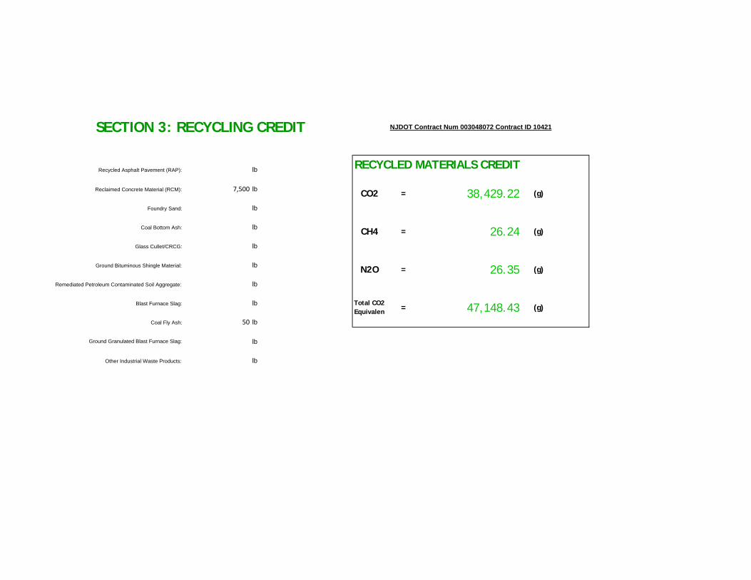
lb
7,500 lb
lb
lb
lb
lb
lb
lb
50 lb
lb
lb
Reclaimed Concrete Material (RCM): CO2 = 38,429.22 (g)
SECTION 3: RECYCLING CREDIT NJDOT Contract Num 003048072 Contract ID 10421
RECYCLED MATERIALS CREDITRecycled Asphalt Pavement (RAP):
(g)
Foundry Sand:
Coal Bottom Ash: CH4 = 26.24 (g)
Glass Cullet/CRCG:
Ground Bituminous Shingle Material: N2O = 26.35
Ground Granulated Blast Furnace Slag:
Remediated Petroleum Contaminated Soil Aggregate:
Blast Furnace Slag: Total CO2 Equivalen = 47,148.43 (g)
Other Industrial Waste Products:
Coal Fly Ash:
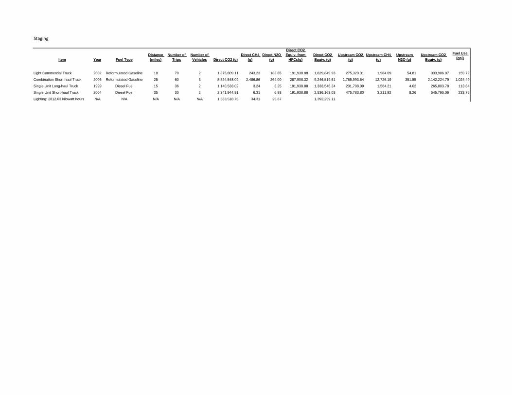
Staging
Item Year Fuel TypeDistance (miles)
Number of Trips
Number of Vehicles Direct CO2 (g)
Direct CH4 (g)
Direct N2O (g)
Direct CO2 Equiv. from
HFCs(g)Direct CO2 Equiv. (g)
Upstream CO2 (g)
Upstream CH4 (g)
Upstream N2O (g)
Upstream CO2 Equiv. (g)
Fuel Use (gal)
Light Commercial Truck 2002 Reformulated Gasoline 18 70 2 1,375,809.11 243.23 183.85 191,938.88 1,629,849.93 275,329.31 1,984.09 54.81 333,986.07 159.72
Combination Short-haul Truck 2006 Reformulated Gasoline 25 60 3 8,824,548.09 2,486.86 264.00 287,908.32 9,246,519.61 1,765,993.64 12,726.19 351.55 2,142,224.79 1,024.49
Single Unit Long-haul Truck 1999 Diesel Fuel 15 36 2 1,140,533.02 3.24 3.25 191,938.88 1,333,546.24 231,708.09 1,564.21 4.02 265,803.78 113.84
Single Unit Short-haul Truck 2004 Diesel Fuel 35 30 2 2,341,944.91 6.31 6.93 191,938.88 2,536,163.03 475,783.80 3,211.92 8.26 545,795.06 233.76
Lighting: 2812.03 kilowatt hours N/A N/A N/A N/A N/A 1,383,518.76 34.31 25.87 1,392,259.11
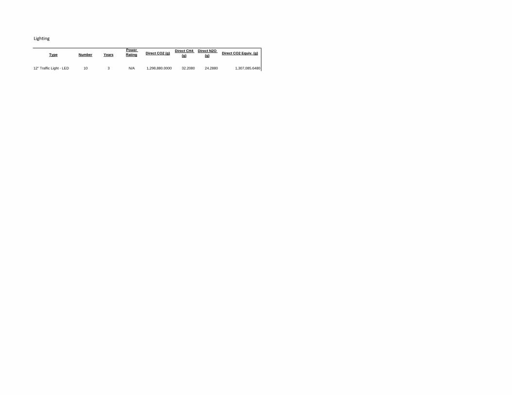
Lighting
Type Number YearsPower Rating Direct CO2 (g) Direct CH4
(g)Direct N2O
(g) Direct CO2 Equiv. (g)
12" Traffic Light - LED 10 3 N/A 1,298,880.0000 32.2080 24.2880 1,307,085.6480
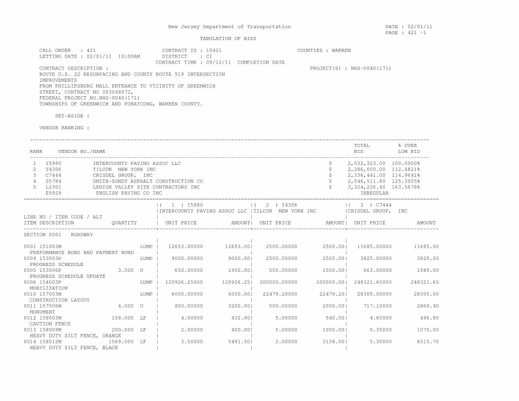
New Jersey Department of Transportation DATE : 02/01/11 PAGE : 421 -1 TABULATION OF BIDS CALL ORDER : 421 CONTRACT ID : 10421 COUNTIES : WARREN LETTING DATE : 02/01/11 10:00AM DISTRICT : C1 CONTRACT TIME : 09/12/11 COMPLETION DATE CONTRACT DESCRIPTION : PROJECT(S) : NHS-0040(171) ROUTE U.S. 22 RESURFACING AND COUNTY ROUTE 519 INTERSECTION IMPROVEMENTS FROM PHILLIPSBURG MALL ENTRANCE TO VICINITY OF GREENWICH STREET, CONTRACT NO 003048072, FEDERAL PROJECT NO.NHS-0040(171) TOWNSHIPS OF GREENWICH AND POHATCONG, WARREN COUNTY. SET-ASIDE : VENDOR RANKING : ------------------------------------------------------------------------------------------------------------------------------- TOTAL % OVER RANK VENDOR NO./NAME BID LOW BID ------------------------------------------------------------------------------------------------------------------------------- 1 I5980 INTERCOUNTY PAVING ASSOC LLC $ 2,032,323.00 100.0000% 2 T4306 TILCON NEW YORK INC $ 2,286,000.00 112.4821% 3 C7444 CRISDEL GROUP, INC $ 2,336,441.00 114.9641% 4 S5784 SMITH-SONDY ASPHALT CONSTRUCTION CO $ 2,546,511.80 125.3005% 5 L2301 LEHIGH VALLEY SITE CONTRACTORS INC $ 3,324,226.40 163.5678% E5929 ENGLISH PAVING CO INC IRREGULAR ==================================================================================================================================== |( 1 ) I5980 |( 2 ) T4306 |( 3 ) C7444 |INTERCOUNTY PAVING ASSOC LLC |TILCON NEW YORK INC |CRISDEL GROUP, INC LINE NO / ITEM CODE / ALT | | | ITEM DESCRIPTION QUANTITY | UNIT PRICE AMOUNT| UNIT PRICE AMOUNT| UNIT PRICE AMOUNT ------------------------------------------+-----------------------------+-----------------------------+----------------------------- SECTION 0001 ROADWAY | | | 0001 151003M LUMP | 12653.00000 12653.00| 2500.00000 2500.00| 11685.00000 11685.00 PERFORMANCE BOND AND PAYMENT BOND | | | 0004 153003P LUMP | 9000.00000 9000.00| 2500.00000 2500.00| 3825.00000 3825.00 PROGRESS SCHEDULE | | | 0005 153006P 3.000 U | 650.00000 1950.00| 500.00000 1500.00| 663.00000 1989.00 PROGRESS SCHEDULE UPDATE | | | 0006 154003P LUMP | 120926.25000 120926.25| 200000.00000 200000.00| 248321.65000 248321.65 MOBILIZATION | | | 0010 157003M LUMP | 6000.00000 6000.00| 22479.20000 22479.20| 28305.00000 28305.00 CONSTRUCTION LAYOUT | | | 0011 157006M 4.000 U | 800.00000 3200.00| 500.00000 2000.00| 717.10000 2868.40 MONUMENT | | | 0012 158003M 108.000 LF | 4.00000 432.00| 5.00000 540.00| 4.60000 496.80 CAUTION FENCE | | | 0013 158009M 200.000 LF | 2.00000 400.00| 5.00000 1000.00| 5.35000 1070.00 HEAVY DUTY SILT FENCE, ORANGE | | | 0014 158012M 1569.000 LF | 3.50000 5491.50| 2.00000 3138.00| 5.30000 8315.70 HEAVY DUTY SILT FENCE, BLACK | | |

New Jersey Department of Transportation DATE : 02/01/11 PAGE : 421 -2 TABULATION OF BIDS CALL ORDER : 421 CONTRACT ID : 10421 COUNTIES : WARREN LETTING DATE : 02/01/11 10:00AM DISTRICT : C1 SET-ASIDE : ==================================================================================================================================== |( 1 ) I5980 |( 2 ) T4306 |( 3 ) C7444 |INTERCOUNTY PAVING ASSOC LLC |TILCON NEW YORK INC |CRISDEL GROUP, INC LINE NO / ITEM CODE / ALT | | | ITEM DESCRIPTION QUANTITY | UNIT PRICE AMOUNT| UNIT PRICE AMOUNT| UNIT PRICE AMOUNT ------------------------------------------+-----------------------------+-----------------------------+----------------------------- 0015 158015M 25.000 U | 5.00000 125.00| 5.00000 125.00| 20.00000 500.00 HAYBALE | | | 0016 158030M 62.000 U | 95.00000 5890.00| 25.00000 1550.00| 120.80000 7489.60 INLET FILTER TYPE 2, 2' X 4' | | | 0017 158033M 11.000 U | 105.00000 1155.00| 25.00000 275.00| 198.55000 2184.05 INLET FILTER TYPE 2, 4' X 4' | | | 0018 158063P LUMP | 1500.00000 1500.00| 1000.00000 1000.00| 1836.00000 1836.00 CONCRETE WASHOUT SYSTEM | | | 0019 158072M 2.000 U | 1.00000 2.00| 450.00000 900.00| 816.00000 1632.00 OIL ONLY EMERGENCY SPILL KIT, TYPE 1 | | | 0020 158084M 70.000 CY | 1.00000 70.00| 5.00000 350.00| 58.30000 4081.00 EROSION CONTROL SEDIMENT REMOVAL | | | 0021 159003M 100.000 U | 1.00000 100.00| 1.00000 100.00| 0.01000 1.00 BREAKAWAY BARRICADE | | | 0022 159006M 300.000 U | 0.01000 3.00| 1.00000 300.00| 0.01000 3.00 DRUM | | | 0023 159009M 150.000 U | 15.00000 2250.00| 20.00000 3000.00| 0.01000 1.50 TRAFFIC CONE | | | 0024 159012M 1380.000 SF | 1.00000 1380.00| 5.00000 6900.00| 16.40000 22632.00 CONSTRUCTION SIGNS | | | 0025 159018M 2.000 U | 1000.00000 2000.00| 900.00000 1800.00| 2020.70000 4041.40 CONSTRUCTION IDENTIFICATION SIGN, 6' X | | | 12' | | | 0026 159027M 4.000 U | 250.00000 1000.00| 500.00000 2000.00| 1.05000 4.20 FLASHING ARROW BOARD, 4' X 8' | | | 0027 159030M 5.000 U | 2000.00000 10000.00| 1000.00000 5000.00| 3671.90000 18359.50 PORTABLE VARIABLE MESSAGE SIGN | | | 0028 159108M 2.000 U | 50000.00000 100000.00| 6000.00000 12000.00| 13709.05000 27418.10 TRAFFIC CONTROL TRUCK WITH MOUNTED | | | CRASH CUSHION | | | 0029 159126M 16870.000 LF | 0.25000 4217.50| 0.36000 6073.20| 0.25000 4217.50 TEMPORARY TRAFFIC STRIPES, 4" | | | 0030 159132M 1000.000 SF | 1.05000 1050.00| 1.00000 1000.00| 1.00000 1000.00 TEMPORARY PAVEMENT MARKINGS | | | 0031 159135M 350.000 U | 1.55000 542.50| 1.50000 525.00| 2.05000 717.50 TEMPORARY PAVEMENT MARKERS | | | 0032 159138M 40.000 T | 1.00000 40.00| 150.00000 6000.00| 85.20000 3408.00 HMA PATCH | | | 0033 159141M 500.000 HOUR | 75.00000 37500.00| 65.00000 32500.00| 1.00000 500.00 TRAFFIC DIRECTOR, FLAGGER | | |

New Jersey Department of Transportation DATE : 02/01/11 PAGE : 421 -3 TABULATION OF BIDS CALL ORDER : 421 CONTRACT ID : 10421 COUNTIES : WARREN LETTING DATE : 02/01/11 10:00AM DISTRICT : C1 SET-ASIDE : ==================================================================================================================================== |( 1 ) I5980 |( 2 ) T4306 |( 3 ) C7444 |INTERCOUNTY PAVING ASSOC LLC |TILCON NEW YORK INC |CRISDEL GROUP, INC LINE NO / ITEM CODE / ALT | | | ITEM DESCRIPTION QUANTITY | UNIT PRICE AMOUNT| UNIT PRICE AMOUNT| UNIT PRICE AMOUNT ------------------------------------------+-----------------------------+-----------------------------+----------------------------- 0034 159144M 5.000 U | 1.00000 5.00| 75.00000 375.00| 255.00000 1275.00 EMERGENCY TOWING SERVICE | | | 0035 160003M LUMP | 2300.00000 2300.00| 2300.00000 2300.00| 2300.00000 2300.00 FUEL PRICE ADJUSTMENT | | | 0036 160006M LUMP | 11700.00000 11700.00| 11700.00000 11700.00| 11700.00000 11700.00 ASPHALT PRICE ADJUSTMENT | | | 0037 161003P LUMP | 5500.00000 5500.00| 5000.00000 5000.00| 4859.65000 4859.65 FINAL CLEANUP | | | 0038 162003M 1.000 U | 1300.00000 1300.00| 2000.00000 2000.00| 2364.10000 2364.10 CONDITION SURVEY | | | 0039 201003P LUMP | 5250.00000 5250.00| 5000.00000 5000.00| 18582.80000 18582.80 CLEARING SITE | | | 0040 202006M 10.000 CY | 1.00000 10.00| 100.00000 1000.00| 581.85000 5818.50 EXCAVATION, TEST PIT | | | 0041 202009P 234.000 CY | 22.00000 5148.00| 100.00000 23400.00| 49.60000 11606.40 EXCAVATION, UNCLASSIFIED | | | 0042 202021P 1328.000 SY | 4.00000 5312.00| 50.00000 66400.00| 39.15000 51991.20 REMOVAL OF PAVEMENT | | | 0043 203041P 670.000 SY | 1.50000 1005.00| 4.00000 2680.00| 1.90000 1273.00 GEOTEXTILE, ROADWAY STABILIZATION | | | 0044 302036P 187.000 SY | 7.50000 1402.50| 25.00000 4675.00| 9.70000 1813.90 DENSE-GRADED AGGREGATE BASE COURSE, 6" | | | THICK | | | 0045 302042P 670.000 SY | 15.00000 10050.00| 15.00000 10050.00| 19.85000 13299.50 DENSE-GRADED AGGREGATE BASE COURSE, 8" | | | THICK | | | 0046 304009P 284.000 SY | 1.00000 284.00| 100.00000 28400.00| 71.40000 20277.60 CONCRETE BASE COURSE, 10" THICK | | | 0047 304012P 17.000 SY | 1.00000 17.00| 115.00000 1955.00| 81.60000 1387.20 CONCRETE BASE COURSE, 12" THICK | | | 0048 401009P 37726.000 SY | 1.50000 56589.00| 3.00000 113178.00| 2.95000 111291.70 HMA MILLING, 3" OR LESS GRADE CONTROLLE | | | 0049 401012P 3018.000 SY | 2.00000 6036.00| 3.00000 9054.00| 4.65000 14033.70 HMA MILLING, MORE THAN 3" TO 6" GRADE | | | CONTROLLED | | | 0050 401021M 50.000 SY | 1.00000 50.00| 110.00000 5500.00| 74.35000 3717.50 HOT MIX ASPHALT PAVEMENT REPAIR | | | 0051 401027M 26500.000 LF | 0.35000 9275.00| 0.01000 265.00| 0.35000 9275.00 POLYMERIZED JOINT ADHESIVE | | |

New Jersey Department of Transportation DATE : 02/01/11 PAGE : 421 -4 TABULATION OF BIDS CALL ORDER : 421 CONTRACT ID : 10421 COUNTIES : WARREN LETTING DATE : 02/01/11 10:00AM DISTRICT : C1 SET-ASIDE : ==================================================================================================================================== |( 1 ) I5980 |( 2 ) T4306 |( 3 ) C7444 |INTERCOUNTY PAVING ASSOC LLC |TILCON NEW YORK INC |CRISDEL GROUP, INC LINE NO / ITEM CODE / ALT | | | ITEM DESCRIPTION QUANTITY | UNIT PRICE AMOUNT| UNIT PRICE AMOUNT| UNIT PRICE AMOUNT ------------------------------------------+-----------------------------+-----------------------------+----------------------------- 0052 401030M 12700.000 GAL | 0.01000 127.00| 1.00000 12700.00| 0.01000 127.00 TACK COAT | | | 0053 401036M 220.000 GAL | 0.01000 2.20| 1.00000 220.00| 0.01000 2.20 PRIME COAT | | | 0054 401042M 110.000 T | 51.50000 5665.00| 100.00000 11000.00| 94.60000 10406.00 HOT MIX ASPHALT 9.5 M 64 SURFACE COURSE | | | 0055 401048M 4000.000 T | 70.75000 283000.00| 80.00000 320000.00| 75.55000 302200.00 HOT MIX ASPHALT 9.5 M 76 SURFACE COURSE | | | 0056 401072M 220.000 T | 52.75000 11605.00| 100.00000 22000.00| 94.60000 20812.00 HOT MIX ASPHALT 12.5 M 64 INTERMEDIATE | | | COURSE | | | 0057 401078M 6660.000 T | 70.00000 466200.00| 80.00000 532800.00| 73.50000 489510.00 HOT MIX ASPHALT 12.5 M 76 INTERMEDIATE | | | COURSE | | | 0058 401099M 385.000 T | 64.59000 24867.15| 100.00000 38500.00| 96.35000 37094.75 HOT MIX ASPHALT 25 M 64 BASE COURSE | | | 0059 401108M 50.000 U | 50.00000 2500.00| 50.00000 2500.00| 86.65000 4332.50 CORE SAMPLES, HOT MIX ASPHALT | | | 0060 453006M 100.000 SY | 1.00000 100.00| 175.00000 17500.00| 311.00000 31100.00 FULL DEPTH CONCRETE PAVEMENT REPAIR, HM | | | 0061 456003M 8100.000 LF | 0.01000 81.00| 1.50000 12150.00| 1.55000 12555.00 SEALING EXISTING JOINTS IN CONCRETE | | | PAVEMENT | | | 0062 601122P 213.000 LF | 260.00000 55380.00| 150.00000 31950.00| 176.60000 37615.80 15" REINFORCED CONCRETE PIPE | | | 0064 602012M 9.000 U | 2500.00000 22500.00| 2900.00000 26100.00| 4426.40000 39837.60 INLET, TYPE B | | | 0065 602013M 1.000 U | 6800.00000 6800.00| 4100.00000 4100.00| 6947.95000 6947.95 INLET, TYPE DOUBLE B | | | 0066 602054M 1.000 U | 2400.00000 2400.00| 2500.00000 2500.00| 4353.60000 4353.60 MANHOLE, 4' DIAMETER | | | 0067 602099M 43.000 U | 900.00000 38700.00| 250.00000 10750.00| 751.60000 32318.80 RESET EXISTING CASTING | | | 0068 602108M 2.000 U | 1550.00000 3100.00| 1400.00000 2800.00| 1260.95000 2521.90 SET INLET TYPE E, CASTING | | | 0069 602213M 24.000 U | 250.00000 6000.00| 450.00000 10800.00| 333.30000 7999.20 CURB PIECE | | | 0070 606039P 475.000 SY | 58.00000 27550.00| 50.00000 23750.00| 62.15000 29521.25 HOT MIX ASPHALT DRIVEWAY, 6" THICK | | |

New Jersey Department of Transportation DATE : 02/01/11 PAGE : 421 -5 TABULATION OF BIDS CALL ORDER : 421 CONTRACT ID : 10421 COUNTIES : WARREN LETTING DATE : 02/01/11 10:00AM DISTRICT : C1 SET-ASIDE : ==================================================================================================================================== |( 1 ) I5980 |( 2 ) T4306 |( 3 ) C7444 |INTERCOUNTY PAVING ASSOC LLC |TILCON NEW YORK INC |CRISDEL GROUP, INC LINE NO / ITEM CODE / ALT | | | ITEM DESCRIPTION QUANTITY | UNIT PRICE AMOUNT| UNIT PRICE AMOUNT| UNIT PRICE AMOUNT ------------------------------------------+-----------------------------+-----------------------------+----------------------------- 0071 606075P 93.000 SY | 74.00000 6882.00| 87.00000 8091.00| 88.75000 8253.75 CONCRETE ISLAND, 4" THICK | | | 0072 607018P 923.000 LF | 29.15000 26905.45| 34.50000 31843.50| 16.30000 15044.90 9" X 16" CONCRETE VERTICAL CURB | | | 0073 607069P 2800.000 LF | 30.25000 84700.00| 36.00000 100800.00| 18.35000 51380.00 9" X VARIABLE HEIGHT CONCRETE VERTICAL | | | CURB | | | 0074 608004P 673.000 SY | 26.25000 17666.25| 26.00000 17498.00| 25.50000 17161.50 NONVEGETATIVE SURFACE, POROUS HOT MIX | | | ASPHALT, 4" THICK | | | 0075 609003M 825.000 LF | 18.91000 15600.75| 19.45000 16046.25| 18.35000 15138.75 BEAM GUIDE RAIL | | | 0076 609021M 650.000 LF | 6.80000 4420.00| 6.50000 4225.00| 6.65000 4322.50 RUB RAIL | | | 0077 609024M 1.000 U | 2300.00000 2300.00| 2325.00000 2325.00| 2295.00000 2295.00 FLARED GUIDE RAIL TERMINAL | | | 0078 609027M 1.000 U | 2300.00000 2300.00| 2400.00000 2400.00| 2295.00000 2295.00 TANGENT GUIDE RAIL TERMINAL | | | 0079 609039M 2.000 U | 630.00000 1260.00| 454.00000 908.00| 612.00000 1224.00 BEAM GUIDE RAIL ANCHORAGE | | | 0080 609075M 896.000 LF | 1.00000 896.00| 2.60000 2329.60| 1.00000 896.00 REMOVAL OF BEAM GUIDE RAIL | | | 0081 610003M 13300.000 LF | 0.32000 4256.00| 0.30000 3990.00| 0.30000 3990.00 TRAFFIC STRIPES, LONG LIFE, EPOXY RESIN | | | 4" | | | 0082 610007M 3800.000 LF | 0.58000 2204.00| 0.55000 2090.00| 0.55000 2090.00 TRAFFIC STRIPES, LONG LIFE, EPOXY RESIN | | | 8" | | | 0083 610009M 3600.000 SF | 2.60000 9360.00| 2.50000 9000.00| 2.55000 9180.00 TRAFFIC MARKINGS, THERMOPLASTIC | | | 0084 610012M 315.000 U | 25.20000 7938.00| 24.00000 7560.00| 24.50000 7717.50 RPM, MONO-DIRECTIONAL, WHITE LENS | | | 0085 610018M 95.000 U | 25.20000 2394.00| 24.00000 2280.00| 24.50000 2327.50 RPM, MONO-DIRECTIONAL, AMBER LENS | | | 0086 610021M 10.000 U | 25.20000 252.00| 24.00000 240.00| 24.50000 245.00 RPM, BI-DIRECTIONAL, AMBER LENS | | | 0087 612003P 406.000 SF | 56.25000 22837.50| 27.00000 10962.00| 30.60000 12423.60 REGULATORY AND WARNING SIGN | | | 0088 612006P 23.000 SF | 42.00000 966.00| 52.50000 1207.50| 40.80000 938.40 GUIDE SIGN, TYPE GA, STEEL "U" POST | | | SUPPORTS | | |
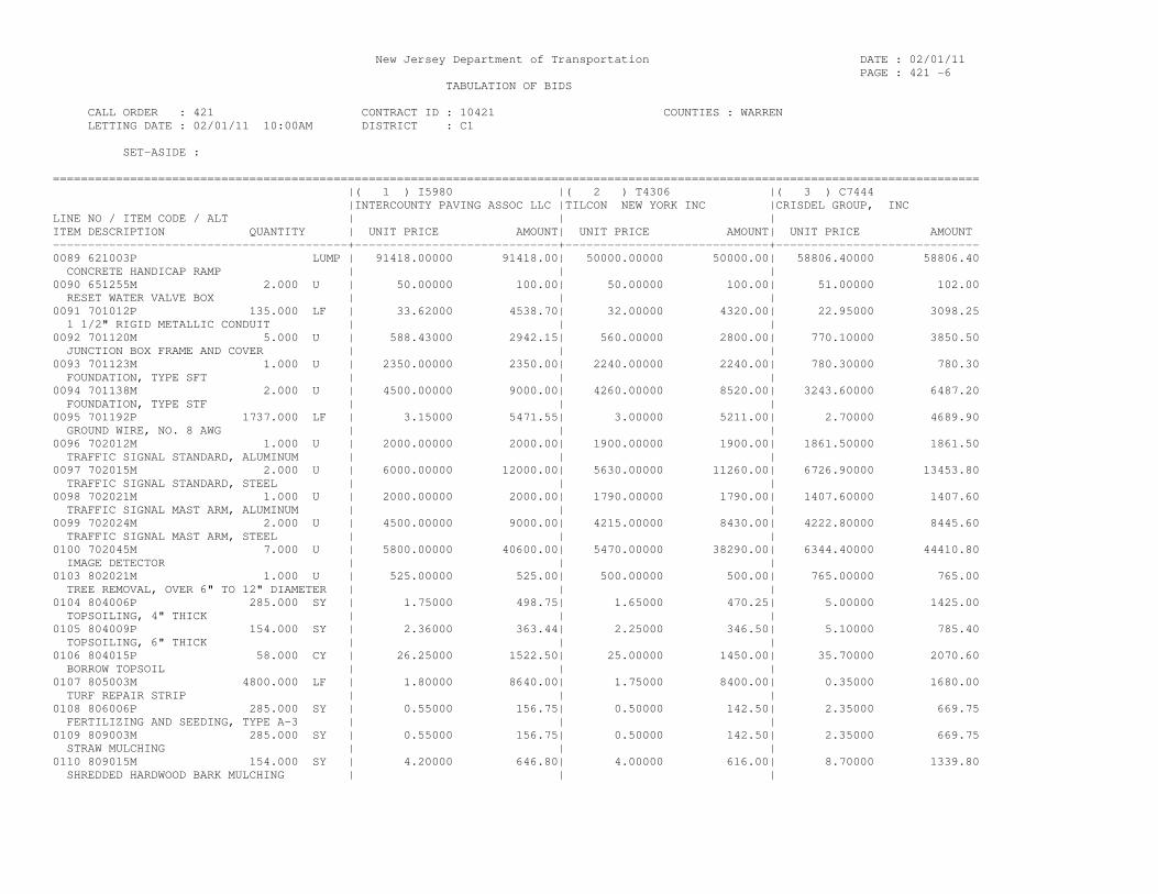
New Jersey Department of Transportation DATE : 02/01/11 PAGE : 421 -6 TABULATION OF BIDS CALL ORDER : 421 CONTRACT ID : 10421 COUNTIES : WARREN LETTING DATE : 02/01/11 10:00AM DISTRICT : C1 SET-ASIDE : ==================================================================================================================================== |( 1 ) I5980 |( 2 ) T4306 |( 3 ) C7444 |INTERCOUNTY PAVING ASSOC LLC |TILCON NEW YORK INC |CRISDEL GROUP, INC LINE NO / ITEM CODE / ALT | | | ITEM DESCRIPTION QUANTITY | UNIT PRICE AMOUNT| UNIT PRICE AMOUNT| UNIT PRICE AMOUNT ------------------------------------------+-----------------------------+-----------------------------+----------------------------- 0089 621003P LUMP | 91418.00000 91418.00| 50000.00000 50000.00| 58806.40000 58806.40 CONCRETE HANDICAP RAMP | | | 0090 651255M 2.000 U | 50.00000 100.00| 50.00000 100.00| 51.00000 102.00 RESET WATER VALVE BOX | | | 0091 701012P 135.000 LF | 33.62000 4538.70| 32.00000 4320.00| 22.95000 3098.25 1 1/2" RIGID METALLIC CONDUIT | | | 0092 701120M 5.000 U | 588.43000 2942.15| 560.00000 2800.00| 770.10000 3850.50 JUNCTION BOX FRAME AND COVER | | | 0093 701123M 1.000 U | 2350.00000 2350.00| 2240.00000 2240.00| 780.30000 780.30 FOUNDATION, TYPE SFT | | | 0094 701138M 2.000 U | 4500.00000 9000.00| 4260.00000 8520.00| 3243.60000 6487.20 FOUNDATION, TYPE STF | | | 0095 701192P 1737.000 LF | 3.15000 5471.55| 3.00000 5211.00| 2.70000 4689.90 GROUND WIRE, NO. 8 AWG | | | 0096 702012M 1.000 U | 2000.00000 2000.00| 1900.00000 1900.00| 1861.50000 1861.50 TRAFFIC SIGNAL STANDARD, ALUMINUM | | | 0097 702015M 2.000 U | 6000.00000 12000.00| 5630.00000 11260.00| 6726.90000 13453.80 TRAFFIC SIGNAL STANDARD, STEEL | | | 0098 702021M 1.000 U | 2000.00000 2000.00| 1790.00000 1790.00| 1407.60000 1407.60 TRAFFIC SIGNAL MAST ARM, ALUMINUM | | | 0099 702024M 2.000 U | 4500.00000 9000.00| 4215.00000 8430.00| 4222.80000 8445.60 TRAFFIC SIGNAL MAST ARM, STEEL | | | 0100 702045M 7.000 U | 5800.00000 40600.00| 5470.00000 38290.00| 6344.40000 44410.80 IMAGE DETECTOR | | | 0103 802021M 1.000 U | 525.00000 525.00| 500.00000 500.00| 765.00000 765.00 TREE REMOVAL, OVER 6" TO 12" DIAMETER | | | 0104 804006P 285.000 SY | 1.75000 498.75| 1.65000 470.25| 5.00000 1425.00 TOPSOILING, 4" THICK | | | 0105 804009P 154.000 SY | 2.36000 363.44| 2.25000 346.50| 5.10000 785.40 TOPSOILING, 6" THICK | | | 0106 804015P 58.000 CY | 26.25000 1522.50| 25.00000 1450.00| 35.70000 2070.60 BORROW TOPSOIL | | | 0107 805003M 4800.000 LF | 1.80000 8640.00| 1.75000 8400.00| 0.35000 1680.00 TURF REPAIR STRIP | | | 0108 806006P 285.000 SY | 0.55000 156.75| 0.50000 142.50| 2.35000 669.75 FERTILIZING AND SEEDING, TYPE A-3 | | | 0109 809003M 285.000 SY | 0.55000 156.75| 0.50000 142.50| 2.35000 669.75 STRAW MULCHING | | | 0110 809015M 154.000 SY | 4.20000 646.80| 4.00000 616.00| 8.70000 1339.80 SHREDDED HARDWOOD BARK MULCHING | | |
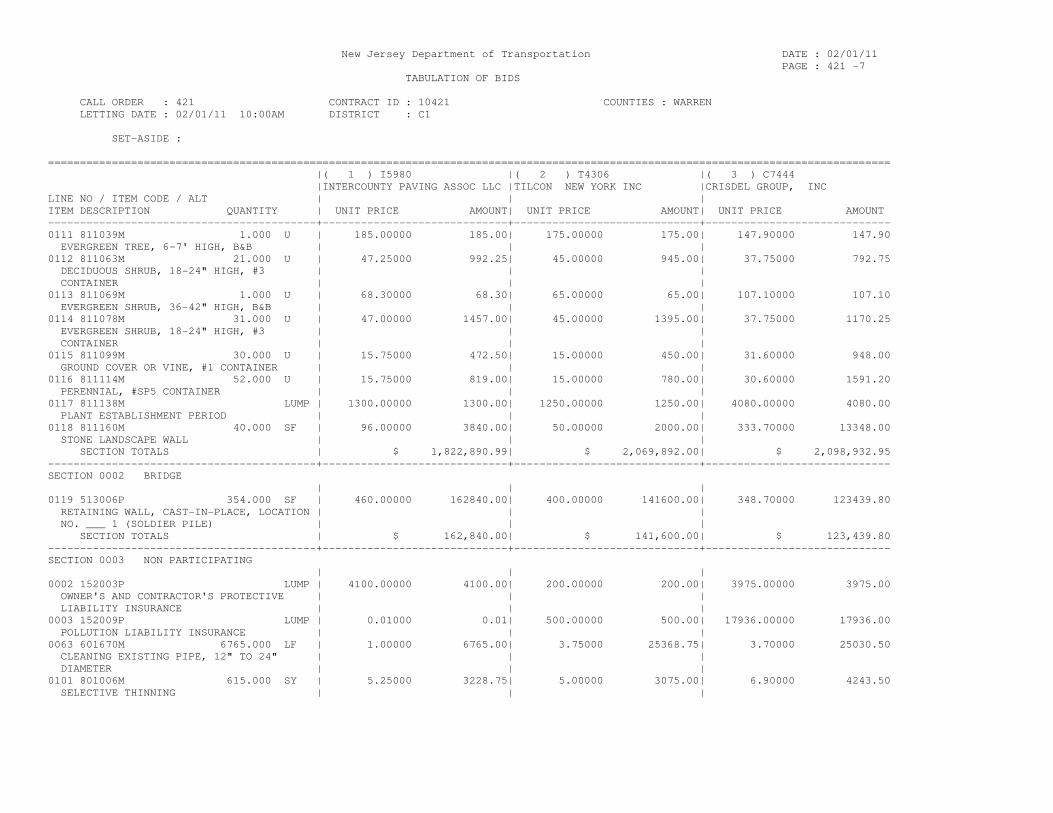
New Jersey Department of Transportation DATE : 02/01/11 PAGE : 421 -7 TABULATION OF BIDS CALL ORDER : 421 CONTRACT ID : 10421 COUNTIES : WARREN LETTING DATE : 02/01/11 10:00AM DISTRICT : C1 SET-ASIDE : ==================================================================================================================================== |( 1 ) I5980 |( 2 ) T4306 |( 3 ) C7444 |INTERCOUNTY PAVING ASSOC LLC |TILCON NEW YORK INC |CRISDEL GROUP, INC LINE NO / ITEM CODE / ALT | | | ITEM DESCRIPTION QUANTITY | UNIT PRICE AMOUNT| UNIT PRICE AMOUNT| UNIT PRICE AMOUNT ------------------------------------------+-----------------------------+-----------------------------+----------------------------- 0111 811039M 1.000 U | 185.00000 185.00| 175.00000 175.00| 147.90000 147.90 EVERGREEN TREE, 6-7' HIGH, B&B | | | 0112 811063M 21.000 U | 47.25000 992.25| 45.00000 945.00| 37.75000 792.75 DECIDUOUS SHRUB, 18-24" HIGH, #3 | | | CONTAINER | | | 0113 811069M 1.000 U | 68.30000 68.30| 65.00000 65.00| 107.10000 107.10 EVERGREEN SHRUB, 36-42" HIGH, B&B | | | 0114 811078M 31.000 U | 47.00000 1457.00| 45.00000 1395.00| 37.75000 1170.25 EVERGREEN SHRUB, 18-24" HIGH, #3 | | | CONTAINER | | | 0115 811099M 30.000 U | 15.75000 472.50| 15.00000 450.00| 31.60000 948.00 GROUND COVER OR VINE, #1 CONTAINER | | | 0116 811114M 52.000 U | 15.75000 819.00| 15.00000 780.00| 30.60000 1591.20 PERENNIAL, #SP5 CONTAINER | | | 0117 811138M LUMP | 1300.00000 1300.00| 1250.00000 1250.00| 4080.00000 4080.00 PLANT ESTABLISHMENT PERIOD | | | 0118 811160M 40.000 SF | 96.00000 3840.00| 50.00000 2000.00| 333.70000 13348.00 STONE LANDSCAPE WALL | | | SECTION TOTALS | $ 1,822,890.99| $ 2,069,892.00| $ 2,098,932.95 ------------------------------------------+-----------------------------+-----------------------------+----------------------------- SECTION 0002 BRIDGE | | | 0119 513006P 354.000 SF | 460.00000 162840.00| 400.00000 141600.00| 348.70000 123439.80 RETAINING WALL, CAST-IN-PLACE, LOCATION | | | NO. ___ 1 (SOLDIER PILE) | | | SECTION TOTALS | $ 162,840.00| $ 141,600.00| $ 123,439.80 ------------------------------------------+-----------------------------+-----------------------------+----------------------------- SECTION 0003 NON PARTICIPATING | | | 0002 152003P LUMP | 4100.00000 4100.00| 200.00000 200.00| 3975.00000 3975.00 OWNER'S AND CONTRACTOR'S PROTECTIVE | | | LIABILITY INSURANCE | | | 0003 152009P LUMP | 0.01000 0.01| 500.00000 500.00| 17936.00000 17936.00 POLLUTION LIABILITY INSURANCE | | | 0063 601670M 6765.000 LF | 1.00000 6765.00| 3.75000 25368.75| 3.70000 25030.50 CLEANING EXISTING PIPE, 12" TO 24" | | | DIAMETER | | | 0101 801006M 615.000 SY | 5.25000 3228.75| 5.00000 3075.00| 6.90000 4243.50 SELECTIVE THINNING | | |

New Jersey Department of Transportation DATE : 02/01/11 PAGE : 421 -8 TABULATION OF BIDS CALL ORDER : 421 CONTRACT ID : 10421 COUNTIES : WARREN LETTING DATE : 02/01/11 10:00AM DISTRICT : C1 SET-ASIDE : ==================================================================================================================================== |( 1 ) I5980 |( 2 ) T4306 |( 3 ) C7444 |INTERCOUNTY PAVING ASSOC LLC |TILCON NEW YORK INC |CRISDEL GROUP, INC LINE NO / ITEM CODE / ALT | | | ITEM DESCRIPTION QUANTITY | UNIT PRICE AMOUNT| UNIT PRICE AMOUNT| UNIT PRICE AMOUNT ------------------------------------------+-----------------------------+-----------------------------+----------------------------- 0102 801012M 333.000 SY | 5.25000 1748.25| 7.25000 2414.25| 10.20000 3396.60 SELECTIVE CLEARING | | | SECTION TOTALS | $ 15,842.01| $ 31,558.00| $ 54,581.60 ------------------------------------------+-----------------------------+-----------------------------+----------------------------- SECTION 0004 CONSTRUCTION ENGINEERING | | | 0007 155006M 1.000 U | 15000.00000 15000.00| 20000.00000 20000.00| 28549.15000 28549.15 FIELD OFFICE TYPE B SET UP | | | 0008 155024M 9.000 MO | 1500.00000 13500.00| 2300.00000 20700.00| 3187.50000 28687.50 FIELD OFFICE TYPE B MAINTENANCE | | | 0009 155039M LUMP | 2250.00000 2250.00| 2250.00000 2250.00| 2250.00000 2250.00 TELEPHONE SERVICE | | | SECTION TOTALS | $ 30,750.00| $ 42,950.00| $ 59,486.65 ------------------------------------------+-----------------------------+-----------------------------+----------------------------- CONTRACT TOTALS | $ 2,032,323.00| $ 2,286,000.00| $ 2,336,441.00 ==================================================================================================================================== I CERTIFY THAT THE ABOVE IS AN EXACT TRANSCRIPT OF THE ORIGINAL BID PROPOSAL, EXCEPT THAT ERRORS, IF ANY, IN EXTENSION AND ADDITIONS HAVE BEEN CORRECTED. SIGNED,

269
APPENDIX I: RAIL CASE STUDIES
Case study data were obtained from New Jersey Transit (NJT).95 An older atlas of NJT commuter rail lines (New Jersey Transit 1993) was obtained and provides the basis of our analysis of the Morristown line, the Montclair line, the Princeton line, the Bergen County line, and the Pascack Valley line. In addition bid-sheets were obtained from New Jersey Transit for three rail stations including Lindenwold station, the Pennsauken Transit Center, and Ridgewood station. The modeling assumptions are fully presented in the section of the report entitled Data and Assumptions for a Life-Cycle Greenhouse Gas Analysis of Rail Transit Capital Projects. These case studies are aimed at demonstrating the applicability of using readily available transit data to evaluate the life-cycle greenhouse gas (GHG) emissions from construction projects. We document the information that is available for various commuter rail lines in New Jersey and evaluate its usefulness. GHG emissions from the construction of track, overhead catenary structures, tunnels, bridges, passenger stations, parking facilities, and rolling stock are included in our analysis. New Jersey Transit Commuter Lines
At the suggestion of a contact at New Jersey Transit, data for NJT commuter lines were taken from (New Jersey Transit 1993) that presents commuter lines as schematic diagrams called map pages. The diagrams show single, double, triple, and quadruple track, electrified and non-electrified portions, tunnels, bridges, and passenger stations. They are drawn to scale. Pedestrian tunnels and overpasses are shown, as are cross streets, overpasses, and water features. Mile markers and distance from the origin are shown for most features. Crossovers are shown but not included because they are clearly not to scale and are not quantifiable. Power supply substations are shown but not included because they are accounted for as part of the catenary systems. Table 42 shows the quantified components for these five NJT commuter rail lines, while the figures that follow show the relative contribution of each major component. Because this is commuter rail we assume that rail size is 115 lbs/yd and that concrete ties are used. As with DRTD light rail we assume that the material inputs from catenary systems are multiplied by the number of tracks for the portions of track that are doubled, tripled, or quadrupled, as are tunnel miles and bridge miles. We assume that whenever rail crosses over a street, undivided highway, small water feature, or a pedestrian tunnel that a bridge of 0.01 miles (52.8 feet) is constructed. The length of bridges over divided highways is doubled. Larger water features are assessed by an approximation of their apparent size on the map provided by NJT. We make a large assumption by assuming that bridges are drawn to scale, however distances measured by mile marker positions and feature locations suggest that the diagrams are drawn to scale. Consistent with our methodology, all stations are assumed to be of the platform type. We recognize that 95 This component of the work was also a contribution to TCRP H41.

270
many stations have structures, but information on these was unavailable. Parking facility capacity is estimated from the NJT 2010 Parking Guide (New Jersey Transit 2010). This document establishes the number of parking spaces at each station but does not apportion them between surface parking lots and structured parking garages. We established garage and surface lot parking from various sources. No information about rolling stock was available from our sources. Track spurs and private facilities are not included in our analysis.
Table 42. GHG Emissions from Five New Jersey Transit Commuter Rail Lines.
Morristown Line - Commuter Rail CO2 CH4 N2O GWP Tonnes Tonnes Tonnes Tonnes Type of Rail Commuter Track miles 121.8 146,929.0 137.484 21.774 156,566.2 Electrified track miles 94.92 589,311.0 744.961 4.806 606,445.0 Tunnel miles 7 336,097.1 225.723 11.330 344,349.6 Bridge miles 1.2 86,132.4 80.058 3.508 88,901.2 Platforms 25 10,539.0 9.655 0.789 10,986.2 Parking lot spaces 6,055 1,134.5 2.709 0.018 1,197.0 Parking garage spaces 906 9,791.7 8.837 0.756 10,211.7 Total 1,179,934.6 1,209.427 42.982 1,218,657.0 Princeton Line - Commuter Rail CO2 CH4 N2O GWP Tonnes Tonnes Tonnes Tonnes Type of Rail Commuter Track miles 3.75 4,523.7 4.233 0.670 4,820.4 Electrified track miles 3.75 23,281.9 29.431 0.190 23,958.8 Tunnel miles 0 0.0 0.000 0.000 0.0 Bridge miles 0.01 717.8 0.667 0.029 740.8 Platforms 2 843.1 0.772 0.063 878.9 Parking lot spaces 285 53.4 0.128 0.001 56.3 Parking garage spaces 0 0.0 0.000 0.000 0.0 Total 29,419.8 35.231 0.953 30,455.3 Pascack Valley Line CO2 CH4 N2O GWP Tonnes Tonnes Tonnes Tonnes Type of Rail Commuter Track miles 24.15 29,132.5 27.260 4.317 31,043.3 Electrified track miles 0 0.0 0.000 0.000 0.0 Tunnel miles 0 0.0 0.000 0.000 0.0 Bridge miles 0.06 4,306.6 4.003 0.175 4,445.1 Platforms 16 6,744.9 6.179 0.505 7,031.2 Parking lot spaces 2,042 382.6 0.914 0.006 403.7 Parking garage spaces 0 0.0 0.000 0.000 0.0 Total 40,566.6 38.355 5.004 42,923.2 Montclair Line - Commuter Rail CO2 CH4 N2O GWP Tonnes Tonnes Tonnes Tonnes Type of Rail Commuter Track miles 7.81 9,421.3 8.816 1.396 10,039.3 Electrified track miles 7.81 48,488.4 61.295 0.395 49,898.2 Tunnel miles 0 0.0 0.000 0.000 0.0 Bridge miles 0.20 14,355.4 13.343 0.585 14,816.9 Platforms 4 1,686.2 1.545 0.126 1,757.8
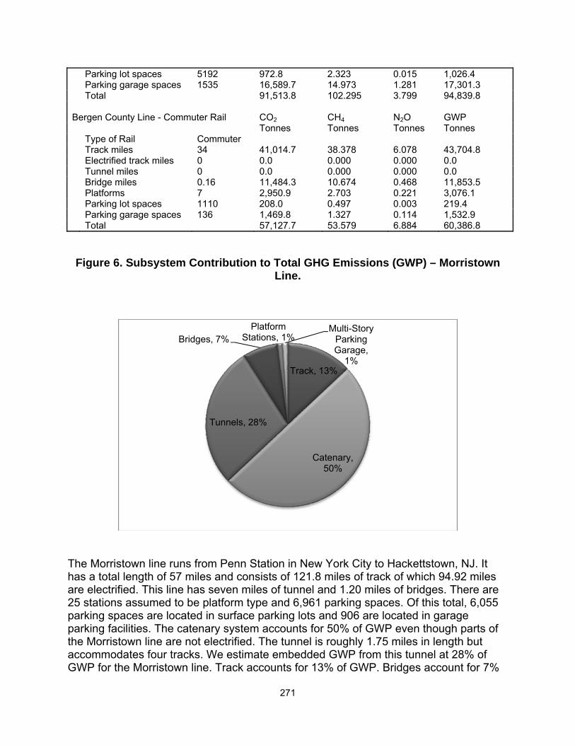
271
Parking lot spaces 5192 972.8 2.323 0.015 1,026.4 Parking garage spaces 1535 16,589.7 14.973 1.281 17,301.3 Total 91,513.8 102.295 3.799 94,839.8 Bergen County Line - Commuter Rail CO2 CH4 N2O GWP Tonnes Tonnes Tonnes Tonnes Type of Rail Commuter Track miles 34 41,014.7 38.378 6.078 43,704.8 Electrified track miles 0 0.0 0.000 0.000 0.0 Tunnel miles 0 0.0 0.000 0.000 0.0 Bridge miles 0.16 11,484.3 10.674 0.468 11,853.5 Platforms 7 2,950.9 2.703 0.221 3,076.1 Parking lot spaces 1110 208.0 0.497 0.003 219.4 Parking garage spaces 136 1,469.8 1.327 0.114 1,532.9 Total 57,127.7 53.579 6.884 60,386.8
Figure 6. Subsystem Contribution to Total GHG Emissions (GWP) – Morristown Line.
The Morristown line runs from Penn Station in New York City to Hackettstown, NJ. It has a total length of 57 miles and consists of 121.8 miles of track of which 94.92 miles are electrified. This line has seven miles of tunnel and 1.20 miles of bridges. There are 25 stations assumed to be platform type and 6,961 parking spaces. Of this total, 6,055 parking spaces are located in surface parking lots and 906 are located in garage parking facilities. The catenary system accounts for 50% of GWP even though parts of the Morristown line are not electrified. The tunnel is roughly 1.75 miles in length but accommodates four tracks. We estimate embedded GWP from this tunnel at 28% of GWP for the Morristown line. Track accounts for 13% of GWP. Bridges account for 7%
Track, 13%
Catenary, 50%
Tunnels, 28%
Bridges, 7%Platform
Stations, 1%Multi-Story
Parking Garage,
1%
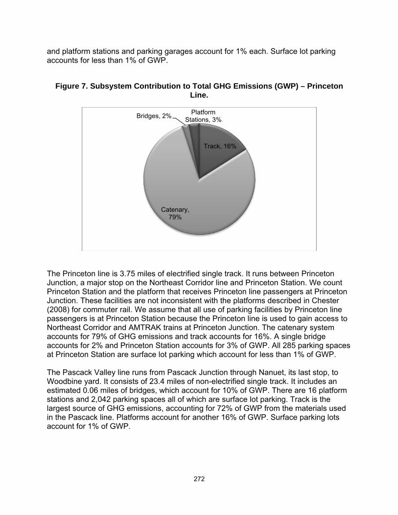
272
and platform stations and parking garages account for 1% each. Surface lot parking accounts for less than 1% of GWP.
Figure 7. Subsystem Contribution to Total GHG Emissions (GWP) – Princeton Line.
The Princeton line is 3.75 miles of electrified single track. It runs between Princeton Junction, a major stop on the Northeast Corridor line and Princeton Station. We count Princeton Station and the platform that receives Princeton line passengers at Princeton Junction. These facilities are not inconsistent with the platforms described in Chester (2008) for commuter rail. We assume that all use of parking facilities by Princeton line passengers is at Princeton Station because the Princeton line is used to gain access to Northeast Corridor and AMTRAK trains at Princeton Junction. The catenary system accounts for 79% of GHG emissions and track accounts for 16%. A single bridge accounts for 2% and Princeton Station accounts for 3% of GWP. All 285 parking spaces at Princeton Station are surface lot parking which account for less than 1% of GWP. The Pascack Valley line runs from Pascack Junction through Nanuet, its last stop, to Woodbine yard. It consists of 23.4 miles of non-electrified single track. It includes an estimated 0.06 miles of bridges, which account for 10% of GWP. There are 16 platform stations and 2,042 parking spaces all of which are surface lot parking. Track is the largest source of GHG emissions, accounting for 72% of GWP from the materials used in the Pascack line. Platforms account for another 16% of GWP. Surface parking lots account for 1% of GWP.
Track, 16%
Catenary, 79%
Bridges, 2% Platform Stations, 3%

273
Figure 8. Subsystem Contribution to Total GHG Emissions (GWP) – Pascack Valley Line.
Figure 9. Subsystem Contribution to Total GHG Emissions (GWP) – Montclair Line.
The Montclair line connects with the Morristown line near the Roseville substation. It has a total length of 4.12 miles from the connection with the Morristown line to Montclair station and includes three intermediate station stops. The track is double for 3.69 miles and single for 0.43 miles on either end of the line. The track is electrified along its entire length. We assume 7.81 track miles. Ten small road and small water feature crossings account for 0.20 bridge miles. There are four commuter rail platforms and 6,727 parking
Track, 72%
Bridges, 10%
Platform Stations, 16%
Surface Parking Lot,
1%
Track, 11%
Catenary, 53%
Bridges, 16%
Platform Stations, 2%
Surface Parking Lot,
1% Multi-Story Parking
Garage, 18%

274
spaces. Of these, 5,192 parking spaces are located in surface parking lots and 1,535 are located in garage parking facilities. The catenary system accounts for 53% of GWP from materials. Garage parking accounts for 18% of GWP, bridges account for 16% of GWP and track accounts for 11%. Platform stations account for 2% and surface parking lots account for 1% of GWP.
Figure 10. Subsystem Contribution to Total GHG Emissions (GWP) – Bergen County Line.
The Bergen County line leaves the Main Line at Bergen Junction and rejoins it at Ridgewood Junction. The track is doubled along its entire 17 mile length. The track is not electrified and there are no tunnels. We estimate 0.16 bridge miles, including a drawbridge over the Hackensack River drawn with an apparent length of 0.03 miles (158.6 feet) on the diagram. There are seven stations assumed to be platforms and 1,246 parking spaces. Surface parking lots account for 1,110 parking spaces and the remaining 136 parking spaces are located in garage parking facilities. Track accounts for 72% of GWP from material inputs and bridges account for 20%. Passenger stations account for 5% of GWP and garage parking accounts for 3%. Surface parking lots account for less than 1% of GWP. Table 43 shows our estimates for the ranges of total GHG emissions per mile for four NJT commuter rail systems. Two of the lines, Princeton and Montclair, are fully electrified. Two others, Pascack Valley and Bergen County are not electrified. The Morristown line, which is partially electrified is not shown. The range of the non-electrified lines is quite small. The range of the electrified lines is larger due to the relative abundance of garage parking on the Montclair line. Our analysis shows that catenary systems account for most GHG emissions on a material basis where they are present. On non-electrified track the track itself is generally the largest source of GHG
Track, 72%
Bridges, 20%
Platform Stations, 5%
Garage Parking, 3%

275
emissions. Tunnels and bridges, although they do not generally account for large portions of track represent relatively massive material inputs over short distances. Percent emissions from passenger stations are minor when track is electrified. All commuter rail stations are assumed to be of the platform type. These account for between one and two percent of GWP of electrified rail systems. On non-electrified track commuter rail station embedded GHG emissions are overshadowed to the extent that there are bridges and tunnels on the system. Parking spaces did not account for more than one percent of GHG emissions where garage parking was not present. This is largely due to the larger GHG emissions from garage parking per parking space in comparison with surface parking lots. The GWP of GHG increases 57 fold when a parking garage space is substituted for a surface lot parking space.
Table 43. Ranges of Estimated GWP for Electrified and Non-Electrified NJT Commuter Rail Systems.
GWP (tonnes per mile) Electrified Rail Princeton Line 8,121.40 Montclair Line 12,143.39 Non-electrified Rail Bergen County Line 1,776.08 Pascack Valley Line 1,777.36
New Jersey Transit Bid-sheets
We evaluated whether it was feasible to estimate emissions using a bottom-up approach, based on the components specified in contract bid-sheets. We received three contract bid-sheets for station construction/renovation that were provided by NJT. Detailed data on the material inputs would allow us to estimate the life-cycle emissions associated with each. These need to be provided based on material weight or volume with known densities. Measures used in construction contracts commonly awarded by the New Jersey Department of Transportation are generally quantifiable. They may be stated as volumes, such as cubic feet of concrete, reinforced concrete, aggregate or asphalt. They may also be stated as weight, such as pounds of steel, or aluminum. Areas may be used to a known depth, such as square yards of pavement, or metal plating. Linear distance may be used for which the material for which weight or volume has been worked out for a known distance, as we have done with ballast. Pipe, guard rails, and fencing are examples of the latter. After reviewing the three contract bid-sheets it was clear that a bottom-up approach would not work for any of them. Two of the contracts (Pennsauken Transit Center and Lindenwold Station) do not present any quantifiable material inputs. The third contract (Ridgewood Station) specifies most material inputs as lump sums. This is problematic because the material inputs are not quantified.

276
The contract bid-sheet items that are unquantifiable include items that are exclusively equipment activity inputs. These include such things as site clearing, disposal, drainage, saw-cutting, drilling, grading, excavation, embankment building, and landscaping. To quantify these inputs we could use EPA’s NONROAD application with an inventory of the equipment used including fuel type, power rating for each equipment piece, and ideally vintage year. In addition we would need to know either fuel consumption or duration of operation, or as an alternative, a quantified expression of the work performed with each piece of equipment, such as cubic yards of material excavated, linear feet of a hole drilled to a known diameter, or square yards of pavement broken up. This latter type of information can be theoretically interpreted in a rough sense based on production rates per hour, which are often found on equipment specifications. The Lindenwold contract specifies linear feet of drilled shafts of two and three-foot diameters. These could be interpreted if we knew the power rating, fuel type, and production rate of the drill or drills used. Many of the material inputs are not quantifiable. Lump sums are specified for sub-base courses, sidewalks, curbs, ballast, cast-in-place and precast concrete, concrete wearing surfaces, glass pavers, structural steel, handrails, timber, tiles, sheet metal, doors of a variety of materials, trims of various kinds, and so on. The Lindenwold contract specifies square yards of broken stone surface course, but not the depth. The specification of square feet of non-slip membrane coating is quantifiable but we have not identified the material. The under platform fence and chain link fencing, expressed as linear feet, could be easily quantified if we knew the height. Assuming a default mixture cast-in-place concrete expressed as cubic yards is easily quantifiable, as are brick masonry walls and concrete block expressed in square feet. Retractable platform edges and timber bumper strips expressed in linear feet are not quantifiable. Our conclusion is that that most of the material inputs in these station contracts are not fully quantifiable. To successfully accomplish the type of inventory we attempted with data readily available from New Jersey Transit it would be necessary to work from the engineering plans and schematic diagrams. Conclusions
We have examined data obtained from two sources in an attempt to establish what sorts of information might be readily available conduct GHG inventories of rail construction projects. It is impossible to discuss what we have done as a full GHG inventory because we have not been able to present equipment activity data, except for averages for drilling in tunnel construction. An ideal approach is to first quantify the material inputs and then assess the embedded energy and process emissions for each material. These emissions are largely upstream in nature; the fugitive process emissions are the only direct emissions. These can be readily calculated for all major material components. One key input that is missing is that data is not available on construction equipment activity. Specifically, equipment use data would need to be collected either based on fuel consumption or on the total number of hours of equipment operation. Other necessary equipment parameters are fuel type, power rating, and

277
some approximation of average load. To accomplish such a study from the bottom up these data are indispensible. Equipment emissions factors are readily available from NONROAD if these data were available. Based on our experience with these data it is clear that most analyses of GHG emissions from rail system construction will be based on averages, similar to what we have done. The data from New Jersey Transit include, at best, totals of track miles that are either at grade, below grade, or above grade, as well as the proportion of track that is electrified and supported by bridges or tunnels. The material inputs of stations of a handful of types are assumed based on totals from other rail systems. We are able to estimate track based on a bottom up approach, but no other rail system component. Our attempt to estimate the material inputs of rail passenger stations was not successful. Significant changes will be necessary in the ways that transit agencies present data before valid construction-related greenhouse gas inventories are possible.

278
279
APPENDIX J: REFERENCES
AASHTO 2007, "Roadway Maintenance and Management" in AASHTO Maintenance Manual for Roadways and Bridges., 4th Edition edn, American Association of State Highway and Transportation Officials, Washington, DC.
Abraham, H. 1945, Asphalts and Allied Substances, Vol. 2, Fifth Edition edn, C. Van Nostrand Company, Inc., New York.
Agency for Toxic Substances and Disease Registry 2010, Toxological Substances – Creosote. Available April 15, 2011 at http://www.atsdr.cdc.gov/toxprofiles/tp.asp?id=66&tid=18.
AISI 2009, , How A Blast Furnace Works [Homepage of American Iron and Steel Institute], [Online]. Available: http://www.steel.org/AM/Template.cfm?Section=Articles3&CONTENTID=25317&TEMPLATE=/CM/ContentDisplay.cfm [2009, 11/12/2009].
AISI 2007, CO2 Breakthrough Projects. [AISI webpage]. Available April 30, 2010 at http://www.steel.org/AM/Template.cfm?Section=Fact_Sheets2&TEMPLATE=/CM/HTMLDisplay.cfm&CONTENTID=18071.
American Concrete Pipe Association 1970, Concrete Pipe Design Manual 3rd edn, .
Andersen, J.P. & Hyman, B. 2001, "Energy and Material Flow Models for the US Steel Industry", Energy, vol. 26, pp. 137-159.
Andreae, M.O. & Gelenscér, A. 2006, "Black Carbon or Brown Carbon? The Nature of Light-Absorbing Carbonaceous Aerosols.", Atmospheric Chemistry and Physics, vol. 6, pp. 3131-3148.
Andress, D. 2002, Soil Carbon Changes for Bioenergy Crops, David Andress & Associates, Inc., Kensington, MD.
AREMA 2000b, Manual for Railway Engineering, Chapter 4, American Railway Engineering and Maintenance-of-Way Association, Lanham, MD.
AREMA 2000a, Manual for Railway Engineering, Chapter 1 , American Railway Engineering and Maintenance-of-Way Association, Lanham, MD.
Argonne National Laboratory 2009, GREET 1.8c Fuel Cycle Model., Argonne National Laboratory.
Argonne National Laboratory 2007, GREET 2.7 Vehicle Cycle Model, Argonne National Laboratory.

280
Arnott, R. & Small, K. 1994, "The economics of traffic congestion", American Scientist, vol. 82, pp. 446-446.
Baker, J. 2003, "Greenhouse Gas Emissions from Vehicle Air Conditioning Systems", International Vehicle Technology Symposium, Sacramento, CA, March 11-13.
Baker, J. 1999, Mobile air conditioning: HFC-134a emissions and emissions reduction strategies, UNEP TEAP HFC/PFC Task Force, Delphi Automotive Systems, Inc.
Barr, L.C. 2000, "Testing for the significance of induced highway travel demand in metropolitan areas", Transportation Research Record: Journal of the Transportation Research Board, vol. 1706, no. -1, pp. 1-8.
Barrault, S., Benouali, J. & Clodic, D. 2003, Analysis of the economic and environmental consequences of a phase out or considerable reduction leakage of mobile air conditioners, European Commission.
Barth, M., An, F., Norbeck, J. & Ross, M. 1996, "Modal emissions modeling: a physical approach", Transportation Research Record: Journal of the Transportation Research Board, vol. 1520, no. -1, pp. 81-88.
Barth, M., An, F., Younglove, T., Levine, C., Scora, G., Ross, M. & Wenzel, T. 1999, The Development of Comprehensive Modal Emissions Model.
Battye, W., Boyer, K. & Pace, T.G. 2002, Methods for Improving Global Inventories of Black Carbon and Organic Carbon Particulates, Environmental Protection Agency, Washington, DC.
BCS, I. 2002a, Energy and Environmental Profile of the U.S. Mining Industry. Chapter 4. Available April 22, 2010 at http://www1.eere.energy.gov/industry/mining/pdfs/iron.pdf. US Department of Energy. Office of Energy Efficiency and Renewable Energy, Washington, DC.
BCS, I. 2002b, Energy and Environmental Profile of the U.S. Mining Industry, US Department of Energy, Office of Energy Efficiency and Renewable Energy.
Buckingham, D.A., Plunkert, P.A. & Bray, E.L. 2010, Aluminum Statistics, 1900-2009. Available April 13, 2011 at http://minerals.usgs.gov/ds/2005/140/aluminum.pdf. USGS. Mineral Resources Program.
Budikova, D. 2010, January 24-last update, Encyclopedia of the Earth - Albedo. Available: www.eoearth.org/article/albedo [2010, 5/5].

281
Burnette, A. & Baker, R. A Study of R134a Leaks in Heavy Duty Vehicles accessed at www.arb.ca.gov/research/seminars/baker3/baker3.pdf.
Burnham, A., Wang, M. & Wu, Y. 2006, Development and Applications of GREET 2.7 - The Transportation Vehicle-Cycle Model, Center for Transportation Research, Argonne National Laboratory.
Cervero, R. 1988, Land-Use Mixing and Suburban Mobility.
Cervero, R. & Hansen, M. 2002, "Induced travel demand and induced road investment: A simultaneous equation analysis", Journal of Transport Economics and Policy (JTEP), vol. 36, no. 3, pp. 469-490.
Cervero, R. 2003, "Road expansion, urban growth, and induced travel: a path analysis", Journal of the American Planning Association, vol. 69, no. 2, pp. 145-164.
Cervero, R. 2002, "Induced travel demand: research design, empirical evidence, and normative policies", Journal of Planning Literature, vol. 17, no. 1, pp. 3.
Cervero, R. 1990, "Transit pricing research", Transportation, vol. 17, no. 2, pp. 117-139.
Chang, J.S. 2006, "Models of the relationship between transport and land-use: A review", Transport Reviews, vol. 26, no. 3, pp. 325-350.
Chester, M.V. 2008, Life-cycle Environmental Inventory of Passenger Transportation in the United States. Available April 15, 2011 at http://escholarship.org/uc/item/7n29n303. , Institute of Transportation Studies, UC Berkeley.
Choate, W.T. 2003, Energy and Emission Reduction Opportunities for the Cement Industry, US Department of Energy, Office of Energy Efficiency and Renewable Energy.
City of Chicago 2010, , Chicago Green Alley Handbook. Available: http://egov.cityofchicago.org/webportal/COCWebPortal/COC_EDITORIAL/GreenAlleyHandbook_Jan.pdf [2010, 5/5].
Clemeña, G.G. 1972, Determination of the Cement Content of Hardened Concrete by Selective Solution., Virgina Highway Research Council, Charlottesville, VA.
Climate Registry 2008, General Reporting Protocol: Version 1.1, The Climate Registry.
D'Angelo, J., Harm, E., Bartoszek, J., Baumgardner, G.C., M., Cowsert, J. & et al. 2008, Warm-Mix Asphalt: European Practice., American Trade Initiatives, Alexandria, VA.

282
DeCorla-Souza, P. 2000, "Induced highway travel: Transportation policy implications for congested metropolitan areas", Transportation Quarterly, vol. 54, no. 2, pp. 13-30.
DeCorla-Souza, P. & Cohen, H. 2009, , Accounting for Induced Travel in Evaluation of Urban Highway Expansion [Homepage of Federal Highway Administration], [Online]. Available: http://www.fhwa.dot.gov/steam/doc.htm [2009, 7/24].
DeCorla-Souza, P. & Cohen, H. 1998, "Accounting for Induced Travel in Evaluation of Metropolitan Highway Expansion", Preprint for the 77 th Annual Meeting of the Transportation Research Board. National Research Council, Washington, DC.
DeCorla-Souza, P. & Hunt, J.D. 1999, , Use of STEAM in Evaluating Transportation Alternatives. Available: http://www.fhwa.dot.gov/steam/steam-it.pdf [2009, 8/3].
Delucchi, M.A. 2003, A Lifecycle Emissions Model (LEM): Lifecycle Emissions from Transportation Fuels, Motor Vehicles, Transportation Modes, Electricity Use, Heating and Cooking Fuels, and Materials., Institute of Transportation Studies, University of California at Davis, Davis, CA.
Dowling, R., Ireson, R., Skabardonis, A., Gillen, D. & Stopher, P. 2005, Predicting Air Quality Effects of Traffic Improvements: Final Report and User's Guide, NCHRP Report 535 edn, Transportation Research Board, Washington DC.
Downs, A. 1992, Stuck in traffic: Coping with peak-hour expressway congestion, Brookings Institution, Washington, DC.
Edelstein, D.L. 2011, Mineral Commodity Summaries. Copper. Available April 13, 2011 at http://minerals.usgs.gov/minerals/pubs/commodity/copper/mcs-2008-coppe.pdf. USGS.
Elcock, D. 2007, Life-Cycle Thinking for the Oil and Gas Exploration and Production Industry, Argonne National Laboratory, Argonne, IL.
EPA 2010a, , Emissions Factors & AP 42, Compilation of Air Pollutant Emission Factors [Homepage of US Environmental Protection Agency], [Online]. Available: http://www.epa.gov/ttnchie1/ap42/ [2010, July].
EPA 2010b, EPA Finalizes Regulations for the National Renewable Fuel Standard Program for 2010 and Beyond, Environmental Protection Agency, Washington DC.
EPA 2010c, 5/6-last update, Heat Island Demonstration Projects. Available: http://yosemite.epa.gov/gw/statepolicyactions.nsf/HIRIInitiative?OpenView&count=500&type=Demonstration%20Project. [2010, 5/6].
EPA 2010d, Motor Vehicle Emission Simulator (MOVES), Environmental Protection Agency, Washington, DC.

283
EPA 2009a, Frequently Asked Questions About NONROAD2008, Environmental Protection Agency, Office of Transportation Equality, Washington, DC.
EPA 2009b, Inventory of U.S. Greenhouse Gas Emissions and Sinks: 1990-2007., Environmental Protection Agency.
EPA 2008a, NONROAD, EPA, Office of Transportation and Air Quality, Washington, DC.
EPA 2008b, Reducing Urban Heat Islands: Compendium of Strategies.
EPA 2005a, Conversion Factors for Hydrocarbon Emission Components, EPA, Office of Transportation and Air Quality, Washington, DC.
EPA 2005b, Exhaust Emission Factors for Nonroad Engine Modeling: Spark-Ignition, EPA, Office of Transportation and Air Quality, Washington, DC.
EPA 2005c, Geographic Allocation of Nonroad Engine Population Data to the State and County Level, EPA, Office of Transportation and Air Quality, Washington, DC.
EPA 2005d, Nonroad Engine Population Estimates, EPA, Office of Transportation and Air Quality, Washington, DC.
EPA 2005e, Nonroad Evaporative Emission Rates, EPA, Office of Transportation and Air Quality, Washington, DC.
EPA 2005f, Nonroad Spark-Ignition Engine Emission Deterioration Factors, EPA, Office of Transportation and Air Quality, Washington, DC.
EPA 2005g, Streamlined Life-Cycle Greenhouse Gas Emission Factors for Copper Wire.
EPA 2004a, Exhaust and Crankcase Emission Factors for Nonroad Engine Modeling--Compression-Ignition, EPA, Office of Transportation and Air Quality, Washington, DC.
EPA 2004b, Median Life, Annual Activity, and Load Factor Values for Nonroad Engine Emissions Modeling, EPA, Office of Transportation and Air Quality, Washington, DC.
EPA 2004c, Refueling Emissions for Nonroad Engine Modeling, EPA, Office of Transportation and Air Quality, Washington, DC.
EPA 2003, Background Document for Life-Cycle Greenhouse Gas Emission Factors for Clay Brick Reuse and Concrete Recycling.
284
EPA 1979, "4.5 Asphalt Paving Operations." in AP42, Compilation of Air Pollutant Emission Factors, Volume 1, Fifth Edition edn, Environmental Protection Agency, Washington DC.
Ewing, R. & Cervero, R. 2010, "Travel and the built environment", Journal of the American Planning Association, vol. 76, no. 3.
FHWA 1999, 6/14/1999-last update, Portland Cement [Homepage of Federal Highway Administration], [Online]. Available: http://fhwa.dot.gov/infrastructure/materialsgrp/cement.html [2010, 4/28].
FHWA , Stormwater Best Management Practices in an Ultra-Urban Setting, Porous Pavement Fact Sheet. Available: http://environment.fhwa.dot.gov/ecosystems/ultraurb/index.asp [2010, 5/5].
Forsyth, A., Krizek, K.J. & Rodríguez, D.A. 2009, "Non-motorized travel research and contemporary planning initiatives", Progress in Planning, vol. 71, no. 4, pp. 170-183.
Frank, L.D., Kerr, J., Sallis, J.F., Miles, R. & Chapman, J. 2008, "A hierarchy of sociodemographic and environmental correlates of walking and obesity", Preventive medicine, vol. 47, no. 2, pp. 172-178.
Frank, L.D., Saelens, B.E., Powell, K.E. & Chapman, J.E. 2007, "Stepping towards causation: Do built environments or neighborhood and travel preferences explain physical activity, driving, and obesity?", Social science & medicine, vol. 65, no. 9, pp. 1898-1914.
Frank, L.D. & Stone, B. 2000, "Linking land use with household vehicle emissions in the central Puget Sound: methodological framework and findings", Transportation Research Part D: Transport and Environment, vol. 5, no. 3, pp. 173-196.
Fuller, F.M. 1983, Engineering of pile installations, McGraw-Hill.
Fulton, L.M., Noland, R.B., Meszler, D.J. & Thomas, J.V. 2000, "A statistical analysis of induced travel effects in the US mid-Atlantic region", Journal of Transportation and Statistics, vol. 3, no. 1, pp. 1-14.
Gallivan, F. 2010, Greenhouse Gas Mitigation Measures for Transportation Construction, Maintenance and Operation Activities , NCHRP Project 25-25, Task 58 edn, National Research Council, Washington, DC.
Gerdes, K. & Skone, T.J. 2008a, Development of Baseline Data and Analysis of Life Cycle Greenhouse Gas Emissions of Petroleum-Based Fuels., National Energy Technology Laboratory, Pittsburgh, PA.

285
Gerdes, K. & Skone, T.J. 2008b, Development of Baseline Data and Analysis of Life Cycle Greenhouse Gas Emissions of Petroleum-Based Fuels., National Energy Technology Laboratory, Pittsburgh, PA.
Goodwin, P., Dargay, J. & Hanly, M. 2004, "Elasticities of road traffic and fuel consumption with respect to price and income: a review", Transport Reviews, vol. 24, no. 3, pp. 275-292.
Goodwin, P.B. 1996, "Empirical evidence on induced traffic", Transportation, vol. 23, no. 1, pp. 35-54.
Goodwin, P. 1992, "A review of new demand elasticities with special reference to short and long run effects of price changes", Journal of Transport Economics and Policy, , pp. 155-169.
Gorham, R. 2009, Demystifying Induced Travel Demand, Sustainable Urban Transport Technical Document #1 edn, Deutche Gesellschaft, Eschborn, Germany.
Graham, D.J. 2007, "Variable returns to agglomeration and the effect of road traffic congestion", Journal of Urban Economics, vol. 62, no. 1, pp. 103-120.
Greenhalgh, S., Broekhoff, D., Daviet, F., Ranganathan, J., Acharya, M., Corbier, L., Oren, K. & Sundin, H. 2005, The Greenhouse Gas Protocol for Project Accounting, The World Resources Institute and World Business Council for Sustainable Development, Washington, DC.
Greer, W.L., Dougherty, A. & Sweeney, D.M. 2000, Air Pollution Engineering Manual. Second Edition edn, John Wiley and Sons, New York.
Guggemos, A.A. & Horvath, A. 2005, "Comparison of Environmental Effects of Steel- and Concrete-Framed Buildings", Journal of Infrastructure Systems, vol. 11, no. 2, pp. 93-101.
Guo, J., Bhat, C. & Copperman, R. 2007, "Effect of the Built Environment on Motorized and Nonmotorized Trip Making: Substitutive, Complementary, or Synergistic?", Transportation Research Record: Journal of the Transportation Research Board, vol. 2010, no. -1, pp. 1-11.
Handy, S., Cao, X. & Mokhtarian, P.L. 2006, "Self-selection in the relationship between the built environment and walking: Empirical evidence from Northern California", Journal of the American Planning Association, vol. 72, no. 1, pp. 55-74.
Hansen, M., Gillen, D., Dobbins, A., Huang, Y. & Puvathingal, M. 1993, "The air quality impacts of urban highway capacity expansion: Traffic generation and land use change", Institute of Transportation Studies, University of California, Berkeley, .

286
Hansen, M. & Huang, Y. 1997, "Road supply and traffic in California urban areas", Transportation Research Part A, vol. 31, no. 3, pp. 205-218.
Hawk, H. 2003, Bridge Life-Cycle Cost Analysis, Transportation Research Board, Washington, DC.
Helmer, K., Cook, R., Volchens, J., Baldauf, R. & Starr, M. 2004, Regulated and Air Toxic Exhaust Emissions form Nonroad Diesel Engines and Equipment, Environmental Protection Agency, Washington, DC.
Hirst, E. 2004, U.S. Transmission Capacity: Present Status and Future Prospects, Edison Electric Institute, Energy Delivery Group and U.S. Department of Energy, Office of Electric Transmission and Distribution, Washington, DC.
Horvath, A. 2004a, "Construction Materials and the Environment", Annual Review of Environment and Resources, vol. 29, pp. 181-204.
Horvath, A. 2004b, Pavement Life-Cycle Assessment Tool for Environmental and Economic Effects User Manual, University of California at Berkeley, Consortium on Green Design and Manufacturing, Berkeley, CA.
Horvath, A., Pacca, S., Masanet, E. & Canapa, R. 2007, Pavement Life-Cycle Assessment Tool for Environmental and Economic Effects (PaLATE)., University of California at Berkeley, Consortium on Green Design and Manufacturing, Berkeley, CA.
Houston Advanced Research Center (HARC) 2006, , Cool Houston! A Plan for Cooling the Region. Available: http://www.urbanforestrysouth.org/resources/library/cool-houston-a-plan-for-cooling-the-region/view [2010, 5/5].
Hunt, D. 2010, , Overcoming Operating Challenges with Warm Mix Asphalt [Powerpoint presentation]. [Homepage of Gencore Industries], [Online]. Available: http://76.12.53.242/submissions/50_20080101_Dennis%20Hunt%20-%20Gencor.pdf [2010, 4/25].
Huo, H., Wang, M., Bloyd, C. & Putsche, V. 2008, Life-Cycle Assessment of Energy and Greenhouse Gas Effects of Soybean-Derived Biodiesel and Renewable Fuels., Argonne National Laboratory, Argonne, IL.
Hwang, R. & Doniger, D. 2004, Comments on the Proposed Adoption of Regulations by the California Air Resources Board (CARB) to Control Greenhouse Gas Emissions from Motor Vehicles accessed at http://www.nrdc.org/globalWarming/crh0904.pdf.
IPCC 2009, IPCC Guidelines for National Greenhouse Gas Inventories, Intergovernmental Panel on Climate Change, Iges, Japan.
287
IPCC 2000, "Industrial Processes" in IPCC Good Practice Guidance and Uncertainty Management in National Greenhouse Gas Inventories, ed. A. Rosland, Intergovernmental Panel on Climate Change, Geneva, pp. 3.1-3.131.
IPCS 2004, Coal Tar Creosote, International Programme on Chemical Safety.
Kemp, M.A. 1973, "Some evidence of transit demand elasticities", Transportation, vol. 2, no. 1, pp. 25-52.
Koupal, K., Cumberworth, M., Michaels, H., Beardsley, M. & Brzezinski, D. 2002, , Design and Implementation of MOVES: EPA's NEW Generation Mobile Source Emission Model. Available: http://www.epa.gov/ttn/chief/conference/ei12/mobile/koupal.pdf [2009, 8/5].
Kreutz, T.G., Larson, E.D.L. & G. Williams, R.H. 2008, Fischer-Tropsch Fuels from Coal and Biomass, Princeton Environmental Institute, Princeton University, Princeton, NJ.
Lamlon, S.H. & Savidge, R.A. 2006, "Carbon Content Variation in Boles of Mature Sugar Maple and Giant Sequoia", Tree Physiology, vol. 26, pp. 459-468.
Lee, D.B., Klein, L.A. & Camus, G. 1999, "Induced traffic and induced demand", Transportation Research Record: Journal of the Transportation Research Board, vol. 1659, no. -1, pp. 68-75.
Liska, A.J. & Perrin, R.K. 2009, Indirect Land Use Emissions in the Life Cycle of Biofuels: Regulations vs. Science.
Litman, T. 2001, "Generated traffic: Implications for transport planning", ITE Journal, vol. 71, no. 4, pp. 38-46.
Liu, Z., Lu, M., Birch, M.E., Keener, T.C., Khang, S.J. & Liang, F. 2005, "Variations of the Particulate Carbon Distribution from a Nonroad Disel Generator.", Environmental Science Technology, vol. 39, pp. 7840-7844.
Liu, F., Kaiser, R.G., Zekkos, M. & Allison, C. 2006, "Growth Forecasting of Vehicle Miles of Travel at County and Statewide Levels", Transportation Research Record: Journal of the Transportation Research Board, vol. 1957, no. -1, pp. 56-65.
Mallick, R.B. & Bergendahl, J. 2009, "A Laboratory Study on CO2 Emission from Asphalt Binder and Its Reduction with the Use of Warm Mix Asphalt.", International Journal of Sustainable Engineering, vol. 2, no. 4, pp. 275-283.
Marceau, M.L., Nisbet, M.A. & VanGeem, M.G. 2007, Life Cycle Inventory of Portland Cement Concrete, Portland Cement Association, Skokie, IL.

288
Markow, M.J. & Hyman, W.A. 2009, Bridge Management Systems for Transportation Agency Decision Making, Transportation Research Board, Washington, DC.
McDonald, N.C. 2008, "Household Interactions and Children's School travel: the Effect of Parental Work Patterns on Walking and Biking to School", Journal of Transport Geography, vol. 16, pp. 324-331.
McFadden, D. & Ruud, P.A. 1994, "Estimation by Simulation", The review of economics and statistics, vol. 76, no. 4, pp. 591-608.
Meil, J. 2006, A Life Cycle Perspective on Concrete and Asphalt Roadways: Embodied Primary Energy and Global Warming Potential., Athena Institute, Merrickville, Ontario.
Menon, S., Akbari, H., Sednev, I. & Levinson, R. 2010, "Radiative Forcing and Temperature Response to Changes in Urban Albedos and Associated CO2 Offsets", Environmental Research Letters, vol. 5, no. 1, pp. 014005.
Mokhtarian, P.L., Samaniego, F.J., Shumway, R.H. & Willits, N.H. 2002, "Revisiting the notion of induced traffic through a matched-pairs study", Transportation, vol. 29, no. 2, pp. 193-220.
Network Rail Comparing Environmental Impact of Conventional and High Speed Rail.
New Jersey Transit 2010, Parking Guide.
New Jersey Transit 1993, Physical Characteristics of NJ Transit Including Portions of Conrail and AMTRAK Territories, Fourth Edition edn.
NJDOT 2007, Division 900 – Materials. In New Jersey Department of Transportation Standard Specifications for Road and Bridge Construction 2007. [Online]. Available 11/13/2009 at http://www.state.nj.us/transportation/eng/specs/2007/spec900.shtm#t90303063.
Noland, R.B. 2007, "Transport planning and environmental assessment: implications of induced travel effects", International Journal of Sustainable Transportation, vol. 1, no. 1, pp. 1-28.
Noland, R.B. 2001, "Relationships between highway capacity and induced vehicle travel", Transportation Research Part A, vol. 35, no. 1, pp. 47-72.
Noland, R.B. & Cowart, W.A. 2000, "Analysis of metropolitan highway capacity and the growth in vehicle miles of travel", Transportation, vol. 27, no. 4, pp. 363-390.
289
Noland, R.B. & Lem, L.L. 2002, "A review of the evidence for induced travel and changes in transportation and environmental policy in the US and the UK", Transportation Research Part D, vol. 7, no. 1, pp. 1-26.
Noland, R.B. & Quddus, M.A. 2006, "Flow improvements and vehicle emissions: Effects of trip generation and emission control technology", Transportation Research Part D: Transport and Environment, vol. 11, no. 1, pp. 1-14.
NYSDOT 2002, Comprehensive Pavement Design Manual, First Revision edn, New York State Department of Transportation.
ODOT 2010, , On-line Bridge Maintenance Manual Preventive Maintenance/Repair Guidelines for Bridges and Culverts [Homepage of Ohio Department of Transportation], [Online]. Available: http://www.dot.state.oh.us/Divisions/HighwayOps/Structures/bridge%20operations%20and%20maintenance/PreventiveMaintenanceManual/Pages/default.aspx [2010, 12/3].
Ozbay, K., Parker, N.A., Jawad, D. & Hussain, S. 2003, Guidelines for Life Cycle Cost Analysis: Final Report, FHWA, Washington, DC.
PCA 2009, , Green in Practice 102: Concrete, Cement and CO2 [Homepage of Portland Cement Association], [Online]. Available: http://www.concretethinker.com/technical brief/Concrete-Cement-CO2.aspx [2010, 4/28].
Peshkin, D.G., Hoerner, T.E. & Zimmerman, K.A. 2004, Optimal Timing of Pavement Maintenance Treatment Applications, Transportation Research Board, Washington, DC.
Puettmann, M.E. & Wilson, J.B. 2005, "Life-cycle analysis of wood products: Cradle-to-gate LCI of residential wood building materials", Wood and Fiber Science, vol. 37, pp. 18-29.
Raganathan, J., Corbier, L., Bhatia, P., Schmitz, S., Gage, P. & Oren, K. 2009, The Greenhouse Gas Protocol: A Corporate Accounting and Reporting Standard, The World Resources Institute and World Business Council for Sustainable Development, Washington, DC.
Ramanujan, S. 1914, "Modular equations and approximation to π, Quart", J.Indian Math.Soc, vol. 45, pp. 350–372.
Rasdorf, W., Frey, C., Lewis, P., Kim, K., Pang, S.H. & Abolhassani, S. 2010, "Field Procedures for Real-World Measurements of Emissions from Diesel Construction Vehicles", Journal of Infrastructure Systems, , no. September, pp. 216-225.
290
Riley, J.E. 2003, "Basic Track" in Practical Guide to Railway Engineering, 2nd edn, AREMA, Lanham, MD.
Rodier, C.J., Abraham, J.E., Johnston, R.A. & Hunt, J.D. 2001, "Anatomy of induced travel using an integrated land use and transportation model in the Sacramento Region", 79th Annual Meeting of the Transportation Research BoardWashington, DC.
Rodier, C.J. & Johnston, R.A. 2002, "Uncertain socioeconomic projections used in travel demand and emissions models: could plausible errors result in air quality nonconformity?", Transportation Research Part A, vol. 36, no. 7, pp. 613-631.
RTI International 2004, Emission Factor Documentation for AP-42 Section 11.1 Hot Mix Asphalt Plants, Final Report. Available April 21, 2010 at http://www.epa.gov/ttn/chief/ap42/ch11/bgdocs/b11s01.pdf.
Schwarz, W. 2001, Emission of Refrigerant HFC-134a from Mobile Air-Conditioning Systems, Annual Rate of Emission from Passenger-Car Air-Conditioning Systems up to Seven Years Old, German Federal Environmental Office, Oko-Recherche.
Schwarz, W. & Harnisch, J. 2003, Establishing the Leakage Rates of Mobile Air Conditioners, B4-3040/2002/337136/MAR/C1 edn, European Commission.
Siegl, W., Wallington, T., Guenther, M., Henney, T., Pawlak, D. & Duffy, M. 2002, "R-134a emissions from vehicles", Environmental science & technology, vol. 36, no. 4, pp. 561-566.
Slag Cement Association (SCA) 2010, , Slag Cement Smoothes Out Detroit Metro Airport Terminal Expansion. Available: http://www.slagcement.org/shared/content/story.jsp?_event=view&_id=445502_U128801__207535 [2010, 5/5].
Smith, S. & Bolin, C. 2010, Creosote-Treated Ties End-of-Life Evaluation, AquAeter, Helena, MT.
Speight, J.G. 2007, The chemistry and technology of petroleum, CRC.
Stathopoulos, F.G. & Noland, R.B. 2003, "Induced travel and emissions from traffic flow improvement projects", Transportation Research Record: Journal of the Transportation Research Board, vol. 1842, no. -1, pp. 57-63.
Stolaroff, J.K., Lowry, G.V. & Keith, D.W. 2005, "Using CaO-and MgO-rich industrial waste streams for carbon sequestration", Energy Conversion and Management, vol. 46, no. 5, pp. 687-699.
291
Stone, R. 1992, Introduction to Internal Combustion Engines, Second Edition edn, Society of Automotive Engineers, Inc., Warrendale, PA.
Strathman, J.G., Dueker, K.J., Sanchez, T., Zhang, J. & Riis, A.E. 2000, "Analysis of induced travel in the 1995 NPTS", Center for Urban Studies, Portland State University, .
Timperio, A., Ball, K., Salmon, J., Roberts, R., Giles-Corti, B., Simmons, D., Baur, L.A. & Crawford, D. 2006, "Personal, Family, Social, and Environmental Correlates of Active Commuting to School", American Journal of Preventive Medicine, vol. 30, no. 1, pp. 45-51.
Timperio, A., Crawford, D., Telford, A. & Salmon, J. 2004, "Perceptions about the Local Neighborhood and Walking and Cycling among Children", Preventive medicine, vol. 38, pp. 39-47.
Train, K.E. 1998, "Recreation Demand Models with Taste Differences Over People", Land Economics, vol. 74, no. 2, pp. 230-239.
Tran, L.H., Drogui, P., Mercier, G. & Blais, J.F. 2009, "Electrolytic Oxidation of Polynuclear Aromatic Hydrocarbons from Creoste Solution Using TI/IRO2 and TI/SNO2 Circular Mesh Electrodes", Journal of Environmental Engineering, , no. 10, pp. 1051-1062.
Tureen, T. 2003, Passamaquoddy Technology recovery Scrubber, DOE project fact sheet "Cement Kiln Flue Gas Recovery Scrubber.".
Tyner, W.E., Taheripour, F., Zhuang, Q., Birur, D. & Baldos, U. 2010, Land Use Changes and Consequent CO2 Emissions Due to US Corn Ethanol Production: A Comprehensive Analysis, Argonne National Laboratory, Argonne, IL.
US Army Corps of Engineers 2000, Hot-Mix Asphalt Paving Handbook 2000, AC 150/5370-14A Appendix 1 edn, , Washington, DC.
VTC 2010, Review of Energy and Material Inputs to Transportation Capital Construction Projects, NJDOT, Trenton, NJ.
Waddell, P., Ulfarsson, G.F., Franklin, J.P. & Lobb, J. 2007, "Incorporating land use in metropolitan transportation planning", Transportation Research Part A: Policy and Practice, vol. 41, no. 5, pp. 382-410.
Walls III, J. & Smith, M.R. 1998, Life-Cycle Cost Analysis in Pavement Design - Interim Technical Bulletin, FHWA, Washington, DC.
292
Wang, M. 2008, Estimation of Energy Efficiencies of U.S. Petroleum Refineries, Argonne National Laboratory.
Wang, M. 1996, GREET 1.0–Transportation Fuel Cycles Model: Methodology and Use, Center for Transportation Research, Argonne National Laboratory, ANL/ESD-33, Argonne, IL.
Wang, M., Lee, H. & Molburg, J. 2004, "Allocation of energy use in petroleum refineries to petroleum products", The International Journal of Life Cycle Assessment, vol. 9, no. 1, pp. 34-44.
Wang, M.Q. & Huang, H.S. 1999, A Full Fuel-Cycle Analysis of Energy and Emissions Impacts of Transportation Fuels Produced from Natural Gas., Argonne National Laboratory, Argonne, IL.
Wang, R., Eisinger, D., Bai, S. & Niemier, D. 2008, Construction Equipment Retrofits and Replacements: A New Tool to Estimate Emission Reduction Benefits, University of California Davis, Caltrans, Sacramento, CA.
Wayne, R.P. 1991, Chemistry of Atmospheres, Second Edition edn, Clarendon Press, Oxford.
WBCSD 2010, The Cement Sustainability Initiative., World Business Council for Sustainable Development.
Weis, C. & Axhausen, K.W. 2009, "Induced Travel Demand: Evidence from a Pseudo Panel Data Based Structural Equations Model", Research in Transportation Economics, vol. 25, pp. 8-18.
White, P., Golden, J.S., Biligiri, K.P. & Kaloush, K. 2010, "Modeling climate change impacts of pavement production and construction", Resources, Conservation and Recycling, .
Williams, H.C.W.L. 1977, "On the Formation of Travel Demand Models and Economic Evaluation Measures of User Benefit", Environment and Planning A, vol. 9, pp. 285-344.
Williams, H.C.W.L. & Yamashita, Y. 1992, "Travel demand forecasts and the evaluation of highway schemes under congested conditions", Journal of Transport Economics and Policy, , pp. 261-282.
Woods, J. 2010, Steel the EnviroMetal. [Webpage]. Available April 30, 2010 at http://www.sustainable-steel.org.
293
Wu, M., Wang, M. & Huo, H. 2006, Fuel-Cycle Assessment of Selected Bioethanol Production Pathways in the United States, Argonne National Laboratory, Argonne, IL.
Wu, M., Wu, Y. & Wang, M. 2005, Mobility Chains Analysis of Technologies for Passenger Cars and Light-Duty Vehicles Fueled with Biofuels: Application of the GREET Model to the Role of Biomass in America's Energy Future (RBAEF) Project., Argonne National Laboratory, Argonne, IL.
Zahavi, Y. & Ryan, J.M. 1980, "Stability of travel components over time", Transportation Research Record, , no. 750, pp. 19-26.
Zahavi, Y. & Talvitie, A. 1980, "Regularities in travel time and money expenditures", Transportation Research Record, , no. 750, pp. 13-19.
Zapata, P. & Gambatese, J.A. 2005, "Energy Consumption of Asphalt and Reinforced Concrete Pavement Material and Construction", ASCE Journal of Infrastructure Systems, vol. 11, no. 1, pp. 9-20.