light distributions from point, line and plane sources for ... and photobiology, 1998, 67(1): 23-32...

Photochemistry and Photobiology, 1998, 67(1): 23-32

Symposium-in-Print

Light Distributions from Point, Line and Plane Sources for Photochemical Reactions and Fluorescence in Turbid Biological Tissues Steven L. Jacques* Oregon Medical Laser Center, Providence St. Vincent Medical Center, Portland, OR, USA

Received 29 September 1997; accepted 15 October 1997

ABSTRACT Light distributions in biological tissues are summarized in simple expressions for spherical, cylindrical and planar geometries due to point sources, line sources and planar sources. The goal is to provide workable tools for computing light distributions that govern the amount and distribution of photochemical reactions in experimental solutions, films and biological tissues. Diffusion theory expressions are compared with Monte Carlo simulations. Analytic expressions that mimic accurate Monte Carlo simulations are presented. Application to fluorescence measurements and prediction of necrotic zones in photodynamic therapy are outlined.

INTRODUCTION Planning and interpretation of photochemical reactions often require understanding of the light distribution in the reaction medium, whether that is a solution, a film or a biological tissue. Light delivery systems can serve as an isotropic point source with spherically symmetric light fields, a line source with cylindrically symmetric light fields, and a plane source with one-dimensional variation in light fields. Simple expressions allow accomplishment of two common tasks: (1) esti- mating the spatial extent of photochemical reactions in a medium, for example in predicting the margins of treatment during photodynamic therapy and ( 2 ) predicting the amount of fluorescence (or other emission) that will escape from a turbid medium when such emission is used to evaluate the concentration of reagent or photoproduct, for example in assessing photosensitizer concentration during photodynamic therapy or in scoring a fluorescent product in a turbid solution or film.

Profio and Doiron (1) presented a discussion of light dosimetry for photodynamic therapy in which they cited light transport in these three geometries. This paper revisits their topic with the goal of providing simple expressions in spherical, cylindrical and planar geometries with a justification for their use and specification of their errors based on compari-

*To whom correspondence should be addressed at: Oregon Medical Laser Center, Providence St. Vincent Medical Center, 9205 SW Barnes Rd., Portland, OR 97225, USA. Fax: 503-216-2422; e-mail: [email protected]

0 1998 American Society for Photobiology 0031-8655/98 $5.00+0.00

sons with accurate Monte Carlo simulations. Section 1 briefly summarizes the optical properties and transport parameters used in the paper to describe light transport. Section 2 intro- duces the Monte Carlo simulations that are compared with the analytic expressions. Section 3 describes the light distributions in response in spherical, cylindrical and planar coordinates due to a diffusive point source, line source or plane source in an infinite medium. Section 4 describes the light distributions produced by an interstitial bare optical fiber. Section 5 dis- cusses an airkissue surface boundary and presents practical analytic expressions that mimic exact Monte Carlo simulations of light transport. Section 6 describes the transport of fluorescence to a point of collection in response to point, line and plane sources of excitation light. Section 7 considers how the treatment zone during photodynamic therapy depends on the treatment light distribution.

1. OPTICAL PROPERTIES AND TRANSPORT PARAMETERS The steady-state fluence rate FS (W/cm*) is described as a function of distance r (cm) from a source and is related to

~~~~~

?Abbreviations: A, area of collection; b, energy conversion factor, photons per J; p, conversion to fluorescence; C,,, efficiency of collection along collection vector; C,, concentration of fluorophore; D, optical diffusion length; 8, I/e optical penetration depth; 6,, l le penetration depth at excitation wavelength; 8,, I/e penetration depth at fluorescence wavelength; E, collimated irradiance for excitation; ef, extinction coefficient of fluorophore; F, fluence rate; F,,,, fluorescence escaping a tissue; Ff, fluorescence fluence rate at observation point; fsF, far-from-source fluence rate; g, anisotropy of scattering; k, increase in fluence rate due to backscat- ter; M,, measurement of fluorescence at observation point; pa, absorption coefficient; pat, absorption coefficient at excitation wavelength; put, absorption coefficient at fluorescence wavelength; )L~. scattering coefficient; ps’. reduced scattering coefficient; nsF, near-source fluence rate; n, refractive index of tissue; a, solid angle of collection; ‘3, yield of oxidative radicals from reaction of oxygen with excited photosensitizer; P, yield of oxidative radicals; PDT, photodynamic therapy; @,, fluorescence quantum yield; R,, diffuse reflectance; ri, total internal reflectance; s, collection vector; S,, source; So,, diffuse excitation source power; t, exposure time for PDT treatment light; T,, transport of excitation light from source to fluorophore; T,, transport of tluores- cence emission from fluorophore to observation point; T,,, transport function from excitation point to fluorescence observation point; Tfcsc. transport to and escape from tissue of fluorescence from fluorophore layer; x,,,, maximum depth of uniformly distributed fluorophore; x,, depth of planar fluorophore source.

23

24 Steven L. Jacques

the concentration of photons C (photons/cm3) by F = cC/b, where c (cm/s) is the speed of light in the tissue and b (photons/J) is the number of photons per J of energy at a particular wavelength. The absorption coefficient is denoted pa (cm I), the scattering coefficient is p, (cm-I) and the anisotropy of scattering, which equals the average cosine (cos 8) of a single scattering deflection angle 8, is g (dimensionless). Diffusion theory uses the lumped parameter p,’ = p,( 1 - g) which is called the reduced scattering coefficient. The diffusivity for light diffusion is cD (cm2/s) where D (cm) is the diffusion length equal to 1/(3[pa + p,’]). For steady-state light distributions, the diffusion length D is used. The l/e attenuation length for light is 6 (cm), which equals m, and its inverse is commonly called the effective attenuation coefficient perf (cm-I). Conversely, D equals pas2 and we shall use the latter factor throughout this paper to emphasize the two terms pa and 6.

In all figures of this paper, the optical properties used in calculations are ka = 1 cm-I ps = 100 cm-I, and g = 0.90 which yields p,’ = 10 cm-’ and 6 = 0.174 cm. These properties are typical of in vivo soft tissues in the midvisible spectrum where blood content contributes to the net pa- In the short visible and UV, the scale of all figures will decrease in size and in the near infrared, the scale will expand. Roughly, the results of this paper will scale by maintaining r/6 constant, where r (cm) is the distance from the source to an observation point.

2. MONTE CARL0 SIMULATIONS Monte Carlo simulations provide a gold standard of light transport against which various diffusion theory expressions can be compared. Monte Carlo simulations mimic the movement of photons through tissue based on the probability den- sity functions for step size between scattering events and for the angle of deflection at each scattering event. Many others have implemented the Monte Carlo technique, and Wang and coworkers (2,3) present a description of the method that is available via the Internet (4).

For section 3, we used a simple Monte Carlo simulation of an isotropic point source within an infinite homogeneous medium with no boundaries. Three types of spatial bins were used to score the photon distributions: spherical, cylindrical and planar shells at position r and of thickness Ar = 150 pm. Each shell collected some N photons after lo5 photons were propagated in the simulation. The fluence rate in each spherical shell was calculated, F(r) = N/( 1054m2Ar), which yielded the response to a unit point source of light So = 1 W. The fluence rate in each cylindrical shell was calculated, F(r) = N/(1Os2~rAr), which yielded the response to a unit line source of light So = 1 W/cm. The fluence rate in each planar shell was calculated, F(x) = N/(1052Ax), the factor 2 accounting for the symmetric spread of light in the +x directions, which yielded the response to a unit planar source of light So = 1 W/cm2.

3. DIFFUSIVE SOURCES IN VARIOUS GEOMETRIES This section establishes the basic diffusion theory solutions for fluence rate as a function of distance from a diffusive light source imbedded in an infinite homogeneous medium

Figure 1. Spherical, cylindrical and planar coordinates for point, line and plane sources, respectively. The vector r denotes an observation point in spherical and cylindrical coordinates, and the position x denotes an observation point in planar coordinates.

with no boundaries. The source may be either a point source that spreads spherically, a line source that spreads cylindrically or a plane source that spreads perpendicularly (Fig. 1).

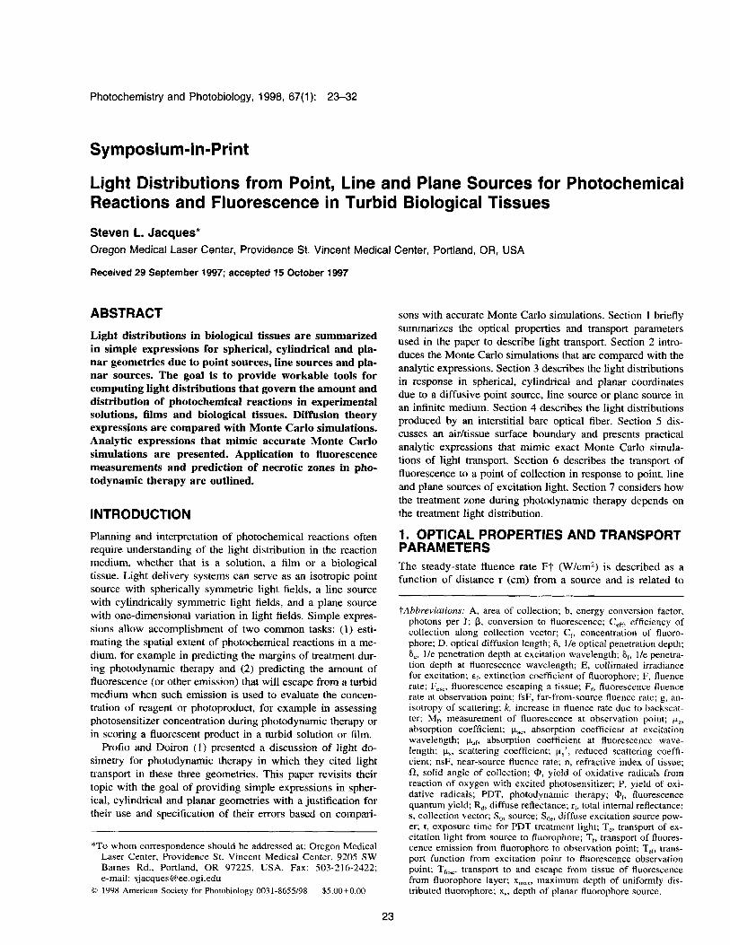
Figure 2 summarizes the results of the equations of section 3 that predict the form of F(r) for the three source geometries. Figure 3 shows the residual errors in the Auence rate predicted by diffusion theory, FD,, relative to the prediction of Monte Carlo, FMc: error = (FDT - FMC)/FMc. For a plane source in Figs. 2 and 3 and the following paragraph, F(r) denotes F(x).

One can consider the fluence rate in two regions: the near- source fluence rate (nsF) within the first 0.17 cm (r/6 < 1) and the far-from-source fluence rate (fsF) beyond 0.17 cm (r/6 > 1). In the nsF region, diffusion theory seriously underestimates the fluence rate. In the fsF region, diffusion theory is more accurate but still contains errors, and the ex- planation is given in the summary at the end of this section. The magnitude of nsF scales as spherical > cylindrical > planar. The rate of decline of fsF scales as spherical > cylindrical > planar. The spherical fluence rate initiates with the strongest magnitude but declines most rapidly, while the planar fluence rate intiates with the lowest magnitude but declines least rapidly. Hence, the magnitude of F initially scales as spherical > planar but crosses over at about 1 cm (r/6 = 5) to become planar > spherical. One can always adjust the power of a light source to modify the magnitude of F, but the spread of light depends on the tissue and source

Photochemistry and Photobiology, 1998, 67(1) 25

0.2 plane source

-0.8.

-1-- :

1'

1 J.

: : : ; : : : : ; : : : : ; : : : : ,

line source

1 0 ' _,___ plane t

poinS7

0 0.5 1 1.5 2 2.5 3

0 .1 ; : ; : ; : ; : ; : ; : F 0 0.05 0.1 0.15 0.2 0.25 0.3

r [cml

Figure 2. Fluence rate distribution F(r) (W/cm2) in response to a diffusive source, either a point source So (W), a line source So (W/cm) or a plane source So (W/cm2) in an infinite medium with no boundaries. The y axis presents the fluence rate normalized by the source, F(r)/So. For plane source, F(r) denotes F(x). (Upper) Over 3 cm radial distance from source. (Lower) Over 3 mm distance. The dashed lines are diffusion theory and the solid lines are Monte Carlo. The optical properties in all figures of this paper are pa = 1 cm-', ks = 100 cm-' and g = 0 such that pb' = 10 em- \ and 6 = 0.174 cm.

geometry that motivates the use of the equations of this section.

Any practical light delivery device will have a finite volume and assert a boundary condition at the device/tissue interface that will dominate the nsF. For example, a spherical diffuser tip like that of Marijnissen and Star (5) or the cylindrical diffuser fibers commercially available for photodynamic therapy (PDT) may have a radius of 0.5-1 mm. Such devices, when placed interstitially in tissue, will seriously perturb the predicted nsF, slightly perturb the fsF close to the device and not significantly affect the fsF distant from the device. Hence, the equations of this section are of practical value in predicting tissue penetration by light delivered with common devices; however, they do not provide accurate descriptions of the fluence rate very close to a device. Profio and Doiron (1) considered the size of a device in their expressions for F(r).

Spherical geometry

When the diffusion equation is expressed in spherical coordinates, the solution is the spherical point spread function F(r) that includes the term exp(-r/6). To specify F(r) fully we can invoke conservation of energy. Consider a point source So (W). The total amount of energy deposition equals the integral over all space of the product paF(r), and this

-0. 4 i I N ' ' plane source line source point source

I . . . . I . . . . ~

0 0.05 0.1 0.15 0.2 0.25 0.3

r [cml Figure 3. Residual error in diffusion theory based on calculated fluence rate using diffusion theory (FDT) and Monte Carlo (FMc). The error is defined as (FDT - FM&FMc. Diffusion theory seriously underestimates fluence rate near the source. Errors are less at positions distant from the source. (Upper) Within 2 cm radial distance from source. (Lower) Within 3 mm distance.

total energy deposition must match the source energy. Con- servation of energy in spherical coordinates requires that

~ompaF(r)4nrzdr = So

where 4m2dr is the incremental volume (cm3) associated with an incremental spherical shell at r. If F(r) includes the term exp(-r/6), then the solution for F(r) that conserves energy is

S,exp( -r/6) 4.srp,,S2r

F(r) =

Note that to conserve energy in spherical coordinates a factor 1 / (4~p ,6~r ) was required. Equation 2 was used to generate the curves for a point source in Figs. 2 and 3.

Not shown but important to note is that Monte Carlo simulations were conducted twice, once with the g = 0 denoting isotropic scattering and again with g equal to 0.90 denoting forward-directed scattering typical of tissues. The wS' was held constant at 10 cm-I in both cases. The two curves are indistinguishable in the graph, illustrating the concept of the similarity relation which holds that the choice ps', rather than the choices of ps and g, specifies F(r). The similarity relation holds when the ratio ps'/pa exceeds 10 such that many scattering events occur before a photon is likely to be absorbed. In the region near the source, the similarity relation also requires that g is high such that Ups << Ups'.


Cylindrical geometry

When the diffusion equation is expressed in cylindrical coordinates, the solutions are Bessel functions. The particular Bessel function that yields the appropriate real (not mathe- matically imaginary) solution is the function K, called the modified Bessel function of the first kind. The function can be ap roximated by the proportionality Ko(u) - = r/6 for the diffusion problem. Star (eq. 6.113, p. 178 in chapter 6 of Welch and van Gemert (7)) specified the constant of proportionality to be 3(pa + pS')/27r such that the asymptotic form of F(r) at large r is

exp(-u) .,re d 2 u for large u (p. 397 in Butkov (6)), where u

Let us derive our own formula by following the same energy conservation logic applied above to the spherical geometry. Conservation of energy in cylindrical coordinates requires that

8' kL,F(r)2rr dr = So (4)

where 27rr dr is the incremental volume per unit length (cm3/ cm) associated with an incremental cylindrical shell at r. If the form of F[r) is &[r/6), then the solution for F(r) that conserves energy is

A line source is equivalent to a line of point sources. For comparison, let us compute a numerical solution to the cylindrical problem based on the spherical point spread function, Eq. 2, here denoted as Fsph(r), Consider an infinite line source So (W/cm) that extends along the z axis (see Fig. 1). The r axis is perpendicular to the z axis. An observation point (z = 0, r) is located at a distance R = from an incremental portion of the line source at position (2, r = 0). Integrating the contributions from all incremental por- tions of the line source to the particular observation point yields:

(6)

The integration was accomplished numerically using Math- ematicam and the result is identical to the result in Eq. 5 that was used to generate the curves for a line source in Figs. 2 and 3.

The asymptotic expression, Eq. 3, is simple and convenient, whereas Eq. 5 requires access to a subroutine to im- plement &, often available but not on every calculator or spread sheet. Figure 4 plots the residual error of the asymptotic expression relative to the predictions of Monte Carlo: error = (Fa,, - FMc)/FMc. For comparison, the error of Eq. 5 is again shown. The asymptotic expression has more error near the source than Eq. 5 but they share similar error at larger r. At large r, the asymptotic expression is a useful tool.

-0. etl t

for line source : : : : : : : : : ,

0 0.2 0.4 0.6 0.8 1 r [cml

Figure 4. Residual error in the asymptotic diffusion theory expression for fluence rate due to a line source, Eq. 3 by Star (7). Error expressed as (Fasy - F M c ) / F M c . For comparison, the residual error for the expression using the Bessel function KO, Eq. 5 , is also shown. The asymptotic expression is a more simple and convenient expression than Eq. 5 and is appropriate at larger r.

Planar geometry

When the diffusion equation is expressed in planar coordinates, the solution F(x) has the form exp( -r/S). Conservation of energy in planar coordinates in response to an infinitely broad planar source So (W/cm2) requires that

Jl I*aF(X) dx so (7)

where dx is the incremental volume per unit area (cm3/cm2) associated with an incremental planar layer at x. If the form of F(x) is exp(-x/8), then the solution for F(x) that conserves energy is

Soexp( ~ x/6) F(x) = 2FaS .

It should be emphasized that Eqs. 7 and 8 refer to an ideal diffusive planar source that propagates in the Itx directions. A typical example is a thin planar layer of fluorophore within a turbid medium that radiates fluorescent emission when uniformly excited.

A plane source is equivalent to a plane of point sources. For comparison, let us compute a numerical solution to the planar problem based on the spherical point spread function, Eq. 2, here denoted as Fsph(r). Consider an infinite line source S , (W/cm2) that extends in the y-z plane. An observation point (x, y = 0, z = 0) is located at a distance R = d x 2 + y2 + z2 from an incremental area on the plane source at position (x = 0, y, z). Integrating the contributions from all incremental areas on the plane source to the particular observation point yields:

F(x) = I: Fsph(R) dy dz (9)

The integration was accomplished numerically using Math- ematica. The numerical result exactly matches the energy conserving F(x), Eq. 8.

Summary

The diffusion theory expressions for fluence rate as a function of distance from a point source, line source and plane source in an infinite homogeneous medium are given by Eqs.


5. BOUNDARY CONDITIONS: AN AIIUTISSUE SURFACE When there is an air/tissue surface boundary two compli- cations arise: (1) significant total internal reflection of light at the boundary affects the light distribution, and (2) the escape of light at the boundary is significant. This section considers practical and accurate descriptions of light distributions in the presence of a surface boundary.

Figure 5. Bare fiber placed interstitially within tissue launches light forward, then diffusion appears to be centered from a position 1 mfp’ = l/(bd + JL,’) or about 1 mm in front of fiber.

2, 5 and 8, respectively. Far from a line source, the asymptotic expression Eq. 3 is as accurate and more convenient than Eq. 5.

Diffusion theory fails near sources where the gradients of fluence rate are changing so quickly that they are not linear within a region of a few diffusion lengths in size. Just because a diffusion theory expression for F(r) conserves energy does not mean that it is the correct F(r). The errors near the source are incorporated in the integration to conserve energy and hence the above expressions are necessarily wrong. The error that occurs near the source forces an error distant from the source, and indeed Fig. 3 shows residual errors far from the source. Diffusion theory can predict the general shape of F(r) but its prediction of the absolute value of F(r) is suspect due to the above error. With this caveat, diffusion theory is a useful tool in planning light distributions for photochemical reactions far from a source.

4. INTERSTITIAL BARE FIBER A special case of interest is a bare optical fiber placed in- terstially in a tissue. The photons exit the fiber in one direction and hence the fiber is not an isotropic source. However, the “center of mass” of photons that are launched forward by a fiber appears to be located at a position, which is one transport mean free path, mfp’ = l/(pa + p,’), from the tip of the fiber, as illustrated in Fig. 5. Patterson et al. (8) used a point source placed one mfp’ below the aidtissue surface to simulate a narrow collimated beam of light orthogonally irradiating a tissue surface. Wang and coworkers (9,lO) have utilized this phenomenon for measuring optical properties by comparing the shift of the center of mass of photons launched by oblique versus orthogonal irradiation of a tissue surface by a narrow laser beam or optical fiber.

For our example of pa = 1 cm-’ and IJ.,‘ = 10 cm-I, the mfp’ equals 0.091 cm, about 1 mm. In the region near the fiber and near the center of mass, one uses Monte Carlo simulations to accurately predict the nsF. More commonly one is interested in the fsF where diffusion theory can reasonably predict the zone of treatment in PDT or the volume of some other photochemical reaction. By setting the origin (r = O j at one mfp‘ in front of the fiber, the spherical diffusion theory of Eq. 2 can be used to predict the light distribution fsF.

Surface boundary causes image source

An airkissue surface will cause roughly 50% of the light flux reaching the surface to be returned into the tissue by total internal reflection. When a photon attempts to exit a tissue or liquid medium into the air at too oblique an angle, the photon is reflected back into the medium. About half of diffusely reflected light is sufficiently oblique in approaching the surface to be internally reflected.

It is common in engineering to treat a reflective boundary by the method of images. One treats the semi-infinite tissue problem, with an airkissue surface and an imbedded source within the tissue, as an infinite tissue problem with both the original source and an additional image source located sym- metrically opposite the original source relative to the surface plane. The image source is assigned a negative value equal to the original positive source of light within the tissue. The gradient between these positive and negative sources in an infinite tissue problem mimics the flux of light from the original source out into the air in the semi-infinite tissue problem. Let the aidtissue surface reside in the y-z plane at x = 0. The method of images for an isotropic point source of strength So at a depth x, within a tissue, i.e. at position (xF, y = 0, z = 0), is summarized:

where

r = Vx2 + y2 + z2

r , = V(x - xs>2 + y2 + z*

r2 = d ( x + xs)2 + y2 + z*

where r l is the distance from the original source to an observation point at (x, y. z) and r, is the distance from the image source to the observation point. The negative term in the brackets is the contribution from the image source. The above Eq. 10 illustrates the method of images for an isotropic point source, but one can also use the method of images to treat imbedded cylindrical and planar sources near an air/ tissue surface boundary. Equation 10 is a very simple form of the method of images and provides a first approximation to the effects of an aidtissue surface boundary. Others have considered more exact treatments of the surface boundary condition. Farrel et al. (1 1) have outlined the method of images for the case of a collimated light source, a laser beam or optical fiber, orthogonally irradiating a tissue surface and show that the plane of symmetry is best placed slightly outside the true tissue surface in this case. Haskell et al. (12) discuss boundary conditions in detail citing references to previous work.


Table 1. nmrdium/nnr. at the surface boundary*

Empirical expression for how the six parameters of Eqs. 14 and 20 depend on diffuse reflectance R, for two refractive mismatches,

Parameter ntlssur/nalr = 1.38 nwatcJnatr = 1.33

3.09 + 5.44Rd - 2.12 exp(-21.5Rd)

2.09 - 1.45Rd - 2.09 exp(-21.5Rd) 1.53 exp(3.4Rd) 0.28 + 0.78Rd - 0.14 exp(-10.7Rd) 1 - 0.3 exp(-6.12Rd)

1 - 0.423 eXp(-20.1Rd) 3.04 + 4.09Rd - 2.06 exp(-21.1Rd) 1 - 0.423 exp(- 1 8.9Rd) 2.04 - 1.33Rd - 2.04 exp(-21.1Rd) 1.49 exp(3.36Rd) 0.32 + 0.72Rd - 0.16 exp(-9.11Rd) 1 - 0.30 exp(-6.12Rd)

Erratum: The expression for Cz for n = 1.38 corrects an error in Gardner ef al. (17).

Surface boundary effects in planar geometry

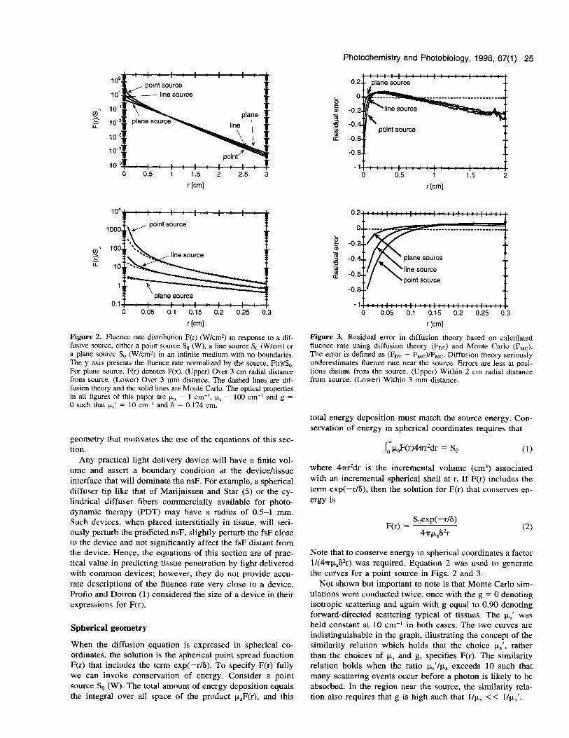
Devices used interstitially such as a bare fiber, an isotropic point source or a cylindrical diffuser fiber usually have an aidtissue boundary very distant from the source. However, topical irradiance of a tissue with a broad beam of light is a common situation and involves an airitissue boundary exactly at the plane source of light. For the planar case with a collimated light source irradiating an aidtissue surface, simple exponential expressions can correct diffusion theory (Eq. 8) to match Monte Carlo simulations.

Jacques (13) described planar light transport in simple terms:

(1 1)

where k is a constant that depends on the amount of total diffuse reflectance, R,, from the tissue and on the refractive mismatch at the air/tissue surface:

F(x) = S& exp(-x/6)

k = 3 + 5.1Rd - 2 exp(-9.7Rd) (12) which was based on Monte Carlo simulations using a broad range of optical properties to yield a range of & values. The value of R, depends on both the optical properties and the refractive mismatch at the tissue surface boundary. Jacques (14) used the accurate predictions of the adding4oubling method of Prahl (15,16) to develop an approximation for Rd:

R, = exp(-7.86pa) = exp(-7.8/v1 + ps'/pa) (13)

7 : : : : : : : : : : : : : : 6 - ' s

5.

4 -

3.

2 -

1 -

. for planar collimated irradiance at air/tissue surface

01 : : : : : : : : : : : : : : I 0 0.5 1 1.5

Depth, x [cm]

Figure 6. Planar light distribution in response to a broad collimated source orthogonally irradiating an aidtissue surface. The fluence rate, F(x) (W/cm*), is normalized by the collimated irradiance, So (W/cm*), to yield F(x)/S, (dimensionless), and is plotted versus depth in the tissue, x (cm). The upper curve is Eq. 11, k exp(-x/6), which predicts deep light penetration but overestimates the fluence rate at the surface. The lower curve is Eq. 14 that mimics Monte Carlo simulations. (F, = 0.1 cm-I).

which is essentially a statement of Beer's Law for transmis- sion through an apparent average photon pathlength of 7.86. The second expression on the far right illustrates that R, depends on the ratio pL,'/pa. The value 7.8 is appropriate for a refractive mismatch of tissue/air equal to 1.37 that is typical for a tissue with -80% water content. The above expression is reasonably accurate (error& < 5 % ) for 0.10 5 R, 5 0.60 and is independent of the scattering anisotropy, g, in the range 0.90 5 g 5 0.98. Outside these ranges of Rd and g, and for other refractive index mismatches, the factor 7.8 is not optimally accurate and should be adjusted.

Gardner et al. (17) included an additional exponential term to match not only the deeply penetrating light but also the superficial light distribution near the surface. The following analytic expression mimics the behavior specified by Monte Carlo simulations:

F(x) = So[Clexp(-k,x/6) - C,exp(-k2x/6)] (14)

where the factors C,, C2, k , , k2 are listed in Table 1 for refractive index mismatches of 1.38 (tissue with -70% water content) and 1.33 (water).

Figure 6 shows the behavior of Eqs. 11 and 14. In this figure, the absorption coefficient is 0.1 cm-I. The value of k in Eq. 11 would be 6.25 for a tissue with 1.37 refractive index, but to compare with Gardner's expression for a tissue with 1.38 refractive index, the value k has been adjusted to 6.57. Gardner's expression also accounts for the specular reflectance at that airkissue surface that slightly diminishes the incident light that enters the tissue. The deep light penetration behaves as a simple decaying exponential with an apparent surface plane source of 6.57S0. The delivered irradiance, So, is augmented by a factor of 6.57 due to the diffusely backscattered light that reaches the surface and the total internal reflection of light at the aidtissue interface. The Gardner prediction, Eq. 14, mimics accurate Monte Carlo simulations and illustrates how escaping reflectance causes a depletion of fluence rate near the surface.

6. FLUORESCENCE A measurement of fluorescence involves a source of excitation, So,, the transport of the excitation light from the source at r = 0 to fluorophores at r', T,(O + r'), the conversion to fluorescence at r', p(r'), and the transport of fluorescence to some point of observation a distance r = (0 -+ r) from the source at position r, Tf(r' + r). Figure 7 illustrates the geometry of fluorescence excitation and observation. The bold 0, r and r' are positions denoted as vectors


excitation f I uorescence source at 0 collection at r

0 r = (O-+r) r 1 b

r ’ fluorophore at r’

Figure 7. Observing fluorescence at position r due to a fluorophore at r’ in response to an excitation source at the origin 0. The distance from source to observation point is r = (0 + r). The distance from source to fluorophore is (0 -+ r’). The distance from fluorophore to observation point is (r’ + r).

and 0 -+ r’ and r’ -+ r denote distances between positions. Regardless of the geometry, the fluorescence fluence rate at a distance r from a source, FXr) (W/cm2), can be generically expressed:

FAr) = S,, I, T,(O -+ r‘)p(r’)T,(r’ -+ r) dV (15)

which is a volume integral over the tissue volume in which light penetrates and fluorophore resides. The term dV denotes the incremental volume at position r’ (dV = 47~r’~dr’ [cm3] in spherical coordinates, 2m’dr’ [cm2] in cylindrical coordinates and dr’ [cm] in planar coordinates). In general, the transport factor T equals F/S, and therefore has units of cm-? in spherical, cm-I in cylindrical, and dimensionless in planar coordinates. The transport factor T can be expressed as T, for transport of the excitation source and T, for transport of fluorescence emission. The conversion factor p equals the product qC@, where Ef is the fluorophore extinction coefficient (cm-’[mol ~ m - ~ ] - l ) , C, is the fluorophore concentration (mol cm-’) and @, is the fluorescence quantum yield with units W fluorescence emission per W absorbed excitation or dimensionless. Therefore, p has units of cm-’ and in general P(r’) can vary with location. The above treatment of fluorescence generation and transport in tissues has been presented by others, for example, for the steady-state by Keijzer et al. (1 S), in the time and frequency domains by Patterson and Pogue (19) and Hutchinson et al. (20).

The details of how a collection device samples the local fluence rate F,(r) (W/cm2) depend on how incremental flux dJ (W/cm2) enters the device through some incremental area of collection, dA (cm?), and incremental solid angle of collection, dQ (sr), driven by the local fluence gradient, VF (W/cm’)), along a unit collection vector s (dimensionless) that is centrally aligned with dfl, which is denoted VF.s. Usually a collection device, e.g. an optical fiber or a detector viewing a small aperture, will have a collection efficiency, C,&) (sr I ) that varies with the direction of collection. A measurement, Mf (W), of fluorescence can be described by the integral:

(16) Mf = f,J, -DfVF.sC,,,(s) dQ dA

where Df (cm) is the diffusion length for the wavelength of fluoresence and VF.s is a function of the position of dA, r. The negative sign indicates that flux moves down the fluence gradient. Beyond the generic Eq. 16, we will not discuss the details of collection by particular devices.

For the special case of a homogenous tissue with uniformly distributed fluorophore, p is a constant and Eq. 15 can be simplified:

F, = S,,P f, T,(O -+ r’)TXr’ -+ r) dV = S0,pT,, (17)

where T,, equals the volume integral of the product (penetration of the excitation source)(escape of the fluorescence). Tef has units of cm-2 in spherical coordinates, cm-I in cylindrical coordinates, and dimensionless in planar coordinates. In other words, all the information regarding tissue optics is incorporated in the single parameter TeF All the information regarding the fluorophore is in the parameter p.

Spherical geometry

Consider a point source of excitation at the origin 0 in an infinite homogeneous tissue with uniformly distributed fluorophore and a collection point r for observing fluorescence at a distance r = (0 -+ r) from the source. In spherical coordinates, the expression for Tef(r) was derived (S.L. Jacques, J.-M. Tualle and S. Avrillier, Univ. of Paris, XIII, personal communication):

exp[-(0 -+ r’)/S,]exp[-(r’ r)/Sf] 4np,,S:(O -+ r’) 41~p,,6f(r‘ + r)

d’r’ Tedr) =

where pa, and par are the absorption coefficients and 6, and €+ are the l/e penetration depths at the wavelengths for excitation and fluorescence as denoted by the subscripts e and f. This expression can be used with Eq. 17 to interpret measurements of fluorescence using interstitially placed excitation and collection fibers. If the fibers are sufficiently sepa- rated (p >> S,, p >> Sf), the expression is reasonably accurate.

Cylindrical geometry

Consider an infinite line source of excitation in an infinite homogeneous tissue with uniform fluorophore and the transport of fluorescence to an observation point at a distance r from the line source. A line source of excitation is equivalent to a line of excitation point sources. Analogous to how Eq. 6 used Eq. 2 to yield Eq. 5, Eq. 6 uses Eq. 18 to calculate the integration of the spherical T,, along an infinite line source that yields the cylindrical Tef:

A common example is the observation of photosensitizer fluorescence by a point collector in response to excitation by the PDT treatment light delivered by a cylindrical diffusive optical fiber. The point collector can be an isotropic optical fiber collector like that of Marijnissen and Star (5) or a bare fiber collecting from a position one mfp’ in front of the fiber. The point collector should be located near the


middle of the cylindrical fiber so that the fiber appears infinite in length from the perspective of the collector.

Planar geometry

Consider an infinite plane source of excitation in an infinite homogeneous tissue with uniform fluorophore and the transport of fluorescence to an observation point at a distance x from the plane source. A plane source of excitation is equivalent to a plane of excitation point sources. Analogous to how Eq. 9 used Eq. 2 to yield Eq. 8, Eq. 9 uses Eq. 18 to calculate the integration of the spherical Tef over an infinite plane source that yields the planar Tef:

A common example for this planar geometry in an infinite scattering medium is not obvious. The situation would in- volve a diffusive plane source of excitation at x = 0 and observation of fluorescence by a point collector a distance x from the plane source.

Planar collimated excitation at aidtissue surface

A broad uniform beam of collimated excitation light irradiating an air/tissue surface to excite fluorescence in a homogeneous medium is a common problem. First, let us consider how to adapt diffusion theory to treat this problem. Then, we shall compare the results with the Gardner equations that mimic Monte Carlo simulations.

First, consider the penetration of excitation light. The diffusion theory expression Eq. 8 has the proper exponential form but not the correct absolute value. However, Eq. 12 based on Monte Carlo simulations specifies the factor k which enables Eq. 11 to accurately describe the deep penetration of excitation light to a planar layer of fluorophore at a depth x, in response to a collimated excitation irradiance E (W/cm’):

F, = Ekexp(-xs/S,) (21)

The transport of excitation is T, = F, / E which equals:

T, = kexp( -x,/S,) (22)

Second, consider the transport of fluorescence to the tissue surface and its escape from the tissue for observation. Equa- tion 8 can directly describe the transport of fluorescence from x, to the surface. To account for the influence of the surface boundary, consider a simple two-flux model sche- matically shown in Fig. 8. The outward flux of flourescence along the x axis is called J. Total internal reflectance creates an inward flux I = r,J where r, = 0.668 + 0.0636n + 0.710/n - 1 .440/n2. The measurable escaping flux of fluorescence is F,,, = (1 - rJJ. The total fluence rate within the tissue at the surface is Ff = 2(1 + J), where the factor 2 accounts for the average zig-zag path L of diffuse photons as flux moves in the t x directions such that AL/Ax = 2. Substituting for I and J using I = J/r, and J = F,,J(l - rJ yields Ff = 2F,,,(1 + r,)/(l - rJ. Therefore, F,,, = FX1 - r,)/[2(1 + rJ]. The transport of fluorescence to the surface including its escape out of the tissue for observation is expressed Tfesc = Ffe,,/Sof (dimensionless), which equals:

air

~~

f I u o roph o re -I a y & Figure 8. Schematic of two-flux model for how air/tissue surface affects fluorescence near surface. Diffuse flux toward surface (J) from deep fluorescent layer is reflected by total internal reflectance (r,) to yield diffuse flux from surface (I). Escaping fluorescence (FCJ is observable by measurement. On average, diffuse photons move a pathlength AL that is twice the net movement Ax along the x axis to or from the surface: AL = 2Ax.

In summary, the observable flux of escaping fluence, F,,, (W/cm2), from a fluorophore layer at x, in response to an excitation irradiance E (W/cm2) is approximately:

(24) Now consider the equations that Gardner et al. (17,21)

used to mimic accurate Monte Carlo simulations of T, and TfeSc. The transport of excitation, T,, is described by Eq. 14 appropriately using pae and 6,. This equation already considers the effects of specular reflectance and total internal reflectance. The transport and escape of fluorescence, Tfe,,, from a planar source at depth x, was modeled by Monte Carlo simulations and mimicked by a simple exponential expression by Gardner et al.:

where C3 and k3 are specified in Table 1. This expression describes the fluorescence that successfully escapes the tissue for observation and therefore includes the effects of total internal reflectance at the aidtissue boundary.

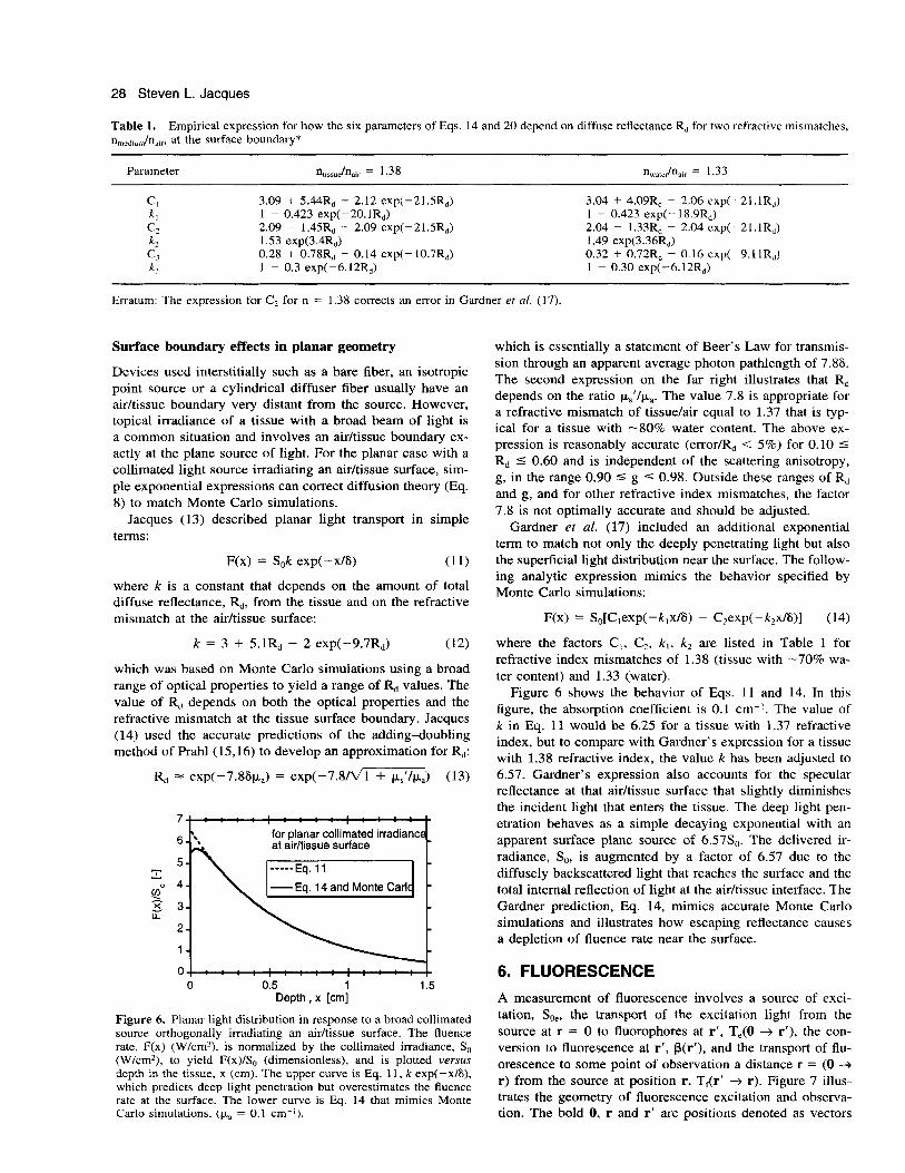
In Fig. 9, the factors T,, Tfesc and the product TeTfesc are plotted versus the depth x, where the incremental fluorophore layer resides. Near the surface, diffusion theory (dashed lines) and the Gardner equations (solid lines) that mimic Monte Carlo disagree for T,, agree for Tfesc and disagree for TeTfesc. Diffusion theory overestimates the amount of observable fluorescence expected from a superficial fluorophore layer. The error derives from the error in T, because a diffuse source poorly models the collimated excitation. The lack of error in Tfesc suggests that the simple two-flux treatment of the boundary condition is adequate for a deep dif-


r! 'ti 0

m "-

-mimic Monte Carlo .-

0 0.1 0.2 0.3 0.4 0.5 0.6 Depth of fluorophore layer, xs [cm]

Figure 9. Planar transport of excitation (T,) to a fluorophore layer at depth x,, transport of fluorescence (TfeJ from the fluorophore layer to the surface including its escape from the tissue and the product T,Tr,,,, as functions of x, (cm). Dashed lines are diffusion theory (Eqs. 22, 23) and solid lines are equations that mimic Monte Carlo simulations (Eqs. 14, 25, Table 1 for n = 1.38).

fuse source. Diffusion theory begins to overestimate Tfesc as p,, decreases below 1 cm-I. For deeper x, beyond 1 mm, diffusion theory and the Gardner equations agree. The conclusion is that diffusion theory accurately predicts the escaping fluorescence due to an isolated deep fluorophore layer but yields significant error when applied to superficial fluorophore layers. Measurement of uniformly distributed fluorophores will be dominated by the errors due to superficial fluorophores. Optical properties are the same for excitation and fluorescence wavelengths, the same as in Fig. 2.

To predict the fluorescence from a tissue with uniformly distributed fluorophore, let us return to the Gardner equations that mimic Monte Carlo simulations. One calculates T,, by substituting Eqs. 14 and 25 into Eq. 17:

where fluorophore is uniformly distributed from the surface to a depth xmaX. When x,,, is so deep that negligible fluorescence escapes from that depth, x,,,, may be assigned the value infinity and the above expression simplifies:

The above equation accurately describes the total escaping fluorescence from a homogeneous tissue with uniform fluorophore that is irradiated with collimated excitation at its surface. Tissue surface roughness may cause the observed fluorescence to deviate slightly from this prediction.

7. PHOTODYNAMIC THERAPY A practical use of diffusion theory is to predict the extent of treatment during PDT (22). Consider a planar irradiance and the simple Eq. 1 1 to describe planar light transport. The yield of oxidative radicals as a function of depth, P(x) (mol- eculeslcm'), is described:

P(x) = S,tbeC@kexp( -x/6) (28)

where So is the irradiance, t is the exposure time (s), E and C are the extinction coefficient and concentration of the photosensitizer and the product EC has units of cm-I, b is the energy conversion factor (photons per J) at a given wavelength, @ is the yield of oxidative radicals from the reaction of oxygen with excited photosensitizer (dimensionless) (oxygen dependence has been lumped into this parameter for simplicity) and kexp( -XIS) is the light penetration of Eq. 1 1. A light exposure induces a necrotic zone that extends to a depth z,,,,,,,, where a threshold toxic amount of oxidative radicals has been produced, Pth. Substituting xnecrorlc for x and Pth for P ( X , , , ~ ~ ~ ~ , ~ ) , one can solve for the depth of necrosis:

The above equation illustrates that the necrotic zone is directly proportional to the optical penetration S but proportional to the natural logarithm of all other parameters. To double xnecmsis, one need only double 6 but must increase any other parameter (or decrease Pth) by a factor of 7.4.

CONCLUSION In conclusion, this paper has presented simple expressions for steady-state light transport due to point, line and plane sources and illustrated how they pertain to fluorescence measurements and PDT. The analysis can be extended to the time-dependent case expressed either in the time domain or the frequency domain. This paper has not addressed how to measure optical properties in order to use the equations of this paper.

A major conclusion of this paper is that the shape of the fluence rate distributions due to point, line, and plane sources are accurately described by the cited diffusion theory equations, however the absolute values of the fluence rates are poorly predicted. The use of Monte Carlo simulations to provide accurate correction factors to the diffusion theory expressions is reported for a planar source and future work should document the corrections for point and line sources as well.

Acknowledgements-This work was supported by the National In- stitutes of Health (R29 HL45045) and the Department of Energy (DE-FG03-97ER62346).

REFERENCES 1. Profio, A. E. and D. R. Doiron (1987) Transport of light in tissue

in photodynamic therapy. Photochenr Photobiol. 46, 59 1-599. 2. Wang, L.-H., S . L. Jacques and L.-Q. Zheng (1995) MCML-

Monte Carlo modeling of photon transport in multi-layered tissues. Comput. Methods Prog. Biomed. 47, 13 1-1 46.

3. Jacques, S. L. and L. Wang (1995) Monte Carlo modeling of light transport in tissues. In Optical-Thermal Response of laser- Irradiated Tissue (edited by A. J. Welch and M. J. C. van Gem- ert). Plenum Press, New York.

4. Software for various Monte Carlo simulations including the pro- gram used for this paper is available on the Internet: http:// ee.ogi.edu/-sjacques/rnontecarlo.html.

5. Marijnissen, J. P. and W. M. Star (1996) Calibration of isotropic light dosimetry probes based on scattering bulbs in clear media. Phys. Med. Biol. 41, 1191-1208.

6. Butkov, E. ( 1 968) Mathematical Physics. Addison-Wesley, Reading, MA.

7. Star, W. M. (1995) Diffusion theory of light transport. In Op-


tical-Thermal Response of Laser-Irradiated Tissue (edited by A. J. Welch and M. J. C. van Gemert). Plenum Press, New York.

8. Patterson, M. S., B. Chance and B. C. Wilson (1989) Time resolved reflectance and transmittance for the noninvasive measurement of tissue optical properties. Appl. Opt. 28,233 1-2336.

9. Wang, L.-H. and S. L. Jacques (1995) Use of a laser beam with an oblique angle of incidence to measure the reduced scattering coefficient of a turbid medium. Appl. Opt. 34, 2362-2366.

10. Lin, S.-P., L.-H. Wang, S . L. Jacques and F. K. Tittel (1997) Measurement of tissue optical properties using oblique incidence optical fiber reflectometry. Appl. Opt. 36, 136-143.

1 1 . Farrel, T. J., M. S . Patterson and B. Wilson (1992) A diffusion theory model of spatially resolved, stead-state diffuse reflectance for the noninvasive determination of tissue optical properties in viva. Med. Phys. 19, 881-888.

12. Haskell, R. C., L. 0. Svaasand, T.-T. Tsay, T.-C Feng, M. S . McAdams and B. J. Tromberg (1994) Boundary conditions for the diffusion equation in radiative transfer. J. Opt. SOC. Am. A 11, 2727-2741.

13. Jacques, S. L. (1989) Simple theory, measurements, and rules of thumb for dosimetry during photodynamic therapy. In Pho- todynamic Therapy: Mechanisms, Vol. 1065 (Edited by T. J. Dougherty), pp. 100-108. Proc. SPIE.

14. Jacques, S . L. (1996) Reflectance spectroscopy with optical fiber devices and transcutaneous bilirubinometers. In Biomedical Op- tical Insfrumentation and Laser-Assisted L?iotechnology, NATO

ASA Series (Edited by A. M. Verga Scheggi et al.). Kluwer Academic, Dordrecht, Netherlands.

15. Prahl, S . A., M. J. C. van Gemert and A. J. Welch (1993) De- termining the optical properties of turbid media by using the adding-doubling method. Appl. Opt. 32, 559-569.

16. Prahl, S. A. (1995) The adding-doubling method. In Optical- Thermal Response of Laser-Irradiated Tissue (Edited by A. J. Welch and M. J. C. van Gemert). Plenum Press, New York.

17. Gardner, C. M., S. L. Jacques and A. J. Welch (1996) Light transport in tissue: accurate expressions for one-dimensional fluence rate and escape function based upon Monte Carlo simulation. Laser Surg. Med. 18, 129-138.

18. Keijzer, M., R. Richards-Kortum, S . L. Jacques and M. S. Feld ( 1 989) Fluorescence spectroscopy of turbid media: autofluores- cence of the human aorta. Appl. Opt. 28, 42864292.

19. Patterson, M. S. and B. W. Pogue (1994) Mathematical model for time-resolved and frequency-domain fluorescence spectroscopy in biological tissues. Appl. Opt. 33, 1963-1974.

20. Hutchinson, C. L., T. L. Troy and E. M. Sevick-Muraca (1996) Fluorescence-lifetime determination in tissues and other random media from measurement of excitation and emission kinetics.

21. Gardner, C. M., S. L. Jacques and A. J. Welch (1996) Fluores- cence spectroscopy of tissue: recovery of intrinsic fluorescence from measured fluorescence. Appl. Opt. 35, 1780-1792.

22. Jacques, S. L. (1992) Laser-tissue interactions: photochemical, photothermal, and photomechanical. Surg. Clin. North Am. 72, 531-558.

Appl. Opt. 35, 2325-2332.

light distributions from point, line and plane sources for ... and photobiology, 1998, 67(1): 23-32...

Documents