linear systems with markov jumps and multiplicative … · barbieri, fabio linear systems with...
TRANSCRIPT

FABIO BARBIERI
LINEAR SYSTEMS WITH MARKOV JUMPS ANDMULTIPLICATIVE NOISES - THE CONSTRAINED TOTAL
VARIANCE PROBLEM
Submitted in partial fulfillment for the degreeof Master in Science to the Escola Politéc-nica of Universidade de São Paulo.
São Paulo2016

FABIO BARBIERI
LINEAR SYSTEMS WITH MARKOV JUMPS ANDMULTIPLICATIVE NOISES - THE CONSTRAINED TOTAL
VARIANCE PROBLEM
Submitted in partial fulfillment for the degreeof Master in Science to the Escola Politéc-nica of Universidade de São Paulo.
Concentration field:
Systems Engineering
Advisor:
Prof. Dr. Oswaldo Luiz do Valle Costa
São Paulo2016

Catalogação-na-publicação
Barbieri, Fabio Linear systems with Markov jumps and multiplicative noises - Theconstrained total variance problem / F. Barbieri -- São Paulo, 2016. 103 p.
Dissertação (Mestrado) - Escola Politécnica da Universidade de SãoPaulo. Departamento de Engenharia de Telecomunicações e Controle.
1.Controle estocástico 2.Sistemas lineares 3.Controle ótimo 4.Variânciamáxima 5.Otimização de carteira de investimentos I.Universidade de SãoPaulo. Escola Politécnica. Departamento de Engenharia de Telecomunicaçõese Controle II.t.

ACKNOWLEDGEMENT
I thank all the people who contributed to this work with reviews and suggestionsthat made it fairly less confusing and complicated.
I am thankful to prof. Celma de Oliveira Ribeiro, prof. Alexandre Oliveira, prof.Antonio H. P. Selvatici, and André M. de Oliveira for spending so much time carefullyreading my work and pointing out my mistakes and how to improve the overall quality.
I express my gratitude to prof. Christian Heyerdahl-Larsen and prof. Jeff Skinnerfor recommending me to the program.
I am grateful to prof. Oswaldo L. V. Costa for his generosity by accepting me asone of his advisee, for his guidance on how to enhance my work, and for hanging ondespite the long time I take to learn anything.
I thank prof. Antonio Marcos Botelho for helping me by checking the mathematicalproofs and for his immense patience, generosity, and friendship over so many years.

RESUMO
Neste trabalho, estudamos o problema do controle ótimo estocástico de sistemaslineares em tempo discreto sujeitos a saltos Markovianos e ruídos multiplicativos. Con-sideramos a otimização multiperíodo, com horizonte de tempo finito, de um funcionalda média-variância sob um novo critério. Neste novo problema, maximizamos o valoresperado da saída do sistema ao mesmo tempo em que limitamos a sua variânciatotal ponderada pelo seu parâmetro de risco. A lei de controle ótima é obtida atravésde um conjunto de equações de diferenças de Riccati interconectadas, estendendo re-sultados anteriores da literatura. São apresentadas simulações numéricas para umacarteira de investimentos com ações e um ativo de risco para exemplificarmos a apli-cação de nossos resultados.
Palavras-chave: Controle estocástico. Sistemas lineares. Controle ótimo. Variân-cia máxima. Otimização de carteiras de investimento.

ABSTRACT
In this work we study the stochastic optimal control problem of discrete-time linearsystems subject to Markov jumps and multiplicative noises. We consider the multi-period and finite time horizon optimization of a mean-variance cost function under anew criterion. In this new problem, we apply a constraint on the total output varianceweighted by its risk parameter while maximizing the expected output. The optimalcontrol law is obtained from a set of interconnected Riccati difference equations, ex-tending previous results in the literature. The application of our results is exemplifiedby numerical simulations of a portfolio of stocks and a risk-free asset.
Keywords: Stochastic control. Linear systems. Optimal control. Maximum vari-ance. Portfolio optimization.

CONTENTS
List of Figures
List of Tables
1 Introduction 14
1.1 Objective . . . . . . . . . . . . . . . . . . . . . . . . . . . . . . . . . . . 14
1.2 Motivation . . . . . . . . . . . . . . . . . . . . . . . . . . . . . . . . . . . 14
1.3 Structure . . . . . . . . . . . . . . . . . . . . . . . . . . . . . . . . . . . 15
2 Literature review 16
2.1 Markov jumps and multiplicative noises . . . . . . . . . . . . . . . . . . 16
2.2 Solvability and well-posedness of indefinite stochastic systems . . . . . 18
2.3 The auxiliary problem . . . . . . . . . . . . . . . . . . . . . . . . . . . . 21
2.4 The introduction of risk parameters . . . . . . . . . . . . . . . . . . . . . 23
2.5 The state of the art and problem overview . . . . . . . . . . . . . . . . . 24
3 Portfolio management model 26
3.1 Brief historical overview . . . . . . . . . . . . . . . . . . . . . . . . . . . 26
3.2 Model formulation . . . . . . . . . . . . . . . . . . . . . . . . . . . . . . 27
3.3 PC(ν, β, α) problem overview under the portfolio management perspective 32
4 The optimal control of linear system with Markov jumps and multiplicative
noises 33
4.1 Notation and definitions . . . . . . . . . . . . . . . . . . . . . . . . . . . 33

4.2 The linear system with Markov jumps and multiplicative noises . . . . . 34
4.3 The constrained problem formulation, PC(ν, β, α) . . . . . . . . . . . . . 36
4.4 The unconstrained problem formulation, PU(ν, ξ) . . . . . . . . . . . . . 37
4.5 Mathematical operators . . . . . . . . . . . . . . . . . . . . . . . . . . . 38
4.6 Previous results . . . . . . . . . . . . . . . . . . . . . . . . . . . . . . . . 41
4.7 Optimal control law algorithm . . . . . . . . . . . . . . . . . . . . . . . . 43
5 Main results 45
6 Numerical examples 50
6.1 Input parameters estimation . . . . . . . . . . . . . . . . . . . . . . . . . 50
6.1.1 Data series . . . . . . . . . . . . . . . . . . . . . . . . . . . . . . 50
6.1.2 Market’s operation modes . . . . . . . . . . . . . . . . . . . . . . 51
6.1.3 Expected returns . . . . . . . . . . . . . . . . . . . . . . . . . . . 54
6.1.4 Expected covariances . . . . . . . . . . . . . . . . . . . . . . . . 55
6.2 Simulations’ results . . . . . . . . . . . . . . . . . . . . . . . . . . . . . . 56
6.2.1 Simulations for different levels of α . . . . . . . . . . . . . . . . . 57
6.2.2 Sensitivity analysis for β and ν . . . . . . . . . . . . . . . . . . . 63
6.2.3 Sensitivity analysis summary and final comments . . . . . . . . . 69
7 Conclusion 70
Appendix A -- Demonstration of the vector formulation in Theorem 2 72
Appendix B -- Numerical data of simulations of Section 6.2.1 75
Appendix C -- Further sensitivity analysis of β and ν 79

C.1 Simulations for different constant levels of β and ν . . . . . . . . . . . . . 80
C.2 Simulations for different combinations of β and ν . . . . . . . . . . . . . 86
C.2.1 Sensitivity analysis when α is not applied . . . . . . . . . . . . . 89
C.2.2 Analysis for scenarios uc and dc . . . . . . . . . . . . . . . . . . 93
C.2.3 Analysis for scenarios cd and cu . . . . . . . . . . . . . . . . . . 95
C.2.4 Analysis for scenarios ud and dd . . . . . . . . . . . . . . . . . . 97
C.2.5 Analysis for scenarios uu and du . . . . . . . . . . . . . . . . . . 99
References 101

LIST OF FIGURES
1 Ibovespa index and its weekly average returns. . . . . . . . . . . . . . . 52
2 Ibovespa’s operation modes distributions. . . . . . . . . . . . . . . . . . 54
3 System’s output for all scenarios. . . . . . . . . . . . . . . . . . . . . . . 59
4 System’s output variance for all scenarios. . . . . . . . . . . . . . . . . . 60
5 Control policy for scenario A. . . . . . . . . . . . . . . . . . . . . . . . . 61
6 Control policy for scenario B. . . . . . . . . . . . . . . . . . . . . . . . . 61
7 Control policy for scenario C. . . . . . . . . . . . . . . . . . . . . . . . . 62
8 Control policy for scenario D. . . . . . . . . . . . . . . . . . . . . . . . . 62
9 System’s output for scenario COMBINED − 7, beta7, nu7, and base sce-
nario cc. . . . . . . . . . . . . . . . . . . . . . . . . . . . . . . . . . . . . 66
10 System’s output variance for scenario COMBINED − 7, beta7, nu7, and
base scenario cc. . . . . . . . . . . . . . . . . . . . . . . . . . . . . . . . 66
11 Control policy for scenario COMBINED − 7 versus the base scenario cc. 67
12 System’s output for scenario COMBINED-5,6,7,8,9 and base scenario cc. 68
13 System’s output variance for scenario COMBINED-5, 6, 7, 8, 9 and base
scenario cc. . . . . . . . . . . . . . . . . . . . . . . . . . . . . . . . . . . 68
14 Illustrative diagram for the scenarios of Table 20. . . . . . . . . . . . . . 81
15 System’s output when β and ν are constants. . . . . . . . . . . . . . . . 82
16 System’s output variance when β and ν are constants. . . . . . . . . . . 83
17 Control policy for scenario cc. . . . . . . . . . . . . . . . . . . . . . . . . 84
18 Control policy for scenario cc2. . . . . . . . . . . . . . . . . . . . . . . . 84
19 Control policy for scenario cc4. . . . . . . . . . . . . . . . . . . . . . . . 85

20 Control policy for scenario cc8. . . . . . . . . . . . . . . . . . . . . . . . 85
21 Illustrative diagram for the scenarios of Table 22. . . . . . . . . . . . . . 87
22 System’s output for the scenarios of Table 22. . . . . . . . . . . . . . . . 88
23 System’s output variance for the scenarios of Table 22. . . . . . . . . . . 88
24 System’s output for the scenarios of Table 23. . . . . . . . . . . . . . . . 90
25 Zoom of Figure 24. . . . . . . . . . . . . . . . . . . . . . . . . . . . . . . 90
26 System’s output variance for the scenarios of Table 23. . . . . . . . . . . 91
27 Zoom of Figure 26. . . . . . . . . . . . . . . . . . . . . . . . . . . . . . . 91
28 Zoom of Figure 27. . . . . . . . . . . . . . . . . . . . . . . . . . . . . . . 92
29 Control policy for scenario uc versus scenario cc. . . . . . . . . . . . . . 94
30 Control policy for scenario dc versus scenario cc. . . . . . . . . . . . . . 94
31 Control policy for scenario cd versus scenario cc. . . . . . . . . . . . . . 96
32 Control policy for scenario cu versus scenario cc. . . . . . . . . . . . . . 96
33 Control policy for scenario ud versus scenario cd. . . . . . . . . . . . . . 98
34 Control policy for scenario dd versus scenario cd. . . . . . . . . . . . . . 98
35 Control policy for scenario uu versus scenario cu. . . . . . . . . . . . . . 100
36 Control policy for scenario du versus scenario cu. . . . . . . . . . . . . . 100

LIST OF TABLES
1 List of assets. . . . . . . . . . . . . . . . . . . . . . . . . . . . . . . . . . 50
2 Market operation modes. . . . . . . . . . . . . . . . . . . . . . . . . . . 53
3 Operation modes transition matrix. . . . . . . . . . . . . . . . . . . . . . 54
4 Annual expected returns per market operation mode. . . . . . . . . . . . 55
5 Annual expected covariances for mode 1. . . . . . . . . . . . . . . . . . 55
6 Annual expected covariances for mode 2. . . . . . . . . . . . . . . . . . 55
7 Annual expected covariances for mode 3. . . . . . . . . . . . . . . . . . 56
8 Annual expected covariances for mode 4. . . . . . . . . . . . . . . . . . 56
9 Annual expected covariances for mode 5. . . . . . . . . . . . . . . . . . 56
10 Scenarios definition. . . . . . . . . . . . . . . . . . . . . . . . . . . . . . 57
11 Resulting total variance and other parameters for PC(ν, β, α) problem. . . 58
12 Scenarios that combine specific changes in the coefficients of β and ν
and a base scenario cc. . . . . . . . . . . . . . . . . . . . . . . . . . . . 64
13 Effects of changes in β, ν, and α on the expected portfolio’s value, its
variance, and on the wealth allocation policy. . . . . . . . . . . . . . . . 69
14 System’s output for all scenarios. . . . . . . . . . . . . . . . . . . . . . . 75
15 System’s output variance for all scenarios. . . . . . . . . . . . . . . . . . 76
16 Control policy for scenario A. . . . . . . . . . . . . . . . . . . . . . . . . 76
17 Control policy for scenario B. . . . . . . . . . . . . . . . . . . . . . . . . 77
18 Control policy for scenario C. . . . . . . . . . . . . . . . . . . . . . . . . 77
19 Control policy for scenario D. . . . . . . . . . . . . . . . . . . . . . . . . 78

20 Scenarios when β and ν are constants and resulting f (β, α) of problem
PC(ν, β, α). . . . . . . . . . . . . . . . . . . . . . . . . . . . . . . . . . . . 80
21 Behaviors definitions for β and ν. . . . . . . . . . . . . . . . . . . . . . . 86
22 Scenarios that combine different β and ν behaviors and resulting f (β, α)
of problem PC(ν, β, α). . . . . . . . . . . . . . . . . . . . . . . . . . . . . 87
23 Resulting total weighted variance for the scenarios of Table 22 when
there is no restriction α. . . . . . . . . . . . . . . . . . . . . . . . . . . . 89

14
1 INTRODUCTION
1.1 Objective
In this dissertation we consider a linear system with Markov jumps and multiplica-
tive noises, and our goal is to develop an explicit optimal control policy of a mean-
variance problem that maximizes the system’s output when its total weighted variance
is restricted by a fixed value.
In our formulation we use the concept of coupled difference Riccati equations and
recursive equations in order to obtain sufficient conditions for the optimal control policy
of a discrete time, multi-period, and finite time horizon mean-variance problem.
We apply our results to the management of a portfolio of financial assets and use
our derived control strategy to find the optimal assets’ allocation that maximizes the
portfolio’s value while keeping its total weighted variance limited by a value provided by
the investor.
The control law we obtained complements the results developed in (COSTA;
OLIVEIRA, 2012), where necessary and sufficient conditions for a solution were pre-
sented along with explicit control policies for the problems of optimizing a mean-
variance cost function without restrictions, and then, with a restriction on the level of the
output return. Our main results were presented and published in (BARBIERI; COSTA,
2016).
1.2 Motivation
Linear systems with Markov jumps and multiplicative noises have been the subject
of many researches in the recent past. These models are better suited to describe
systems that suffer abrupt changes in their dynamics. As examples of applications
concerning Markov jump systems we can cite the autopilot of a ship, the pH control
in a chemical reactor, the combustion control of a boiler, the fuel air control in a car

Introduction 15
engine, the flight control system, the control of a solar-powered boiler, among others
(COSTA; FRAGOSO; MARQUES, 2005).
In this study, we will apply this class of systems in the financial context, more specif-
ically in the optimization of a portfolio of financial assets. A practical application of such
models to the management of portfolios requires the possibility of imposing boundaries
to the system such as limiting the output return, its variance, the amount of wealth al-
located in each security, etc. These restrictions or policies arise from a natural attempt
to control certain risks such as limiting the portfolio’s leverage, its total loss or volatility,
or just limiting the portfolio over exposure to assets with low liquidity or from a specific
country or region.
Therefore, obtaining an explicit optimal asset allocation strategy that takes into
consideration a new restriction on the total weighted variance of the portfolio’s value
shall improve the applicability of our system in real situations, specially the one faced by
a hedge fund that must limit his/her portfolio’s total volatility over time while maximizing
the returns.
1.3 Structure
This dissertation is structured in seven Chapters. In Chapter 2 we present a brief
literature review with a focus on the main theoretical achievements regarding our sys-
tem’s model. In Chapter 3 we show how to model a portfolio of risky assets and a
reference security using our system’s notation. The problem formulation and previous
results are presented in Chapter 4 and the solution of our problem is described in Chap-
ter 5. An example on how to estimate the model parameters and numerical simulations
are described in Chapter 6 and, finally, Chapter 7 presents our final considerations.

16
2 LITERATURE REVIEW
One of the main goals in systems engineering is to model the dynamics of real sys-
tems through mathematical equations and to meet specific performance requirements
through the control of such systems.
The following sections focus on the historical development of our system, highlight-
ing the main issues and solutions that had to be pursued in order to achieve the current
state of the art. Overall, the main milestones were: (i) the modeling of stochastic sys-
tems with Markov jumps; (ii) the identification of necessary and sufficient conditions for
the solvability of indefinite stochastic linear systems; (iii) the introduction of an auxiliary
cost function in order to find the analytical optimal solution; (iv) the explicit control pol-
icy for the many variations of our system (single or multi-period, finite or infinite time
horizon, discrete or continuous, terminal or multi-period optimization, with or without
noises, etc); and (v) the introduction of risk parameters and restrictions to our variables
with the development of their respective optimal controls.
Throughout this chapter, the matrices A(·), B(·), C(·), and D(·) will represent the
dynamics of the corresponding system, continuous or discrete, and the matrices Q(·),
R(·), and H will represent the input weights in the related cost function. The variables
x(·) and u(·) are the usual state and control variables, respectively, and the meaning of
other variables that appear along the text shall be described within their context.
Lastly, Linear Quadratic or "LQ", considers that the system can be described by
linear equations and the control strategy is obtained through the minimization (or max-
imization) of a quadratic function.
2.1 Markov jumps and multiplicative noises
The performance of a control system is often challenged when the environment
dynamics are subjected to abrupt and significant changes, forcing the model to operate
under new conditions, or in other words, the system jumps to another operation mode.

Literature review 17
Whenever those jumps can be modeled according to a Markov chain and the system’s
dynamics are described by linear equations, the system is called Markov Jumps Linear
System or just "MJLS".
There are many examples of situations that would require such complex models,
for instance: (i) aircraft control systems dealing with abrupt changes in pressure, alti-
tude, and speed; (ii) economic models facing the burst of financial crisis or changes of
governments and policies; (iii) population models with the advent of diseases, etc.
To illustrate how the MJLS works, consider a discrete-time system that is, in a
certain moment, well described by
x(k + 1) = AS (k)x(k) + BS (k)u(k),
x(0) = x0, k = 0, 1, · · · ,T − 1,
where x(k) denotes the system state at the instant k with initial condition x0, u(k)
represents the control or system input, and matrices AS and BS represent the envi-
ronment dynamics under the operation mode S , which follows a Markov chain, with
S ∈ 1, 2, · · · ,N.
The system could start in any operation mode of the Markov chain and, in our
example, we will suppose that this system starts in the environment condition S 4 and
after passing through significant changes, it could start to operate under a different
condition S 5 with the transition probability p45. More generally, we could imagine this
system over time jumping to a series of possible modes, for instance, S 1, S 2, · · · , S N
with transition probabilities from mode i to j given by pi j. In this way, we would have

Literature review 18
that
x(1) = AS 4(0)x0 + BS 4(0)u(0)
jump : S 4 → S 5
x(2) = AS 5(1)x(1) + BS 5(1)u(1)
jump : S 5 → S 1
x(3) = AS 1(2)x(2) + BS 1(2)u(2)
· · ·
Note that we know the current operation mode and the transition probabilities from
and to any mode, but we do not know a priori the exactly sequence of jumps.
Another special type of MJLS considers multiplicative white noises in the state and
control variables. This new system takes the following general form:
x(k + 1) = [AS (k)wx(k)] x(k) + [BS (k)wu(k)] u(k),
where wx(k) and wu(k) are both zero-mean random variables with unitary variance
that operate directly on the dynamics and on the input of the system.
2.2 Solvability and well-posedness of indefinite stochastic systems
We start this section informally presenting a couple of necessary definitions to show
the relevance of the following results. We say that a stochastic LQ control problem is
"indefinite" whenever the cost weighting matrices for the state or the control are allowed
to be indefinite. Given a cost function, J(u(·)), the minimization/maximization of it is
called a "problem" which yields the optimal control. The value of the cost function for
this optimal control results in the value function, V(J(·)). Therefore, the "solvability" of
a stochastic LQ control problem regards the existence of the optimal control policy that
solves it, and the problem is said be to "well-posed" whenever V(J(·)) > −∞.
Thereby, the introduction of noises and jumps in the state and control variables led
to the possibility of indefinite stochastic LQ problems, which naturally raised concerns

Literature review 19
about the existence of necessary and sufficient conditions for the solvability and well-
posedness of such control problems. In (CHEN; LI; ZHOU, 1998), it was found for the
first time that a stochastic LQ problem with indefinite weighting matrix in the control
term may still be well-posed. There, the authors analyzed the continuous-time system
described by
dx(t) = [A(t)x(t) + B(t)u(t)]dt + [C(t)x(t) + D(t)u(t)]dW(t),
where W(t) is the standard Brownian motion in [0,T ].
They also considered the following stochastic LQ problem:
Minimize J(u(·)) := E∫ T
t0(x(t)′Q(t)x(t) + u(t)′R(t)u(t))dt
+ E x(T )′Hx(T ) ,
whose optimal control strategy is given by
u(t) = −[R(t) + D(t)′P(t)D(t)]−1[B(t)′P(t) + D(t)′P(t)C(t)]x(t),
where P(t) is the differentiable symmetric matrix solution of a Riccati equation that
arises by assuming that the value function of J(u(·)) leads to a quadratic equation with
the term x(t)′P(t)x(t). Therefore, finding P(t) leads to solving the problem of minimizing
J(u(·)).
Thereby, the authors proved that if the following type of Riccati equation has a solu-
tion, then the indefinite stochastic LQ problem cited above is well-posed and an optimal
feedback control can be constructed via P(·) (t is suppressed to ease the notation).P = −PA − A′P −C′PC + (PB + C′PD)(R + D′PD)−1(B′P + D′PC) − Q,
P(T ) = H,
R + D′PD > 0, t ∈ [0,T ].
The solvability problem continues if the above equation does not have a solution
and, in (RAMI et al., 2001; RAMI; MOORE; ZHOU, 2001), it was shown that by relaxing
the condition R+ D′PD > 0, one would obtain the following generalized Riccati equation
("GRE") whose solvability are both necessary and sufficient for the solvability of the

Literature review 20
underlying LQ problem in more general terms.
P = −PA − A′P −C′PC + (PB + C′PD)(R + D′PD)−1(B′P + D′PC) − Q,
P(T ) = H,
((R + D′PD)(R + D′PD)† − I)(B′P + D′PC) = 0,
R + D′PD > 0, t ∈ [0,T ],
where † is the Moore-Penrose pseudo inverse.
In (RAMI; CHEN; ZHOU, 2002) the authors introduced a new generalized differ-
ence Riccati equation ("GDRE") with no positiveness constraint, and a linear matrix
inequality condition ("LMI") for the indefinite stochastic LQ problem. They considered
the following discrete-time stochastic system where they also introduced the idea of
multiplicative noises in comparison to the previous problem:
x(k + 1) = [A(k) + wx(k)C(k)]x(k) + [B(k) + wu(k)D(k)]u(k) + w(k),
where w(k), wx(k) and wu(k) are white noises and k = 0, 1, · · · ,T − 1.
The LQ problem of interest is given by
minimize J(u(·)) := E
T−1∑k=0
[x(k)′Q(k)x(k) + u(k)′R(k)u(k)] + x(T )′Q(T )x(T )
,whose optimal solution is
u(k) = −G(k)†M(k)x(k),
where G(k) and M(k) are gains defined in the GDRE below, and G(k)† is the Moore-
Penrose pseudo-inverse of G(k).
Then, they obtained the following generalized difference Riccati equation with no

Literature review 21
positiveness constraint (k is suppressed whenever possible to ease the notation).
GDRE :
P(T ) = Q(T ),
G†GM − M = 0,
M = B′P(k + 1)A + ρxui D′P(k + 1)C,
G = R + B′P(k + 1)B + D′P(k + 1)D,
where ρ(k)xu = E[w(k)xw(k)u].
Finally, the linear matrix inequality condition is given by
LMI :A′P(k + 1)A − P(k) + C′P(k + 1)C + Q A′P(k + 1)B + ρxuC′P(k + 1)D
B′P(k + 1)A + ρxuD′P(k + 1)C R + B′P(k + 1)B + D′P(k + 1)D
> 0,
for k = 0, · · · ,T − 1, and P(T ) 6 Q(T ).
In this case, it was proven that the solvability of the GDRE, the LMI condition, and
the feasibility and well-posedness of the LQ problem are all equivalent.
Follow-up researches on indefinite stochastic LQ control have been carried out
extensively. For instance, we have studies that considered such systems with integral
quadratic constraints (LIM; ZHOU, 1999), or cross terms in the functional cost (LUO;
FENG, 2004), or even studies that took different paths to solve the Riccati equation
such as algorithms, near optimal controls, or approximations to the Riccati equation
(LIU; YIN; ZHOU, 2005; LI; ZHOU; RAMI, 2003; ZHU, 2005) .
2.3 The auxiliary problem
In this section, we will describe an auxiliary problem that is very relevant to solve
our mean-variance optimization problem. Consider the following discrete-time linear

Literature review 22
system with Markov jumps
x(k + 1) = AS (k)x(k) + BS (k)u(k),
x(0) = x0, k = 0, 1, · · · ,T − 1,
yu(t) = Ls(t)x(t), t = 1, · · · ,T,
where yu(t) is the system’s output subjected to the control policy u. Let’s also consider
the functional cost, J(u), given by
J(u) :=∑
t
[Var
[yu(t)
]− E
[yu(t)
]]=
∑t
[E[yu(t)2] − E[yu(t)]2
− E[yu(t)
]].
In the portfolio optimization problem, y(t) represents the value of the portfolio and
u the investment strategy, see Chapter 3. Thus the first term, Var[yu(t)
], represents
the risk of the investment (we desire to minimize), while the second term, E[yu(t)
],
represents the expected value of the wealth (we desire to maximize).
Note that the mean-variance optimization is not readily solvable due to the
quadratic term that arises from the variance in J(u). This issue led to the introduction
of an auxiliary problem, AP(·) defined below, framed without this quadratic term and
whose solution is also a solution of minuJ(u). See (LI; NG, 2000) for further details
and proofs.
AP(u) := minu
∑t
[E[yu(t)2] − E
[yu(t)
]].
Later, it was proved that the auxiliary problem can also be applied when the state
weighting matrix depends on a stochastic market depicted by a Markov chain (CAK-
MAK; OZECKICI, 2006) and, in the same paper, the authors also provided an explicit
control strategy for this case.
Once more, extensive researches have been carried out on the application of the
above technique and the reader may find more detailed information about the theory
and examples of its application in (YIN; ZHOU, 2004; ZHOU; YIN, 2003; CELIKYURT;
OZECKICI, 2007; CANAKOGLU; OZECKICI, 2010; COSTA; PAULO, 2007; COSTA;
PAULO, 2008).

Literature review 23
2.4 The introduction of risk parameters
The next step regards the introduction of different risk preferences, which are vi-
tal to a proper application of our model. We can find in the literature a broad variety
of approaches on how to incorporate risk preferences in a control theory perspective.
In particular, regarding the application on portfolio selection, the reader is referred
to (MARKOWITZ, 1952; MARKOWITZ, 1959; ELTON; GRUBER, 1995; SATCHEL;
SCOWCROFT, 2003; CAKMAK; OZECKICI, 2006) for more detailed information.
Notice that the cost function defined above, J(u), is not flexible enough to take into
account different risk aversion characteristics, such as preferences about expected
outputs and variances.
Therefore, to tackle this problem, a more flexible cost function was introduced and
the control problem solved for the terminal optimization with single and multi-period
models (COSTA; NABHOLZ, 2007; COSTA; ARAUJO, 2008; COSTA; OKIMURA,
2007; COSTA; OKIMURA, 2009).
In this new cost function, illustrated below for the most general case, we define
the risk aversion parameters, set by ν(t) and ξ(t), as inter-temporal weights of their
respective variables associated with the expected value of the output and its variance.
In this way, we have that
J2(u) :=∑
t
[ν(t)Var
[yu(t)
]− ξ(t)E
[yu(t)
]].
Those inter-temporal parameters are chosen according to the relative relevance
that we attribute to each associated variable. For instance, in order to obtain an optimal
solution that penalizes the control inputs with higher variance in the first three periods,
we should consider a higher weight for ν(1), ν(2) and ν(3) in comparison with the weights
we had considered on the other periods. Thus, in a portfolio management perspective,
it would lead to a solution that allocate less wealth in assets with higher expected
volatility in the first three periods.
In a similar reasoning, in order to obtain an optimal solution that benefits the con-

Literature review 24
trol inputs that lead to a higher expected output in the first three periods, we should
consider a higher weight for ξ(1), ξ(2) and ξ(3) in comparison with the weights we had
considered on the other periods. Once more, in a portfolio management perspective, it
would mean a solution that allocates more wealth in assets with higher expected output
in the first three periods.
As we will see in this dissertation, the introduction of such parameters plays a cen-
tral role in obtaining the optimal strategy of either the unconstrained and constrained
problems.
2.5 The state of the art and problem overview
Finally, a generalized multi-period optimal control policy was developed in (COSTA;
OLIVEIRA, 2012) for two performance criteria. The first one, denoted by PU(ν, ξ) and
formally defined in Section 4.4, is composed by an unconstrained linear combination
of the expected output and its variance as stated below.
PU(ν, ξ) : minu
T∑t=1
[ν(t)Var
[yu(t)
]− ξ(t)E
[yu(t)
]].
In this problem, the optimal solution, u, depends on the input parameters, ν and ξ,
and it provides a policy with no boundaries regarding neither the output nor its variance.
On the other hand, the second performance criterion, denoted by PC(ν, ε), consid-
ers the minimization of the variance while keeping the expected output of the system
higher than some specified value.
PC(ν, ε) := minu
∑t
ν(t)Var[yu(t)
],
subject to: E[yu(t)
]> ε(t).
In this problem, they establish the risk aversion regarding the output’s variance
through ν and the minimum required expected output return, ε. It has been shown
that the optimal solution of PC(ν, ε) can be obtained using the same formulation of the

Literature review 25
optimal solution of PU(ν, ξ) by simply finding an appropriate ξ that complies with the
restriction imposed.
In this dissertation, our goal is to extend these results just described by finding
an optimal control policy to a new constrained problem denoted by PC(ν, β, α) which
informally reads
PC(ν, β, α) : maxu
T∑t=1
[β(t)E
[yu(t)
]],
subject to:T∑
t=1
ν(t)Var[yu(t)
]6 α.
In PC(ν, β, α), we wish the optimal control strategy, u, that maximizes the system’s
expected output while its total weighted variance is kept lower than a maximum value,
α. Here, the coefficients β and ν are input parameters associated with the risk aversion
towards the system’s output and its variance, respectively.
In this new constrained problem we will follow a similar approach to the one adopted
in (COSTA; OLIVEIRA, 2012) and obtain its optimal control law through the solution of
PU(ν, ξ) by finding an appropriate ξ that complies with both the new restriction α and
the new input parameter β.
26
3 PORTFOLIO MANAGEMENT MODEL
A specific problem of great interest regards the management of a portfolio of as-
sets. This challenge is probably as old as economy itself, but only with Markowitz it
was framed in proper scientific terms and improved in many ways since then.
In this chapter we show how to model the dynamics of a portfolio of assets using
a specific notation that will allow us to use the state-of-the-art results in control theory
in order to find the optimal allocation of its assets. Therefore, this chapter can be con-
sidered a motivation to the more general problem we will describe in detail in Chapter
4.
This chapter is laid out as follows: In Section 3.1 we cite some examples on how the
complexity of portfolio management models evolved over time to meet specific needs
such as the consideration of changes in expectation, use of benchmarks, computation
of cash flows, etc. Then, in Section 3.2, we develop a portfolio selection formulation
that matches the notation of our system.
3.1 Brief historical overview
The seminal works of Markowitz (MARKOWITZ, 1952; MARKOWITZ, 1959) veri-
fied the benefits of diversification and framed the asset allocation in a way to maximize
the expected portfolio’s return while minimizing its variance. In his model all expecta-
tions about the future had to be incorporated in a single period and the liabilities and
leverages were not considered.
Naturally, subsequent studies took into consideration more characteristics such as
leverage (TOBIN, 1958), liabilities (SHARPE; TINT, 1990), and a multi-period invest-
ment horizon (MOSSIN, 1968; SAMUELSON, 1969; HAKANSSON, 1970).
A variety of portfolio planning models have been proposed and investigated besides
the mean-variance model of Markowitz. They include the mean absolute variance, the
weighted goal programming, the minimax model which use alternative metrics for risk,

Portfolio management model 27
the use of genetic algorithms for efficiently selecting a subset of stocks to trade, etc.
The reader is referred to (SATCHEL; SCOWCROFT, 2003) for detailed information on
the subject.
Other relevant characteristics of portfolio management models include the possibil-
ity of considering a benchmark, cash flows within the investment period, and a risk-free
security. The relevance of these characteristics becomes evident due to their practical
applications, exemplified below.
Exchange traded funds or pension funds with a mandate to track the return of an in-
dex is a classical example of a practical problem that led to the portfolio management’s
formulation with a benchmark. In this model, the optimization takes into consideration
the maximization of the excess return over the benchmark and the minimization of its
variance.
Another example of model regards the Asset Liability Management (ALM) theory
in which we must consider cash inflows and outflows besides the benchmark and risky
assets. This type of model would be of great value for pension funds that must provide
returns higher than inflation in a long time horizon while creating wealth to honor the
actuarial liabilities.
A very relevant model, and that will be described in detail in the next section, re-
gards a portfolio with risky assets and a risk-free security. This type of model is a
classical application of portfolio management and it was chosen to exemplify our re-
sults due to the high volatility easily achieved in their applications.
3.2 Model formulation
In this section we will consider a portfolio with m + 1 securities following random
prices represented by the vector S (t) ∈ Rm+1 and with relative returns represented by
the vector R(t) ∈ Rm+1. Thus, we have that
S (t) =[S 1(t) · · · S m+1(t)
]′, (3.1)
R(t) =[R1(t) · · · Rm+1(t)
]′, (3.2)

Portfolio management model 28
where
Ri(t) =S i(t + 1)
S i(t), i = 1, · · · ,m + 1. (3.3)
We will also assume that, for each market operation mode, the assets’ returns are
described by Equation (3.4). Notice that this is very relevant because it defines the
dynamics of each security and, therefore, the dynamics of the portfolio.
Hence, we set the assets’ returns between the steps t and t + 1 as
Rθ(t)(t) =(e + µθ(t)(t)
)+ σθ(t)(t)w(t), (3.4)
where, θ(t); t = 0, · · · ,T −1 is a Markov chain with a finite number of discrete operation
modes over time and taking values in 1, · · · ,N. Thus, the parameter θ(t) represents
the Markov jumps that the assets’ prices can take and, therefore, it will greatly influence
how the portfolio’s value evolve until the investment time horizon, T , is reached.
The vectors w(t)′ = [w1(t) · · ·wm+1(t)]; t = 0, · · · ,T − 1 constitute a sequence of
random and independent vectors of m + 1 dimension with zero mean and covariance
equal to the identity matrix. They are also independent of the market operation modes.
We also define the vector e = [1 e]′, where e ∈ Rm is a vector with unitary elements.
The vector µθ(t)(t) ∈ Rm+1 is formed by the expected returns of each security and σθ(t)(t) ∈
Rm+1,m+1 represents the standard deviation matrix of the assets’ returns at the time t.
For a convenience that will be apparent later, we consider the first security as the
reference asset and decompose µθ(t)(t) in the following way:
µθ(t)(t) =
µθ(t),1(t)
µθ(t)(t)
, (3.5)
where,
µθ(t)(t) =
µθ(t),2(t)
...
µθ(t),m+1(t)
. (3.6)

Portfolio management model 29
Repeating the decomposition above to σθ(t),1(t), we have that
σθ(t)(t) =
σθ(t),1(t)
σθ(t)(t)
, (3.7)
where,
σθ(t)(t) =[σθ(t),1,1(t) · · · σθ(t),1,m+1(t)
], (3.8)
and
σθ(t)(t) =
σθ(t),2,1(t) · · · σθ(t),2,m+1(t)
.... . .
...
σθ(t),m+1,1(t) · · · σθ(t),m+1,m+1(t)
. (3.9)
Notice that the assets’ returns vector, Rθ(t)(t), can also be rewritten as
Rθ(t)(t) =
Rθ(t),1(t)
Rθ(t)(t)
, (3.10)
where,
Rθ(t)(t) =
Rθ(t),2(t)
...
Rθ(t),m+1(t)
. (3.11)
Using the decomposition above, the assets’ returns over time will be described in
a way that leads to the formulation of our system as defined in (4.1).
In order to determine how the dynamics of the portfolio’s value evolve, we will define
the wealth allocated to each security over time given the market operation mode in
every instant.
Let Ui(t) be the wealth allocated to the ith security, i = 1, · · · ,m + 1. We define the
vector U(t) as
U(t) = [U1(t) · · · Um+1(t)]′. (3.12)
Applying the same decomposition as above, we have that
U(t) =
U1(t)
U(t)
, (3.13)

Portfolio management model 30
where,
U(t) =
U2(t)...
Um+1(t)
. (3.14)
We then represent the portfolio’s value associate with the strategy U as XU(t) and to
simplify our notation we will omit the index U every time it does not raise any ambiguity
or misunderstanding. Hence, the portfolio’s value at time t can be described as
X(t) = U1(t) + U(t)′e′, (3.15)
and the wealth allocated in the reference asset will be given by
U1(t) = X(t) − U(t)′e′. (3.16)
Considering there are neither cash inflows nor cash outflows, the portfolio is self-
financed and the wealth process is given by
X(t + 1) = Rθ(t),1(t)U1(t) + Rθ(t)(t)′U(t). (3.17)
Substituting (3.16) into (3.17), we obtain that
X(t + 1) = Rθ(t),1(t)X(t) + Pθ(t)(t)′U(t), (3.18)
where,
Pθ(t)(t) = Rθ(t)(t)′ − Rθ(t),1(t)′e′. (3.19)
Finally, in order to represent the model using the same notation developed in Chap-
ter 4, consider that x(t) = X(t), u(t) = U(t), and rewriting Equation (3.18) we have that
x(t + 1) = Rθ(t),1(t)x(t) + Pθ(t)(t)′u(t). (3.20)
Applying the relation (3.4) into (3.20) and (3.19), we obtain respectively that
x(t + 1) =[(1 + µθ(t),1(t)) + σθ(t),1(t)wx(t)
]x(t) + Pθ(t)(t)′u(t), (3.21)

Portfolio management model 31
and
Pθ(t)(t) = Rθ(t)(t)′ − Rθ(t),1(t)′e′
= (µθ(t)(t) − µθ(t),1(t)e′) + (σθ(t)(t) − σθ(t),1(t)wu(t)e′). (3.22)
Defining Ds as the sth column vector of matrix D, we obtain that
Pθ(t)(t) = (µθ(t)(t) − µθ(t),1(t)e′) +
m+1∑s=1
(σsθ(t)(t) − σ
sθ(t),1(t)e′
)wu
s(t), (3.23)
and
x(t + 1) =
(1 + µθ(t),1(t)) +
m+1∑s=1
σsθ(t),1(t)wx
s(t)
x(t)
+
(µθ(t)(t) − µθ(t),1(t)e′)′ +m+1∑s=1
(σsθ(t)(t) − σ
sθ(t),1(t)e′
)′wu
s(t)
u(t). (3.24)
Lastly, we make the following definitions for s = 1, · · · ,m + 1,
Aθ(t)(t) = 1 + µθ(t),1(t),
Aθ(t),s(t) = σsθ(t),1(t),
Bθ(t)(t) = (µθ(t)(t) − µθ(t),1(t)e′)′,
Bθ(t),s(t) = (σsθ(t)(t) − σ
sθ(t),1(t)e′)′, (3.25)
which turn our model (3.24) into the Equations (4.1) and (4.2) as described below:
x(k + 1) =
[Aθ(k)(k) +
εx∑s=1
Aθ(k),s(k)wxs(k)
]x(k) +
[Bθ(k)(k) +
εu∑s=1
Bθ(k),s(k)wus(k)
]u(k),
x(0) = x0, θ(0) = θ0,
y(t) = Lθ(t)(t)x(t),
Lθ(t)(t) = 1. (3.26)
Note that Aθ(t)(t) and Aθ(t),s(t) are related to the wealth process creation of the ref-
erence asset, and Bθ(t)(t) and Bθ(t),s(t) are related to the wealth process creation of the
remaining securities.

Portfolio management model 32
In the case of a portfolio with a reference security and risk assets, Lθ(t)(t) is a scalar
and, therefore, the output we optimize considers only the portfolio’s value regarding the
strategy chosen. When considering benchmarks or cash flows, the state variable, x(k),
becomes either a vector or a matrix, respectively, and Lθ(t)(t) becomes a vector.
Even though we did not include other models to exemplify our results, they are valid
to any model whose dynamics can be described by the system we used to develop our
control strategy.
3.3 PC(ν, β, α) problem overview under the portfolio management perspective
In this section we will provide an interpretation of our goal under the portfolio man-
agement perspective. The more general problem will be described in detail in Chapter
4.
Thus, regarding our objective in this dissertation, solving the PC(ν, β, α) problem
means finding the optimal assets’ allocation policy, u(·), that maximizes the portfolio’s
value, y(·), while restricting its total weighted variance to an absolute maximum quantity
provided by the investor and denoted by α.
This problem, which is formally defined in Section 4.3, can be enunciated as fol-
lows.
PC(ν, β, α) : maxu
T∑t=1
[β(t)E
[yu(t)
]],
subject to:T∑
t=1
ν(t)Var[yu(t)
]6 α.
Here, the weights β(t) and ν(t) are parameters defined by the investor representing
his/her risk aversion over time regarding the portfolio’s value and its variance, respec-
tively.

33
4 THE OPTIMAL CONTROL OF LINEAR SYSTEM WITH MARKOV JUMPSAND MULTIPLICATIVE NOISES
This chapter presents the notations and definitions necessary for the development
of our optimal control policy.
We start by formally specifying our system (Sections 4.1 and 4.2) and the con-
strained problem we will solve in this thesis (Section 4.3). Then we describe the uncon-
strained problem (Section 4.4) providing that its control law will be useful in obtaining
the solution of our PC(ν, β, α) problem.
We also establish a set of operators and definitions (Section 4.5) in order to simplify
the notation of our system’s control policy. In Section 4.6, we present all relevant
previous results we need to develop a solution to our problem. Finally, in Section 4.7,
we provide an algorithm to find the optimal control law of the unconstrained problem.
4.1 Notation and definitions
Throughout this work the n-dimensional real Euclidean space will be denoted by Rn
and the linear space of all m × n real matrices by B(Rn,Rm), with B(Rn) :=B(Rn,Rn).
We denote by Hn,m the linear space made up of all N-sequences of real matrices
V = (V1, . . . ,VN) with Vi ∈ B(Rn,Rm), for i = 1, . . . ,N and, for simplicity, set Hn :=Hn,n.
We say that V = (V1, . . . ,VN) ∈Hn+ if V ∈Hn and Vi > 0, for each i = 1, . . . ,N. The
space of all bounded linear operators from Hn to Hm will be represented by B(Hn,Hm)
and, in particular, B(Hn) := B(Hn,Hn).
We use the standard notation for tr(A), A′, and A† to represent the trace, transpose,
and Moore-Penrose inverse of A respectively.
The Kronecker product between two matrices A and B will be denoted by A ⊗ B,
and the identity matrix (of appropriate dimension from the context) will be represented
by I.
For a sequence of n-dimensional square matrices A(0), . . . , A(t), we use the nota-

The optimal control of linear system with Markov jumps and multiplicative noises 34
tion:
t∏l=s
A(l) =
A(t) · · · A(s) for t > s,
I for t < s.
For a set S we define 1s as the usual indicator function, that is,
1s(ω) =
1 if ω ∈ S ,
0 otherwise.
4.2 The linear system with Markov jumps and multiplicative noises
We consider the following linear system with multiplicative noises and Markov
jumps on a probabilistic space (Ω,P,F ) for k = 0, · · · ,T − 1 and t = 1, · · · ,T :
x(k + 1) =
[Aθ(k)(k) +
εx∑s=1
Aθ(k),s(k)wxs(k)
]x(k) +
[Bθ(k)(k) +
εu∑s=1
Bθ(k),s(k)wus(k)
]u(k),
x(0) = x0, θ(0) = θ0, (4.1)
y(t) = Lθ(t)(t)x(t), (4.2)
where Lθ(t)(t) ∈ H1,n.
Here, s refers to the sth column vector and θ(k) denotes the operation modes of a
time-varying Markov chain taking values in 1,. . . ,N with transition probability matrix
P(k) = [pij(k)].
We define Fτ as the σ-field generated by (θ(s), x(s)); s = 0, . . . , τ, Fk - measurable
for each k = τ, · · · ,T − 1 and write U(τ) = uτ = (u(τ), . . . , u(T − 1)), where u(k) is an
m-dimensional random vector with finite second moments.
Without loss of generality, we assume that ε= εx = εu, and the superscript u will
indicate that the control law u is being applied to (4.1) and (4.2).

The optimal control of linear system with Markov jumps and multiplicative noises 35
We have that, for each s = 1, . . . , ε and k = 0, 1, · · · ,T ,
A(k) = (A1(k), . . . , AN(k)) ∈ Hn,
As(k) = (As,1(k), . . . , As,N(k)) ∈ Hn,
B(k) = (B1(k), . . . , BN(k)) ∈ Hm,n,
Bs(k) = (Bs,1(k), . . . , Bs,N(k)) ∈ Hm,n.
The multiplicative noises wxs(k); s = 1, . . . , εx, k = 0, 1, . . . ,T − 1 and wu
s(k); s =
1, . . . , εu, k = 0, 1, . . . ,T − 1 are both zero-mean random variables with variance equal
to 1 and also independent of the Markov chain θ(k). The independence among their
elements are set as E[wxi (k)wx
j(l)] = 0 and E[wui (k)wu
j(l)] = 0, ∀ k = l and i , j, or ∀ k , l
and ∀ i, j.
The mutual correlation between wxs1(k) and wu
s2(k) is denoted by E[wxs1(k)wu
s2(k)] =
ρs1,s2(k).
The initial conditions θ0 and x0 are assumed to be independent of wxs(k) and wu
s(k),
with x0 an n-dimensional random vector with finite second moments.
We also set the following expected values regarding the state variable.
µi(0) = E(x01θ0=i),
µ(0) = [µ1(0)′ . . . µN(0)′] ∈ Hn,1,
Qi(0) = E(x0x′01θ0=i), and
Q(0) = [Q1(0) . . . QN(0)] ∈ Hn+.

The optimal control of linear system with Markov jumps and multiplicative noises 36
4.3 The constrained problem formulation, PC(ν, β, α)
Our goal in this work is to find the optimal control policy, u, to the constrained
problem denoted by PC(ν, β, α) and defined as:
PC(ν, β, α) : maxu∈U
T∑t=1
[β(t)E
[yu(t)
]],
subject to:T∑
t=1
ν(t)Var[yu(t)
]6 α, (4.3)
where β = [β(1) · · · β(T )]′, β(t) > 0, is the input parameter associated with system’s out-
put, ν = [ν(1) · · · ν(T )]′, ν(t) > 0, is the input parameter associated with the variance of
the system’s output, and α > 0 is the maximum total weighted variance of the system’s
output.
In this problem, the parameters β, ν, and α are provided by the user and can be
seen as risk aversion coefficients reflecting a trade-off preference between the ex-
pected output and the associated risk (variance) level.
It is worth to mention that there is no formula to compute these parameters and they
depend on the user’s sensibility and capacity to "translate" risk aversion preferences
between the expected output and the associated variance level into coefficients we can
use in our model.
To assist someone on the task of computing these coefficients, we provide in Sec-
tion 6.2 and Appendix C a detailed sensitivity analysis regarding ν and β for a certain
level of α. However, just to illustrate the effects of these coefficients, we will also provide
the following rather simple example.
Let’s assume that yu(t) represents the absolute value, in monetary terms, of a port-
folio of risk investment securities, where u corresponds to the optimal allocation of the
assets over the period of time T . For simplicity, we will only consider a three-week
period, T = 3, an initial portfolio’s value of $1, 000, and that the investor wishes to limit
the total variance of the portfolio’s value to $30 over the three-week period.
Let’s also consider, in our example, that the investor is less averse to fluctuations
The optimal control of linear system with Markov jumps and multiplicative noises 37
in the expected value of the portfolio in the first week than in the the last two weeks by
a multiple of 1.4. In the same way, consider that he/she is more averse to fluctuations
in the variance in the second week than in the first or third week by a multiple of 1.7.
In this way, the investor could define α = 30, β = [1.4 1 1], and ν = [1 1.7 1] in order
to take into consideration the aversion towards risks as stated in the specific example
above and to find an optimal allocation using PC(ν, β, α).
Note that the relative weights between the elements of ν and β are also relevant.
However, as we will see in Chapter 5, when we impose a total weighted variance α,
there must be an adjustment between these relative weights in order to accommodate
the new restriction on the variance. Intuitively, if we want to fix a lower total variance
it could only be achieved if we accept lower returns and conversely, if we want to fix a
higher total variance it could only be achieved if we "accept" higher returns.
Notwithstanding, lower or higher returns can be set by adjusting the coefficients of
β as we will see when we present the solution of PC(ν, β, α) in Chapter 5. Thereby, our
objective can be rephrased to finding the exactly expected level of the output that leads
to the desired total weighted variance restriction, α, which in turn can be achieved by
properly adjusting β.
4.4 The unconstrained problem formulation, PU(ν, ξ)
The mean-variance cost function is defined as, for all u ∈ U,
C(u) :=T∑
t=1
[ν(t)Var
[yu(t)
]− ξ(t)E
[yu(t)
]], (4.4)
where ξ = [ξ(1) · · · ξ(T )]′, ξ(t) > 0, is the input parameter associated with the system’s
output and ν(t) > 0 is the input parameter as defined in problem (4.3). In the same way
as in problem (4.3), the input parameters ξ and ν can be seen as risk aversion coeffi-
cients reflecting a trade-off preference between the expected output and the associated
risk (variance) level, respectively.
The optimal control strategy of problem PC(ν, β, α) will be obtained through the so-

The optimal control of linear system with Markov jumps and multiplicative noises 38
lution of the mean-variance unconstrained problem denoted by PU(ν, ξ) and defined
as:
PU(ν, ξ) : minu∈UC(u). (4.5)
Since problem PU(ν, ξ) involves a nonlinear function of an expectation term in
Var[yu(t)
]= E
[yu(t)2] − E
[yu(t)
]2, it cannot be directly solved by dynamic programming
and the following tractable auxiliary problem is solved instead.
A(ν, λ) := minu∈U
E T∑
t=1
[ν(t)yu(t)2 − λ(t)yu(t)
], (4.6)
where λ = [λ(1) · · · λ(T )]′, λ(t) > 0.
Thus, the solution of problem (4.6) leads to the same solution of problem (4.5) and
the reader is referred to (COSTA; OLIVEIRA, 2012) for more detailed information and
proofs.
4.5 Mathematical operators
For k = 0, . . . ,T − 1, X ∈Hn, and i = 1, . . . ,N the following operators will be useful in
the sequel to obtain the optimal control strategy of Problem (4.5) through the solution
of Problem (4.6).
• Expected value operator, E(k, ·):
E(k, ·) ∈ B(Hn) :
Ei(k, X) =
N∑j=1
pi j(k)X j. (4.7)
• Auxiliary operators, A(k, ·), G(k, ·), and R(k, ·):
A(k, ·) ∈ B(Hn) :
Ai(k, X) = Ai(k)′Ei(k, X)Ai(k) +
ε∑s=1
Ai,s(k)′Ei(k, X)Ai,s(k). (4.8)

The optimal control of linear system with Markov jumps and multiplicative noises 39
G(k, ·) ∈ B(Hn,1,Hn,m) :
Gi(k, X) =
[Ai(k)′Ei(k, X)Bi(k) +
ε∑s1=1
ε∑s2=1
ρs1,s2(k)Ai,s1(k)′Ei(k, X)Bi,s2(k)]′. (4.9)
R(k, ·) ∈ B(Hn,Hm) :
Ri(k, X) = Bi(k)′Ei(k, X)Bi(k) +
ε∑s=1
Bi,s(k)′Ei(k, X)Bi,s(k). (4.10)
• Operator associated with the feedback gain of the optimal control law, K(k, ·):
Ki(k, X) = Ri(k, X)†Gi(k, X), and
Ki(k) = Ki(k, P(k + 1)). (4.11)
• Operator associated with the generalized coupled Riccati difference equation,
P(k, ·):
Pi(k, X) = Ai(k, X) − Gi(k, X)′Ri(k, X)†Gi(k, X) + ν(k)Li(k)′Li(k), and
Pi(k) = Pi(k, P(k + 1)). (4.12)
• Operators related to the presence of the linear term in problem (4.6), V(k, ·, ·)
and H(k, ·):
V(k, ·, ·) ∈ B(Hn,1,Hn,m) :
Vi(k, X,V) = Ei(k,V)[Ai(k) − Bi(k)Ki(k, X)
]+ λ(k)Li(k), and
Vi(k) = Vi(k, P(k + 1),V(k + 1)). (4.13)
H(k, ·) ∈ B(Hn,1,Hn,m) :
Hi(k,V) = Bi(k)′Ei(k,V)′, and
Hi(k) = Hi(k,V(k + 1)). (4.14)
The following definitions are used to obtain a simplified formula for some parame-

The optimal control of linear system with Markov jumps and multiplicative noises 40
ters that will be used in the sequel.
Γ =
ν(1) · · · 0...
. . ....
0 · · · ν(T )
. (4.15)
Acli (k) = Ai(k) − Bi(k)Ki(k),
A(k) =
p11(k)Acl
1 (k) · · · pN1(k)AclN(k)
.... . .
...
p1N(k)Acl1 (k) · · · pNN(k)Acl
N(k)
. (4.16)
Qi(k) = πi(k)Bi(k)Ri(k, P(k + 1))†Bi(k)′ > 0,
D(k) =
Q1(k) · · · 0...
. . ....
0 · · · QN(k)
> 0. (4.17)
Z(k) = [P(k) ⊗ I]′D(k) [P(k) ⊗ I] > 0. (4.18)
L(k) = [L1(k) · · · LN(k)] . (4.19)
a(t) = L(t)
t−1∏l=0
A(l)
µ(0), t = 1, . . . ,T,
a = [a(1) · · · a(T )]′. (4.20)

The optimal control of linear system with Markov jumps and multiplicative noises 41
Finally, for t = 1, . . . ,T and 1 6 s 6 t:
g(t, s) = L(t)
t−1∏l=s
A(l)
Z(s − 1)12 ,
b(t, s) =12
s−1∑l=0
g(t, l + 1)g(s, l + 1)′,
b(i, j) =
b(i, j) i > j
b( j, i) i < j,
B =
b(1, 1) · · · b(1,T )...
. . ....
b(T, 1) · · · b(T,T )
. (4.21)
4.6 Previous results
The following results represent the minimum previous knowledge we need to solve
problem PC(ν, β, α) using the optimal control law of problem PU(ν, ξ).
We basically set the conditions and explicit formulas for the optimal control strategy
of problem PU(ν, ξ) and formulas for the expected system’s output and total weighted
variance. Once more, the reader is referred to (COSTA; OLIVEIRA, 2012) for further
details and proofs.
Assumption 1 and Proposition 1 establish the conditions we need in order to state
that the solution of the auxiliary problem A(ν, λ) will also be the solution of problem
PU(ν, ξ).
Theorem 1 provides the optimal control law of PU(ν, ξ), which depends on λ as one
can see from Equations (4.13) and (4.14), while Theorem 2 establishes the identity
between the parameter λ and the input parameter ξ.
Proposition 2 gives an explicit formula for the expected value of the output and its
total weighted variance when the optimal control policy (4.22) is applied.
Assumption 1: For each i = 1, . . . ,N and k = 0, . . . ,T − 1, we have that Hi(k) ∈

The optimal control of linear system with Markov jumps and multiplicative noises 42
Im(Ri(k, P(k + 1))).
Proposition 1: If Assumption 1 holds then Hi(k) ∈ Im(Ri(k, P(k + 1))) is satisfied for any
λ ∈ RT .
Proof. See Proposition 5 in (COSTA; OLIVEIRA, 2012).
Theorem 1. If Proposition 1 holds then an optimal control strategy for problem PU(ν, ξ)
is achieved by
u(k) = −Rθ(k)(k, P(k + 1))†[Gθ(k)(k, P(k + 1))x(k) −
12Hθ(k)(k,V(k + 1))
]. (4.22)
Proof. See Theorem 1 in (COSTA; OLIVEIRA, 2012).
Theorem 2. Suppose that Assumption 1 holds. If B− 2BΓB > 0 then an optimal control
strategy uλ for problem PU(ν, ξ) is given as in (4.22) with
λ = (I − 2ΓB)−1(ξ + 2Γa). (4.23)
Proof. See Theorem 2 in (COSTA; OLIVEIRA, 2012)
Proposition 2: If the control strategy (4.22) is applied to system (4.1) then
E[yu(t)
]= a(t) +
T∑s=1
λ(s)b(t, s). (4.24)
Moreover, under Assumption 1,
T∑t=1
ν(t)Var[yu(t)
]=
N∑i=1
tr( Pi(0)Qi(0) ) −T∑
t=1
λ(t)a(t) −12
T∑j=1
T∑i=1
λ(i)λ( j)b(i, j)
+
T∑t=1
λ(t) − ν(t)
a(t) +
T∑s=1
λ(s)b(t, s)
a(t) +
T∑s=1
λ(s)b(t, s)
. (4.25)
Notice that the equation above can be rewritten using vectors as shown below.
T∑t=1
ν(t)Var[yu(t)
]= λ′
(12
I − C′)Bλ − 2η′Bλ + c − η′a, (4.26)

The optimal control of linear system with Markov jumps and multiplicative noises 43
where we define,
c =
N∑i=1
tr( Pi(0)Qi(0) ), (4.27)
η = [a(1)ν(1) · · · a(T )ν(T )]′ = Γa, (4.28)
C =
b(1, 1)ν(1) . . . b(1,T )ν(1)
... . . ....
b(T, 1)ν(T ) . . . b(T,T )ν(T )
= ΓB. (4.29)
Proof. See Proposition 7 in (COSTA; OLIVEIRA, 2012) and our appendix A for the
vector formulation.
4.7 Optimal control law algorithm
In order to obtain an optimal control law for PU(ν, ξ), given the input risk parameters
ν and ξ, one should follow the next steps:
1. Provide the set of assets, their returns and standard deviations in accordance
with the notations defined in Chapter 3;
2. Set the initial conditions x(0) and θ(0);
3. Establish convenient ν and ξ parameters according with the investor’s risk prefer-
ences regarding the system’s output and variance;
4. Compute the Riccati Equation (4.12) backwards with P(T ) = ν(T )(L′1L1, · · · , L′N LN)
and ν(0) = 0;
5. Obtain K along with G and R using Equations (4.9), (4.10), and (4.11);
6. Compute B using the set of equations from (4.15) to (4.21) in order to obtain λ
with (4.23);
7. Compute λ using Equation (4.23);

The optimal control of linear system with Markov jumps and multiplicative noises 44
8. Calculate V(k) backwards using Equation (4.13) and V(T ) = λ(T )(L1, · · · , LN);
9. Compute H(k) using (4.14);
10. Finally, apply Equation (4.22) to get the optimal control law, u(k), for each k =
0, · · · ,T − 1.
In Chapter 5, we will show how to obtain the optimal control law for Problem 4.3,
PC(ν, β, α), using the algorithm above by properly fixing the parameter ξ in terms of β
and α.

45
5 MAIN RESULTS
Our goal is to identify the explicit control strategy that maximizes the expected sys-
tem’s output while keeping the total weighted variance of the output restricted by a fixed
value, α. This will be achieved here by proving that the optimal control law of Problem
(4.3), PC(ν, β, α), can be obtained through the optimal solution of the Unconstrained
Problem (4.5), which in turn is achieved through the optimal solution of the Auxiliary
Problem (4.6), A(ν, λ).
We start by considering the system as defined by Equations (4.1) and (4.2) and
which are reproduced here.
x(k + 1) =
[Aθ(k)(k) +
εx∑s=1
Aθ(k),s(k)wxs(k)
]x(k) +
[Bθ(k)(k) +
εu∑s=1
Bθ(k),s(k)wus(k)
]u(k),
x(0) = x0, θ(0) = θ0, and
y(t) = Lθ(t)(t)x(t),
where k = 0, 1, · · · ,T − 1 and t = 1, · · · ,T . See Section 4.1 for further details about the
notations and definitions regarding our system.
In order to ease the reading, we also reproduce below the formal definitions of
PC(ν, β, α), PU(ν, ξ), and A(ν, λ) considering the system’s output given by Equation (4.2).
PC(ν, β, α) : maxu∈U
T∑t=1
[β(t)E
[yu(t)
]], subject to
T∑t=1
ν(t)Var[yu(t)
]6 α,
PU(ν, ξ) : minu∈U
T∑t=1
[ν(t)Var
[yu(t)
]− ξ(t)E
[yu(t)
]],
and
A(ν, λ) := minu∈U
E T∑
t=1
[ν(t)yu(t)2 − λ(t)yu(t)
],
where, ν = [ν(1) · · · ν(T )]′, ν(t) > 0, is the input parameter associated with the variance
of the system’s output in all three problems, α > 0 is the maximum total weighted

Main results 46
variance of the system’s output in the PC(ν, β, α) problem, and β = [β(1) · · · β(T )]′, β(t) >
0, ξ = [ξ(1) · · · ξ(T )]′, ξ(t) > 0, and λ = [λ(1) · · · λ(T )]′, λ(t) > 0, are the input parameters
associated with the system’s output in the PC(ν, β, α), PU(ν, ξ), and A(ν, λ) problems,
respectively.
In order to use the optimal control formulation of PU(ν, ξ) that complies with the
restriction of PC(ν, β, α), we will fix the parameter ξ through an appropriate relation
between ξ, β, and α. In this way, given ν, β, and α, one could compute ξ with the for-
mulation we will develop here and, then, obtain λ with Equation (4.23) and the optimal
control using the algorithm described in Section 4.7.
In the remaining paragraphs, we first prove in Proposition 3 that the optimal solution
of problem PU(ν, ξ) will also be an optimal solution of problem PC(ν, β, α) whenever
ξ = mβ, with m positive and∑T
t=1 ν(t)Var[yu∗(t)
]= α. Then, in Theorem 3, we formalize
how to obtain the explicit optimal control policy of problem PC(ν, β, α).
Proposition 3: Suppose that in problem PU(ν, ξ) we have that ξ = mβ holds for some
m ∈ R+. If u∗ is an optimal solution of problem PU(ν, ξ) such that∑T
t=1 ν(t)Var[yu∗(t)
]= α,
then u∗ is an optimal solution of problem PC(ν, β, α).
Proof. Suppose by contradiction that u∗ is not an optimal solution of PC(ν, β, α). On the
other hand, suppose u∗ is an optimal solution of problem PU(ν, ξ), i.e.,
C(u∗) = minu∈UC(u), (5.1)
such that
T∑t=1
ν(t)Var[yu∗(t)
]= α. (5.2)
Lets also assume that there exists an optimal solution of PC(ν, β, α), named u, and

Main results 47
u ∈ U. Hence, due to the optimality of u and from Equation (5.2), we can state that
T∑t=1
ν(t)Var[yu(t)
]6
T∑t=1
ν(t)Var[yu∗(t)
]⇔
T∑t=1
ν(t)Var[yu(t)
]6 α (5.3)
and
T∑t=1
β(t)E[yu(t)
]>
T∑t=1
β(t)E[yu∗(t)
]. (5.4)
Therefore, multiplying both sides of the Inequality (5.4) by m > 0, and recalling that
ξ = mβ, we obtain
T∑t=1
mβ(t)E[yu(t)
]>
T∑t=1
mβ(t)E[yu∗(t)
]⇔
T∑t=1
ξ(t)E[yu(t)
]>
T∑t=1
ξ(t)E[yu∗(t)
]. (5.5)
Finally, from (4.4) we have that the cost of the control law u for problem PU(ν, ξ) is
given by
C(u) =
T∑t=1
[ν(t)Var
[yu(t)
]− ξ(t)E
[yu(t)
]]. (5.6)
Substituting (5.3) and (5.5) into (5.6) we have that
C(u) 6 α −T∑
t=1
ξ(t)E[yu(t)
]⇔
C(u) < α −T∑
t=1
ξ(t)E[yu∗(t)
], (5.7)
and using (5.2) into (5.7) we obtain that
C(u) <T∑
t=1
[ν(t)Var
[yu∗(t)
]− ξ(t)E
[yu∗(t)
]]= C(u∗). (5.8)
Thus, C(u) < C(u∗) for some u ∈ U, in contradiction to Hypothesis (5.1). Therefore, u∗ is
an optimal solution of problem PC(ν, β, α).

Main results 48
We will make the following set of definitions in order to present Theorem 3:
W1 ∈ B(RT ) : W1 = [(I − 2C)−1]′[12
I − C′]B(I − 2C)−1,
W2 ∈ B(R,RT ) : W2 = −2a′C(I − 2C)−1,
r1 ∈ R : r1 = β′W1β,
r2 ∈ R : r2 = −(2η′W′1 + 2η′W1 +W2)β,
r3 ∈ R : r3 = 4η′W1η + 2W2η + c − α − η′a,
f (β, α) ∈ R : f (β, α) =r2 +
2√
r22− 4r1r3
2r1. (5.9)
Theorem 3. Suppose Assumption 1 holds, B − 2BΓB > 0, and f (β, α) > 0. Let
ξ = f (β, α)β. (5.10)
Then an optimal control strategy uλ for problem PC(ν, β, α) is given as in (4.22) with λ
as in (4.23) and ξ as in (5.10).
Proof. Given that uλ is an optimal solution of PU(ν, ξ), we have from Equation (4.26)
that∑T
t=1 ν(t)Var[yuλ(t)
]= α is equivalent to
α = λ′(12
I − C′)Bλ − 2η′Bλ + c − η′a. (5.11)
It follows that, applying λ from (4.23) into the previous Equation (5.11) we obtain
the following quadratic equation with the unknown vector ξ:
λ′(12
I − C′)Bλ − 2η′Bλ + c − α − η′a = 0⇔
(ξ′ + 2a′Γ′)[(I − 2ΓB)−1]′(12
I − C′)B(I − 2ΓB)−1(ξ + 2Γa)
− 2η′B(I − 2ΓB)−1(ξ + 2Γa) + c − α − η′a = 0. (5.12)
After some algebraic manipulation and recalling the definitions of η and C from

Main results 49
(4.28) and (4.29), respectively, Equation (5.12) becomes
ξ′[(I − 2C)−1]′(12
I − C′)B(I − 2C)−1ξ + ξ′[(I − 2C)−1]′
(12
I − C′)B(I − 2C)−12η
+ 2η′[(I − 2C)−1]′(12
I − C′)B(I − 2C)−1ξ + 2η′[(I − 2C)−1]′
(12
I − C′)B(I − 2C)−12η
− 2a′C(I − 2C)−1ξ − 4a′C(I − 2C)−1η + c − α − η′a = 0. (5.13)
SubstitutingW1,W2, and r3 from (5.9) into Equation (5.13) we obtain
ξ′W1ξ + 2ξ′W1η + 2η′W1ξ + 4η′W1η +W2ξ + 2W2η + c − α − η′a = 0⇔
ξ′W1ξ + 2η′W′1ξ + 2η′W1ξ +W2ξ + r3 = 0. (5.14)
Assuming ξ is a positive multiple of β, that is ξ = mβ, and substituting the definitions of
r1 and r2 from (5.9) into (5.14) we have that
β′W1βm2 + 2η′W′1βm + 2η′W1βm +W2βm + r3 = 0⇔
β′W1βm2 +(2η′W′1 + 2η′W1 +W2
)βm + r3 = 0⇔
r1m2 − r2m + r3 = 0, (5.15)
whose positive solution is m = f (β, α) as defined in (5.9).
Therefore, following the algorithm of Section 4.7 by fixing ξ in terms of the input
parameters β and α through ξ = f (β, α)β, f (β, α) > 0, and computing λ with Equa-
tion (4.23), we can obtain the optimal control law of problem PU(ν, ξ), uλ, that yields∑Tt=1 ν(t)Var
[yuλ(t)
]= α. Hence, from Proposition 3, we have that uλ is also an optimal
solution of PC(ν, β, α), completing the proof.

50
6 NUMERICAL EXAMPLES
In this chapter we illustrate the application of our results in the management of a
portfolio of financial assets. In Section 6.1 we describe the input parameters we will
consider and the criteria used to calculate them. Section 6.2 shows the simulations’
results when we impose different boundaries on the total variance of the portfolio’s
value and, we also illustrate how the portfolio’s value, its variance and the optimal
assets allocation change with variations in the risk parameters β and ν.
6.1 Input parameters estimation
In this section we will present the data used to estimate the operation mode tran-
sition matrix, P(k), and the matrices Aθ(k)(k), Aθ(k)(k), Bθ(k)(k), and Bθ(k)(k) as defined in
Chapter 3.
6.1.1 Data series
We considered the following Brazilian securities to be part of our portfolio and a
proper index to compute the stochastic operation modes of our market (Table 1).
Table 1 - List of assets.Ticker 1,2 Description Sector
IBOV Bovespa index -CDI Interbank deposit rate Fixed income
EMBR3 Embraer ON Aviation OEMITUB4 Itau Unibanco PN BankingPETR4 Petrobras PN Oil & GasVALE5 Cia. Vale do Rio Doce PN Metal & Mining
The Bovespa Index (Ibovespa) is a total return index compiled as a weighted aver-
age of a theoretical portfolio of stocks and it is designed to gauge the stock market’s1The CDI data source was the website https://www.cetip.com.br.2The Ibovespa and risky assets’ data source was the website http://www.infomoney.com.br which
just make available data from the BMF & Bovespa.

Numerical examples 51
average performance tracking changes in the prices of the more actively traded and
better representative stocks of the Brazilian stock market.
The CDI is the overnight interbank deposit rate and it will be our proxy for the short
term risk-free rate due to its high liquidity and low risk. This rate is settled daily and,
therefore, it is possible to capture the short term variations in the market expectations
about the cost of money.
We chose risky securities from different industries in an attempt to decrease their
correlation and improve our diversification and options during optimization. Notwith-
standing, all four risky assets figure among the most traded securities in the Bovespa
stock exchange and, therefore, are very representative of that market. The prices of
the risky assets chosen were adjusted by dividends payments, stock splits, etc, in order
to consider their proper historical performance.
All data series range from Jan-08-2001 to May-29-2015, covering 3.564 working
days. We contemplated a week as the standard interval of seven calendar days and
reduced or increased this period to adjust for holidays. Given the long Brazilian holidays
like Carnival and near holidays like Christmas and 1st of January, we reached a set of
740 weeks with a loss of around 12 weeks due to the accumulated adjustments over
14 years and 5 months.
We chose the weekly return and its smoothing, through a 12-week moving average,
in order to reduce noise and improve the statistics results as suggested in (KOLLER;
GOEDHART; WESSELS, 2005). All prices are in nominal Brazilian reais.
6.1.2 Market’s operation modes
The market’s operation modes were defined using the Bovespa index depicted in
Figure 1 below.
There are some possible approaches to define modes and their probability transi-
tion matrix. For instance, one could use econometric models, distributions adjustments
as in (OLIVEIRA, 2011), or even simpler approaches without distribution adjustments

Numerical examples 52
Figure 1 - Ibovespa index and its weekly average returns.
0
10000
20000
30000
40000
50000
60000
70000
80000
Apr-0
1
Apr-0
2
Mar
-03
Mar
-04
Mar
-05
Mar
-06
Mar
-07
Feb-
08
Feb-
09
Feb-
10
Feb-
11
Feb-
12
Feb-
13
Jan-
14
Jan-
15
-6.0%
-4.8%
-3.5%
-2.2%
-1.0%
2.5%
1.5%
2.8%
4.0%
Ibovesp
a ind
ex
ln r
etu
rn
Ibovespa indexIbovespa's weekly return (12-week average)
Source: Author.
as used in (COSTA; OKIMURA, 2009).
We will follow a mixed but still similar methodology as suggested in (COSTA;
OKIMURA, 2009) and (OLIVEIRA, 2011). The main difference of our methodology
regards the the criteria to split the market return’s distribution, keeping the focus on
other technical aspects of the resulting operation modes.
Our approach consists by first defining three regions around the market’s 12-week
average return, Ravg, each with width of one standard deviation, σR, multiplied by an
adjustment factor, a f . Once we have the three middle regions with the same width, we
will automatically be left with two regions at both extremes with no boundaries. Thus,
each region will have the following interval:
• Region 1: ] −∞, Ravg − 1.5a fσR]
• Region 2: ]Ravg − 1.5a fσR, Ravg − 0.5a fσR]
• Region 3: ]Ravg − 0.5a fσR, Ravg + 0.5a fσR]
• Region 4: ]Ravg + 0.5a fσR, Ravg + 1.5a fσR]

Numerical examples 53
• Region 5: ]Ravg + 1.5a fσR, +∞[
We then set the adjustment factor in order to obtain extremes regions with enough
data points to be considered statistically significant as defined below. Thus, in our
example, we proceeded with the Ibovespa’s 12-week average returns distribution and
defined each operation mode as described below.
(i) it shall have five operation modes considering scenarios of very low returns ("1 -
Stress"), low returns ("2 - Low"), stable returns ("3 - Stable"), high returns ("4 -
High"), and very high returns ("5 - Boom"); and
(ii) every operation mode shall have more than 20 data points or at least 5% of the
total data points.
After computing the market’s returns and their standard deviation, we set a f = 1
to obtain the intervals of each region as defined above. This led to 55 and 41 data
points in the two extreme scenarios respectively, providing them enough data points to
be statistically significant as defined in item (ii) above.
The distribution and the operation modes’ intervals obtained are shown in Figure 2
and Table 2 below.
Table 2 - Market operation modes.
Returns’ range
Mode Description Min Max Occurrence Frequency1 Stress -∞ -1.5% 55 7.4%2 Low -1.5% -0.4% 158 21.4%3 Stable -0.4% 0.7% 285 38.5%4 High 0.7% 1.9% 201 27.2%5 Boom 1.9% +∞ 41 5.5%
Once established the operation modes, we proceeded with the calculation of the
jumping frequencies to and from each mode. The resulting transition probabilities is
depicted in Table 3.

Numerical examples 54
Figure 2 - Ibovespa’s operation modes distributions.
0
5
10
15
20
25
-4.0
-3.5
-3.0
-2.5
-2.0
-1.5
-1.0
-5.0
0.0
5.0
1.0
1.5
2.0
2.5
3.0
3.5
Occ
urr
ence
s
Returns (%)
Operation mode 1Operation mode 2Operation mode 3
Operation mode 4Operation mode 5
Ibov return distribution
Source: Author.
Table 3 - Operation modes transition matrix.
Mode
Mode 1 2 3 4 5
1 70.9% 29.1% 0.0% 0.0% 0.0%2 9.5% 67.1% 23.4% 0.0% 0.0%3 0.4% 12.0% 70.0% 16.9% 0.7%4 0.0% 0.5% 23.8% 69.7% 6.0%5 0.0% 0.0% 2.4% 31.7% 65.9%
6.1.3 Expected returns
In Table 4 we show the annual average returns for each security given the operation
modes obtained from the procedure described in the previous section.
Overall, the results followed the expected trend of higher returns for bullish markets
and lower returns for bearish markets with the exception of the CDI asset in the Stress
mode. There, the CDI provided a higher return probably due to a higher demand for
safe assets and/or expectation that the fixed income benchmark rate would increase to
tackle the potential money outflow from Brazil.

Numerical examples 55
Table 4 - Annual expected returns per market operation mode.
Mode
Security 1 2 3 4 5
Ibov -68.6% -36.0% 10.7% 81.8% 220.4%CDI 14.6% 12.4% 13.0% 13.9% 18.8%
EMBR3 -49.8% -12.3% 9.9% 21.2% 188.3%ITUB4 -56.3% -26.1% 22.6% 86.5% 143.3%PETR4 -70.3% -43.0% 16.1% 101.5% 136.5%VALE5 -53.5% -29.5% 23.5% 72.9% 137.1%
6.1.4 Expected covariances
The expected covariances were calculated using the same set of modes as de-
scribed previously and their resulting upper triangular matrices are depicted in Tables
5, 6, 7, 8, and 9 below. Overall, we can notice that on average there is an increase in
volatility from the Stable/High modes towards the Stress and Boom modes.
Table 5 - Annual expected covariances for mode 1.
Security
Security Ibov CDI EMBR3 ITUB4 PETR4 VALE5
Ibov 0.002609 -0.000006 0.002365 0.001177 0.002028 0.002984CDI 0.000016 -0.000201 0.000016 0.000174 0.000264
EMBR3 0.031981 -0.000757 -0.004895 0.001228ITUB4 0.003384 0.000300 -0.000247PETR4 0.012779 0.007728VALE5 0.013388
Table 6 - Annual expected covariances for mode 2.
Security
Security Ibov CDI EMBR3 ITUB4 PETR4 VALE5
Ibov 0.000444 -0.000007 -0.000038 0.000432 0.000463 0.000116CDI 0.000024 -0.000188 0.000002 0.000116 0.000128
EMBR3 0.010090 0.000527 -0.001179 0.000204ITUB4 0.002344 0.000159 -0.000476PETR4 0.009060 0.002828VALE5 0.004521

Numerical examples 56
Table 7 - Annual expected covariances for mode 3.
Security
Security Ibov CDI EMBR3 ITUB4 PETR4 VALE5
Ibov 0.000549 -0.000001 0.000335 0.000684 0.000477 0.000506CDI 0.000030 -0.000093 0.000053 0.000074 0.000065
EMBR3 0.007809 0.000559 -0.000724 0.000862ITUB4 0.002799 0.000296 0.000643PETR4 0.004692 0.000215VALE5 0.003980
Table 8 - Annual expected covariances for mode 4.
Security
Security Ibov CDI EMBR3 ITUB4 PETR4 VALE5
Ibov 0.000463 0.000004 0.000339 0.000388 0.000484 0.000218CDI 0.000032 0.000115 0.000008 -0.000015 -0.000006
EMBR3 0.007030 0.000209 -0.000507 -0.000134ITUB4 0.001542 0.000374 -0.000042PETR4 0.004203 0.000030VALE5 0.005064
Table 9 - Annual expected covariances for mode 5.
Security
Security Ibov CDI EMBR3 ITUB4 PETR4 VALE5
Ibov 0.000523 -0.000037 0.000444 0.000798 0.000460 0.000280CDI 0.000030 -0.000132 -0.000137 -0.000085 -0.000185
EMBR3 0.010195 -0.000587 -0.002001 -0.000020ITUB4 0.004025 0.002561 0.000753PETR4 0.005077 0.001845VALE5 0.006882
6.2 Simulations’ results
The objective in this section is to apply our results to a portfolio of financial se-
curities, described by the System (4.1), and analyze its behavior when we impose a
restriction on its total variance. We first simulate a portfolio under different levels of α
and then we provide a sensitivity analysis for different risk parameters β and ν.

Numerical examples 57
6.2.1 Simulations for different levels of α
The investments are allocated among one reference asset and four risky assets.
The reference security will be the CDI and the risky assets will be EMBR3, ITUB4,
PETR4, and VALE5.
We will use the parameters estimated previously to compute the matrices A, A, B,
and B as defined in Chapter 3. The matrix A represents the reference asset’s return and
B represents the risky assets’ returns. The reference and risky assets’ standard devi-
ations matrices are associated with A and B respectively, where B is obtained through
the Cholesky decomposition of the covariance matrices.
Note that, while the matrices A, A, B, and B are given in percentage terms, the sys-
tem’s output, y(t), the portfolio’s value, x(k), and the control policy, u(k), are all defined
in monetary terms, R$ in our case.
Our investment horizon is set at T = 20 weeks and the initial wealth as x(0) = 1
monetary unity. The Markov chain will have N = 5 operation modes starting at θ(0) = 3
and its transition matrix is defined as in Table 3. The mutual correlation matrix between
our multiplicative noises is defined as ρs1,s2(k) = I.
The weekly expected returns and standard deviations are then obtained through
Tables 4, 5, 6, 7, 8, and 9 depending on the mode provided by the Markov chain on
every k = 0, · · · ,T − 1.
We then define four scenarios to run our model according to Table 10 below.
Table 10 - Scenarios definition.Risk parameters Restriction
t = 1, 2, . . . , 20 (R$)
Scenario Problem applied ν(t) ξ(t) β(t) α
A PU(ν, ξ) 1.0 1.0 - -B PC(ν, β, α) 1.0 - 1.0 50.0C PC(ν, β, α) 1.0 - 1.0 20.0D PC(ν, β, α) 1.0 - 1.0 0.1
In the first scenario we solve the unconstrained problem, PU(ν, ξ), while in the other

Numerical examples 58
three scenarios we solve the PC(ν, β, α) problem for different restrictions on the total
variance, α. In this way we can observe how the output, variance, and control policy
change from an unconstrained problem to a constrained one with a decreasing total
variance boundary.
The first scenario problem, PU(ν, ξ), is solved by following the steps as described
in Section 4.7.
The PC(ν, β, α) problem is solved following the same steps described in Section
4.7, however, we now take the restriction α into consideration by computing ξ using
Equation (5.10) and β as defined in Table 10. With this calculated ξ, we obtain λ from
Equation (4.23) and the optimal control policy of PC(ν, β, α) using Equation (4.22).
The risk parameters ν(t), ξ(t), and β(t) were assumed to be equal to one in every
time step. Thereby, by attributing the same risk relevance among all time steps related
to both parameters, we are assuming that the investor has no risk bias towards neither
the system’s output nor its variance over time. Different risk aversion characteristics
would lead to different relative weights among the elements of the risk parameters.
In order to show how the results may change with changes in risk perceptions, we
provided a sensitivity analysis for our PC(ν, β, α) problem by changing β and ν in Section
6.2.2 below.
Finally, after 10,000 simulations, we obtain the results shown in the following charts
and Table 11.
Table 11 - Resulting total variance and other parameters for PC(ν, β, α) problem.
Scenario r1 r2 r3 f (β, α) ξ(t)∑T
t=1 ν(t)Var[yu(t)]
A - - - - 1.000 118.2B 118.2 -3.6e-15 -50 0.651 0.651 50C 118.2 -3.6e-15 -20 0.411 0.411 20D 118.2 -3.6e-15 -0.1 0.029 0.029 0.1
As expected, for all last three scenarios, the solution of PC(ν, β, α) problem led to∑Tt=1 ν(t)Var[yu(t)] = α by finding a proper f (β, α).
The output of the system is shown in Figure 3 below where we can see that an

Numerical examples 59
imposed lower total variance led to lower returns in every time step.
Figure 3 - System’s output for all scenarios.
0
2
4
6
8
10
12
14
16
18
20
22
1 2 3 4 5 6 7 8 9 10 11 12 13 14 15 16 17 18 19 20
Port
folio
's v
alu
e (
R$
)
Week
Scenario A Scenario B Scenario C Scenario D
Source: Author.
The variance over time for all scenarios is shown in Figure 4. In all cases we
can see that the shape of the curve smooths gradually as the restriction α decreases,
which means that although our restriction targets the total variance, we are able to
lower the variance accordingly in each step providing that we have the same risk input
parameters in each scenario.
The control policies shown in Figures 5, 6, 7, and 8 reveal that the introduction of
a lower restriction on the variance forces the solution to distribute a lower volume in all
risky assets while keeping almost the same relative allocation among them.
On the other hand, the lower volume in the risky assets is now counter-balanced
by a reduction in the borrowings using the CDI. Notice that the CDI changes from an
instrument of leverage to an investment in the later periods in scenario D, (Figure 8.
The results suggest that the proportional optimal allocation is barely affected by
the total variance restriction and that the minimization of the total variance is done by
managing the allocation in the risk-free asset.
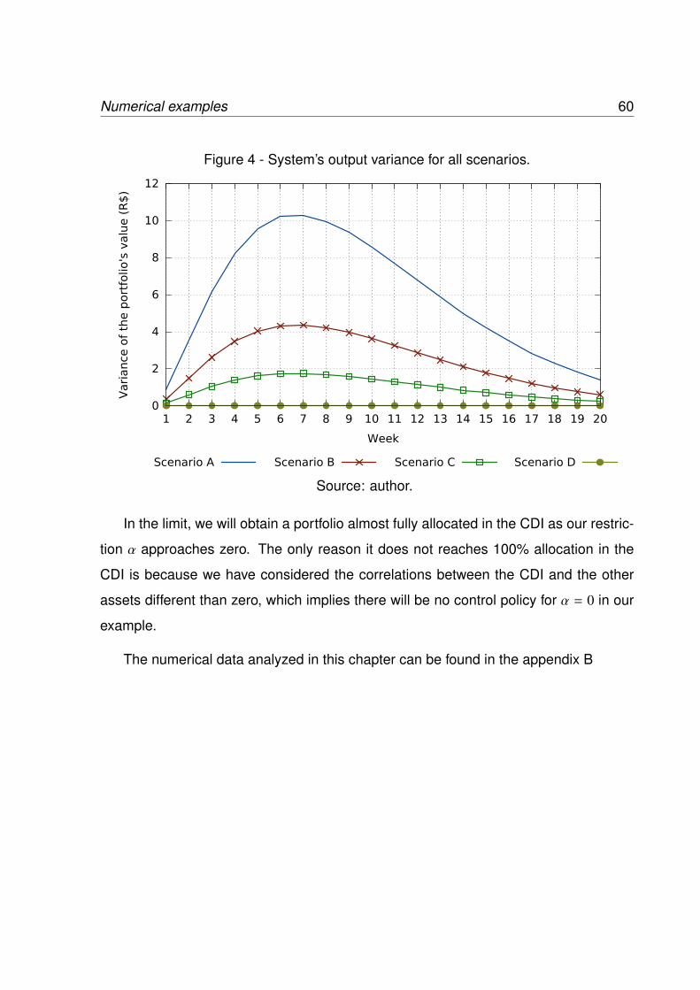
Numerical examples 60
Figure 4 - System’s output variance for all scenarios.
0
2
4
6
8
10
12
1 2 3 4 5 6 7 8 9 10 11 12 13 14 15 16 17 18 19 20
Vari
ance
of
the p
ort
folio
's v
alu
e (
R$
)
Week
Scenario A Scenario B Scenario C Scenario D
Source: author.
In the limit, we will obtain a portfolio almost fully allocated in the CDI as our restric-
tion α approaches zero. The only reason it does not reaches 100% allocation in the
CDI is because we have considered the correlations between the CDI and the other
assets different than zero, which implies there will be no control policy for α = 0 in our
example.
The numerical data analyzed in this chapter can be found in the appendix B

Numerical examples 61
Figure 5 - Control policy for scenario A.
-150
-130
-110
-90
-70
-50
-30
-10
10
30
50
70
90
1 2 3 4 5 6 7 8 9 10 11 12 13 14 15 16 17 18 19 20
Ass
et'
s allo
cati
on (
R$
)
Week
CDI EMBR3 ITUB4 PETR4 VALE5
Source: author.
Figure 6 - Control policy for scenario B.
-100-90-80-70-60-50-40-30-20-10
0 10 20 30 40 50 60 70
1 2 3 4 5 6 7 8 9 10 11 12 13 14 15 16 17 18 19 20
Ass
et'
s allo
cati
on (
R$
)
Week
CDI EMBR3 ITUB4 PETR4 VALE5
Source: Author.

Numerical examples 62
Figure 7 - Control policy for scenario C.
-60
-50
-40
-30
-20
-10
0
10
20
30
40
1 2 3 4 5 6 7 8 9 10 11 12 13 14 15 16 17 18 19 20
Ass
et'
s allo
cati
on (
R$
)
Week
CDI EMBR3 ITUB4 PETR4 VALE5
Source: Author.
Figure 8 - Control policy for scenario D.
-4
-3
-2
-1
0
1
2
3
1 2 3 4 5 6 7 8 9 10 11 12 13 14 15 16 17 18 19 20
Ass
et'
s allo
cati
on (
R$
)
Week
CDI EMBR3 ITUB4 PETR4 VALE5
Source: Author.

Numerical examples 63
6.2.2 Sensitivity analysis for β and ν
In the previous sections we described how to obtain the optimal allocation of assets
in a portfolio using our results and also provided a sensitivity analysis regarding the
restriction α. Now, our goal is to illustrate how the portfolio’s value, its variance and
optimal assets allocation changes with variations in one single element of both risk
parameters β and ν.
In this section, we simulate an arbitrary scenario where we say the investor wishes
to increase the portfolio’s value around step t = ta and decrease the portfolio’s volatility
around another step t = tb, which is achieved by adjusting the values of β(ta) and ν(tb),
respectively. The other way around or any other combination of possible scenarios
would lead to the same conclusions regarding the results’ sensitivity and, therefore,
were omitted in this analysis. Nonetheless, in the Appendix C, we provide further
sensitivity analysis for a diverse set of combinations of possible variations between the
elements of β and ν in order to illustrate the generalization of the conclusions laid out
here and summarized in the next section.
The portfolio’s assets and their characteristics are the same as described earlier in
Section 6.1. In order to facilitated the comparison among all scenarios, we will solve
the PC(ν, β, α) problem for the same arbitrary restriction, α = 100, in all scenarios and
run 10,000 simulations to compute the results for each of them.
We start with a base scenario, cc, where the vectors β and ν have all unitary el-
ements and then we apply a variation in a single element of each vector to assess
their effects on the portfolio’s results. In order to ease the graphical observation of
the variations in the results, we arbitrarily pick two specific time steps that are "suffi-
ciently" distant from each other and, in this case, we chose ta = 4 and tb = 9. Then we
set "big" enough new elements for β(4) and ν(9) in order to get visible changes in our
charts. After some try and error, we choose 3, 5, 7, 9, 11 as the set of possible new
coefficients’ values for illustration purposes and label the following scenarios using the
above rational, see Table 12.
We will focus the analysis based on four scenarios, cc, beta7, nu7, and

Numerical examples 64
Table 12 - Scenarios that combine specific changes in the coefficients of β and ν and abase scenario cc.
Input parameter
ResultingScenario Problem applied β(4) ν(9) α f (β, α)
cc PC(ν, β, α) 1 1 100 0.920beta7 PC(ν, β, α) 7 1 100 0.819nu7 PC(ν, β, α) 1 7 100 1.050
COMBINED-3 PC(ν, β, α) 3 3 100 0.939COMBINED-5 PC(ν, β, α) 5 5 100 0.937COMBINED-7 PC(ν, β, α) 7 7 100 0.925COMBINED-9 PC(ν, β, α) 9 9 100 0.907
COMBINED-11 PC(ν, β, α) 11 11 100 0.887
Note: β(t) = 1 and ν(t) = 1 for all the remaining t, t ∈ 1, · · · , 20 − 4, 9.
COMBINED − 7. This will allow us to see the specific effects around the scenario cc
by first changing β(4) to 7 in scenario beta7, by changing ν(9) to 7 in scenario nu7, and
then combining the effects of both changes in scenario COMBINED − 7. The remain-
ing scenarios will only be used to illustrated the sensitivity of the results of scenario
COMBINED − 7 for different levels of β(4) and ν(9).
Figures 9 and 10 show the portfolio’s value and its variance for the four scenarios
described above. As one can easily observe in the curve of beta7 versus cc, an increase
in β(4) leads to an increase in the portfolio’s value from t = 1 up to t = 4 followed by
a correspondent increase in the variance. After t = 4, β decreases back to 1 and the
portfolio’s value and its variance decreases.
In scenario nu7, we can see that an increase in ν(9) leads to a decrease in the
variance from t = 3 up to t = 9 followed by a correspondent decrease in the portfolio’s
value. Then, at t = 10, ν decreases back to 1 which leads to the opposite effect just
described.
Note that, given we imposed a restriction on the total variance for all scenarios,
α = 100, the higher variances obtained until t = 4 in scenario beta7 will be compensated
with lower variances in the later periods when compared with those from the base
scenario cc. The same reasoning applies for scenario nu7, where the restriction α = 100

Numerical examples 65
will force a compensation in the later periods leading them to show higher variances
when compared with those from the base scenario cc. The correspondent returns in the
later periods will follow their variances with the same trend of higher or lower values.
However, the accumulated returns will also influence the final results and it explains
why scenario beta7 showed a higher return than the one of scenario nu7 after t = 10.
As we can see in scenario COMBINED − 7, the combined effect of β(4) = 7 and
ν(9) = 7 leads to the same trends regarding the output and its variance as stated above.
However, now there are some compensation on the final results due to the opposite
effects of each variation.
Note that the parameters α = 100, β(4) = 7, and ν(9) = 7 will affect all the values
of the portfolio and their volatility over the whole time period, T = 20. However, the
strongest effect of β(4) and ν(9) are around t = 4 and t = 9, respectively, which means
that it is possible to be specific about the desired relevance of the portfolio’s value and
its volatility on each time step even though we can not be specific about the combined
result a priori.
It is also worth to mention that by setting a coefficient seven times higher than
any other coefficient does not mean achieving a portfolio’s value seven times higher
or a volatility seven times lower than otherwise. In our example, the portfolio’s value
increased from around 5 to 6 by choosing β(4) = 7, see curves cc and beta7 in Figure 9
at t = 4.

Numerical examples 66
Figure 9 - System’s output for scenario COMBINED− 7, beta7, nu7, and base scenario
cc.
0
2
4
6
8
10
12
14
16
18
20
1 2 3 4 5 6 7 8 9 10 11 12 13 14 15 16 17 18 19 20
Port
folio
's v
alu
e (
R$
)
Week
Scenario ccScenario COMBINED-7
Scenario beta7Scenario nu7
Source: Author.
Figure 10 - System’s output variance for scenario COMBINED−7, beta7, nu7, and base
scenario cc.
0
2
4
6
8
10
12
1 2 3 4 5 6 7 8 9 10 11 12 13 14 15 16 17 18 19 20
Vari
ance
of
the p
ort
folio
's v
alu
e (
R$
)
Week
Scenario ccScenario COMBINED-7
Scenario beta7Scenario nu7
Source: Author.

Numerical examples 67
Looking at the wealth allocation for scenarios COMBINED − 7 versus cc in Figure
11, we can see that setting a higher expected portfolio’s value through β(4) = 7 leads to
an increase in the wealth allocated in the risk assets and to a lower asset allocation in
the risk-free asset up to t = 4. In the same way, setting a lower volatility at t = 9 through
ν(9) = 7 forces the opposite effect on the wealth allocation.
Note that, after the point t = 9, the asset allocation tends to the one of scenario cc
because the values β(4) = 7 and ν(9) = 7 coincidentally counter-balanced each other
in this short period of time. However, this is not necessarily true if we choose other
values for α, β(t), and ν(t).
Figure 11 - Control policy for scenario COMBINED − 7 versus the base scenario cc.
-140
-110
-80
-50
-20
10
40
70
100
1 2 3 4 5 6 7 8 9 10 11 12 13 14 15 16 17 18 19 20
Ass
et'
s allo
cati
on (
R$
)
Week
CDI - COMBINED-7CDI - cc
EMBR3 - COMBINED-7EMBR3 - cc
ITUB4 - COMBINED-7
ITUB4 - ccPETR4 - COMBINED-7
PETR4 - ccVALE5 - COMBINED-7
VALE5 - cc
Source: Author.
The results for the remaining scenarios of Table 12 will lead to an identical con-
clusion to the one described above and, therefore, we will only show their results in
Figures 12 and 13 to illustrate the sensitivity of the output and the variance around
scenario cc for different values of β(4) and ν(9). Note that the variations in the portfo-
lio’s value and in its variance are not proportional to the changes in the coefficients,
illustrating our comments above.

Numerical examples 68
Figure 12 - System’s output for scenario COMBINED-5,6,7,8,9 and base scenario cc.
0
2
4
6
8
10
12
14
16
18
20
1 2 3 4 5 6 7 8 9 10 11 12 13 14 15 16 17 18 19 20
Port
folio
's v
alu
e (
R$
)
Week
Scenario ccScenario COMBINED-3Scenario COMBINED-5
Scenario COMBINED-7Scenario COMBINED-9
Scenario COMBINED-11
Source: Author.
Figure 13 - System’s output variance for scenario COMBINED-5, 6, 7, 8, 9 and base
scenario cc.
0
2
4
6
8
10
12
1 2 3 4 5 6 7 8 9 10 11 12 13 14 15 16 17 18 19 20
Vari
ance
of
the p
ort
folio
's v
alu
e (
R$
)
Week
Scenario ccScenario COMBINED-3Scenario COMBINED-5
Scenario COMBINED-7Scenario COMBINED-9
Scenario COMBINED-11
Source: Author.

Numerical examples 69
6.2.3 Sensitivity analysis summary and final comments
Following the above discussion and recalling the effects of α from the analysis
carried out in Section 6.2.1, we can summarize the effects that β, ν, and α will have
on the expected system’s output, its variance, and on the wealth allocation policy, see
Table 13.
Table 13 - Effects of changes in β, ν, and α on the expected portfolio’s value, its vari-ance, and on the wealth allocation policy.
Wealth allocation on
Risk parameter E[yu(t)] Var[yu(t)] risk assets risk-free asset
β(t) ↑ ↑ ↑ ↑ ↓
β(t) ↓ ↓ ↓ ↓ ↑
ν(t) ↑ ↓ ↓ ↓ ↑
ν(t) ↓ ↑ ↑ ↑ ↓
α ↑ ↑ ↑ ↑ ↓
α ↓ ↓ ↓ ↓ ↑
Note that these general effects are valid for variations within the elements of β and
ν as well as variations between the cross elements of those vectors.
Nonetheless, there is no standard or scientific procedure to determine the exactly
coefficients that someone should use as inputs for our risk parameters. In order to
understand and recognize the investor’s risk-aversion/risk-taking sentiment and the
trade-offs between β, ν, and α, we suggest a similar analysis to the one developed in
this chapter, where through modeling and testing different scenarios, someone would
be able to understand the potential gains and losses involved and what would be the
proper parameters inputs that represent his/her boundary conditions regarding returns
and variances over time.

70
7 CONCLUSION
In this work we have considered the stochastic multi-period optimal control problem
of discrete-time linear systems subject to Markov jumps and multiplicative noises. The
constrained problem analyzed, PC(ν, β, α), consisted in identifying the system’s control
law that maximizes the system’s output while restricting its total weighted variance by
the input parameter, α.
We provided an analytical solution of the PC(ν, β, α) problem using the optimal con-
trol policy of the unconstrained problem, PU(ν, ξ). This was achieved through the vari-
ance equation, which allowed us to establish an identity between ξ and α by defining ξ
as a multiple of β. Thus, the solution of PC(ν, β, α) extends previous results in the litera-
ture regarding our system by allowing it to be controlled with a maximum total weighted
variance, what was not possible before. Explicit conditions for the existence of an opti-
mal control strategy for the PC(ν, β, α) problem and an explicit way of calculating it were
presented in Chapter 5.
To illustrate the application of our results, we simulated a portfolio selection problem
with four risk assets and one risk-free security under the restriction of an arbitrary total
weighted variance limit. We also simulated the unconstrained problem, PU(ν, ξ), for
comparison purposes, and provided a sensitivity analysis for different risk parameters
α, ν, and β.
Regarding future developments we would consider as relevant the following topics:
1. Restriction on the variance in each time period. Providing an analytical solution
to the control law that takes into consideration a restriction on the maximum vari-
ance per period of time would be a significant improvement over our results and
it would also make the model more suitable for practical applications.
2. Restriction on the maximum and minimum limits allocated per asset. For a port-
folio manager, imposing such restrictions seems vital to the proper use of the
our system given that he/she usually has strict investment policies that limit the

Conclusion 71
portfolio exposure to specific assets, countries, currencies, leverage, etc.
3. Consideration of infinite time horizon. Pension funds is the classical example of
a type of investor which has an infinity time horizon and, therefore, a formulation
that takes this characteristic into consideration would be relevant to broaden the
kind of problem our model can handle and to spread its use with major investors.
4. Improvements on the methodology to estimate the operation modes and input
parameters. As we have cited, there are different approaches on how to estimate
the operation modes and input parameters, however, a blind application of them
may lead to undesired results. It would be of interest to develop and consolidate
the conditions and hypothesis that must guide anyone on the proper calculation
of our input parameters. For instance, parameters with non-stationary statistics
invalidate their use and, therefore, identifying these conditions seems to be very
relevant for any practical application of our model.

72
APPENDIX A -- DEMONSTRATION OF THEVECTOR FORMULATION INTHEOREM 2
In this section we want to prove that the Equation (4.25) can be rewritten in the
following useful vector form:
T∑t=1
ν(t)Var[yu(t)
]= λ′
(12
I − C′)Bλ − 2η′Bλ + c − η′a. (A.1)
where
c =
N∑i=1
tr( Pi(0)Qi(0) ), (A.2)
η = [a(1)ν(1) · · · a(T )ν(T )]′ = Γa, and (A.3)
C =
b(1, 1)ν(1) . . . b(1,T )ν(1)
... . . ....
b(T, 1)ν(T ) . . . b(T,T )ν(T )
= ΓB. (A.4)
Proof. The demonstration consists in expanding each of the three terms of Equation
(4.25) and rewriting each of them using the necessary definitions.
Expanding term 1 and applying the definitions of a and λ, we obtain that
T∑t=1
λ(t)a(t) = λ(1)a(1) + · · · + λ(T )a(T ) = a′λ. (A.5)

73
Expanding term 2 and applying the definitions of B and λ, we obtain that
T∑j=1
T∑i=1
λ( j)λ(i)b(i, j) =
λ(1)
[λ(1)b(1, 1) + . . . + λ(T )b(T, 1)
]+
+λ(2)[λ(1)b(1, 2) + . . . + λ(T )b(T, 2)
]+
. . . + λ(t)[λ(1)b(1,T ) + . . . + λ(T )b(T,T )
] =
= λ′Bλ. (A.6)
Expanding term 3, we have that
T∑t=1
λ(t) − ν(t)
[a(t) +
T∑s=1
λ(s)b(t, s)][
a(t) +
T∑s=1
λ(s)b(t, s)]
=
λ(1) − ν(1)
[a(1) + (λ(1)b(1, 1) + . . . + λ(T )b(1,T ))
]×
×[a(1) + (λ(1)b(1, 1) + . . . + λ(T )b(1,T ))
]+
λ(2) − ν(2)
[a(2) + (λ(1)b(2, 1) + . . . + λ(T )b(2,T ))
]×
×[a(2) + (λ(1)b(2, 1) + . . . + λ(T )b(2,T ))
]+ . . .+
+
λ(T ) − ν(T )
[a(T ) + (λ(1)b(T, 1) + . . . + λ(T )b(T,T ))
]×
×[a(T ) + (λ(1)b(T, 1) + . . . + λ(T )b(T,T ))
].
Applying the definitions of η and C into the above equation, we obtain that
T∑t=1
λ(t) − ν(t)
[a(t) +
T∑s=1
λ(s)b(t, s)][
a(t) +
T∑s=1
λ(s)b(t, s)]
=
=[λ − η − Cλ
]′ [a + Bλ
]=
[λ′ − η′ − λ′C′
] [a + Bλ
]= λ′a − η′a − λ′C′a + λ′Bλ − η′Bλ − λ′C′Bλ
= − η′a +(a′ − a′C − η′B
)λ + λ′
(B − C′B
)λ. (A.7)

74
Noticing that
a′C =
b(1, 1)a(1)ν(1) + · · · + b(T, 1)a(T )ν(T )
...
b(1,T )a(1)ν(1) + . . . + b(T,T )a(T )ν(T )
= η′B, (A.8)
Equation (A.7) can be rewritten as
T∑t=1
λ(t) − ν(t)
[a(t) +
T∑s=1
λ(s)b(t, s)][
a(t) +
T∑s=1
λ(s)b(t, s)]
= − η′a +(a′ − a′C − η′B
)λ + λ′
(B − C′B
)λ
= − η′a + a′λ − 2η′Bλ + λ′(B − C′B
)λ. (A.9)
Substituting (A.5), (A.6) and (A.9) into (4.25), we have that
T∑t=1
ν(t)Var[yu(t)
]= c − a′λ −
12λ′Bλ − η′a + a′λ − 2η′Bλ + λ′
(B − C′B
)λ
⇔
T∑t=1
ν(t)Var[yu(t)
]= λ′
(12
I − C′)Bλ − 2η′Bλ + c − η′a, (A.10)
completing the demonstration.

75
APPENDIX B -- NUMERICAL DATA OFSIMULATIONS OF SECTION6.2.1
Table 14 - System’s output for all scenarios.Time Scenario 1 Scenario 2 Scenario 3 Scenario 4
1 1.3 1.2 1.1 1.02 2.4 1.9 1.6 1.03 3.7 2.8 2.1 1.14 5.2 3.7 2.7 1.25 6.7 4.7 3.4 1.26 8.2 5.7 4.0 1.37 9.7 6.7 4.6 1.38 11.1 7.6 5.2 1.49 12.4 8.4 5.7 1.4
10 13.6 9.2 6.2 1.411 14.7 9.9 6.7 1.512 15.7 10.6 7.1 1.513 16.7 11.2 7.5 1.514 17.5 11.7 7.8 1.515 18.3 12.2 8.1 1.616 18.9 12.7 8.4 1.617 19.5 13.1 8.6 1.618 20.0 13.4 8.9 1.619 20.5 13.7 9.0 1.620 20.9 13.9 9.2 1.6

76
Table 15 - System’s output variance for all scenarios.Time Scenario 1 Scenario 2 Scenario 3 Scenario 4
1 0.86 0.37 0.15 0.00072 3.54 1.50 0.60 0.0033 6.19 2.62 1.05 0.0054 8.25 3.49 1.40 0.0075 9.58 4.05 1.62 0.0086 10.21 4.32 1.73 0.0097 10.30 4.36 1.74 0.0098 9.97 4.22 1.69 0.0089 9.37 3.96 1.58 0.008
10 8.58 3.63 1.45 0.00711 7.70 3.25 1.30 0.00712 6.78 2.87 1.15 0.00613 5.87 2.48 0.99 0.00514 5.01 2.12 0.85 0.00415 4.20 1.78 0.71 0.00416 3.48 1.47 0.59 0.00317 2.84 1.20 0.48 0.00218 2.28 0.97 0.39 0.00219 1.81 0.77 0.31 0.00220 1.42 0.60 0.24 0.001
Table 16 - Control policy for scenario A.Time CDI EMBR3 ITUB4 PETR4 VALE5
0 -137.9 -24.9 87.1 9.8 66.91 -138.7 -21.8 88.5 15.5 57.82 -136.0 -20.0 87.3 17.4 53.63 -126.9 -18.2 82.3 17.4 49.14 -116.2 -16.5 76.4 17.0 44.55 -109.6 -15.5 72.9 16.3 42.66 -100.9 -14.3 68.3 15.6 39.67 -94.8 -13.3 65.1 14.8 37.88 -87.0 -12.0 60.9 14.2 35.09 -73.2 -11.0 53.5 12.5 30.610 -65.9 -10.0 49.4 11.5 28.511 -51.4 -9.2 41.5 9.6 24.212 -43.2 -8.4 37.0 8.3 22.013 -37.8 -7.2 34.1 7.9 19.714 -29.9 -6.4 29.7 6.9 17.215 -23.2 -5.4 25.9 6.1 14.816 -16.6 -4.6 22.2 5.2 12.817 -12.7 -3.9 20.0 4.7 11.418 -7.0 -3.3 16.8 3.9 9.719 -1.6 -2.7 13.7 3.3 7.7

77
Table 17 - Control policy for scenario B.Time CDI EMBR3 ITUB4 PETR4 VALE5
0 -89.3 -16.2 56.6 6.4 43.51 -89.3 -14.0 57.2 10.2 37.12 -85.8 -12.9 55.4 11.0 34.23 -80.5 -11.8 52.6 11.1 31.54 -76.7 -11.1 50.5 11.0 30.05 -74.3 -10.3 49.4 11.0 28.96 -63.1 -9.4 43.2 9.7 25.47 -57.4 -8.6 40.2 9.2 23.38 -50.3 -7.9 36.3 8.4 21.19 -45.8 -7.2 33.9 7.9 19.5
10 -38.0 -6.6 29.6 6.7 17.411 -35.3 -5.8 28.2 6.6 16.312 -29.3 -5.3 25.0 5.8 14.413 -24.1 -4.6 22.0 5.2 12.714 -19.0 -4.2 19.2 4.3 11.415 -14.9 -3.6 17.0 3.9 9.916 -10.5 -3.1 14.4 3.3 8.517 -7.1 -2.6 12.6 3.0 7.218 -4.4 -2.1 11.0 2.6 6.219 -0.3 -1.7 8.7 2.1 4.9
Table 18 - Control policy for scenario C.Time CDI EMBR3 ITUB4 PETR4 VALE5
0 -56.1 -10.2 35.8 4.0 27.51 -57.5 -9.0 36.9 6.5 24.12 -54.8 -8.3 35.5 7.0 22.03 -51.8 -7.5 34.0 7.2 20.34 -48.8 -7.0 32.4 7.1 19.15 -44.2 -6.3 29.9 6.8 17.26 -40.5 -5.8 27.9 6.4 16.17 -36.3 -5.3 25.6 5.9 14.68 -32.6 -4.9 23.6 5.5 13.69 -28.4 -4.6 21.4 4.9 12.4
10 -26.0 -4.2 20.1 4.6 11.611 -21.7 -3.7 17.8 4.1 10.212 -18.1 -3.4 15.8 3.6 9.113 -15.7 -2.9 14.4 3.4 8.214 -12.1 -2.6 12.4 2.9 7.115 -9.2 -2.2 10.8 2.5 6.316 -5.5 -1.9 8.7 2.1 5.017 -3.8 -1.6 7.7 1.8 4.518 -1.8 -1.3 6.6 1.6 3.819 0.2 -1.1 5.5 1.3 3.1

78
Table 19 - Control policy for scenario D.Time CDI EMBR3 ITUB4 PETR4 VALE5
0 -3.0 -0.7 2.5 0.3 1.91 -3.1 -0.6 2.6 0.5 1.72 -2.9 -0.6 2.5 0.5 1.53 -2.7 -0.5 2.4 0.5 1.44 -2.5 -0.5 2.3 0.5 1.35 -2.2 -0.5 2.1 0.5 1.36 -2.0 -0.4 2.0 0.5 1.27 -1.8 -0.4 1.9 0.4 1.18 -1.5 -0.3 1.7 0.4 1.09 -1.1 -0.3 1.5 0.5 0.910 -0.9 -0.3 1.4 0.3 0.811 -0.6 -0.3 1.2 0.3 0.712 -0.3 -0.2 1.1 0.3 0.613 -0.1 -0.2 1.0 0.2 0.614 0.2 -0.2 0.9 0.2 0.515 0.3 -0.2 0.8 0.2 0.416 0.5 -0.1 0.7 0.2 0.417 0.7 -0.1 0.6 0.1 0.318 0.9 -0.9 0.5 0.1 0.319 1.0 -0.1 0.4 0.1 0.2

79
APPENDIX C -- FURTHER SENSITIVITYANALYSIS OF β AND ν
In this appendix we extend the sensitivity analysis of the risk parameters β and ν
we provided in Chapter 6. Now, we define other scenarios depending on the different
relative values of β and ν illustrating the results generalized in Table 13.
As previously stated, this type of sensitivity should help the investor to understand
how the portfolio’s variables may behave given his/her risk preferences and to assist
him/her on the task of choosing the coefficients of β and ν.
The portfolio’s assets and their characteristics are the same as described earlier in
Section 6.1. In order to facilitated the comparison among all scenarios, we will solve
the PC(ν, β, α) problem for the same arbitrary restriction, α, in all scenarios and run
10,000 simulations to compute the results for each of them. As described in Chapter
5, solving this problem implies that, given the risk parameters β and ν and a maximum
total variance, α, one could obtain the optimal control, u(k), following the steps given in
Section 4.7 and computing ξ using Equation (5.10).
We also arbitrarily define our risk parameters in order to keep the different results in
a scale that would ease the observation of trends in the charts below. Notwithstanding,
the analysis made here will be valid for different boundaries and restrictions that the
investor may choose regarding the risk parameters as long as they do not violate the
limits of our hypothesis laid out in the theorems and propositions of Chapters 4 and 5.
Thus, we set α = 100.0 for all scenarios as before and define different scenarios
by considering that the elements of β and ν may assume three possible behaviors over
time: i) stay at a constant level equal to 1 or to a multiple of 1, ii) go up linearly from 1

80
to 10, or iii) go down linearly from 10 to 1.
We will split the analysis into the following sections. Section C.1 shows the port-
folio’s behavior when we change the vectors β and ν by multiples and, in Section C.2,
we simulate the portfolio’s behavior for different combinations of β and ν assuming they
can either have a constant shape, an upward trend shape, or a downward trend shape
over time.
C.1 Simulations for different constant levels of β and ν
In this section, our goal is to analyze what happens with the portfolio’s behavior
when we change a given vector β or ν by multiples of themselves. We will consider four
scenarios where all elements of β and ν have constant and identical elements equal to
1, 2, 4, or 8. Then we solve the PC(ν, β, α) problem to obtain the optimal control law in
each scenario.
The scenarios labels and inputs are shown in Table 20 while in Figure 14 we show
an illustration of the values that the elements of β and ν take over time in each scenario.
Table 20 - Scenarios when β and ν are constants and resulting f (β, α) of problemPC(ν, β, α).
Risk parameters’behavior fort = 1, 2, . . . ,T
ResultingScenario Problem applied β(t) ν(t) α f (β, α)
cc PC(ν, β, α) 1 1 100 0.920cc2 PC(ν, β, α) 2 2 100 0.650cc4 PC(ν, β, α) 4 4 100 0.460cc8 PC(ν, β, α) 8 8 100 0.325
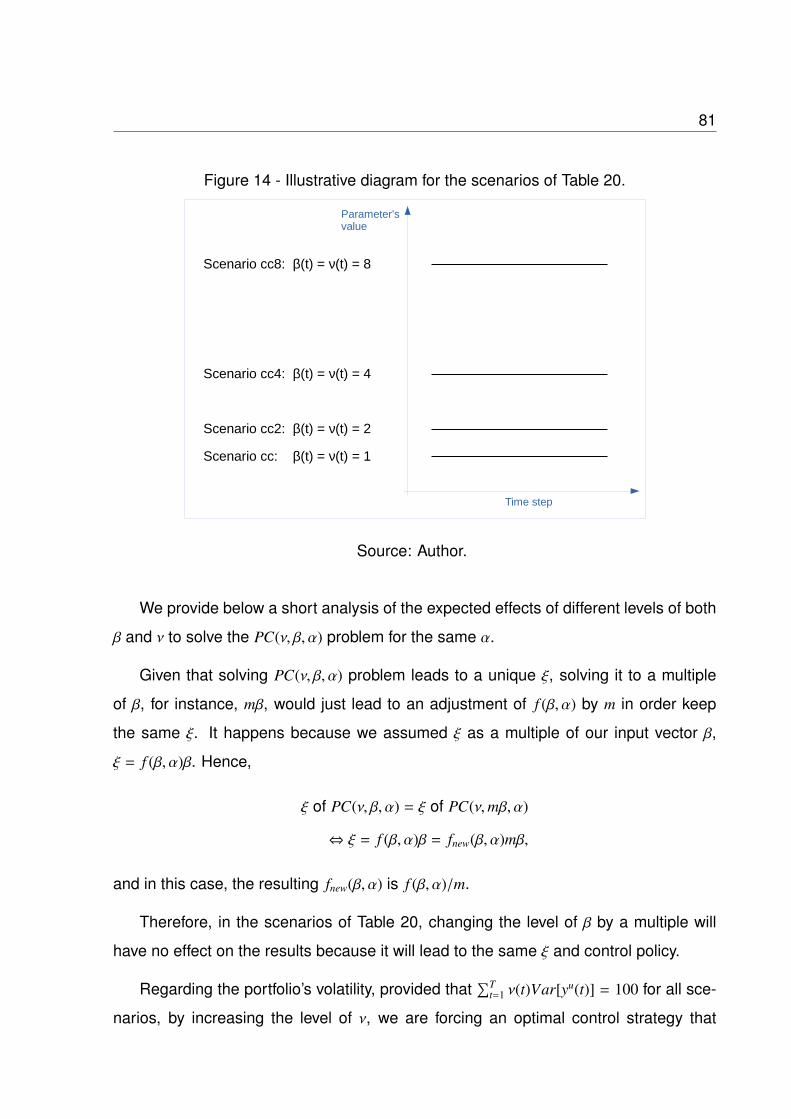
81
Figure 14 - Illustrative diagram for the scenarios of Table 20.
Scenario cc8: β(t) = ν(t) = 8
Scenario cc: β(t) = ν(t) = 1
Scenario cc2: β(t) = ν(t) = 2
Scenario cc4: β(t) = ν(t) = 4
Time step
Parameter's value
Source: Author.
We provide below a short analysis of the expected effects of different levels of both
β and ν to solve the PC(ν, β, α) problem for the same α.
Given that solving PC(ν, β, α) problem leads to a unique ξ, solving it to a multiple
of β, for instance, mβ, would just lead to an adjustment of f (β, α) by m in order keep
the same ξ. It happens because we assumed ξ as a multiple of our input vector β,
ξ = f (β, α)β. Hence,
ξ of PC(ν, β, α) = ξ of PC(ν,mβ, α)
⇔ ξ = f (β, α)β = fnew(β, α)mβ,
and in this case, the resulting fnew(β, α) is f (β, α)/m.
Therefore, in the scenarios of Table 20, changing the level of β by a multiple will
have no effect on the results because it will lead to the same ξ and control policy.
Regarding the portfolio’s volatility, provided that∑T
t=1 ν(t)Var[yu(t)] = 100 for all sce-
narios, by increasing the level of ν, we are forcing an optimal control strategy that

82
achieves a lower total variance. Note that it is the total weighted variance that has
been kept constant, not the total variance alone. Thus, setting α = 100 and ν(t) = 1,∀t,
leads to the same results of setting α = 50 and ν(t) = 2, or α = 25 and ν(t) = 4, etc.
Therefore, given that any multiple of β does not change the results and that higher
multiples of ν imply in solving an equivalent problem where α decreases, the result-
ing portfolio’s behavior of the scenarios in Table 20 will follow the same behavior as
described in Section 6.2.
Thereby, as one can see in Figures 15 and 16, the portfolio’s value gets lower as ν
increases. Once more, a lower total variance is achieved indirectly in these particular
scenarios because∑T
t=1 ν(t)Var[yu(t)] = 100 is kept constant while ν increases.
Figure 15 - System’s output when β and ν are constants.
0
2
4
6
8
10
12
14
16
18
20
1 2 3 4 5 6 7 8 9 10 11 12 13 14 15 16 17 18 19 20
Port
folio
's v
alu
e (
R$
)
Week
Scenario ccScenario cc2
Scenario cc4Scenario cc8
Source: Author.

83
Figure 16 - System’s output variance when β and ν are constants.
0
1
2
3
4
5
6
7
8
9
1 2 3 4 5 6 7 8 9 10 11 12 13 14 15 16 17 18 19 20
Vari
ance
of
the p
ort
folio
's v
alu
e (
R$
)
Week
Scenario ccScenario cc2
Scenario cc4Scenario cc8
Source: Author.
In the same way as in Section 6.2, the imposition of a lower total variance will lead
to an increase in the wealth allocation on the risk-free asset, CDI, while decreasing
proportionally the wealth allocation on the risk assets as we can see in Figures 17, 18,
19, and 20.

84
Figure 17 - Control policy for scenario cc.
-150
-130
-110
-90
-70
-50
-30
-10
10
30
50
70
90
1 2 3 4 5 6 7 8 9 10 11 12 13 14 15 16 17 18 19 20
Ass
et'
s allo
cati
on (
R$
)
Week
CDI EMBR3 ITUB4 PETR4 VALE5
Source: Author.
Figure 18 - Control policy for scenario cc2.
-150
-130
-110
-90
-70
-50
-30
-10
10
30
50
70
90
1 2 3 4 5 6 7 8 9 10 11 12 13 14 15 16 17 18 19 20
Ass
et'
s allo
cati
on (
R$
)
Week
CDI EMBR3 ITUB4 PETR4 VALE5
Source: Author.

85
Figure 19 - Control policy for scenario cc4.
-150
-130
-110
-90
-70
-50
-30
-10
10
30
50
70
90
1 2 3 4 5 6 7 8 9 10 11 12 13 14 15 16 17 18 19 20
Ass
et'
s allo
cati
on (
R$
)
Week
CDI EMBR3 ITUB4 PETR4 VALE5
Source: Author.
Figure 20 - Control policy for scenario cc8.
-150
-130
-110
-90
-70
-50
-30
-10
10
30
50
70
90
1 2 3 4 5 6 7 8 9 10 11 12 13 14 15 16 17 18 19 20
Ass
et'
s allo
cati
on (
R$
)
Week
CDI EMBR3 ITUB4 PETR4 VALE5
Source: Author.

86
C.2 Simulations for different combinations of β and ν
In this section we will expand the sensitivity analysis of the risk parameters β and
ν for different combinations of them over time. Our goal is to understand the different
trade-offs between the portfolio’s value, variance, and asset allocation when we impose
different weights to the elements of β and ν.
Now, we will consider variations within the elements of β and ν, assuming they
either do not change or change linearly over time in an upward or downward trend. In
the timeline, the elements of β and ν will form a curve, or shape, that we will refer to as
"behavior" of β and ν.
The equations that describe these behaviors, see Table 21, were chosen arbitrar-
ily in order to illustrate the potential relative trends between β and ν, and within their
elements. Thus, we will verify the portfolio results when the elements of β increases
while ν is kept constant, or when the elements of β decreases while the elements of ν
increases, etc.
Once again, the boundaries of each behavior were chosen in order to keep the
different results in a scale that would ease the observation of the trends.
Table 21 - Behaviors definitions for β and ν.
Input parameter’s equations fort = 1, 2, . . . , 20
Behavior β(t) ν(t)
constant 1 1up (9/19)*(t-1) + 1 (9/19)*t + 1
down (9/19)*(20-t) + 1 (9/19)*(20-t) + 1
We then grouped the nine potential combinations of the three behaviors (constant,
up, and down) in scenarios as described in Table 22 and illustrated in Figure 21.

87
Table 22 - Scenarios that combine different β and ν behaviors and resulting f (β, α) ofproblem PC(ν, β, α).
Risk parameter’sbehavior
ResultingScenario Problem applied β ν α f (β, α)
uc PC(ν, β, α) up constant 100 0.132cc PC(ν, β, α) constant constant 100 0.920dc PC(ν, β, α) down constant 100 0.220ud PC(ν, β, α) up down 100 0.285cd PC(ν, β, α) constant down 100 2.128dd PC(ν, β, α) down down 100 0.559uu PC(ν, β, α) up up 100 0.283cu PC(ν, β, α) constant up 100 1.878du PC(ν, β, α) down up 100 0.418
Figure 21 - Illustrative diagram for the scenarios of Table 22.
dc uc uu du
cu cd dd ud
cc
Curve's shape for βCurve's shape for ν
Legend:
Source: Author.
Finally, Figures 22 and 23 illustrate the portfolio’s value and its volatility for all nine
scenarios. Their analysis will be split in the next 5 sections in order to make it easy to
see the effects that each change is causing in the overall results.

88
Figure 22 - System’s output for the scenarios of Table 22.
0
2
4
6
8
10
12
14
16
18
20
22
1 2 3 4 5 6 7 8 9 10 11 12 13 14 15 16 17 18 19 20
Port
folio
's v
alu
e (
R$
)
Week
Scenario ucScenario ccScenario dc
Scenario udScenario cdScenario dd
Scenario uuScenario cuScenario du
Source: Author.
Figure 23 - System’s output variance for the scenarios of Table 22.
0
2
4
6
8
10
12
1 2 3 4 5 6 7 8 9 10 11 12 13 14 15 16 17 18 19 20
Vari
ance
of
the p
ort
folio
's v
alu
e (
R$
)
Week
Scenario ucScenario ccScenario dc
Scenario udScenario cdScenario dd
Scenario uuScenario cuScenario du
Source: Author.

89
C.2.1 Sensitivity analysis when α is not applied
The scenarios above, Table 22, were established considering we are solving
PC(ν, β, α) to obtain the optimal wealth allocation.
However, in order to compare the effects of imposing α, we also obtained the simu-
lations of each of the nine scenarios from Table 22 considering no restriction α. This is
achieved by solving PU(ν, ξ), where ξ will take the same behavior as β in each scenario.
In Table 23, we show the scenarios as before with the symbol "*" to indicate that it is
being applied PU(ν, ξ) instead of PC(ν, β, α). There, we can also see the resulting total
weighted variance for each scenario.
Table 23 - Resulting total weighted variance for the scenarios of Table 22 when thereis no restriction α.
Risk parameter’s Resulting totalbehavior weighted variance
Scenario Problem applied ξ ν∑T
t=1 ν(t)Var[yu(t)]
uc* PU(ν, ξ) up constant 5784.5cc* PU(ν, ξ) constant constant 118.2dc* PU(ν, ξ) down constant 2070.2ud* PU(ν, ξ) up down 1227.2cd* PU(ν, ξ) constant down 22.1dd* PU(ν, ξ) down down 319.6uu* PU(ν, ξ) up up 1251.3cu* PU(ν, ξ) constant up 28.4du* PU(ν, ξ) down up 574.4
The resulting portfolio’s value and its variance using PU(ν, ξ) were depicted in Fig-
ures 24 and 26, respectively, and their zooms in Figures 25, 27, and 28.

90
Figure 24 - System’s output for the scenarios of Table 23.
0
20
40
60
80
100
120
140
160
1 2 3 4 5 6 7 8 9 10 11 12 13 14 15 16 17 18 19 20
Port
folio
's v
alu
e (
R$
)
Week
Scenario uc*Scenario cc*Scenario dc*
Scenario ud*Scenario cd*Scenario dd*
Scenario uu*Scenario cu*Scenario du*
Source: Author.
Figure 25 - Zoom of Figure 24.
0
5
10
15
20
25
30
35
40
1 2 3 4 5 6 7 8 9 10 11 12 13 14 15 16 17 18 19 20
Port
folio
's v
alu
e (
R$
)
Week
Scenario uc*Scenario cc*Scenario dc*
Scenario ud*Scenario cd*Scenario dd*
Scenario uu*Scenario cu*Scenario du*
Source: Author.

91
Figure 26 - System’s output variance for the scenarios of Table 23.
0
50
100
150
200
250
300
350
400
450
500
1 2 3 4 5 6 7 8 9 10 11 12 13 14 15 16 17 18 19 20
Vari
ance
of
the p
ort
folio
's v
alu
e (
R$
)
Week
Scenario uc*Scenario cc*Scenario dc*
Scenario ud*Scenario cd*Scenario dd*
Scenario uu*Scenario cu*Scenario du*
Source: Author.
Figure 27 - Zoom of Figure 26.
0
5
10
15
20
25
30
35
1 2 3 4 5 6 7 8 9 10 11 12 13 14 15 16 17 18 19 20
Vari
ance
of
the p
ort
folio
's v
alu
e (
R$
)
Week
Scenario uc*Scenario cc*Scenario dc*
Scenario ud*Scenario cd*Scenario dd*
Scenario uu*Scenario cu*Scenario du*
Source: Author.

92
Figure 28 - Zoom of Figure 27.
0
1
2
3
4
5
1 2 3 4 5 6 7 8 9 10 11 12 13 14 15 16 17 18 19 20
Vari
ance
of
the p
ort
folio
's v
alu
e (
R$
)
Week
Scenario uc*Scenario cc*Scenario dc*
Scenario ud*Scenario cd*Scenario dd*
Scenario uu*Scenario cu*Scenario du*
Source: Author.
The analysis laid out in the following paragraphs compares the returns and vari-
ances with the restriction α = 100, Figures 22 and 23, with their respective scenarios
when there is no restriction, Figures 24 and 26. When necessary, one should consider
Figures 24 and 26’s zooms in Figures 25, 27, and 28 for a better view.
In this way, we can see that when we solve PC(ν, β, α) with a restriction α that is
higher than the total weighted variance that we would have had without this restriction,
then we get higher variances and returns over the whole period of time, see scenarios
cd∗ and cu∗ in Table 23, where∑T
t=1 ν(t)Var[yu(t)] < 100.
On the other hand, in the remaining scenarios of Table 23,∑T
t=1 ν(t)Var[yu(t)] > 100
and, therefore, we obtain lower returns and variances over the whole period of time
when we impose them α = 100, see Figures 22 and 23 versus Figures 24 and 26.
The effects on the wealth allocation for the scenarios without the restriction α were
omitted because they will follow the same pattern as extensively illustrated in the follow-
ing analysis for the PC(ν, β, α) problem, which is a higher allocation on the risk assets

93
versus the risk-free asset, whenever a higher return or variance are demanded and
conversely, a lower allocation on the risk assets versus the risk-free asset, whenever a
lower return or variance are demanded.
Given we only needed to solve PU(ν, ξ) here to show the sensitivity of our results
when there is no α, we will proceed with the analysis in the remaining sections by
focusing only in the scenarios of Table 22, where only PC(ν, β, α) is applied.
C.2.2 Analysis for scenarios uc and dc
We first evaluate the effects of β when ν is kept constant, scenarios uc and dc,
around the base scenario where both are constants, scenario cc.
Analyzing Figures 22 and 23, we can see that choosing β that increases over time
leads to a higher return and variance on the later steps and to a lower return and vari-
ance in the earlier steps in relation to the base scenario, cc. Therefore, the upward
β has the effect of rotating both the expected return and variance curves counter-
clockwise around scenario cc. This is achieved by decreasing the wealth allocation
in the risk assets in the earlier periods and increasing the wealth allocation in the same
assets in the later periods when compared with the base scenario cc, see Figure 29
with the asset’s allocation for scenarios uc and cc.
Conversely, choosing a β that decreases over time leads to a lower return and
variance on the later steps and to a higher return and variance in the earlier steps in
relation to the base scenario, cc. Therefore, the downward β has the effect of rotating
both the expected return and variance curves clockwise around scenario cc. This be-
havior is achieved by increasing the wealth allocation in the risk assets in the earlier
periods and decreasing the wealth allocation in the same assets in the later periods
when compared with the base scenario cc, see Figure 30 for scenarios dc and cc.

94
Figure 29 - Control policy for scenario uc versus scenario cc.
-130
-110
-90
-70
-50
-30
-10
10
30
50
70
90
1 2 3 4 5 6 7 8 9 10 11 12 13 14 15 16 17 18 19 20
Ass
et'
s allo
cati
on (
R$
)
Week
CDICDI - ccEMBR3
EMBR3 - ccITUB4
ITUB4 - cc
PETR4PETR4 - cc
VALE5
VALE5 - cc
Source: Author.
Figure 30 - Control policy for scenario dc versus scenario cc.
-170-150-130-110
-90-70-50-30-10 10 30 50 70 90
110
1 2 3 4 5 6 7 8 9 10 11 12 13 14 15 16 17 18 19 20
Ass
et'
s allo
cati
on (
R$
)
Week
CDICDI - ccEMBR3
EMBR3 - ccITUB4
ITUB4 - cc
PETR4PETR4 - cc
VALE5
VALE5 - cc
Source: Author.

95
The fact that a higher β in the early steps of scenario uc did not lead to higher
returns relative to the cc scenario is due to the restriction α that will impose a lower
return over all steps. Without the restriction α, the returns would had been higher for all
steps as well as their variances, see Figures 24 and 26 for simulations of the scenarios
when α is not applied. Therefore, it is the restriction α that creates the impression of a
counter-clockwise shift around scenario cc when β increases over time.
The same rational is true for scenario dc, but now the relative smallest coefficients
appear in the second half of our timeline and, therefore, the expected returns and
variances are more penalized from t = 10 to t = 20, creating the impression of a
clockwise shift around scenario cc.
C.2.3 Analysis for scenarios cd and cu
The assessment of the scenarios where β is kept constant while ν varies, cd and
cu, will also be analyzed around the base scenario where both are constants, cc.
In Figure 23, we can see that choosing a ν that increases over time leads to a lower
variance in the later steps in comparison with the earlier steps. Conversely, a ν that
decreases over time leads to a higher variance in the later steps when compared with
the variance in the earlier steps. It means that the higher the risk aversion ν(t), the
lower will be the variance at t.
Provided that we are solving the PC(ν, β, α) problem, the overall variance were re-
duced to comply with the imposed restriction, α = 100, when compared with the base
scenario cc. Therefore, setting higher values for ν in scenarios cd and cu than in cc will
lead to lower variances in those scenarios than in scenario cc, see in Figure 23.
Regarding the portfolio’s return for scenarios cd, cu and cc, we can observe in
Figure 22 that the imposition of a lower variance led to lower returns and conversely,
the allowance of higher variance led to higher returns.
This behavior is achieved by decreasing the wealth allocation on the risk assets
over the periods with a higher ν, lower variances allowed, and by increasing the wealth

96
allocation on the risk assets over the periods with a lower ν, higher variances allowed,
see Figures 31 and 32 for a comparison of the assets’ allocation in scenario cd and cu
versus cc.
Figure 31 - Control policy for scenario cd versus scenario cc.
-130
-110
-90
-70
-50
-30
-10
10
30
50
70
90
1 2 3 4 5 6 7 8 9 10 11 12 13 14 15 16 17 18 19 20
Ass
et'
s allo
cati
on (
R$
)
Week
CDICDI - ccEMBR3
EMBR3 - ccITUB4
ITUB4 - cc
PETR4PETR4 - cc
VALE5
VALE5 - cc
Source: Author.
Figure 32 - Control policy for scenario cu versus scenario cc.
-130
-110
-90
-70
-50
-30
-10
10
30
50
70
90
1 2 3 4 5 6 7 8 9 10 11 12 13 14 15 16 17 18 19 20
Ass
et'
s allo
cati
on (
R$
)
Week
CDICDI - ccEMBR3
EMBR3 - ccITUB4
ITUB4 - cc
PETR4PETR4 - cc
VALE5
VALE5 - cc
Source: Author.

97
C.2.4 Analysis for scenarios ud and dd
In order to analyze the effects of changing β when ν has a downward trend, we will
compare the results around the scenario where β is constant and ν has a downward
trend, cd.
Therefore, observing the curves ud and dd around the curve cd in Figures 22 and
23, we can conclude that the increase of β(t) leads to a higher return and variance at t
and, a decrease of β(t) leads to a lower return and variance at t.
As explained above, the restriction α leads to the impression of shifting the port-
folio’s value in a counter-clockwise direction around the scenario cd when β has an
upward trend, as in scenario ud, and shifting it in a clockwise direction when β has an
downward trend, as in scenario dd.
Once more, the downward trend of ν led to lower variances and returns over the
earlier steps than in the later steps when compared with the curves uu, cu, and du for
the reasons already exposed before.
When we compare all curves where ν has a downward trend (ud, cd, dd) with all
curves where ν is constant (uc, cc, dc), see Figure 23, we can observe that the average
higher values of ν in the first block leads to lower variances over time. Once more, this
effect is explained by the imposition of the restriction α that "forces" a lower variance
even when we set a lower ν. Note how a lower ν leads to higher variances when α is
not applied in Figure 27 for the same scenarios mentioned here.
The control policy, shown in Figures 33 and 34, confirm the same effect as ob-
served in Section C.2.2, which is that higher elements of β lead to a higher exposure to
risk assets and conversely, lower elements of β lead to a lower exposure to risk assets

98
Figure 33 - Control policy for scenario ud versus scenario cd.
-50
-40
-30
-20
-10
0
10
20
30
40
1 2 3 4 5 6 7 8 9 10 11 12 13 14 15 16 17 18 19 20
Ass
et'
s allo
cati
on (
R$
)
Week
CDICDI - cdEMBR3
EMBR3 - cdITUB4
ITUB4 - cd
PETR4PETR4 - cd
VALE5
VALE5 - cd
Source: Author.
Figure 34 - Control policy for scenario dd versus scenario cd.
-50
-40
-30
-20
-10
0
10
20
30
40
1 2 3 4 5 6 7 8 9 10 11 12 13 14 15 16 17 18 19 20
Ass
et'
s allo
cati
on (
R$
)
Week
CDICDI - cdEMBR3
EMBR3 - cdITUB4
ITUB4 - cd
PETR4PETR4 - cd
VALE5
VALE5 - cd
Source: Author.

99
C.2.5 Analysis for scenarios uu and du
In our last scenarios, uu and du, we consider the variation of β when ν keeps an
upward trend and we will compare these scenarios with the base scenario where β is
constant, cu.
As in the previous Section C.2.4, by observing Figures 22 and 23, we can conclude
that the increase of β over time leads to a higher return and variance, and a decrease
of β leads to a lower return and variance. However, now the increase in the returns is
not so strong in the later steps because it is has been counterbalanced by a higher ν
in those periods. Recall that higher elements of ν imposes a lower return and variance
as we can verify when we compare the curves for ud, cd, and dd versus uu, cu, and du
in Figures 22 and 23.
The control policy, shown in Figures 35 and 36, once more confirms the same effect
already observed, which is that higher elements of β lead to a higher exposure to risk
assets and conversely, lower elements of β lead to a lower exposure to risk assets.
Note that, even though the comparison of the allocation curves is hard after the
step 12, it is still possible to observe where the curves of uu and du cross the curves
of cu. It is also clear the shift caused by a higher β in scenario uu, and a lower β in
scenario du in the early steps.

100
Figure 35 - Control policy for scenario uu versus scenario cu.
-140
-110
-80
-50
-20
10
40
70
100
1 2 3 4 5 6 7 8 9 10 11 12 13 14 15 16 17 18 19 20
Ass
et'
s allo
cati
on (
R$
)
Week
CDICDI - cuEMBR3
EMBR3 - cuITUB4
ITUB4 - cu
PETR4PETR4 - cu
VALE5
VALE5 - cu
Source: Author.
Figure 36 - Control policy for scenario du versus scenario cu.
-170
-140
-110
-80
-50
-20
10
40
70
100
1 2 3 4 5 6 7 8 9 10 11 12 13 14 15 16 17 18 19 20
Ass
et'
s allo
cati
on (
R$
)
Week
CDICDI - cuEMBR3
EMBR3 - cuITUB4
ITUB4 - cu
PETR4PETR4 - cu
VALE5
VALE5 - cu
Source: Author.

101
REFERENCES
BARBIERI, F.; COSTA, O. L. V. Linear systems with markov jumps andmultiplicative noises - constrained total variance problem. In: . Vitória, EspíritoSanto - Brasil: Congresso Brasileiro de Automação, 2016.
CAKMAK, U.; OZECKICI, S. Portfolio optimization in stochastic markets.Mathematical Methods of Operations Research, v. 63, p. 151–168, 2006.
CANAKOGLU, E.; OZECKICI, S. Portfolio selection in stochastic markets withhara utility functions. European Journal of Operational Research, v. 201, p.520–536, 2010.
CELIKYURT, U.; OZECKICI, S. Multi-period portfolio optimization models instochastic markets using the mean-variance approach. European Journal ofOperational Research, v. 179, p. 186–202, 2007.
CHEN, S.; LI, X.; ZHOU, X. Y. Stochastic linear quadratic regulators with indefinitecontrol weight costs. SIAM Journal of Control and Optimization, v. 36, p. 1685–1702,1998.
COSTA, O. L. V.; ARAUJO, M. V. Multi-period mean-variance portfolio optimizationwith markov switching parameters. Automatica, v. 44, p. 2487–2497, 2008.
COSTA, O. L. V.; FRAGOSO, M. D.; MARQUES, R. P. Discrete-time Markov jumplinear systems. London: Springer-Verlag, 2005.
COSTA, O. L. V.; NABHOLZ, R. B. Multi-period mean-variance optimization withintertemporal restrictions. Journal of Optimization Theory and Applications, v. 134,p. 257–274, 2007.
COSTA, O. L. V.; OKIMURA, R. T. Multi-period mean-variance optimal control ofmarkov jump with multiplicative noise systems. Mathematical Reports, v. 9, p.21–34, 2007.
. Discrete-time mean-variance optimal control of linear systems withmarkovian jumps and multiplicative noise. International Journal of Control, v. 82,p. 256–267, 2009.
COSTA, O. L. V.; OLIVEIRA, A. de. Optimal mean-variance control for discrete-time linear systems with markovian jumps and multiplicative noise systems.Automatica, v. 48, p. 304–315, 2012.
COSTA, O. L. V.; PAULO, W. L. de. Indefinite quadratic with linear cost optimalcontrol of markovian jump with multiplicative noise systems. Automatica, v. 43,p. 587–597, 2007.

References 102
. Generalized coupled algebraic riccati equations for discrete-time markovjump with multiplicative noise systems. European Journal of Control, v. 14, p.391–408, 2008.
ELTON, E. J.; GRUBER, M. J. Modern portfolio theory and investment analysis.New York: Wiley, 1995.
HAKANSSON, N. H. Optimal investment and consumption strategies under riskfor a class of utility functions. Econometrica, v. 38, p. 587–607, 1970.
KOLLER, T.; GOEDHART, M.; WESSELS, D. Valuation - Measuring and managingthe value of companies. 4th. ed. New York: John Wiley and Sons, Inc., 2005.
LI, D.; NG, W. L. Optimal dynamic portfolio selection: multi-period mean-varianceformulation. Mathematical Finance, v. 10, p. 387–406, 2000.
LI, X.; ZHOU, X. Y.; RAMI, M. A. Indefinite stochastic linear quadratic control withmarkovian jumps in infinite time horizon. Journal of Global Optimization, v. 27, p.149–175, 2003.
LIM, A.; ZHOU, X. Y. Stochastic optimal lqr control with integral quadraticconstraints and indefinite control weights. IEEE Transactions on AutomaticControl, v. 44, p. 1359–1369, 1999.
LIU, Y.; YIN, G.; ZHOU, X. Y. Near-optimal controls of random-switching lqproblems with indefinite control weight costs. Automatica, v. 41, p. 1063–1070,2005.
LUO, C.; FENG, E. Generalized differential riccati equation and indefinitestochastic lq control with cross term. Applied Mathematics and Computation,v. 155, p. 121–135, 2004.
MARKOWITZ, H. Portfolio selection. The Journal of Finance, v. 7, p. 77–91, 1952.
. Portfolio selection: efficient diversification of investments. New York: JohnWiley, 1959.
MOSSIN, J. Optimal multiperiod portfolio policies. Journal of Business, v. 41, p.215–229, 1968.
OLIVEIRA, A. de. Controle otimo de sistemas lineares com saltos Markovianos eruidos multiplicativos sob o criterio de meia variancia ao longo do tempo. Tese(PhD) — Universidade de São Paulo, 2011.
RAMI, M. A. et al. Solvability and asymptotic behavior of generalized riccatiequations arising in indefinite stochastic lq controls. IEEE Transactions onAutomatic Control, v. 46, p. 428–440, 2001.
RAMI, M. A.; CHEN, X.; ZHOU, X. Y. Discrete-time indefinite LQ control with stateand control dependent noises. Journal of Global Optimization, v. 23, p. 245–265,2002.

References 103
RAMI, M. A.; MOORE, J. B.; ZHOU, X. Y. Indefinite stochastic linear quadraticcontrol and generalized differential riccati equation. SIAM Journal on Control andOptimization, v. 40, p. 1296–1311, 2001.
SAMUELSON, P. Lifetime portfolio selection by dynamic stochastic program-ming. Review of Economics and Statistics, v. 51, p. 239–246, 1969.
SATCHEL, S.; SCOWCROFT, A. Advances in portfolio construction andimplementation. 1st. ed. Oxford: Butterworth-Heinemann, 2003.
SHARPE, W. F.; TINT, L. G. Liabilites - a new approach. Journal of PortfolioManagement, 1990.
TOBIN, J. Liquidity preference as behaviour toward risk. Review of EconomicStudies, v. 25, p. 65–86, 1958.
YIN, G.; ZHOU, X. Y. Markowitz’s mean-variance portfolio selection with regimeswitching: from discrete-time models to their continuous-time limits. IEEETransactions on Automatic Control, v. 49, p. 349–360, 2004.
ZHOU, X. Y.; YIN, G. Markowitz’s mean-variance portfolio selection with regimeswitching: a continuous-time model. SIAM Journal on Control and Optimization,v. 42, p. 1466–1482, 2003.
ZHU, J. On stochastic riccati equations for the stochastic lqr problem. Systemsand Control Letters, v. 54, p. 119–124, 2005.