lord of the_rings_a_kinematic_distance_to_circinus_x1_from_a_giant_x_ray_light_echo
TRANSCRIPT
Draft version June 23, 2015Preprint typeset using LATEX style emulateapj v. 5/2/11
LORD OF THE RINGS: A KINEMATIC DISTANCE TO CIRCINUS X-1 FROM A GIANT X-RAY LIGHT ECHO
S. Heinz1, M. Burton2, C. Braiding2, W.N. Brandt3,4,5, P.G. Jonker6,7,8, P. Sell9, R.P. Fender10, M.A. Nowak11,and N.S. Schulz11
Draft version June 23, 2015
Abstract
Circinus X-1 exhibited a bright X-ray flare in late 2013. Follow-up observations with Chandra andXMM-Newton from 40 to 80 days after the flare reveal a bright X-ray light echo in the form of four well-defined rings with radii from 5 to 13 arcminutes, growing in radius with time. The large fluence of theflare and the large column density of interstellar dust towards Circinus X-1 make this the largest andbrightest set of rings from an X-ray light echo observed to date. By deconvolving the radial intensityprofile of the echo with the MAXI X-ray lightcurve of the flare we reconstruct the dust distributiontowards Circinus X-1 into four distinct dust concentrations. By comparing the peak in scatteringintensity with the peak intensity in CO maps of molecular clouds from the Mopra Southern GalacticPlane CO Survey we identify the two innermost rings with clouds at radial velocity ∼ −74 km s−1
and ∼ −81 km s−1, respectively. We identify a prominent band of foreground photoelectric absorptionwith a lane of CO gas at ∼ −32 km s−1. From the association of the rings with individual CO cloudswe determine the kinematic distance to Circinus X-1 to be DCirX−1 = 9.4+0.8
−1.0 kpc. This distance rulesout earlier claims of a distance around 4 kpc, implies that Circinus X-1 is a frequent super-Eddingtonsource, and places a lower limit of Γ ∼> 22 on the Lorentz factor and an upper limit of θjet ∼< 3 onthe jet viewing angle.
Subject headings: ISM: dust, extinction — stars: distances — stars: neutron — stars: individual(Circinus X-1) — techniques: radial velocities — X-rays: binaries
1. INTRODUCTION
1.1. X-ray Dust Scattering Light Echoes
X-rays from bright point sources are affected by scat-tering off interstellar dust grains as they travel towardsthe observer. For sufficiently large dust column densi-ties, a significant fraction of the flux can be scatteredinto an arcminute-sized, soft X-ray halo. Dust scatteringhalos have long been used to study the properties of theinterstellar medium and, in some cases, to constrain theproperties of the X-ray source (e.g. Mathis & Lee 1991;Predehl & Schmitt 1995; Corrales & Paerels 2013).
When the X-ray source is variable, the observable time-delay experienced by the scattered X-ray photons rela-tive to the un-scattered X-rays can provide an even more
[email protected] Department of Astronomy, University of Wisconsin-
Madison, Madison, WI 53706, USA2 School of Physics, University of New South Wales, Sydney,
NSW 2052, Australia3 Department of Astronomy & Astrophysics, The Pennsylva-
nia State University, University Park, PA 16802, USA4 Institute for Gravitation and the Cosmos, The Pennsylvania
State University, University Park, PA 16802, USA5 Department of Physics, The Pennsylvania State University,
University Park, PA 16802, USA6 SRON, Netherlands Institute for Space Research, 3584 CA,
Utrecht, the Netherlands7 Department of Astrophysics/IMAPP, Radboud University
Nijmegen, 6500 GL, Nijmegen, The Netherlands8 Harvard–Smithsonian Center for Astrophysics, Cambridge,
MA 02138, USA9 Physics Department,Texas Technical University, Lubbock,
TX 79409, USA10 Department of Astronomy, University of Oxford, Astro-
physics, Oxford OX1 3RH, UK11 Kavli Institute for Astrophysics and Space Research, Mas-
sachusetts Institute of Technology, Cambridge, MA 02139, USA
powerful probe of the ISM than a constant X-ray halo.In this case, the dust scattering halo will show temporalvariations in intensity that can be cross-correlated withthe light curve to constrain, for example, the distance tothe dust clouds along the line-of-sight (e.g., Xiang et al.2011).
A special situation arises when the X-ray source ex-hibits a strong and temporally well-defined flare (as ob-served, for example, in gamma-ray bursts and magne-tars). In this case, the scattered X-ray signal is not atemporal and spatial average of the source flux historyand the Galactic dust distribution, but a well-definedlight echo in the form of distinct rings of X-rays thatincrease in radius as time passes, given the longer andlonger time delays (Vianello et al. 2007).
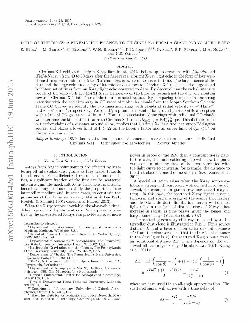
The scattering geometry of X-rays reflected by an in-terstellar dust cloud is illustrated in Fig. 1. For a sourcedistance D and a layer of interstellar dust at distancexD from the observer (such that the fractional distanceto the dust layer is x), the scattered X-rays must travelan additional distance ∆D which depends on the ob-served off-axis angle θ (e.g. Mathis & Lee 1991; Xianget al. 2011):
∆D=xD
(1
cos(θ)− 1
)+ (1− x)D
(1
cos(α)− 1
)≈ xDθ
2 + (1− x)Dα2
2=
xDθ2
2 (1− x)(1)
where we have used the small-angle approximation. Thescattered signal will arrive with a time delay of
∆t =∆D
c=
xDθ2
2c(1− x)(2)
arX
iv:1
506.
0614
2v1
[as
tro-
ph.H
E]
19
Jun
2015
2
Lig
ht ech
o / d
ust rin
g
Du
st c
lou
dDust Scattering Geometry:
θ α
θsc
xD (1–x) D
D
Fig. 1.— Cartoon of dust scattering geometry and nomenclatureused throughout this paper. X-rays from a source at distance Dscatter off a single dust layer at distance xD (such that the frac-tional distance is x). The observed angle of the scattered X-raysis θ, while the true scattering angle is θsc = θ + α. The scatteredX-rays travel an additional path length of ∆D = ∆D1 + ∆D2.
For a well-defined (short) flare of X-rays, the scatteredflare signal propagates outward from the source in anannulus of angle
θ =
√2c∆t(1− x)
xD(3)
For a point source X-ray flux F (t) scattered by a thinsheet of dust of column density NH, the X-ray intensityIν of the dust scattering annulus at angle θ observed attime tobs is given by (Mathis & Lee 1991)
Iν(θ, tobs) = NHFν(tobs −∆tθ)
(1− x)2
dσνdΩ
(4)
where ∆tθ is given by eq. (2) and dσν/dΩ is the differ-ential dust scattering cross section per Hydrogen atom,integrated over the grain size distribution (e.g. Mathis &Lee 1991; Draine 2003). In the following, we will refer tothe quantity NHdσν/dΩ as the dust scattering depth.
For a flare of finite duration scattering off a dust layerof finite thickness, the scattered signal will consist of aset of rings that reflect the different delay times for thedifferent parts of the lightcurve relative to the time of theobservation and the distribution of dust along the line ofsight.12
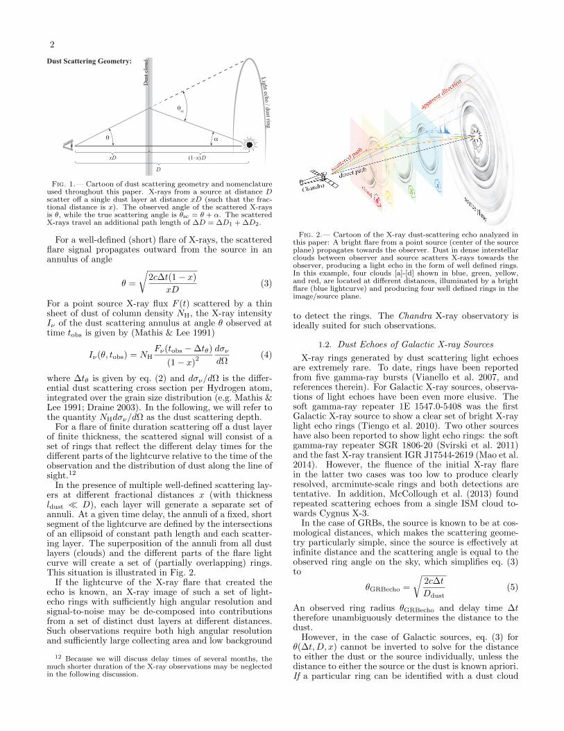
In the presence of multiple well-defined scattering lay-ers at different fractional distances x (with thicknessldust D), each layer will generate a separate set ofannuli. At a given time delay, the annuli of a fixed, shortsegment of the lightcurve are defined by the intersectionsof an ellipsoid of constant path length and each scatter-ing layer. The superposition of the annuli from all dustlayers (clouds) and the different parts of the flare lightcurve will create a set of (partially overlapping) rings.This situation is illustrated in Fig. 2.
If the lightcurve of the X-ray flare that created theecho is known, an X-ray image of such a set of light-echo rings with sufficiently high angular resolution andsignal-to-noise may be de-composed into contributionsfrom a set of distinct dust layers at different distances.Such observations require both high angular resolutionand sufficiently large collecting area and low background
12 Because we will discuss delay times of several months, themuch shorter duration of the X-ray observations may be neglectedin the following discussion.
Fig. 2.— Cartoon of the X-ray dust-scattering echo analyzed inthis paper: A bright flare from a point source (center of the sourceplane) propagates towards the observer. Dust in dense interstellarclouds between observer and source scatters X-rays towards theobserver, producing a light echo in the form of well defined rings.In this example, four clouds [a]-[d] shown in blue, green, yellow,and red, are located at different distances, illuminated by a brightflare (blue lightcurve) and producing four well defined rings in theimage/source plane.
to detect the rings. The Chandra X-ray observatory isideally suited for such observations.
1.2. Dust Echoes of Galactic X-ray Sources
X-ray rings generated by dust scattering light echoesare extremely rare. To date, rings have been reportedfrom five gamma-ray bursts (Vianello et al. 2007, andreferences therein). For Galactic X-ray sources, observa-tions of light echoes have been even more elusive. Thesoft gamma-ray repeater 1E 1547.0-5408 was the firstGalactic X-ray source to show a clear set of bright X-raylight echo rings (Tiengo et al. 2010). Two other sourceshave also been reported to show light echo rings: the softgamma-ray repeater SGR 1806-20 (Svirski et al. 2011)and the fast X-ray transient IGR J17544-2619 (Mao et al.2014). However, the fluence of the initial X-ray flarein the latter two cases was too low to produce clearlyresolved, arcminute-scale rings and both detections aretentative. In addition, McCollough et al. (2013) foundrepeated scattering echoes from a single ISM cloud to-wards Cygnus X-3.
In the case of GRBs, the source is known to be at cos-mological distances, which makes the scattering geome-try particularly simple, since the source is effectively atinfinite distance and the scattering angle is equal to theobserved ring angle on the sky, which simplifies eq. (3)to
θGRBecho =
√2c∆t
Ddust(5)
An observed ring radius θGRBecho and delay time ∆ttherefore unambiguously determines the distance to thedust.
However, in the case of Galactic sources, eq. (3) forθ(∆t,D, x) cannot be inverted to solve for the distanceto either the dust or the source individually, unless thedistance to either the source or the dust is known apriori.If a particular ring can be identified with a dust cloud
3
−100 −50 0 50t − t15801 [days]
0
1
2
3
4
5
6
2−
4 k
eV M
AX
I co
unt
rate
1 Crab
Chan
dra
ObsI
D 1
5801
Chan
dra
ObsI
D 1
6578
XM
M O
bsI
D 0
729560501
XM
M O
bsI
D 0
729560601
[XM
M O
bsI
D 0
729560701]
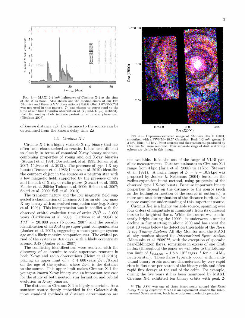
Fig. 3.— MAXI 2-4 keV lightcurve of Circinus X-1 at the timeof the 2013 flare. Also shown are the median-times of our twoChandra and three XMM observations (XMM ObsID 0729560701was not used in this paper). T0 was chosen to correspond to thetime of our first Chandra observation at (T0 =MJD15801=56683).Red diamond symbols indicate periastron at orbital phase zero(Nicolson 2007).
of known distance xD, the distance to the source can bedetermined from the known delay time ∆t.
1.3. Circinus X-1
Circinus X-1 is a highly variable X-ray binary that hasoften been characterized as erratic. It has been difficultto classify in terms of canonical X-ray binary schemes,combining properties of young and old X-ray binaries(Stewart et al. 1991; Oosterbroek et al. 1995; Jonker et al.2007; Calvelo et al. 2012). The presence of type I X-raybursts (Tennant et al. 1986; Linares et al. 2010) identifiesthe compact object in the source as a neutron star witha low magnetic field, supported by the presence of jetsand the lack of X-ray or radio pulses (Stewart et al. 1993;Fender et al. 2004a; Tudose et al. 2006; Heinz et al. 2007;Soleri et al. 2009; Sell et al. 2010).
The transient nature and the low magnetic field sug-gested a classification of Circinus X-1 as an old, low-massX-ray binary with an evolved companion star (e.g. Shireyet al. 1996). This interpretation was in conflict with the
observed orbital evolution time of order P/P ∼ 3, 000years (Parkinson et al. 2003; Clarkson et al. 2004) to
P/P ∼ 20, 000 years (Nicolson 2007) and the possibleidentification of an A-B type super-giant companion star(Jonker et al. 2007), suggesting a much younger systemage and a likely massive companion star. The orbital pe-riod of the system is 16.5 days, with a likely eccentricityaround 0.45 (Jonker et al. 2007)
The conflicting identifications were resolved with thediscovery of an arcminute scale supernova remnant inboth X-ray and radio observations (Heinz et al. 2013),placing an upper limit of τ < 4, 600 years (DCir/8 kpc)on the age of the system, where DCir is the distanceto the source. This upper limit makes Circinus X-1 theyoungest known X-ray binary and an important test casefor the study of both neutron star formation and orbitalevolution in X-ray binaries.
The distance to Circinus X-1 is highly uncertain. As asouthern source deeply embedded in the Galactic disk,most standard methods of distance determination are
Fig. 4.— Exposure-corrected image of Chandra ObsID 15801,smoothed with a FWHM=10.5” Gaussian. Red: 1-2 keV, green: 2-3 keV, blue: 3-5 keV. Point sources and the read streak produced byCircinus X-1 were removed. Four separate rings of dust scatteringechoes are visible in this image.
not available. It is also out of the range of VLBI par-allax measurements. Distance estimates to Circinus X-1range from 4 kpc (Iaria et al. 2005) to 11 kpc (Stewartet al. 1991). A likely range of D = 8 − 10.5 kpc wasproposed by Jonker & Nelemans (2004) based on theradius-expansion burst method, using properties of theobserved type I X-ray bursts. Because important binaryproperties depend on the distance to the source (suchas the Eddington fraction of the source in outburst), amore accurate determination of the distance is critical fora more complete understanding of this important source.
Circinus X-1 is a highly variable source, spanning overfour orders of magnitude in luminosity from its quiescentflux to its brightest flares. While the source was consis-tently bright during the 1990’s, it underwent a seculardecline in flux starting in about 2000 and has spent thepast 10 years below the detection thresholds of the RossiX-ray Timing Explorer All Sky Monitor and the MAXIall sky monitor aboard the International Space Station(Matsuoka et al. 2009)13, with the exception of sporadicnear-Eddington flares, sometimes in excess of one Crabin flux (throughout the paper we will refer to the Edding-ton limit of LEdd,NS ∼ 1.8 × 1038 ergs s−1 for a 1.4 Mneutron star). These flares typically occur within indi-vidual binary orbits and are characterized by very rapidrises in flux near periastron of the binary orbit and oftenrapid flux decays at the end of the orbit. For example,during the five years it has been monitored by MAXI,Circinus X-1 exhibited ten binary orbits with peak 2-
13 The ASM was one of three instruments aboard the RossiX-ray Timing Explorer; MAXI is an experiment aboard the Inter-national Space Station; both have only one mode of operation.
4
15:22:00 21:00 20:00 19:00RA (J2000)
20:00
10:00
−57:00:00
Dec (
J2000)
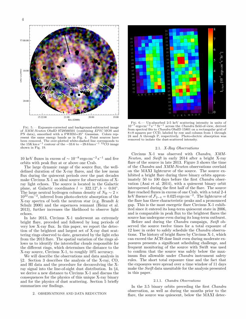
Fig. 5.— Exposure-corrected and background-subtracted imageof XMM-Newton ObsID 0729560501 (combining EPIC MOS andPN data), smoothed with a FWHM=35” Gaussian. Colors rep-resent the same energy bands as in Fig. 4. Point sources havebeen removed. The over-plotted white-dashed line corresponds tothe 15K km s−1 contour of the −33.6 to −29.6 km s−1 12CO imageshown in Fig. 19.
10 keV fluxes in excess of ∼ 10−8 ergs cm−2 s−1 and fiveorbits with peak flux at or above one Crab.
The large dynamic range of the source flux, the well-defined duration of the X-ray flares, and the low meanflux during the quiescent periods over the past decadesmake Circinus X-1 an ideal source for observations of X-ray light echoes. The source is located in the Galacticplane, at Galactic coordinates l = 322.12, b = 0.04.The large neutral hydrogen column density of NH ∼ 2×1022 cm−2, inferred from photo-electric absorption of theX-ray spectra of both the neutron star (e.g. Brandt &Schulz 2000) and the supernova remnant (Heinz et al.2013), further increases the likelihood to observe lightechoes.
In late 2013, Circinus X-1 underwent an extremelybright flare, preceded and followed by long periods ofvery low X-ray flux. In this paper, we report the detec-tion of the brightest and largest set of X-ray dust scat-tering rings observed to date, generated by the light echofrom the 2013 flare. The spatial variation of the rings al-lows us to identify the interstellar clouds responsible forthe different rings, which determines the distance to theX-ray source, Circinus X-1, to roughly 10% accuracy.
We will describe the observations and data analysis in§2. Section 3 describes the analysis of the X-ray, CO,and HI data and the procedure for deconvolving the X-ray signal into the line-of-sight dust distribution. In §4,we derive a new distance to Circinus X-1 and discuss theconsequences for the physics of this unique X-ray binaryand for the physics of dust scattering. Section 5 brieflysummarizes our findings.
2. OBSERVATIONS AND DATA REDUCTION
A B C D E F G H01
02
03
04
05
06
07
08
09
10
11
12
13
14
15
16
I J K L M N O P01
02
03
04
05
06
07
08
09
10
11
12
13
14
15
16
17
18
19
20
21
22
23
24
0
1
2
3
4
5
6
7
8
I 2−
5k
eV [
10
−7 e
rgs
cm−
2s−
1S
r−1]
Fig. 6.— Un-absorbed 2-5 keV scattering intensity in units of10−7 ergs cm−2 s−1 Sr−1 across the Chandra field-of-view, derivedfrom spectral fits to Chandra ObsID 15801 on a rectangular grid of8×8 squares per CCD, labeled by row and column from 1 through24 and A through P, respectively. Photo-electric absorption wasremoved to isolate the dust-scattered intensity.
2.1. X-Ray Observations
Circinus X-1 was observed with Chandra, XMM-Newton, and Swift in early 2014 after a bright X-rayflare of the source in late 2013. Figure 3 shows the timeof the Chandra and XMM-Newton observations overlaidon the MAXI lightcurve of the source. The source ex-hibited a bright flare during three binary orbits approx-imately 50 to 100 days before the first Chandra obser-vation (Asai et al. 2014), with a quiescent binary orbitinterspersed during the first half of the flare. The sourceflare reached fluxes in excess of one Crab, with a total 2-4keV fluence of F2−4 = 0.025 ergs cm−2. The lightcurve ofthe flare has three characteristic peaks and a pronouncedgap. This is the most energetic flare Circinus X-1 exhib-ited since it entered its long-term quiescent state in 2006,and is comparable in peak flux to the brightest flares thesource has undergone even during its long-term outburst.
Before and during the Chandra campaign, Swift ob-served the source twelve times for a total exposure of12 ksec in order to safely schedule the Chandra observa-tions. The history of bright flares by Circinus X-1, whichcan exceed the ACIS dose limit even during moderate ex-posures presents a significant scheduling challenge, andfrequent monitoring of the source with Swift was usedto confirm that the source was safely below the max-imum flux allowable under Chandra instrument safetyrules. The short total exposure time and the fact thatthe exposures were spread over a time window of 11 daysmake the Swift data unsuitable for the analysis presentedin this paper.
2.1.1. Chandra Observations
In the 3.5 binary orbits preceding the first Chandraobservation, as well as during the months prior to theflare, the source was quiescent, below the MAXI detec-
5
tion threshold. We observed the source on two occasionswith Chandra, on January 25, 2014 for 125 ksec, and onJanuary 31, 2014 for 55 ksec, listed as ObsID 15801 and16578, respectively. The point source was at very lowflux levels during both observations. Circinus X-1 wasplaced on the ACIS S3 chip.
Data were pipeline processed using CIAO software ver-sion 4.6.2. Point sources were identified using thewavdetect (Freeman et al. 2002) task and ObsID 16578was reprojected to match the astrometry of ObsID 15801.For comparison and analysis purposes, we also repro-cessed ObsID 10062 (2009) with CIAO 4.6.2 and repro-jected it to match the astrometry of ObsID 15801.
We prepared blank background images following thestandard CIAO thread (see also Hickox & Markevitch2006), matching the hard (>10 keV) X-ray spectrum ofthe background file for each chip.
Figure 4 shows an exposure-corrected, background-subtracted three-color image of the full ACIS field-ofview captured by the observation (ACIS chips 2,3,6,7,and 8 were active during the observation), where red,green, and blue correspond to the 1-2, 2-3, and 3-5 keVbands, respectively. Point sources were identified usingwavdetect in ObsIDs 10062, 15801, and 16578, sourcelists were merged and point sources were removed fromimaging and spectral analysis. The read streak was re-moved and the image was smoothed with a 10.5” full-width-half-max (FWHM) Gaussian in all three bands.
The image shows the X-ray binary point source, the X-ray jets (both over-exposed in the center of the image),and the supernova remnant in the central part of the im-age around the source position at 15:20:40.9,-57:10:00.1(J2000).
The image also clearly shows at least three bright ringsthat are concentric on the point source. The first ringspans from 4.2 to 5.7 arcminutes in radius, the secondring from 6.1 to 8.2 arcminutes, and the third from 8.3to 11.4 arcminutes in radius, predominantly covered bythe Eastern chips 2 and 3. We will refer to these ringsas rings [a], [b], and [c] from the inside out, respectively.An additional ring-like excess is visible at approximately13 arcminutes in radius, which we will refer to as ring[d].
As we will lay out in detail in §4, we interpret theserings as the dust-scattering echo from the bright flarein Oct.-Dec. of 2013, with each ring corresponding toa distinct concentration of dust along the line-of-sightto Circinus X-1. A continuous dust distribution wouldnot produce the distinct, sharp set of rings observed byChandra.
The rings are also clearly visible in ObsID 16578, de-spite the shorter exposure and the resulting lower signal-to-noise. In ObsID 16578, the rings appear at ∼4% largerradii, consistent with the expectation of a dust echo mov-ing outward in radius [see also §3.2 and eq. (10)]. Therings are easily discernible by eye in the energy bandsfrom 1 to 5 keV.
Even though the outer rings are not fully covered bythe Chandra field of view (abbreviated as FOV in thefollowing), it is clear that the rings are not uniform inbrightness as a function of azimuthal angle. There areclear intensity peaks at [15:21:00,-57:06:30] in the innerring [a] and at [15:20:20,-57:16:00] in ring [b] of ObsID15801. Generally, ring [c] appears brighter on theSouth-
A B C D E F G H01
02
03
04
05
06
07
08
09
10
11
12
13
14
15
16
I J K L M N O P01
02
03
04
05
06
07
08
09
10
11
12
13
14
15
16
17
18
19
20
21
22
23
24
1.5
1.8
2.1
2.4
2.8
3.1
3.4
3.7
4.0
N
H [
10
22 c
m−
2]
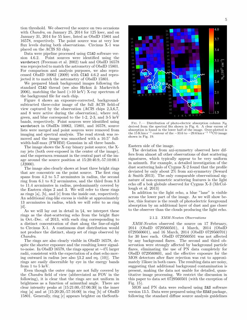
Fig. 7.— Distribution of photo-electric absorption column NHderived from the spectral fits shown in Fig. 6. A clear excess ofabsorption is found in the lower half of the image. Over-plotted isthe 15 K km s−1 contour of the −33.6 to −29.6 km s−1 12CO imageshown in Fig. 19.
Eastern side of the image.The deviation from axi-symmetry observed here dif-
fers from almost all other observations of dust scatteringsignatures, which typically appear to be very uniformin azimuth. For example, a detailed investigation of thedust scattering halo of Cygnus X-2 found that the profiledeviated by only about 2% from axi-symmetry (Seward& Smith 2013). The only comparable observational sig-nature of non-symmetric scattering features is the lightecho off a bok globule observed for Cygnus X-3 (McCol-lough et al. 2013)
In addition to the light echo, a blue ”lane” is visibleacross the lower part of the image. As we will show be-low, this feature is the result of photoelectric foregroundabsorption by an additional layer of dust and gas closerto the observer than the clouds producing the light echo.
2.1.2. XMM-Newton Observations
XMM-Newton observed the source on 17 February,2014 (ObsID 0729560501), 4 March, 2014 (ObsID0729560601), and 16 March, 2014 (ObsID 0729560701)for 30 ksec each. ObsID 0729560501 was not affectedby any background flares. The second and third ob-servation were strongly affected by background particleflares, eliminating the use of PN data completely forObsID 0729560601, and the effective exposure for theMOS detectors after flare rejection was cut to approxi-mately 15ksec in both cases. The resulting data are noisy,suggesting that additional background contamination ispresent, making the data not usable for detailed, quan-titative image processing. We restrict the discussion inthis paper to data set 0729560501 (with the exception ofFig. 15).
MOS and PN data were reduced using SAS softwareversion 13.5. Data were prepared using the ESAS package,following the standard diffuse source analysis guidelines
6
a b c
1
2
3
4
5
67
8
9
10
11
12
1.0
1.5
2.0
2.5
3.0
3.5
I 2−
5k
eV [
10
−7 e
rgs
cm−
2 s
−1 S
r−1]
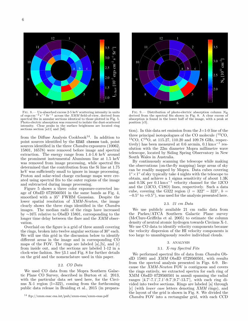
Fig. 8.— Un-absorbed excess 2-5 keV scattering intensity in unitsof ergs cm−2 s−1 Sr−1 across the XMM field-of-view, derived fromspectral fits in annular sections identical to those plotted in Fig. 5.Photo-electric absorption was removed to isolate the dust-scatteredintensity. Clear peaks in the surface brightness are located ringsections section [a11] and [b6].
from the Diffuse Analysis Cookbook14. In addition topoint sources identified by the ESAS cheese task, pointsources identified in the three Chandra exposures (10062,15801, 16578) were removed before image and spectralextraction. The energy range from 1.4-1.6 keV aroundthe prominent instrumental Aluminum line at 1.5 keVwas removed from image processing, while spectral fitsdetermined that the contribution from the Si line at 1.75keV was sufficiently small to ignore in image processing.Proton and solar-wind charge exchange maps were cre-ated using spectral fits to the outer regions of the imageand subtracted during image processing.
Figure 5 shows a three color exposure-corrected im-age of ObsID 0729560501 in the same bands as Fig. 4,smoothed with a 35” FWHM Gaussian. Despite thelower spatial resolution of XMM-Newton, the imageclearly shows the three rings identified in the Chandraimages. The median radii of the rings have increasedby ∼16% relative to ObsID 15801, corresponding to thelonger time delay between the flare and the XMM obser-vation.
Overlaid on the figure is a grid of three annuli coveringthe rings, broken into twelve angular sections of 30 each.We will use this grid in the discussion below to identifydifferent areas in the image and in corresponding COmaps of the FOV. The rings are labeled [a],[b], and [c]from inside out, and the sections are labeled 1-12 in aclock-wise fashion. See §3.1 and Fig. 8 for further detailson the grid and the nomenclature used in this paper.
2.2. CO Data
We used CO data from the Mopra Southern Galac-tic Plane CO Survey, described in Burton et al. 2013,with the particular data set used here, for the Circi-nus X-1 region (l=322), coming from the forthcomingpublic data release in Braiding et al., 2015 (in prepara-
14 ftp://xmm.esac.esa.int/pub/xmm-esas/xmm-esas.pdf
a b c
1
2
3
4
5
67
8
9
10
11
12
2.0
2.5
3.0
3.5
NH [
10
22 c
m−
2]
Fig. 9.— Distribution of photo-electric absorption column NHderived from the spectral fits shown in Fig. 8. A clear excess ofabsorption is found in the lower half of the image, with a peak atposition [c5].
tion). In this data set emission from the J=1-0 line of thethree principal isotopologues of the CO molecule (12CO,13CO, C18O, at 115.27, 110.20 and 109.78 GHz, respec-tively) has been measured at 0.6 arcmin, 0.1 km s−1 res-olution with the 22m diameter Mopra millimetre wavetelescope, located by Siding Spring Observatory in NewSouth Wales in Australia.
By continuously scanning the telescope while makingthe observations (on-the-fly mapping) large areas of skycan be readily mapped by Mopra. Data cubes covering1×1 of sky typically take 4 nights with the telescope toobtain, and achieve a 1 sigma sensitivity of about 1.3Kand 0.5K per 0.1 km s−1 velocity channel for the 12COand the (13CO, C18O) lines, respectively. Such a datacube, covering the G322 region (l = 322 − 323, b =−0.5 to +0.5), was used for the analysis presented here.
2.3. 21 cm Data
We use publicly available 21 cm radio data fromthe Parkes/ATCA Southern Galactic Plane survey(McClure-Griffiths et al. 2005) to estimate the columndensity of neutral atomic hydrogen towards Circinus X-1.We use CO data to identify velocity components becausethe velocity dispersion of the HI velocity components istoo large to unambiguously resolve individual clouds.
3. ANALYSIS
3.1. X-ray Spectral Fits
We performed spectral fits of data from Chandra Ob-sID 15801 and XMM ObsID 0729560501, with resultsfrom the spectral analysis presented in Figs. 6-9. Be-cause the XMM-Newton FOV is contiguous and coversthe rings entirely, we extracted spectra for each ring ofXMM ObsID 0729560501 in annuli spanning the radialranges [4.7’-7.1’,7.1’-9.7’,9.7’-13.7’], with each ring di-vided into twelve sections. Rings are labeled [a] through[c] (with lower case letters denoting XMM rings), andthe layout of the grid is shown in Fig. 8. We divided theChandra FOV into a rectangular grid, with each CCD
7
covered by an 8x8 grid of square apertures. The layout ofthe grid on the ACIS focal plane is shown in Fig. 6, withcolumns running from [A] through [P] and rows from 1to 24 (with capital letters denoting Chandra columns).
Spectra for Chandra ObsID 15801 were generated us-ing the specextract script after point source removal.Background spectra were generated from the blank skybackground files. No additional background model wasrequired in fitting the Chandra data, given the accuraterepresentation of the background in the black sky data.
Spectra for XMM-Newton ObsID 0729560501 were ex-tracted from the XMM-MOS data using the ESAS pack-age and following the Diffuse Analysis Cookbook. Inspectral fitting of the XMM data, we modeled instrumen-tal features (Al and Si) and solar-wind charge exchangeemission by Gaussians with line energies and intensitiestied across all spectra and line widths frozen below thespectral resolution limit of XMM-MOS at σ = 1 eV. Wemodeled the sky background emission as a sum of anabsorbed APEC model and an absorbed powerlaw. Inten-sities of both background components were tied acrossall ring sections.
We modeled the dust scattering emission in each re-gion as an absorbed powerlaw, with floating absorptioncolumn and normalization, but with powerlaw index tiedacross all regions, with the exception of the tiles cover-ing the central source and the supernova remnant in theChandra image, which span a square aperture from posi-ton [J14] to [M18]. Tying the powerlaw photon index Γacross all spectra is appropriate because (a) the scatter-ing angle varies only moderately across the rings, with
θsc =
√2c∆t
(1− x)xD(6)
and (b) for the scattering angles considered here (θsc >10′), the energy dependence of the scattering cross sec-tion is independent of θsc, with dσ/dΩ ∝ E−2 (e.g.Draine 2003). While the source spectrum might havevaried during the outburst, we are integrating over suffi-ciently large apertures to average over possible spectralvariations.
While the source spectrum during outburst (the echoof which we are observing in the rings) was likely morecomplicated than a simple powerlaw, we have no directmeasurement of the detailed flare spectrum and the qual-ity of the spectra does not warrant additional complica-tions, such as the addition of emission lines which areoften present in the spectra when the source is bright(Brandt & Schulz 2000). Dust scattering is expected tosteepen the source spectrum by ∆Γ = 2, and the mea-sured powerlaw index of
Γ = 4.00± 0.03 (7)
for the scattered emission is consistent with the typicallysoft spectrum of Γ ∼ 2 the source displays when in out-burst.
The spectral fits resulting from the model are sta-tistically satisfactory, with a reduced chisquare ofχ2
red,0729560501 = 839.68/807 d.o.f. = 1.04 for the com-bined fit of the entire set of spectra for ObsID 0729560501and χ2
red,15801 = 839.68/807 d.o.f. = 1.05 for ObsID
4 6 8 10 12 14 16θ [arcmin]
0
1•10−7
2•10−7
3•10−7
I2−
5keV
[er
gs
cm−
2 s
−1 S
r−1]
[a]
[b]
[c]
[d]
sum
θ/θmed
K2
−5
keV
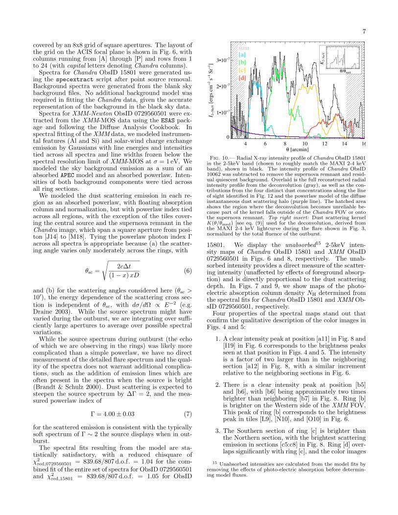
Fig. 10.— Radial X-ray intensity profile of Chandra ObsID 15801in the 2-5keV band (chosen to roughly match the MAXI 2-4 keVband), shown in black. The intensity profile of Chandra ObsID10062 was subtracted to remove the supernova remnant and resid-ual quiescent background. Overlaid is the full reconstructed radialintensity profile from the deconvolution (gray), as well as the con-tributions from the four distinct dust concentrations along the lineof sight identified in Fig. 12 and the powerlaw model of the diffuseinstantaneous dust scattering halo (purple line). The hatched areashows the region where the deconvolution becomes unreliable be-cause part of the kernel falls outside of the Chandra FOV or ontothe supernova remnant. Top right insert: Dust scattering kernelK(θ/θmed) [see eq. (9)] used for the deconvolution, derived fromthe MAXI 2-4 keV lightcurve during the flare shown in Fig. 3,normalized by the total fluence of the outburst.
15801. We display the unabsorbed15 2-5keV inten-sity maps of Chandra ObsID 15801 and XMM ObsID0729560501 in Figs. 6 and 8, respectively. The unab-sorbed intensity provides a direct measure of the scatter-ing intensity (unaffected by effects of foreground absorp-tion) and is directly proportional to the dust scatteringdepth. In Figs. 7 and 9, we show maps of the photo-electric absorption column density NH determined fromthe spectral fits for Chandra ObsID 15801 and XMM Ob-sID 0729560501, respectively.
Four properties of the spectral maps stand out thatconfirm the qualitative description of the color images inFigs. 4 and 5:
1. A clear intensity peak at position [a11] in Fig. 8 and[I19] in Fig. 6 corresponds to the brightness peaksseen at that position in Figs. 4 and 5. The intensityis a factor of two larger than in the neighboringsection [a12] in Fig. 8, with a similar incrementrelative to the neighboring sections in Fig. 6.
2. There is a clear intensity peak at position [b5]and [b6], with [b6] being approximately two timesbrighter than neighboring [b7] in Fig. 8. Ring [b]is brighter on the Western side of the XMM FOV.This peak of ring [b] corresponds to the brightnesspeak in tiles [L9], [N10], and [O10] in Fig. 6.
3. The Southern section of ring [c] is brighter thanthe Northern section, with the brightest scatteringemission in sections [c5:c8] in Fig. 8. Ring [d] over-laps significantly with ring [c], and the color images
15 Unabsorbed intensities are calculated from the model fits byremoving the effects of photo-electric absorption before determin-ing model fluxes.
8
and intensity maps cannot distinguish the angulardistribution of the two rings.
4. There is a clear excess of foreground absorption inthe Southern sections of the FOV, running fromtile [P7] to [B6] in Fig. 7. Figure 9 shows thestrongest absorption in sections [c5], [b6] and [b7].This corresponds to the blue absorption lane thatruns across the color images in Figs. 4 and 5.
The rings clearly deviate from axial symmetry aboutCircinus X-1, which requires a strong variation in thescattering dust column density across the image. Be-cause the rings are well-defined, sharp features, each ringrequires the presence of a spatially well separated, thindistribution of dust (where thin means that the extentof the dust sheet responsible for each ring is significantlysmaller than the distance to the source, by at least anorder of magnitude).
We present a quantitative analysis of the dust distri-bution derived from the rings in 3.2, but from simpleconsideration of the images and spectral maps alone, itis clear that the different dust clouds responsible for therings have different spatial distributions and cannot beuniform across the XMM and Chandra FOVs. In partic-ular, the peak of the cloud that produced the innermostring (ring [a]) must have a strong column density peakin section [a11], while the cloud producing ring [b] mustshow a strong peak in sections [b5] and [b6]. The ex-cess of photo-electric absorption in the lower half of theimage, with a lane of absorption running through thesections [c5], [b6], and [b7], requires a significant amountof foreground dust and gas (an excess column of approx-imately NH ∼ 1022 cm−2 relative to the rest of the field).
3.2. X-ray Intensity Profiles and Dust Distributions
3.2.1. Radial intensity profiles
In order to determine quantitatively the dust distribu-tion along the line of sight, we extracted radial intensityprofiles of Chandra ObsID 10062, 15801, and 16578 in600 logarithmic radial bins from 1’ to 18’.5 in the energybands 1-2 keV, 2-3 keV, and 3-5 keV (after backgroundsubtraction and point-source/read-streak removal). Weextracted the radial profile of XMM ObsID 0729560501in 300 logarithmic bins over the same range in angles.We subtracted the quiescent radial intensity profile ofObsID 10062 to remove the emission by the supernovaremnant and residual background emission.
Because of the variation in photo-electric absorptionacross the field, we restricted analysis to the 2-5 keVband, which is only moderately affected by absorption.We plot the resulting radial intensity profile of ChandraObsID 15801 in Fig. 10. The plot in Fig. 10 shows fourecho rings labeled [a] through [d] which correspond to thevisually identified rings in the previous sections. Severalbright sharp peaks in I2−5keV(θ) are visible that can alsobe seen as distinct sharp rings in Fig. 4, suggesting verylocalized dust concentrations. For comparison, the radialprofile of XMM ObsID 0729560501 is plotted in Fig. 11.
3.2.2. Modeling and removing the diffuse instantaneous dustscattering halo
In general, the dust scattering ring echo will be super-imposed on the lower-level instantaneous diffuse dust
4 6 8 10 12 14 16θ [arcmin]
0
5.0•10−8
1.0•10−7
1.5•10−7
2.0•10−7
2.5•10−7
I2−
5keV
[er
gs
cm s
Sr
]
θ/θmed
K2
−5
keV
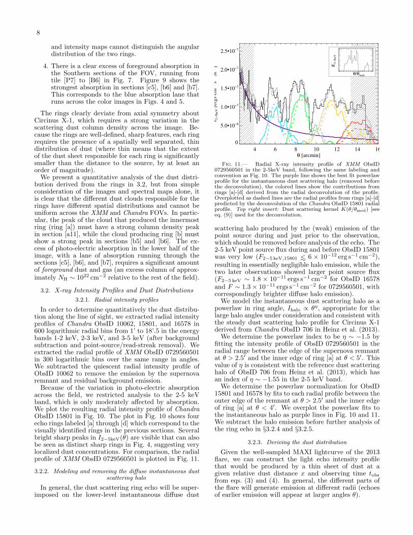
Fig. 11.— Radial X-ray intensity profile of XMM ObsID0729560501 in the 2-5keV band, following the same labeling andconvention as Fig. 10. The purple line shows the best fit powerlawprofile for the instantaneous dust scattering halo (removed beforethe deconvolution), the colored lines show the contributions fromrings [a]-[d] derived from the radial deconvolution of the profile.Overplotted as dashed lines are the radial profiles from rings [a]-[d]predicted by the deconvolution of the Chandra ObsID 15801 radialprofile. Top right insert: Dust scattering kernel K(θ/θmed) [seeeq. (9)] used for the deconvolution.
scattering halo produced by the (weak) emission of thepoint source during and just prior to the observation,which should be removed before analysis of the echo. The2-5 keV point source flux during and before ObsID 15801was very low (F2−5 keV,15801 ∼< 6 × 10⁻¹² erg s−1 cm−2),resulting in essentially negligible halo emission, while thetwo later observations showed larger point source flux(F2−5 keV ∼ 1.8 × 10⁻¹¹ ergs s−1 cm−2 for ObsID 16578and F ∼ 1.3× 10⁻¹¹ ergs s−1 cm−2 for 0729560501, withcorrespondingly brighter diffuse halo emission).
We model the instantaneous dust scattering halo as apowerlaw in ring angle, Ihalo ∝ θη, appropriate for thelarge halo angles under consideration and consistent withthe steady dust scattering halo profile for Circinus X-1derived from Chandra ObsID 706 in Heinz et al. (2013).
We determine the powerlaw index to be η ∼ −1.5 byfitting the intensity profile of ObsID 0729560501 in theradial range between the edge of the supernova remnantat θ > 2.5′ and the inner edge of ring [a] at θ < 5′. Thisvalue of η is consistent with the reference dust scatteringhalo of ObsID 706 from Heinz et al. (2013), which hasan index of η ∼ −1.55 in the 2-5 keV band.
We determine the powerlaw normalization for ObsID15801 and 16578 by fits to each radial profile between theouter edge of the remnant at θ > 2.5′ and the inner edgeof ring [a] at θ < 4′. We overplot the powerlaw fits tothe instantaneous halo as purple lines in Fig. 10 and 11.We subtract the halo emission before further analysis ofthe ring echo in §3.2.4 and §3.2.5.
3.2.3. Deriving the dust distribution
Given the well-sampled MAXI lightcurve of the 2013flare, we can construct the light echo intensity profilethat would be produced by a thin sheet of dust at agiven relative dust distance x and observing time tobs
from eqs. (3) and (4). In general, the different parts ofthe flare will generate emission at different radii (echoesof earlier emission will appear at larger angles θ).
9
The scattering angle and thus the scattering cross sec-tion will vary for different parts of the lightcurve, whichmust be modeled. Given the large scattering angles ofθsc ∼> 1400′′ of the rings and photon energies above 2keV, it is safe to assume that the cross section is in thelarge angle limit where dσ/dΩ ∝ θ−αsc ∝ θ−α with α ∼ 4(Draine 2003), which we will use in the following. Theexact value of α depends on the unknown grain size dis-tribution. By repeating the analysis process with differ-ent values of α, ranging from 3 to 5, we have verified thatour results (in particular, the location of the dust cloudsand the distance to Circinus X-1) are not sensitive to theexact value of α.
For a thin scattering sheet at fractional distance x, themedian ring angle θmed (i.e., the observed angle θ for themedian time delay ∆tmed of the flare) is
θmed =
√2c∆tmed(1− x)
xD(8)
where ∆tmed is a constant set only by the date of theobservation and the date range of the flare. The invariantintensity profile K2−5keV produced by that sheet dependson the observed angle θ only through the dimensionlessratio z ≡ θ/θmed:
K2−5keV (z, x)
=FMAXI(∆tmedz2)
NH,x
(1− x)2
dσ
dΩ
∣∣∣∣θ=θmed
z−4 (9)
We can therefore decompose the observed radial profileinto a series of these contributions from scattering sheetsalong the line of sight, each of the form K2−5keV(θ/θmed).Because we chose logarithmic radial bins for the intensityprofile, we can achieve this by a simple deconvolution ofI2−5keV with the kernel K2−5keV. The inset in Fig. 10shows K(θ/θmed) for α = 4.
3.2.4. Deconvolution of the Chandra radial profiles
To derive the dust distribution that gave rise to thelight echo, we performed a maximum likelihood decon-volution of the Chandra radial profiles with this kernelinto a set of 600 dust scattering screens along the lineof sight. We used the Lucy-Richardson deconvolution al-gorithm (Richardson 1972; Lucy 1974) implemented inthe IDL ASTROLIB library16. In the region of interest(where the scattering profile is not affected by the chipedge and the supernova remnant), the radial bins arelarger than the 50% enclosed energy width of the Chan-dra point spread function (PSF), such that the emissioninside each radial bin is resolved17.
Figure 10 shows the reconstructed intensity profilefrom this distribution for ObsID 15801 (derived by re-convolving the deconvolution with K2−5 keV and addingit to the powerlaw profile for the instantaneous dust scat-tering halo), which reproduces the observed intensityprofile very well, with only minor deviations primarily
16 http://idlastro.gsfc.nasa.gov/ftp/pro/image/max likelihood.pro17 We verified that our results are robust against PSF effects by
repeating the deconvolution after smoothing both the profile andthe kernel with Gaussians of equal width; this mimicks the effectsPSF smearing would have on the deconvolution. The smoothingdoes not affect our results significantly even for widths an order ofmagnitude larger than the Chandra PSF.
4 6 8 10 12 14 16θ [arcmin]
0
5
10
15
20
(1−
x)−
2 N
H d
σ/d
Ω [
Sr−
1]
0
1
2
3
NH d
σ/d
Ω [
Sr−
1]
[a] [b] [c] [d]
4 6 8
Ddust [kpc]
−70 −75.3 −70 −60 −50
Radial Velocity VLSR [km s−1]
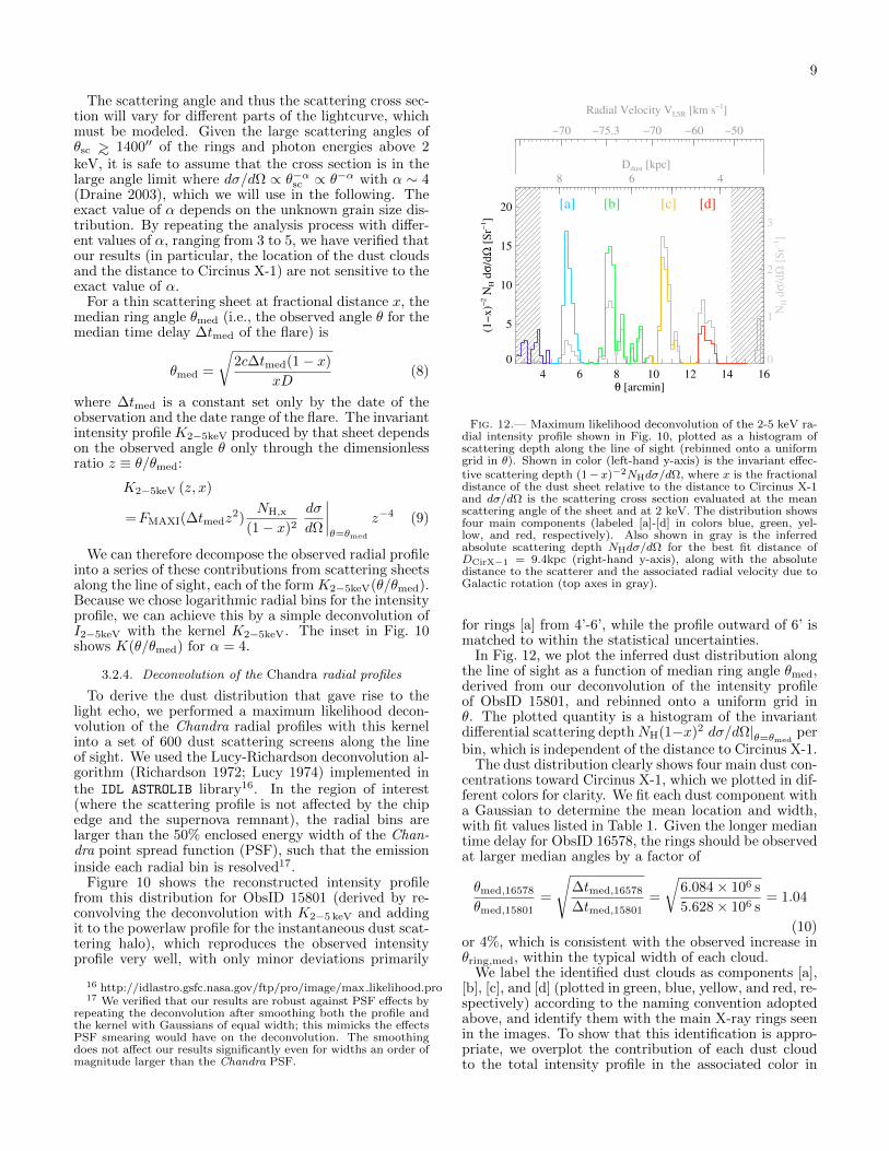
Fig. 12.— Maximum likelihood deconvolution of the 2-5 keV ra-dial intensity profile shown in Fig. 10, plotted as a histogram ofscattering depth along the line of sight (rebinned onto a uniformgrid in θ). Shown in color (left-hand y-axis) is the invariant effec-tive scattering depth (1−x)−2NHdσ/dΩ, where x is the fractionaldistance of the dust sheet relative to the distance to Circinus X-1and dσ/dΩ is the scattering cross section evaluated at the meanscattering angle of the sheet and at 2 keV. The distribution showsfour main components (labeled [a]-[d] in colors blue, green, yel-low, and red, respectively). Also shown in gray is the inferredabsolute scattering depth NHdσ/dΩ for the best fit distance ofDCirX−1 = 9.4kpc (right-hand y-axis), along with the absolutedistance to the scatterer and the associated radial velocity due toGalactic rotation (top axes in gray).
for rings [a] from 4’-6’, while the profile outward of 6’ ismatched to within the statistical uncertainties.
In Fig. 12, we plot the inferred dust distribution alongthe line of sight as a function of median ring angle θmed,derived from our deconvolution of the intensity profileof ObsID 15801, and rebinned onto a uniform grid inθ. The plotted quantity is a histogram of the invariantdifferential scattering depth NH(1−x)2 dσ/dΩ|θ=θmed
perbin, which is independent of the distance to Circinus X-1.
The dust distribution clearly shows four main dust con-centrations toward Circinus X-1, which we plotted in dif-ferent colors for clarity. We fit each dust component witha Gaussian to determine the mean location and width,with fit values listed in Table 1. Given the longer mediantime delay for ObsID 16578, the rings should be observedat larger median angles by a factor of
θmed,16578
θmed,15801=
√∆tmed,16578
∆tmed,15801=
√6.084× 10⁶ s
5.628× 10⁶ s= 1.04
(10)or 4%, which is consistent with the observed increase inθring,med, within the typical width of each cloud.
We label the identified dust clouds as components [a],[b], [c], and [d] (plotted in green, blue, yellow, and red, re-spectively) according to the naming convention adoptedabove, and identify them with the main X-ray rings seenin the images. To show that this identification is appro-priate, we overplot the contribution of each dust cloudto the total intensity profile in the associated color in
10
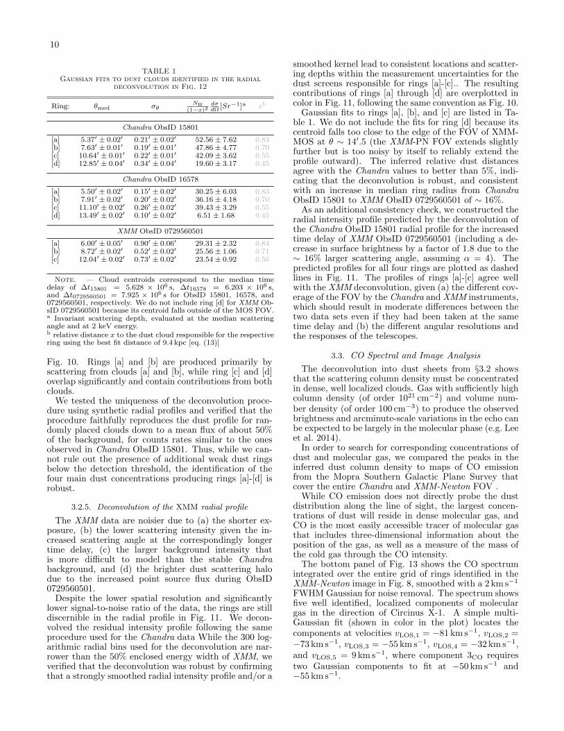
TABLE 1Gaussian fits to dust clouds identified in the radial
deconvolution in Fig. 12
Ring: θmed σθNH
(1−x)2dσdΩ
[Sr−1]a xb
Chandra ObsID 15801
[a] 5.37′ ± 0.02′ 0.21′ ± 0.02′ 52.56 ± 7.62 0.83[b] 7.63′ ± 0.01′ 0.19′ ± 0.01′ 47.86 ± 4.77 0.70[c] 10.64′ ± 0.01′ 0.22′ ± 0.01′ 42.09 ± 3.62 0.55[d] 12.85′ ± 0.04′ 0.34′ ± 0.04′ 19.60 ± 3.17 0.45
Chandra ObsID 16578
[a] 5.50′ ± 0.02′ 0.15′ ± 0.02′ 30.25 ± 6.03 0.83[b] 7.91′ ± 0.02′ 0.20′ ± 0.02′ 36.16 ± 4.18 0.70[c] 11.10′ ± 0.02′ 0.26′ ± 0.02′ 39.43 ± 3.29 0.55[d] 13.49′ ± 0.02′ 0.10′ ± 0.02′ 6.51 ± 1.68 0.45
XMM ObsID 0729560501
[a] 6.00′ ± 0.05′ 0.90′ ± 0.06′ 29.31 ± 2.32 0.84[b] 8.72′ ± 0.02′ 0.52′ ± 0.02′ 25.56 ± 1.06 0.71[c] 12.04′ ± 0.02′ 0.73′ ± 0.02′ 23.54 ± 0.92 0.56
Note. — Cloud centroids correspond to the median timedelay of ∆t15801 = 5.628 × 10⁶ s, ∆t16578 = 6.203 × 10⁶ s,and ∆t0729560501 = 7.925 × 10⁶ s for ObsID 15801, 16578, and0729560501, respectively. We do not include ring [d] for XMM Ob-sID 0729560501 because its centroid falls outside of the MOS FOV.a Invariant scattering depth, evaluated at the median scatteringangle and at 2 keV energy.b relative distance x to the dust cloud responsible for the respectivering using the best fit distance of 9.4 kpc [eq. (13)]
Fig. 10. Rings [a] and [b] are produced primarily byscattering from clouds [a] and [b], while ring [c] and [d]overlap significantly and contain contributions from bothclouds.
We tested the uniqueness of the deconvolution proce-dure using synthetic radial profiles and verified that theprocedure faithfully reproduces the dust profile for ran-domly placed clouds down to a mean flux of about 50%of the background, for counts rates similar to the onesobserved in Chandra ObsID 15801. Thus, while we can-not rule out the presence of additional weak dust ringsbelow the detection threshold, the identification of thefour main dust concentrations producing rings [a]-[d] isrobust.
3.2.5. Deconvolution of the XMM radial profile
The XMM data are noisier due to (a) the shorter ex-posure, (b) the lower scattering intensity given the in-creased scattering angle at the correspondingly longertime delay, (c) the larger background intensity thatis more difficult to model than the stable Chandrabackground, and (d) the brighter dust scattering halodue to the increased point source flux during ObsID0729560501.
Despite the lower spatial resolution and significantlylower signal-to-noise ratio of the data, the rings are stilldiscernible in the radial profile in Fig. 11. We decon-volved the residual intensity profile following the sameprocedure used for the Chandra data While the 300 log-arithmic radial bins used for the deconvolution are nar-rower than the 50% enclosed energy width of XMM, weverified that the deconvolution was robust by confirmingthat a strongly smoothed radial intensity profile and/or a
smoothed kernel lead to consistent locations and scatter-ing depths within the measurement uncertainties for thedust screens responsible for rings [a]-[c].. The resultingcontributions of rings [a] through [d] are overplotted incolor in Fig. 11, following the same convention as Fig. 10.
Gaussian fits to rings [a], [b], and [c] are listed in Ta-ble 1. We do not include the fits for ring [d] because itscentroid falls too close to the edge of the FOV of XMM-MOS at θ ∼ 14′.5 (the XMM-PN FOV extends slightlyfurther but is too noisy by itself to reliably extend theprofile outward). The inferred relative dust distancesagree with the Chandra values to better than 5%, indi-cating that the deconvolution is robust, and consistentwith an increase in median ring radius from ChandraObsID 15801 to XMM ObsID 0729560501 of ∼ 16%.
As an additional consistency check, we constructed theradial intensity profile predicted by the deconvolution ofthe Chandra ObsID 15801 radial profile for the increasedtime delay of XMM ObsID 0729560501 (including a de-crease in surface brightness by a factor of 1.8 due to the∼ 16% larger scattering angle, assuming α = 4). Thepredicted profiles for all four rings are plotted as dashedlines in Fig. 11. The profiles of rings [a]-[c] agree wellwith the XMM deconvolution, given (a) the different cov-erage of the FOV by the Chandra and XMM instruments,which should result in moderate differences between thetwo data sets even if they had been taken at the sametime delay and (b) the different angular resolutions andthe responses of the telescopes.
3.3. CO Spectral and Image Analysis
The deconvolution into dust sheets from §3.2 showsthat the scattering column density must be concentratedin dense, well localized clouds. Gas with sufficiently highcolumn density (of order 1021 cm−2) and volume num-ber density (of order 100 cm−3) to produce the observedbrightness and arcminute-scale variations in the echo canbe expected to be largely in the molecular phase (e.g. Leeet al. 2014).
In order to search for corresponding concentrations ofdust and molecular gas, we compared the peaks in theinferred dust column density to maps of CO emissionfrom the Mopra Southern Galactic Plane Survey thatcover the entire Chandra and XMM-Newton FOV .
While CO emission does not directly probe the dustdistribution along the line of sight, the largest concen-trations of dust will reside in dense molecular gas, andCO is the most easily accessible tracer of molecular gasthat includes three-dimensional information about theposition of the gas, as well as a measure of the mass ofthe cold gas through the CO intensity.
The bottom panel of Fig. 13 shows the CO spectrumintegrated over the entire grid of rings identified in theXMM-Newton image in Fig. 8, smoothed with a 2 km s−1
FWHM Gaussian for noise removal. The spectrum showsfive well identified, localized components of moleculargas in the direction of Circinus X-1. A simple multi-Gaussian fit (shown in color in the plot) locates thecomponents at velocities vLOS,1 = −81 km s−1, vLOS,2 =−73 km s−1, vLOS,3 = −55 km s−1, vLOS,4 = −32 km s−1,and vLOS,5 = 9 km s−1, where component 3CO requirestwo Gaussian components to fit at −50 km s−1 and−55 km s−1.
11
−80 −60 −40 −20 0Radial Velocity VLSR [km s−1]
0.0
0.5
1.0
1.5
2.0
2.5
3.0
T12C
O [
K]
1CO
2CO 3CO
4CO
5CO
0
20
40
60
80
100
TH
I [K
]
1HI 2HI 3HI 4HI 5HI
2
4
6
8
10
12
14D
[kpc]
l=322.12, b=0
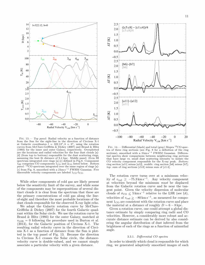
Fig. 13.— Top panel: Radial velocity as a function of distancefrom the Sun for the sight-line in the direction of Circinus X-1at Galactic coordinates l = 322.12, b = 0, using the rotationcurves from McClure-Griffiths & Dickey (2007) and Brand & Blitz(1993) for the inner and outer Galaxy, respectively. Overplottedare the locations and radial velocities for the four dust clouds [a]-[d] (from top to bottom) responsible for the dust scattering rings,assuming the best fit distance of 9.4 kpc. Middle panel: 21cm HIspectrum integrated over rings [a]-[c] defined in Fig.8. Component1HI comprises CO components 1CO and 2CO listed below. Bottompanel: 12CO spectrum integrated over the same region of rings [a]-[c] from Fig. 8, smoothed with a 2 km s−1 FWHM Gaussian. Fivediscernible velocity components are labeled 1CO-5CO.
While other components of cold gas are likely presentbelow the sensitivity limit of the survey, and while someof the components may be superpositions of several dis-tinct clouds it is clear from the spectrum that these arethe primary concentrations of cold gas along the line-of-sight and therefore the most probable locations of thedust clouds responsible for the observed X-ray light echo.
We adopt the Galactic rotation curve by McClure-Griffiths & Dickey (2007) for the fourth Galactic quad-rant within the Solar circle. We use the rotation curve byBrand & Blitz (1993) for the outer Galaxy, matched atvLSR = 0 following the procedure used in Burton et al.(2013), for the Galactic position of Circinus X-1. Theresulting radial velocity curve in the direction of Circi-nus X-1 as a function of distance from the Sun is plot-ted in the top panel of Fig. 13. Because the directionto Circinus X-1 crosses the Solar circle, the distance-velocity curve is double-valued, and we cannot simplyassociate a particular velocity with a given distance.
−100 −80 −60 −40 −20 0 20Radial Velocity VLSR [km s−1]
−0.5
0.0
0.5
1.0
1.5
2.0
2.5
∆T
[K
]
[a11]−[a12][a11]
−0.5
0.0
0.5
1.0
1.5
2.0
2.5
∆T
[K
]
[b6]−[b7][b6]
−0.5
0.0
0.5
1.0
1.5
2.0
2.5
∆T
[K
]
([c5:c8] − [c1:c4])/4[c5:c8]/4
Fig. 14.— Differential (black) and total (gray) Mopra 12CO spec-tra of three ring sections (see Fig. 8 for a definition of the ringsections), smoothed with a 3 km s−1 FWHM Gaussian. Differen-tial spectra show comparisons between neighboring ring sectionsthat have large vs. small dust scattering intensity to isolate theCO velocity component responsible for the X-ray peak. Bottom:ring section [a11] minus [a12], middle: ring section [b6] minus [b7];top: sum of ring sections [c5:8] minus sum of [c1:4].
The rotation curve turns over at a minimum veloc-ity of vrad ≥ −75.3 km s−1. Any velocity componentat velocities beyond the minimum must be displacedfrom the Galactic rotation curve and lie near the tan-gent point. Given the velocity dispersion of molecularclouds of σCO ∼< 5 km s−1 relative to the LSR (see §4),
velocities of vrad ∼> −80 km s−1, as measured for compo-nent 1CO are consistent with the rotation curve and placethe material at a distance of roughly D ∼ 6− 8 kpc.
Given a rotation curve, one could attempt a global dis-tance estimate by simply comparing ring radii and COvelocities. However, a considerably more robust and ac-curate distance estimate can be derived by also consid-ering the angular distribution of dust inferred from thebrightness of each of the rings as a function of azimuthalangle.
3.3.1. Differential CO spectra
In order to identify which cloud is responsible for whichring, we generated adaptively smoothed images of each
12
0
2
4
6
8
K k
m s
−1
15:22:00 21:00 20:00 19:00
RA (J2000)
20:00
10:00
−57:00:00
Dec (
J2000)
−76.0 to −72.0 km/s
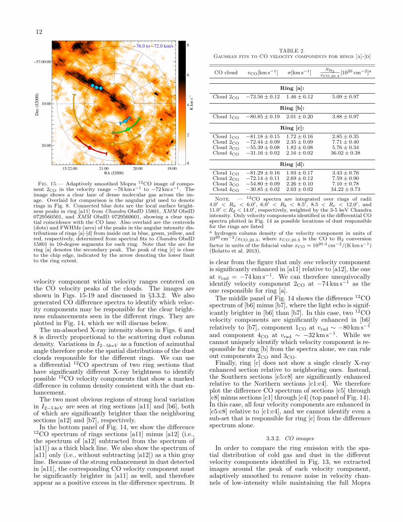
Fig. 15.— Adaptively smoothed Mopra 12CO image of compo-nent 2CO in the velocity range −76 km s−1 to −72 km s−1. Theimage shows a clear lane of dense molecular gas across the im-age. Overlaid for comparison is the angular grid used to denoterings in Fig. 8. Connected blue dots are the local surface bright-ness peaks in ring [a11] from Chandra ObsID 15801, XMM ObsID0729560501, and XMM ObsID 0729560601, showing a clear spa-tial coincidence with the CO lane. Also overlaid are the centroids(dots) and FWHMs (arcs) of the peaks in the angular intensity dis-tributions of rings [a]-[d] from inside out in blue, green, yellow, andred, respectively, determined from spectral fits to Chandra ObsID15801 in 10-degree segments for each ring. Note that the arc forring [a] denotes the secondary peak. The peak of ring [c] is closeto the chip edge, indicated by the arrow denoting the lower limitto the ring extent.
velocity component within velocity ranges centered onthe CO velocity peaks of the clouds. The images areshown in Figs. 15-19 and discussed in §3.3.2. We alsogenerated CO difference spectra to identify which veloc-ity components may be responsible for the clear bright-ness enhancements seen in the different rings. They areplotted in Fig. 14, which we will discuss below.
The un-absorbed X-ray intensity shown in Figs. 6 and8 is directly proportional to the scattering dust columndensity. Variations in I2−5keV as a function of azimuthalangle therefore probe the spatial distributions of the dustclouds responsible for the different rings. We can usea differential 12CO spectrum of two ring sections thathave significantly different X-ray brightness to identifypossible 12CO velocity components that show a markeddifference in column density consistent with the dust en-hancement.
The two most obvious regions of strong local variationin I2−5 keV are seen at ring sections [a11] and [b6], bothof which are significantly brighter than the neighboringsections [a12] and [b7], respectively.
In the bottom panel of Fig. 14, we show the difference12CO spectrum of rings sections [a11] minus [a12] (i.e.,the spectrum of [a12] subtracted from the spectrum of[a11]) as a thick black line. We also show the spectrum of[a11] only (i.e., without subtracting [a12]) as a thin grayline. Because of the strong enhancement in dust detectedin [a11], the corresponding CO velocity component mustbe significantly brighter in [a11] as well, and thereforeappear as a positive excess in the difference spectrum. It
TABLE 2Gaussian fits to CO velocity components for rings [a]-[d]
CO cloud vCO[km s−1] σ[km s−1]NH2
xCO,20.3[1020 cm−2]a
Ring [a]:
Cloud 2CO −73.56 ± 0.12 1.46 ± 0.12 5.09 ± 0.97
Ring [b]:
Cloud 1CO −80.85 ± 0.19 2.01 ± 0.20 3.88 ± 0.97
Ring [c]:
Cloud 1CO −81.18 ± 0.15 1.72 ± 0.16 2.85 ± 0.35Cloud 2CO −72.44 ± 0.09 2.35 ± 0.09 7.71 ± 0.40Cloud 3CO −55.39 ± 0.08 1.82 ± 0.08 5.76 ± 0.34Cloud 4CO −31.16 ± 0.02 2.16 ± 0.02 36.02 ± 0.38
Ring [d]:
Cloud 1CO −81.29 ± 0.16 1.93 ± 0.17 3.43 ± 0.76Cloud 2CO −72.14 ± 0.11 2.69 ± 0.12 7.59 ± 0.90Cloud 3CO −54.80 ± 0.09 2.26 ± 0.10 7.10 ± 0.78Cloud 4CO −30.85 ± 0.02 2.03 ± 0.02 34.22 ± 0.73
Note. — 12CO spectra are integrated over rings of radii4.0′ < Ra < 6.0′, 6.0′ < Rb < 8.5′, 8.5 < Rc < 12.0′, and11.0′ < Rd < 14.0′, respectively, weighted by the 3-5 keV Chandraintensity. Only velocity components identified in the differential COspectra plotted in Fig. 14 as possible locations of dust responsiblefor the rings are listeda hydrogen column density of the velocity component in units of1020 cm−2/xCO,20.3, where xCO,20.3 is the CO to H2 conversion
factor in units of the fiducial value xCO = 1020.3 cm−2/(K km s−1)(Bolatto et al. 2013).
is clear from the figure that only one velocity componentis significantly enhanced in [a11] relative to [a12], the oneat vrad = −74 km s−1. We can therefore unequivocallyidentify velocity component 2CO at −74 km s−1 as theone responsible for ring [a].
The middle panel of Fig. 14 shows the difference 12COspectrum of [b6] minus [b7], where the light echo is signif-icantly brighter in [b6] than [b7]. In this case, two 12COvelocity components are significantly enhanced in [b6]relatively to [b7], component 1CO at vrad ∼ −80 km s−1
and component 4CO at vrad ∼ −32 km s−1. While wecannot uniquely identify which velocity component is re-sponsible for ring [b] from the spectra alone, we can ruleout components 2CO and 3CO.
Finally, ring [c] does not show a single clearly X-rayenhanced section relative to neighboring ones. Instead,the Southern sections [c5:c8] are significantly enhancedrelative to the Northern sections [c1:c4]. We thereforeplot the difference CO spectrum of sections [c5] through[c8] minus sections [c1] through [c4] (top panel of Fig. 14).In this case, all four velocity components are enhanced in[c5:c8] relative to [c1:c4], and we cannot identify even asub-set that is responsible for ring [c] from the differencespectrum alone.
3.3.2. CO images
In order to compare the ring emission with the spa-tial distribution of cold gas and dust in the differentvelocity components identified in Fig. 13, we extractedimages around the peak of each velocity component,adaptively smoothed to remove noise in velocity chan-nels of low-intensity while maintaining the full Mopra
13
0
2
4
6
8
10
K k
m s
−1
15:22:00 21:00 20:00 19:00
RA (J2000)
20:00
10:00
−57:00:00
Dec (
J2000)
−85.0 to −75.0 km/s
Fig. 16.— Adaptively smoothed Mopra 12CO image of compo-nent 1CO in the velocity range −85 km s−1 to −75 km s−1, samenomenclature as in Fig. 15. The CO emission in this band showsa clear peak at locations [b5] and [b6], matching the intensity dis-tribution of X-ray ring [b] (green ring segment).
angular resolution in bright velocity channels. We em-ployed a Gaussian spatial smoothing kernel with widthσ = 1.5′ × [1.0 − 0.9 exp[−(v − vpeak)/(2σ2
CO)], wherevpeak and σCO are the peak velocity and the dispersionof Gaussian fits to the summed CO spectra shown inFig. 14. This prescription was chosen heuristically toproduce sharp yet low-noise images of the different COclouds.
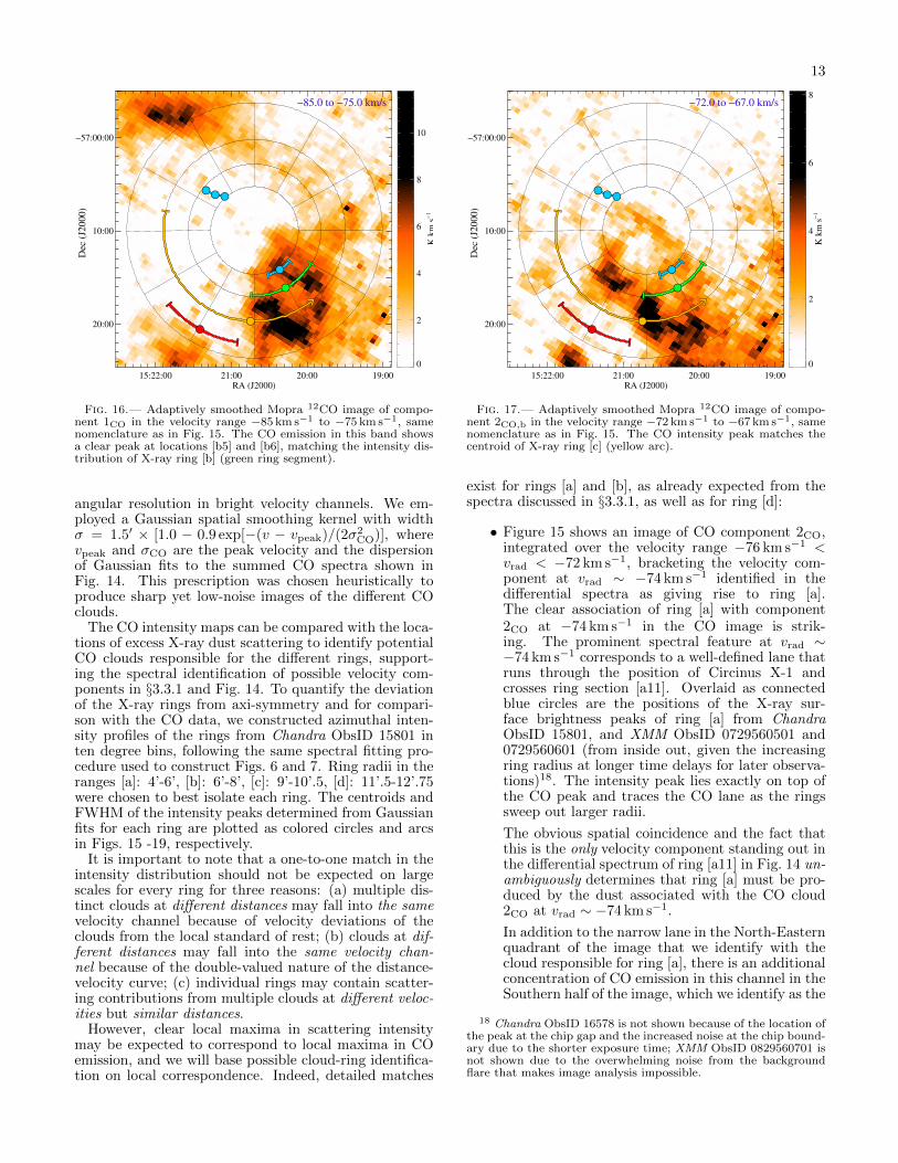
The CO intensity maps can be compared with the loca-tions of excess X-ray dust scattering to identify potentialCO clouds responsible for the different rings, support-ing the spectral identification of possible velocity com-ponents in §3.3.1 and Fig. 14. To quantify the deviationof the X-ray rings from axi-symmetry and for compari-son with the CO data, we constructed azimuthal inten-sity profiles of the rings from Chandra ObsID 15801 inten degree bins, following the same spectral fitting pro-cedure used to construct Figs. 6 and 7. Ring radii in theranges [a]: 4’-6’, [b]: 6’-8’, [c]: 9’-10’.5, [d]: 11’.5-12’.75were chosen to best isolate each ring. The centroids andFWHM of the intensity peaks determined from Gaussianfits for each ring are plotted as colored circles and arcsin Figs. 15 -19, respectively.
It is important to note that a one-to-one match in theintensity distribution should not be expected on largescales for every ring for three reasons: (a) multiple dis-tinct clouds at different distances may fall into the samevelocity channel because of velocity deviations of theclouds from the local standard of rest; (b) clouds at dif-ferent distances may fall into the same velocity chan-nel because of the double-valued nature of the distance-velocity curve; (c) individual rings may contain scatter-ing contributions from multiple clouds at different veloc-ities but similar distances.
However, clear local maxima in scattering intensitymay be expected to correspond to local maxima in COemission, and we will base possible cloud-ring identifica-tion on local correspondence. Indeed, detailed matches
0
2
4
6
8
K k
m s
−1
15:22:00 21:00 20:00 19:00
RA (J2000)
20:00
10:00
−57:00:00
Dec (
J2000)
−72.0 to −67.0 km/s
Fig. 17.— Adaptively smoothed Mopra 12CO image of compo-nent 2CO,b in the velocity range −72 km s−1 to −67 km s−1, samenomenclature as in Fig. 15. The CO intensity peak matches thecentroid of X-ray ring [c] (yellow arc).
exist for rings [a] and [b], as already expected from thespectra discussed in §3.3.1, as well as for ring [d]:
• Figure 15 shows an image of CO component 2CO,integrated over the velocity range −76 km s−1 <vrad < −72 km s−1, bracketing the velocity com-ponent at vrad ∼ −74 km s−1 identified in thedifferential spectra as giving rise to ring [a].The clear association of ring [a] with component2CO at −74 km s−1 in the CO image is strik-ing. The prominent spectral feature at vrad ∼−74 km s−1 corresponds to a well-defined lane thatruns through the position of Circinus X-1 andcrosses ring section [a11]. Overlaid as connectedblue circles are the positions of the X-ray sur-face brightness peaks of ring [a] from ChandraObsID 15801, and XMM ObsID 0729560501 and0729560601 (from inside out, given the increasingring radius at longer time delays for later observa-tions)18. The intensity peak lies exactly on top ofthe CO peak and traces the CO lane as the ringssweep out larger radii.
The obvious spatial coincidence and the fact thatthis is the only velocity component standing out inthe differential spectrum of ring [a11] in Fig. 14 un-ambiguously determines that ring [a] must be pro-duced by the dust associated with the CO cloud2CO at vrad ∼ −74 km s−1.
In addition to the narrow lane in the North-Easternquadrant of the image that we identify with thecloud responsible for ring [a], there is an additionalconcentration of CO emission in this channel in theSouthern half of the image, which we identify as the
18 Chandra ObsID 16578 is not shown because of the location ofthe peak at the chip gap and the increased noise at the chip bound-ary due to the shorter exposure time; XMM ObsID 0829560701 isnot shown due to the overwhelming noise from the backgroundflare that makes image analysis impossible.
14
cloud likely responsible for at least part of ring [c],and which we discuss further in Fig. 17.
This velocity channel straddles the tangent point atminimum velocity −75.3 km s−1 and may containclouds of the distance range from 5kpc to 8 kpc (ac-counting for random motions). It is therefore plau-sible that multiple distinct clouds may contributeto this image and it is reasonable to associate fea-tures in this image with both rings [a] and [c].
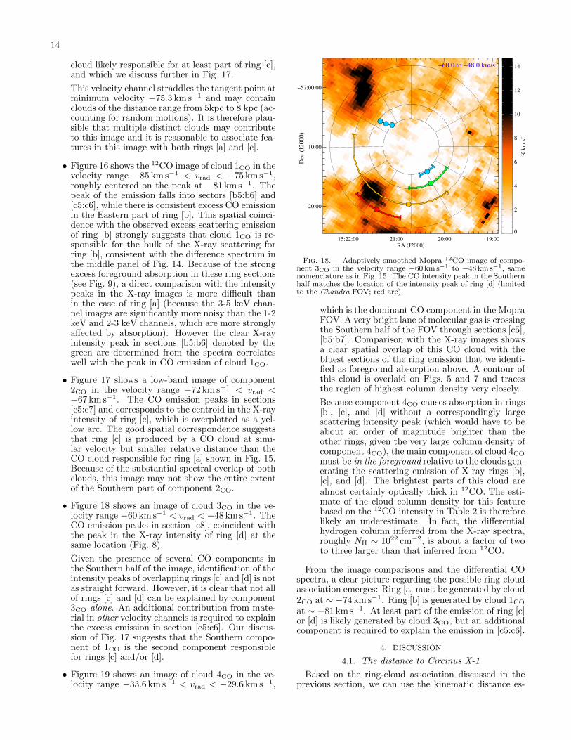
• Figure 16 shows the 12CO image of cloud 1CO in thevelocity range −85 km s−1 < vrad < −75 km s−1,roughly centered on the peak at −81 km s−1. Thepeak of the emission falls into sectors [b5:b6] and[c5:c6], while there is consistent excess CO emissionin the Eastern part of ring [b]. This spatial coinci-dence with the observed excess scattering emissionof ring [b] strongly suggests that cloud 1CO is re-sponsible for the bulk of the X-ray scattering forring [b], consistent with the difference spectrum inthe middle panel of Fig. 14. Because of the strongexcess foreground absorption in these ring sections(see Fig. 9), a direct comparison with the intensitypeaks in the X-ray images is more difficult thanin the case of ring [a] (because the 3-5 keV chan-nel images are significantly more noisy than the 1-2keV and 2-3 keV channels, which are more stronglyaffected by absorption). However the clear X-rayintensity peak in sections [b5:b6] denoted by thegreen arc determined from the spectra correlateswell with the peak in CO emission of cloud 1CO.
• Figure 17 shows a low-band image of component2CO in the velocity range −72 km s−1 < vrad <−67 km s−1. The CO emission peaks in sections[c5:c7] and corresponds to the centroid in the X-rayintensity of ring [c], which is overplotted as a yel-low arc. The good spatial correspondence suggeststhat ring [c] is produced by a CO cloud at simi-lar velocity but smaller relative distance than theCO cloud responsible for ring [a] shown in Fig. 15.Because of the substantial spectral overlap of bothclouds, this image may not show the entire extentof the Southern part of component 2CO.
• Figure 18 shows an image of cloud 3CO in the ve-locity range −60 km s−1 < vrad < −48 km s−1. TheCO emission peaks in section [c8], coincident withthe peak in the X-ray intensity of ring [d] at thesame location (Fig. 8).
Given the presence of several CO components inthe Southern half of the image, identification of theintensity peaks of overlapping rings [c] and [d] is notas straight forward. However, it is clear that not allof rings [c] and [d] can be explained by component3CO alone. An additional contribution from mate-rial in other velocity channels is required to explainthe excess emission in section [c5:c6]. Our discus-sion of Fig. 17 suggests that the Southern compo-nent of 1CO is the second component responsiblefor rings [c] and/or [d].
• Figure 19 shows an image of cloud 4CO in the ve-locity range −33.6 km s−1 < vrad < −29.6 km s−1,
0
2
4
6
8
10
12
14
K k
m s
−1
15:22:00 21:00 20:00 19:00
RA (J2000)
20:00
10:00
−57:00:00
Dec (
J2000)
−60.0 to −48.0 km/s
Fig. 18.— Adaptively smoothed Mopra 12CO image of compo-nent 3CO in the velocity range −60 km s−1 to −48 km s−1, samenomenclature as in Fig. 15. The CO intensity peak in the Southernhalf matches the location of the intensity peak of ring [d] (limitedto the Chandra FOV; red arc).
which is the dominant CO component in the MopraFOV. A very bright lane of molecular gas is crossingthe Southern half of the FOV through sections [c5],[b5:b7]. Comparison with the X-ray images showsa clear spatial overlap of this CO cloud with thebluest sections of the ring emission that we identi-fied as foreground absorption above. A contour ofthis cloud is overlaid on Figs. 5 and 7 and tracesthe region of highest column density very closely.
Because component 4CO causes absorption in rings[b], [c], and [d] without a correspondingly largescattering intensity peak (which would have to beabout an order of magnitude brighter than theother rings, given the very large column density ofcomponent 4CO), the main component of cloud 4CO
must be in the foreground relative to the clouds gen-erating the scattering emission of X-ray rings [b],[c], and [d]. The brightest parts of this cloud arealmost certainly optically thick in 12CO. The esti-mate of the cloud column density for this featurebased on the 12CO intensity in Table 2 is thereforelikely an underestimate. In fact, the differentialhydrogen column inferred from the X-ray spectra,roughly NH ∼ 1022 cm−2, is about a factor of twoto three larger than that inferred from 12CO.
From the image comparisons and the differential COspectra, a clear picture regarding the possible ring-cloudassociation emerges: Ring [a] must be generated by cloud2CO at ∼ −74 km s−1. Ring [b] is generated by cloud 1CO
at ∼ −81 km s−1. At least part of the emission of ring [c]or [d] is likely generated by cloud 3CO, but an additionalcomponent is required to explain the emission in [c5:c6].
4. DISCUSSION
4.1. The distance to Circinus X-1
Based on the ring-cloud association discussed in theprevious section, we can use the kinematic distance es-
15
0
10
20
30
40
K k
m s
−1
15:22:00 21:00 20:00 19:00
RA (J2000)
20:00
10:00
−57:00:00
Dec (
J2000)
−33.6 to −29.6 km/s
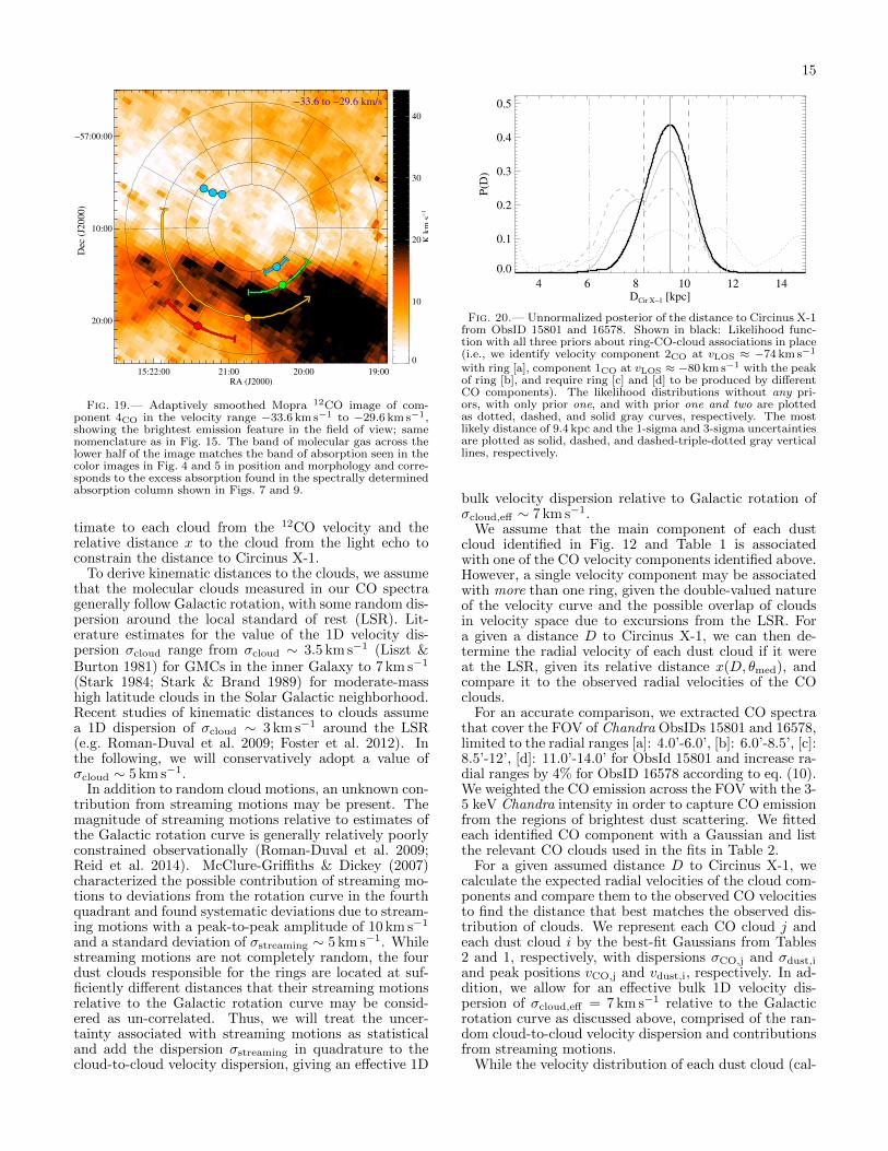
Fig. 19.— Adaptively smoothed Mopra 12CO image of com-ponent 4CO in the velocity range −33.6 km s−1 to −29.6 km s−1,showing the brightest emission feature in the field of view; samenomenclature as in Fig. 15. The band of molecular gas across thelower half of the image matches the band of absorption seen in thecolor images in Fig. 4 and 5 in position and morphology and corre-sponds to the excess absorption found in the spectrally determinedabsorption column shown in Figs. 7 and 9.
timate to each cloud from the 12CO velocity and therelative distance x to the cloud from the light echo toconstrain the distance to Circinus X-1.
To derive kinematic distances to the clouds, we assumethat the molecular clouds measured in our CO spectragenerally follow Galactic rotation, with some random dis-persion around the local standard of rest (LSR). Lit-erature estimates for the value of the 1D velocity dis-persion σcloud range from σcloud ∼ 3.5 km s−1 (Liszt &Burton 1981) for GMCs in the inner Galaxy to 7 km s−1
(Stark 1984; Stark & Brand 1989) for moderate-masshigh latitude clouds in the Solar Galactic neighborhood.Recent studies of kinematic distances to clouds assumea 1D dispersion of σcloud ∼ 3 km s−1 around the LSR(e.g. Roman-Duval et al. 2009; Foster et al. 2012). Inthe following, we will conservatively adopt a value ofσcloud ∼ 5 km s−1.
In addition to random cloud motions, an unknown con-tribution from streaming motions may be present. Themagnitude of streaming motions relative to estimates ofthe Galactic rotation curve is generally relatively poorlyconstrained observationally (Roman-Duval et al. 2009;Reid et al. 2014). McClure-Griffiths & Dickey (2007)characterized the possible contribution of streaming mo-tions to deviations from the rotation curve in the fourthquadrant and found systematic deviations due to stream-ing motions with a peak-to-peak amplitude of 10 km s−1
and a standard deviation of σstreaming ∼ 5 km s−1. Whilestreaming motions are not completely random, the fourdust clouds responsible for the rings are located at suf-ficiently different distances that their streaming motionsrelative to the Galactic rotation curve may be consid-ered as un-correlated. Thus, we will treat the uncer-tainty associated with streaming motions as statisticaland add the dispersion σstreaming in quadrature to thecloud-to-cloud velocity dispersion, giving an effective 1D
4 6 8 10 12 14DCir X−1 [kpc]
0.0
0.1
0.2
0.3
0.4
0.5
P(D
)
Fig. 20.— Unnormalized posterior of the distance to Circinus X-1from ObsID 15801 and 16578. Shown in black: Likelihood func-tion with all three priors about ring-CO-cloud associations in place(i.e., we identify velocity component 2CO at vLOS ≈ −74 km s−1
with ring [a], component 1CO at vLOS ≈ −80 km s−1 with the peakof ring [b], and require ring [c] and [d] to be produced by differentCO components). The likelihood distributions without any pri-ors, with only prior one, and with prior one and two are plottedas dotted, dashed, and solid gray curves, respectively. The mostlikely distance of 9.4 kpc and the 1-sigma and 3-sigma uncertaintiesare plotted as solid, dashed, and dashed-triple-dotted gray verticallines, respectively.
bulk velocity dispersion relative to Galactic rotation ofσcloud,eff ∼ 7 km s−1.
We assume that the main component of each dustcloud identified in Fig. 12 and Table 1 is associatedwith one of the CO velocity components identified above.However, a single velocity component may be associatedwith more than one ring, given the double-valued natureof the velocity curve and the possible overlap of cloudsin velocity space due to excursions from the LSR. Fora given a distance D to Circinus X-1, we can then de-termine the radial velocity of each dust cloud if it wereat the LSR, given its relative distance x(D, θmed), andcompare it to the observed radial velocities of the COclouds.
For an accurate comparison, we extracted CO spectrathat cover the FOV of Chandra ObsIDs 15801 and 16578,limited to the radial ranges [a]: 4.0’-6.0’, [b]: 6.0’-8.5’, [c]:8.5’-12’, [d]: 11.0’-14.0’ for ObsId 15801 and increase ra-dial ranges by 4% for ObsID 16578 according to eq. (10).We weighted the CO emission across the FOV with the 3-5 keV Chandra intensity in order to capture CO emissionfrom the regions of brightest dust scattering. We fittedeach identified CO component with a Gaussian and listthe relevant CO clouds used in the fits in Table 2.
For a given assumed distance D to Circinus X-1, wecalculate the expected radial velocities of the cloud com-ponents and compare them to the observed CO velocitiesto find the distance that best matches the observed dis-tribution of clouds. We represent each CO cloud j andeach dust cloud i by the best-fit Gaussians from Tables2 and 1, respectively, with dispersions σCO,j and σdust,i
and peak positions vCO,j and vdust,i, respectively. In ad-dition, we allow for an effective bulk 1D velocity dis-persion of σcloud,eff = 7 km s−1 relative to the Galacticrotation curve as discussed above, comprised of the ran-dom cloud-to-cloud velocity dispersion and contributionsfrom streaming motions.
While the velocity distribution of each dust cloud (cal-
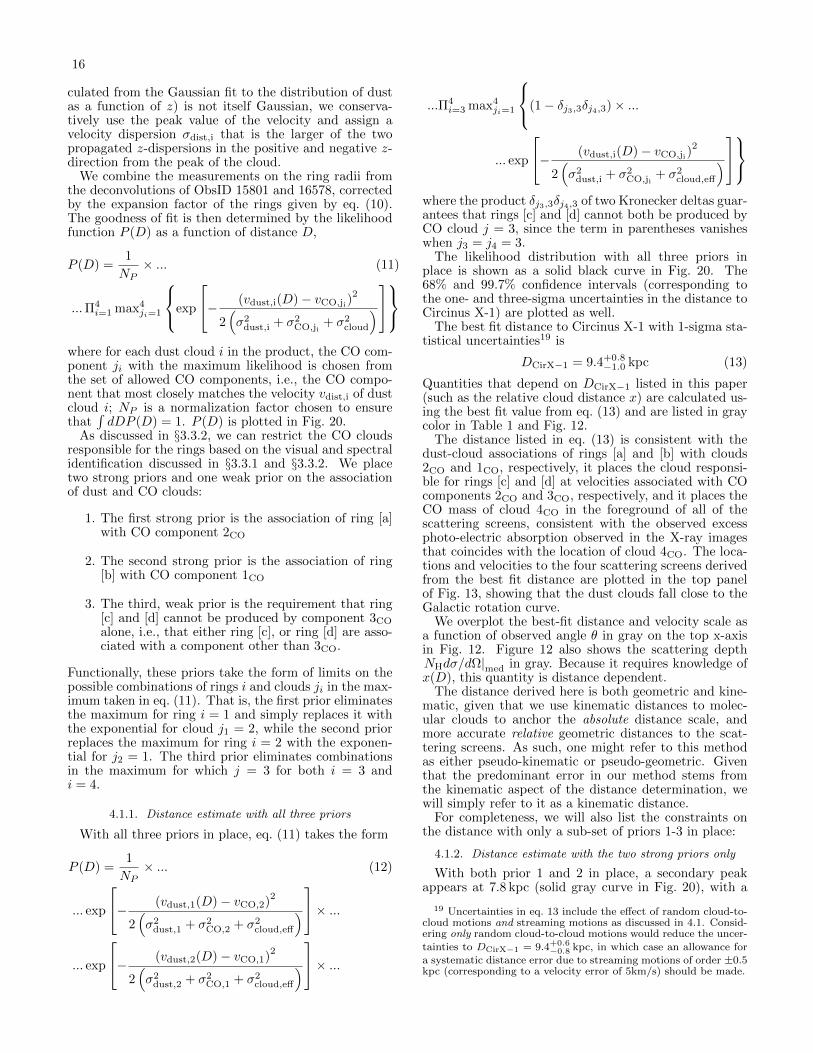
16
culated from the Gaussian fit to the distribution of dustas a function of z) is not itself Gaussian, we conserva-tively use the peak value of the velocity and assign avelocity dispersion σdist,i that is the larger of the twopropagated z-dispersions in the positive and negative z-direction from the peak of the cloud.
We combine the measurements on the ring radii fromthe deconvolutions of ObsID 15801 and 16578, correctedby the expansion factor of the rings given by eq. (10).The goodness of fit is then determined by the likelihoodfunction P (D) as a function of distance D,
P (D) =1
NP× ... (11)
...Π4i=1 max4
ji=1
exp
− (vdust,i(D)− vCO,ji)2
2(σ2
dust,i + σ2CO,ji
+ σ2cloud
)
where for each dust cloud i in the product, the CO com-ponent ji with the maximum likelihood is chosen fromthe set of allowed CO components, i.e., the CO compo-nent that most closely matches the velocity vdist,i of dustcloud i; NP is a normalization factor chosen to ensurethat
∫dDP (D) = 1. P (D) is plotted in Fig. 20.
As discussed in §3.3.2, we can restrict the CO cloudsresponsible for the rings based on the visual and spectralidentification discussed in §3.3.1 and §3.3.2. We placetwo strong priors and one weak prior on the associationof dust and CO clouds:
1. The first strong prior is the association of ring [a]with CO component 2CO
2. The second strong prior is the association of ring[b] with CO component 1CO
3. The third, weak prior is the requirement that ring[c] and [d] cannot be produced by component 3CO
alone, i.e., that either ring [c], or ring [d] are asso-ciated with a component other than 3CO.
Functionally, these priors take the form of limits on thepossible combinations of rings i and clouds ji in the max-imum taken in eq. (11). That is, the first prior eliminatesthe maximum for ring i = 1 and simply replaces it withthe exponential for cloud j1 = 2, while the second priorreplaces the maximum for ring i = 2 with the exponen-tial for j2 = 1. The third prior eliminates combinationsin the maximum for which j = 3 for both i = 3 andi = 4.
4.1.1. Distance estimate with all three priors
With all three priors in place, eq. (11) takes the form
P (D) =1
NP× ... (12)
... exp
− (vdust,1(D)− vCO,2)2
2(σ2
dust,1 + σ2CO,2 + σ2
cloud,eff
)× ...
... exp
− (vdust,2(D)− vCO,1)2
2(σ2
dust,2 + σ2CO,1 + σ2
cloud,eff
)× ...
...Π4i=3 max4
ji=1
(1− δj3,3δj4,3)× ...
... exp
− (vdust,i(D)− vCO,ji)2
2(σ2
dust,i + σ2CO,ji
+ σ2cloud,eff
)
where the product δj3,3δj4,3 of two Kronecker deltas guar-antees that rings [c] and [d] cannot both be produced byCO cloud j = 3, since the term in parentheses vanisheswhen j3 = j4 = 3.
The likelihood distribution with all three priors inplace is shown as a solid black curve in Fig. 20. The68% and 99.7% confidence intervals (corresponding tothe one- and three-sigma uncertainties in the distance toCircinus X-1) are plotted as well.
The best fit distance to Circinus X-1 with 1-sigma sta-tistical uncertainties19 is
DCirX−1 = 9.4+0.8−1.0 kpc (13)
Quantities that depend on DCirX−1 listed in this paper(such as the relative cloud distance x) are calculated us-ing the best fit value from eq. (13) and are listed in graycolor in Table 1 and Fig. 12.
The distance listed in eq. (13) is consistent with thedust-cloud associations of rings [a] and [b] with clouds2CO and 1CO, respectively, it places the cloud responsi-ble for rings [c] and [d] at velocities associated with COcomponents 2CO and 3CO, respectively, and it places theCO mass of cloud 4CO in the foreground of all of thescattering screens, consistent with the observed excessphoto-electric absorption observed in the X-ray imagesthat coincides with the location of cloud 4CO. The loca-tions and velocities to the four scattering screens derivedfrom the best fit distance are plotted in the top panelof Fig. 13, showing that the dust clouds fall close to theGalactic rotation curve.
We overplot the best-fit distance and velocity scale asa function of observed angle θ in gray on the top x-axisin Fig. 12. Figure 12 also shows the scattering depthNHdσ/dΩ|med in gray. Because it requires knowledge ofx(D), this quantity is distance dependent.
The distance derived here is both geometric and kine-matic, given that we use kinematic distances to molec-ular clouds to anchor the absolute distance scale, andmore accurate relative geometric distances to the scat-tering screens. As such, one might refer to this methodas either pseudo-kinematic or pseudo-geometric. Giventhat the predominant error in our method stems fromthe kinematic aspect of the distance determination, wewill simply refer to it as a kinematic distance.
For completeness, we will also list the constraints onthe distance with only a sub-set of priors 1-3 in place:
4.1.2. Distance estimate with the two strong priors only
With both prior 1 and 2 in place, a secondary peakappears at 7.8 kpc (solid gray curve in Fig. 20), with a
19 Uncertainties in eq. 13 include the effect of random cloud-to-cloud motions and streaming motions as discussed in 4.1. Consid-ering only random cloud-to-cloud motions would reduce the uncer-
tainties to DCirX−1 = 9.4+0.6−0.8 kpc, in which case an allowance for
a systematic distance error due to streaming motions of order ±0.5kpc (corresponding to a velocity error of 5km/s) should be made.
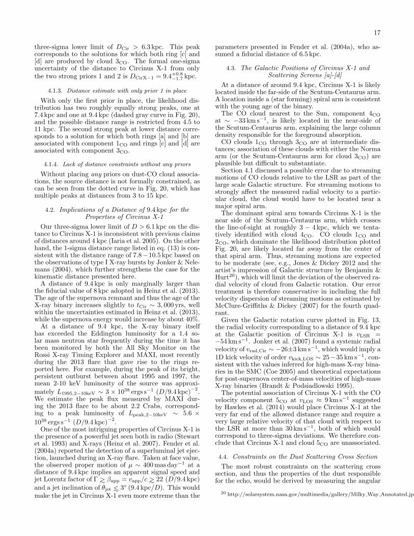
17
three-sigma lower limit of DCir > 6.3 kpc. This peakcorresponds to the solutions for which both ring [c] and[d] are produced by cloud 3CO. The formal one-sigmauncertainty of the distance to Circinus X-1 from onlythe two strong priors 1 and 2 is DCirX−1 = 9.4+0.8
−1.7 kpc.
4.1.3. Distance estimate with only prior 1 in place
With only the first prior in place, the likelihood dis-tribution has two roughly equally strong peaks, one at7.4 kpc and one at 9.4 kpc (dashed gray curve in Fig. 20),and the possible distance range is restricted from 4.5 to11 kpc. The second strong peak at lower distance corre-sponds to a solution for which both rings [a] and [b] areassociated with component 1CO and rings [c] and [d] areassociated with component 3CO.
4.1.4. Lack of distance constraints without any priors
Without placing any priors on dust-CO cloud associa-tions, the source distance is not formally constrained, ascan be seen from the dotted curve in Fig. 20, which hasmultiple peaks at distances from 3 to 15 kpc.
4.2. Implications of a Distance of 9.4 kpc for theProperties of Circinus X-1
Our three-sigma lower limit of D > 6.1 kpc on the dis-tance to Circinus X-1 is inconsistent with previous claimsof distances around 4 kpc (Iaria et al. 2005). On the otherhand, the 1-sigma distance range listed in eq. (13) is con-sistent with the distance range of 7.8−10.5 kpc based onthe observations of type I X-ray bursts by Jonker & Nele-mans (2004), which further strengthens the case for thekinematic distance presented here.
A distance of 9.4 kpc is only marginally larger thanthe fiducial value of 8 kpc adopted in Heinz et al. (2013).The age of the supernova remnant and thus the age of theX-ray binary increases slightly to tCir ∼ 3, 000 yrs, wellwithin the uncertainties estimated in Heinz et al. (2013),while the supernova energy would increase by about 40%.
At a distance of 9.4 kpc, the X-ray binary itselfhas exceeded the Eddington luminosity for a 1.4 so-lar mass neutron star frequently during the time it hasbeen monitored by both the All Sky Monitor on theRossi X-ray Timing Explorer and MAXI, most recentlyduring the 2013 flare that gave rise to the rings re-ported here. For example, during the peak of its bright,persistent outburst between about 1995 and 1997, themean 2-10 keV luminosity of the source was approxi-mately L1995,2−10keV ∼ 3 × 1038 ergs s−1 (D/9.4 kpc)
−2.
We estimate the peak flux measured by MAXI dur-ing the 2013 flare to be about 2.2 Crabs, correspond-ing to a peak luminosity of Lpeak,2−10keV ∼ 5.6 ×1038 ergs s−1 (D/9.4 kpc)
−2.
One of the most intriguing properties of Circinus X-1 isthe presence of a powerful jet seen both in radio (Stewartet al. 1993) and X-rays (Heinz et al. 2007). Fender et al.(2004a) reported the detection of a superluminal jet ejec-tion, launched during an X-ray flare. Taken at face value,the observed proper motion of µ ∼ 400 mas day−1 at adistance of 9.4 kpc implies an apparent signal speed andjet Lorentz factor of Γ ∼> βapp = vapp/c ∼> 22 (D/9.4 kpc)
and a jet inclination of θjet ∼< 3 (9.4 kpc/D). This wouldmake the jet in Circinus X-1 even more extreme than the
parameters presented in Fender et al. (2004a), who as-sumed a fiducial distance of 6.5 kpc.
4.3. The Galactic Positions of Circinus X-1 andScattering Screens [a]-[d]
At a distance of around 9.4 kpc, Circinus X-1 is likelylocated inside the far-side of the Scutum-Centaurus arm.A location inside a (star forming) spiral arm is consistentwith the young age of the binary.
The CO cloud nearest to the Sun, component 4CO
at ∼ −33 km s−1, is likely located in the near-side ofthe Scutum-Centaurus arm, explaining the large columndensity responsible for the foreground absorption.
CO clouds 1CO through 3CO are at intermediate dis-tances; association of these clouds with either the Normaarm (or the Scutum-Centaurus arm for cloud 3CO) areplausible but difficult to substantiate.
Section 4.1 discussed a possible error due to streamingmotions of CO clouds relative to the LSR as part of thelarge scale Galactic structure. For streaming motions tostrongly affect the measured radial velocity to a partic-ular cloud, the cloud would have to be located near amajor spiral arm.
The dominant spiral arm towards Circinus X-1 is thenear side of the Scutum-Centaurus arm, which crossesthe line-of-sight at roughly 3 − 4 kpc, which we tenta-tively identified with cloud 4CO. CO clouds 1CO and2CO, which dominate the likelihood distribution plottedFig. 20, are likely located far away from the center ofthat spiral arm. Thus, streaming motions are expectedto be moderate (see, e.g., Jones & Dickey 2012 and theartist’s impression of Galactic structure by Benjamin &Hurt20), which will limit the deviation of the observed ra-dial velocity of cloud from Galactic rotation. Our errortreatment is therefore conservative in including the fullvelocity dispersion of streaming motions as estimated byMcClure-Griffiths & Dickey (2007) for the fourth quad-rant.
Given the Galactic rotation curve plotted in Fig. 13,the radial velocity corresponding to a distance of 9.4 kpcat the Galactic position of Circinus X-1 is vLSR =−54 km s−1. Jonker et al. (2007) found a systemic radialvelocity of vrad,Cir ∼ −26±3 km s−1, which would imply a1D kick velocity of order vkick,LOS ∼ 25−35 km s−1, con-sistent with the values inferred for high-mass X-ray bina-ries in the SMC (Coe 2005) and theoretical expectationsfor post-supernova center-of-mass velocities of high-massX-ray binaries (Brandt & Podsiadlowski 1995).
The potential association of Circinus X-1 with the COvelocity component 5CO at vLOS ≈ 9 km s−1 suggestedby Hawkes et al. (2014) would place Circinus X-1 at thevery far end of the allowed distance range and require avery large relative velocity of that cloud with respect tothe LSR at more than 30 km s−1, both of which wouldcorrespond to three-sigma deviations. We therefore con-clude that Circinus X-1 and cloud 5CO are unassociated.
4.4. Constraints on the Dust Scattering Cross Section
The most robust constraints on the scattering crosssection, and thus the properties of the dust responsiblefor the echo, would be derived by measuring the angular
20 http://solarsystem.nasa.gov/multimedia/gallery/Milky Way Annotated.jpg
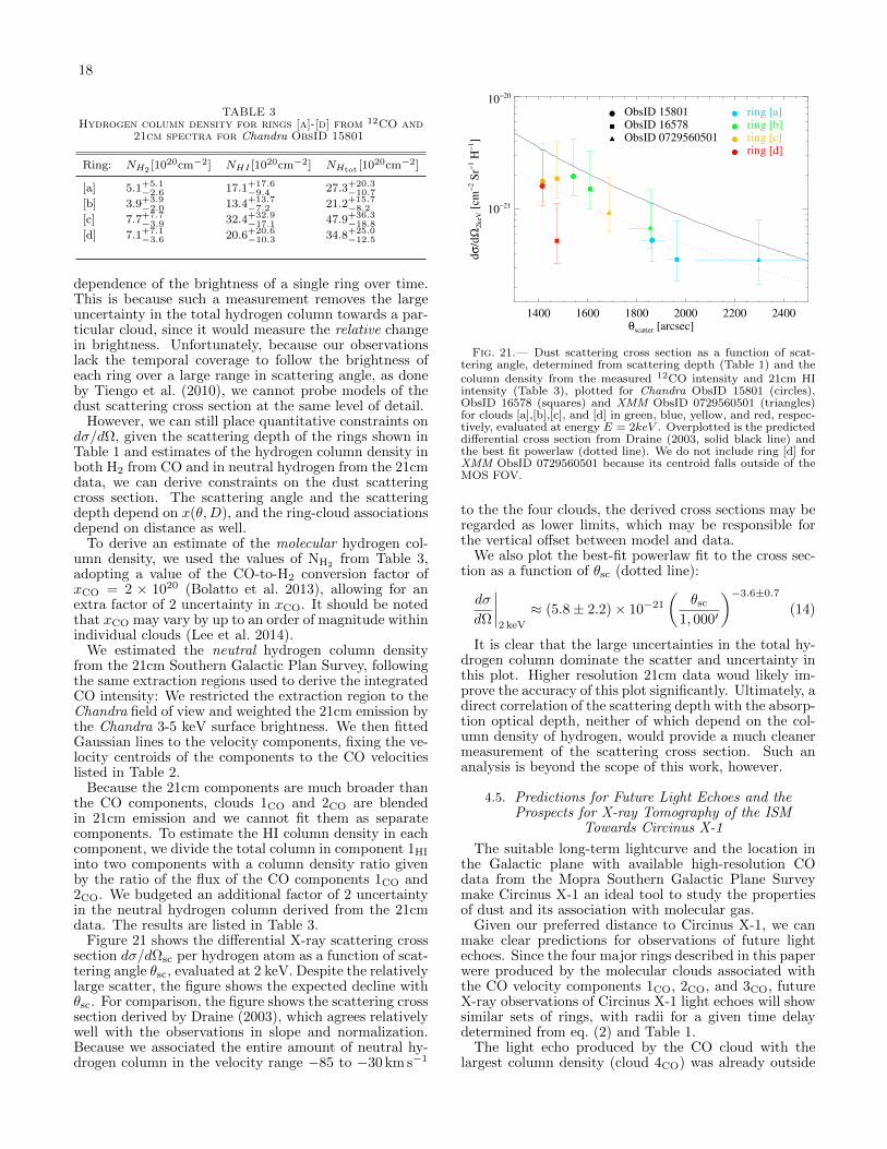
18
TABLE 3Hydrogen column density for rings [a]-[d] from 12CO and
21cm spectra for Chandra ObsID 15801
Ring: NH2 [1020cm−2] NHI [1020cm−2] NHtot [1020cm−2]
[a] 5.1+5.1−2.6 17.1+17.6
−9.4 27.3+20.3−10.7
[b] 3.9+3.9−2.0 13.4+13.7
−7.2 21.2+15.7−8.2
[c] 7.7+7.7−3.9 32.4+32.9
−17.1 47.9+36.3−18.8
[d] 7.1+7.1−3.6 20.6+20.6
−10.3 34.8+25.0−12.5
dependence of the brightness of a single ring over time.This is because such a measurement removes the largeuncertainty in the total hydrogen column towards a par-ticular cloud, since it would measure the relative changein brightness. Unfortunately, because our observationslack the temporal coverage to follow the brightness ofeach ring over a large range in scattering angle, as doneby Tiengo et al. (2010), we cannot probe models of thedust scattering cross section at the same level of detail.
However, we can still place quantitative constraints ondσ/dΩ, given the scattering depth of the rings shown inTable 1 and estimates of the hydrogen column density inboth H2 from CO and in neutral hydrogen from the 21cmdata, we can derive constraints on the dust scatteringcross section. The scattering angle and the scatteringdepth depend on x(θ,D), and the ring-cloud associationsdepend on distance as well.
To derive an estimate of the molecular hydrogen col-umn density, we used the values of NH2 from Table 3,adopting a value of the CO-to-H2 conversion factor ofxCO = 2 × 10²⁰ (Bolatto et al. 2013), allowing for anextra factor of 2 uncertainty in xCO. It should be notedthat xCO may vary by up to an order of magnitude withinindividual clouds (Lee et al. 2014).
We estimated the neutral hydrogen column densityfrom the 21cm Southern Galactic Plan Survey, followingthe same extraction regions used to derive the integratedCO intensity: We restricted the extraction region to theChandra field of view and weighted the 21cm emission bythe Chandra 3-5 keV surface brightness. We then fittedGaussian lines to the velocity components, fixing the ve-locity centroids of the components to the CO velocitieslisted in Table 2.
Because the 21cm components are much broader thanthe CO components, clouds 1CO and 2CO are blendedin 21cm emission and we cannot fit them as separatecomponents. To estimate the HI column density in eachcomponent, we divide the total column in component 1HI
into two components with a column density ratio givenby the ratio of the flux of the CO components 1CO and2CO. We budgeted an additional factor of 2 uncertaintyin the neutral hydrogen column derived from the 21cmdata. The results are listed in Table 3.
Figure 21 shows the differential X-ray scattering crosssection dσ/dΩsc per hydrogen atom as a function of scat-tering angle θsc, evaluated at 2 keV. Despite the relativelylarge scatter, the figure shows the expected decline withθsc. For comparison, the figure shows the scattering crosssection derived by Draine (2003), which agrees relativelywell with the observations in slope and normalization.Because we associated the entire amount of neutral hy-drogen column in the velocity range −85 to −30 km s−1
1400 1600 1800 2000 2200 2400θscatter [arcsec]
10−21
10−20
dσ
/dΩ
2k
eV [
cm−
2 S
r−1 H
−1]
ObsID 15801ObsID 16578ObsID 0729560501
ring [a]ring [b]ring [c]ring [d]
Fig. 21.— Dust scattering cross section as a function of scat-tering angle, determined from scattering depth (Table 1) and thecolumn density from the measured 12CO intensity and 21cm HIintensity (Table 3), plotted for Chandra ObsID 15801 (circles),ObsID 16578 (squares) and XMM ObsID 0729560501 (triangles)for clouds [a],[b],[c], and [d] in green, blue, yellow, and red, respec-tively, evaluated at energy E = 2keV . Overplotted is the predicteddifferential cross section from Draine (2003, solid black line) andthe best fit powerlaw (dotted line). We do not include ring [d] forXMM ObsID 0729560501 because its centroid falls outside of theMOS FOV.
to the the four clouds, the derived cross sections may beregarded as lower limits, which may be responsible forthe vertical offset between model and data.
We also plot the best-fit powerlaw fit to the cross sec-tion as a function of θsc (dotted line):
dσ
dΩ
∣∣∣∣2 keV
≈ (5.8± 2.2)× 10−21
(θsc
1, 000′
)−3.6±0.7
(14)
It is clear that the large uncertainties in the total hy-drogen column dominate the scatter and uncertainty inthis plot. Higher resolution 21cm data woud likely im-prove the accuracy of this plot significantly. Ultimately, adirect correlation of the scattering depth with the absorp-tion optical depth, neither of which depend on the col-umn density of hydrogen, would provide a much cleanermeasurement of the scattering cross section. Such ananalysis is beyond the scope of this work, however.
4.5. Predictions for Future Light Echoes and theProspects for X-ray Tomography of the ISM
Towards Circinus X-1
The suitable long-term lightcurve and the location inthe Galactic plane with available high-resolution COdata from the Mopra Southern Galactic Plane Surveymake Circinus X-1 an ideal tool to study the propertiesof dust and its association with molecular gas.
Given our preferred distance to Circinus X-1, we canmake clear predictions for observations of future lightechoes. Since the four major rings described in this paperwere produced by the molecular clouds associated withthe CO velocity components 1CO, 2CO, and 3CO, futureX-ray observations of Circinus X-1 light echoes will showsimilar sets of rings, with radii for a given time delaydetermined from eq. (2) and Table 1.
The light echo produced by the CO cloud with thelargest column density (cloud 4CO) was already outside
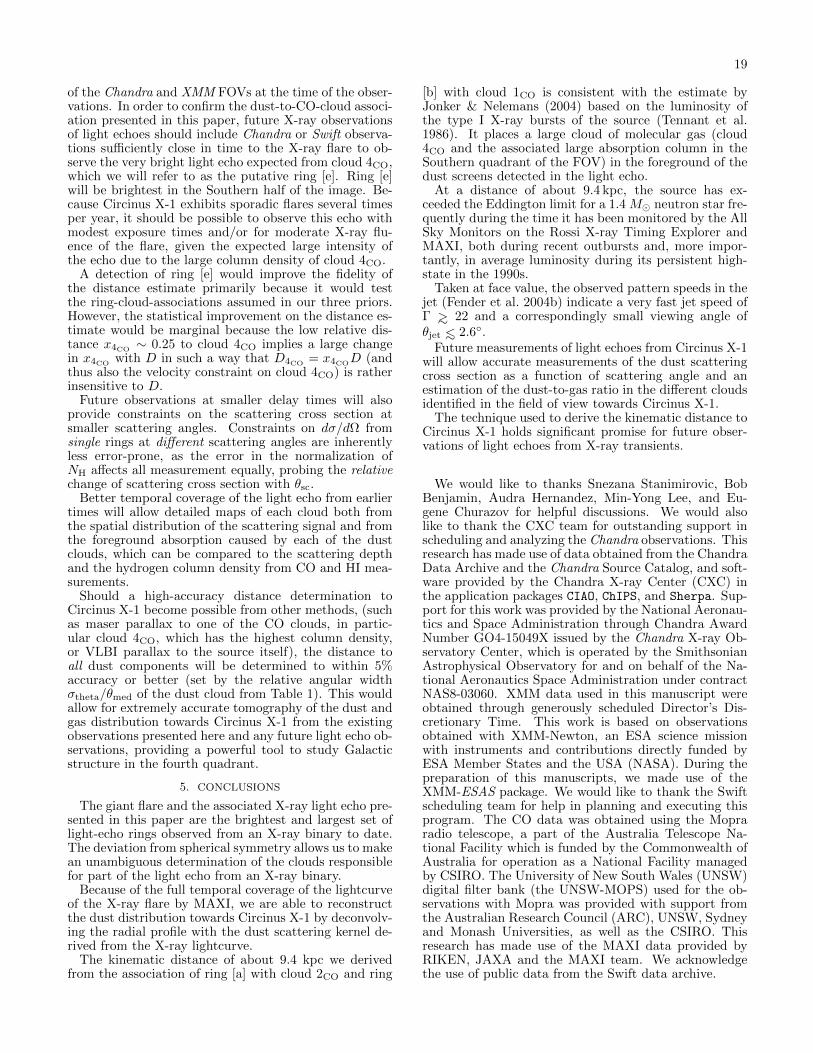
19
of the Chandra and XMM FOVs at the time of the obser-vations. In order to confirm the dust-to-CO-cloud associ-ation presented in this paper, future X-ray observationsof light echoes should include Chandra or Swift observa-tions sufficiently close in time to the X-ray flare to ob-serve the very bright light echo expected from cloud 4CO,which we will refer to as the putative ring [e]. Ring [e]will be brightest in the Southern half of the image. Be-cause Circinus X-1 exhibits sporadic flares several timesper year, it should be possible to observe this echo withmodest exposure times and/or for moderate X-ray flu-ence of the flare, given the expected large intensity ofthe echo due to the large column density of cloud 4CO.
A detection of ring [e] would improve the fidelity ofthe distance estimate primarily because it would testthe ring-cloud-associations assumed in our three priors.However, the statistical improvement on the distance es-timate would be marginal because the low relative dis-tance x4CO
∼ 0.25 to cloud 4CO implies a large changein x4CO with D in such a way that D4CO = x4COD (andthus also the velocity constraint on cloud 4CO) is ratherinsensitive to D.
Future observations at smaller delay times will alsoprovide constraints on the scattering cross section atsmaller scattering angles. Constraints on dσ/dΩ fromsingle rings at different scattering angles are inherentlyless error-prone, as the error in the normalization ofNH affects all measurement equally, probing the relativechange of scattering cross section with θsc.
Better temporal coverage of the light echo from earliertimes will allow detailed maps of each cloud both fromthe spatial distribution of the scattering signal and fromthe foreground absorption caused by each of the dustclouds, which can be compared to the scattering depthand the hydrogen column density from CO and HI mea-surements.
Should a high-accuracy distance determination toCircinus X-1 become possible from other methods, (suchas maser parallax to one of the CO clouds, in partic-ular cloud 4CO, which has the highest column density,or VLBI parallax to the source itself), the distance toall dust components will be determined to within 5%accuracy or better (set by the relative angular widthσtheta/θmed of the dust cloud from Table 1). This wouldallow for extremely accurate tomography of the dust andgas distribution towards Circinus X-1 from the existingobservations presented here and any future light echo ob-servations, providing a powerful tool to study Galacticstructure in the fourth quadrant.
5. CONCLUSIONS
The giant flare and the associated X-ray light echo pre-sented in this paper are the brightest and largest set oflight-echo rings observed from an X-ray binary to date.The deviation from spherical symmetry allows us to makean unambiguous determination of the clouds responsiblefor part of the light echo from an X-ray binary.
Because of the full temporal coverage of the lightcurveof the X-ray flare by MAXI, we are able to reconstructthe dust distribution towards Circinus X-1 by deconvolv-ing the radial profile with the dust scattering kernel de-rived from the X-ray lightcurve.
The kinematic distance of about 9.4 kpc we derivedfrom the association of ring [a] with cloud 2CO and ring
[b] with cloud 1CO is consistent with the estimate byJonker & Nelemans (2004) based on the luminosity ofthe type I X-ray bursts of the source (Tennant et al.1986). It places a large cloud of molecular gas (cloud4CO and the associated large absorption column in theSouthern quadrant of the FOV) in the foreground of thedust screens detected in the light echo.
At a distance of about 9.4 kpc, the source has ex-ceeded the Eddington limit for a 1.4 M neutron star fre-quently during the time it has been monitored by the AllSky Monitors on the Rossi X-ray Timing Explorer andMAXI, both during recent outbursts and, more impor-tantly, in average luminosity during its persistent high-state in the 1990s.
Taken at face value, the observed pattern speeds in thejet (Fender et al. 2004b) indicate a very fast jet speed ofΓ ∼> 22 and a correspondingly small viewing angle ofθjet ∼< 2.6.
Future measurements of light echoes from Circinus X-1will allow accurate measurements of the dust scatteringcross section as a function of scattering angle and anestimation of the dust-to-gas ratio in the different cloudsidentified in the field of view towards Circinus X-1.
The technique used to derive the kinematic distance toCircinus X-1 holds significant promise for future obser-vations of light echoes from X-ray transients.
We would like to thanks Snezana Stanimirovic, BobBenjamin, Audra Hernandez, Min-Yong Lee, and Eu-gene Churazov for helpful discussions. We would alsolike to thank the CXC team for outstanding support inscheduling and analyzing the Chandra observations. Thisresearch has made use of data obtained from the ChandraData Archive and the Chandra Source Catalog, and soft-ware provided by the Chandra X-ray Center (CXC) inthe application packages CIAO, ChIPS, and Sherpa. Sup-port for this work was provided by the National Aeronau-tics and Space Administration through Chandra AwardNumber GO4-15049X issued by the Chandra X-ray Ob-servatory Center, which is operated by the SmithsonianAstrophysical Observatory for and on behalf of the Na-tional Aeronautics Space Administration under contractNAS8-03060. XMM data used in this manuscript wereobtained through generously scheduled Director’s Dis-cretionary Time. This work is based on observationsobtained with XMM-Newton, an ESA science missionwith instruments and contributions directly funded byESA Member States and the USA (NASA). During thepreparation of this manuscripts, we made use of theXMM-ESAS package. We would like to thank the Swiftscheduling team for help in planning and executing thisprogram. The CO data was obtained using the Mopraradio telescope, a part of the Australia Telescope Na-tional Facility which is funded by the Commonwealth ofAustralia for operation as a National Facility managedby CSIRO. The University of New South Wales (UNSW)digital filter bank (the UNSW-MOPS) used for the ob-servations with Mopra was provided with support fromthe Australian Research Council (ARC), UNSW, Sydneyand Monash Universities, as well as the CSIRO. Thisresearch has made use of the MAXI data provided byRIKEN, JAXA and the MAXI team. We acknowledgethe use of public data from the Swift data archive.
20
REFERENCES
Asai, K., Mihara, T., Matsuoka, M., Sugizaki, M., Nakahira, S.,Negoro, H., Nakajima, M., & Okazaki, A. T. 2014, PASJ, 66, 79
Bolatto, A. D., Wolfire, M., & Leroy, A. K. 2013, ARA&A, 51,207
Brand, J. & Blitz, L. 1993, A&A, 275, 67Brandt, N. & Podsiadlowski, P. 1995, MNRAS, 274, 461Brandt, W. N. & Schulz, N. S. 2000, ApJ, 544, L123Burton, M. G., Braiding, C., Glueck, C., Goldsmith, P., Hawkes,
J., Hollenbach, D. J., Kulesa, C., Martin, C. L., Pineda, J. L.,Rowell, G., Simon, R., Stark, A. A., Stutzki, J., Tothill,N. J. H., Urquhart, J. S., Walker, C., Walsh, A. J., & Wolfire,M. 2013, Pub.Astr.Soc.Austr., 30, 44
Calvelo, D. E., Fender, R. P., Tzioumis, A. K., Kawai, N.,Broderick, J. W., & Bell, M. E. 2012, MNRAS, 419, 436
Clarkson, W. I., Charles, P. A., & Onyett, N. 2004, MNRAS, 348,458
Coe, M. J. 2005, MNRAS, 358, 1379Corrales, L. & Paerels, F. 2013, ArXiv e-printsDraine, B. T. 2003, ApJ, 598, 1026Fender, R., Wu, K., Johnston, H., Tzioumis, T., Jonker, P.,
Spencer, R., & van der Klis, M. 2004a, Nature, 427, 222Fender, R. P., Belloni, T. M., & Gallo, E. 2004b, MNRAS, 355,
1105Foster, J. B., Stead, J. J., Benjamin, R. A., Hoare, M. G., &
Jackson, J. M. 2012, ApJ, 751, 157Freeman, P. E., Kashyap, V., Rosner, R., & Lamb, D. Q. 2002,
ApJS, 138, 185Hawkes, J., Rowell, G., Dawson, B., Aharonian, F., Burton, M.,
Fukui, Y., Furukawa, N., Hayakawa, T., Kawamura, A.,Maxted, N., de Ona-Wilhelmi, E., de Wilt, P., & Walsh, A.2014, International Journal of Modern Physics ConferenceSeries, 28, 60198
Heinz, S., Schulz, N. S., Brandt, W. N., & Galloway, D. K. 2007,ApJ, 663, L93
Heinz, S., Sell, P., Fender, R. P., Jonker, P. G., Brandt, W. N.,Calvelo-Santos, D. E., Tzioumis, A. K., Nowak, M. A., Schulz,N. S., Wijnands, R., & van der Klis, M. 2013, ApJ, 779, 171
Hickox, R. C. & Markevitch, M. 2006, ApJ, 645, 95Iaria, R., Spano, M., Di Salvo, T., Robba, N. R., Burderi, L.,
Fender, R., van der Klis, M., & Frontera, F. 2005, ApJ, 619, 503Jones, C. & Dickey, J. M. 2012, ApJ, 753, 62Jonker, P. G. & Nelemans, G. 2004, MNRAS, 354, 355Jonker, P. G., Nelemans, G., & Bassa, C. G. 2007, MNRAS, 374,
999Lee, M.-Y., Stanimirovic, S., Wolfire, M. G., Shetty, R., Glover,
S. C. O., Molina, F. Z., & Klessen, R. S. 2014, ApJ, 784, 80Linares, M., Watts, A., Altamirano, D., Soleri, P., Degenaar, N.,
Yang, Y., Wijnands, R., Casella, P., Homan, J., Chakrabarty,D., Rea, N., Armas-Padilla, M., Cavecchi, Y., Kalamkar, M.,Kaur, R., Patruno, A., & van der Klis, M. 2010, ApJ, 719, L84
Liszt, H. S. & Burton, W. B. 1981, ApJ, 243, 778Lucy, L. B. 1974, AJ, 79, 745Mao, J., Ling, Z., & Zhang, S.-N. 2014, ApJ, 785, 23Mathis, J. S. & Lee, C.-W. 1991, ApJ, 376, 490Matsuoka, M., Kawasaki, K., Ueno, S., Tomida, H., Kohama, M.,
Suzuki, M., Adachi, Y., Ishikawa, M., Mihara, T., Sugizaki, M.,Isobe, N., Nakagawa, Y., Tsunemi, H., Miyata, E., Kawai, N.,Kataoka, J., Morii, M., Yoshida, A., Negoro, H., Nakajima, M.,Ueda, Y., Chujo, H., Yamaoka, K., Yamazaki, O., Nakahira, S.,You, T., Ishiwata, R., Miyoshi, S., Eguchi, S., Hiroi, K.,Katayama, H., & Ebisawa, K. 2009, PASJ, 61, 999
McClure-Griffiths, N. M. & Dickey, J. M. 2007, ApJ, 671, 427McClure-Griffiths, N. M., Dickey, J. M., Gaensler, B. M., Green,
A. J., Haverkorn, M., & Strasser, S. 2005, ApJS, 158, 178McCollough, M. L., Smith, R. K., & Valencic, L. A. 2013, ApJ,
762, 2Nicolson, G. D. 2007, The Astronomer’s Telegram, 985, 1Oosterbroek, T., van der Klis, M., Kuulkers, E., van Paradijs, J.,
& Lewin, W. H. G. 1995, A&A, 297, 141Parkinson, P. M. S., Tournear, D. M., Bloom, E. D., Focke,
W. B., Reilly, K. T., Wood, K. S., Ray, P. S., Wolff, M. T., &Scargle, J. D. 2003, ApJ, 595, 333
Predehl, P. & Schmitt, J. H. M. M. 1995, A&A, 293, 889
Reid, M. J., Menten, K. M., Brunthaler, A., Zheng, X. W., Dame,T. M., Xu, Y., Wu, Y., Zhang, B., Sanna, A., Sato, M.,Hachisuka, K., Choi, Y. K., Immer, K., Moscadelli, L., Rygl,K. L. J., & Bartkiewicz, A. 2014, ApJ, 783, 130
Richardson, W. H. 1972, Journal of the Optical Society ofAmerica (1917-1983), 62, 55
Roman-Duval, J., Jackson, J. M., Heyer, M., Johnson, A.,Rathborne, J., Shah, R., & Simon, R. 2009, ApJ, 699, 1153
Sell, P. H., Heinz, S., Calvelo, D. E., Tudose, V., Soleri, P.,Fender, R. P., Jonker, P. G., Schulz, N. S., Brandt, W. N.,Nowak, M. A., Wijnands, R., van der Klis, M., & Casella, P.2010, ApJ, 719, L194
Seward, F. D. & Smith, R. K. 2013, ApJ, 769, 17Shirey, R. E., Bradt, H. V., Levine, A. M., & Morgan, E. H. 1996,
ApJ, 469, L21Soleri, P., Heinz, S., Fender, R., Wijnands, R., Tudose, V.,
Altamirano, D., Jonker, P. G., van der Klis, M., Kuiper, L.,Kaiser, C., & Casella, P. 2009, MNRAS, 397, L1
Stark, A. A. 1984, ApJ, 281, 624Stark, A. A. & Brand, J. 1989, ApJ, 339, 763Stewart, R. T., Caswell, J. L., Haynes, R. F., & Nelson, G. J.
1993, MNRAS, 261, 593Stewart, R. T., Nelson, G. J., Penninx, W., Kitamoto, S.,
Miyamoto, S., & Nicolson, G. D. 1991, MNRAS, 253, 212Svirski, G., Nakar, E., & Ofek, E. O. 2011, MNRAS, 415, 2485Tennant, A. F., Fabian, A. C., & Shafer, R. A. 1986, MNRAS,
221, 27PTiengo, A., Vianello, G., Esposito, P., Mereghetti, S., Giuliani,
A., Costantini, E., Israel, G. L., Stella, L., Turolla, R., Zane, S.,Rea, N., Gotz, D., Bernardini, F., Moretti, A., Romano, P.,Ehle, M., & Gehrels, N. 2010, ApJ, 710, 227
Tudose, V., Fender, R. P., Kaiser, C. R., Tzioumis, A. K., van derKlis, M., & Spencer, R. E. 2006, MNRAS, 372, 417
Vianello, G., Tiengo, A., & Mereghetti, S. 2007, A&A, 473, 423Xiang, J., Lee, J. C., Nowak, M. A., & Wilms, J. 2011, ApJ, 738,
78