lost relatives of the gumbel trick - matej...

Lost Relatives of the Gumbel Trick

Matej Balog 1 2 Nilesh Tripuraneni 3 Zoubin Ghahramani 1 4 Adrian Weller 1 5

AbstractThe Gumbel trick is a method to sample from adiscrete probability distribution, or to estimate itsnormalizing partition function. The method re-lies on repeatedly applying a random perturba-tion to the distribution in a particular way, eachtime solving for the most likely configuration.We derive an entire family of related methods,of which the Gumbel trick is one member, andshow that the new methods have superior prop-erties in several settings with minimal additionalcomputational cost. In particular, for the Gum-bel trick to yield computational benefits for dis-crete graphical models, Gumbel perturbations onall configurations are typically replaced with so-called low-rank perturbations. We show how asubfamily of our new methods adapts to this set-ting, proving new upper and lower bounds on thelog partition function and deriving a family of se-quential samplers for the Gibbs distribution. Fi-nally, we balance the discussion by showing howthe simpler analytical form of the Gumbel trickenables additional theoretical results.

1. IntroductionIn this work we are concerned with the fundamental prob-lem of sampling from a discrete probability distribution andevaluating its normalizing constant. A probability distribu-tion p on a discrete sample space X is provided in termsof its potential function φ : X → [−∞,∞), correspond-ing to log-unnormalized probabilities via p(x) = eφ(x)/Z,where the normalizing constant Z is the partition function.In this context, p is the Gibbs distribution on X associatedwith the potential function φ. The challenges of samplingfrom such a discrete probability distribution and estimatingthe partition function are fundamental problems with ubiq-

1University of Cambridge, UK 2MPI-IS, Tubingen, Germany3UC Berkeley, USA 4Uber AI Labs, USA 5Alan Turing Institute,UK. Correspondence to: Matej Balog <[email protected]>.Code: https://github.com/matejbalog/gumbel-relatives.

Proceedings of the 34 th International Conference on MachineLearning, Sydney, Australia, PMLR 70, 2017. Copyright 2017by the author(s).

uitous applications in machine learning, classical statisticsand statistical physics (see, e.g., Lauritzen, 1996).

Perturb-and-MAP methods (Papandreou & Yuille, 2010)constitute a class of randomized algorithms for estimatingpartition functions and sampling from Gibbs distributions,which operate by randomly perturbing the correspondingpotential functions and employing maximum a posteriori(MAP) solvers on the perturbed models to find a maximumprobability configuration. This MAP problem is NP-hardin general; however, substantial research effort has led tothe development of solvers which can efficiently computeor estimate the MAP solution on many problems that occurin practice (e.g., Boykov et al., 2001; Kolmogorov, 2006;Darbon, 2009). Evaluating the partition function is a harderproblem, containing for instance #P-hard counting prob-lems. The general aim of perturb-and-MAP methods isto reduce the problem of partition function evaluation, orthe problem of sampling from the Gibbs distribution, to re-peated instances of the MAP problem (where each instanceis on a different random perturbation of the original model).

The Gumbel trick (Papandreou & Yuille, 2011) relies onadding Gumbel-distributed noise to each configuration’spotential φ(x). We derive a wider family of perturb-and-MAP methods that can be seen as perturbing the model indifferent ways – in particular using the Weibull and Frechetdistributions alongside the Gumbel. We show that the newmethods can be implemented with essentially no additionalcomputational cost by simply averaging existing GumbelMAP perturbations in different spaces, and that they canlead to more accurate estimators of the partition function.

Evaluating or perturbing each configuration’s potentialwith i.i.d. Gumbel noise can be computationally expensive.One way to mitigate this is to cleverly prune computationin regions where the maximum perturbed potential is un-likely to be found (Maddison et al., 2014; Chen & Ghahra-mani, 2016). Another approach exploits the product struc-ture of the sample space in discrete graphical models, re-placing i.i.d. Gumbel noise with a “low-rank” approxima-tion. Hazan & Jaakkola (2012); Hazan et al. (2013) showedthat from such an approximation, upper and lower boundson the partition function and a sequential sampler for theGibbs distribution can still be recovered. We show that asubfamily of our new methods, consisting of Frechet, Ex-ponential and Weibull tricks, can also be used with low-

https://github.com/matejbalog/gumbel-relatives


rank perturbations, and use these tricks to derive new upperand lower bounds on the partition function, and to constructnew sequential samplers for the Gibbs distribution.

Our main contributions are as follows:

1. A family of tricks that can be implemented by simplyaveraging Gumbel perturbations in different spaces, andwhich can lead to more accurate or more sample effi-cient estimators of Z (Section 2).

2. New upper and lower bounds on the partition function ofa discrete graphical model computable using low-rankperturbations, and a corresponding family of sequentialsamplers for the Gibbs distribution (Section 3).

3. Discussion of advantages of the simpler analytical formof the Gumbel trick including new links between the er-rors of estimating Z, sampling, and entropy estimationusing low-rank Gumbel perturbations (Section 4).

Background and Related work The idea of perturbingthe potential function of a discrete graphical model in or-der to sample from its associated Gibbs distribution was in-troduced by Papandreou & Yuille (2011), inspired by theirprevious work on reducing the sampling problem for Gaus-sian Markov random fields to the problem of finding themean, using independent local perturbations of each Gaus-sian factor (Papandreou & Yuille, 2010). Tarlow et al.(2012) extended this perturb-and-MAP approach to sam-pling, in particular by considering more general structuredprediction problems. Hazan & Jaakkola (2012) pointed outthat MAP perturbations are useful not only for sampling theGibbs distribution (considering the argmax of the perturbedmodel), but also for bounding and approximating the parti-tion function (by considering the value of the max).

Afterwards, Hazan et al. (2013) derived new lower boundson the partition function and proposed a new sampler forthe Gibbs distribution that samples variables of a discretegraphical model sequentially, using expected values of low-rank MAP perturbations to construct the conditional proba-bilities. Due to the low-rank approximation, this algorithmhas the option to reject a sample. Orabona et al. (2014)and Hazan et al. (2016) subsequently derived measure con-centration results for the Gumbel distribution that can beused to control the rejection probability. Maji et al. (2014)derived an uncertainty measure from random MAP pertur-bations, using it within a Bayesian active learning frame-work for interactive image boundary annotation.

Perturb-and-MAP was famously generalized to continuousspaces by Maddison et al. (2014), replacing the Gumbeldistribution with a Gumbel process and calling the resultingalgorithm A* sampling. Maddison (2016) cast this workinto a unified framework together with adaptive rejectionsampling techniques, based on the notion of exponentialraces. This recent view generally brings together perturb-

and-MAP and accept-reject samplers, exploiting the con-nection between the Gumbel distribution and competingexponential clocks that we also discuss in Section 2.1.

Inspired by A* sampling, Kim et al. (2016) proposed an ex-act sampler for discrete graphical models based on lazily-instantiated random perturbations, which uses linear pro-gramming relaxations to prune the optimization space. Fur-ther recent applications of perturb-and-MAP include struc-tured prediction in computer vision (Bertasius et al., 2017)and turning the discrete sampling problem into an opti-mization task that can be cast as a multi-armed bandit prob-lem (Chen & Ghahramani, 2016), see Section 5.2 below.

In addition to perturb-and-MAP methods, we are aware ofthree other approaches to estimate the partition functionof a discrete graphical model via MAP solver calls. TheWISH method (weighted-integrals-and-sums-by-hashing,Ermon et al., 2013) relies on repeated MAP inference callsapplied to the model after subjecting it to random hash con-straints. The Frank-Wolfe method may be applied by itera-tively updating marginals using a constrained MAP solverand line search (Belanger et al., 2013; Krishnan et al.,2015). Weller & Jebara (2014a) instead use just one MAPcall over a discretized mesh of marginals to approximatethe Bethe partition function, which itself is an estimate(which often performs well) of the true partition function.

2. Relatives of the Gumbel TrickIn this section, we review the Gumbel trick and state themechanism by which it can be generalized into an entirefamily of tricks. We show how these tricks can equivalentlybe viewed as averaging standard Gumbel perturbations indifferent spaces, instantiate several examples, and comparethe various tricks’ properties.

Notation Throughout this paper, let X be a finite samplespace of size N := |X |. Let p : X → [0,∞) be an unnor-malized mass function over X and let Z :=

∑x∈X p(x) be

its normalizing partition function. Write p(x) := p(x)/Zfor the normalized version of p, and φ(x) := ln p(x) for thelog-unnormalized probabilities, i.e. the potential function.

We write Exp(λ) for the exponential distribution with rate(inverse mean) λ and Gumbel(µ) for the Gumbel distribu-tion with location µ and scale 1. The latter has mean µ+ c,where c ≈ 0.5772 is the Euler-Mascheroni constant.

2.1. The Gumbel Trick

Similarly to the connection between the Gumbel trick andthe Poisson process established by Maddison (2016), weintroduce the Gumbel trick for discrete probability distri-butions using a simple and elegant construction via com-peting exponential clocks. ConsiderN independent clocks,


Table 1: New tricks for constructing unbiased estimators of different transformations f(Z) of the partition function.

Trick g(x) Mean f(Z) Variance of g(T ) Asymptotic var. of Z

Gumbel − lnx− c lnZ π2

6π2

6Z2

Exponential x 1Z

1Z2 Z2

Weibull α xα, α > 0 Z−αΓ(1 + α) Γ(1+2α)−Γ(1+α)2

Z2α1α2

(Γ(1+2α)

Γ(1+α)2− 1

)Z2

Frechet α xα, α ∈ (−1, 0) Z−αΓ(1 + α) Γ(1+2α)−Γ(1+α)2

Z2α for α > − 12

1α2

(Γ(1+2α)

Γ(1+α)2− 1

)Z2

Pareto ex ZZ−1

for Z > 1 a Z(Z−1)2(Z−2)

for Z > 2 Z2

(Z−2)2

Tail t 1{x>t} e−tZ e−tZ(1− e−tZ) (1−e−tZ)2

t2

started simultaneously, such that the j-th clock rings aftera random time Tj ∼ Exp(λj). Then it is easy to show that(1) the time until some clock rings has Exp(

∑Nj=1 λj) dis-

tribution, and (2) the probability of the j-th clock ringingfirst is proportional to its rate λj . These properties are alsowidely used in survival analysis (Cox & Oakes, 1984).

Consider N competing exponential clocks {Tx}x∈X , in-dexed by elements of X , with respective rates λx = p(x).Property (1) of competing exponential clocks tells us that

minx∈X{Tx} ∼ Exp(Z). (1)

Property (2) says that the random variable argminx Tx, tak-ing values in X , is distributed according to p:

argminx∈X

{Tx} ∼ p. (2)

The Gumbel trick is obtained by applying the functiong(x) = − lnx − c to the equalities in distribution (1)and (2). When g is applied to an Exp(λ) random vari-able, the result follows the Gumbel(−c + lnλ) distribu-tion, which can also be represented as lnλ + γ, whereγ ∼ Gumbel(−c). Defining {γ(x)}x∈X

i.i.d.∼ Gumbel(−c)and noting that g is strictly decreasing, applying the func-tion g to equalities in distribution (1) and (2), we obtain:

maxx∈X{φ(x) + γ(x)} ∼ Gumbel(−c+ lnZ), (1’)

argmaxx∈X

{φ(x) + γ(x)} ∼ p, (2’)

where we have recalled that φ(x) = lnλx = ln p(x). Thedistribution Gumbel(−c + lnZ) has mean lnZ, and thusthe log partition function can be estimated by averagingsamples (Hazan & Jaakkola, 2012).

2.2. Constructing New Tricks

Given the equality in distribution (1), we can treat the prob-lem of estimating the partition function Z as a parameterestimation problem for the exponential distribution. Ap-plying the function g(x) = − lnx − c as in the Gumbeltrick to obtain a Gumbel(−c+ lnZ) random variable, and

estimating its mean to obtain an unbiased estimator of lnZ,is just one way of inferring information about Z.

We consider applying different functions g to (1); par-ticularly those functions g that transform the exponentialdistribution to another distribution with known mean. Asthe original exponential distribution has rate Z, the trans-formed distribution will have mean f(Z), where f will ingeneral no longer be the logarithm function. Since we oftenare interested in estimating various transformations f(Z)of Z, this provides us a with a collection of unbiased es-timators from which to choose. Moreover, further trans-forming these estimators yields a collection of (biased) es-timators for other transformations of Z, including Z itself.Example 1 (Weibull tricks). For any α > 0, applyingthe function g(x) = xα to an Exp(λ) random variableyields a random variable with the Weibull(λ−α, α−1) dis-tribution with scale λ−α and shape α−1, which has meanλ−αΓ(1 + α) and can be also represented as λ−αW ,where W ∼ Weibull(1, α−1). Defining {W (x)}x∈X

i.i.d.∼Weibull(1, α−1) and noting that g is increasing, applyingg to the equality in distribution (1) gives

minx∈X{p−αW (x)} ∼Weibull(Z−α, α−1). (1”)

Estimating the mean of Weibull(Z−α, α−1) yields an un-biased estimator of Z−αΓ(1 + α). The special case α = 1corresponds to the identity function g(x) = x; we call theresulting trick the Exponential trick.

Table 1 lists several examples of tricks derived this way.As Example 1 shows, these tricks may not involve addi-tive perturbation of the potential function φ(x); the Weibulltricks multiplicatively perturb exponentiated unnormalizedprobabilities p−α with Weibull noise. As models of inter-est are often specified in terms of potential functions, to beable to reuse existing MAP solvers in a black-box mannerwith the new tricks, we seek an equivalent formulation interms of the potential function. The following Propositionshows that by not passing the function g through the mini-mization in equation (1), the new tricks can be equivalentlyformulated as averaging additive Gumbel perturbations ofthe potential function in different spaces.


101 102 103 104

number of samples M

10-4

10-3

10-2

10-1

100

101

MSE o

f Z

, in

unit

s of Z

2

Gumbel: MSE

Gumbel: var

Exponential: MSE

Exponential: var

100 101 102 103 104

number of samples M

10-4

10-3

10-2

10-1

100

101

MSE o

f lnZ

, in

unit

s of

1

Gumbel: MSE

Exponential: MSE

Exponential: var

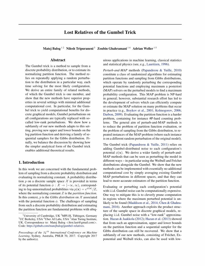
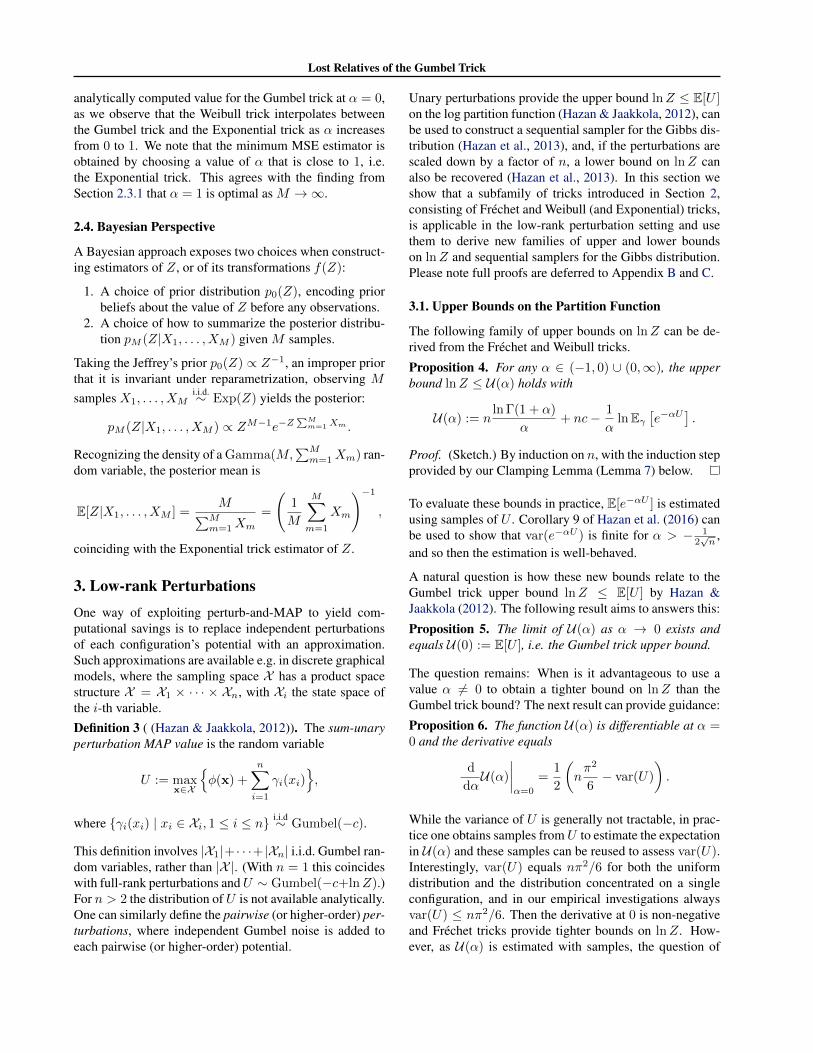
Figure 1: Analytically computed MSE and variance of Gumbeland Exponential trick estimators of Z (left) and lnZ (right). TheMSEs are dominated by the variance, so the dashed and solid linesmostly overlap. See Section 2.3.2 for details.

Proposition 2. For any function g : [0,∞)→ R such thatf(Z) = ET∼Exp(Z)[g(T )] exists, we have

f(Z) = Eγ[g

(e−c exp

(−maxx∈X{φ(x) + γ(x)}

))],

where {γ(x)}x∈Xi.i.d.∼ Gumbel(−c).

Proof. As maxx{φ(x) + γ(x)} ∼ Gumbel(−c + lnZ),we have e−c exp(maxx{φ(x) +γ(x)}) ∼ Exp(Z) and theresult follows by the assumption relating f and g.

Proposition 2 shows that the new tricks can be implementedby solving the same MAP problems maxx{φ(x)+γ(x)} asin the Gumbel trick, and then merely passing the solutionsthrough the function x 7→ g(e−c exp(x)) before averagingthem to approximate the expectation.

2.3. Comparing Tricks

2.3.1. ASYMPTOTIC EFFICIENCY

The Delta method (Casella & Berger, 2002) is a simpletechnique for assessing the asymptotic variance of esti-mators that are obtained by a differentiable transforma-tion of an estimator with known variance. The last col-umn in Table 1 lists asymptotic variances of correspond-ing tricks when unbiased estimators of f(Z) are passedthrough the function f−1 to yield (biased, but consistentand non-negative) estimators of Z itself. It is interestingto examine the constants that multiply Z2 in some of theobtained asymptotic variance expressions for the differenttricks. For example, it can be shown using Gurland’s ra-tio (Gurland, 1956) that this constant is at least 1 for theWeibull and Frechet tricks, which is precisely the valueachieved by the Exponential trick (which corresponds toα = 1). Moreover, the Gumbel trick constant π2/6 can beshown to be the limit as α → 0 of the Weibull and Frechettrick constants. In particular, the constant of the Exponen-tial trick is strictly better than that of the standard Gumbeltrick: 1 < π2/6 ≈ 1.65. This motivates us to compare theGumbel and Exponential tricks in more detail.

0.0 0.5 1.0 1.5 2.0α

10-2

10-1

100

101

MSE o

f est

imato

rs o

f Z

, in

unit

s of Z

2

M= 4

M= 8

M= 16

M= 32

M= 64

M= 128

Gumbel trick(α= 0, theoretical)

Exponential trick(α= 1, theoretical)

0.0 0.5 1.0 1.5 2.0α

10-2

10-1

100

101

MSE o

f est

imato

rs o

f lnZ

, in

unit

s of

1

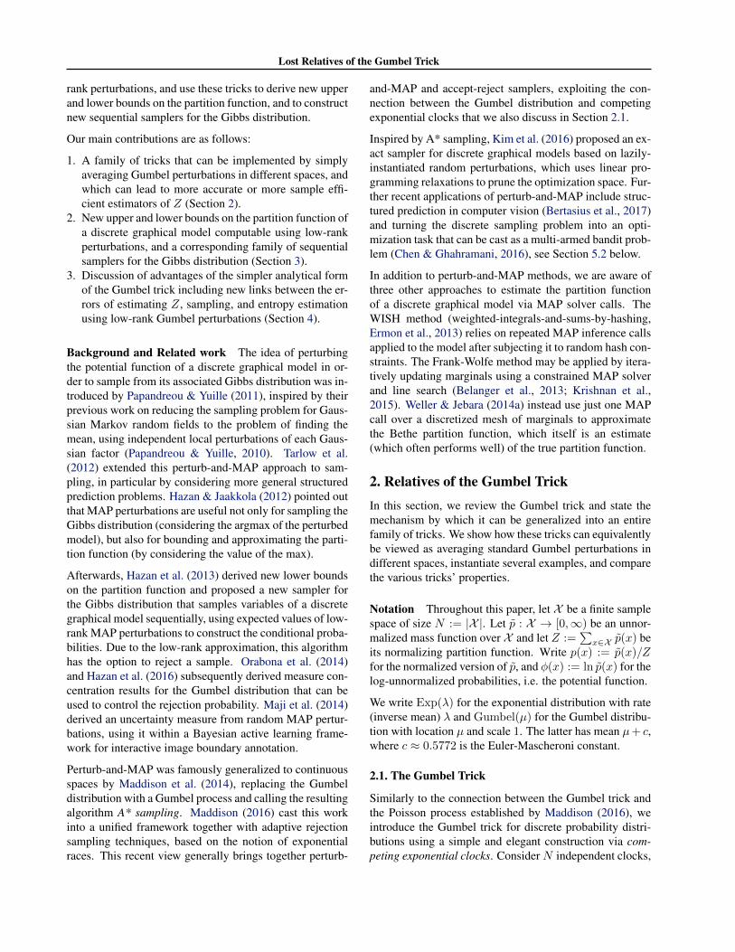
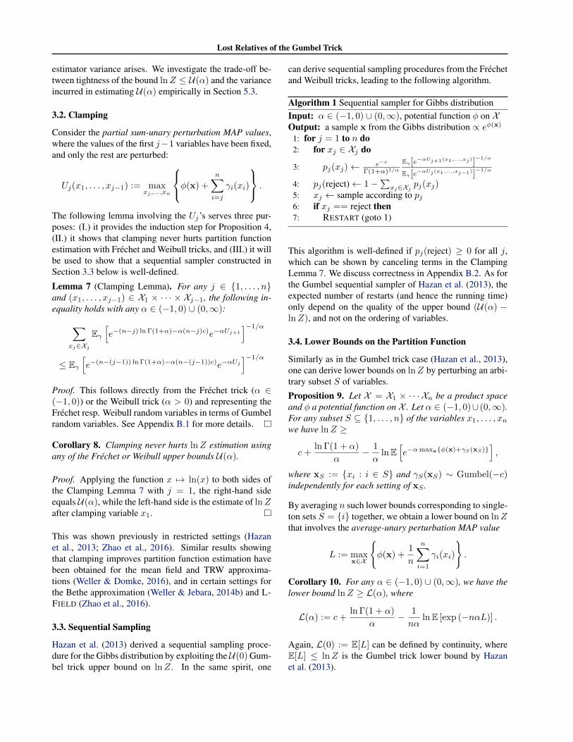
Figure 2: MSE of estimators of Z (left) and lnZ (right) stem-ming from Frechet (− 1

2< α < 0), Gumbel (α = 0) and Weibull

tricks (α > 0). See Section 2.3.2 for details.

2.3.2. MEAN SQUARED ERROR (MSE)

For estimators Y , their MSE(Y ) = var(Y ) + bias(Y )2 isa commonly used comparison metric. When the Gumbel orExponential tricks are used to estimate either Z or lnZ, thebiases, variances, and MSEs of the estimators can be com-puted analytically using standard methods (Appendix A).

For example, the unbiased estimator of lnZ from the Gum-bel trick can be turned into a consistent non-negative esti-mator of Z by exponentiation: Y = exp( 1

M

∑Mm=1Xm),

where X1, . . . , XMi.i.d.∼ Gumbel(−c + lnZ) are obtained

using equation (1’). The bias and variance of Y can becomputed using independence and the moment generatingfunctions of the Xm’s, see Appendix A for details.

Perhaps surprisingly, all estimator properties only dependon the true value of Z and not on the structure of the model(distribution p), since the estimators rely only on i.i.d. sam-ples of a Gumbel(−c + lnZ) random variable. Figure 1shows the analytically computed estimator variances andMSEs. For estimating Z itself (left), the Exponential trickoutperforms the Gumbel trick in terms of MSE for all sam-ple sizes M ≥ 3 (for M ∈ {1, 2}, both estimators haveinfinite variance and MSE). The ratio of MSEs quickly ap-proaches π2/6, and in this regime the Exponential trick re-quires 1 − 6/π2 ≈ 39% fewer samples than the Gumbeltrick to reach the same MSE. Also, for estimating lnZ,(Figure 1, right), the Exponential trick provides a lowerMSE estimator for sample sizes M ≥ 2; only for M = 1the Gumbel trick provides a better estimator.

Note that as biases are available analytically, the estima-tors can be easily debiased (by subtracting their bias). Onethen obtain estimators with MSEs equal to the variances ofthe original estimators, shown dashed in Figure 1. The Ex-ponential trick would then always outperform the Gumbeltrick when estimating lnZ, even with sample size M = 1.

For Weibull tricks with α 6= 1 and Frechet tricks, we esti-mated the biases and variances of estimators of Z and lnZby constructing K = 100, 000 estimators in each case andevaluating their bias and variance. Figure 2 shows the re-sults for varying α and several sample sizesM . We plot the


analytically computed value for the Gumbel trick at α = 0,as we observe that the Weibull trick interpolates betweenthe Gumbel trick and the Exponential trick as α increasesfrom 0 to 1. We note that the minimum MSE estimator isobtained by choosing a value of α that is close to 1, i.e.the Exponential trick. This agrees with the finding fromSection 2.3.1 that α = 1 is optimal as M →∞.

2.4. Bayesian Perspective

A Bayesian approach exposes two choices when construct-ing estimators of Z, or of its transformations f(Z):

1. A choice of prior distribution p0(Z), encoding priorbeliefs about the value of Z before any observations.

2. A choice of how to summarize the posterior distribu-tion pM (Z|X1, . . . , XM ) given M samples.

Taking the Jeffrey’s prior p0(Z) ∝ Z−1, an improper priorthat it is invariant under reparametrization, observing Msamples X1, . . . , XM

i.i.d.∼ Exp(Z) yields the posterior:

pM (Z|X1, . . . , XM ) ∝ ZM−1e−Z∑Mm=1 Xm .

Recognizing the density of a Gamma(M,∑Mm=1Xm) ran-

dom variable, the posterior mean is

E[Z|X1, . . . , XM ] =M∑M

m=1Xm

=

(1

M

M∑m=1

Xm

)−1

,

coinciding with the Exponential trick estimator of Z.

3. Low-rank PerturbationsOne way of exploiting perturb-and-MAP to yield com-putational savings is to replace independent perturbationsof each configuration’s potential with an approximation.Such approximations are available e.g. in discrete graphicalmodels, where the sampling space X has a product spacestructure X = X1 × · · · × Xn, with Xi the state space ofthe i-th variable.Definition 3 ( (Hazan & Jaakkola, 2012)). The sum-unaryperturbation MAP value is the random variable

U := maxx∈X

{φ(x) +

n∑i=1

γi(xi)},

where {γi(xi) | xi ∈ Xi, 1 ≤ i ≤ n}i.i.d∼ Gumbel(−c).

This definition involves |X1|+ · · ·+ |Xn| i.i.d. Gumbel ran-dom variables, rather than |X |. (With n = 1 this coincideswith full-rank perturbations andU ∼ Gumbel(−c+lnZ).)For n > 2 the distribution of U is not available analytically.One can similarly define the pairwise (or higher-order) per-turbations, where independent Gumbel noise is added toeach pairwise (or higher-order) potential.

Unary perturbations provide the upper bound lnZ ≤ E[U ]on the log partition function (Hazan & Jaakkola, 2012), canbe used to construct a sequential sampler for the Gibbs dis-tribution (Hazan et al., 2013), and, if the perturbations arescaled down by a factor of n, a lower bound on lnZ canalso be recovered (Hazan et al., 2013). In this section weshow that a subfamily of tricks introduced in Section 2,consisting of Frechet and Weibull (and Exponential) tricks,is applicable in the low-rank perturbation setting and usethem to derive new families of upper and lower boundson lnZ and sequential samplers for the Gibbs distribution.Please note full proofs are deferred to Appendix B and C.

3.1. Upper Bounds on the Partition Function

The following family of upper bounds on lnZ can be de-rived from the Frechet and Weibull tricks.

Proposition 4. For any α ∈ (−1, 0) ∪ (0,∞), the upperbound lnZ ≤ U(α) holds with

U(α) := nln Γ(1 + α)

α+ nc− 1

αlnEγ

[e−αU

].

Proof. (Sketch.) By induction on n, with the induction stepprovided by our Clamping Lemma (Lemma 7) below.

To evaluate these bounds in practice, E[e−αU ] is estimatedusing samples of U . Corollary 9 of Hazan et al. (2016) canbe used to show that var(e−αU ) is finite for α > − 1

2√n

,and so then the estimation is well-behaved.

A natural question is how these new bounds relate to theGumbel trick upper bound lnZ ≤ E[U ] by Hazan &Jaakkola (2012). The following result aims to answers this:

Proposition 5. The limit of U(α) as α → 0 exists andequals U(0) := E[U ], i.e. the Gumbel trick upper bound.

The question remains: When is it advantageous to use avalue α 6= 0 to obtain a tighter bound on lnZ than theGumbel trick bound? The next result can provide guidance:

Proposition 6. The function U(α) is differentiable at α =0 and the derivative equals

d

dαU(α)

∣∣∣∣α=0

=1

2

(nπ2

6− var(U)

).

While the variance of U is generally not tractable, in prac-tice one obtains samples fromU to estimate the expectationin U(α) and these samples can be reused to assess var(U).Interestingly, var(U) equals nπ2/6 for both the uniformdistribution and the distribution concentrated on a singleconfiguration, and in our empirical investigations alwaysvar(U) ≤ nπ2/6. Then the derivative at 0 is non-negativeand Frechet tricks provide tighter bounds on lnZ. How-ever, as U(α) is estimated with samples, the question of


estimator variance arises. We investigate the trade-off be-tween tightness of the bound lnZ ≤ U(α) and the varianceincurred in estimating U(α) empirically in Section 5.3.

3.2. Clamping

Consider the partial sum-unary perturbation MAP values,where the values of the first j−1 variables have been fixed,and only the rest are perturbed:

Uj(x1, . . . , xj−1) := maxxj ,...,xn

φ(x) +

n∑i=j

γi(xi)

.

The following lemma involving the Uj’s serves three pur-poses: (I.) it provides the induction step for Proposition 4,(II.) it shows that clamping never hurts partition functionestimation with Frechet and Weibull tricks, and (III.) it willbe used to show that a sequential sampler constructed inSection 3.3 below is well-defined.

Lemma 7 (Clamping Lemma). For any j ∈ {1, . . . , n}and (x1, . . . , xj−1) ∈ X1 × · · · × Xj−1, the following in-equality holds with any α ∈ (−1, 0) ∪ (0,∞):∑

xj∈Xj

Eγ[e−(n−j) ln Γ(1+α)−α(n−j)c)e−αUj+1

]−1/α

≤ Eγ[e−(n−(j−1)) ln Γ(1+α)−α(n−(j−1))c)e−αUj

]−1/α

Proof. This follows directly from the Frechet trick (α ∈(−1, 0)) or the Weibull trick (α > 0) and representing theFrechet resp. Weibull random variables in terms of Gumbelrandom variables. See Appendix B.1 for more details.

Corollary 8. Clamping never hurts lnZ estimation usingany of the Frechet or Weibull upper bounds U(α).

Proof. Applying the function x 7→ ln(x) to both sides ofthe Clamping Lemma 7 with j = 1, the right-hand sideequals U(α), while the left-hand side is the estimate of lnZafter clamping variable x1.

This was shown previously in restricted settings (Hazanet al., 2013; Zhao et al., 2016). Similar results showingthat clamping improves partition function estimation havebeen obtained for the mean field and TRW approxima-tions (Weller & Domke, 2016), and in certain settings forthe Bethe approximation (Weller & Jebara, 2014b) and L-FIELD (Zhao et al., 2016).

3.3. Sequential Sampling

Hazan et al. (2013) derived a sequential sampling proce-dure for the Gibbs distribution by exploiting the U(0) Gum-bel trick upper bound on lnZ. In the same spirit, one

can derive sequential sampling procedures from the Frechetand Weibull tricks, leading to the following algorithm.

Algorithm 1 Sequential sampler for Gibbs distributionInput: α ∈ (−1, 0) ∪ (0,∞), potential function φ on XOutput: a sample x from the Gibbs distribution ∝ eφ(x)

1: for j = 1 to n do2: for xj ∈ Xj do

3: pj(xj)← e−c

Γ(1+α)1/α

Eγ [e−αUj+1(x1,...,xj)]−1/α

Eγ [e−αUj(x1,...,xj−1)]−1/α

4: pj(reject)← 1−∑xj∈Xj pj(xj)

5: xj ← sample according to pj6: if xj == reject then7: RESTART (goto 1)

This algorithm is well-defined if pj(reject) ≥ 0 for all j,which can be shown by canceling terms in the ClampingLemma 7. We discuss correctness in Appendix B.2. As forthe Gumbel sequential sampler of Hazan et al. (2013), theexpected number of restarts (and hence the running time)only depend on the quality of the upper bound (U(α) −lnZ), and not on the ordering of variables.

3.4. Lower Bounds on the Partition Function

Similarly as in the Gumbel trick case (Hazan et al., 2013),one can derive lower bounds on lnZ by perturbing an arbi-trary subset S of variables.

Proposition 9. Let X = X1 × · · · Xn be a product spaceand φ a potential function on X . Let α ∈ (−1, 0)∪ (0,∞).For any subset S ⊆ {1, . . . , n} of the variables x1, . . . , xnwe have lnZ ≥

c+ln Γ(1 + α)

α− 1

αlnE

[e−αmaxx{φ(x)+γS(xS)}

],

where xS := {xi : i ∈ S} and γS(xS) ∼ Gumbel(−c)independently for each setting of xS .

By averaging n such lower bounds corresponding to single-ton sets S = {i} together, we obtain a lower bound on lnZthat involves the average-unary perturbation MAP value

L := maxx∈X

{φ(x) +

1

n

n∑i=1

γi(xi)

}.

Corollary 10. For any α ∈ (−1, 0) ∪ (0,∞), we have thelower bound lnZ ≥ L(α), where

L(α) := c+ln Γ(1 + α)

α− 1

nαlnE [exp (−nαL)] .

Again, L(0) := E[L] can be defined by continuity, whereE[L] ≤ lnZ is the Gumbel trick lower bound by Hazanet al. (2013).


4. Advantages of the Gumbel TrickWe have seen how the Gumbel trick can be embedded intoa continuous family of tricks, consisting of Frechet, Expo-nential, and Weibull tricks. We showed that the new trickscan provide more efficient estimators of the partition func-tion in the full-rank perturbation setting (Section 2), andin the low-rank perturbation setting lead to sequential sam-plers and new bounds on lnZ, which can be also more ef-ficient, as we investigate in Section 5.3. To balance thediscussion of merits of different tricks, in this section webriefly highlight advantages of the Gumbel trick that stemfrom its simpler analytical form.

First, by consulting Table 1 we see that the function g(x) =− lnx−c has the property that the variance of the resultingestimator (of lnZ) does not depend on the value of Z; thefunction g is a variance stabilizing transformation for theExponential distribution.

Second, exploiting the fact that the logarithm function leadsto additive perturbations, Maji et al. (2014) showed that theentropy of x∗, the configuration with maximum potentialafter sum-unary perturbation in the sense of Definition 3,can be bounded as H(x∗) ≤ B(p) :=

∑ni=1 Eγi [γi(x

∗i )].

We extend this result to show how the errors of boundinglnZ, sampling, and entropy estimation are related:Proposition 11. Writing p for the Gibbs distribution andB(p) := Eγi [γi(x

∗i )] for the entropy bound, we have

(U(0)− lnZ)︸︷︷︸error in lnZ bound

+ KL(x∗ ‖ p)︸︷︷︸sampling error

= B(p)−H(x∗)︸︷︷︸error in entropy estimation

.

Third, the additive character of the Gumbel perturbationscan also be used to derive a new result relating the error ofthe lower bound L(0) and of sampling x∗∗ as the configu-ration achieving the maximum average-unary perturbationvalue L, instead of sampling from the Gibbs distribution p:Proposition 12. Writing p for the Gibbs distribution,

lnZ − L(0)︸︷︷︸error in lnZ bound

≥ KL(x∗∗ ‖ p)︸︷︷︸sampling error

≥ 0.

Remark. While we knew from Hazan et al. (2013) thatlnZ − L(0) ≥ 0, this is a stronger result showing thatthe size of the gap is an upper bound on the KL divergencebetween the approximate sampling distribution of x∗∗ andthe Gibbs distribution p.

Proofs of the new results appear in Appendix B.3 and C.2.

Fourth, viewed as a function of the Gumbel perturbationsγ, the random variable U has a bounded gradient, allowingearlier measure concentration results (Orabona et al., 2014;Hazan et al., 2016). Proving similar measure concentrationresults for the expectations E[e−αU ] appearing in U(α) forα 6= 0 may be more challenging.

5. ExperimentsWe conducted experiments with the following aims:

1. To show that the higher efficiency of the Exponentialtrick in the full-rank perturbation setting is useful inpractice, we compared it to the Gumbel trick in A*sampling (Maddison et al., 2014) (Section 5.1) and inthe large-scale discrete sampling setting of Chen &Ghahramani (2016) (Section 5.2).

2. To show that non-zero values of α can lead to bet-ter estimators of lnZ in the low-rank perturbation set-ting as well, we compare the Frechet and Weibull trickbounds U(α) to the Gumbel trick bound U(0) on acommon discrete graphical model with different cou-pling strengths; see Section 5.3.

5.1. A* Sampling

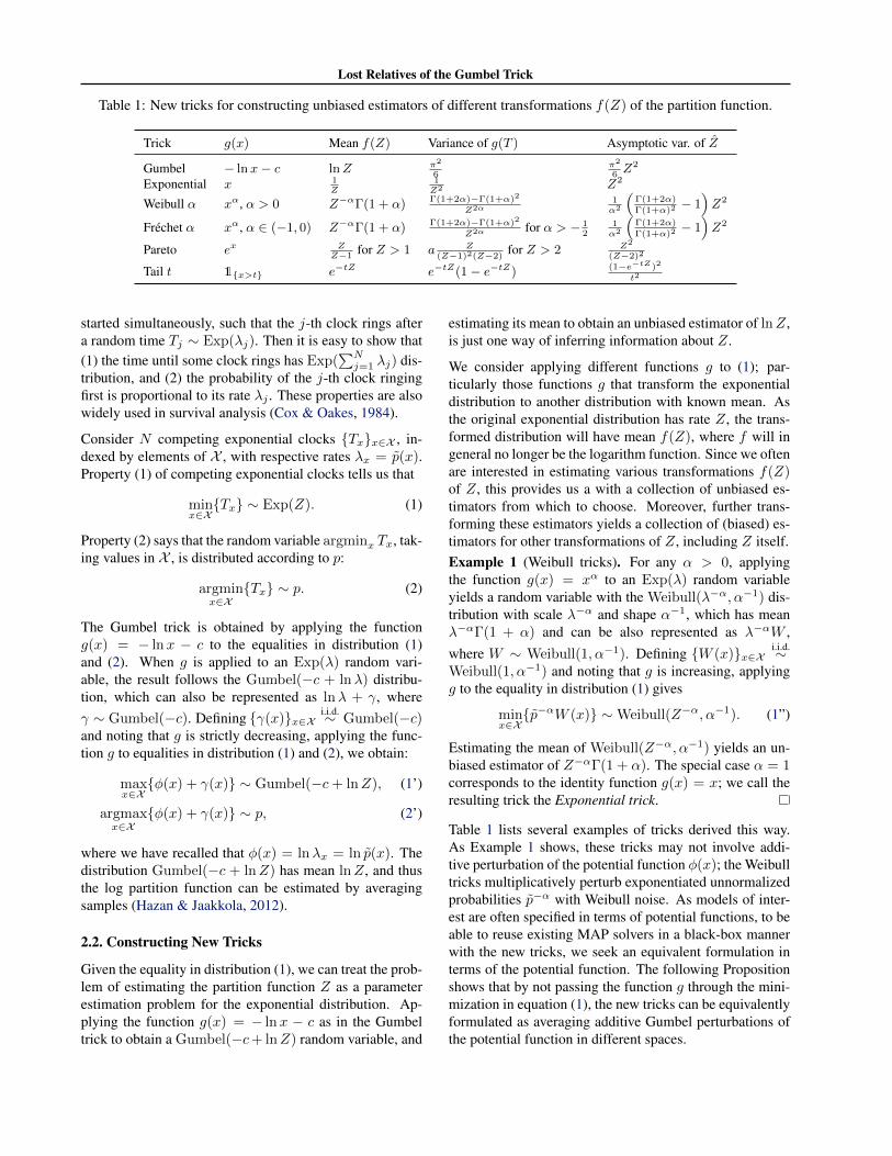
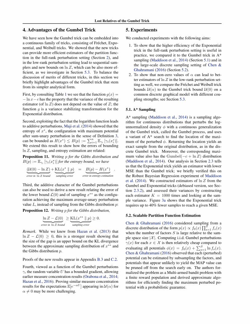
A* sampling (Maddison et al., 2014) is a sampling algo-rithm for continuous distributions that perturbs the log-unnormalized density φ with a continuous generalizationof the Gumbel trick, called the Gumbel process, and usesa variant of A* search to find the location of the maxi-mum of the perturbed φ. Returning the location yields anexact sample from the original distribution, as in the dis-crete Gumbel trick. Moreover, the corresponding maxi-mum value also has the Gumbel(−c + lnZ) distribution(Maddison et al., 2014). Our analysis in Section 2.3 tellsus that the Exponential trick yields an estimator with lowerMSE than the Gumbel trick; we briefly verified this onthe Robust Bayesian Regression experiment of Maddisonet al. (2014). We constructed estimators of lnZ from theGumbel and Exponential tricks (debiased version, see Sec-tion 2.3.2), and assessed their variances by constructingeach estimator K = 1000 times and looking at the sam-ple variance. Figure 3a shows that the Exponential trickrequires up to 40% fewer samples to reach a given MSE.

5.2. Scalable Partition Function Estimation

Chen & Ghahramani (2016) considered sampling from adiscrete distribution of the form p(x) ∝ f0(x)

∏Ss=1 fs(x)

when the number of factors S is large relative to the sam-ple space size |X |. Computing i.i.d. Gumbel perturbationsγ(x) for each x ∈ X is then relatively cheap compared toevaluating all potentials φ(x) = f0(x) +

∑Ss=1 ln fs(x).

Chen & Ghahramani (2016) observed that each (perturbed)potential can be estimated by subsampling the factors, andpotentials that appear unlikely to yield the MAP value canbe pruned off from the search early on. The authors for-malized the problem as a Multi-armed bandit problem witha finite reward population and derived approximate algo-rithms for efficiently finding the maximum perturbed po-tential with a probabilistic guarantee.


10-210-1100

desired MSE (lower to the right)

0

20

40

60

80

100

requir

ed n

um

ber

of

sam

ple

s M Gumbel

Exponential

(a)

0.2 0.0 0.2 0.4 0.6 0.8 1.0 1.2 1.4

trick parameter α

10-2

MSE o

f est

imato

r of

lnZ

Gum

bel tr

ick

Exponenti

al tr

ick

δ= 0. 001

δ= 0. 01

δ= 0. 1

(b)

Figure 3: (a) Sample sizeM required to reach a given MSE usingGumbel and Exponential trick estimators of lnZ, using samplesfrom A∗ sampling (see Section 5.1) on a Robust Bayesian Re-gression task. The Exponential trick is more efficient, requiringup to 40% fewer samples to reach a given MSE. (b) MSE of lnZestimators for different values of α, using M = 100 samplesfrom the approximate MAP algorithm discussed in Section 5.2,with different error bounds δ. For small δ, the Exponential trickis close to optimal, matching the analysis of Section 2.3.2. Forlarger δ, the Weibull trick interpolation between the Gumbel andExponential tricks can provide an estimator with lower MSE.

While Chen & Ghahramani (2016) considered sampling,by modifying their procedure to return the value of themaximum perturbed potential rather than the argmax (cfequations (1) and (2)), we can estimate the partition func-tion instead. However, the approximate algorithm onlyguarantees to find the MAP configuration with a proba-bility 1 − δ. Figure 3b shows the results of running theRacing-Normal algorithm of Chen & Ghahramani (2016)on the synthetic dataset considered by the authors with the“very hard” noise setting σ = 0.1. For low error bounds δthe Exponential trick remained close to optimal, but for alarger error bound the Weibull trick interpolation betweenthe Gumbel and Exponential tricks proved useful to providean estimator with lower MSE.

5.3. Low-rank Perturbation Bounds on lnZ

Hazan & Jaakkola (2012) evaluated tightness of the Gum-bel trick upper bound U(0) ≥ lnZ on 10× 10 binary spinglass models. We show one can obtain more accurate es-timates of lnZ on such models by choosing α 6= 0. Toaccount for the fact that in practice an expectation in U(α)is replaced with a sample average, we treat U(α) as an esti-mator of lnZ with asymptotic bias equal to the bound gap(U(α)− lnZ), and estimate its MSE.

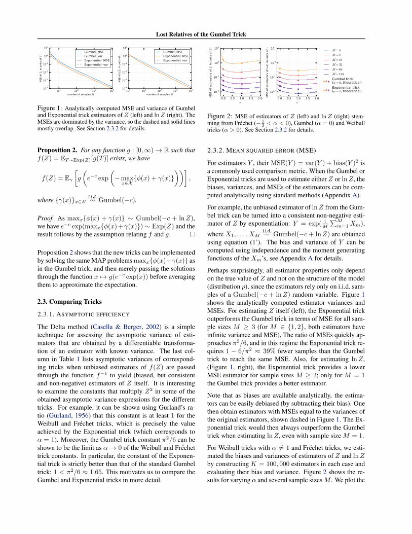
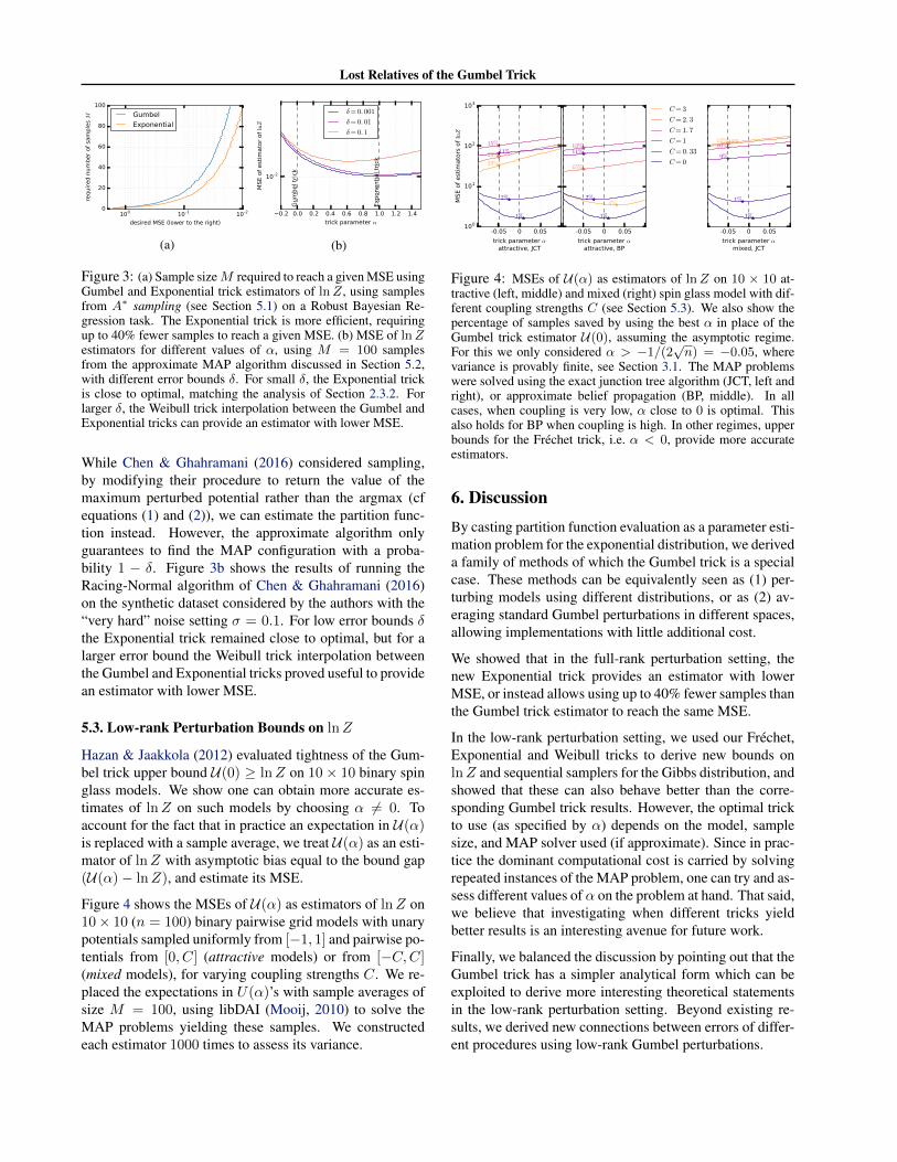
Figure 4 shows the MSEs of U(α) as estimators of lnZ on10× 10 (n = 100) binary pairwise grid models with unarypotentials sampled uniformly from [−1, 1] and pairwise po-tentials from [0, C] (attractive models) or from [−C,C](mixed models), for varying coupling strengths C. We re-placed the expectations in U(α)’s with sample averages ofsize M = 100, using libDAI (Mooij, 2010) to solve theMAP problems yielding these samples. We constructedeach estimator 1000 times to assess its variance.

-0.05 0 0.05

trick parameter αattractive, JCT

100

101

102

103

MSE o

f est

imato

rs o

f lnZ

1%

2%

11%

15%

23%

29%

C= 3

C= 2. 3

C= 1. 7

C= 1

C= 0. 33

C= 0

-0.05 0 0.05

trick parameter αattractive, BP

1%

2%

11%13%

15%

4%

-0.05 0 0.05

trick parameter αmixed, JCT

1%

1%

9%

10%11%12%

Figure 4: MSEs of U(α) as estimators of lnZ on 10 × 10 at-tractive (left, middle) and mixed (right) spin glass model with dif-ferent coupling strengths C (see Section 5.3). We also show thepercentage of samples saved by using the best α in place of theGumbel trick estimator U(0), assuming the asymptotic regime.For this we only considered α > −1/(2

√n) = −0.05, where

variance is provably finite, see Section 3.1. The MAP problemswere solved using the exact junction tree algorithm (JCT, left andright), or approximate belief propagation (BP, middle). In allcases, when coupling is very low, α close to 0 is optimal. Thisalso holds for BP when coupling is high. In other regimes, upperbounds for the Frechet trick, i.e. α < 0, provide more accurateestimators.

6. DiscussionBy casting partition function evaluation as a parameter esti-mation problem for the exponential distribution, we deriveda family of methods of which the Gumbel trick is a specialcase. These methods can be equivalently seen as (1) per-turbing models using different distributions, or as (2) av-eraging standard Gumbel perturbations in different spaces,allowing implementations with little additional cost.

We showed that in the full-rank perturbation setting, thenew Exponential trick provides an estimator with lowerMSE, or instead allows using up to 40% fewer samples thanthe Gumbel trick estimator to reach the same MSE.

In the low-rank perturbation setting, we used our Frechet,Exponential and Weibull tricks to derive new bounds onlnZ and sequential samplers for the Gibbs distribution, andshowed that these can also behave better than the corre-sponding Gumbel trick results. However, the optimal trickto use (as specified by α) depends on the model, samplesize, and MAP solver used (if approximate). Since in prac-tice the dominant computational cost is carried by solvingrepeated instances of the MAP problem, one can try and as-sess different values of α on the problem at hand. That said,we believe that investigating when different tricks yieldbetter results is an interesting avenue for future work.

Finally, we balanced the discussion by pointing out that theGumbel trick has a simpler analytical form which can beexploited to derive more interesting theoretical statementsin the low-rank perturbation setting. Beyond existing re-sults, we derived new connections between errors of differ-ent procedures using low-rank Gumbel perturbations.


AcknowledgementsThe authors thank Tamir Hazan for helpful discussions,and Mark Rowland, Maria Lomeli, and the anonymousreviewers for helpful comments. AW acknowledges sup-port by the Alan Turing Institute under EPSRC grantEP/N510129/1, and by the Leverhulme Trust via the CFI.

ReferencesBelanger, D., Sheldon, D., and McCallum, A. Marginal inference

in MRFs using Frank-Wolfe. In NIPS Workshop on GreedyOptimization, Frank-Wolfe and Friends, 2013.

Bertasius, G., Liu, Q., Torresani, L., and Shi, J. Local Perturb-and-MAP for Structured Prediction. In AISTATS, 2017.

Boykov, Y., Veksler, O., and Zabih, R. Fast approximate energyminimization via graph cuts. IEEE Transactions on patternanalysis and machine intelligence, 23(11):1222–1239, 2001.

Casella, G. and Berger, R. Statistical inference, volume 2.Duxbury Pacific Grove, CA, 2002.

Chen, Y. and Ghahramani, Z. Scalable discrete sampling as amulti-armed bandit problem. In ICML, 2016.

Cox, D. and Oakes, D. Analysis of survival data, volume 21. CRCPress, 1984.

Darbon, J. Global optimization for first order Markov randomfields with submodular priors. Discrete Applied Mathematics,157(16):3412 – 3423, 2009.

Ermon, S., Sabharwal, A., and Selman, B. Taming the curse ofdimensionality: Discrete integration by hashing and optimiza-tion. In ICML, 2013.

Gurland, J. An inequality satisfied by the Gamma function. Scan-dinavian Actuarial Journal, 1956(2):171–172, 1956.

Hazan, T. and Jaakkola, T. On the partition function and randommaximum a-posteriori perturbations. In ICML, 2012.

Hazan, T., Maji, S., and Jaakkola, T. On sampling from the Gibbsdistribution with random maximum a-posteriori perturbations.In NIPS. 2013.

Hazan, T., Orabona, F., Sarwate, A., Maji, S., and Jaakkola,T. High dimensional inference with random maximum a-posteriori perturbations. CoRR, abs/1602.03571, 2016.

Kim, C., Sabharwal, A., and Ermon, S. Exact sampling with in-teger linear programs and random perturbations. In AAAI, pp.3248–3254, 2016.

Kolmogorov, V. Convergent tree-reweighted message passing forenergy minimization. IEEE transactions on pattern analysisand machine intelligence, 28(10):1568–1583, 2006.

Krishnan, Rahul G, Lacoste-Julien, Simon, and Sontag, David.Barrier Frank-Wolfe for Marginal Inference. In NIPS. 2015.

Lauritzen, S. Graphical models. Oxford statistical science series.Clarendon Press, Oxford, 1996. Autre tirage : 1998.

Maddison, C. A Poisson process model for Monte Carlo. InHazan, T., Papandreou, G., and Tarlow, D. (eds.), Perturbation,Optimization, and Statistics. MIT Press, 2016.

Maddison, C., Tarlow, D., and Minka, T. A∗ sampling. In NIPS.2014.

Maji, S., Hazan, T., and Jaakkola, T. Active boundary annotationusing random MAP perturbations. In AISTATS, 2014.

Mooij, J. libDAI: A free and open source C++ library for dis-crete approximate inference in graphical models. Journal ofMachine Learning Research, 11, 2010.

Orabona, F., Hazan, T., Sarwate, A., and Jaakkola, T. On measureconcentration of random maximum a-posteriori perturbations.In ICML, 2014.

Papandreou, G. and Yuille, A. Gaussian sampling by local pertur-bations. In NIPS. 2010.

Papandreou, G. and Yuille, A. Perturb-and-MAP random fields:Using discrete optimization to learn and sample from energymodels. In Proc. IEEE Int. Conf. on Computer Vision (ICCV),pp. 193–200, November 2011.

Tarlow, D., Adams, R., and Zemel, R. Randomized optimummodels for structured prediction. In AISTATS, 2012.

Wainwright, M. and Jordan, M. Graphical Models, Exponen-tial Families, and Variational Inference. Found. Trends Mach.Learn., 1(1-2):1–305, January 2008.

Weller, A. and Domke, J. Clamping improves TRW and meanfield approximations. In AISTATS, 2016.

Weller, A. and Jebara, T. Approximating the Bethe partition func-tion. In UAI, 2014a.

Weller, A. and Jebara, T. Clamping variables and approximateinference. In NIPS, 2014b.

Wright, S. and Nocedal, J. Numerical optimization. SpringerScience, 35:67–68, 1999.

Zhao, J., Djolonga, J., Tschiatschek, S., and Krause, A. Variableclamping for optimization-based inference. In NIPS Workshopon Advances in Approximate Bayesian Inference, December2016.


APPENDIX: Lost Relatives of the Gumbel TrickHere we provide proofs for the results stated in the main text, together with additional supporting lemmas required forthese proofs.

A. Comparison of Gumbel and Exponential tricksIn Section 2.3.1 we analyzed the asymptotic efficiency of different estimators of Z by measuring their asymptotic variance.(As all our estimators in the full-rank perturbation setting are consistent, their bias is 0 in the limit of infinite data, and sothis asymptotic variance equals the asymptotic MSE.) In the non-asymptotic regime, where an estimator Z is constructedfrom a finite set of M samples, we can analyze both the variance var(Z) and the bias (E[Z]− Z) of the estimator. Whilein most cases these cannot be obtained analytically and there we can resort to an empirical evaluation, for the estimatorsstemming from the Gumbel and Exponential tricks analytical treatment turns out to be possible using standard methods.

A.1. Estimating Z

Gumbel trick The Gumbel trick yields an unbiased estimator for lnZ, and we can turn it into a consistent estimator ofZ by exponentiating it:

Z := exp

(1

M

M∑m=1

Xm

)where X1, . . . , XM

iid∼ Gumbel(−c+ lnZ).

Recalling that the moment generating function of a Gumbel(µ) distribution is G(t) = Γ(1− t)eµt, we can obtain by usingindependence of the samples:

E[Z] =

M∏m=1

E[eXm/M ] =(

Γ(1− 1/M)e(lnZ−c)/M)M

= Γ(1− 1/M)Me−cZ,

E[Z2] =

M∏m=1

E[e2Xm/M ] =(

Γ(1− 2/M)e2(lnZ−c)/M)M

= Γ(1− 2/M)Me−2cZ2.

Therefore the squared bias, variance and MSE of the estimator Z are, respectively:

bias(Z)2 = (E[Z]− Z)2 = Z2(Γ(1− 1/M)Me−c − 1

),

var(Z) = E[Z2]− E[Z]2 = Z2(Γ(1− 2/M)Me−2c − Γ(1− 1/M)2Me−2c

),

MSE(Z) = bias(Z)2 + var(Z) = Z2(Γ(1− 2/M)Me−2c − 2Γ(1− 1/M)Me−c + 1

).

These formulas hold for M > 2 where the moment generating functions are defined. For M = 1 the estimator has infinitebias (and infinite variance), and for M = 2 it has infinite variance. Figure 1 (left) shows the functional dependence ofMSE(Z) on the number of samples M ≥ 3, in units of Z2.

Exponential trick The Exponential trick yields an unbiased estimator of 1/Z, and we can turn it into a consistentestimator of Z by inverting it:

Z :=

(1

M

M∑m=1

Xm

)−1

where X1, . . . , XMiid∼ Exp(Z).

As X1, . . . , XM are independent and exponentially distributed with identical rates Z, their sum follows the Gamma distri-bution with shape M and rate Z. Therefore the estimator Z can be written as Z = MY , where Y ∼ InvGamma(M,Z).


Recalling the mean and variance of the Inverse-Gamma distribution, we obtain:

bias(Z)2 = (E[Z]− Z)2 = Z2

(M

M − 1− 1

)= Z2 1

M − 1,

var(Z) = Z2M2 1

(M − 1)2(M − 2),

MSE(Z) = bias(Z)2 + var(Z) = Z2 M − 2 +M2

(M − 1)2(M − 2)= Z2 M + 2

(M − 1)(M − 2).

Again these formulas hold for M > 2 where the relevant expectations are defined: for M = 1 the estimator has infinitebias, and for M ∈ {1, 2} it has infinite variance. Figure 1 (left) shows the functional dependence of MSE(Z) on thenumber of samples M ≥ 3, in units of Z2. By inspecting the curves we observe that the Gumbel trick estimator requiresroughly 45% more samples to yield the same MSE as the Exponential trick estimator.

A.2. Estimating lnZ

A similar analysis can be performed for estimating lnZ rather than Z. In that case the Gumbel trick estimator of lnZ isunbiased and has variance (and thus MSE) equal to 1

Mπ2

6 . On the other hand, the Exponential trick estimator is

lnZ = − ln

(1

M

M∑m=1

Xm

)where X1, . . . , XM

iid∼ Exp(Z).

Again∑Mm=1Xm ∼ Gamma(M,Z) and by reference to properties of the Gamma distribution,

bias(lnZ)2 = (E[Z]− Z)2 = (lnM − (ψ(M)− lnZ)− lnZ)2

= (lnM − ψ(M))2,

var(lnZ) = ψ1(M),

MSE(lnZ) = bias(lnZ)2 + var(lnZ) = (lnM − ψ(M))2

+ ψ1(M),

where ψ(·) is the digamma function and ψ1(·) is the trigamma function. Note that the estimator can be debiased bysubtracting its bias (lnM − ψ(M)). Figure 1 (right) compares the MSE of the Gumbel and Exponential trick estimatorsof lnZ. We observe that the Gumbel trick estimator performs better only for M = 1, and even in that case the Exponentialtrick estimator is better when debiased.

B. Sum-unary perturbationsRecall that sum-unary perturbations refer to the setting where each variable’s unary potentials are perturbed with Gumbelnoise, and the perturbed potential of a configuration sums the perturbations from all variables (see Definition 3 in themain text). Using sum-unary perturbations we can derive a family U(α) of upper bounds on the log partition function(Proposition 4) and construct sequential samplers for the Gibbs distribution (Algorithm 1). Here we provide proofs for therelated results stated in Sections 3.1 and 3.2.

Notation We will write powβ x for xβ , where x, β ∈ R, when we find this increases clarity of our exposition.

Lemma 13 (Weibull and Frechet tricks). For any finite set Y and any function h, we have

pow−α

∑y∈Y

pow−1/α

h(y) = EW[miny

{h(y)

W (y)

Γ(1 + α)

}]where {W (y)}y∈Y

i.i.d.∼ Weibull(1, α−1) for α ∈ (0,∞),

pow−α

∑y∈Y

pow−1/α

h(y) = EF[maxy

{h(y)

F (y)

Γ(1 + α)

}]where {F (y)}y∈Y

i.i.d.∼ Frechet(1,−α−1) for α ∈ (−1, 0).

Proof. This follows from setting up competing exponential clocks with rates λy = h(y)−1/α and then applying the func-tion g(x) = xα as in Example 1 for the case of the Weibull trick. The case of the Frechet trick is similar, except that g isstrictly decreasing for α ∈ (−1, 0), hence the maximization in place of the minimization.


B.1. Upper bounds on the partition function

Proposition 4. For any α ∈ (−1, 0) ∪ (0,∞), the upper bound lnZ ≤ U(α) holds with

U(α) := nln Γ(1 + α)

α+ nc− 1

αlnEγ

[e−αU

].

Proof. We show the result for α ∈ (0,∞) using the Weibull trick; the case of α ∈ (−1, 0) can be proved similarly usingthe Frechet trick. The idea is to prove by induction on n that Z−α ≥ e−αU(α), so that the claimed result follows byapplying the monotonically decreasing function x 7→ − ln(x)/α.

The base case n = 1 is the Clamping Lemma 7 below with j = n = 1. Now assume the claim for n − 1 ≥ 1 and forxn ∈ Xn define

Un−1(α, x1) := (n− 1)ln Γ(1 + α)

α+ (n− 1)c− 1

αlnEγ

[exp

(−α max

x2,...,xn

{φ(x) +

n∑i=2

γi(xi)

})].

With this definition, the Clamping Lemma with j = 1 states that∑x1

pow−1/α e−αUn−1(α,x1) ≤ pow−1/α e

−αU(α), so:

Z−α ≥ pow−α

∑x1∈X1

pow−1/α

e−αUn−1(α,x1) [inductive hypothesis]

≥ pow−α

pow−1/α

e−αU(α) [Clamping Lemma]

= e−αU(α),

as required to complete the inductive step.

Proposition 5. The limit of U(α) as α→ 0 exists and equals U(0) := E[U ], i.e. the Gumbel trick upper bound.

Proof. Recall that U(α) = n ln Γ(1+α)α + nc − 1

α lnE[e−αU

]. The first term tends to nψ(1) = −cn as α → 0 by

L’Hopital’s rule, where ψ is the digamma function. The second term is constant in α. In the last term, E[e−αU

]is the

moment generating function of U evaluated at −α, and as such its derivative at α = 0 exists and equals the negative of themean of U . Hence by L’Hopital’s rule,

− limα→0

1

αlnE

[e−αU

]= − lim

α→0

−E[U ]

E [e−αU ]= E[U ] = U(0).

The claimed result then follows by the Algebra of Limits, as the contributions of the first two terms cancel.

Proposition 6. The function U(α) is differentiable at α = 0 and the derivative equals

d

dαU(α)

∣∣∣∣α=0

= nπ2

12− var(U)

2.

Proof. First we show that U(α) is differentiable on (−1, 0) ∪ (0,∞), and that the limit of the derivative as α → 0 existsand equals nπ2/12− var(U)/2.

The first term of U(α) is n ln Γ(1+α)α , which is differentiable for α ∈ (−1, 0) ∪ (0,∞) by the Quotient Rule, and its

derivative equalsd

dαn

ln Γ(1 + α)

α= n

ψ(1 + α)α− ln Γ(1 + α)

α2,

where ψ is the digamma function (logarithmic derivative of the gamma function). Applying L’Hopital’s rule we note that

limα→0

d

dαn

ln Γ(1 + α)

α= n lim

α→0

ψ(1 + α) + αψ(1)(1 + α)− ψ(1 + α)

2α= n

ψ(1)(1)

2= n

ζ(2)

2= n

π2

12,


where ψ(1) is the trigamma function (derivative of the digamma function), whose value at 1 is known to be ζ(2) = π2/6,the Riemann zeta function evaluated at 2.

The second term of U(α) is constant in α. The last term can be written as K(−α)/(−α), where K is the cumulantgenerating function (logarithm of the moment generating function) of the random variable U . The cumulant generatingfunction is differentiable, and by the Quotient rule

d

dα

K(−α)

−α= −αK

′(−α)−K(−α)

α2.

Applying L’Hopital’s rule we note that

limα→0

d

dα

K(−α)

−α= limα→0

K ′(−α) + αK ′′(−α)−K ′(−α)

2α=K ′′(0)

2=

var(U)

2,

where we have used that the second derivative of the cumulant generating function is the variance.

As U(α) is continuous at 0 by construction, the above implies that it has left and right derivatives at 0. As the values ofthese derivatives coincide, the function is differentiable at 0 and the derivative has the stated value.

Recall that for a variable index j ∈ {1, . . . , n} we also defined partial sum-unary perturbations

Uj(x1, . . . , xj−1) := maxxj ,...,xn

φ(x) +

n∑i=j

γi(xi)

,

which fix the variables x1, . . . , xj−1 and perturb the remaining ones.Lemma 7 (Clamping Lemma). For any j ∈ {1, . . . , n} and any fixed partial variable assignment (x1, . . . , xj−1) ∈X1 × · · · × Xj−1, the following inequality holds with any trick parameter α ∈ (−1, 0) ∪ (0,∞):∑

xj∈Xj

Eγ[e−(n−j) ln Γ(1+α)−α(n−j)c)e−αUj+1(x1,...,xj)

]−1/α

≤ Eγ[e−(n−(j−1)) ln Γ(1+α)−α(n−(j−1))c)e−αUj(x1,...,xj−1)

]−1/α

.

Proof. For α > 0, from the Weibull trick (Lemma 13), using independence of the perturbations and Jensen’s inequality,

pow−α

∑xj∈Xj

pow−1/α

EW

minxj+1,...,xn

p(x)−αn∏

i=j+1

W (xi)

Γ(1 + α)

= EW

minxj∈Xj

EW

minxj+1,...,xn

p(x)−αn∏

i=j+1

W (xi)

Γ(1 + α)

W (xj)

Γ(1 + α)

≤ EW

minxj ,...,xn

p(x)−αn∏i=j

W (xi)

Γ(1 + α)

Representing the Weibull random variables in terms of Gumbel random variables using the transformation W = e−(γ+c)α,where γ ∼ Gumbel(−c), and manipulating the obtained expressions yields the claimed result.


B.2. Sequential samplers for the Gibbs distribution

The family of sequential samplers for the Gibbs distribution presented in the main text as Algorithm 1 has the same overallstructure as the sequential sampler derived by Hazan et al. (2013) from the Gumbel trick upper bound U(0), and hencecorrectness can be argued similarly. Conditioned on accepting the sample, the probability that x = (x1, . . . , xn) is returnedis

n∏i=1

pi(xi) =

n∏i=1

e−c

Γ(1 + α)1/α

Eγ[e−αUi+1(x1,...,xi)

]−1/α

Eγ[e−αUi(x1,...,xi−1)

]−1/α=

e−nc

Γ(1 + α)n/α

(e−αφ(x1,...,xn)

)−1/α

E[e−αU ]−1/α∝ p(x),

as required to show that the produced samples follow the Gibbs distribution p. Note, however, that in practice one intro-duces an approximation by replacing expectations with sample averages.

B.3. Relationship between errors of sum-unary Gumbel perturbations

We write x∗ for the (random) MAP configuration after sum-unary perturbation of the potential function, i.e.,

x∗ := argmaxx∈X

{φ(x) +

n∑i=1

γi(xi)

}.

Let qsum(x) := P[x = x∗] be the probability mass function of x∗.

The following results links together the errors acquired when using summed unary perturbations to upper bound the logpartition function lnZ ≤ U(0) using the Gumbel trick upper bound by Hazan & Jaakkola (2012), to approximately samplefrom the Gibbs distribution by using qsum instead, and to upper bound the entropy of the approximate distribution qsumusing the bound due to Maji et al. (2014).Proposition 11. Writing p for the Gibbs distribution, we have

(U(0)− lnZ)︸︷︷︸error in lnZ bound

+ KL(qsum ‖ p)︸︷︷︸sampling error

= Eγi [γi(x∗i )]−H(qsum)︸︷︷︸

error in entropy estimation

.

Proof. By conditioning on the maximizing configuration x∗, we can rewrite the Gumbel trick upper bound U(0) as follows:

U(0) = Eγ

[maxx∈X

{θ(x) +

n∑i=1

γi(xi)

}]

=∑x∈X

qsum(x)

(θ(x) + Eγ

[n∑i=1

γi(xi) | x = x∗

])

=∑x∈X

qsum(x)θ(x) +

n∑i=1

Eγi [γi(x∗i )] .

At the same time, the KL divergence between qsum and the Gibbs distribution p generally expands as

KL(qsum ‖ p) = −H(qsum)−∑x∈X

qsum(x) lnexp (θ(x))∑

x∈X exp (θ(x))

= −H(qsum)−∑x∈X

qsum(x)θ(x) + lnZ.

Adding the two equations together and rearranging yields the claimed result.


C. Averaged unary perturbationsC.1. Lower bounds on the partition function

In the main text we stated the following two lower bounds on the log partition function lnZ.Proposition 9. Let α ∈ (−1, 0) ∪ (0,∞). For any subset S ⊆ {1, . . . , n} of the variables x1, . . . , xn we have lnZ ≥

c+ln Γ(1 + α)

α− 1

αlnE

[e−αmaxx{φ(x)+γS(xS)}

],

where xS := {xi : i ∈ S} and γS(xS) ∼ Gumbel(−c) independently for each setting of xS .

Proof. Let S := {1, . . . , n} \ S. First we handle the case α > 0. We have trivially that

pow−α Z = pow−α∑xS

∑xS

eφ(xS ,xS) ≤ pow−α∑xS

maxxS

eφ(xS ,xS).

The Weibull trick tells us that pow−α∑y pow−1/α h(y) = EW [miny

h(y)Γ(1+α)W (y)] where {W (y)}y

iid∼ Weibull(1, α−1).Applying this to the summation over xS on the right-hand side of the above inequality, we obtain

pow−α Z ≤ EW

[minxS

pow−α maxxS eφ(xS ,xS)

Γ(1 + α)W (xS)

].

Expressing the Weibull random variable W (xS) as e−α(γS(xS)+c) with γS(xS) ∼ Gumbel(−c), the right-hand side canbe simplified as follows:

pow−α Z ≤1

Γ(1 + α)Eγ[pow−α max

xSmaxxS

eφ(xS ,xS)eγS(xS)+c

]=

e−αc

Γ(1 + α)Eγ[exp

(−αmax

x{φ(x) + γS(xS)}

)].

Taking the logarithm and dividing by −α < 0 yields the claimed result for positive α. For α ∈ (−1, 0) we proceedsimilarly, obtaining that

pow−α Z ≥ pow−α∑xS

maxxS

eφ(xS ,xS)

= EF

[minxS

pow−α maxxS eφ(xS ,xS)

Γ(1 + α)F (xS)

],

where F (x(S)) ∼ Frechet(1,−α−1). Representing these random variables as e−α(γS(xS)+c) with γS(xS) ∼Gumbel(−c), simplifying as in the previous case and finally dividing the inequality by −α > 0 yields the claimed re-sult for α ∈ (−1, 0).

Corollary 10. For any α ∈ (−1, 0) ∪ (0,∞), we have the lower bound lnZ ≥ L(α), where

L(α) := c+ln Γ(1 + α)

α− 1

nαlnE [exp (−nαL)] ,

Proof. Applying Proposition 9 n times with all singleton sets S = {i} and averaging the obtained lower bounds yields

lnZ ≥ c+ln Γ(1 + α)

α− 1

n

n∑i=1

1

αlnE

[exp

(−αmax

x{φ(x) + γi(xi)}

)]= c+

ln Γ(1 + α)

α− 1

nαlnE

[exp

(−

n∑i=1

αmaxx{φ(x) + γi(xi)}

)]

= c+ln Γ(1 + α)

α− 1

nαlnE

[exp

(−nα 1

n

n∑i=1

maxx{φ(x) + γi(xi)}

)],


where the first equality used the fact that the perturbations γi(xi) are mutually independent for different indices i to replacethe product of expectations with the expectation of the product. The claimed result follows by applying Jensen’s inequalityto swap the summation and the convex maxx function, noting that the inequality works out the right way for both positiveand negative α.

Jensen’s inequality can be used to relate the general lower bound L(α) to the Gumbel trick lower bound L(0), showingthat the former cannot be arbitrarily worse than the latter:

Proposition 14. For all α ∈ (−1, 0), the lower bound L(α) on lnZ satisfies

L(α) ≥ L(0) +ln Γ(1 + α)

α+ c

Proof. Apply Jensen’s inequality with the convex function x 7→ e−nα to the last term in the definition of L(α), noting thatthe inequality works out the stated way for α < 0.

Note that ln Γ(1+α)α + c ≤ 0 for α ∈ (−1, 0) so this result does not imply that the Frechet lower bounds are tighter than the

Gumbel lower bound L(0); it merely says that they cannot be arbitrarily worse than L(0).

C.2. Relationship between errors of averaged-unary Gumbel perturbations

In this section we write x∗ for the (random) MAP configuration after average-unary perturbation of the potential function,i.e.,

x∗ := argmaxx∈X

{φ(x) +

1

n

n∑i=1

γi(xi)

}.

where {γi(xi) | xi ∈ Xi, 1 ≤ i ≤ n}i.i.d.∼ Gumbel(−c). Let qavg(x) := P[x = x∗] be the probability mass function of x∗.

The Gumbel trick lower bound on the log partition function lnZ due to Hazan et al. (2013) is:

lnZ ≥ L(0) = Lφ(0) := Eγ

[minx∈X

{φ(x) +

1

n

n∑i=1

γi(xi)

}]. (3)

We show that the gap of this Gumbel trick lower bound on lnZ upper bounds the KL divergence between the approximatedistribution qavg and the Gibbs distribution p. To this end, we first need an entropy bound for qavg analogous to Theorem 1of (Maji et al., 2014).

Theorem 15. The entropy of qavg can be lower bounded using expected values of max-perturbations as follows:

H(qavg) ≥ 1

n

n∑i=1

Eγi [γi(x∗i )]

Remark. Theorem 1 of (Maji et al., 2014) and this Theorem 15 differ in three aspects: (1) the former is an upper bound andthe latter is a lower bound, (2) the former sums the expectations while the latter averages them, and (3) the distributionsqsum and qavg of x∗ in the two theorems are different.

Proof. By the duality relation between negative entropy and the log partition function (Wainwright & Jordan, 2008), theentropy H(qavg) of the unary-avg perturb-max distribution qavg can be expressed as

H(qavg) = infϕ

{lnZϕ −

∑x∈X

qavg(x)ϕ(x)

},

where the variable ϕ ranges over all potential functions on X , and Zϕ =∑

x∈X expϕ(x). Applying the Gumbel tricklower bound on the log partition function gives

H(qavg) ≥ infϕ

{Lϕ(0)−

∑x∈X

qavg(x)ϕ(x)

},


Proposition 16 in Appendix D shows that Lϕ(0) is a convex function of ϕ. The expression −∑

x∈X q(x)ϕ(x) is a linearfunction of ϕ, so also convex, and thus as a sum of two convex functions, the quantity Lϕ(0) −

∑x∈X q(x)ϕ(x) within

the infimum is a convex function of ϕ. Moreover, Proposition 17 in Appendix D tells us that the partial derivatives can becomputed as

∂

∂ϕ(x)

(Lϕ(0)−

∑x∈X

qavg(x)ϕ(x)

)= qϕ(x)− qavg(x)

where qϕ(x) is the unary-avg perturb-max distribution associated with the potential function ϕ. Proposition 18 in Ap-pendix D confirms that these partial derivatives are continuous, so we observe that as a function of ϕ, the expressionLϕ(0)−

∑x∈X qavg(x)ϕ(x) is a convex function with continuous partial derivatives, so it is a differentiable convex func-

tion. This is sufficient to establish that the point ϕ = φ is a global minimum of this function (Wright & Nocedal, 1999).Hence

H(qavg) ≥ infϕ

{Lϕ(0)−

∑x∈X

qavg(x)ϕ(x)

}= Lφ(0)−

∑x∈X

qavg(x)φ(x)

=∑x∈X

qavg(x)Eγ

[φ(x) +

1

n

n∑i=1

γi(xi) | x = x∗

]−∑x∈X

qavg(x)φ(x)

=1

n

n∑i=1

Eγi [γi(x∗i )]

where we conditioned on the maximizing configuration x∗ when expanding Lφ(0).

Remark. This proof proceeded in the same way as the proof of Maji et al. (2014) for the upper bound, except that es-tablishing the minimizing configuration of the infimum is a non-trivial step that is actually required in this case. Thesecond revision of (Hazan et al., 2016) computes the derivative of Uϕ(0) −

∑x∈X qsum(x)ϕ(x), which is similar to our

Lϕ(0)−∑

x∈X qavg(x)ϕ(x), by differentiating under the expectation.

Equipped with Theorem 15, we can now show a link between the approximation “errors” of the averaged-unary perturba-tion MAP configuration distribution qavg (to the Gibbs distribution p) and estimate L(0) (to lnZ).Proposition 12. Let p be the Gibbs distribution on X . Then

lnZ − L(0)︸︷︷︸error in lnZ bound

≥ KL(qavg ‖ p)︸︷︷︸sampling error

≥ 0

Remark. While we knew from Hazan et al. (2013) that lnZ − L(0) ≥ 0 (i.e. that L(0) is a lower bound on lnZ), thisis a stronger result showing that the size of the gap is an upper bound on the KL divergence between the average-unaryperturbation MAP distribution qavg and the Gibbs distribution p.

Proof. The Kullback-Leibler divergence in question expands as

KL(qavg ‖ p) = −H(qavg)−∑x∈X

qavg(x) lnexpφ(x)∑

x∈X expφ(x)= −H(qavg)−

∑x∈X

qavg(x)φ(x) + lnZ.

From the proof of Theorem 15 we know that H(qavg) ≥ L(0)−∑

x∈X qavg(x)φ(x), so

KL(qavg ‖ p) ≤ −L(0) +∑x∈X

qavg(x)φ(x)−∑x∈X

qavg(x)φ(x) + lnZ = lnZ − L(0).


D. Technical resultsIn this section we write L(φ) instead of Lφ(0) for the Gumbel trick lower bound on lnZ associated with the potentialfunction φ, see equation (3).

Proposition 16. The Gumbel trick lower bound L(φ), viewed as a function of the potentials φ, is convex.

Proof. Convexity can be proved directly from definition. Let φ1 and φ2 be two arbitrary potential functions on a discreteproduct space X , and let λ ∈ [0, 1]. Then

L(λφ1 + (1− λ)φ2)

= Eγ

[maxx∈X

{λφ1(x) + (1− λ)φ2(x) +

1

n

n∑i=1

γi(xi)

}]

= Eγ

[maxx∈X

{λ

(φ1(x) +

1

n

n∑i=1

γi(xi)

)+ (1− λ)

(φ2(x) +

1

n

n∑i=1

γi(xi)

)}]

≤ Eγ

[λmax

x∈X

{φ1(x) +

1

n

n∑i=1

γi(xi)

}+ (1− λ) max

x∈X

{φ2(x) +

1

n

n∑i=1

γi(xi)

}]= λL(φ1) + (1− λ)L(φ2),

where we have used convexity of the max function to obtain the inequality, and linearity of expectation to arrive at the finalequality.

Remark. This convexity proof goes through for other (low-dimensional) perturbations as well, e.g. it also works for Uφ(0).

Proposition 17. The Gumbel trick lower bound L(φ), viewed as a function of the potentials φ, has partial derivatives

∂

∂φ(x)L(φ) = qφ(x)

where qφ is the probability mass function of the average-unary perturbation MAP configuration’s distribution associatedwith the potential function φ.

Proof. Let x ∈ X , so that φ(x) is a general component of φ, and let ex be the indicator vector of x. For any δ ∈ R, thechange in the lower bound L due to replacing φ(x) with φ(x) + δ is

L(φ+ δex)− L(φ) = Eγ

[maxx∈X

{φ(x) + δ1{x = x}+

1

n

n∑i=1

γi(xi)

}]− Eγ

[maxx∈X

{φ(x) +

1

n

n∑i=1

γi(xi)

}]

= Eγ

[maxx∈X

{φ(x) + δ1{x = x}+

1

n

n∑i=1

γi(xi)

}−max

x∈X

{φ(x) +

1

n

n∑i=1

γi(xi)

}]= Eγ [∆(φ, δ, x, γ)]

by linearity of expectation, where we have denoted by ∆(φ, δ, x, γ) the change in maximum due to replacing the potentialφ(x) with φ(x) + δ. Let’s condition on the argmax before modifying φ:

L(φ+ δex)− L(φ) = Eγ [∆(φ, δ, x, γ)] =∑x∈X

qφ(x)Eγ [∆(φ, δ, x, γ) | x is the original argmax]

Now let’s condition on the size of the gap G between the maximum and the runner-up:

Eγ [∆(φ, δ, x, γ) | x is the original argmax] = P(G ≤ |δ|)Eγ [∆(φ, δ, x, γ) | x is the original argmax, G ≤ |δ|]+ P(G > |δ|)Eγ [∆(φ, δ, x, γ) | x is the original argmax, G > |δ|]

Let’s examine all four terms on the right-hand side one by one:


1. P(G ≤ |δ|)→ P(G = 0) = 0 as δ → 0 by monotonicity of measure.2. Eγ [∆(φ, δ, x, γ) | x is the original argmax, G ≤ |δ|] ≤ δ since |∆(φ, δ, x, γ)| ≤ |δ| always holds.3. P(G > |δ|)→ P(G ≥ 0) = 1 as δ → 0 by monotonicity of measure.4. Eγ [∆(φ, δ, x, γ) | x is the original argmax, G > |δ|] = δ1{x = x} since in this case both maximizations in the

definition of ∆(φ, δ, x, γ) are maximized at x.

Therefore, as δ → 0,

Eγ [∆(φ, δ, x, γ) | x is the original argmax] = o(1)o(δ) + (1 + o(1))δ1{x = x}

Putting things together, we have

limδ→0

L(φ+ δex)− L(φ)

δ=∑x∈X

qφ(x) limδ→0

1

δEγ [∆(φ, δ, x, γ) | x is the original argmax]

=∑x∈X

qφ(x)1{x = x}

= qφ(x),

which proves the stated claim directly from definition of a partial derivative.

Proposition 18. The probability mass function qφ of the average-unary perturbation MAP configuration’s distributionassociated with a potential function φ is continuous in φ.

Proof. For any x∗ ∈ X we have from definition

qφ(x∗) = P

[x∗ = argmax

x∈X

{φ(x) +

1

n

n∑i=1

γi(xi)

}]

= P

[φ(x∗) +

1

n

n∑i=1

γi(x∗i ) > max

x∈X\{x∗}

{φ(x) +

1

n

n∑i=1

γi(xi)

}]

= E

[1

{φ(x∗) +

1

n

n∑i=1

γi(x∗i ) > max

x∈X\{x∗}

{φ(x) +

1

n

n∑i=1

γi(xi)

}}]

which is continuous in φ by continuity of max, of 1 {· > ·} (as a function of φ) and by the Bounded Convergence Theorem.

Remark. The results above show that the Gumbel trick lower bound L(φ), viewed as a function of the potentials φ, isconvex and has continuous partial derivatives.

lost relatives of the gumbel trick - matej...

Documents