magnetizing currents in power transformers – measurements ...1106261/fulltext02.pdf · of the...
TRANSCRIPT

KTH Electrical Engineering
Magnetizing Currents in Power Transformers – Measurements, Simulations,
and Diagnostic Methods
Claes Carrander
Doctoral Thesis Stockholm, Sweden 2017

TRITA-EE 2017:042 ISBN: 978-91-7729-417-7 ISSN: 1653-5146
Elektroteknisk teori och konstruktion
Kungliga Tekniska Högskolan SE-100 44 Stockholm
SWEDEN Akademisk avhandling som med tillstånd av Kungliga Tekniska Högskolan framläggs till offentlig granskning för avläggande av teknologie doktorsexamen torsdagen den 31 augusti klockan 10.00 i sal F3, Kungliga Tekniska Högskolan, Lindstedtsvägen 26, Stockholm. © Claes Carrander, 2017 Tryck: Universitetsservice US-AB

i
Abstract
Power transformers are a vital part of the modern power grid, and much attention is devoted to keeping them in optimum shape. For the core, however, effective diagnostic methods are scarce. The reason for this is primarily that transformer cores are non-linear and therefore difficult to model. Additionally, they are usually quite stable and can operate for decades without any apparent aging. Nevertheless, transformer cores have been known to malfunction, and even melt. Considering the cost of a core malfunction, a method of predicting and preventing such failures would be beneficial. Deeper understanding of the core would also allow manufacturers to improve their transformers.
This thesis demonstrates a method for transformer core diagnostics. The method uses the no-load current of the transformer as an indicator, and gives different characteristic signatures for different types of faults or defects. Using the no-load current for the diagnostic gives high sensitivity. The method is therefore able to detect defects that are too small to have an impact on the losses. In addition to different types of fault, the method can in some cases also distinguish between faults in different locations within the core.
Both single-phase and three-phase transformers can be diagnosed using this method, and the measurements can be easily performed at any facility capable of measuring the no-load loss. There are, however, some phenomena that occur in large transformers, and in transformers with high rated voltages. Examples include capacitive resonance and magnetic remanence. This thesis proposes and demonstrates techniques for compensating for these phenomena. With these compensating techniques, the repeatability of the measurements is high. It is shown that units with the same core steel tend to have very similar no-load behavior.
The diagnostics can then be performed either by comparing the transformer to another unit, or to simulations. The thesis presents one possible

ii
simulation method, and demonstrates the agreement with measurements. In most units, the no-load currents can be reproduced to within 10 % - 20 %.
This topological simulation method includes both the electric circuit and an accurate model of the magnetic hysteresis. It is therefore also suitable for other, related, studies in addition to core diagnostics. Possible subjects include ferroresonance, inrush, DC magnetization of transformers, and transformer core optimization.
The thesis also demonstrates that, for three-phase transformers, it is possible to compare the phases to each other. This technique makes it possible to diagnose a transformer even without a previous measurement to compare to, and without the data required to make a simulation.

iii
Sammanfattning
Krafttranformatorer utgör en vital del av dagens kraftnät. Mycket tid och möda läggs därför på service och underhåll för att hålla dem i bästa möjliga skick. Det är dock ont om verktyg för diagnostik av transformatorkärnor. Detta beror huvudsakligen på att transformatorkärnor är ickelinjära och därför svåra att modellera. Dessutom är de vanligtvis stabila och åldras inte i någon större utsträckning. Trots detta händer det att fel uppstår i transformatorkärnor. I extrema fall kan till och med delar av kärnan smälta. Med tanke på kostnaden för att ersätta en havererad transformator så vore det därför fördelaktigt att utveckla en metod för att förutse och förebygga sådana fel. En djupare förståelse för kärnan i stort skulle också vara till hjälp i arbetet med att utveckla allt bättre transformatorer.
Denna avhandling demonstrerar en diagnostikmetod för transformator-kärnor. Metoden använder tomgångsströmmen som en indikator, och olika typer av kärnfel ger olika karakteristiska signaler. Tomgångsströmmen är känslig för ändringar i kärnan. Det är därför möjligt, med den här metoden, att detektera kärnfel som är för små för att påverka tomgångsförlusterna. Utöver att skilja på olika typer av kärnfel, så kan metoden i vissa fall även skilja på olika felställen.
Både enfas- och trefastransformatorer kan diagnosticeras på det här sättet, och mätningarna är lätta att utföra så länge transformatorn kan tomgångsmagnetiseras. Det finns dock några fenomen som uppstår i stora transformatorer med höga märkspänningar, och som måste kompenseras för. I avhandlingen föreslås tekniker för att hantera fenomen som kapacitiv resonans och magnetisk remanens. Med hjälp av dessa tekniker kan repeterbarheten i mätningarna göras hög. Detta visas, bland annat, i att transformatorer med samma kärnmaterial också har väldigt lika tomgångs-beteende.
Själva diagnostiken kan utföras genom att den studerade transformatorn jämförs antingen med en annan enhet, eller med en simulering. En möjlig simuleringsmetod demonstreras i avhandlingen. Jämförelse med

iv
mätresultat visar att metoden kan simulera tomgångsströmmar med en avvikelse på 10 % - 20 % i de flesta enheter.
Denna topologiska simuleringsmetod inkluderar både den elektriska och den magnetiska kretsen. Detta gör den användbar även i andra, liknande, studier. Exempel på sådana områden är ferroresonans, inkopplings-strömmar och DC-magnetisering av transformatorer. Simuleringarna kan även vara till hjälp vid optimering av transformatorkärnor.
Denna avhandling demonstrerar även att diagnostiken, för trefas-transformatorer, kan utföras genom att faserna jämförs med varandra. På så sätt är det möjligt att diagnosticera en transformator även om det inte finns någon liknande enhet att jämföra med, eller och tillräckliga data saknas för att göra en simulering.

v
Acknowledgments
I would like to thank all the people who have been involved in this work, and who have made this thesis possible.
First of all, the project would never have existed without the Kurt Gramm, Tord Bengtsson and Nilanga Abeywickrama from ABB. These men were part of the project before it even was a project, and have contributed with their expertise in all matters.
I would like to thank my sponsors: ELEKTRA and SweGRIDS. In addition to providing economic support, the companies and authorities making up these two organizations have also contributed with knowledge through my reference group. We have had many fruitful discussions, and their input has been invaluable.
For practical matters, I have always turned to Bengt Jönsson and test room personnel at ABB Ludvika. The measurements on which this thesis is based would never have been possible without them.
Then there is everyone at KTH who has helped me with the academic side of the thesis. Teachers, staff, and students have all been important, but I would like to give special thanks to Martin Norgren, who has reviewed my theses and provided valuable input, and to Hans Edin, who has been my official supervisor for the last two years of the thesis. Seyed Ali Mousavi also deserves special thanks for developing the simulation method used in this thesis. He has also continued to be a source for simulation know-how after his dissertation.
I would also like to express my gratitude to the Nippon Steel and Sumitomo Metals Corporation for showing me how electrical steel is made. Dr. Mizokami and Dr. Arai have also been of great help providing measurements and knowledge about electrical steel.
Finally, I would like to acknowledge my supervisor, Göran Engdahl for helping me in both academic and administrative matters during my studies.

vi

vii
Contents Abstract ................................................................................................................ i Sammanfattning ................................................................................................ iii Acknowledgments................................................................................................ v List of symbols ................................................................................................... xi 1 Introduction ................................................................................................. 1
1.1 Background ......................................................................................... 1 1.2 Aim and scientific contribution ......................................................... 5 1.3 Previous publications .........................................................................7 1.4 Thesis outline ..................................................................................... 8
2 Magnetism and power transformers .......................................................... 9 2.1 Notes on terminology and conventions ............................................ 9
2.1.1 The magnetic fields ........................................................................ 9 2.1.2 Magnetizing current and no-load current ................................... 11
2.2 Magnetization of core steels ............................................................. 11 2.2.1 Ferromagnetism and static hysteresis ......................................... 11 2.2.2 Dynamic hysteresis ....................................................................... 18 2.2.3 Anatomy of the hysteresis curve .................................................. 21
2.3 Power transformers ......................................................................... 22 2.3.1 Factors affecting transformer design .......................................... 22 2.3.2 Transformer windings and vector groups .................................. 24 2.3.3 Transformer rating and the per-unit notation ........................... 25 2.3.4 Core geometries ........................................................................... 30 2.3.5 Autotransformers......................................................................... 32 2.3.6 Core steel ...................................................................................... 33 2.3.7 Core construction ......................................................................... 36 2.3.8 The no-load loss test ..................................................................... 41

viii
3 Equipment and measurements ................................................................ 43 3.1 Measurement principle ................................................................... 43 3.2 Data acquisition ............................................................................... 46 3.3 Large power transformers ............................................................... 48 3.4 1 MVA dry-type transformer with simulated faults ........................ 51 3.5 100 kVA distribution transformer .................................................. 53 3.6 Table-top models ............................................................................. 54 3.7 Measurement of steel properties .................................................... 55
4 Measurement results ................................................................................. 61 4.1 Magnetic path length estimation ..................................................... 61 4.2 Single-phase transformers with homogenous cores ...................... 63 4.3 Single-phase transformers with varying core cross-sections ........ 64 4.4 Three-phase transformers ............................................................... 66
5 Transformer simulations .......................................................................... 69 5.1 The Time-Step Topological Model .................................................. 70
5.1.1 TTM algorithm ............................................................................. 74 5.2 Implementation of static hysteresis ................................................ 79 5.3 Implementation of dynamic hysteresis .......................................... 83 5.4 Modeling of the major loop ............................................................. 85
5.4.1 Experimental determination of the fitting parameters ............. 90 5.5 Modeling parallel reluctance elements ........................................... 94 5.6 Initial magnetization and inrush currents ..................................... 95 5.7 Simulation results, single phase...................................................... 97
5.7.1 Anhysteretic magnetization ........................................................ 98 5.7.2 Hysteresis based on SST measurement ..................................... 101 5.7.3 Hysteresis based on approximated major loop ........................ 102 5.7.4 Parallel reluctance elements ..................................................... 103 5.7.5 Air gaps in corner joints ............................................................ 106

ix
5.7.6 The electrical circuit .................................................................. 106 5.7.7 Discussion ................................................................................... 107
5.8 Simulation results, three phase ...................................................... 110 5.8.1 Anhysteretic magnetization in three-phase transformers ......... 111 5.8.2 Rotational magnetization in corner joints ................................ 112 5.8.3 Discussion ................................................................................... 113
6 Magnetizing phenomena in real power transformers ............................ 115 6.1 Phase imbalance.............................................................................. 115 6.2 The impact of delta windings on the no-load current ................... 121 6.3 Remanence in large power transformers ...................................... 123 6.4 Harmonics .......................................................................................126 6.5 Capacitive current and resonance ................................................. 130
6.5.1 Capacitive current compensation .............................................. 134 6.5.2 Measurements ............................................................................ 138 6.5.3 Simulations ................................................................................ 140
7 Core diagnostics ....................................................................................... 145 7.1 Distinguishing different types of faults ......................................... 145
7.1.1 Partial air gaps ............................................................................146 7.1.2 Circulating currents around the whole core cross-section ....... 154 7.1.3 Circulating currents around part of the core cross-section ...... 155
7.2 Diagnosing a core ............................................................................ 161 7.3 Three-phase symmetry ...................................................................162 7.4 Comparison between voltage levels ............................................... 165
8 Further work ............................................................................................ 167 8.1 Development of a diagnostic tool ................................................... 167 8.2 Improvement of the simulation method .......................................169
8.2.1 The program implementation ....................................................169 8.2.2 Impedance modeling .................................................................. 171

x
8.2.3 Magnetic circuit modeling .......................................................... 171 8.2.4 The hysteresis model .................................................................. 172
8.3 Further applications ....................................................................... 173 9 Conclusions .............................................................................................. 175 References ........................................................................................................ 177

xi
List of symbols
Boldface symbols are used to denote vectors or matrices.
Symbol Description Unit
A Area (cross-section) m2
B Flux density T
Ba Applied field (flux density) T
Br Remanent flux density T
Brev Reversal flux density T
Bs Saturation flux density T
C Capacitance F
d Sheet thickness m
e Fitting parameter A/m
E Electric field V/m
Eai Anisotropy energy J
Eex Exchange energy J
Etot Total magnetic energy J
EZ Zeeman energy J
F Magnetomotive force A
fr Resonance frequency Hz
G Geometric factor for dynamic eddy currents 1
H Magnetizing field (H-field) A/m
Hc Coercivity A/m
Hcl Classical eddy current field A/m
Hee Excess eddy current field A/m
Hrev Reversal magnetizing field A/m
I Current A
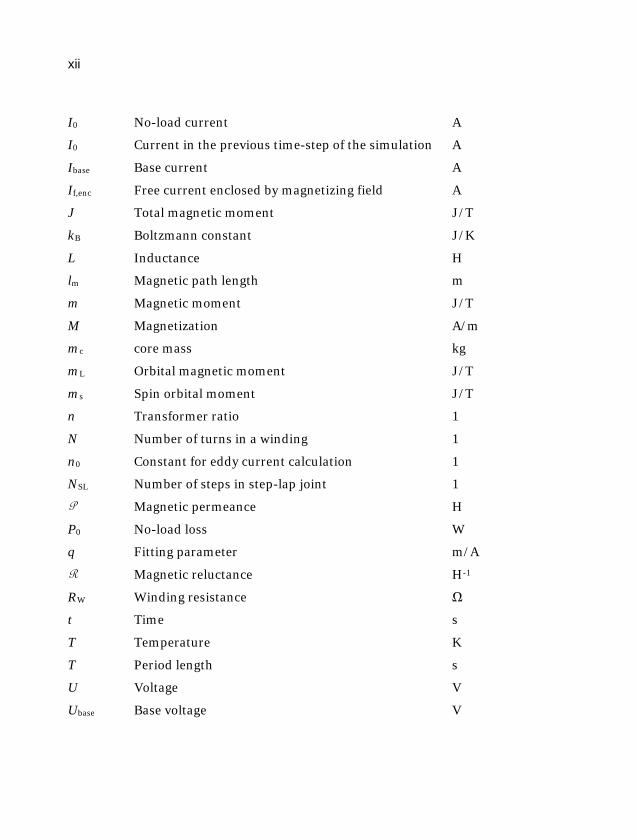
xii
I0 No-load current A
I0 Current in the previous time-step of the simulation A
Ibase Base current A
If,enc Free current enclosed by magnetizing field A
J Total magnetic moment J/T
kB Boltzmann constant J/K
L Inductance H
lm Magnetic path length m
m Magnetic moment J/T
M Magnetization A/m
mc core mass kg
mL Orbital magnetic moment J/T
ms Spin orbital moment J/T
n Transformer ratio 1
N Number of turns in a winding 1
n0 Constant for eddy current calculation 1
NSL Number of steps in step-lap joint 1
P Magnetic permeance H
P0 No-load loss W
q Fitting parameter m/A
R Magnetic reluctance H-1
RW Winding resistance Ω
t Time s
T Temperature K
T Period length s
U Voltage V
Ubase Base voltage V
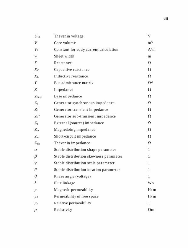
xiii
UTh Thévenin voltage V
V Core volume m3
V0 Constant for eddy current calculation A/m
w Sheet width m
X Reactance Ω
XC Capacitive reactance Ω
XL Inductive reactance Ω
Y Bus admittance matrix Ω-1
Z Impedance Ω
Zbase Base impedance Ω
Zd Generator synchronous impedance Ω
Zd’ Generator transient impedance Ω
Zd” Generator sub-transient impedance Ω
ZE External (source) impedance Ω
Zm Magnetizing impedance Ω
Zsc Short-circuit impedance Ω
ZTh Thévenin impedance Ω
α Stable distribution shape parameter 1
β Stable distribution skewness parameter 1
γ Stable distribution scale parameter 1
δ Stable distribution location parameter 1
θ Phase angle (voltage) 1
λ Flux linkage Wb
µ Magnetic permeability H/m
µ0 Permeability of free space H/m
µr Relative permeability 1
ρ Resistivity Ωm

xiv
ρc Core density kg/m3
φ Phase angle (current) 1
Φ Magnetic flux Wb
ω Angular frequency s-1
1 Introduction
1.1 Background Power transformers have been a key technology for power distribution ever since alternating current won the “war of currents” in the early 1890’s. In the modern grid, power transmission without transformers is unthinkable. However, the dependence on transformers is also a vulnerability. If a large power transformer fails, a large amount of generation may be lost. Replacing a large power transformer costs several million dollars [1], but this pales in comparison to the loss of revenue resulting from a transformer failure. The retail price [2] of the electricity delivered through a large power transformer is several tens of thousands of dollars per hour. Considering that ordering and manufacturing a replacement unit can take more than a year [1], it is easy see the importance of monitoring and maintaining a transformer fleet in order to prevent failures.
In 2011, an internal project was initiated within ABB, tasked with reviewing the available methods for transformer core diagnostics. Transformer cores are generally quite stable and are involved in only a small part of transformer failures. Core failures do happen, however, caused either directly by the core itself or following an electrical or mechanical fault in the rest of the transformer. When they do occur, core faults are usually catastrophic, with temperatures reaching high enough to melt parts of the core. There have also been cases where discoloration or rust has been found on the cores of older transformers following disassembly or during repair. It is therefore reasonable to assume that there are a number of latent core faults in transformers in operation that have not yet developed to the point that they are noticed without opening the tank.
For this reason, it would be desirable to have a method for diagnosing transformer cores, both with the objective of preventing failures, but also with the objective of determining how widespread the problem really is and if something should be done to repair transformers that are still operational, but that are not operating optimally.

2 | Chapter 1 Introduction
The review conducted within that project found several methods for core diagnostics [3]: interlaminar resistance measurement, insulation resistance measurement, thermoscopy (with optic fibers, thermocouples, or with infrared cameras), vibration (noise) measurement [4], frequency response analysis (FRA), and no-load loss measurement [5]. These are all well-known methods, and they are used for routine testing of transformers. Indeed, some of these methods are even required by IEC and IEEE standards. However, the first three methods are designed for testing during production and not on the finished transformer. They are therefore not appropriate for this purpose. Thermoscopy either requires temperature sensors to be installed during manufacturing of the transformer, or it is restricted to measuring the temperature distribution on the outer surface of the tank. This method is therefore also inappropriate for core diagnostics.
Vibration measurements can potentially give a lot of information, particularly about mechanical problems, such as loose clamping. The measurements are, however, notoriously difficult to perform and to interpret. Noise is generated in a transformer both from magnetostriction and from electromagnetic forces. The vibration is then distorted by the mechanical properties of the core and damped by the enclosing oil and tank. So while vibration measurements are promising for core diagnostics, they have too many degrees of freedom, and were considered far too complicated to be pursued.
FRA also shows some promise. It is frequently used for winding diagnostics, and proponents claim that it can also be used for core diagnostics by studying the lower end of the frequency spectrum. The disadvantages of FRA are that the results can be hard to interpret, particularly for the lower end of the spectrum, and that it does not magnetize the core. Since FRA is performed at low voltage, the magnetization of the core changes only a little. This makes the method sensitive to remanent magnetization, and special equipment is required just to get the core to a state where it can be measured.

1.1 Background | 3
The no-load losses are a good indicator of the condition of the core, and major problems with the core will invariably show up in the losses, but it is a rather blunt tool, and gives very little apart from a first indication that something is seriously wrong with the core. There is, however, more detailed data recorded as part of the measurement in the form of the no-load current, and it is this that has been built upon to form this thesis.
During the preliminary studies, it was recognized that a transformer in no-load operation is in principle a machine for measuring the magnetic properties of the core steel, similar to an Epstein frame or single-sheet tester, only much larger. In smaller test equipment, impedances in the measurement circuit can distort the flux wave-shape. Special techniques must then be employed to compensate for these impedances and achieve the desired wave shape. In a large power transformer, however, the magnetizing impedance of the core is dominant. It is therefore easy to measure the magnetic properties of a large power transformer, and it can be done with high accuracy.
Some small-scale tests were performed on table-top model transformers in order to test the diagnostic qualities of the no-load current. These tests confirmed that the no-load current gives much the same information as the no-load losses do, but with better resolution. The no-load loss is a time-averaged value, but the no-load current can be resolved in time and thus give more information and a higher signal-to-noise ratio. These small-scale tests also showed that different kinds of core faults gave different responses in the no-load current and it was therefore possible not just to detect, but also to diagnose the faults.
Since the measurement procedure of the no-load current measurement is identical to that of the no-load loss measurement, which is performed as a routine test, measurements could easily be made even on large power transformers. These measurements gave promising results, with good agreement both between transformers, and with material property measurements.

4 | Chapter 1 Introduction
However, these first measurements were performed on single-phase transformers. When proceeding to three-phase units, the results were suddenly more difficult to interpret. Studies performed on a small distribution transformer (Figure 1) made it clear that the underlying principles remained the same as for single-phase units, but that the interplay between the three phases introduced an additional complexity.
Figure 1: Some small-scale tests were performed on a 100 kVA distribution transformer. Due to concerns about the flammability of the oil-filled transformer, the tests were conducted outdoors, in a tent. The tests were discontinued after the tent was destroyed in a storm during the Christmas of 2011.
The problem was now too large to be treated within the project, and it was decided to expand it into a Ph.D. project. The goal of this Ph.D. project was to further investigate the possibility of using the no-load current as a tool for diagnosing large power transformers either in a factory or in the field, and if

1.2 Aim and scientific contribution | 5
possible, without interrupting operation. A secondary objective was to explain, in detail, the no-load properties of a transformer. This would help transformer designers to improve their designs, and would also help address some of the questions and concerns that often arise during testing. Almost every large power transformer is unique. It can therefore be difficult, both for manufacturers and for users, to determine whether a specific behavior is normal or a cause for concern.
1.2 Aim and scientific contribution The aim of the research project is best summarized by the working title: “The magnetizing current as a tool for on-line transformer core diagnostics”. When the project was initiated, there was no satisfactory way of diagnosing a transformer core. The primary objective was therefore to develop a reliable and non-invasive diagnostic method. If this could be done, the secondary objective was to make it applicable on-line, i.e. without removing the transformer from service.
In order to achieve this, research had to be performed in several related areas. The main scientific contributions of the project are:
• Demonstrating that changes in the core can be detected by studying the no-load currents. This enables diagnostics for any transformer as long as there is a similar unit to compare to.
• Showing that the no-load currents of large power transformers can be measured with high accuracy.
• Developing techniques for comparing the no-load behavior of transformers. Using these techniques, the measured no-load currents depend solely on the magnetic properties of the core. Thus, diagnostics can be performed by comparing two transformers, even if the transformers are not identical.

6 | Chapter 1 Introduction
• Demonstrating a method for performing diagnostics on three-phase transformers by comparing the phases to each other. Thus, diagnostics can be performed even if there is no other transformer to compare to.
• Optimizing a simulation method for studying the no-load behavior of power transformers. The simulations are also validated through comparison to experimental results. This makes it possible to evaluate the impact of faults that are too difficult or costly to test experimentally.
• Developing a curve-fitting method for the major hysteresis loop of grain-oriented electrical steel.

1.3 Previous publications | 7
1.3 Previous publications Some of the methods and results on which this thesis is based have been presented in previous work. The thesis is, in most cases, more exhaustive on these topics, and presents more recent data. The previous publications are, however, often more focused on specific studies, and may be more detailed. A list of publications is therefore presented here for reference purposes.
The licentiate thesis, On methods of measuring magnetic properties of power [6] demonstrates the diagnostic principle and some early results of the project. It also includes more detailed descriptions of some of the early experiments and measurements.
The article Magnetizing Current Measurements on Large Scale Power Transformers [7] describes the techniques used when measuring no-load currents on large power transformers.
The article An application of the time-step topological model for three-phase transformer no-load current calculation considering hysteresis [8] demonstrates the simulation method on a three-phase transformer.
Additionally, the conference contributions A semi-empirical approximation of static hysteresis for high flux densities in highly grain-oriented silicon iron [9] and Power transformer core diagnostics using the no-load current [10] have been presented. The former contribution proposed an expression for approximating the static major loop. At the time of writing, it is undergoing review for publication in Journal of Physics: Conference Series. The latter contribution described an experimental verification of the diagnostic method.
In all these works, the author of this doctoral thesis was the main contributor.

8 | Chapter 1 Introduction
1.4 Thesis outline The first chapter of this thesis describes the background of the project and how it came to be. Chapter 2 then provides a brief introduction to magnetic materials and to power transformers.
The test objects and the equipment used in the thesis are described in chapter 3. The chapter also describes the measurement method. Chapter 0 shows the results from measurements both on large power transformers and on smaller units. This establishes the differences and similarities between transformers of different sizes and designs. This is intended to show that, if the correct techniques are employed, power transformers yield consistent measurement results.
Chapter 5 describes a simulation method, and how it can be refined to give highly accurate results for no-load conditions. The chapter also shows comparisons between measurements and simulations. Additionally, the chapter shows how different simplifications affect the simulation results.
These simulations also help explain some of the phenomena that occur specifically in large power transformers. These phenomena are often quite straightforward. However, since measurements on large power transformers are scarce, they have not been well documented previously. The consequences of these phenomena may therefore not be apparent. For this reason, Chapter 6 describes some of the phenomena that affect the no-load currents
Finally, the stated aim of the project is to develop a method for transformer core diagnostics. Chapter 7 describes this diagnostic principle, and gives examples from simulations and experiments. The chapter also describes the impact of different types of core defects. In order to develop the method into a fully functional tool, some further work is required. This further work, along with some possible spin-offs from the project, is discussed in chapter 8. Chapter 9 then concludes the thesis with a summary of the research outcomes.
2 Magnetism and power transformers
The core of a large power transformer accounts for almost half of the total mass of the transformer and yet it is not given as much attention as the windings, bushings, tap-changers, or other components that make up the transformer. One could argue that this is fair: the core has only seen gradual improvements since the first transformers, it accounts for only a small part of the losses, and it rarely breaks. Nevertheless, the core is the heart of the transformer, and the transformer cannot perform to its full potential if the core is not in perfect condition. The core is also far more complex than it might at first appear. The magnetic properties are highly non-linear and anisotropic, and are intimately connected to the electrical properties of the rest of the electrical circuit.
This combination of complexity and importance was the reason for initiating this thesis work. In order to manufacture and maintain high-quality power transformers, and to maximize efficiency and reliability, there must be a way to predict the behavior of the core, and to detect any defects. There are presently few satisfying methods for diagnosing transformer cores.
2.1 Notes on terminology and conventions
2.1.1 The magnetic fields In magnetism, there are three commonly used field quantities: the magnetization M, the flux density B, and the magnetizing field (or H-field), H. These quantities are related via the vacuum permeability 𝜇𝜇0 ≡ 4𝜋𝜋10−7 H/m, through the expression
𝑩𝑩 = 𝜇𝜇0(𝑯𝑯 + 𝑴𝑴). (1) This expression describes magnetism on a fundamental level, but in engineering applications it can be impractical. Measuring the magnetization can be done either by measuring the force on the sample in an external field, or by direct imaging using e.g. the magneto-optic Kerr effect, electron microscopy, or magnetic force microscopy [11]–[13]. All of these methods require direct access to the sample and a small sample size. They are not

10 | Chapter 2 Magnetism and power transformers
useful for large transformer cores. Therefore, it is common to introduce a relative permeability 𝜇𝜇r and use the simpler expression
𝑩𝑩 = 𝜇𝜇0𝜇𝜇r𝑯𝑯. (2) Both B and H can be measured, or at least approximated, from outside the transformer. Faraday’s and Ampère’s1 laws give, respectively,
�𝜕𝜕𝑩𝑩𝜕𝜕𝜕𝜕
∙ 𝑑𝑑𝑨𝑨𝑆𝑆
= −� 𝑬𝑬 ∙ 𝑑𝑑𝒍𝒍𝜕𝜕𝑆𝑆
(3)
� 𝑯𝑯 ∙ 𝑑𝑑𝒍𝒍𝐾𝐾
= 𝐼𝐼f,enc (4)
As long as the flux density is constant across the core cross-section S, the flux density can be calculated from the turn voltage. Similarly, as long as the magnetizing field is constant along the length of the core K, it can be calculated from the enclosed current, If,enc , i.e. from the number of turns N and the magnetizing current 𝐼𝐼0 = 𝐼𝐼𝑓𝑓,𝑒𝑒𝑒𝑒𝑒𝑒/𝑁𝑁. Equations (3) and (4) can then be simplified to
𝐵𝐵 =1𝑁𝑁𝑁𝑁
�𝑈𝑈𝑑𝑑𝜕𝜕, (5)
𝐻𝐻 =𝑁𝑁𝐼𝐼0𝑙𝑙m
. (6)
Thus, the fields are given by the applied voltage U, the magnetizing (or no-load) current 𝐼𝐼0, the cross-sectional area A, and magnetic length 𝑙𝑙m of the core, and the number of turns. All of these quantities can easily be measured or found from design data2.
The validity of these approximations will be discussed further in chapters 3.1 and0, but it can be noted that in order for them to hold, the fields must be uniformly distributed and parallel. For this reason, the fields will be given as
1 The displacement current, which is included in the more general Maxwell-Ampère equation, is neglected here. 2 Though the values can be slightly ambiguous, particularly for 𝑙𝑙m. This will be discussed further in chapter 4.1.

2.2 Magnetization of core steels | 11
scalars, rather than vectors, and B = |B||| and H = |H||| denote the components that are parallel to the core.
However, it must be pointed out that the theoretical treatment of magnetism is based on the fields in (1). When B(M) and B(H) are used interchangeably in this thesis, this should be seen as an engineering approximation, not as physical fact.
2.1.2 Magnetizing current and no-load current The term magnetizing current is often used to mean the current drawn by a transformer that is being magnetized but not loaded. However, this current often contains other components than just the magnetization of the core steel. The more correct term no-load current will therefore be used instead, and magnetizing current will be reserved for the current component that goes into magnetizing the core. The difference between no-load current and magnetizing current will be discussed further in Chapters 6.1 and 6.5.
2.2 Magnetization of core steels
2.2.1 Ferromagnetism and static hysteresis When magnetized, transformer cores exhibit several particular properties such as high magnetic permeability, non-linearity, and hysteresis. These properties are results of the steel that makes up the core being a ferromagnetic material. In order to understand the magnetic behavior of a transformer core, it is therefore necessary to take a closer look at the underlying atomic theory of magnetism.
In an atom, electrically charged electrons orbit the nucleus. This represents a current flowing in a closed loop around the nucleus, and according to Ampère’s law, this gives rise to a magnetic field perpendicular to the plane of rotation (see Figure 2a). Additionally, the electrons themselves also contribute to the magnetic field through a fundamental property known as

12 | Chapter 2 Magnetism and power transformers
electron spin3 [14]. The total magnetic moment of the atom is then the sum of all these spin and orbital contributions.
Figure 2: a) A simplified atomic model of an electron orbiting a nucleus, thus giving rise to an orbital magnetic moment mL. The electron itself also has a spin magnetic moment ms that contributes to the total magnetic moment. b) The magnetic moments of the atoms in a ferromagnetic crystal tend to align in the same direction, even absent an external field.
In many atoms, the magnetic moments are oriented such that they cancel out, giving the atom a zero total magnetic moment. These types of materials are called diamagnetic [15]. Diamagnetic materials react very weakly to an external magnetic field. As a consequence, diamagnetism is of no interest in this thesis.
If a material with a non-zero total magnetic moment, on the other hand, is subjected to an external field, the moments align with the applied field and also enhance it. That is to say that the total field in the material becomes the
3 The term spin is somewhat misleading as the electron is nowadays considered to be point-like. The explanation that the magnetic moment is caused by a charge distribution orbiting around its own axis is therefore incorrect. The term spin remains for historical reasons.

2.2 Magnetization of core steels | 13
applied field plus the contribution from the magnetic moments that have aligned with the field. When the applied field is removed, the behavior of the material depends on the strength of the interaction between magnetic moments. If the interaction is weak, random thermal agitation is sufficient to make the material lose its ordering. The magnetic moments align randomly, and the total magnetization of the sample returns to zero. These materials are called paramagnetic. However, if the interaction is strong enough, they will affect each other enough to stay aligned (Figure 2b). Thus, the material remains magnetized even when the applied field is removed. This interaction is called the exchange interaction, and these materials are ferromagnetic.
The exchange interaction is also responsible for hysteresis in ferromagnets. In order to demagnetize a ferromagnet, it is not sufficient to just turn off the magnetizing field; it is necessary to apply a magnetizing field in the opposite direction. This means that every time the applied field changes directions (as happens in a transformer core twice every ac cycle), some energy is required just to change the direction of the magnetization. This is, of course, undesirable, and transformer core steel is designed to have as little hysteresis as possible. Hysteresis is, however, intrinsic to ferromagnets and can not be fully eliminated.
Since hysteresis is related to changes in the magnetization, it depends on the state before the change occurs. Therefore, the size and shape of the hysteresis curve depends on the reversal point, i.e. on the values of B and H (or, strictly speaking, M and B). One well-defined reversal point is at full saturation of the material, and the major hysteresis loop, which goes between positive and negative saturation, is therefore often used as a reference (see Figure 3). However, because of the high applied field required to reach saturation, it is more common for measurements to show minor loops. Of the minor loops, first-order reversal curves (FORC), i.e. minor hysteresis curves with reversal point somewhere on the major loop, are of particular interest.

14 | Chapter 2 Magnetism and power transformers
Figure 3: Major loop (with reversal at 2.03 T) and a minor loop (reversal at 1.7 T) for a transformer steel. Since the reversal point of the minor loop lies approximately on the major loop, it can be considered a FORC. Note that the major loop has been truncated at 100 A/m. The actual magnetizing field at saturation is approximately 10 kA/m.
Paramagnetic and ferromagnetic materials have several common characteristics. In fact, ferromagnets become paramagnetic at high temperatures4, when the thermal agitation becomes stronger. One of the main similarities between the two types is that both are non-linear. At low applied fields, a small increase of the applied field is enough to align several moments, thus leading to a large increase in the total field. At higher applied fields, only a few moments remain unaligned, and an increase of the applied field leads to only a small increase of the total field. Finally, when all the magnetic moments have aligned, increasing the applied field further does
4 The temperature at which the material transitions to being paramagnetic is called the Curie temperature. In electrical steels such as those used in transformers, the Curie temperature is 750 °C -800 °C [16]

2.2 Magnetization of core steels | 15
nothing to the material. The magnet has saturated, and the total field is equal to the saturation field, i.e. the field from the magnetic moments, plus the applied field.
The behavior of the magnetic moments is governed by statistical mechanics, and it is pointless to talk about individual moments. In theory, however, it is possible to predict statistically the distribution of magnetic moments in a ferromagnet by finding the configuration that gives the lowest total energy [17]–[19]. The main contributions to the total energy are the Zeeman energy EZ, the exchange energy Eex, and the anisotropy energy Eai:
𝐸𝐸tot = 𝐸𝐸Z + 𝐸𝐸ex + 𝐸𝐸ai. (7)
The Zeeman energy is the energy due to the applied field, and is the only contribution that can be easily calculated. With applied field 𝑩𝑩a and magnetic moment m,
𝐸𝐸𝑍𝑍 = 𝒎𝒎 ∙ 𝑩𝑩a. (8) The exchange energy is the energy associated with the exchange interaction between all magnetic moments. Most ferromagnets are crystalline5, and as a result, the distance, and therefore the strength of the exchange interaction, between neighboring moments is direction-dependent. This leads to anisotropy; i.e. it is easier to magnetize the material in certain directions than in other. In modern transformer steels, there are usually three “easy” directions: one in the direction in which the steel is intended to be magnetized (the rolling direction), and two more directed 45° out of the plane.
In addition to the exchange interaction being anisotropic, there are additional anisotropies that contribute to the anisotropy energy [20]. For transformer core steel, the most important contributions are shape anisotropy, surface anisotropy, and magnetoelastic anisotropy. The first two have to do with how the magnetic material interacts with its surrounding (Figure 4a). A magnetic moment at the interface to a different material 5 The exceptions are so-called amorphous ferromagnetic materials.

16 | Chapter 2 Magnetism and power transformers
experiences very different conditions from the two sides. Magnetoelastic anisotropy occurs when the material is subjected to a mechanical stress. Somewhat simplified: if the material is compressed, the magnetic moments come closer to each other, thus affecting the strength of the exchange interaction in that direction.
In practice, these interactions are so complex that analytically minimizing the total energy in (7) is impossible except in very simple geometries or in small samples [21]. Nevertheless, one consequence that can be directly observed is the formation of magnetic domains [22]. In large crystals, it is energetically favorable for the material to divide up into domains in which all the magnetic moments are aligned parallel to each other (Figure 4b-c)6. In this way, a majority of the magnetic moments can be aligned in one of the easy axes, thus minimizing the stored energy. At the same time, the relative sizes of the domains can be such that the total magnetization of the sample is close to the applied field, thus minimizing the Zeeman energy. However, having two adjacent magnetic moments with opposite alignments carries a high energy cost. To reduce this energy, there is a boundary region, a domain wall, between adjacent domains. In the domain wall, the magnetization direction changes gradually, over a distance of a few hundred atoms.
6 The domain structures shown here are simplified. In reality, the minimization of energy usually requires domains in other directions as well [23].

2.2 Magnetization of core steels | 17
Figure 4: a) Since the permeability of free space is much lower than that of the steel, the anisotropy energy of a moment that is parallel to the boundary (bottom image) is much lower than that of a moment at an angle to the boundary (top image). This tends to make the magnetic moments align along the steel sheet. b) Formation of magnetic domains in easy magnetization direction of the steel reduces the total magnetic energy. However, the magnetic flux must still form closed loops. If the flux closes in air, this leads to a high magnetic energy. c) If the flux instead closes through formation of 90° domains, the total energy can be reduced.
Changes of magnetization in a multi-domain ferromagnet mainly take place through domain multiplication, where new domains are formed out of the existing ones, or through domain wall movement. Through these processes, the total magnetization of the sample can change without requiring the domains to change their alignments away from the easy directions. Such domain rotation carries a high energy cost and usually occurs only close to saturation when there is no other option.

18 | Chapter 2 Magnetism and power transformers
Figure 5: The magnetization of the steel changes mainly through domain wall movement. At low applied field (a), the domains are approximately the same size, giving a low total field. As the applied field increases (b), the domains that are aligned along the applied field expand, while the domains opposing the applied field shrink.
2.2.2 Dynamic hysteresis The hysteresis described in the precious section is the so-called static hysteresis, which is independent of the rate of change of the magnetization. If the magnetization changes more quickly, this induces a voltage in the core in the same way as in a transformer winding. This leads to eddy currents in the core, and thus to increased losses. In the B-H plane, an increase in losses manifests as a widening of the hysteresis curve, and this contribution can therefore be seen as a hysteresis contribution.
The total dynamic hysteresis, as it is measured in transformers, is therefore a sum of static hysteresis and eddy losses. Figure 6 shows a number of dynamic hysteresis curves measured with different amplitudes of sinusoidal flux density. With fixed frequency, changing the peak flux density leads to a change of the rate of magnetization, and thus also the amount of eddy currents.

2.2 Magnetization of core steels | 19
Figure 6: Dynamic hysteresis curves at 50 Hz. The dynamic losses depend on the peak flux density, and the dynamic hysteresis curves are therefore different for each of the five different peak flux densities shown in the figure.
Eddy currents can be divided into two types: classical eddy currents and excess eddy currents. The classical eddy currents, and the corresponding field Hcl, can be calculated using classical electromagnetic theory [24], [25]. There are several ways of doing this, and the exact expression for Hcl depends on the amount of detail and on what the solution should be used for, but here it is sufficient to consider the low-frequency solution. If the rate of change is (i.e. frequency) is high, the eddy current field reduces the total field in the center of the material. This eddy current shielding leads to an uneven flux distribution and a more complicated eddy current behavior. However, if the rate of change is low enough, as is assumed here, the applied field penetrates fully and distributes evenly throughout the whole sample. In that case,
𝐻𝐻cl =𝑑𝑑2
12𝜌𝜌𝑑𝑑𝐵𝐵𝑑𝑑𝜕𝜕
, (9)
where d is the thickness of the steel, and 𝜌𝜌 is the resistivity.

20 | Chapter 2 Magnetism and power transformers
The measured losses and dynamic hysteresis of transformer steels is, however, significantly higher than what can be explained by classical eddy currents alone. This difference is called excess loss and is caused by the motion of the domain walls. When domain walls move, they do so between different local energy minima. This means that a domain wall might remain stationary and then suddenly jump to a new state when the applied field becomes high enough. These jumps can be caused by the domain wall becoming pinned behind a defect in the steel, or having to pass a state with a higher anisotropy [26].
The excess eddy current field is very difficult to predict exactly, but it can be approximated using the phenomenological constants7 V0 (with unit Am-1) and n0 (unit 1) [24]. These constants characterize how often the domain walls jump, and the average energy, though their exact physical interpretation is more complicated and will not be discussed here.
The expression that will be used here for the excess eddy current field is
𝐻𝐻ee =𝑛𝑛0𝑉𝑉0
2��1 +
4𝐺𝐺𝐺𝐺𝑑𝑑𝜌𝜌𝑛𝑛02𝑉𝑉0
𝑑𝑑𝑑𝑑𝑑𝑑𝜕𝜕
− 1�, (10)
where G is a geometric factor. For a steel sheet of the type used in transformers,
𝐺𝐺 = 4/𝜋𝜋3 �1𝑘𝑘3
𝑘𝑘 𝑜𝑜𝑜𝑜𝑜𝑜
≈ 0.1356. (11)
It is interesting to note that the excess eddy current field depends on the sheet width w. This is somewhat surprising, since sheet width is not usually considered when measuring losses [27]. However, since V0 and n0 are also functions of the lamination dimensions, the dependence is very weak.
7 V0 and n0 should depend on the magnetization state, but they will be considered constant here.

2.2 Magnetization of core steels | 21
2.2.3 Anatomy of the hysteresis curve Finally, it is useful to define some terminology for the hysteresis curve (Figure 7). As described earlier, the steel retains some magnetization even when the applied field is removed. If H is seen as the applied field, this means that as the field is turned off, the flux density will go to some non-zero remanent flux density, Br. Conversely, if B is seen as the applied field, the magnetizing field will go to the coercivity, Hc. In practice, it is uncommon for B to be directly controlled. Therefore, Hc is mostly relevant as a measure of the current required to bring the flux density to zero. Br, on the other hand, is the amount of flux that will remain in the core if the supply is suddenly switched off.
Figure 7: Terminology for different parts of the hysteresis curve.
The magnitude of the remanence and of the coercivity depends on the reversal point (as can be seen in Figure 3), and on the rate at which the applied field is changed.

22 | Chapter 2 Magnetism and power transformers
The knee is where the steel starts to saturate, and it is the point with the highest permeability 𝜇𝜇 = 𝐵𝐵 𝐻𝐻⁄ . This is a useful property for giving an exact definition of the knee, but it is debatable whether the concept of permeability is at all relevant in in hysteretic materials. At least, the definition 𝜇𝜇 = 𝐵𝐵 𝐻𝐻⁄ leads to a permeability that can be both negative (in the second and fourth quadrants of Figure 7) and infinite (at the remanence point).
2.3 Power transformers This section gives a brief introduction to how transformers, and in particular large power transformers, are designed and constructed.
2.3.1 Factors affecting transformer design Physical size is one of the major limitations when designing transformers. A transformer must be small and light enough to transport from the factory to the power station. If it is too heavy, it will be impossible to transport by road or railroad, and there will be no cranes capable of moving it onto a ship. If it is too large, it will be impossible to transport through tunnels or under bridges, and buildings and structures close to the road may need to be removed or demolished. Additionally, larger units, requiring more raw materials, tend to be more expensive. For these reasons, power transformers tend to be designed to be as small as possible.
In addition, the specifications naturally affect the design of a transformer. Apart from the rating and the choice of accessories, there are a few other factors that determine how a transformer is designed. For the core, the most important are the loss evaluation, the noise level requirements, and the overvoltage capability requirements.
A transformer is an investment that can be expected to remain in operation several decades [28]. During this time, the cost of operating the transformer can accumulate and become higher than the purchasing cost. Transformers are therefore usually sold with consideration taken for the total ownership cost (TOC). The TOC includes the purchasing price, capitalization of losses, and in some cases service agreements.

2.3 Power transformers | 23
The capitalization of losses is based on how much money the customer expects to lose from losses, i.e. how much electricity that is lost in the transformer could otherwise have been sold for [29]. This is expressed as a loss evaluation in dollars (or euro) per kilowatt of losses, and depends on the projected electricity price and on how long the transformer is expected to operate. The loss evaluation is different for load losses, which are dependent on the load, and for no-load losses, which are always present when the transformer is connected to the grid. Thus, unless the transformer is expected to constantly operate at 100 % of its rated power, the no-load loss evaluation will always be higher than the load loss evaluation.
Most substations, particularly in residential or recreational areas, have to follow sound level restrictions. Therefore, a limit on the maximum sound level of a transformer is usually included in the specification. Noise is generated in transformers from a variety of magnetic and electromagnetic forces, but core noise is one of the main contributions. Core noise is mainly caused by magnetostriction and increases with increasing flux density. In order to meet a strict noise requirement, it might therefore be necessary to limit the flux density of the core.
A final limiting factor on the core dimensions is the overvoltage capability. Most transformers must be capable of operating for short periods of time above rated voltage. The exact level of overvoltage varies, but 10 % is quite common. This places an upper limit on the flux density in the core, since the core should not saturate even under those 10 % higher voltage.
All these factors have to be considered when designing a transformer core, and design criteria for other parts of the transformer often influence the core design as well. It is therefore difficult to make any sweeping statements about how transformer cores are constructed. There are, however, some common characteristics. For instance, cores are usually designed with rated flux densities around 1.7 T to 1.75 T. In cases where the noise restrictions or the overvoltage requirements are stricter, this is lower.

24 | Chapter 2 Magnetism and power transformers
A final note on the construction of large power transformers is that much of the process is done by hand. The reason for this is mainly that large power transformers are highly customized. Every large power is usually constructed for use in a specific power plant or substation. Even though voltage levels are usually standardized, other parameters, such as rated power, short circuit impedance, loss evaluation, or noise requirements, often vary. Therefore, almost every transformer is unique, making manual labor a more competitive option than an automated process.
2.3.2 Transformer windings and vector groups The windings are an important part of a transformer, but for the purposes of this thesis, they are mainly a way of magnetizing the core, and their exact construction will not be given any particular focus. The only relevant quantities are the number of turns and the physical dimensions, since these define how the flux is distributed in the core and the surrounding air.
Similarly, the vector groups of the windings (i.e. how they are connected) are only of interest insofar as they affect the magnetization of the core. This, combined with the fact that large power transformers usually do not have exotic vector groups, means that in all the transformers described in this thesis, there are only three vector groups (Figure 8). These are grounded wye (YN), ungrounded wye (Y), and delta (D). The vector groups are often further subdivided depending on the phase shift that they cause between the windings, but again, that is not relevant to the magnetization, and will be ignored. It is, however, worth pointing out that the high voltage (HV) winding will most often be Y- or YN-connected, since this gives a lower voltage over the winding. Almost all large power transformers also have a delta winding, either as one of the main windings, or as a tertiary winding whose sole purpose is to provide a delta winding.

2.3 Power transformers | 25
Figure 8: Winding diagrams of the three vector groups used in the thesis.
Since the winding arrangement is not important for the no-load loss, the winding from which the transformer is magnetized during testing is not always the same as the winding from which it will be magnetized in service. For this reason, the term primary will be used to refer to the winding from which the transformer is currently magnetized, regardless of how the transformer is designed to be operated. If there is any risk of ambiguity, the voltage levels will be given instead, i.e. HV (high voltage), LV (low voltage) or tertiary.
Following the prevalent standards, properties relating to the different windings are written separated by a slash and in the order HV/LV/tertiary/other windings.
2.3.3 Transformer rating and the per-unit notation The transformer is rated with respect to voltage, power, and frequency. The voltage and power ratings are given for each winding separately.
The rated voltage is given for each winding, and always as the phase-to-phase voltage, regardless of how the winding is connected or whether the transformer is single-phase or three-phase.
The rated power of a transformer is given in terms of total throughput power, but the definition varies slightly between standards. The IEC [5] defines rated power as the power input into the transformer, while the IEEE

26 | Chapter 2 Magnetism and power transformers
[30] defines it as the power output from the transformer. The rated power according to the IEEE standard is therefore lower by an amount equal to the transformer losses. This difference is usually approximately one percent. This thesis focuses mainly on large power transformers, i.e. transformers with rated power above 100 MVA for three-phase units, or 33.3 MVA for single-phase units [31].
The rated frequency is always equal to the power frequency and depends only on where the transformer is to be installed. All the transformers used in this thesis are rated at either 60 Hz, for most of the Americas, or 50 Hz, for the rest of the world. Additionally, some specialized systems may operate at other frequencies. One example is the Swedish railway system, which runs at 16.7 Hz. However, these systems do not use large power transformers, and are not relevant for this thesis, except as sources of interference.
Finally, the short-circuit impedance can in some sense be considered a rating. Though not explicitly listed as a rated quantity in IEC 60076-1, the short-circuit impedance is invariably given on the rating plate of a transformer. The short-circuit impedance of a pair of windings (e.g. HV/LV) is defined as the equivalent series impedance of one winding when the other winding is short-circuited at the terminals. Since the short-circuit resistance is negligible, the short-circuit impedance
𝑍𝑍𝑠𝑠𝑒𝑒 ≈ j𝜔𝜔𝐿𝐿12, (12) where ω is the angular frequency, and 𝐿𝐿12 is the leakage inductance between the two windings.

2.3 Power transformers | 27
Since the voltages, currents, etc. vary so much, even between windings in a single transformer unit, it can be easier to consider them instead as percentages of the some base quantities [32]. For transformers8, the rated power is used as the base power, Sbase, and the rated voltage as the base voltage, Ubase. From this, the base current, Ibase, and base impedance, Zbase, are calculated:
𝐼𝐼base =𝑆𝑆base
√3𝑈𝑈base, (13)
𝑍𝑍base =𝑈𝑈base2
𝑆𝑆base. (14)
Now, any current, voltage, power or impedance9 can be expressed as a fraction of these base quantities. This is usually done in either percent or per unit.
For example, consider a 500 MVA 400 kV/135 kV transformer with a short circuit impedance of 48 Ω seen from the HV side. The base impedance of this unit, on a 500 MVA, 400 kV base, is Zbase = 320 Ω, and the per-unit short circuit impedance is then 48/320 = 0.15 p.u. The same short-circuit impedance, seen from the LV side is 48·(135/400)2 ≈ 5.5 Ω, but this is also 5.5/(1352/500) = 0.15 p.u.
The advantage of this method is that any quantity expressed as a per-unit value will be the same on both the primary and the secondary of the transformer, even if the actual numerical value varies by several orders of magnitude.
8 In a power grid, other values may be used depending on which point in the grid should be used as the reference and what the aim of the calculation is. 9 When expressed in per unit, the short-circuit impedance is equal to the voltage drop over the transformer at full rated load. For this reason, in Sweden, it is often denoted Uk (k for kortslutning), even though it is not a voltage.

28 | Chapter 2 Magnetism and power transformers
2.3.3.1 Impedances and Thévenin equivalents Any linear electrical circuit can be simplified to a voltage source behind an impedance. The voltage of this voltage source, known as the Thévenin voltage 𝑈𝑈Th is equal to the open-circuit voltage, and the impedance 𝑍𝑍Th is equal to the short-circuit impedance.
This so-called Thévenin equivalent is often useful for analyzing a system, since it allows large systems to be reduced to just two components: a voltage source and an impedance.
An important caveat is that Thévenin equivalents can only be derived for linear circuits, and many power system components are non-linear to some extent. For example, transformer and generator cores are inherently non-linear, and control equipment such as power electronics or tap changers introduce non-linearities. Nevertheless, the concept of Thévenin equivalents is so convenient that it is often easier to linearize the system than to handle the full, non-linear, system.
For transformers, this means that the short-circuit impedance is only valid for the rated frequency. The frequency dependence of the short-circuit impedance is quite simple, however. The short-circuit impedance depends almost entirely on the leakage inductance between the windings 𝐿𝐿12. Since this is an air inductance, it is constant. For two transformer windings, neglecting end effects, this inductance depends only on the number of turns N1 in the magnetizing winding, the length of the winding l1, and the area between the windings. If the windings have are approximated as concentric solenoids with cross-sections 𝑁𝑁1 and 𝑁𝑁2,
𝐿𝐿12 ≈𝑁𝑁12|𝑁𝑁1 − 𝑁𝑁2|
𝑙𝑙1. (15)

2.3 Power transformers | 29
It is, however, only the leakage inductance that is constant. The magnetizing inductance of the core is definitely not constant, nor linear. It can not be reduced to a Thévenin equivalent10.
As mentioned, generators are also inherently non-linear, and the short-circuit impedance of a generator depends on the time-scale of the phenomenon that is being studied. The short-circuit impedance of a generator is therefore usually divided into three parts. These are the sub-transient, transient and synchronous impedances [33].
The subtransient inductance is the self-inductance of the stator winding. For fast events (less than a period), this is the dominant inductance. It therefore determines the instantaneous voltage drop due to the no-load current of a transformer, and is thus the only relevant generator inductance in this thesis. The subtransient impedance 𝑍𝑍d′′ is usually in the range of 10 % to 30 %.
The transient and synchronous impedances operate on longer time-scales, and are therefore not relevant to the work presented here. They are mentioned only for completeness. Just as the sub-transient inductance is related to the stator flux linkage, these other inductances are also related to flux linkage components in the generator. The synchronous inductance corresponds to the flux linkage of the exciter winding. This generally changes only very slowly, over the course of several seconds. The synchronous impedance 𝑍𝑍𝑜𝑜 is high, several hundred percent. This can be understood intuitively: once the generator loses excitation, the voltage will drop dramatically.
The transient inductance corresponds to the flux linkage that induces currents in the other windings of the generator (primarily in the armature). This has the effect of damping oscillations in the generator. The transient
10 Since the magnetizing current is so much lower than the load current (usually less than one percent) in a power transformer, the non-linearity is often neglected. In that case, it is of course possible to use it in a Thévenin equivalent. This thesis, however, is about the magnetizing current. Consequently, the non-linearity is of the utmost importance.

30 | Chapter 2 Magnetism and power transformers
impedance 𝑍𝑍d′ is usually approximately the same magnitude as the subtransient impedance, or slightly larger. It operates on time scales of a few periods.
2.3.4 Core geometries There are two basic ways of constructing a transformer. Either the winding is placed around the core (core-type), or the core is placed around the winding (shell-type). Shell-type transformers typically use more core steel than core-type transformers, and the construction is therefore less common in large power transformers. As a consequence, the full focus of this thesis is on core-type transformers.
Table 1: Core type designations depending on the number of wound limbs and whether the unit has return limbs. For reference, the table also includes the Swedish abbreviations EY, DY, and TY. Here, Y stands for ytterben.
No return limbs Return limbs
1 wound limb - SR (EY)
2 wound limbs D DR (DY)
3 wound limbs T TR (TY)
4 wound limbs Q QR
The simplest core geometry for a three-phase power transformer is with just three wound limbs. This is known as a three-limb core or T-core (Table 1), and makes up the majority of all large power transformers, and almost all smaller power transformers. For higher rated power, transport height often becomes a problem, and the transformer can then be made lower by reducing the yoke height and instead adding return limbs (see Figure 9). The resulting five-limb core, or TR-core has a higher total mass, but lower height.

2.3 Power transformers | 31
Figure 9: The most common core geometries are the T- and TR-cores for three-phase transformers, and the D-, DR, and SR-cores for single phase cores. In three-phase units, each phase is wound on a single limb11, while in single-phase units, the winding may be split up in order to further reduce the dimensions. If this is done, the windings must be wound and connected in such a way that the flux can close (red arrows).
If the transformer is still too large, it can be split into several smaller units. This is often done with transformers for HVDC (high-voltage direct current) applications as the total transferred power can be several GVA: far too much for a single transformer to handle. This way, one enormous three-phase transformer can be replaced by three (or sometimes six or more) single-phase units.
In addition to making transport easier, this also has the benefit of making repairs and replacements easier. The process of manufacturing and delivering a large power transformer can take years and is associated with large costs, and for this reason, many users want a spare unit that can be installed quickly in the case of a failure. Buying a fourth unit for a bank of
11 There are some exceptions, e.g. some phase-shifting transformers.

32 | Chapter 2 Magnetism and power transformers
three single-phase units is much cheaper than buying a second three-phase unit.
Similar to three-phase transformers, single-phase transformers can also be made with or without return limbs. It is also possible to split the winding onto two limbs in order to further reduce the size. This gives three common single-phase core types: with two wound limbs, either with (DR) or without (D) return limbs, and with a single wound limb plus return limbs (SR). In addition, there are single-phase transformers with three (TR-1)12 or four (QR) wound limbs. These are not shown in the figure, but the geometries can easily be deduced from the smaller units.
2.3.5 Autotransformers
Figure 10: In an autotransformer, the same winding is used for both the primary and secondary.
Another way of reducing the size of a transformer is designing it as so-called autotransformer. An autotransformer has a single winding for both the
12 The core with three wound limbs plus return limbs is the only core geometry that can be used for both single-phase and three-phase transformers. The single-phase transformers are therefore designated here as “TR-1” to avoid confusion.

2.3 Power transformers | 33
primary and the secondary, and is therefore smaller than a full transformer of the same rated power. The drawback of an autotransformer is that it does not provide any electrical insulation between the primary and secondary. Autotransformers are also not suited for high conversion ratios since a high conversion ratio would mean that the part of the winding that is common to both primary and secondary is small, thus negating the advantage of the autotransformers.
2.3.6 Core steel The main purpose of the transformer core is to guide the flux through the windings. In order to fulfill this purpose, the core should have high magnetic permeability and low losses, and be able to sustain a high flux density. It must also have good mechanical properties and be reasonably cheap.
The earliest transformers used solid iron cores to guide the flux through the windings, but this leads to high losses from eddy currents. To solve this, the core is split into thin sheets or laminates, which are coated with an insulating material to increase the resistance between adjacent sheets. The resistivity of the steel is also increased by alloying the iron with silicon.
A few percent of silicon also has the benefit of increasing the saturation magnetization of the steel, which means that the core can be made smaller and still carry the same amount of flux. However, the silicon also makes the steel brittle and difficult to handle. A high silicon content can also make the manufacturing process more difficult [34]. Therefore, the steel used for large power transformers is made with 3 % silicon, but higher silicon contents are used in steel for some smaller transformers.
Steel is crystalline and has a body-centered cubic structure, which gives it a crystal anisotropy. That is to say, the crystal magnetizes easier in some directions (the <100>, <010>, and <001> directions) than in others. In a normal steel sheet, the individual crystals are aligned randomly, but in 1935, Norman Goss patented a method for getting the crystals to align in the rolling direction (the direction in which the steel is intended to be

34 | Chapter 2 Magnetism and power transformers
magnetized) [35]. With this method, the steel forms large crystal grains, all approximately aligned in the same direction.
The alignment can be further improved by applying a stress-coating to the surface of the sheet [36]. This introduces a tensile stress in the rolling direction and thereby increases the shape anisotropy. That is to say that the permeability increases in one of the easy directions while decreasing in the other two. By making sure that the easiest direction is in the rolling direction, this results in a higher-permeability core.
The next improvement came in the sixties with the realization that certain precipitates such as aluminum nitride [37] can be used to promote the grain orientation. These highly grain-oriented steels (called Hi-B by the inventors, Nippon Steel Corporation) have still higher permeability and lower hysteresis losses. However, when the grain size increases, so does the size of the magnetic domains, and this leads to higher excess eddy losses.
To decrease the eddy current losses while still keeping the high permeability, the magnetic domains can be made smaller by scratching or etching the surface of the steel [38]. Using a laser or a needle, disturbances are introduced in the steel where the anisotropy is different than in the rest of the sheet. At these points, 90˚ domains are formed, which allow the 180˚ domains to close (Figure 11). This makes the average domain smaller, and decreases eddy current losses.

2.3 Power transformers | 35
Figure 11: The steel forms crystal grains (a). In these grains, the domains (gray and white in (b) and (c)) mainly align along the rolling direction. Domain refinement (c) introduces 90° domains (blue), where the magnetization is perpendicular to the rolling direction. This reduces the average domain width, reducing excess eddy current losses.
As can be seen from this timeline, the transformer core has remained more or less the same since induction was first discovered by Faraday and Henry, almost two hundred years ago. The development of the core steel has not been characterized by any quantum leaps forward, but rather by continuous small improvements. There are still transformers in service today that were built more than fifty years ago, and there is thus a large variation of transformer steel types. From conventional grain oriented (CGO) steels of the type developed by Goss in the thirties, through the highly grain-oriented (Hi-B) steels of the type developed by Taguchi et al. in the sixties, to the domain refined steels used in modern transformers. Though the progress has been slow and gradual, it has been substantial. A modern, 0.23 mm thick, domain refined steel has less than half the specific losses of a 0.5 mm CGO steel of the type used in transformers from the sixties and seventies.
This thesis treats only grain-oriented steels, but there are several other possible alloys and treatments that are used for electrical steel. Of these, amorphous steel [39] is also mentioned here since it is used in some small power transformers and distribution transformers.

36 | Chapter 2 Magnetism and power transformers
Amorphous steels are characterized by having no crystal structure. All the atoms are randomly aligned in the steel, and this gives the steel very low eddy current losses. The drawbacks compared to grain-oriented steels are low saturation flux density, low stacking factor and poor mechanical qualities. In large power transformers, it is vital to keep the size down, and this means that grain-oriented steels offer the best compromise, even though the losses are higher.
2.3.7 Core construction The steel for transformer cores is manufactured in large rolls. These rolls are then slit to specified widths and the individual sheets are cut to the correct lengths. Usually, the slitting is done by the steel manufacturer, while the cutting is done by the transformer manufacturer. As a result, the lengths of the steel sheets can be chosen very exactly, but the widths are limited to a few predetermined values. Transformer cores are therefore built up of packages of sheets with the same width (Figure 12). The cross-section is therefore not exactly circular.
Figure 12: Cross-section of a transformer core limb. The core is built up from packages of same-width sheets. The core shown here has two cooling ducts.
Most of the steel sheets used today are between 0.2 mm and 0.3 mm thick, and a transformer core therefore consists of several thousand sheets. Since every sheet has an insulating coating, and since there is a thin layer of air

2.3 Power transformers | 37
between each sheet, less than 100 % of the core cross-section actually conducts the magnetic flux. This fraction, the stacking factor, is approximately 97 % - 98 %. The stacking factor can be improved by combining two or all three of the coatings (the insulation coating, the stress coating and the precipitate used to orient the grains) into a single coating, or by insulating only one side of each sheet.
The entire core is usually constructed from the same type (grade) of steel. Some studies have suggested that there could be advantages (e.g. lower losses or material costs) to using different steel grades in different part of the core [40]. This increases the complexity of manufacturing the core, however, and is not done in practice.
In order to provide sufficient cooling, larger cores are often equipped with one or more vertical cooling ducts (shown in Figure 12). Spacers inside the cooling ducts ensure that the core maintains its mechanical strength while still allowing sufficient oil flow.
2.3.7.1 Joints Since the magnetic permeability of transformer steel is so much higher than that of air or transformer oil, any break in the magnetic circuit represents a comparatively high magnetic reluctance. This reduces the magnetic coupling between the transformer windings and increases the current required to magnetize the core. Therefore, air gaps between sheets of steel must be kept to a minimum. Some amount of air gap is unavoidable in the joints where the yoke and limbs meet, but the impact on reluctance can be minimized by implementing a step-lap joint. In a step-lap joint (shown in Figure 13), the sheets are placed in an overlapping pattern in such a way that, at any point, the air gap covers only a small fraction of the cross-section. Thus, the steel next to the air gap forms a sort of bridge where the flux can flow. This leads to a slight increase of the flux density in this gap bridge, but unless the core is close to saturation, the total reluctance is still much lower than if the flux were to flow through the air gap [41]–[43].

38 | Chapter 2 Magnetism and power transformers
Figure 13: Side view of a step-lap joint. The flux avoids the air gaps (blue) by going into the adjacent sheets. This increases the flux density in these areas (orange), but the reluctance is still lower than in the air gaps.
Step-lap joints are quite complex magnetically as the flux has components in all three dimensions: in the rolling and cross-rolling directions due to the flux flowing between limb and yoke, and in the out-of-plane direction when entering and leaving the gap bridge. The current chapter focuses on how the cores are manufactured. Methods of simulating the step-lap joints will be discussed in more detail in chapters 5.7.5 and 7.1.1.
Step-lap joints are usually made with four to six staggered overlaps as shown in Figure 14. The number of overlaps is a tradeoff between reluctance and production costs. The flux density, and thus the reluctance, in the gap bridge depends on the fraction of the core cross section involved in it. In a single-step lap, the flux density in the gap bridge is twice that of the core in general. This means that the gap bridge will quickly saturate and lose its function as a bridge. In a six-step-lap joint, the flux density in the bridge is only one seventh higher than in the rest of the core, and saturation can usually be avoided. On the other hand, increasing the number of steps also increases the production costs, as more different sizes of sheets must be cut and handled. Additionally, the out-of-plane reluctance is relatively high, and the width of the bridges should therefore be limited in order to minimize out-of-plane flux. To achieve both a high step number and narrow bridges, the steps can be staggered, thus splitting each gap bridge into two narrower ones. To make stacking the cores faster, each step can be made with two or more sheets of steel.

2.3 Power transformers | 39
Figure 14: Step-lap patterns in a corner joint and in a T-joint. The figure shows a four-step joint.
As seen in Figure 14, the step lap leads to the corners of some sheets to stick out outside the core. These corners are often cut off in order to remove sharp angles where electrical discharges could form. Similarly, in some areas (dashed in the figure), the step-lap would need to be wider than the rest of the sheet. These areas are usually left unfilled, leading to “notches” in the core. The notches increase the reluctance, but since as long as they are kept small, the effect on the core as a whole is marginal.
The two main types of joints are T-joints, between an inner limb and the yoke; and corner joints, between an outer limb and the yoke. The joints are usually made at 45° angles to minimize flux in the cross-rolling direction and thus spread the flux more evenly in the core. In T-joints, particularly in three-phase transformers, there is some evidence that a wider angle, e.g. 60°, can lead to lower losses [44]. The gain is small, however, and does not necessarily offset the more cumbersome production process.
In addition to providing a path for the magnetic flux, the core also provides mechanical support in the transformer. The main components involved in this are the core clamps and the flitch plates (Figure 15). The flitch plates (or tie rods) are bands of constructional steel that are placed parallel to the limbs. The flitch plates are then attached to the core clamps, which are bolted onto the yokes. This is primarily intended to put pressure on the windings to counteract electromagnetic forces. This is necessary both during normal operation, and during short circuits. During a short circuit, the axial

40 | Chapter 2 Magnetism and power transformers
forces can reach several million newtons: sufficient to destroy the transformer if not properly handled.
Due to the high forces involved, the main concern when dimensioning flitch plates is usually mechanical strength, rather than magnetic properties. Losses and heating in the flitch plates may therefore be an issue [45]. This is, however, only of concern at high currents. In this thesis, which studies the no-load behavior of the transformers, the flitch plats losses are therefore negligible. The permeability of the flitch plates is also generally much lower than that of the core steel. The flitch plates therefore usually have a very small impact on the no-load behavior.
Figure 15: Schematic of the clamping arrangement in a SR transformer core (side and front view). The core bolts press the core clamps together onto the core. The flitch plates then hold the top and bottom core clamps together, applying a compressive force on the windings.

2.3 Power transformers | 41
2.3.8 The no-load loss test According to IEC [3] and IEEE [18] standards, all new transformers should be tested to determine their no-load losses. The measurement is performed by magnetizing the transformer at the rated frequency, with all windings except the energized winding left open. The choice of which winding to energize is left at the discretion of the manufacturer. Often, a winding with a low rated voltage is chosen in order to reduce the insulation requirements of the measurement equipment. In three-phase transformers, this is often a delta winding: either a low-voltage winding or a tertiary winding.
In addition to measuring the losses, the no-load test is also used to detect turn-to-turn faults. For this reason, the no-load test is usually performed late in the test sequence, after the high-voltage tests. The impact of these previous tests on the no-load test must be considered. The tests with the greatest impact are the impulse tests and the resistance measurement.
During the impulse tests, the transformer is subjected to a fast, high-voltage spike. This is designed to emulate the transients that the transformer could be subjected to in case of a lightning strike or of a switching operation in the grid. Some studies suggest that these impulses, which can reach several times the rated voltage, may damage the insulation between laminations, thus increasing the eddy current losses [46].
The winding resistances are measured using a DC source to provide the voltage and a resistive shunt to measure the current. This method is simple to use, but the DC voltage tends to saturate the core. Due to the low winding resistances, which can be on the order of a few milliohms, even a low voltage leads to a high current and a high DC magnetization of the core. When the no-load test is run after the resistance measurement, the core starts in a magnetized state. This leads to a DC bias of the current, an asymmetric magnetization, increased losses, and increased noise generation. The bias can be worked out of the transformer by magnetizing at a high voltage, e.g. 110 % of the rated voltage, for a period of time, usually up to fifteen minutes.

42 | Chapter 2 Magnetism and power transformers

3 Equipment and measurements
3.1 Measurement principle The state of the core is characterized by the magnetizing current or no-load current [6], and this forms the basis of the proposed diagnostic technique. The no-load currents of the transformer directly give the H-field through the relationship H= NI/lm. This is Ampère’s law (4) under the assumption that the H-field is constant along the core, and that the magnetic length lm is well-defined and constant.
Both these assumptions are to some extent incorrect: Air gaps or differences in the magnetic permeability of the steel make the H-field different in different parts of the core. The flux path, and therefore also lm, can also be shown to vary with time during the electrical period [47]. Nevertheless, the assumptions are useful in the sense that the measurement aims to find exactly the things that make the measured current deviate from the nominal values.
It is not enough to measure the current, however, since it is highly dependent on the flux density in the core. The flux density can not be measured directly in a transformer, but it can be approximated using Faraday’s law of induction (3). As with the magnetizing field, this requires some simplifying assumptions. These assumptions are that the flux is evenly distributed over the core cross-section and that all of the measured voltage actually goes into magnetizing the core.
The first assumption is similar to the assumption that the magnetic length is constant. In a similar way it does not matter that it is incorrect, as long as it is incorrect in a constant and well-defined manner. It will be shown in chapter 0 that the magnetizing properties of large power transformers are quite similar between units, and this to some extent validates the assumption.

44 | Chapter 3 Equipment and measurements
The second assumption, that the measured voltage goes entirely into magnetizing the steel, depends on the resistance in the circuit and on the leakage inductance (see Figure 16). In large units, both of these are low compared to the magnetizing inductance, and the approximation is therefore good. The winding resistance of a large power transformer is typically much less than 1 %, and compared to the magnetizing impedance, which is hundreds or even thousands per-unit, it is completely negligible. The leakage impedance is 10-20 %, and also negligible.
Figure 16: Schematic diagram of the impedances of a power transformer and generator. During normal operation, the magnetizing impedance, Zm, is far larger than the winding resistance, RW, leakage inductance, XL, or source impedance, ZE. The impedance of the shunt capacitance does, however, influence the measurement.
However, in order to make comparisons, the wave-shapes of flux and the voltage should be the same for each measurement and for each tested transformer. This means maintaining a sinusoidal voltage, and that requires limiting the impedance of the source circuit, which can reach several per-unit. The reason for these high values is that the generator is usually rated much lower than the transformer being tested.
It must also be remembered that these impedance values are valid for the power frequency. If the current has a higher harmonic content, as is the case with the no-load current, the actual impedance is also accordingly higher.

3.1 Measurement principle | 45
It is recommended that the generator and step-up assembly should be rated at at least one tenth of the transformer undergoing the test. That way, the per-unit impedance will be ten times higher when calculated on the transformer’s base power than on the generator’s. Thus, a generator with a 0.3 per-unit sub-transient impedance13 will correspond to a 3 per-unit impedance on the transformer’s base. Note that this is the impedance at the fundamental frequency. At the third or fifth harmonics, the impedance is three or five times higher, respectively. The third and fifth harmonics have been used as examples here because they are usually the dominant no-load current harmonics. This generator selection thus ensures that, even when harmonics are considered, the source impedance will only be 9-15 per unit. This is much less than the magnetizing impedance of the transformer undergoing the test, and the flux can therefore be expected to be sinusoidal.
It should be noted, however, that the impedance test object drops drastically once the transformer starts reaching saturation. This puts a practical upper limit on the flux density that can be used in the measurements.
Figure 16 also shows a shunt capacitance. This is the combined capacitance of the bushings and windings, and is usually in the nanofarad to microfarad range. However, because of the high voltages, and the high magnetizing impedance, the capacitive current can become substantial. This topic will be studied in greater detail in chapter 6.5.
The values given in Figure 16 and in the preceding paragraphs rely on the magnetizing impedance being much larger than everything else, and this is only true for large units. The magnetizing impedance is
𝑍𝑍m =𝑈𝑈m𝐼𝐼
=𝑁𝑁𝑑𝑑𝐵𝐵𝑁𝑁𝑑𝑑𝜕𝜕𝐻𝐻𝑙𝑙m𝑁𝑁
=𝑁𝑁𝑙𝑙m
1𝐻𝐻𝑑𝑑𝐵𝐵𝑑𝑑𝜕𝜕
. (16)
13 As described in chapter 2.3.3.1, this is a reasonable impedance for a generator.
46 | Chapter 3 Equipment and measurements
This is approximately proportional to the ratio of cross-sectional area A to magnetic length, since the ratio of flux density to magnetizing field is a constant material parameter, and the number of turns is fairly constant regardless of transformer size and design14. At the same time, because the rated power is lower, and the winding cross-section is smaller, the winding resistance of a smaller unit is often equal to or greater than that of a large power transformer. This means that in smaller equipment, it is generally necessary to use an arbitrary waveform generator in order to get a sinusoidal flux wave shape, while a large power transformer can be supplied directly from an AC generator.
To make handling the data easier, the measurement data is converted using an FFT (fast Fourier transform). In this way, the signals can be represented in terms of their harmonic content as:
𝐼𝐼 = Re��𝑖𝑖𝑒𝑒ej𝑒𝑒𝜔𝜔0𝑡𝑡+𝜙𝜙𝑛𝑛𝑒𝑒
�, (17)
𝑈𝑈 = Re��𝑢𝑢𝑒𝑒ej𝑒𝑒𝜔𝜔0𝑡𝑡+𝜃𝜃𝑛𝑛𝑒𝑒
�. (18)
By converting the currents and voltages to sums of phasors with phase angles 𝜙𝜙𝑒𝑒 and 𝜃𝜃𝑒𝑒, they can be treated as analytical functions, which greatly simplifies calculations.
3.2 Data acquisition The input signals were gathered using resistive voltage dividers for the voltage measurements, and Gossen Metrawatt CP30 Hall effect current probes for the currents.
The voltage dividers were constructed with a 470 kΩ to 1 kΩ nominal conversion ratio. The dividers were then calibrated to each other and to the 14 At least to within an order of magnitude.

3.2 Data acquisition | 47
main wattmeter at the transformer testing facility at ABB Ludvika. The current probes were calibrated in a similar manner.
It should be noted here that none of the measurement devices were calibrated with regards to temperature or frequency, and that they were assumed to be linear. Since almost all measurements were conducted indoors and at fairly constant ambient temperature, the temperature response was not considered important. The frequency response is potentially more critical, but the harmonic content of the voltage was low in all measurements, and the CP30 probes had a nominal frequency range (-1 dB) of DC to 20 kHz. This was considered sufficient.
The signals were then acquired and converted to digital format using a National Instruments NI 9205 DAQ (digital acquisition device).
Table 2: Specifications of the NI 9205 DAQ. In the measurements described here, each measurement used two inputs on the DAQ, and the signal was defined as the difference between these inputs (differential). It is also possible to use each input separately (single-ended), and refer it to a common ground.
Aggregate sampling rate 250000 samples/second
Resolution 16 bit
Input range ±1 V (or ±200 mV, ±5 V, ±10 V)
Channels 16 differential (or 32 single-ended)
In most of the measurements shown in this thesis, the sampling was done at 10000 samples per second. This was partly due to the choice of acquisition device, which, as seen in Table 2, has an aggregate sampling rate of 250000 samples per second. Running at a higher sample rate would have limited the number of channels. On the other hand, decreasing the sample rate might lead to a loss of information. Depending on the level of magnetization and on the transformer, there are usually non-zero harmonics up to approximately the thirtieth harmonic (1500 Hz/1800 Hz at 50 Hz/60 Hz power frequency), but not much higher than that. In order to have some margin to the Nyquist

48 | Chapter 3 Equipment and measurements
criterion15, which states that it is not possible to resolve harmonics higher than half the sampling frequency, 10000 samples per second was deemed sufficient. The FFT was set to include up to the 100th harmonic.
3.3 Large power transformers The results shown in this thesis are based on measurements on seventeen large power transformers. Of these, seven were three-phase units, and ten were single-phase units. The transformers, and the unit numbering that will be used in this thesis, are shown in Table 3 (single-phase units) and Table 4 (three-phase units). The voltage and vector group shown in the tables refers to the winding from which the transformer was magnetized during the test. For the three-phase units, the rated voltage is given. For the single-phase units, the vector group is not relevant since the transformers are tested singly, and not in a three-phase bank. The given voltage is therefore the winding voltage, i.e. the voltage applied to the transformer. The only difference is that if the energized winding is intended to be wye-connected in the three-phase bank, the winding voltage is √3 lower than the rated voltage. The power is, however, always the rated power of the whole transformer.
Units with identical ratings are sister units.
15 This theorem has been formulated independently by several researchers. It is therefore sometimes known as the Whittaker-Nyquist-Kotelnikov-Shannon sampling theorem, or some combination thereof.

3.3 Large power transformers | 49
Table 3: Single-phase transformers used in the measurements. The given voltage is the winding voltage used during the no-load test.
Unit Frequency [Hz]
Power [MVA]
Core Voltage [kV]
1 50 194 SR 230
2 50 256 SR 20
3 50 256 SR 20
4 50 412.3 TR-1 442
5 50 412.3 TR-1 442
6 50 295.1 DR 230
7 50 90.8 SR 107
8 50 90.8 SR 107
9 60 770.1 DR 312
10 60 630 QR 254.6
Table 4: Three-phase transformers used in the measurements. The given voltage is the rated voltage of winding used during the no-load test.
Unit Frequency [Hz]
Power [MVA]
Core Vector group
Voltage [kV]
11 50 750 TR Delta 20
12 50 590 TR Delta 20
13 50 215 TR Delta 13.8
14 50 300 TR Wye 138
15 50 1000 T Wye 300
16 60 440 TR Delta 20
17 60 117 T Wye 33

50 | Chapter 3 Equipment and measurements
Most of the single single-phase units were units intended for installation in HVDC converter stations. HVDC (high voltage, direct current) is a method of transferring large amounts of power over long distances with low losses by using DC instead of AC [48]. HVDC transformers are installed on the AC side of the converter station. HVDC transformers differ from “conventional” transformers mainly in that, under certain conditions, they can be subjected to high DC voltages in addition to the AC operating voltage. This imposes higher demands on the electrical insulation, but does not, in general, affect the core or the no-load properties. For the purposes of this thesis, HVDC transformers distinguish themselves mainly in that they are almost always single phase units, and usually made in series of seven or more units.
The reason for the large number of similar units is both that the total transferred power is high, requiring multiple units, and also that having both a wye-connected and a delta-connected transformer bank in parallel gives a smoother DC voltage. A rectifier creates a pulsed DC with twice the frequency of the AC input. By rectifying a three-phase voltage, which consists of three phase voltages separated by 120˚, the DC signal will be smoother since it now consists of six pulses per period, rather than just two. This can be further improved by adding an additional bank of transformers with a Y/d connection. The input to the rectifier is now two three-phase voltages, phase shifted by 30˚, and the resulting DC signal is now twelve-pulse rectified, and even smoother.
The measurements were performed at the testing facility of ABB Power Grids in Ludvika, Sweden, during routine no-load loss testing. The voltage and current data were taken directly from the measurement transformers used for the no-load loss test. In principle, the time-domain signals are exactly the same as the ones used by the wattmeter to calculate the no-load loss, and could have been taken directly from there. In practice, however, it proved easier to use the acquisition system described in chapter 3.2 to acquire the signal from the measurement transformers.

3.4 1 MVA dry-type transformer with simulated faults | 51
3.4 1 MVA dry-type transformer with simulated faults In order to be able to test the impact of different ways of magnetizing a transformer, and to measure the impact of some simple core faults, measurements were performed on a dry-type three-phase transformer (Figure 17).
Figure 17: The dry three-phase transformer. The picture shows the HV terminals connected in a grounded wye. Note also the cable connected to the bolt on the upper yoke in order to simulate a core fault (SC).

52 | Chapter 3 Equipment and measurements
This transformer was rated at 1 MVA, 20 kV/0.4 kV in Y/d, but since it did not have a tank, it could be reconnected to test different vector groups. For the tests, the transformer was magnetized from the low-voltage side, and supplied from a generator assembly consisting of one or two generators (Figure 18). Using two generators was necessary in order to reach the higher line-to-line voltage when the transformer was wye-connected, but with the transformer delta-connected, a single generator was sufficient.
Figure 18: Single-line diagram of the test setup. It was possible to use two identical generators in series. This doubled the voltage (Ug), but also doubled the generator impedance (Zg). The transformer undergoing the test (TUT) could be connected in any combination of vector groups, but the generators were limited to delta.
The generator assembly was delta-connected, and it was therefore not possible to test cases where the transformer was YN-connected. Even if the neutral point were grounded, there would be no connection to the generator ground.
Simulated core faults were introduced on this transformer by placing a cable with a variable resistance around the core cross-section. This cable could only be placed on parts of the core that could be easily accessed. It was, for instance, impossible to test cases with the fault placed on one of the wound limbs, since it was not possible to fit the cable between the winding and the core. All the faults are therefore simulated with the cable placed around one of the yokes.
Due to the clamping bolts being placed straight through the core, rather than around it as in larger units, it was also possible to use these clamping bolts as conductors and thus get a conducting path circling only half the core cross-section (see the upper left part of Figure 17).

3.5 100 kVA distribution transformer | 53
3.5 100 kVA distribution transformer Many of the early three-phase experiments were performed on an old 100 kVA distribution transformer donated by the distribution system operator VB Energi. The basic rating data are given in Table 5, but many of the exact details were unknown. For instance, the type of core steel used and the exact core dimensions could not be determined. However, the fact that the transformer was manufactured in 1971 makes it likely that it is a CGO steel, probably M-5.
Table 5: Design data of the distribution transformer. Note that the number of turns is given with a tolerance. The winding instruction dictates “outmost layer to be fully wound”.
Power: 100 kVA Voltage: 10 kV± 2 x 2.5 %/0.4 kV
Vector group: D/yn Turns: 2364±4/52
S.C. impedance: 3.2 % Mass: 620 kg
During tests, the transformer was supplied from the 400 V three-phase grid in the lab. A variable autotransformer was then used to regulate the voltage. This autotransformer was rated at 112 kVA, and therefore more than sufficient to supply a sinusoidal voltage even at high saturation. However, despite the relatively high rated power, the autotransformer had been retrofitted with extra 10 A fuses, and this severely limited the operation. In certain configurations16, the no-load currents of the tested transformer were higher than these 10 A even at rated voltage. Unfortunately, due to safety concerns, these extra fuses could not be removed. In any case, the 400 V supply grid was only rated at 16 A.
An additional problem with the 10 A and 16 A fuses was that they were insufficient for the inrush currents when the test setup was energized. The impedance of the supply grid is very low, and the only impedances capable of limiting the inrush current were those of the regulating transformer and of the tested transformer. As a consequence, the inrush currents frequently reached more than a hundred ampere. This was sufficient to trip even slow
16 The impact of different vector groups on the no-load currents will be discussed in greater detail in chapters 6.1 and 6.2.

54 | Chapter 3 Equipment and measurements
ceramic fuses. To deal with this, an additional connection circuit (shown in Figure 19) had to be constructed. This circuit consists of a three 100 Ω series resistors, which limit the inrush current, and which are then disconnected once the inrush current has decayed to manageable levels.
Figure 19: The connection circuit used to limit the inrush current. First, the connection is made by closing the I/O switch. A few seconds later, when the inrush has subsided, the inrush protection switch is closed, short-circuiting the resistors.
3.6 Table-top models In addition to the real transformers mentioned earlier, a number of small table-top transformers were also constructed [6]. In this way, it became possible to perform experiments that were either likely to damage the transformer, or that were too time-consuming to perform on larger units.
These table-top transformers went through several iterations, but the basic structure remained the same. In the most recent version, the core was constructed using 75 sheets of steel. The sheets were 40 mm wide, and stacked in an overlapping pattern. All the core geometries described in chapter 2.3.4 could be constructed. Additionally, the simplified geometry

3.7 Measurement of steel properties | 55
shown in Figure 20 was also used. This construction, which is basically a D-core with only one wound limb, performs badly when loaded, and is therefore not used for large power transformers. For small-scale tests at no-load, however, the performance is acceptable, and it is simple to build.
Figure 20: A model transformer constructed with one wound limb and one return limb. Here, three concentric windings are used. The overlapping stacking pattern is visible in the corners.
The windings were of a modular design, allowing them to be interchanged depending on the desired magnetization characteristics. Windings were constructed with 500, 200, 100, and 50 turns. Up to three concentric windings could be used.
3.7 Measurement of steel properties The most basic way of measuring the properties of electrical steel is by using one of the standardized measuring methods. These are the Epstein frame and the single sheet tester (SST), and guidelines for their use can be found in [27] and [49]. In addition, there are some other measurement methods, such as toroidal testers and 2D and 3D SST. These have, however, not been

56 | Chapter 3 Equipment and measurements
considered in this work. Toroidal testers are only used for non-oriented steel. Multidimensional SSTs are still an emerging technology, and exist only as prototypes. It will take some time before they gain widespread acceptance and use. In any case, this thesis is mainly concerned with the rolling-direction properties of the steel. While two- and three-dimensional magnetization definitely plays a role, particularly in the T-joints of three-phase transformers, it is a higher-order effect.
There are currently two competing types of SST. The main difference between these is the way in which the magnetizing field is measured. The conventional SST (or SST-MC) measures the magnetizing current and converts that to H. The other alternative (SST-H) is to measure the magnetizing field directly using field-sensing coils placed close to the sample. The advantage of the SST-H is that by measuring H directly, it removes certain leakage terms, for example the impact of the yokes [50]. The disadvantage is that the H-coils make the equipment more expensive. Accurately calibrating the H-coils can also be difficult. The data used in this thesis is mainly from a conventional SST-MC, but some curves have been measured by the steel manufacturer using an SST-H. The difference between the methods can be seen in Figure 21

3.7 Measurement of steel properties | 57
Figure 21: Magnetization curves of a 0.27 mm domain-refined steel (not annealed), measured using three different methods. In this case, the difference between SST-MC and Epstein frame is unusually small.
When measuring losses, and not the magnetization current, the Epstein and SST yield similar results. There is a small difference between the two methods, but it is usually one or a few percent [51], and some deviations are to be expected, even between two measurement units of the same type.
When it comes to the magnetizing current, however, the difference can be substantial, particularly at higher flux densities. Typically, SST-MC measure much (30 % - 70 % is not uncommon) higher peak H-fields than the Epstein frame, for the same steel. This difference does seem to vary, though. Some of the measurements done for this work, such as those shown in Figure 21 show no appreciable difference between the methods, while in other measurements, such as those in Figure 22, the differences are substantial.

58 | Chapter 3 Equipment and measurements
Figure 22: Magnetization curves for a 0.3 mm non domain-refined steel (annealed), measured using both SST-MC and Epstein.
The Epstein has a significant drawback compared to the SST. It is not suitable for domain-refined steels. When a sample of steel is cut into strips for use in the Epstein frame, the cutting process introduces a shear stress in the region close to the cut. In this region, which can extend a few millimeters from the cut, the magnetic properties of the steel are deteriorated [52], [53]. To release this stress, the steel must be annealed in an inert atmosphere, but in domain-refined steels, such annealing removes the domain-refinement. For SST measurements, annealing is not necessary, since the samples used in the SST are much wider, and the stressed region represents a much smaller fraction of the sample. This means that domain-refined steels will always show higher losses when measured using an Epstein frame. Either they have not been annealed, and have stresses remaining from the cutting, or the annealing process has reduced the steel to a non-domain-refined state. The shape of the magnetization curve is also significantly altered, as shown in Figure 23. Since a majority of the steels used in modern power

3.7 Measurement of steel properties | 59
transformers are domain-refined, the use of the Epstein frame in this project has therefore been limited.
Figure 23: Epstein frame measurements of a 0.27 mm domain-refined steel before and after annealing.

60 | Chapter 3 Equipment and measurements

4 Measurement results
This chapter shows some of the measurement results. In order to make comparisons between different units, the magnetic path length must somehow be approximated. This chapter will also demonstrate a technique for this approximation.
Large power transformers usually have significant shunt capacitances. This leads to a capacitive current component in addition to the inductive magnetizing current component. The phenomenon will be covered in greater detail in chapter 6.5, but it is already at this point necessary to point out that this capacitive component has been removed analytically from the no-load current. This is done to facilitate comparison between units.
4.1 Magnetic path length estimation Calculating the magnetizing field from the no-load current according to Eq. (6) requires defining the average magnetic length. This can, however, be difficult, both because of the irregular shape of the core, and because the flux does not generally follow the mean geometric path length.
The mean geometric path length, given by a line through the center-of-mass of the core cross-section, can be calculated from known core dimensions. However, using the geometric mean path length as the magnetic path length tends to be an overestimation, and thus to give a too low H.
An alternative way to arrive at a simple estimate of the magnetic length is to divide the total core volume by the cross-sectional area,
𝑙𝑙𝑚𝑚 =𝑉𝑉𝑁𝑁
. (19)
The area is given directly by the design data, and the volume can easily be calculated from the total mass of the core. The magnetic length calculated this way is usually shorter than the geometric mean length, and therefore gives a more correct H.

62 | Chapter 4 Measurement results
Figure 24 shows a comparison between an SST measurement and Unit 3 (see Table 3, p. 49). As seen in the figure, the proposed approximation of the magnetic length gives the correct coercivity, and a fairly correct magnetization curve in general. The differences can probably be explained by actual differences in the measurement methods.
Figure 24: Hysteresis curves of Unit 3 and an SST-H measurement of the same steel grade.
From a theoretical viewpoint, however, the good agreement is probably mainly coincidental. Both experimental and simulational studies show that it is not correct to use a single magnetic path length [47], [54]. The flux follows the path of least reluctance, which constantly changes depending on the magnetic state of the core. This leads to a higher flux density in the inner parts of the core, close to the core window. Additionally, the flux profile changes over a period as the permeability changes. The magnetic path length defined here must therefore be seen as an approximation.
In all the measured single-phase transformers, the peak H-field was lower than in either Epstein or SST measurements. In Figure 24, the SST-H

4.2 Single-phase transformers with homogenous cores | 63
measurement was chosen specifically for the comparison since, as described in chapter 3.7, it tends to give the lowest peak fields. That it is still higher than the measured peak H-field in the transformer is probably a symptom of the magnetic length not being constant.
Still, as long as the main purpose is to compare similar transformers, this method is quite sufficient. Even if the flux distribution is inhomogeneous in a transformer, it is inhomogeneous in a similar way in all transformers. Therefore, using a constant magnetic length is not as problematic as it might seem.
An additional advantage of this method is that it gives the correct specific losses. The area of the hysteresis loop is equal to the losses per cycle per unit volume. For a core with mass 𝑚𝑚c and density 𝜌𝜌c, the integral of BdH over one second is related to the no-load loss P0 as,
� 𝐵𝐵𝑑𝑑𝐻𝐻𝑡𝑡=1
𝑡𝑡=0=𝑃𝑃0𝜌𝜌c𝑚𝑚c
. (20)
Faraday’s and Ampère’s laws have already been simplified according to equations (5) and (6). Using a definition of lm based on the cross-section and total volume therefore gives
𝑚𝑚c
𝜌𝜌c�𝐵𝐵𝑑𝑑𝐻𝐻 = �𝑈𝑈𝑑𝑑𝐼𝐼. (21)
In summary, using the ratio of core volume to cross-section as the magnetic length is a useful approximation. For single-phase transformers with the same cross-sectional area in all parts of the core, it is probably close to the true value. For three-phase transformers and for transformers where the cross-section varies, it is not strictly correct, but still useful as an approximation. Regardless of which transformer it is used for, it gives values of H that are consistent with the total losses of the unit.
4.2 Single-phase transformers with homogenous cores The hysteresis curves (B-H) of most of the measured single-phase units are very similar, as demonstrated by Figure 25. The figure shows the hysteresis

64 | Chapter 4 Measurement results
curves of five large power transformers of three different designs (see also Table 3 on page 49), but with the same grade of core steel.
Figure 25: Hysteresis curves of five single-phase units.
This is a result of the cores themselves being very similar. Therefore, the flux density is the same in all parts of the core. As a result, the magnetization characteristics are very close to those of the steel itself. The only difference is due to the uneven flux distribution in the corner joints, and this difference is also approximately the same for all units. It must be remembered, though, that Units 4-5 have completely different core geometries (TR-1 vs SR). Still, the magnetizing behavior is indistinguishable from that of the other units.
4.3 Single-phase transformers with varying core cross-sections Some transformers are constructed with what are called reinforced yokes. This entails a larger cross-section and a lower flux density in the yokes than in the limbs.

4.3 Single-phase transformers with varying core cross-sections | 65
Reinforced yokes lead to different flux densities in the yokes and limbs. This in turn leads to two different magnetic paths. The interplay between these two magnetic paths varies depending on the flux density. At low flux density, the path through the yoke offers a lower reluctance both on account of the increased cross-section, and also because it is a shorter path. As the yokes begin to saturate, more and more flux is pushed into the outer limbs. The result is an “extra knee”, as can be seen in Figure 26. Unit 9 has a reinforced yoke, while Unit 10 does not. The figure also suggests that the effect is mainly due to the different cross-sections, not that there are several different paths. Unit 10, which has six limbs, and Units 4-5, which have five limbs, also have several different flux paths; yet their magnetization closely follows that of the steel.
Figure 26: Magnetization curves of Units 9 and 10. The effect of the reinforced yoke in unit 9 can be seen in the “extra knee” at 0.5 T. When the flux density reaches this value, the magnetizing field increases compared to in Unit 10.

66 | Chapter 4 Measurement results
4.4 Three-phase transformers With three-phase transformers, the vector group plays a large role in determining the shape of the no-load current. Of course, the way the transformer is connected directly affects the currents, but it also restricts the magnetic flux, and thus indirectly affects the currents (this phenomenon will be discussed in greater detail in chapter 6.1). This makes it difficult to compare three-phase transformers to each other in the same way as with single-phase units. Nevertheless, if two transformers can be found with the same type of core steel and the same vector group on the energizing winding, the no-load currents will be similar (Figure 27). In light of the differences seen in the figure, it should be mentioned that Unit 11 did, in fact, measure significantly below the guaranteed losses during the no-load test. Some of the difference can therefore be explained by Unit 11 being manufactured with a better-than-average batch of steel.
Figure 27: No-load currents of Unit 11 (solid) and Unit 12 (dashed). The phases are shown as red, green and blue. The currents have been normalized to the same number of turns and the same magnetic length in both transformers.
4.4 Three-phase transformers | 67
The interaction between phases also makes it difficult to calculate the magnetizing field. The measured no-load current contains a large contribution from electrical effects in addition to the magnetization current. Even if the magnetic lengths of the three phases are known or approximated, it is not possible to separate H from those electrical effects. For this reason, B-H curves for three-phase transformer are not as meaningful as for single-phase units. The problem becomes even worse when the transformer is magnetized from a delta winding. Approximating H requires the winding currents, but in a delta-connected transformer, it is usually only possible to measure the line currents. It is not possible to calculate the winding currents from the line currents unless the circulating current in the delta is known, and this is usually not the case. Three-phase measurement results will therefore mostly be given as current plots in time-domain. If hysteresis curves are given, they show B-I (and, strictly speaking, it is not B, but the integral of the voltage).
To make it possible to compare units, however, the currents can be normalized with respect to number of turns and magnetic length. The magnetic length is calculated in the same manner as for single-phase transformers.

68 | Chapter 4 Measurement results

5 Transformer simulations
Though measurements are easy to perform and give consistent results, only a relatively small number of large power transformers are manufactured each year. Furthermore, it is often desirable to test scenarios that would damage a transformer, or that can not be recreated in a test room. For these cases, it is necessary to be able to simulate, with high accuracy, the behavior of the transformer. This chapter describes this type of simulation.
Core diagnostics place very high demands on the simulation. A new diagnostic method should be significantly more sensitive than the existing alternative: the no-load loss test. A no-load loss that is ten percent above the guaranteed value is grounds for rejection of the transformer. It is therefore not unreasonable to require that the simulation should be able to reproduce transformer losses to within 2 %. That way, a problem that can be seen in the no-load loss can definitely be seen in the simulation as well.
Core losses are not the most interesting metric, however. This thesis focuses on the magnetizing current, and the simulation must therefore be able to accurately reproduce measured currents as well. Preliminary studies have shown that a core defect that increases the no-load losses of the unit by 2 % is likely to increase the magnetizing current by 5 % to 15 %. The aim for the simulation method shall therefore be to come within 10 % of measured values.
To fulfill these requirements, the time-step topological model (TTM)17 was selected [56]. The TTM has been developed locally at KTH and was considered a good starting point for further development.
The TTM itself is simpler and requires fewer inputs than many of the available simulation methods [57]. This is true for both the model itself and for the methods used to model hysteresis. A more complex model might 17 A similar method is described in [55]. However, that method uses an analytical (anhysteretic) representation of the magnetization curve.

70 | Chapter 5 Transformer simulations
consider a larger number of phenomena or give more exact results. However, the TTM is primarily designed to be simple. It requires only a small number of inputs, and values for these inputs are easy to find. A transformer engineer should be able measure all the required quantities, or find them in specifications or data sheets.
As will be shown in this chapter, the TTM also delivers quite accurate results, particularly for no-load cases. This partly because it has been designed with no-load cases in mind; the approximations used in the model hold well for the relevant range of currents and fluxes. It is also because the model has been compared to measurements in a more rigorous manner than is common. Thanks to the possibility to perform measurements on a number of large power transformers, the accuracy has been tested not just qualitatively, but also quantitatively. This is necessary since the difference between two approximation techniques may be just a few percent, and impossible to detect using only visual inspection of the curves.
5.1 The Time-Step Topological Model The time-step topological model is described in greater detail in [56], but the implementation used in this thesis differs from that description on some points. For that reason, a short review of the model will be given, followed by a more detailed rundown of those areas that differ.
The TTM is a lumped element model, and the transformer is modelled as a collection of reluctances and flux sources. Figure 28 shows a very simple geometry with two flux sources Φ1 and Φ2, two core reluctances ℛ1 and ℛ2, and two leakage reluctances ℛ𝐿𝐿1 and ℛ𝐿𝐿2. This corresponds to a two-winding transformer.
The core reluctances are non-linear, while the leakage reluctances are air reluctances and thus linear. Note also that ℛ𝐿𝐿1 corresponds to the leakage inductance of the transformer.

5.1 The Time-Step Topological Model | 71
Figure 28: A simple simulation geometry, with two windings and a total of four reluctance elements. The left hand image shows the lumped element model, and the right hand image shows a cross-section view of the physical geometry.
Once the reluctance network has been constructed, the TTM functions similarly to a duality-based model [58], [59], but rather than converting each reluctance element to an equivalent inductance, the reluctance network model is converted to one equivalent inductance per winding.
In a duality-based model, reluctances are converted to inductances using the expressions
𝑈𝑈 =𝑑𝑑𝑑𝑑𝜕𝜕𝐿𝐿𝐼𝐼, (22)
and
𝑈𝑈 =𝑑𝑑𝑑𝑑𝑑𝑑𝜕𝜕
=ddt�ℱℛ� =
𝑑𝑑𝑑𝑑𝜕𝜕�𝑁𝑁𝐼𝐼ℛ�. (23)
Here it is clear that reluctances are proportional to the inverse of their inductances. Accordingly, parallel-connected reluctances are converted to series-connected inductances, and series-connected reluctances are

72 | Chapter 5 Transformer simulations
converted to parallel-connected inductances. The connection to the electrical grid is then through the flux sources (i.e. the windings), which are treated as ideal transformers.
By following this simple algorithm, a duality-based model is easy to implement, though more complicated geometries require that the conversion is automated. The method becomes problematic in non-planar geometries, however. If the reluctance network is three-dimensional, i.e. when the circuit diagram cannot be drawn without lines crossing, it is not always clear how the conversion should be carried out. Non-planar geometries occur when the core is modelled as a three-dimensional object, but also, for example, when there are more than three winding elements that are mutually coupled.
The TTM deals with non-planar geometries by reducing the reluctance network to a single reluctance per winding element, before converting to the electrical domain. This is done by solving the reluctance network model. If all reluctances and fluxes are known, the magnetomotive forces can be solved for. From this solution, the equivalent inductances can then be deduced and expressed as admittances in the electrical circuit. Let subscript w signify properties relating to the winding elements (i.e. the flux sources in the reluctance network model). 𝑵𝑵w is then a vector containing the number of turns in the winding elements. 𝜱𝜱w is a vector containing the fluxes in all the winding elements, etc. The winding voltages 𝑼𝑼w (and thus the fluxes 𝑵𝑵w𝜱𝜱w = ∫𝑼𝑼w𝑑𝑑𝜕𝜕) are related to the mmfs 𝓕𝓕𝑤𝑤 = 𝑵𝑵𝐰𝐰𝑰𝑰𝐰𝐰 through the admittance matrix 𝒀𝒀, which is given by
𝑵𝑵w𝒀𝒀𝑼𝑼w = 𝓕𝓕w. (24) However, the fluxes and mmfs of all reluctance elements are also related through the permeance matrix18 𝓟𝓟,
𝜱𝜱 = 𝓟𝓟𝓕𝓕. (25) Thus, with 𝜱𝜱 and 𝓕𝓕 known from solving the reluctance network model, the admittance matrix can be calculated and used in the electrical circuit.
18 Permeance is the inverse of reluctance, and the permeance matrix is the magnetic equivalent of the admittance matrix.

5.1 The Time-Step Topological Model | 73
With the reluctance given as ℛ = ℱΦ≈ 𝑙𝑙𝑚𝑚
𝐴𝐴𝐻𝐻𝐵𝐵
, this approach works only for
anhysteretic magnetization. With hysteresis, the differential reluctance,
ℛΔ =𝑙𝑙𝑚𝑚𝑁𝑁𝑑𝑑𝐻𝐻𝑑𝑑𝐵𝐵
, (26)
must be used instead. The reason for this is that there is a point where the flux in Eq. (25) is zero even though the mmf is non-zero, leading to a singularity in 𝒀𝒀. Similarly, at the remanence point, ℱ is zero while 𝑑𝑑 is non-zero, leading to one or more infinite values in 𝓟𝓟. The differential reluctance, however, is always finite, and this gives a far more stable simulation.
As long as the time-step Δ𝜕𝜕 of the simulation is chosen to be short enough so that the magnetization can be considered linear, a differential admittance matrix 𝒀𝒀Δ can be used analogously to 𝒀𝒀, and Eq. (24) becomes
𝑵𝑵w𝟐𝟐 𝒀𝒀Δ𝚫𝚫𝚽𝚽𝒘𝒘
Δ𝜕𝜕= 𝚫𝚫𝓕𝓕w. (27)
Here, the finite differences 𝚫𝚫𝚽𝚽𝒘𝒘 and 𝚫𝚫𝓕𝓕w have been introduced in place of 𝜱𝜱w and 𝓕𝓕w. The magnetization of the transformer can then be described in the electrical circuit as:
𝑰𝑰w = �𝑵𝑵w𝒀𝒀Δ𝚫𝚫𝚽𝚽w
Δ𝜕𝜕𝑑𝑑𝜕𝜕
Δ𝑡𝑡
𝑡𝑡=0
≈12𝒀𝒀Δ𝑼𝑼wΔ𝜕𝜕 + 𝑰𝑰w0 (28)
Here, 𝑰𝑰𝑤𝑤0 are the currents at the start of the time-step.
In this way, a transformer with n winding elements is represented by n controlled current sources regardless of how many reluctance elements are used in the modelling. Since any mutual coupling between the winding elements is handled in the magnetic circuit, the transformer model is always planar.
It should be noted that using the differential reluctance solves the problem of singularities in the admittance matrix only for the static hysteresis curve. In the dynamic hysteresis curve, when the eddy current field is included, both dB/dH and dH/dB can become infinite. Therefore, this method requires that

74 | Chapter 5 Transformer simulations
the magnetization is calculated from static hysteresis alone, and that the eddy currents are added as actual electrical currents.
5.1.1 TTM algorithm The simulations described in this thesis have been performed with the TTM implemented in MATLAB and using Simulink for the electrical circuit. This implementation is described in Figure 29 and in the following section.
Figure 29: Flow chart for the TTM algorithm.

5.1 The Time-Step Topological Model | 75
First, the TTM is initialized by constructing the incidence matrix 𝜞𝜞, and by setting the physical dimensions of the reluctance elements. For a reluctance model with b branches and n nodes, 𝜞𝜞 is an n x b matrix, with elements
𝛤𝛤𝑖𝑖𝑖𝑖 = �1, if the current in branch 𝑗𝑗 flows 𝐢𝐢𝐢𝐢𝐢𝐢𝐢𝐢 node 𝑖𝑖
−1, if the current in branch 𝑗𝑗 flows 𝐢𝐢𝐨𝐨𝐢𝐢 𝐢𝐢𝐨𝐨 node 𝑖𝑖0, otherwise
(29)
The model requires three such incidence matrices: 𝜞𝜞w, which corresponds to the winding elements; 𝜞𝜞r, which corresponds to the reluctance elements; and 𝜞𝜞tot, which includes all elements: 𝜞𝜞tot = [𝜞𝜞w 𝜞𝜞r].
Once the TTM has been initialized, 𝒀𝒀Δ is calculated for each time step and connected to the electrical circuit in order to get the currents drawn by the transformer. This procedure is performed in the steps described below. Note that when a variable is given with double subscripts, the subscript preceding the comma should be understood as an identifier. The subscript or subscripts after the comma refer to the index. Thus, for example, 𝑁𝑁𝑤𝑤,𝑖𝑖 refers to the ith element of 𝑵𝑵w.
1. Use the winding voltage to approximate the differential flux linkage Δ𝜆𝜆𝑖𝑖 in each winding element (subscript i denotes the ith winding element). This is done using a trapezoidal approximation, i.e. using the voltage in the current time-step (tk), and in the previous time-step (tk-1):
Δ𝜆𝜆𝑖𝑖 = 𝑁𝑁w,𝑖𝑖ΔΦw,𝑖𝑖 = Δ𝜕𝜕 �𝑈𝑈𝑖𝑖(𝜕𝜕k) +12�𝑈𝑈𝑖𝑖(𝜕𝜕k) − 𝑈𝑈𝑖𝑖(𝜕𝜕𝑘𝑘−1)�� . (30)

76 | Chapter 5 Transformer simulations
2. Calculate the differential reluctance ℛΔ,i in each reluctance element. In a linear element, the permittivity is the permittivity of free space, and the reluctance depends only on the length, li, and cross-section of the element. In a non-linear element, the reluctance is a function of the H-field in the element in the previous time step:
ℛΔ,i =
⎩⎨
⎧𝑙𝑙𝑖𝑖
𝜇𝜇0𝑁𝑁𝑖𝑖 , 𝑓𝑓𝑓𝑓𝑓𝑓 𝑙𝑙𝑖𝑖𝑛𝑛𝑙𝑙𝑙𝑙𝑓𝑓 𝑙𝑙𝑙𝑙𝑙𝑙𝑚𝑚𝑙𝑙𝑛𝑛𝜕𝜕𝑒𝑒
𝑙𝑙𝑖𝑖𝑁𝑁𝑖𝑖Δ𝐻𝐻𝑖𝑖Δ𝐵𝐵𝑖𝑖
, 𝑓𝑓𝑓𝑓𝑓𝑓 𝑛𝑛𝑓𝑓𝑛𝑛-𝑙𝑙𝑖𝑖𝑛𝑛𝑙𝑙𝑙𝑙𝑓𝑓 𝑙𝑙𝑙𝑙𝑙𝑙𝑚𝑚𝑙𝑙𝑛𝑛𝜕𝜕𝑒𝑒 . (31)
These differential reluctances are assembled into a diagonal matrix 𝑮𝑮, where 𝐺𝐺𝑖𝑖𝑖𝑖 = ℛΔ,i
−1. This is subsequently used to construct the differential nodal permeance matrix 𝓟𝓟Δ = 𝜞𝜞r𝑮𝑮𝜞𝜞r∗.
3. Calculate the injected flux in each node, 𝚫𝚫𝚽𝚽 = −𝜞𝜞w𝚫𝚫𝝀𝝀, and then solve the matrix equation 𝚫𝚫𝚽𝚽 = 𝓟𝓟Δ𝚫𝚫𝓕𝓕. Thus, the differential node fluxes and mmfs 𝚫𝚫𝚽𝚽 and 𝚫𝚫𝓕𝓕 are found, the differential element fluxes and mmfs can easily be calculated. This gives the differential flux density and H-field, 𝚫𝚫𝑩𝑩 and 𝚫𝚫𝑯𝑯, in each element. It also gives the differential mmfs 𝚫𝚫𝓕𝓕w in the windings.
4. Construct the admittance matrix 𝒀𝒀Δ, 𝑌𝑌Δ,𝑘𝑘𝑙𝑙 = Δ𝐼𝐼𝑙𝑙/ΔΦ𝑘𝑘. Here, Δ𝐼𝐼𝑙𝑙 is the current difference in the lth winding resulting from the flux difference ΔΦ𝑘𝑘 in the kth winding element. 𝒀𝒀Δ can be constructed column by column. This is done by constructing a temporary flux linkage vector 𝚫𝚫𝝀𝝀temp. All elements of 𝚫𝚫𝝀𝝀temp are zero, except the kth element, which is set equal to one. Step 3 is then performed again with 𝚫𝚫𝝀𝝀temp in place of 𝚫𝚫𝝀𝝀. The winding element mmfs 𝚫𝚫𝓕𝓕temp calculated this way give the kth column of 𝒀𝒀Δ:
𝑌𝑌Δ,𝑘𝑘𝑙𝑙 =Δ𝐼𝐼𝑙𝑙ΔΦ𝑘𝑘
= Δℱtemp,𝑙𝑙 . (32)
This procedure is then repeated for all k in order to construct the whole 𝒀𝒀Δ.

5.1 The Time-Step Topological Model | 77
5. Solve the electrical circuit. In this calculation, the transformer is represented by the current sources
𝑰𝑰w = 𝑰𝑰w0 +Δ𝜕𝜕2𝒀𝒀Δ𝑼𝑼w(𝜕𝜕𝑘𝑘). (33)
Solving the electrical circuit gives the winding voltages in the next time step, 𝑼𝑼w(𝜕𝜕𝑘𝑘+1).
6. Calculate the differences, 𝜟𝜟𝝀𝝀diff, between the flux linkages calculated in step 1 and those calculated from the voltage in step 5:
𝜟𝜟𝝀𝝀diff =Δ𝜕𝜕2
(𝑼𝑼w(𝜕𝜕𝑘𝑘+1) − 2𝑼𝑼w(𝜕𝜕𝑘𝑘) + 𝑼𝑼w(𝜕𝜕𝑘𝑘−1)). (34)
Then, perform step 3 with 𝜟𝜟𝝀𝝀diff in the place of 𝜟𝜟𝝀𝝀. The reason for this step is that the flux linkage in step 1 is calculated assuming that the voltages change linearly. The actual voltage 𝑼𝑼w(𝜕𝜕𝑘𝑘+1) in step 5 is, however, likely not linear. This means that the quantities calculated in step 3 do not match the actual output from step 5. Performing step 3 a second time with 𝜟𝜟𝝀𝝀diff instead of 𝜟𝜟𝝀𝝀 partially compensates for the error introduced by the linearization (see Figure 30). As long as 𝜟𝜟𝝀𝝀diff is small, this compensation works well. If 𝜟𝜟𝝀𝝀diff is large, the permeance matrix will also be incorrect. This must be avoided. Thus, if 𝜟𝜟𝝀𝝀diff ever exceeds some preset threshold, the time-step must instead be decreased.
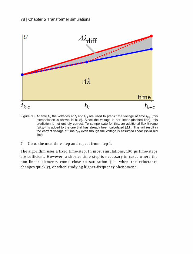
78 | Chapter 5 Transformer simulations
Figure 30: At time tk, the voltages at tk and tk-1 are used to predict the voltage at time tk+1 (this extrapolation is shown in blue). Since the voltage is not linear (dashed line), this prediction is not entirely correct. To compensate for this, an additional flux linkage (𝜟𝜟𝝀𝝀diff) is added to the one that has already been calculated (𝜟𝜟𝝀𝝀). This will result in the correct voltage at time tk+1 even though the voltage is assumed linear (solid red line)
7. Go to the next time step and repeat from step 1.
The algorithm uses a fixed time-step. In most simulations, 100 µs time-steps are sufficient. However, a shorter time-step is necessary in cases where the non-linear elements come close to saturation (i.e. when the reluctance changes quickly), or when studying higher-frequency phenomena.
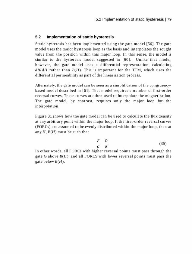
5.2 Implementation of static hysteresis | 79
5.2 Implementation of static hysteresis Static hysteresis has been implemented using the gate model [56]. The gate model uses the major hysteresis loop as the basis and interpolates the sought value from the position within this major loop. In this sense, the model is similar to the hysteresis model suggested in [60]. Unlike that model, however, the gate model uses a differential representation, calculating dB/dH rather than B(H). This is important for the TTM, which uses the differential permeability as part of the linearization process.
Alternately, the gate model can be seen as a simplification of the congruency-based model described in [61]. That model requires a number of first-order reversal curves. These curves are then used to interpolate the magnetization. The gate model, by contrast, requires only the major loop for the interpolation.
Figure 31 shows how the gate model can be used to calculate the flux density at any arbitrary point within the major loop. If the first-order reversal curves (FORCs) are assumed to be evenly distributed within the major loop, then at any H, B(H) must be such that
𝐹𝐹𝐺𝐺
=𝐷𝐷𝐸𝐸
. (35)
In other words, all FORCs with higher reversal points must pass through the gate G above B(H), and all FORCS with lower reversal points must pass the gate below B(H).

80 | Chapter 5 Transformer simulations
Figure 31: The Gate model. (a) shows the principle of the gate and how the ratios F/G and D/E must remain equal. (b) defines all the points on the major loop needed for the calculation of B(H). The values A, Arev, C, and Crev all denote the value of the flux density at the given point on the major loop. Therefore, they are all functions of H. Note that the calculated curve (blue) in (b) lies on the FORC shown in (a).
The gate model as described in [56] assumes that the hysteresis loop is a first-order reversal curve, but it can easily be adapted to apply to any reversal curve. For a first-order reversal curve, 𝐶𝐶rev = 𝐵𝐵rev, and the variables described in Figure 31 are related as
𝐷𝐷 = 𝐵𝐵rev − (−𝐵𝐵s), 𝐸𝐸 = 𝐶𝐶 − (−𝐵𝐵s), 𝐹𝐹 = 𝐵𝐵 − 𝑁𝑁, 𝐺𝐺 = 𝐶𝐶 − 𝑁𝑁.
(36)
Together with (35), this gives the flux density
𝐵𝐵 = 𝐵𝐵(𝐻𝐻) =(𝐵𝐵rev + 𝐵𝐵s)(𝐶𝐶 − 𝑁𝑁)
𝐶𝐶 + 𝐵𝐵s+ 𝑁𝑁. (37)
5.2 Implementation of static hysteresis | 81
If the curve is not a first-order reversal curve, 𝐶𝐶rev ≠ 𝐵𝐵rev, and this means that D is not given directly. It can easily be found, however, since a static curve that is not a first-order reversal curve is nevertheless part of a first-order reversal curve (see the dashed part of the calculated curve in Figure 31 (b)). D can therefore be found by extrapolating backwards to the major loop. This is done by defining a new, temporary, gate at 𝐻𝐻 = 𝐻𝐻rev. Denoting the variables of this temporary gate by primed variables,
𝐸𝐸′ = 𝐶𝐶rev − (−𝐵𝐵𝑠𝑠), 𝐹𝐹′ = 𝐵𝐵rev − 𝑁𝑁rev, 𝐺𝐺′ = 𝐶𝐶rev − 𝑁𝑁rev.
(38)
Using 𝐹𝐹′
𝐺𝐺′= 𝐷𝐷
𝐸𝐸′, this gives
𝐷𝐷 =(𝐵𝐵rev − 𝑁𝑁rev)(𝐶𝐶rev + 𝐵𝐵s)
𝐶𝐶rev − 𝑁𝑁rev. (39)
Introducing this value of D into (35) and (36) gives
𝐵𝐵(𝐻𝐻) =(𝐵𝐵rev − 𝑁𝑁rev)(𝐶𝐶rev + 𝐵𝐵s)(𝐶𝐶 − 𝑁𝑁)
(𝐶𝐶rev − 𝑁𝑁rev)(𝐶𝐶 + 𝐵𝐵s) + 𝑁𝑁 (40)
This expression can then be differentiated with regard to H, as required by the TTM. The differentiation can be simplified by considering that A and C are all points on the major loop, and that the major loop is symmetric, i.e. that the rising and falling branches are equal. Then, by using one branch 𝐵𝐵𝑆𝑆,maj(𝐻𝐻) of the major loop , the variables in Eq. (40) can be expressed as
𝑁𝑁 = 𝐵𝐵𝑆𝑆,maj(±𝐻𝐻), 𝑁𝑁rev = 𝐵𝐵𝑆𝑆,maj(±𝐻𝐻rev), 𝐶𝐶 = −𝐵𝐵𝑆𝑆,maj(∓𝐻𝐻), 𝐶𝐶rev = −𝐵𝐵𝑆𝑆,maj(∓𝐻𝐻𝑟𝑟𝑒𝑒𝑟𝑟).
(41)
The upper signs correspond to an increasing flux density and the lower signs correspond to a decreasing flux density. Introducing 𝛿𝛿𝐻𝐻 as a small change in magnetizing field, (40) can be differentiated numerically with respect to H:
𝑑𝑑𝐵𝐵𝑑𝑑𝐻𝐻
�𝐻𝐻≈𝐵𝐵(𝐻𝐻 + 𝛿𝛿𝐻𝐻) − 𝐵𝐵(𝐻𝐻 − 𝛿𝛿𝐻𝐻)
2𝛿𝛿𝐻𝐻. (42)

82 | Chapter 5 Transformer simulations
The notation can be shortened by modifying (41),
𝑁𝑁+ = 𝐵𝐵𝑆𝑆,𝑚𝑚𝑚𝑚𝑖𝑖(±𝐻𝐻 + 𝛿𝛿𝐻𝐻), 𝑁𝑁− = 𝐵𝐵𝑆𝑆,𝑚𝑚𝑚𝑚𝑖𝑖(±𝐻𝐻𝑟𝑟𝑒𝑒𝑟𝑟 − 𝛿𝛿𝐻𝐻), 𝐶𝐶+ = −𝐵𝐵𝑆𝑆,𝑚𝑚𝑚𝑚𝑖𝑖(∓𝐻𝐻 − 𝛿𝛿𝐻𝐻), 𝐶𝐶− = −𝐵𝐵𝑆𝑆,𝑚𝑚𝑚𝑚𝑖𝑖(∓𝐻𝐻𝑟𝑟𝑒𝑒𝑟𝑟 + 𝛿𝛿𝐻𝐻).
(43)
Combining (40) and (42) then gives
𝑑𝑑𝐵𝐵𝑑𝑑𝐻𝐻
�𝐻𝐻
=�(±𝐵𝐵𝑟𝑟𝑒𝑒𝑟𝑟 − 𝐶𝐶𝑟𝑟𝑒𝑒𝑟𝑟)(𝐵𝐵𝑠𝑠 + 𝐶𝐶𝑟𝑟𝑒𝑒𝑟𝑟)
𝐶𝐶𝑟𝑟𝑒𝑒𝑟𝑟 − 𝑁𝑁𝑟𝑟𝑒𝑒𝑟𝑟�𝐶𝐶
+ − 𝑁𝑁+𝐶𝐶+ + 𝐵𝐵𝑠𝑠
− 𝐶𝐶− − 𝑁𝑁−𝐶𝐶− + 𝐵𝐵𝑠𝑠
��
2𝛿𝛿𝐻𝐻
+(𝑁𝑁+ − 𝑁𝑁−)
2𝛿𝛿𝐻𝐻.
(44)
The drawback of this model is that it becomes less correct for high values of Brev, i.e. for reversal points far from the ascending branch of the major loop. This becomes an issue during startup as it leads to a significant DC offset when starting from zero flux and zero magnetizing field. For this reason, it is usually better to choose a starting H that lies on or close to the major loop in order to reduce the time required to get rid of the DC offset.
The misrepresentation of minor loops with high Brev also leads to the simulation underestimating the losses for flux with a high harmonic content. Similarly, the gate model is not suitable when simulating high-frequency transients. Neither of these shortcomings is of major concern for studying power transformers at no-load, but they are worth remembering.
The main advantage of the gate model is its simplicity. The results could undoubtedly be improved by using a more advanced model, particularly one that includes magnetization in the transverse and out-of-plane directions [62]. However, accurate models of hysteresis are complicated, often to the point of being useable only in very simple geometries. For modeling transformers at no-load, the gate model is usually sufficient.

5.3 Implementation of dynamic hysteresis | 83
5.3 Implementation of dynamic hysteresis The original TTM included only static hysteresis. As described in 5.1, dynamic hysteresis can be included, but the eddy currents must then be treated as actual currents rather than as direct contributions to the hysteresis. This is done by connecting a single-turn eddy-current winding in series with each non-linear element. Each of these eddy-current windings has an associated resistance, Reddy, in the electrical circuit. The value of Reddy is
𝑅𝑅𝑒𝑒𝑜𝑜𝑜𝑜𝑒𝑒 =
𝑈𝑈𝑒𝑒𝑜𝑜𝑜𝑜𝑒𝑒𝐼𝐼𝑒𝑒𝑜𝑜𝑜𝑜𝑒𝑒
=𝑑𝑑Φ𝑑𝑑𝜕𝜕
𝑙𝑙𝑚𝑚𝐻𝐻𝑒𝑒𝑜𝑜𝑜𝑜𝑒𝑒
. (45)
As described in chapter 2.2.2, the H-field caused by the eddy currents is a function of the flux density,
𝐻𝐻𝑒𝑒𝑜𝑜𝑜𝑜𝑒𝑒 =𝑑𝑑2
12𝜌𝜌𝑑𝑑𝐵𝐵𝑑𝑑𝜕𝜕
+𝑛𝑛0𝑉𝑉0
2��1 +
4𝐺𝐺𝐺𝐺𝑑𝑑𝜇𝜇0𝜌𝜌𝑛𝑛02𝑉𝑉0
𝑑𝑑𝑑𝑑𝑑𝑑𝜕𝜕
− 1�, (46)
The first term in (46) is the classical eddy current field, and the second term is the excess, or anomalous, eddy current field. V0 and n0 are phenomenological constants, and can be approximated through a rather complicated procedure by varying the amplitude and frequency of the magnetization. However, in this work, V0 was arbitrarily set to 3000 Am-1, and n0 was adjusted to give the correct total hysteresis losses over a period. This may seem a bit sloppy, but the result varies only very weakly with the values of V0 and n0, as long as the product V0n0 is correct. Both V0 and n0 should also depend on the magnetization [63] 19. This dependence is also weak, however, and has been ignored. It might need to be considered in simulations involving a wider range of frequencies or flux densities.
19 In the cited article, the entire excess eddy loss is lumped into a single parameter, which is then found to vary with the flux density. The principle is the same, however.

84 | Chapter 5 Transformer simulations
Assuming that the magnetization can be rewritten as 𝜇𝜇0𝑑𝑑 = 𝐵𝐵 − 𝜇𝜇0𝐻𝐻, and changing the derivatives to differences, the eddy current resistances, as they are used in the program, become:
𝑅𝑅𝑒𝑒𝑜𝑜𝑜𝑜𝑒𝑒
=
𝑁𝑁𝑒𝑒𝑠𝑠𝑙𝑙𝑚𝑚
Δ𝐵𝐵Δ𝜕𝜕
𝑑𝑑212𝜌𝜌
Δ𝐵𝐵Δ𝜕𝜕 + 𝑛𝑛0𝑉𝑉0
2 ��1 + 4𝐺𝐺𝐺𝐺𝑑𝑑𝜌𝜌𝑛𝑛02𝑉𝑉0
�(Δ𝐵𝐵 − 𝜇𝜇0Δ𝐻𝐻)Δ𝜕𝜕 � − 1� 𝑒𝑒𝑖𝑖𝑠𝑠𝑛𝑛(Δ𝐵𝐵 − 𝜇𝜇0Δ𝐻𝐻)
(47)
An advantage of treating the eddy currents as actual currents is that this, at least partially, accounts for the magnetizing effect of the eddy currents. An eddy current, just like any current around the core, causes a magnetizing field that counteracts the applied field. The magnetizing field from the eddy currents can often be larger than that from the static hysteresis, and this changes the magnetizing characteristics. However, in the method described here, this magnetizing field is treated as a leakage field, and thus included in the model.
In this way, each non-linear reluctance element is treated as a combination of three elements: a non-linear reluctance describing the static hysteresis, a single-turn winding connected to a variable resistance describing the eddy currents, and a linear air reluctance describing the leakage flux. This combined non-linear element, shown in Figure 32, is the basic building block of the TTM. The single-turn winding is treated just like the physical windings (see chapter 5.1): as a flux source in the magnetic circuit, and as a controlled current-source in the electrical circuit.

5.4 Modeling of the major loop | 85
Figure 32: Magnetic reluctance (a), represented as a flux source in series with a static hysteresis element, and in parallel with a linear leakage reluctance. In the electrical circuit (b), this corresponds to a dependent current source and a variable eddy current resistance.
The linear reluctance is also necessary in order to stabilize the simulation. If two winding elements are connected in series without a leakage path, the simulation quickly becomes unstable and crashes. In accordance with Kirchhoff’s current law, the flux in two series-connected flux sources must be exactly the same. In the simulation, this is very unlikely. Even in an ideal case, where the fluxes actually are equal, the finite numerical precision will quickly lead to small variations, which destabilize the simulation.
5.4 Modeling of the major loop Since the major loop is such an integral part of the hysteresis model, it is necessary to have a major loop that closely resembles the true major loop. This is, however, difficult to do in practice. In order to reach saturation, it is necessary to have magnetizing fields of several kA/m. At the same time, the magnetizing voltage should be kept low in order to avoid dynamic effects. This is not an insurmountable problem, but most standard single sheet testers are not built to handle these conditions. It is therefore difficult to reach much higher than 1.9 T when measuring static hysteresis. When measuring dynamic loops, however, and when magnetizing large transformers, the flux density can quite easily reach higher values. To be able to simulate these conditions, the static hysteresis loop must be extrapolated.

86 | Chapter 5 Transformer simulations
There are several methods of performing this extrapolation, with the most common being the Langevin function [64],
ℒ(𝑥𝑥) = coth(𝑥𝑥) −1𝑥𝑥
, (48)
which is used e.g. in the Jiles-Atherton model of hysteresis [65]:
𝑑𝑑 = ℒ �𝐵𝐵e𝑙𝑙� ∓ 𝑘𝑘 �
𝑑𝑑ℒ �𝐵𝐵e𝑙𝑙 �𝑑𝑑𝐵𝐵e
−𝑑𝑑ℒ �
𝐵𝐵𝑒𝑒,𝑚𝑚𝑚𝑚𝑚𝑚𝑙𝑙 �
𝑑𝑑𝐵𝐵e� + 𝑘𝑘2
𝑑𝑑2ℒ �𝐵𝐵e𝑙𝑙 �(𝑑𝑑𝐵𝐵e)2 . (49)
In this expression, 𝐵𝐵e is the effective flux density, k is a material parameter, and 𝑙𝑙 = 𝑘𝑘𝐵𝐵𝑇𝑇/𝑚𝑚, where 𝑘𝑘𝐵𝐵 is Boltzmann’s constant, T is the temperature, and m is the per-volume magnetization.
There are, however, some drawbacks to this method. Firstly, while the Langevin function is derived analytically from basic quantum mechanical theory, it is derived for paramagnetic materials. In order to describe ferromagnetic hysteresis it must be modified (as in the Jiles-Atherton model), making it an empirical approximation rather than an exact physical description. Secondly, it is expressed in terms of flux density and magnetization, rather than in terms of flux density and magnetizing field. While more correct, this is impractical from an engineering point of view, since the magnetization cannot be measured directly in a transformer. Finally, the expression is self-referring; since both 𝐵𝐵e and k depend on the magnetization, (49) gives M = M(B,M), which makes it difficult to use.
In some literature, these issues are simply ignored and the Langevin function is used to get the proper curve shape B(H), and the curve is then shifted by a constant 𝐻𝐻c in order to get a hysteretic loop. This, however, gives a rather poor agreement with measured curves.
To remedy this and get a reasonably correct static major loop to use in the simulations, a curve-fitting expression was developed [9]. The primary aims were to find an expression that accurately models measured static curves. It should also do so with a minimum of variables, and with variables that are

5.4 Modeling of the major loop | 87
fairly constant for all measurements. A model fulfilling these objectives could then be extrapolated in order to find the major loop.
For paramagnets, the shape of the magnetization curve can be determined analytically. In a paramagnet with Zeeman energy (normalized to the Boltzmann energy 𝑘𝑘B𝑇𝑇) EZ, and total magnetic moment 𝐽𝐽 (𝐽𝐽 = 1
2𝑛𝑛,𝑛𝑛 ∋ positive integers), the total magnetization is described by the
Brillouin function [66], [67]:
𝐵𝐵𝐽𝐽(𝑥𝑥) =2𝐽𝐽 + 1
2𝐽𝐽coth �
2𝐽𝐽 + 12𝐽𝐽
𝐸𝐸Z� −12𝐽𝐽
coth �12𝐽𝐽𝐸𝐸Z� (50)
As the number of possible states becomes large, i.e. for large samples, this expression becomes the Langevin function with x = EZ.
Since magnetization is a statistical process, it is reasonable to assume that some probability distribution could be used to describe it. Unfortunately, the Brillouin function does not have the correct shape for transformer steel. Another class of distributions that could be suitable are the stable distributions [68].
Three of the stable distributions, the Gaussian, Cauchy and Lévy distributions, can be expressed in closed form. Most stable distributions, however, can not, and they must therefore be defined through their characteristic functions. For a random variable X with distribution F(x), the characteristic function is
𝜙𝜙(𝑢𝑢) = � exp(j𝑢𝑢𝑥𝑥) 𝑑𝑑𝐹𝐹(𝑥𝑥)∞
−∞
. (51)

88 | Chapter 5 Transformer simulations
The characteristic function can be given in several different ways, one of which will be shown here. In the so-called “1” parametrization, the stable distribution with parameters 𝛼𝛼,𝛽𝛽, 𝛾𝛾, and 𝛿𝛿 is 𝑆𝑆(𝛼𝛼,𝛽𝛽, 𝛾𝛾, 𝛿𝛿, 1) [68]. The characteristic function that describes S is then
𝜙𝜙(𝑢𝑢)
=
⎩⎪⎨
⎪⎧exp �−𝛾𝛾𝛼𝛼|𝑢𝑢|𝛼𝛼 �1 − 𝑗𝑗𝛽𝛽 𝜕𝜕𝑙𝑙𝑛𝑛 �
𝜋𝜋𝛼𝛼2� sign(𝑢𝑢)� + 𝑗𝑗𝛿𝛿𝑢𝑢� 𝛼𝛼 ≠ 1
exp �−𝛾𝛾|𝑢𝑢| �1 −𝑗𝑗2𝛽𝛽𝜋𝜋
sign(𝑢𝑢) log(|𝑢𝑢|)� + 𝑗𝑗𝛿𝛿𝑢𝑢� 𝛼𝛼 = 1. (52)
With H as the variable, the cumulative distribution function 𝑆𝑆CDF(𝐻𝐻;𝛼𝛼,𝛽𝛽, 𝛾𝛾, 𝛿𝛿; 1) has a sigmoid shape and can therefore provide a fairly good fit for the major hysteresis loop. For the studied steels, the best fit was found by setting 𝛼𝛼 = 0.45 and 𝛽𝛽 = 1, and then varying the scale parameter γ. The location parameter δ determines the coercivity, and should be equal to the coercive field Hc.
Figure 33: Measured and fitted static hysteresis curves at 1.9 T. Unless the Brillouin function 𝐵𝐵𝐽𝐽=1(𝑥𝑥) is included, the curve is too steep.

5.4 Modeling of the major loop | 89
However, close to the zero-crossing, the fit is worse, and it becomes necessary to introduce an additional compensation term. In this case, the compensation was made by multiplying the stable distribution function by a Brillouin function 𝐵𝐵𝐽𝐽=1(𝑥𝑥) (marked in (53)). This makes the curve less steep close to 𝐻𝐻c (see Figure 33). Additionally, the shape of the curve is different for positive and negative B, and the expression must therefore have two terms: one for each half-plane. Thus, the expression for the rising branch of the major loop becomes
𝐵𝐵 − 𝜇𝜇0𝐻𝐻 = 𝑁𝑁1𝑆𝑆CDF(−𝐻𝐻;𝛼𝛼, 1, 𝛾𝛾1,−𝐻𝐻c; 1)𝐵𝐵𝐽𝐽=1�𝑞𝑞1(𝐻𝐻 − 𝐻𝐻c)��������������
compensating term
+ 𝐵𝐵𝑠𝑠𝑆𝑆CDF(𝐻𝐻;𝛼𝛼, 1, 𝛾𝛾2,𝐻𝐻c; 1)𝐵𝐵𝐽𝐽=1�𝑞𝑞2(𝐻𝐻 −𝐻𝐻c)��������������compensating term
.
(53)
The amplitude factor A1 can be deduced from the reversal point. At the reversal point, the hysteresis loop must be closed. Therefore, the first term on the right hand side of (53) must be equal to the second term, but with the opposite sign of H:
𝑁𝑁1𝑆𝑆CDF(𝐻𝐻;𝛼𝛼, 1, 𝛾𝛾1,𝐻𝐻c; 1)𝐵𝐵𝐽𝐽=1�𝑞𝑞1(𝐻𝐻 − 𝐻𝐻c)�
= 𝐵𝐵𝑠𝑠𝑆𝑆CDF(𝐻𝐻;𝛼𝛼, 1, 𝛾𝛾2,𝐻𝐻c; 1)𝐵𝐵𝐽𝐽=1�𝑞𝑞2(𝐻𝐻 − 𝐻𝐻c)� (54)
This gives A1, and the model thus has a total of six unknown fitting parameters: 𝛼𝛼, 𝛾𝛾1, 𝛾𝛾2, 𝑞𝑞1, 𝑞𝑞2, and 𝐻𝐻𝑒𝑒 .
Note that the −𝜇𝜇0𝐻𝐻 on the left hand side of (53) is the flux from the applied magnetizing field. It is very small compared to the total flux in the steel, and could therefore be neglected. An additional reason for neglecting it is that the modeling error is almost certainly larger than 𝜇𝜇0𝐻𝐻. Including it could therefore give the impression that the accuracy is higher than it really is. However, the term has been kept here for completeness.
With β = 1, the probability density function 𝑆𝑆PDF(𝐻𝐻;𝛼𝛼,𝛽𝛽, 𝛾𝛾, 𝛿𝛿; 1) is zero at 𝐻𝐻 = 𝛿𝛿. Since the cumulative distribution function 𝑆𝑆CDF(𝐻𝐻;𝛼𝛼,𝛽𝛽, 𝛾𝛾, 𝛿𝛿; 1) is the integral of the probability density function, the slope of 𝑆𝑆CDF(𝐻𝐻;𝛼𝛼,𝛽𝛽, 𝛾𝛾, 𝛿𝛿; 1), and thus of the hysteresis curve, also becomes zero at 𝐻𝐻 = 𝛿𝛿 = 𝐻𝐻c. This is undesirable, and can be avoided by shifting the two distributions in (53)

90 | Chapter 5 Transformer simulations
relative to each other. The magnitude of the shift should be such that 𝑆𝑆PDF(𝐻𝐻;𝛼𝛼,𝛽𝛽, 𝛾𝛾, 𝛿𝛿 + shift; 1) has a maximum at 𝐻𝐻c. This shift is small (less than 1 A/m), and does not affect the curve shape to any extent, but it does make the hysteresis curve much smoother (Figure 34).
Figure 34: Approximated hysteresis curves near the zero-crossing. The maxima of the two probability density functions do not quite match. This leads to the derivative of the fitted curve being zero near at the zero-crossing (red). To avoid this, the two probability functions can be offset relative to each other (blue)
5.4.1 Experimental determination of the fitting parameters The static magnetization curves were measured for three different steel grades. The steel samples were 0.23 mm and 0.27 mm domain-refined steel (23ZDKH and 27ZDKH) and a 0.3 mm non-domain-refined steel (H100-30). The measurements were performed using standard SST-MC equipment. Additionally, static hysteresis curves for the 27ZDKH steel measured using both SST-H and SST-MC were supplied by the manufacturer.
In order to minimize dynamic effects, the time derivative of the flux density dB/dt should be kept as low as possible. In these measurements, the aim was to keep dB/dt lower than 30 mT/s. However, for some of the measurements,

5.4 Modeling of the major loop | 91
the equipment was not able to maintain this value for the entire curve. This was mainly an issue close to the zero-crossing, when the flux changes very quickly even for very small changes in H. It is unclear to what extent this lead to dynamic effects. It did, however, lead to low time resolution for part of the curve (vaguely visible in Figure 35).
Additionally, the ends of the yokes of the SST are not entirely flat where they grip the sample. This leads to short air gaps in the magnetic path, and a higher reluctance. This can be in Figure 35 seen as a decreased field at the reverse knee. Sometimes it also manifests as a forward tilt of the hysteresis loop when measured using an SST-MC, compared to an SST-H.
Figure 35: Static hysteresis loops at 1.9 T, measured using SST-H and SST-MC. The difference is mainly visible in the falling branch. The lower resolution of the SST-MC measurement is also vaguely visible near the remanence point, where the curve has a slightly jagged look (arrow). In this example, the effect is rather slight, however.
For these reasons, and also owing to the inherent differences between the two measurement methods, the results are different. Where possible, the SST-H results have been used for the fitting.

92 | Chapter 5 Transformer simulations
The fitting parameters were calculated for 27ZDKH steel at 1.7 T, 1.8 T, and 1.9 T. They were then extrapolated to 2.03 T, which is the saturation flux density of the steel. As Table 6 shows, most of the fitting parameters are independent of the peak flux density or are weakly dependent. The most troubling parameter is q1, which appears to increase for higher flux density. This parameter controls the steepness of the falling branch below the reverse knee.
Table 6: Fitting parameters for 27ZDKH steel. The values up to 1.9 T are fitted to measurements, and the values for 2.03 T are an approximate extrapolation.
1.7 T 1.8 T 1.9 T 2.03 T
α 0.45 0.45 0.45 0.45
γ1 0.5 0.35 0.35 0.35
γ2 2 2 2 2
q1 0.45 0.45 0.86 0.86
q2 0.45 0.45 0.45 0.45
Hc 5.5 6.2 6.4 6.5
As can be seen in Figure 36, the fit generally agrees well with measurements. There are still some issues at the zero-crossing. Here, the flux changes quickly, and a small error in H therefore leads to a large error in B. The fit is also worse for the 1.7 T and 1.8 T curves in the region from -20 A/m to 0 A/m. Apart from this, however, the fit stays within 0.02 T of the measured values.
For comparison purposes, the figure also includes a best fit for the 1.9 T curve using the Langevin function (48). The expression for this fitting function is
𝐵𝐵 − 𝜇𝜇0𝐻𝐻 =
⎩⎨
⎧𝑙𝑙1 �coth �𝐻𝐻 − 𝐻𝐻𝑒𝑒𝑙𝑙2
� −𝑙𝑙2
𝐻𝐻 − 𝐻𝐻𝑒𝑒� ,𝐻𝐻 > 𝐻𝐻𝑒𝑒
𝑙𝑙3 �coth �𝐻𝐻 − 𝐻𝐻𝑒𝑒𝑙𝑙4
� −𝑙𝑙4
𝐻𝐻 − 𝐻𝐻𝑒𝑒� ,𝐻𝐻 < 𝐻𝐻𝑒𝑒
. (55)

5.4 Modeling of the major loop | 93
This expression has five fitting parameters20: 𝑙𝑙1, 𝑙𝑙2, 𝑙𝑙3, 𝑙𝑙4, and 𝐻𝐻𝑒𝑒. This is one parameter less than the six parameters used in the proposed fitting method. The fit is, however, significantly worse than that of the proposed method.
Figure 36: Curve fitting error compared to measured static hysteresis curves. The static curve was measured at 1.9 T, 1.8 T, and 1.7 T peak flux density. The plot also includes the error for a best fit using two Langevin functions. This is shown only for 1.9 T peak flux density. For magnetizing fields close to 𝐻𝐻c, the fit is poor for all models. However, as long as the fit is good for the rest of the curve, this is not a major limitation.
The only difference between 23ZDKH and 27ZDKH is the thickness, and this should not noticeably affect the static hysteresis. Measurements performed using an SST-MC support this.
The H100-30 steel, on the other hand, is not domain-refined, and therefore has a different magnetization behavior. However, the differences between the magnetization curves of the steel grades H100-30 and 27ZDKH are very
20 In theory, 𝑙𝑙1 should be equal to 𝐵𝐵s . This does not give the best fit, however, and 𝑙𝑙1 is therefore left as a variable.

94 | Chapter 5 Transformer simulations
similar to the differences between the magnetization curves of the measurement methods SST-H and SST-MC. The static hysteresis loop of H100-30 as measured with the SST-MC is close to that of 27ZDKH as measured with the SST-H. This makes it difficult to distinguish what part of the difference is related to the steel and what is related to the measurement device. Until further measurements can be performed, the parameters in Table 6 will be used for the non-domain-refined steels as well, even though this is not a satisfactory solution.
5.5 Modeling parallel reluctance elements The simulation can be further improved by dividing the geometry into parallel, interconnected paths. This increases the resolution of the model, and allows different flux density in different parts of the core. For example, the flux density in the inner part of the core, close to the window, is usually higher than in the outer part, on account of the magnetic path length being shorter (see Figure 37).
Figure 37: Finite element simulation of an EY core. Even though the resolution is coarse, it is clear that the flux density is higher close to the core windows.
Including additional elements in the TTM is just a matter of expanding the incidence matrix in (29), but there are some additional factors that must be considered. First of all, the physical dimensions must be correct. If the

5.6 Initial magnetization and inrush currents | 95
number of elements is so large that the model approaches a finite element model, the physical dimensions of each element are well-defined. Similarly, if only one element per limb is used, defining the dimensions is also fairly straightforward. With an intermediate number of elements, it is not always clear what size each element should be or, conversely, which part of the core should be included in each element.
In most cores, the limbs are approximately cylindrical, and the yokes are semi-cylinders. Since the TTM, as implemented here, does not consider out-of-plane flux, the connections between the limbs and yokes can not be entirely correct. In the simulations shown in this thesis, the cross-section has been approximated as square for the purpose of determining their sizes. All magnetic lengths have then been scaled down in order to give the correct total core volume.
The second factor to be considered is that if a winding is split into several parallel elements, the mmfs in all the winding elements must be the same. This is handled easiest by drawing out all parallel winding elements to the electrical circuit and connecting them there.
5.6 Initial magnetization and inrush currents In order to get the correct behavior for the magnetization current, the initial magnetization state of the core must be correct. Otherwise, the magnetizing field will not match the flux density. This kind of mismatch leads to a DC component in the current. The DC component decays over time, but this drastically increases the required calculation time. To avoid this, a constant voltage is applied at the beginning of the simulation in order to bring the magnetization to a correct value.
This voltage is applied for a short time, corresponding to an electrical angle of 1 radian. The magnitude is chosen such that at the end of this time, the flux in the winding is at its rated value. This method ensures that the flux and static hysteresis field will be correct. The choice of time period also gives a rate of change of the flux that is close to what the core would experience during normal operation at sinusoidal voltage. This ensures that the dynamic

96 | Chapter 5 Transformer simulations
hysteresis is also approximately correct. An example of this start-up method can be seen in Figure 38.
Figure 38: Currents (solid) and flux densities (dashed) during the first period after the start-up. The flux ramp continues until approximately 0.0032 s, after which point the normal, sinusoidal magnetization starts. Even with this start-up method, there is a small DC component. This is particularly visible in the blue phase, which is not symmetric in the positive and negative half-periods.
In addition to this start-up method, there are two other methods that are relevant to this work. The first is to run a simulation for a long time to let the DC decay, and then use the final values of that simulation as starting values for further simulations. This is only useful in cases where several simulations are run with the exact same starting state, e.g. for transient simulations. This thesis is only concerned with steady-state operation, however, and this start-up method has therefore not been pursued further.
A second alternative is to apply a sinusoidal voltage and slowly increase the voltage from zero to the rated voltage. This is the method used during testing of real transformers. It is time-consuming, however; during a transformer test, it can take several minutes to ramp up to rated voltage. Additionally, it

5.7 Simulation results, single phase | 97
is mathematically difficult to find a ramp shape that does not, by itself, give a DC contribution.
With voltage 𝑈𝑈(𝜕𝜕) ~ cos (𝜔𝜔𝜕𝜕), the ramp can be written as 𝑈𝑈ramp(𝜕𝜕) =𝑓𝑓(𝜕𝜕)cos (𝜔𝜔𝜕𝜕) for some function 𝑓𝑓(𝜕𝜕). At the end of the ramp, 𝜕𝜕 = 𝜕𝜕end, the integral of 𝑈𝑈ramp(𝜕𝜕) must be exactly equal to the flux density,
𝐵𝐵(𝜕𝜕end) = � 𝑓𝑓(𝜕𝜕) cos(𝜔𝜔𝜕𝜕) 𝑑𝑑𝜕𝜕.
𝑡𝑡end
0
(56)
Additionally, in order to avoid a discontinuity in the voltage, 𝑈𝑈ramp(𝜕𝜕end) must be proportional to 𝑈𝑈(𝜕𝜕end). With an appropriate choice of 𝜕𝜕end, it is possible to find an 𝑓𝑓(𝜕𝜕) that fulfills these criteria. However, for a three-phase transformer, the criteria must be simultaneously fulfilled in all three phases. No such function has been found, and this start-up method has therefore not been used in the simulations.
Regardless of which start-up method is used, a small DC component is unavoidable. This is because of the non-linear relationship between voltage and current in the transformer. In order to predict the magnetization current with perfect accuracy, it would be necessary to predict the relationship between voltage and current at every point during the start-up process. Any start-up method capable of this would be superior to the simulation method itself. It would therefore be unnecessary to develop the simulation in the first place.
5.7 Simulation results, single phase When it comes to accuracy, the type of transformer model is generally less important than how the core is modeled and which magnetization phenomena are included. In many cases, it is possible to determine, just by looking at the no-load currents from a transformer model, how the magnetization was modeled and which simplifications were made. For this reason, a few pages will be dedicated to illustrating how different assumptions affect the results. This will be done using the TTM, but with different simplifications and assumptions. The benchmark for these

98 | Chapter 5 Transformer simulations
examples will be a measurement on unit 2. The full model used in this thesis will then be further elaborated with additional examples.
Visual inspection of hysteresis curves is often the best way of assessing any deviations from the expected in a quick and qualitative manner. On the other hand, for more exact, quantitative evaluation, a mathematical expression must be used. Here, the root-mean-square difference between the simulated and measured currents,
Δ𝐼𝐼rms = �1𝑇𝑇� (𝐼𝐼meas − 𝐼𝐼sim)2𝑑𝑑𝜕𝜕 𝑇𝑇
0�
12
, (57)
is used. Expressed as a percentage of the measured rms current, this gives an estimate of the simulation error. Another alternative is to use the maximum difference between measurement and simulation. This alternative is, however, more sensitive to variations in peak flux density. Small variations in Bpeak lead to very large differences in Hpeak, but do not affect the rest of the curve to the same extent. Using the maximum difference therefore tends to overestimate the simulation error.
5.7.1 Anhysteretic magnetization The simplest way to model non-linear magnetization is to ignore hysteresis. Actually constructing an anhysteretic curve is not as trivial as it may seem. Anhysteretic curves have been the subject of several studies, and several ways of constructing them have been suggested [69].
One way is to use the virgin curve, where the steel is magnetized from a completely demagnetized state. This procedure is fairly simple, and gives a curve that is anhysteretic. However, the virgin curve quickly approaches the hysteretic curve. This gives a very low differential permeability at low flux densities. This is usually not desirable. Other ways are tracing a line through the middle of a hysteretic curve (e.g. the major loop), or measuring several hysteretic curves at different peak flux densities and taking the reversal points as the anhysteretic curve. These methods all give anhysteretic curves that have some relation to the hysteretic curve.

5.7 Simulation results, single phase | 99
To avoid the influence of hysteresis, a more rigorous method is to use a constant magnetizing field HDC with a superimposed varying field HAC [70]. The varying field is then slowly decreased to zero. This leaves only the flux density corresponding to the constant magnetizing field. The procedure is repeated for a large number of constant fields, and the anhysteretic curve is taken as the interpolation between these points.
This method is time-consuming, however. Additionally, transformer cores are hysteretic, and an anhysteretic curve is not expected to be able to model them correctly. In this thesis, the anhysteretic curve is not used except in this example. It is therefore desirable to have a method that is as simple as possible. The simplest method is to use the virgin curve. Here, the virgin curve has been derived from the DC permeability of the steel. The DC permeability curves of common transformer steels can be found in the catalogues of steel manufacturers, and the anhysteretic curve can then be calculated as B = µH.
Figure 39 shows a comparison between a simulation using this type of anhysteretic curve, and the actual transformer. As can be seen in the figure, the lack of hysteresis makes the simulation error quite large. In this case, Δ𝐼𝐼rms = 87 %. As a fast approximation, or in cases when the hysteresis is not interesting (such as at high saturation), however, it can give the basic wave-shape.
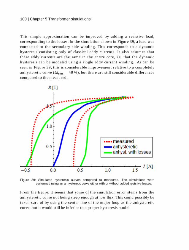
100 | Chapter 5 Transformer simulations
This simple approximation can be improved by adding a resistive load, corresponding to the losses. In the simulation shown in Figure 39, a load was connected to the secondary side winding. This corresponds to a dynamic hysteresis consisting only of classical eddy currents. It also assumes that these eddy currents are the same in the entire core, i.e. that the dynamic hysteresis can be modeled using a single eddy current winding. As can be seen in Figure 39, this is considerable improvement relative to a completely anhysteretic curve (Δ𝐼𝐼rms = 40 %), but there are still considerable differences compared to the measured.
Figure 39: Simulated hysteresis curves compared to measured. The simulations were performed using an anhysteretic curve either with or without added resistive losses.
From the figure, it seems that some of the simulation error stems from the anhysteretic curve not being steep enough at low flux. This could possibly be taken care of by using the center line of the major loop as the anhysteretic curve, but it would still be inferior to a proper hysteresis model.

5.7 Simulation results, single phase | 101
5.7.2 Hysteresis based on SST measurement Before implementing the hysteresis model, it is worthwhile to study what would happen if the dynamic hysteresis curve, as measured using an SST, were used directly. This type of comparison is only possible in simple cases, where the flux is homogenous and sinusoidal throughout the entire core. This might seem like a strict requirement, but it is fulfilled in many single-phase transformers, at least to a first approximation. It is therefore reasonable to assume that hysteresis curves from SST measurements should be close to those measured on such transformers. Figure 40 shows such a comparison. Since this is not really a simulation of the transformer, the B-H curve has been plotted, rather than the B-I curve as in the other figures. The magnetizing field is calculated using the path length approximation described in chapter 4.1. Accordingly, the difference between the two measurements is expressed as Δ𝐻𝐻rms = 27 %.
Figure 40: Hysteresis curve of a large power transformer compared the hysteresis curve measured using an SST-MC. Note that, unlike the other plots, the x-axis here shows H.

102 | Chapter 5 Transformer simulations
From the figure, it can be seen that the SST requires a higher magnetizing field to reach the same flux density. This is likely linked to the magnetization of the yoke of the SST. Even though the core is much thicker than the sample, and therefore magnetized to a much lower extent, it still requires a certain magnetizing current. Additionally, small air gaps between the sample and the yoke are unavoidable, and will also contribute to the SST itself drawing a magnetizing current in addition to that required by the sample.
In any case, the hysteresis curve of the material itself is of limited use. Even if it were absolutely identical to the transformer curve, it could still not be used to model transformers with more complex core geometries or for three-phase transformers.
Similarly, an actual measurement of the no-load behavior of a transformer could be used as the basis for a simulation of that transformer. This can give very accurate results [71], [72], but it requires a measurement of the transformer. Thus, the technique is mainly useful for modelling healthy transformers under abnormal conditions. Since this thesis focuses on determining the health of transformers under normal conditions, this technique can not be used here.
5.7.3 Hysteresis based on approximated major loop By implementing the hysteresis model described in chapters 0-5.4, the simulation can be used for more complicated transformer geometries, and the results become slightly more accurate. As shown in Figure 41, the agreement is now better (Δ𝐼𝐼rms = 40 %), but the simulation saturates too late (the knee occurs at a too high flux density), and too heavily (the peak field is too high).

5.7 Simulation results, single phase | 103
Figure 41: Measured and simulated hysteresis curves of Unit 1. The simulation is performed using the gate model.
5.7.4 Parallel reluctance elements As described in chapter 5.5, the flux does not distribute evenly in the core. By taking this into account, the simulation can be further improved. Figure 42 shows an example of a reluctance network for a single-phase transformer with an SR core. Since the core is symmetric, only one quarter of it has been included in the reluctance network (Figure 43).

104 | Chapter 5 Transformer simulations
Figure 42: A reluctance network with three parallel circuits. The non-linear reluctances (black) simulate the wound limb, one return limb, and two corner joints. The simulated part of the core corresponds to the blue quarter in Figure 42.
Figure 43: An SR core is symmetric both in the up-down and left-right direction. Therefore, only one quarter (blue) of the core has been simulated. The other three quarters behave identically.

5.7 Simulation results, single phase | 105
The additional corner elements make the paths longer the further out they are in the core. The paths are connected by transverse flux elements. The magnetic properties of the steel in the transverse direction are very different from those in the rolling direction, and should be modelled differently. However, in order to keep the model simple, they are modeled here as linear (air) reluctances. The dimensions of these elements turn out to not be very important. They are mainly included to make sure that the flux distributes unevenly between the non-linear elements. This happens even if the dimensions are only approximate.
As seen in Figure 44, this has the effect of making the core start to saturate at a lower flux density (I = 0.6 A at 1.3 T, compared to 0.5 A at 1.3 T in Figure 41). Additionally, the peak H-field is significantly lower. Δ𝐼𝐼rms now decreases to 14 %
Figure 44: Measured and simulated hysteresis curves of Unit 1. The simulation has been carried out using three parallel flux paths of different lengths.

106 | Chapter 5 Transformer simulations
5.7.5 Air gaps in corner joints Figure 42 shows six air gap reluctances. These are included to simulate the air gaps in the corner joints. However, it appears best to keep these elements small. Increasing the air gaps leads to a higher total reluctance, and a higher peak current in the simulation. Since the simulations already consistently give higher currents (see Figure 41 and Figure 44), this in not desired. The air gap lengths have therefore been set to 1 µm in all the single-phase simulations.
5.7.6 The electrical circuit The electrical circuit has an impact on the simulation results, and must be modeled correctly. Unfortunately, this requires all the circuit impedances to be well known. The inductances of the generator and the step-up transformer are known, and including them further improves the simulation. In this example, Δ𝐼𝐼rms = 9 %.
However, there are additional impedances that have been neglected. For example, the capacitances of the step-up transformer have been neglected. Similarly, the impedances of the connection cables have also been neglected. To further improve the modeling of the electrical circuit, these impedances should be measured. It should also be noted that both the generator and the step-up transformer have been modeled as linear inductances. Modeling them fully, as non-linear objects, could improve the simulations further.
The additional impedances could also be approximated by setting them to values that minimize the error between simulations and measurements. In the interest of scientific rigor, however, this should be avoided. It is always possible to improve the results of a specific simulation by adapting the input parameters. However, unless those adaptations are based on actual measurements, there is no way to be certain that they are correct. They could just improve the results of the specific simulation, while making other simulations worse. For this reason, it is important to perform further studies of the measurement circuit in order to improve the simulations.

5.7 Simulation results, single phase | 107
5.7.7 Discussion With the implementation described here, the simulations do not quite reach the target accuracy, as seen in Figure 45. This is likely associated with the simplified core geometry used in the simulations. Using a larger number of reluctance elements should improve the results. Improving the hysteresis model and including all electrical impedances would also be expected to yield a slight improvement.
Figure 45: Average deviation between simulated and measured no-load currents for four single-phase power transformers. The error tends to become larger for increasing flux density due to the increasing saturation.
It should be pointed out, however, that the majority of the error is in the saturation peak. The simulation consistently gives a higher peak current than the measurement, and this has a large impact on Δ𝐼𝐼rms. Excluding the peaks, Δ𝐼𝐼rms is below 10 % for 70 % - 90 % of the period for most of the simulations, as can be seen in Figure 46.

108 | Chapter 5 Transformer simulations
Figure 46: Simulation error for Unit 2 over the course of one half-period in percent of the rms current. The error is less than 10 % for most of the half-period.
It might also be that the 10 % accuracy requirement is too strict. There is a difference even between measurements on real transformers. This can be seen, for instance, by calculating the difference between Unit 1 and Unit 2. With both units magnetized to the same flux density, Δ𝐻𝐻meas,rms is
Δ𝐻𝐻meas,rms = �1𝑇𝑇� (𝐻𝐻Unit 1 − 𝐻𝐻Unit 2)2𝑑𝑑𝜕𝜕 𝑇𝑇
0�
12
, (58)
At the rated flux density of Unit 1, Δ𝐻𝐻meas,rms = 12 %. While it is hoped that part of this difference is significant and actually due to differences between the units, the truth is that some of it is likely just due to statistical deviations.

5.7 Simulation results, single phase | 109
The simulations also neglect variations due to temperature. Both the losses and the magnetizing field vary with temperature21. For example, the studies performed in [73] suggest that the coercivity and remanence of CGO steel might decrease by ten percent or more over the temperature range found in a transformer. Though no-load testing is usually performed at room temperature, the internal temperature of the transformer can vary depending on previous tests. For example, at full load current, the hot spots in a transformer may reach almost eighty degrees above the ambient temperature. For the same reason, if measurements are performed on a unit in operation, the core temperature could be higher. The effect of temperature should therefore be included in future versions of the TTM.
The simulations consistently overestimate the losses (Figure 47). This is probably also related to the simplified geometry. However, it could also be partially due to the hysteresis curve itself. As seen in Figure 44, the simulation underestimates the magnetizing field at the reverse knee22. This behavior is intrinsic to all simulations and is due to the gate model. Measured static loops tend to follow the major loop more closely than the gate model does. This problem could potentially be solved by introducing some weighting factor into the gate model. This would, however, deprive the model of one of its strengths: its simplicity. It is also difficult to measure the major loop accurately enough to derive those weighting factors.
21 The increased resistance at higher temperature decreases eddy current losses. Higher temperature increases the permeability at low flux density, but decreases the permeability at high flux density [73]. 22 Since the simulation overestimates the losses, this does not seem to have a major impact in itself. It does, however, illustrate that the gate model has some intrinsic issues.

110 | Chapter 5 Transformer simulations
Figure 47: Simulated no-load losses in percent of the measured. The simulations consistently overestimate the losses.
Finally, the error in the simulated losses is also partially due to the fact that the excess eddy current fields have been chosen to give the correct coercivity, not the correct losses. This improves the simulations when it comes to the currents, but at the expense of the losses.
In summary, the simulations do require further improvement. Nevertheless, under certain conditions, and by compensating for the known shortcomings, they meet even relatively strict accuracy requirements.
5.8 Simulation results, three phase As with single-phase simulations, the results vary depending on the assumptions. In most cases, these variations are the same as for single-phase transformers, but there are some additional intricacies with three-phase units. Two cases in particular will be mentioned here. The first has to do with simulations using anhysteretic curves, and the second has to do with rotational magnetization in the joints.

5.8 Simulation results, three phase | 111
5.8.1 Anhysteretic magnetization in three-phase transformers When a three-phase transformer is simulated using an anhysteretic magnetization curve, the interaction between the phases tends to give the appearance of hysteresis. There may even be some simulated losses, though the phases tend to cancel out. In the simulation shown in Figure 48, there appear to be losses in phases 2 and 3 (green and blue) that are approximately 20 % of what they would be with true hysteresis. They have opposite signs23, however, and therefore cancel out. The total losses in the simulation are just a few percent of the true losses.
This is entirely an artifact of the electrical interaction between the phases, however. This interaction also makes the two outer phases mirror images of each other. This can be seen in Figure 48. In this case, the transformer is delta-connected, and the “mirrored” phases are the phases that involve the middle limb (green and blue in the figure). Phase a (red in the figure) involves only the two outer limbs, and is therefore approximately symmetric.
23 It is not uncommon to have different losses in the phases, even in measurements. In extreme cases, it is even possible to measure negative losses in one of the phases. The total losses are always correct, however.

112 | Chapter 5 Transformer simulations
Figure 48: Measured no-load currents of Unit 11 (dashed), and simulated (solid) no-load currents using an anhysteretic magnetization curve. Note that the currents shown here in green and blue are mirror images of each other (see arrows).
This behavior is characteristic of three-phase simulations with an anhysteretic magnetization curve. As with single-phase units, the simulation error becomes rather large, Δ𝐼𝐼rms ≈ 60 % in all three phases.
5.8.2 Rotational magnetization in corner joints In the joint regions of the core, and particularly in the T-joints, the flux behavior can become quite complex. Unlike most of the core, where the change of magnetization occurs mainly through domain wall movement, in the corner joints the flux must at some point change direction. This change can take place through rotation of the magnetic moments. The magnetization behavior is then different [74], [75].
The simulation model used here does not consider rotational magnetization. On a macroscopic level, it can be indirectly modeled by using additional elements for the transverse and out-of-plane flux. This can simulate the flux

5.8 Simulation results, three phase | 113
choosing different paths and rotating within the core. However, this does not account for the microscopic differences in the magnetization. Rotation of magnetic moments carries a higher energy cost and leads to higher fields. This is not considered in the model, and thus the simulation will underestimate this contribution.
5.8.3 Discussion As with the single-phase units, the simulation results differ from the measurement results by 10 % - 30 % of the rms current. Unlike the single-phase results, however, the three-phase simulations underestimate the peak currents. This can be seen in Figure 49, and becomes even more pronounced at higher flux density. The problem can be partially mitigated by decreasing the limb cross-sections in the simulation, but there is no physical reason to do so.
Figure 49: Simulated and measured no-load currents in Unit 11. The simulation underestimates the peak currents and how they interact with the other phases. This is particularly visible around 0.013 s. The average Δ𝐼𝐼𝑟𝑟𝑚𝑚𝑠𝑠 in the three phases is 12.5 %.
114 | Chapter 5 Transformer simulations
Additionally, the three-phase simulations do not overestimate the losses the way that the single-phase simulations do. This is likely connected to the simplified treatment of the joints. The specific iron losses in a three-phase transformer are usually 10 % - 20 % higher than the losses of the electrical steel. This difference, known as the building factor, is usually attributed to the rotating magnetization in the joints.
The three-phase simulations suffer from DC bias to a greater extent than the single-phase simulations do. This makes the half-periods asymmetric and increases the simulation error. As described in chapter 5.6, the bias can be minimized by using an appropriate start-up method for the simulation, but not completely avoided. The bias also decays over time. However, the time required for it to fully decay is long. A certain DC bias must therefore be expected in the simulations.
However, because the TTM uses the differential dB/dH, the offset is mainly in the current, and not in the flux. A flux offset would lead to very different peak currents in the positive and negative half-periods. A current offset, on the other hand, has only a small impact on the flux. Therefore, the DC current, calculated as the average over a period, has simply been removed during post-processing. The magnitude of the DC current varies between simulations, and between the three phases. In most cases, however, it is only a few percent of the no-load current.
It is also worth pointing out that in some cases, the measurement may have a DC bias as well. Though not directly related to the simulation, this also contributes to making the simulation error seem larger.

6 Magnetizing phenomena in real power transformers
Real power transformers differ from the usual textbook examples in some aspects. In some cases, this is because the large size of a large power transformer makes phenomena prominent that are not noticeable in smaller equipment. In other cases, the no-load currents are so low as to not warrant closer scrutiny. Unless, that is, one is specifically studying the no-load properties.
This chapter describes some of these phenomena. The chapter has been compiled from questions that have arisen during the course of the project. Some of the phenomena are directly relevant to the diagnostic method, while others are just common sources of confusion that deserve clarification.
6.1 Phase imbalance When a three-phase transformer is magnetized, there is always an imbalance between the phases. Either the sum of the phase currents is non-zero, or the sum of the phase voltages is non-zero. Of these, the case with non-zero total phase current is simpler and will be described first. The imbalance is caused by the interaction of electrical and magnetic effects in the transformer. The magnetization behavior of a core is governed by the magnetization curve of the steel in such a way that the magnetizing field is always given by the flux density. The function H(B) is history-dependent and can be quite complex, but for a given starting point and a given behavior of B, there is only one possible value of B. On the other hand, the current 𝐼𝐼 = 𝑁𝑁−1 ∮𝐻𝐻 𝑑𝑑𝑙𝑙 is defined by Kirchhoff’s law and the total current into the transformer must be zero. To fulfill both these requirements, the transformer must draw a compensating current through the neutral.

116 | Chapter 6 Magnetizing phenomena in real power transformers
Figure 50: Three identical magnetization currents with 120˚ phase shift, and the sum of currents.
Figure 50 demonstrates this effect in an ideal three-phase core where the phases are identical and do not interact. The figure has been created by taking the magnetization curve of a single-phase unit and shifting it ±120˚ to get three identical phases. In the figure, it is clear that the sum of these three currents is not zero. Indeed, the sum current has almost the same amplitude as the magnetizing current in each phase. This phenomenon is partly caused by saturation, but as Figure 51 shows, it occurs even below saturation as a consequence of hysteresis.

6.1 Phase imbalance | 117
Figure 51: Three identical magnetization currents with 120˚ phase shift, and the sum of
currents. At lower flux density
However, these figures only show what would happen if there were no other constraints on the currents. In reality, the outside impedances, and more importantly, the vector group of the transformer will also influence the currents. For example, in a three-phase transformer connected in delta or ungrounded wye, the sum current must be zero. This leads to two counteracting effects: On the one hand, the H-field is given by the core steel, depending on the flux density. On the other hand, the H-field is given by the current through Ampère’s law.
There are three possible ways of solving these, seemingly contradicting, demands. The first is to allow the flux path to change so that Ampère’s law can be fulfilled even with varying current. The second option is to allow the magnetizing voltage to vary. In this case, the flux density can vary in such a way as to eliminate the non-zero sum current. The third, and dominant, option is to allow a leakage flux in the air inside the winding. The total H-field, including the leakage fields, can then be zero while the core H-fields still adhere to the magnetization curve.

118 | Chapter 6 Magnetizing phenomena in real power transformers
In reality, all of these three effects occur to some extent. The change of magnetic path length is usually rather small, since it is constrained by the physical dimensions of the core. Due to the flux following the path of least reluctance, the shorter paths are usually more saturated and therefore more unbalanced.
Voltage variations are usually not very pronounced since the source impedance of the feeding grid is very low, and the voltage is therefore very close to sinusoidal. However, in a transformer with an ungrounded wye connection, the floating neutral allows the winding voltages to vary even though the terminal voltages are fixed. Under such conditions, the neutral point voltage can vary by up to almost one percent of the rated voltage. Nevertheless, this corresponds to only a minor change of the flux, and the main mode of regulating the sum current is still through leakage flux.
Figure 52: The flux path from one outer limb to the other is longer than the flux path from the middle limb to either of the outer limbs by an amount equal to twice the limb pitch (LP), even though the limb height (LH) is the same. Thus, the flux path of the flux from one of the outer limbs (the left limb, in this case; shown in green) is longer than that of the middle limb (red).
In addition to this imbalance caused by the hysteresis, a three-phase transformer is also imbalanced by the fact that the middle limb is magnetically shorter than the outer limbs. This is so because the return path of the middle limb flux is split between the two outer limbs while the return path of an outer limb is split between the middle limb and the other outer

6.1 Phase imbalance | 119
limb, which is substantially farther away as demonstrated in Figure 52. This can be seen in Figure 53, which is identical to Figure 51, except that the middle limb has been made 30 % shorter than the outer limbs. Consequently, the sum current is no longer just a 150 Hz sine wave.
Figure 53: Three magnetization currents with 120˚ phase shift, and the sum of currents. The middle limb (P2) has been made 30 % shorter than the outer limbs, and the magnetization current is therefore lower.
It is not just the no-load current of the middle limb that is different, however. Measurements show that all three no-load currents are different. This is because, as already described, the no-load current in a certain phase is a combination of the magnetization current in that phase, and leakage current (i.e. current caused by the leakage flux) from the other phases. Exactly how the phases interact depends on the relative reluctances and impedances in all three phases. This means that there is a preference for one phase to interact with a certain one of the other two phases during part of the period, and with the other of the two during the other part of the period. Thus, the two outer phases, even though they are magnetically identical,

120 | Chapter 6 Magnetizing phenomena in real power transformers
interact differently with the middle limb, and the no-load currents are therefore different (Figure 54).
Figure 54: Measured hysteresis curves in Unit 14. Note that all three phases are different, and that the largest difference is between the two outer phases (red and blue). The ripple in phase C (blue) is due to capacitive current, and is not relevant here.
This shows clearly why it is important to make the distinction between no-load currents (i.e. the actual measured currents) and magnetizing currents (i.e. the component of the currents that magnetize the core). It also illustrates why the no-load loss measurement generally measures different losses in all three phases. The losses are calculated by the wattmeter by multiplying the voltage and current in each phase. As discussed here, however, the no-load currents are generally not representative of the magnetization of the limbs. Thus, the no-load losses in a phase are not the same as the magnetization losses in the corresponding limb. Visual inspection of Figure 54 shows that the losses (i.e. the area of the hysteresis curve) are significantly higher in phase C than in the other phases, but also that the losses in phase B (green) are slightly higher than in phase A (red),
6.2 The impact of delta windings on the no-load current | 121
even though phase B is the middle phase and thus should have the lowest losses.
6.2 The impact of delta windings on the no-load current When a transformer is magnetized from a YN-connected winding, and one of the other windings is a delta winding, the imbalance described in the previous chapter is enhanced. This is because of the induced current in the delta.
A delta winding represents a low-impedance path for triplen harmonics (i.e. the third, ninth, fifteenth, etc.). If the neutral point on the primary side is grounded, the triplen current can become quite large. This current circulates in the delta-connected winding, and thus depends on the impedance of the delta
This is demonstrated in measurements on the distribution transformer described on page 53. The transformer was energized from the low-voltage grounded wye. The measurement was then repeated with the high-voltage delta winding open. As seen in Figure 55, the neutral current almost doubles when the delta is present. The additional current due to the delta is also shifted by 90°. This is because it is mainly resistive and limited by the delta winding resistance.

122 | Chapter 6 Magnetizing phenomena in real power transformers
Figure 55: Primary side neutral current in the distribution transformer with and without the secondary side delta.
If the neutral current can be measured without the delta winding, the neutral current with the delta present can be calculated, at least approximately [6]. From a practical viewpoint, this is not very useful, however. If it is possible to connect and disconnect the delta winding, it is probably possible to measure the current in it directly.
The distribution transformer must also be considered an extreme case since it has the delta winding on a high voltage winding with a large number of turns. The voltage driving the circulating current is therefore high, giving a high circulating current. Additionally, the high conversion ratio means that this current will be high when transferred to the low-voltage primary winding. In large power transformers, on the other hand, the delta winding is usually a low-voltage winding. The circulating current in the delta, in per-unit, is therefore much lower.

6.3 Remanence in large power transformers | 123
6.3 Remanence in large power transformers Transformers often acquire a certain remanent magnetization, either from the disconnection process, or from an earlier test involving direct current (e.g. a winding resistance measurement). When the transformer is then connected to a sinusoidal voltage, the working point will be slightly offset, resulting in an asymmetric magnetization and generation of even harmonics. There are two methods of reducing this DC bias24.
The first is through forcing the magnetization to follow the major loop. The flux density can never exceed the major loop, and therefore any DC bias that would bring it over the limit is removed. This mechanism is more useful in smaller equipment that can be fed from a controlled current source, since then the flux density can be forced to known points on both ends of the hysteresis loop, without needing to go to full saturation. By controlling the maximum magnetizing field to be the same in both the positive and negative half-period, and by choosing this value reasonably close to the major loop, the peak flux density can also be determined exactly at both ends of the hysteresis loop, thus eliminating the DC bias.
In transformers, where the voltage is the controlled quantity, this is not possible, and the reduction of the DC bias occurs instead through voltage wave-shape distortion. When the no-load current is high, the magnetizing voltage will decrease due to the voltage drop over the source impedance. This will in turn decrease the flux density, and since a DC bias leads to a higher current in one half-period, this effect will be stronger in that half-period, and thus counteract the DC bias. Since the effect is stronger the higher the voltage drop, the DC bias reduction is faster the larger the source impedance and the higher the flux density is.
One consequence of this is that transformers designed to run at lower flux densities will take longer to get rid of the DC bias, unless they are
24 Remanence also decays naturally over time. The time-scale for this mechanism is fairly long, though, and it is not relevant during testing of large power transformers.

124 | Chapter 6 Magnetizing phenomena in real power transformers
magnetized at high overvoltages, which is potentially harmful to the insulation. It also means that a testing facility with a strong voltage source and low source impedance will need more time for the remanence to decay.
Figure 56: Total amplitude of the first fifteen odd and even current harmonics. This figure shows the harmonics of phase a.
Reducing the remanence can take a long time, as shown in Figure 56. Unit 16 was magnetized to 110 % of the rated voltage and allowed to run for 30 minutes. The first 30 harmonics were divided into odd and even and summed up to give an estimate of the harmonic content. The odd harmonics decrease by approximately 25 % over the duration of the test, and approach a steady-state value25. The even harmonics, however, decrease by almost 70 % during the same time, and do not appear to reach a steady-state. Indeed, at steady-state, the even harmonics should be zero, ignoring the possibility of even harmonics actually supplied from the generator. Even after 30 minutes,
25 This is expected, since the magnetization current has a high odd-harmonic content.

6.3 Remanence in large power transformers | 125
there are more than 3 amperes of even harmonics left in the no-load current. The step seen at 585 s in the figure is caused by the voltage being changed at that point to bring it closer to the prescribed voltage for the test. The voltage was changed by less than half a percent.
Remanence is a major complication for the no-load current measurements described in this thesis. In chapter 5, the aim for the simulation method was to come within 10 % of the measured results. If remanence can make the measured result vary by significantly more than 10 %, this makes that aim difficult to fulfill. It is therefore crucial to allow the remanence to decay before performing the measurements.
Figure 57: As the remanence is worked out of the transformer, the no-load losses quickly approach their steady-state values.
At the same time, it must be pointed out that the remanence is no major issue when measuring the no-load losses. As can be seen in Figure 57, the losses vary by only a few percent, and quickly reach their steady-state value,

126 | Chapter 6 Magnetizing phenomena in real power transformers
even though there is still a high harmonic content. For this reason, it was not immediately realized how slowly the remanence can decay, and some of the measurements in this project were made with the transformer still in a remanent state.
6.4 Harmonics The current-harmonic amplitudes are sometimes measured during no-load testing of new transformers. There are two common reasons for this. The first is for setting protective relays that are sensitive to harmonic content. The other reason is power quality demands: in some instances there are limits on current harmonics as well as voltage harmonics. With the transformer operating at low load, the no-load current harmonics could cause these limits to be exceeded.
Due to the non-linear nature of the core, the behavior of the harmonics is not always easy to predict or explain. This can lead to confusion and disagreement as to whether the measured harmonic content is normal or indicative of a problem. This chapter attempts to demonstrate the most common pitfalls.
It is often assumed that having an infinite zero-sequence impedance (e.g. by having a delta or ungrounded wye connection) in a transformer will completely quench the triplen harmonics. This is, however, only an approximation. The delta winding only suppresses balanced triplen harmonics, i.e. harmonics that have the same amplitude and the same phase angle in all three phases. Transformer no-load currents are generally not balanced. If there is a non-zero total third harmonic, it cannot be completely suppressed.
Additionally, the delta winding only suppresses triplen harmonics in cases where the transformer is magnetized from the delta. If the transformer is magnetized from a YN-connected winding and the delta is the secondary (or tertiary) winding, the triplen harmonics will instead increase. In this case, delta winding provides a short-circuited path for the triplen harmonics (see chapter 6.2).

6.4 Harmonics | 127
Triplen harmonics and their impact on symmetric components are treated analytically in [76]. Building on that paper and the principles described in chapter 6.1 of this thesis, it can be found that the harmonics affect not only the currents, but also the voltages. This is because the B-H relationship in the core must always be maintained. Any decrease of the current harmonics (e.g. because of the presence of a delta winding) must come at the expense of increased flux harmonics to compensate. This in turn leads to increased voltage harmonics on the secondary side of the transformer.
The phenomena described above depend on how the transformer is connected. However, during no-load testing, the transformer is not necessarily connected the way it would be in operation, and in that case, the measured no-load currents and voltages will not be representative of what can be expected during operation.
This difference is most visible in YN/d-connected transformers, since magnetizing from the wye-connected winding causes increased triplen harmonics in the current (see section 6.2), while magnetizing from the delta suppresses the balanced triplen harmonics in the current. However, there are differences even between other vector groups.
This is demonstrated in Figure 58. The 1 MVA transformer described in section 3.4 was first magnetized with the primary connected in an ungrounded wye connection, and then later in a delta connection. With a wye-connected primary, the third current harmonic increases, while the fifth and seventh voltage harmonics decrease. Note also that, as described earlier, the third harmonic is never zero, except in one phase in the delta-connected transformer.

128 | Chapter 6 Magnetizing phenomena in real power transformers
Figure 58: Current and voltage harmonic content, in percent of the fundamental, with the primary side either delta-connected (□), or wye-connected (o). The phases are shown in red, green, and blue, respectively. Both measurements used two generators in series. The supply voltage is slightly lower than in Figure 60.
In both the wye- and delta configurations, there is one of the phases where the third current harmonic behaves differently from the other two phases. In a delta connection, this is phase a (red in Figure 58), which has no direct connection to the middle limb (Figure 59). Because it is only connected to the two outer limbs, which are practically identical, the third harmonic is balanced and therefore supressed. The other two phases see the magnetization from a combination of one outer limb and of the shorter middle limb. The third harmonic is therefore not balanced and not completely supressed. In a wye-connection, the phase that differs is phase b (green), which is connected to the middle limb. This phase therefore has a higher unbalanced third harmonic than the other two phases.

6.4 Harmonics | 129
Figure 59: In a wye connection, phase b corresponds to middle limb. Since the middle limb is magnetically shorter, the current in phase b is different from the current in the other two phases. In a delta connection, on the other hand, the middle limb contributes to the current in both phase b and c. It is therefore phase a that differs from the other two by being the only phase that has no interaction with the middle limb.
Though not shown here, the harmonic content in the wye-connected transformer did not change depending on the vector group of the secondary side. Without grounding the wye, there can be no balanced triplen harmonics, and since these are the only currents that can be transformed to the secondary side in no-load, the secondary side winding will have no impact on the magnetization.
It is not only the vector group of the transformer that can affect the harmonics. The source circuit also plays an important role. The 1-MVA transformer was first energized using two series-connected generators in order to reach the required voltage. However, in some cases, a single generator was sufficient (see chapter 3.4). Figure 60 shows how using only one generator, and thus reducing the generator impedance, decreases the voltage harmonics. This is mainly visible in the fifth and seventh harmonics.
At the same time, the current harmonics increased. However, the change was not as large as in the voltage. This is expected, since the current harmonics are mainly dependent on the magnetic properties of the core. They only indirectly depend on the electrical impedances. The current changes only if the voltage harmonics become large enough to affect the magnetization. In this case, the decreased voltage harmonics led to an increase in peak flux density of approximately 0.5 %. This increased saturation, in turn, led to the current harmonics increasing slightly.

130 | Chapter 6 Magnetizing phenomena in real power transformers
Figure 60: Current and voltage harmonic content, in percent of the fundamental, with two series-connected generators (□) and with a single generator (x). The phases are shown in red, green, and blue, respectively.
These measurements show that some caution must be exercised when analyzing the harmonics of a transformer. Unless the transformer is connected and energized in the same way as it will be in operation, and unless the source is similar to the grid the transformer will be connected to, the harmonic measurements will likely not be representative.
6.5 Capacitive current and resonance As mentioned in Chapter 3.1, the capacitive shunt impedance of a large power transformer can be almost as high as the magnetizing impedance. As a result, the no-load current has a large capacitive component. Depending on the generator assembly, the capacitance can also lead to resonance. These capacitive effects do not affect the magnetization itself to any major degree, but they do affect the no-load current and must be compensated for before the no-load current can be properly analyzed.

6.5 Capacitive current and resonance | 131
Figure 61: Simplified circuit diagram of the setup during no-load testing of a single-phase transformer.
To describe the resonance, it is necessary to study the impedances in greater detail. Figure 61 shows the measurement circuit used for no-load tests on single-phase transformers. The transformer undergoing the test (TUT) is supplied from a generator, via a step-up transformer with transformation ratio26 𝑛𝑛SUT. The inductive impedances in the circuit are those of the generator, step-up transformer, and TUT: 𝑍𝑍𝑔𝑔, 𝑍𝑍𝑆𝑆𝑆𝑆𝑇𝑇, and 𝑍𝑍𝐿𝐿, respectively. These impedances are almost entirely inductive, and thus, the total inductance of the circuit is
𝐿𝐿𝑡𝑡𝑜𝑜𝑡𝑡 ≈1𝜔𝜔�𝑍𝑍𝑔𝑔 + 𝑍𝑍𝑆𝑆𝑆𝑆𝑇𝑇 + 𝑍𝑍𝐿𝐿𝑛𝑛𝑆𝑆𝑆𝑆𝑇𝑇2 �. (59)
Note that the series inductance of the TUT (i.e. the leakage inductance) is usually one or two orders of magnitude smaller than the other two. The inductance involved in the resonance is therefore largely independent of the test object, and depends only on the source circuit.
26 Since most large power transformers have higher rated voltage than the generator, 𝑛𝑛SUT is usually less than 1.

132 | Chapter 6 Magnetizing phenomena in real power transformers
Figure 62: Principle drawing of the capacitances in a single phase transformer. Because of the placement of the current probe, the capacitances of the primary side (blue) are not measured. The largest contribution to the capacitance is from the bushings, but winding-to-winding and winding-to-ground capacitances must also be considered.
In single-phase transformers, the capacitance can be separated into two contributions: the primary side capacitance Cp and the effective capacitive of the secondary Ceff. The need for this separation comes from the placement of the current transformer. With single-phase transformers, it is convenient to measure the current on the return lead as in Figure 62. This reduces the insulation required on the current probe, but it also means that any capacitive current through Cp will not be measured. It does, however, still contribute to the total capacitance seen by the generator.
6.5 Capacitive current and resonance | 133
The effective capacitance Ceff consists of all the capacitances that contribute to the measured current. These are mainly on the secondary side, and can therefore be seen as a capacitive load. Since these capacitances must form closed current paths, they usually consist of pairs of capacitances. For example, the main secondary side capacitance in Figure 62 is the one involving the two bushings. The current then goes through the bushing capacitance of one bushing to the grounded tank, and then back through the other bushing capacitance. In this case, both capacitances are identical, but that is not necessarily the case. For instance, another possible current path is from bushing to ground and then from ground to winding. These capacitances are generally not identical.
In three-phase transformers, the current transformers must be placed on the feeding line, and this distinction between Cp and Ceff is neither necessary nor possible in practice. In the theoretical treatment, however, it is useful to keep Ceff as the total capacitance that contributes to the measured current. There can also be capacitances e.g. in the step-up transformer that do not contribute to the measured current, and which therefore fill the role of Cp.
If the transformation ratio of the TUT is 𝑛𝑛TUT, the total capacitance seen by the generator is
𝐶𝐶𝑡𝑡𝑜𝑜𝑡𝑡 = 𝑛𝑛𝑆𝑆𝑆𝑆𝑇𝑇2 �𝐶𝐶p + 𝑛𝑛𝑇𝑇𝑆𝑆𝑇𝑇2 𝐶𝐶𝑒𝑒𝑓𝑓𝑓𝑓�. (60) Combined with the inductance from (59), this forms a series LC resonance circuit with resonance frequency
𝑓𝑓r =
12π�𝐿𝐿tot𝐶𝐶tot
, (61)
The non-linear magnetization of the core causes measurable current harmonics up to approximately the thirtieth harmonic. If the resonance frequency is in this range, this will lead to voltage ripple. This voltage ripple is not all bad, though, since it makes it possible to approximate the effective capacitance and thus compensate for the capacitive current.

134 | Chapter 6 Magnetizing phenomena in real power transformers
6.5.1 Capacitive current compensation If the effective capacitance can be calculated or measured, the capacitive contribution to the no-load current can easily be removed. From (18), it follows that the capacitive current
𝐼𝐼𝐶𝐶 = Re�� j𝜔𝜔0𝐶𝐶eff𝑢𝑢𝑒𝑒ej𝑒𝑒𝜔𝜔0𝑡𝑡+𝜃𝜃𝑛𝑛𝑒𝑒
�. (62)
It is possible to calculate the effective capacitance from transformer data, but the procedure is complicated and requires information about the transformer that often not readily available. In addition, the effective capacitance is not the same as the “rated” capacitance of the transformer.
A far simpler way of approximating the effective capacitance is to use the voltage ripple. In the units in this thesis, this ripple occurs at approximately 700 Hz-1500 Hz. Since inductive impedance is proportional to frequency, while capacitive impedance is proportional to the inverse of frequency, the ratio of capacitive to inductive current is 200-900 times higher than at 50 Hz. Any current at these frequencies must be mainly capacitive. The effective capacitance can thus be found as the Ceff that gives an IC that exactly matches the measured current ripple (Figure 63).
This method of removing capacitive current is not perfect and sometimes leaves a small amount of ripple or makes the current uneven, as can be seen in Figure 63. In these cases, there is no value of Ceff that gives a smooth curve. This implies that the shortcoming is not in the capacitance approximation but in the assumption that the voltage ripple does not affect the magnetization. Also, it is possible that the capacitance must be modeled using a more advanced model than as a single effective capacitance.

6.5 Capacitive current and resonance | 135
Figure 63: (a) Hysteresis curve of Unit 4 before and after compensating for the capacitive current. As seen, the capacitive current has both a 50 Hz component, seen as a backwards tilt of the curve, and a higher frequency ripple. (b) No-load currents of Unit 14 before (thin lines) and after (thick lines) compensating for the capacitive current. Note that in both figures, the curve is not entirely smooth even after the compensation.
Nevertheless, in most cases, removing the harmonics in this way works well and makes it possible to compare no-load currents from different transformers. Also, in transformers with high effective capacitance, where it is more important to compensate for the capacitive current, the ripple is more pronounced, and thus easier to remove.
6.5.1.1 Automated estimation of the capacitance The effective capacitance can be estimated visually, by plotting the current with different amounts of capacitive compensation, and selecting the value of Ceff that gives the smoothest curve. This is, however, time-consuming and somewhat arbitrary. Since capacitance compensation is vital to the analysis of the no-load current and must be performed for every measured transformer, it is worthwhile to develop an automated algorithm to perform the task.

136 | Chapter 6 Magnetizing phenomena in real power transformers
After compensation, the current should be smooth and free from ripple. By defining an error function ⟨𝐼𝐼ripple⟩1, which is proportional to the rms of the derivative of the current, the “smoothness” of the curve can be given a numerical value. With no-load current 𝐼𝐼nl, and with 𝐼𝐼C defined as a function of Ceff according to (62), the error function is
⟨𝐼𝐼ripple⟩1 = � �𝑑𝑑(𝐼𝐼nl − 𝐼𝐼C)
𝑑𝑑𝜕𝜕�2
𝑑𝑑𝜕𝜕
𝑡𝑡2
𝑡𝑡1
. (63)
The integration limits 𝜕𝜕1 and 𝜕𝜕2 should be chosen so as to exclude the magnetization current peaks. This means that 𝜕𝜕1 and 𝜕𝜕2 should correspond approximately to the reverse knee and knee of the magnetization curve, respectively. In this way, ⟨𝐼𝐼ripple⟩1 includes only the flat part of the magnetization curve, corresponding to approximately a sixth of the period.
Limiting the integration to a part of the period is not sufficient, however. Even within these limits, the magnetization curve is not entirely flat, and this skews the calculation of ⟨𝐼𝐼ripple⟩1. One way of weighting the capacitive ripple higher than the magnetization current peaks is to use higher order derivatives. The second, third, and fourth order error functions are then
⟨𝐼𝐼ripple⟩2 = � �𝑑𝑑2(𝐼𝐼nl − 𝐼𝐼C)
𝑑𝑑𝜕𝜕2�2
𝑑𝑑𝜕𝜕
𝑡𝑡2
𝑡𝑡1
,
⟨𝐼𝐼ripple⟩3 = � �𝑑𝑑3(𝐼𝐼nl − 𝐼𝐼C)
𝑑𝑑𝜕𝜕3�2
𝑑𝑑𝜕𝜕
𝑡𝑡2
𝑡𝑡1
,
⟨𝐼𝐼ripple⟩4 = � �𝑑𝑑4(𝐼𝐼nl − 𝐼𝐼C)
𝑑𝑑𝜕𝜕4�2
𝑑𝑑𝜕𝜕
𝑡𝑡2
𝑡𝑡1
.
(64)
Higher order derivatives give better discrimination between capacitive and magnetic effects, but the drawback is of course larger amounts of noise. This can be seen in Figure 64, where the first four error functions of Unit 3 have been plotted. The first-order error function has the clearest minimum (at

6.5 Capacitive current and resonance | 137
approx. 0.4 µF), but since ⟨𝐼𝐼ripple⟩1 includes some magnetic effects, it underestimates the capacitance. The fourth-order ripple, on the other hand, contains a large amount of noise, and is therefore less sensitive to changes in capacitance. The second- and third-order ripple magnitudes give the best estimates.
Figure 64: Error functions for different values of Ceff in Unit 3. The plot shows the first four orders of derivatives. Note that the magnitudes have been normalized in order to be more clearly readable.
This is also clearly visible in the compensated currents (Figure 65). When the capacitance is calculated using the first-order or the fourth-order derivative, the ripple is not completely removed. The second- and third-order derivatives, however, give smooth curves.
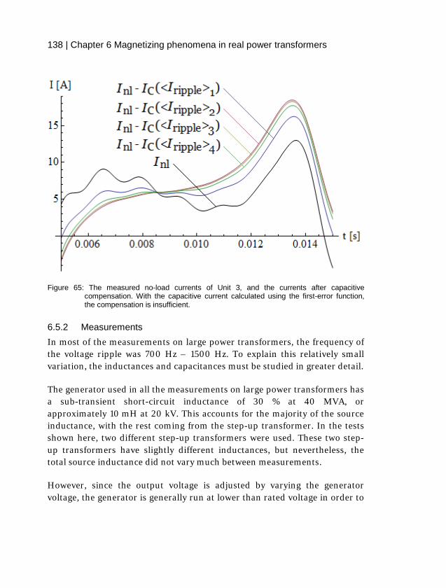
138 | Chapter 6 Magnetizing phenomena in real power transformers
Figure 65: The measured no-load currents of Unit 3, and the currents after capacitive compensation. With the capacitive current calculated using the first-error function, the compensation is insufficient.
6.5.2 Measurements In most of the measurements on large power transformers, the frequency of the voltage ripple was 700 Hz – 1500 Hz. To explain this relatively small variation, the inductances and capacitances must be studied in greater detail.
The generator used in all the measurements on large power transformers has a sub-transient short-circuit inductance of 30 % at 40 MVA, or approximately 10 mH at 20 kV. This accounts for the majority of the source inductance, with the rest coming from the step-up transformer. In the tests shown here, two different step-up transformers were used. These two step-up transformers have slightly different inductances, but nevertheless, the total source inductance did not vary much between measurements.
However, since the output voltage is adjusted by varying the generator voltage, the generator is generally run at lower than rated voltage in order to

6.5 Capacitive current and resonance | 139
allow overmagnetization of the tested transformer. IEC and IEEE standards stipulate that the no-load test should be performed at up to 110 % of the rated voltage. Additionally, keeping a margin means that the generator is not operating at its limit, and is thus able to deliver a more consistent voltage. The conversion ratio 𝑛𝑛SUT of the step-up transformer in (59) is therefore lower than the ratio of the rated voltages of the generator and the TUT. Accordingly, the impedance seen by the transformer under test is higher than would be expected from simply looking at the voltage. Since it does not influence the no-load loss measurement, the exact conversion ratio used in a specific test is usually not documented. This makes it difficult to estimate the exact inductance.
The effective capacitances were approximated using the method described on page 134, but the primary side capacitances could not be measured directly. With Cp thus omitted, the calculated resonance frequency is higher than the measured.
With only the effective capacitances inserted into the equation, the transformers fall into two groups. The transformers in the first group all have calculated resonance frequencies on the order of 1500-2000 Hz, while the second group has calculated resonance frequencies on the order of 2500-3000 Hz. Interestingly, the two groups were measured with different step-up transformers. This is probably related to how the step-up transformers are connected. To make the step-up transformers as versatile as possible, they can be reconnected in a large number of different ways. The impedances are therefore transformed differently, thus giving different calculated resonance frequencies. This is, however, an entirely artificial distinction caused by trying to calculate the resonance frequency without knowing the exact circuit impedances. When the resonance frequencies are measured, and not calculated, they do not appear to depend on the step-up transformer. This once again shows the importance of accurately representing the circuit impedances.

140 | Chapter 6 Magnetizing phenomena in real power transformers
6.5.3 Simulations The circuit model shown in Figure 61 on page 131 was used in the TTM to simulate the capacitive resonance. The results were then compared to measurement results in order to verify the theory outlined in section 6.5. To simplify the model, the step-up transformer was not modelled. Instead, the source voltage Ug and the source impedances were transformed up to the rated voltage.
The TTM is capable of simulating the resonance, as seen in Figure 66. This simulation used the measured 𝐶𝐶eff = 0.69 µF, and the approximated 𝐶𝐶𝑝𝑝 = 1.5 µF. Additionally, a shunt resistance had to be added to the source in order to model the losses of the generator and of the step up transformer. This resistance, which is on the order of 1.5 kΩ, serves to damp the oscillation.
Figure 66: Measured and simulated hysteresis curve (B-I) of unit 2 with capacitance included.
The additional impedances also improve the agreement with measured values. In this case, Δ𝐼𝐼rms decreases from 17 % to 14 %. However, this

6.5 Capacitive current and resonance | 141
modeling of the source is oversimplified. The real losses are divided among load and no-load losses. Modeling them using a single resistance is therefore not entirely correct. Nevertheless, it serves to demonstrate that including the electrical circuit is critical in order to achieve accurate simulation results (see also chapter 5.7.6). Further work should focus on measuring these source impedances so that they may be included in the simulation.
When the resonance is included, the simulation must be run with a shorter time step. This is because the time stepping introduces an artificial damping. With the non-linear TTM implemented, Simulink cannot treat inductances and capacitances using the built-in functions. If an inductance or capacitance is connected to one of the controlled current sources used in the TTM, the simulation tends to crash. To get around this, inductances and capacitances must instead be constructed as combinations of resistances and current- or voltage-sources (Figure 67).
Figure 67: Equivalent models of a capacitance (a) and an inductance (b). Since the TTM is non-linear, inductances and capacitances cannot be solved analytically. Instead they are based on the differences between one time-step and the next.

142 | Chapter 6 Magnetizing phenomena in real power transformers
The inductances and capacitances are therefore defined by the relationships
𝑈𝑈L = 𝐿𝐿Δ𝐼𝐼Δ𝜕𝜕
, (65)
𝐼𝐼C = 𝐶𝐶Δ𝑈𝑈Δ𝜕𝜕
(66)
This approximation of the derivative is good provided that the time step Δ𝜕𝜕 is short. However, it gives the average during the time step, and therefore is really valid for the time instant 𝜕𝜕 − Δ𝑡𝑡
2, and not for the time instant t. This
introduces a phase shift of 𝜔𝜔Δ𝑡𝑡2
rad. This, in turn, corresponds to equivalent
resistances of:
𝑅𝑅equiv,L = 𝜔𝜔𝐿𝐿
tan�π2−𝜔𝜔Δ𝑡𝑡2 �
, (67)
𝑅𝑅equiv,C = 1
ωC tan�π2−𝜔𝜔Δ𝑡𝑡2 �
. (68)
An RLC circuit has a damping coefficient ζ defined by
𝜁𝜁 =𝑅𝑅2�𝐶𝐶𝐿𝐿
, (69)
At the resonance frequency, the inductive impedance is equal to the capacitive impedance, and thus (67) and (68) give 𝑅𝑅equiv,L = 𝑅𝑅equiv,C. With 𝑅𝑅 = 𝑅𝑅equiv,L + 𝑅𝑅equiv,C, the damping becomes
𝜁𝜁 =
1
tan �π2 −𝜔𝜔rΔ𝜕𝜕
2 � ,
(70)
This gives critical damping, 𝜁𝜁 = 1, for
Δ𝜕𝜕 =2 atan(1) − 𝜋𝜋
𝜔𝜔𝑟𝑟. (71)

6.5 Capacitive current and resonance | 143
When simulating a transformer with resonance, the time step must therefore be chosen much smaller than this. Figure 68 shows a simulation of Unit 2 using two different time-step lengths. For this unit, Δ𝜕𝜕 = 100 µs corresponds to 𝜁𝜁 ≈ 0.3. This quickly damps out the oscillations. If Δ𝜕𝜕 is decreased to 10 µs (𝜁𝜁 ≈ 0.03), the oscillation is accurately reproduced.
Figure 68: One half-period of the simulated no-load current of Unit 2. With a 10 µs time step, the resonance of the circuit is simulated accurately, but increasing the time step to 100 µs damps out much of the resonance.

144 | Chapter 6 Magnetizing phenomena in real power transformers

7 Core diagnostics
The previous chapters of this thesis have shown that, with the appropriate correction techniques, the magnetizing currents of large power transformers are predictable and consistent. This means that any defect in the core that leads to a change in the magnetization current can be detected. Additionally, different types of core defects and different defect locations lead to different changes in the magnetization current. Thus, by studying the magnetizing current, or the no-load current, the defect can also be diagnosed.
This chapter outlines this diagnostic method and how different types of faults can be distinguished.
7.1 Distinguishing different types of faults Previous work within this project [6] has shown that different types of faults give different characteristic changes in the no-load current of single-phase transformers. The same principles apply to three-phase transformers as well. The interaction between the phases of a three-phase transformer makes the analysis more difficult, and there is more variation in how three-phase transformers are constructed. On the other hand, these facts also make three-phase currents more sensitive, and it is therefore possible to extract more information about a core defect.
In this section, the three simplest faults will be discussed. These faults are air gaps in the magnetic circuit, and circulating currents either around the whole core cross-section, or around a part of the cross-section.
Using only visual inspection of the magnetizing currents, it can be difficult to detect changes due to faults or defects. The plots in this chapter therefore show the difference between the currents in the healthy unit and the currents in the unit with the fault. However, the flux density at which the fault signature appears is crucial to the analysis of the fault. Therefore, the current difference is plotted as a function of the flux density (or, strictly speaking, the integral of the voltage). In the case of a three-phase unit energized from a
146 | Chapter 7 Core diagnostics
delta winding, the winding currents can usually not be directly measured. The measured currents are therefore the currents into the transformer terminals. Similarly, the voltages used to calculate the “flux density” are the line-to-ground voltages.
7.1.1 Partial air gaps Actual air gaps that cover the whole core cross-section are very rare in large power transformers. Cores are never27 constructed with this type of air gap, and for one to appear in in service would likely mean that the yoke has separated from the limbs. While this is possible as a result of a short circuit, it would lead to the total destruction of the transformer. Diagnostics would not be necessary.
Partial air gaps, where only a few laminations or core packages are affected, are more plausible. This could happen, for example, during manufacturing or due to some minor damage during transport or operation. A type of virtual air gap could also appear if the magnetic properties of some laminates were deteriorated. The permeability of those laminates could then decrease in a similar way as if there were an actual air gap.
When there is an air gap in a part of the core cross-section, this leads to flux being pushed into the surrounding areas, thus increasing the saturation. This can happen because of mechanical damage to the core, or because of an area of low permeability. However, it also occurs due to the air gaps in the core joints, and it is perhaps easiest explained in this context.
The simplest example of a partial air gap is in a single-step-lap joint of the type found in some reactors and in simpler transformers. In a single-step-lap joint, the flux will primarily pass through the gap bridge shown in Figure 69, but as the gap bridge saturates, its reluctance rapidly approaches that of the
27 There are cases where air gaps can be put in cores, either to increase the short-circuit impedance, or to change the remanence characteristics of the transformer. This is not done with large power transformers, however, and will be ignored here.

7.1 Distinguishing different types of faults | 147
actual air gap. When this happens, the total reluctance of the gap and the gap bridge approaches that of just an air gap.
Figure 69: Cross section view of a single-step-lap joint. The grey areas show the gap bridges, which will be overmagnetized by the flux being diverted from the air gap.
The actual flux profile under these conditions becomes very complex, as described in [77], [78], and for accurate results, calculations must be performed considering two- or preferably three-dimensional flux. However, the gap region is quite small compared to the total volume of the core, and the effect of the gap region on the total magnetization current is therefore small. This means that a joint can be described in a lumped element model with just a few reluctance elements describing the entire joint.
When simulating this type of joint, there are at least four options:
1. The joint can be simulated with full 2D or 3D geometries. This gives an exact representation of the joint, but the simulation is very time-consuming, particularly if hysteresis and the electrical circuit need to be considered. This option has not been pursued in this paper.
2. The core can be split into two parallel reluctances, and an air gap inserted into one of them (Figure 70 a). This effectively makes the whole core into one single step-lap joint. For this approach to work, the out-of-plane flux must be modeled using an additional reluctance element. This
148 | Chapter 7 Core diagnostics
element is then an average of the out-of-plane component of the flux in the entire core.
3. The gap bridge can be modeled as a non-linear element with length and cross-section equal to those of the gap bridge (Figure 70 b). This element is then put in parallel with an air reluctance corresponding to the air gap. This ignores the out-of-plane flux, and can be implemented in models with only a single flux path. However, the flux in the non-linear element becomes very high, and this can become an issue for the hysteresis model.
4. The joint can be simulated as a conditional virtual air gap [41]. The length of this virtual air gap is equal to the length of the actual air gap if the core flux density is above a certain critical value 𝐵𝐵crit , and otherwise it is zero (i.e. the reluctance is short-circuited). In [41], the critical flux density is assumed to be the flux density when the gap bridge is fully saturated while the flux density in the air gap is zero. This gives
𝐵𝐵𝑒𝑒𝑟𝑟𝑖𝑖𝑡𝑡 =𝑁𝑁SL
𝑁𝑁SL + 1𝐵𝐵𝑆𝑆 , (72)
where NSL is the number of steps in the step-lap joint, and BS is the saturation flux density. In a single-step-lap joint, NSL =1, and the critical flux density is approximately equal to 1 T. This method, shown in Figure 70 c) is the easiest to implement, but it neglects the gradual saturation of the gap bridge. For this reason, it gives a more abrupt transition into saturation.
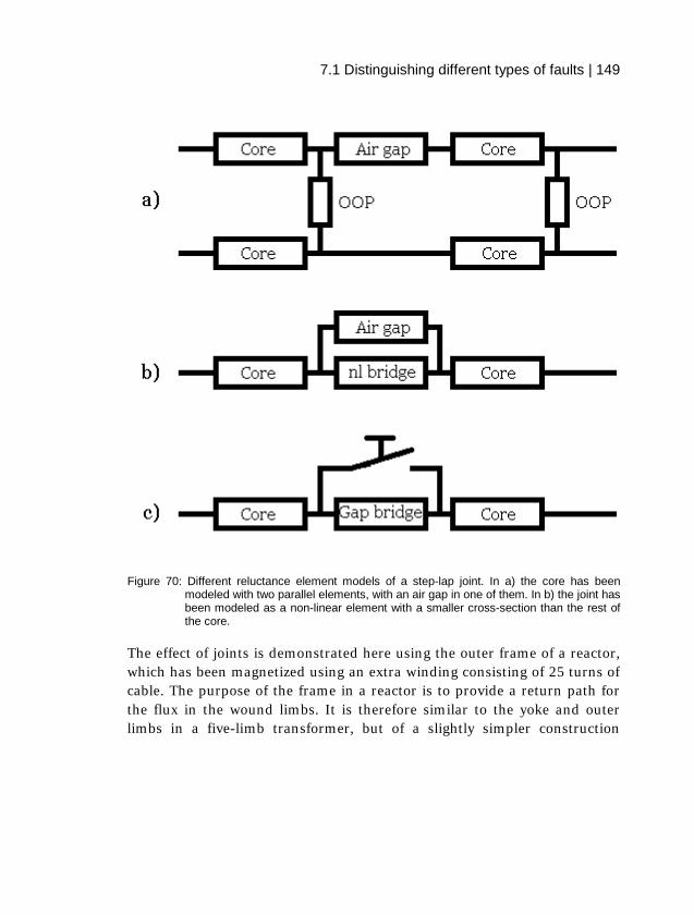
7.1 Distinguishing different types of faults | 149
Figure 70: Different reluctance element models of a step-lap joint. In a) the core has been modeled with two parallel elements, with an air gap in one of them. In b) the joint has been modeled as a non-linear element with a smaller cross-section than the rest of the core.
The effect of joints is demonstrated here using the outer frame of a reactor, which has been magnetized using an extra winding consisting of 25 turns of cable. The purpose of the frame in a reactor is to provide a return path for the flux in the wound limbs. It is therefore similar to the yoke and outer limbs in a five-limb transformer, but of a slightly simpler construction

150 | Chapter 7 Core diagnostics
(Figure 71). All joints are single step lap joints, and the joints in the yoke are not T-joints as in transformers, but simple straight joints28.
Figure 71: Schematic of a reactor frame. During this test, the wound limbs were not yet installed, and the voltage was supplied using a coil placed around one side limb. In addition to the corners, the reactor frame also has joints in the yoke (joints shown in blue).
Figure 72 shows the effect of this single step lap joint. Once the flux density reaches 𝐵𝐵𝑠𝑠/2, the gap bridge is fully saturated, and the flux is forced through the higher reluctance air gap.
28 This means that the flux in the wound limbs enters the yoke perpendicular to the rolling direction. This increases the total reluctance, but that is not an issue in a reactor, since the reluctance is much higher than in a transformer to begin with.

7.1 Distinguishing different types of faults | 151
Figure 72: No-load current of a reactor frame. The air gaps in the joints cause a sudden increase in the magnetizing field at a flux density of approximately 1 T.
In power transformers with multiple-step-lap joints, the gap bridge requires a higher flux density before it saturates. In a core with a six-step step-lap, the saturation will start to occur at a core flux density of approximately 1.74 T, and since the entire core is already approaching saturation, the effect will be much less noticeable.
If the partial air gap is due to a fault or defect in the core, the expected signature in the no-load current is the same. The critical flux density shows the fraction of the core that is involved in the air gap, and the increase in magnetizing field shows the length of the air gap (or strictly speaking the increase in reluctance due to the air gap).

152 | Chapter 7 Core diagnostics
Figure 73: If the transformer is delta-connected, each terminal current is the sum of the currents in two limbs. This also means that a fault signature shows up in two of the measured currents. For example, a fault in limb 1 will affect the currents in both phase a and in phase b.
In a three-phase transformer, the signature is not as straightforward as in the single-phase case shown earlier. This is partly due to the interaction between the phases, but it is also due simply to the fact that some of the interesting quantities are not measurable. For example, in a delta-connected winding, a fault in limb 1 will appear in both phase a and in phase b, since both of them contain part of the current in limb 1 (Figure 73). Also, the calculated “flux density” is not the flux density in the limbs.
Nevertheless, there are clear similarities to the single-phase case. Figure 75 shows the difference between two simulations of Unit 11. First, the healthy transformer was simulated. Then a 1 mm long air gap was introduced in the T-joint of one of the outer wound limbs (Figure 74). This air gap covered half the core cross-section, and was modelled using the method shown in Figure 70 a.

7.1 Distinguishing different types of faults | 153
Figure 74: Connection (blue) and fault location (red) during simulation of an air gap in Unit 11.
The air gap leads to increased current peaks in all phases. Interestingly, there is a low-frequency (25 Hz) oscillation that makes the peak currents in the simulation with the air gap alternatingly higher and lower than those in the simulation without the air gap. This can be seen as the difference plot being symmetric. For example, the air gap first gives a higher peak current in phase b (green in the figure). This gives the peaks in the first and third quadrants. Then, in the next period, the current in phase b is actually lower with the air gap than without it. The peaks are then in the second and fourth quadrants. During this period, the air gap gives increased current peaks in the other two phases. This gives the impression that the fault current moves back and forth between the phases every second period. The simulation results suggest that it is an effect of the return limbs. The air gap causes the return limbs to alternatingly receive a higher flux.
This phenomenon needs to be studied further. It could be just an artifact of the simulation. On the other hand, if the resonance exists even in real transformer, it could be useful for diagnostics. The phenomenon could also be related to the fact that the currents in a three-phase transformer are all different. This was described briefly in chapter 6.1, and is of practical use for diagnostics, as will be discussed further in chapter 7.3.

154 | Chapter 7 Core diagnostics
Figure 75: Simulated differences in no-load currents from an air gap in one of the T-joints in Unit 11.Unlike single-phase simulations, which only have peaks in the first and third quadrants, this simulation has peaks in all quadrants and in all currents (except possibly phase a (red) in the first quadrant, and phase c (blue) in the third quadrant).
The fault signature appears at the magnetization peak, where the simulation gives the largest error, and where a small difference in the supply voltage can give a large difference in the measured result. For this reason, it may be difficult to detect this type of fault. However, there is no appreciable increase of the losses in this case, whereas Δ𝐼𝐼 reaches more than 10 %. Thus, there is an amplification effect, and it should be possible to detect air gaps before they cause problems for the transformer.
7.1.2 Circulating currents around the whole core cross-section When there is a path for circulating currents around the whole core cross-section, this will act as an additional resistive load on the affected phase. The circulating current path can be caused either by a problem in a winding, or in the core.
7.1 Distinguishing different types of faults | 155
In the case of a circulating current in a winding, the problem is usually caused by a mistake during manufacturing, and it will have a very obvious effect on the no-load losses. The fault resistance is low, and with the full turn voltage driving the fault current, the additional losses can reach several tens of kilowatts.
The less obvious, and therefore more relevant, case is when the circulating current runs in the core. This can, for instance, be the case if the interlaminar resistance is low. If the insulating layer between core laminations is damaged or insufficient, or if the edges of the laminations have burrs, which provide low-resistance current paths, then a circulating current can flow in the core itself [79]–[81]. In this case, the resistance is higher, and the currents consequently lower, than when the circulating current flows in a winding. The interlaminar resistance is routinely measured on new transformers, and the resulting loss increase can be calculated analytically [82].
Regardless of the cause of the circulating current, the result is a purely resistive loss current, which is added to the nominal no-load current.
7.1.3 Circulating currents around part of the core cross-section In the previous chapter, a fault that affected the whole core cross-section was studied. However, in many cases, there are physical limitations to the fault. For example, burrs might affect only a certain core packet, poor insulation might affect only one roll of steel, or the circulating current might be limited by cooling ducts in the core. In such cases, the flux will be forced into different paths depending on the magnetization state of the core.
This behavior is similar in nature to that described when there is a partial air gap in the core, but it is more affected by the non-linearity of the material. When the flux density is low, it is advantageous for the flux to flow almost exclusively in the part of the core that does not have the fault. This will increase the flux density in this part, but since the flux density is low, this will only lead to a minor increase in the current and loss. As the flux density increases into the non-linear region, more and more flux will pass through

156 | Chapter 7 Core diagnostics
the fault and contribute to the circulating current there. This results in an increase of the no-load current at the knee of the magnetization curve.
Figure 76: The impact of a circulating current path depends on the position of the fault. A fault that covers the whole core cross-section (A) gives a different signature than one that only covers part of it (B, C). Also, if the fault is on the inner part of the core (B), the healthy flux path is longer than the path through the fault, and this gives a different signature than if the fault is on the outer part of the core (C) and the healthy flux path is shorter than the path through the fault.

7.1 Distinguishing different types of faults | 157
Since the path that the flux takes depends on the reluctance of the fault relative to the reluctance of the healthy part of the core, the fault signature will also vary depending on the position of the fault within the core (see Figure 76). This difference can be seen in Figure 77. When the fault is on the inside part of the core (B in Figure 76), the signature is more similar to the signature of a fault around the whole core cross-section. This is because it is more advantageous to have a shorter magnetic path, and thus a lower reluctance, even if the losses are higher. With the fault on the outside part (C) of the core, on the other hand, the healthy part of the core offers a path that is both shorter and free of the resistive losses of the fault. In this case, the no-load current gets a very marked peak just below the knee, i.e. when saturation starts becoming a factor.
Figure 77: Simulation of a single-phase transformer with a fault affecting the half of the core cross-section. The signature is different depending on whether the fault is in the outer or inner part of the core.
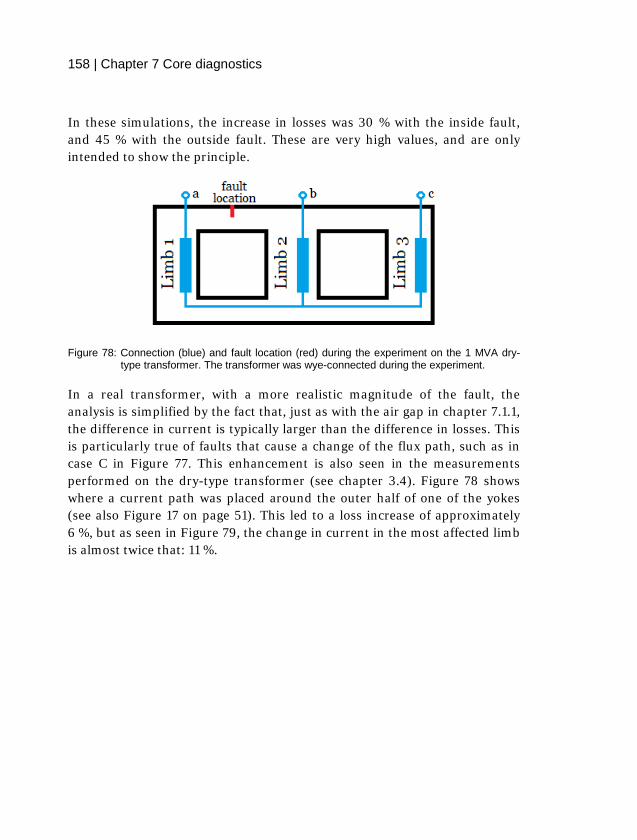
158 | Chapter 7 Core diagnostics
In these simulations, the increase in losses was 30 % with the inside fault, and 45 % with the outside fault. These are very high values, and are only intended to show the principle.
Figure 78: Connection (blue) and fault location (red) during the experiment on the 1 MVA dry-type transformer. The transformer was wye-connected during the experiment.
In a real transformer, with a more realistic magnitude of the fault, the analysis is simplified by the fact that, just as with the air gap in chapter 7.1.1, the difference in current is typically larger than the difference in losses. This is particularly true of faults that cause a change of the flux path, such as in case C in Figure 77. This enhancement is also seen in the measurements performed on the dry-type transformer (see chapter 3.4). Figure 78 shows where a current path was placed around the outer half of one of the yokes (see also Figure 17 on page 51). This led to a loss increase of approximately 6 %, but as seen in Figure 79, the change in current in the most affected limb is almost twice that: 11 %.

7.1 Distinguishing different types of faults | 159
Figure 79: Current differences in the 1 MVA transformer from a current path around half the cross section. The current path was placed close to phase a (red). Since the exact dimensions of the transformer are not known, the flux density is an approximation.
Just as in the single-phase case (Figure 77), the loss increase occurs in the affected limb just below the knee (at approx. 1 T). That it occurs at a slightly lower flux density than in the single-phase case has to do with the lower steel quality in the 1 MVA unit, and more importantly, that the cross-section of the core of the 1 MVA transformer is unknown. The flux density is therefore an approximation, and it may have been underestimated.
In accordance with Kirchhoff’s current law, the total current into the transformer must be zero. The extra current in phase a due to the fault must therefore be drawn from the other phases. Magnetically, it is more favorable to draw it from the other outer limb (blue). The current and loss in the middle limb (green) is therefore practically unaffected by the fault. Thus, the behavior of all three phases is characteristic of this particular fault type and of this particular fault location.

160 | Chapter 7 Core diagnostics
Figure 80: Connection (blue) and fault location (red) during the simulation of Unit 11.
Simulations confirm these results, and allow them to be extended to other units and to other faults and fault locations. As an example, Unit 11 was simulated with a current path around one of the return limbs. The current path was placed around half the core cross-section on the part of the limb closest to the core window (Figure 80). The resistance of the current path was 2 Ω, and the resulting loss increase was 5 %. As shown in Figure 81, the increase of the currents was almost 20 %.

7.2 Diagnosing a core | 161
Figure 81: Simulated current differences in Unit 11 from a current path around part of one return limb.
Unit 11 is delta-connected, has five limbs, and the fault is in a different location than in the 1 MVA unit. The fault signature is therefore different from in Figure 79. Still, there are also enough similarities to make diagnostics possible. It is clear that it is the same general type of fault in both cases.
It should be noted that in real transformers, it is far more likely to have a fault that affects one core package (see chapter 2.3.7) than one that affects the outer or inner part of the core as shown here. This is because burrs, which are the most common cause of circulating currents, can only occur at the edges of the sheets. The principle that the location of the fault determines the fault signature remains the same, however.
7.2 Diagnosing a core As has been shown, it is possible to diagnose a transformer by the changes that a fault causes in the no-load current. However, a measurement of the

162 | Chapter 7 Core diagnostics
no-load current of the transformer in a verifiably healthy condition is not always available. In these cases, it becomes necessary to compare the transformer to something else.
This thesis presents four such methods:
1. The no-load currents can be compared to those of a similar unit.
2. The no-load current can be compared to a simulation.
3. The phases can be compared to each other in a three-phase transformer.
4. The no-load currents can be compared at different voltage (flux density) levels.
Options 1 and 2 have been demonstrated earlier in this thesis, and options 3 and 4 will be discussed in the following sections.
7.3 Three-phase symmetry As discussed in Chapter 6.1, the no-load current of a three-phase transformer depends not just on the core, but also on the electrical circuit.
Since the imbalance is dependent on the phase order, the no-load current in a certain phase will also be different depending on whether that phase is magnetized before or after the middle phase. However, as long as there is no physical (or magnetic) difference between the two outer limbs, this difference depends only on the order in which the phases are magnetized. If the phase order is reversed, the currents should change between the two outer limbs, but otherwise be unchanged.
This can be used for diagnostic purposes, since most power transformers are designed to be physically and magnetically symmetric. By making two measurements with different phase orders, any difference between the two measurements must be due to a physical or magnetic asymmetry.
This principle is demonstrated in Figure 82. Measurements were performed on Unit 16 during no-load testing. After the test, the phase order was

7.3 Three-phase symmetry | 163
reversed such that the feeding cables on terminals a and b were switched. The order in which the limbs were magnetized was thus reversed. The difference in currents between the two phase orders was then plotted.
The behavior in Figure 82 shows that one of the limbs has a significantly higher peak H-field than the other, but apart from this, the limbs are quite similar. In this case, the higher peak current is caused by remanence in the core (see Chapter 6.3). The transformer had been run at 110 % for almost 30 minutes before the measurements, but there was still significant remanence. It is therefore not possible to see any other asymmetries in this unit.
Figure 82: Differences in currents between the two phase orders in Unit16. This particular behavior is indicative of a DC bias.
To see how this can be used to detect a core fault, Unit 11 was simulated with a current path around part of one of the return limbs. The simulation was then repeated with the phase order reversed. The reversal was achieved by switching the connections on terminals b and c. The difference between the two phase-orders are shown in Figure 83. As seen in the figure, the

164 | Chapter 7 Core diagnostics
difference between the two phase orders is quite dramatic even for a relatively small fault (the increase in no-load losses due to the fault was 5.5 %).
Figure 83: Simulated differences between the two phase orders with a current path on the return limb next to limb 3.
The fault shown here is almost the same as that used for Figure 81. The only difference is that it is located on the opposite side of the transformer, on the return limb next to limb 3 (i.e. on the right hand side of the transformer in Figure 80 on page 160). The reason for this is to illustrate a limitation in this method. In a delta-connected transformer, there is always one terminal (terminal a) that is connected to the two outer limbs. No matter how the phases are ordered, the current in terminal a is the sum of the two outer phases. The diagnostic method relies on the difference between the outer limbs and the middle limb. Thus, any fault that mainly affects the current in terminal a can not be detected.
Also, regardless of whether the transformer is delta- or wye-connected, the method can only detect asymmetric faults. That is: faults that are physically
7.4 Comparison between voltage levels | 165
located on one side of the transformer. It will therefore be difficult to resolve faults located in the middle limb.
On the other hand, for those faults that can be detected, the resolution is high. As long as the remanence can be eliminated, the only other major source of error is how closely the voltage can be reproduced from measurement to measurement. Since the transformer is being compared to itself, it is reasonable to expect that the difference in currents between the phase-orders should, for an ideal (i.e. healthy) transformer, be small. Some difference is unavoidable, due to manufacturing tolerances, measurement inaccuracy, variations in the source voltage, etc. However, this “noise” should be on the order of 5 % - 10 % of the rms currents. On the other hand, differences due to a fault or defect are expected to be far larger. For example, Figure 83 shows differences of 20 % - 30 %, even for a relatively modest fault. This should be clearly distinguishable from the noise.
7.4 Comparison between voltage levels Since the characteristic signature of a fault is flux dependent, the fault could be detected and diagnosed by performing measurement at different voltage (or flux density) levels. Apart from the characteristic signatures appearing at different flux densities, they also depend differently on the rate of change of the flux. For example, a circulating current around the core is proportional to dB/dt, while the magnetizing field in an air gap is proportional to B. Changing the peak flux density, and thus dB/dt, could therefore yield additional information.
This method is not particularly sensitive since the achievable change in dB/dt is rather small. The method is therefore best seen as a last resort, or as a means of verifying a simulation.

166 | Chapter 7 Core diagnostics

8 Further work
There is room for further improvement before the method can be developed into a practically useful diagnostic tool. This chapter describes this work, both on the diagnostic method itself and on the simulation model. Additionally, some other applications for the simulation model, beyond the scope of this thesis, are described.
8.1 Development of a diagnostic tool The diagnostic method described here needs to be developed into a fully functional tool. To accomplish this, a larger number of transformers need to be tested. This work is ongoing, and will lead to a better understanding of the normal magnetizing current phenomena in healthy units. It is also important to find and diagnose units with some type of core defect. Units with core problems are few and difficult to find, but these measurements are vital to verifying the diagnostic method.
There are also practical concerns before the tool can be implemented. For instance, it should be usable not only in a transformer factory or repair workshop, but also in the field. In a transformer substation, the grid can be used to supply the voltage, and there are usually voltage transformers available for monitoring or protection purposes. The currents, on the other hand, may be difficult to measure. If there are current transformers for monitoring, they are usually dimensioned for the load currents, and therefore do not have the sensitivity required to measure no-load currents. The current probes therefore have to be brought specifically for the core diagnostic measurement. It may be difficult to find suitable current probes that are accurate, mobile, and still usable at full line voltages.
This type of field measurement has been attempted within this project [6]. This measurement demonstrated that diagnostics are, in principle, possible even in the field. However, it also illustrated that the practical implementation still requires work. The current probes used during the measurement were either not adequately shielded, leading to cross-talk with

168 | Chapter 8 Further work
the line voltages, or they were not sensitive enough. For the diagnostic tool to be considered fully usable, these issues have to be addressed.
This mainly involves evaluating different current measurement technologies. Rogowski coils are a promising solution since they can usually be made large enough to place around the bushings, and thus do not require much downtime for installation. In the measurement described in [6], Rogowski coils were used, and in that case, the transformer was back online within two hours of initiating the shut-down. With practice, this time could be further reduced29. The Rogowski coils must, however, be shielded in order to avoid cross-talk. The shielding influences the frequency characteristics [83]. This effect, and any possible effect of the bushings on the measurement, must be investigated before implementation.
If the onboard current transformers are used instead, these must be calibrated especially for the no-load current measurement. In most large power transformers, the no-load current is less than a percent of the currents that the onboard current transformers are designed to measure. At these low currents, the magnetization current of the current transformer itself is not negligible. This makes the current transformer non-linear. This can be calibrated for, but doing so requires work and reduces the accuracy of the measurement.
The advantage of performing this calibration is that it would make it possible to perform diagnostics completely without downtime. If there are current transformers on both the primary and secondary windings, the no-load current can be calculated from the difference between these. The no-load current diagnostics could therefore be performed even with the transformer under load.
29 Rogowski coils could, in theory, be installed entirely without disconnecting the transformer. However, form a safety perspective, a short disconnection is probably preferable to working on live electrical equipment.

8.2 Improvement of the simulation method | 169
However, not all power transformers are equipped with onboard current transformers. This, combined with the easier handling, make Rogowski coils easier to implement.
8.2 Improvement of the simulation method As described in chapters 5.7.7 and 5.8.3, the simulation method is rather accurate, but requires further refinement in order to be universally applicable. Further work is mainly required in four areas: the program implementation, the modeling of the source impedances, the amount of detail in the magnetic circuit, and the hysteresis model.
8.2.1 The program implementation The present implementation in MATLAB and Simulink limits the number of non-linear elements that can be used. This has to do both with the simulation time and the time required to compile the program.
The time and memory required to compile the program increases quickly when the number of windings or non-linear elements is increased. With the standard desktop computer (8 GB RAM) used for this work, it was impossible to compile circuits with more than a hundred winding elements. While it might be possible to find a workaround, it is probably faster to convert the program to a different programing language. This could either be done by a transpiler, which automatically converts the program to a faster language (e.g. Fortran, C++, or an assembly language). Alternately, it could be done by converting the simulation into a language that is specifically built for simulating large systems (e.g. EMTP).
Another programing language could also be more optimal for the simulation. The advantage of Simulink is that the graphical interface makes it easy to build and overview complex systems. Also, the vast library of ready-made functions makes it easy to build models from scratch. With the TTM, however, the main part of the program has to be custom built anyway, and it has to be written without using the graphical interface. This negates the main advantages of using Simulink, and it might be better to switch to a programming language that is better suited to the task.

170 | Chapter 8 Further work
In terms of simulation time, however, the best improvement is probably just optimization of the code. The code, in its present form, is very computation-heavy. The simulation time could be significantly decreased by implementing a reluctance network solver that does not require inversion of large matrices.
The main bottleneck in terms of speed is solving the matrix equation 𝚫𝚫𝚽𝚽 = 𝓟𝓟Δ𝚫𝚫𝓕𝓕. In the described program, this is done using the built-in MATLAB function “mldivide()” (or “\”). For a square matrix such as 𝓟𝓟Δ, this is similar to inverting the matrix. While Mathsworks30 claims that the function is more robust compared to a matrix inversion, it is still computationally demanding. Though this is acceptable for small systems, for a larger number of reluctance elements, the algorithm becomes very slow. This is especially true when there is a large number of winding elements since the matrix equation, albeit slightly simplified, must be solved once per winding element in order to get 𝒀𝒀Δ.
In the field of power system engineering, there are faster algorithms for a similar problem. When modelling a large power grid, the bus admittance matrix, which is the electrical analog of 𝓟𝓟Δ, can frequently have thousands of elements. To deal with this, there are algorithms for converting between the bus admittance and the bus impedance matrices [84]. Then, the matrix equation can be solved through matrix multiplication rather than matrix inversion. The same principle could possibly be used in the TTM to find the inverse of 𝓟𝓟Δ. As this has not been done, it is, however, unclear how large the gain in speed would be.
Many of the elements of both 𝓟𝓟Δ and 𝒀𝒀Δ are zero, and the computation time could therefore be reduced by using a sparse matrix formulation. However, while MATLAB supports sparse matrices, Simulink does not. This makes them difficult to implement, and the possible gains were not deemed sufficient to merit the extra work. It could be something to consider, however, if the algorithm were implemented in another programming language.
30 The company developing MATLAB.

8.2 Improvement of the simulation method | 171
8.2.2 Impedance modeling The source impedances are presently included in a very simplified manner. This means that the simulated voltage is different from the actual voltage in the transformer. The simulated magnetization behavior is therefore also different from the real magnetization behavior. For the most part, this could easily be implemented in the simulation. It only requires accurate data on the source circuit.
In many cases, this data is available in the form of product specifications or calibration protocols. However, the effective impedances in any particular measurement depend on exactly how the circuit is connected. This is often based on the experience and routines of the operators, and these might not be as well-documented. In further measurements, care should therefore be taken to document the exact setup used in each measurement.
Even if the source impedances are measured, some of them should, ideally, be modeled as non-linear. This is primarily the case with the generator and step-up transformer. The step-up transformer could easily be simulated in the same manner as the test object. Similarly, the generator could also be simulated by the TTM. A generator has a greater amount of transverse flux, and higher flux harmonics than a transformer does. The TTM is not optimized for these conditions, and the accuracy would be lower than in the transformer simulations demonstrated in this thesis. On the other hand, during no-load testing, the voltage drop in the generator is low. Therefore, any simulation error when simulating the generator has a low impact. Simulating the generator assembly with the same accuracy as the tested transformer is very time-consuming, however, and probably not worth the effort.
8.2.3 Magnetic circuit modeling Increasing the amount of detail in the magnetic circuit simulation can improve the results. The most easily implemented improvement in this area is to incorporate non-linear transverse and out-of-plane flux. The hysteresis curve in the transverse direction can be measured using a normal SST. The out-of-plane magnetization curve is more difficult to measure using standard

172 | Chapter 8 Further work
equipment, but since it is dominated by the air gap reluctance between the sheets, it should be possible to approximate as linear. Then, the corner joints could be modeled with additional elements. In addition to improving the simulations, this would also make it possible to model the building factor. The building factor, i.e. the difference in losses between the core steel and the finished core, is generally attributed to the flux behavior in the joints.
If the transverse hysteresis curve is measured, the main obstacle to improving the magnetic circuit model is the simulation time. Thus, if the model can be optimized (or run on a more powerful computer), the accuracy of the results can also be improved.
8.2.4 The hysteresis model The hysteresis model used here is only an approximation. It gives reasonably good results with only a few inputs, i.e. one static curve and one dynamic curve. While this simplicity is desirable from an engineering point of view, it is does leave room for improvement when it comes to accuracy.
The problem with the static curve is mainly in the representation of small minor loops, and particularly those with high-flux-density reversal points. This leads to errors for flux with a high harmonic content. To some extent, the problem could be solved by introducing a weighting factor in the gate model. This would give more realistic minor loops. On the other hand, it would make the model more complicated without making it more physically correct. A better option is therefore to switch to a more advanced model. For example, the congruency-based model described in [61] could fairly easily be implemented. This requires measuring a larger number of first-order reversal curves, but would give a more correct description of minor loops.
The main obstacle to this is the difficulty of measuring FORCs with commercially available equipment. SST are usually primarily designed to measure the dynamic losses of the steel. Measurement of FORCs is not prioritized. It might, however, be possible to measure static hysteresis loops, as has been done in this thesis. For high flux-density reversal points, the

8.3 Further applications | 173
falling branch of the static loop is very close to being a FORC. This is also the region in which the gate model struggles. By using only a small number of high-reversal-point static loops as FORCs, it might be possible to arrive at an option in-between the gate model and the congruency-based model. This could make it possible to achieve high accuracy without requiring specialized equipment.
The modeling error in the dynamic hysteresis is mainly associated with the excess eddy current field. Improving this model would require performing a large number of measurements at varying frequency and flux density. Then, it would be possible to either calculate the excess eddy current parameters 𝑉𝑉0 and 𝑛𝑛0, or to make an interpolation of the excess eddy field directly from the measurements. It should be noted, however, that the magnetizing frequencies and flux densities in power transformers do not vary much from unit to unit. Therefore, the error from the modeling of the excess eddy current field is likely small compared to the other error sources mentioned here. If the simulation is generalized to other electrical machines, however, the model should be improved as described here.
8.3 Further applications Improving the simulation method benefits not only the core diagnostics described here, but also makes it possible to study other electromagnetic phenomena in transformers. For example, ferroresonance, a phenomenon that frequently causes failures in voltage transformers, is similar to the capacitive resonance described in chapter 6.5, and could be simulated in a similar manner [85], [86].
The simulation method could also be used to predict inrush [72], [87] or the effects of geomagnetically induced currents (GIC) [88]–[90]. With these types of high-saturation phenomena, hysteresis is often neglected. At the same time, however, there is a concern that the core losses could become dangerously high, particularly during a GIC event. It might therefore be interesting to include hysteresis in the simulation. There are also indications that the hysteresis might affect the currents themselves [91].

174 | Chapter 8 Further work
With hysteresis implemented in the way described here, the method is not optimized for these types of high-saturation phenomena. This leads to some stability issues. Also, the method has not been verified for extremely high flux densities (>1.95 T). However, the method was first designed exactly for GIC simulation, and further development could extend the useful range.
To accomplish this, the time-step must adapt and become shorter for high flux density. Additionally, a check would be necessary to prevent the magnetization curve from straying outside the major loop. Even with a short time-step, this can easily happen at high flux density. This then leads to negative values in the gate model, and the simulation tends to crash. Such a check is fairly simple to implement, however, and would allow simulation of GIC and inrush with the same accuracy as for the no-load current.
In addition to modeling existing transformers, the simulation method could also be used to predict the performance of new core designs. This could then allow a manufacturer to design cores that are optimized for a particular purpose. As mentioned earlier, there have been attempts to improve core performance by, for example, changing the joint angles [44], or by mixing different steel grades [40]. These, and other, examples show that deviating from the conventional design could potentially give better cores, but requires rigorous testing. For that, computer simulations are a cost-effective solution.

9 Conclusions
This thesis has demonstrated that it is possible to diagnose the core of a power transformer by studying the no-load current. Different types of core faults and defects lead to different characteristic changes in the no-load current. These changes are typically larger than the corresponding changes in the no-load losses, and no-load current diagnostics are thus more sensitive than no-load loss measurements.
In order to perform these diagnostics, the no-load currents must be compared to some ideal wave-form. This can come either from another similar unit that is known to be healthy, or from a simulation. For three-phase transformers, it is also possible to compare the phases to each other.
If a simulation is used, it must be accurate enough that the fault can be distinguished. One such simulation method has been demonstrated here. This method delivers sufficiently accurate results in some cases, but further work is necessary in order to make it universally reliable. Much of this work is to optimize the code. That way, the number of reluctance elements can be increased, thus also increasing the accuracy.
The choice of simulation method is not critical as long as the chosen method includes all relevant phenomena. The impact of neglecting certain effects has been described and quantified in this thesis. The results can thereby be generalized to any simulation method.
If a transformer is compared to another unit, there are techniques that must be applied in order to avoid certain obfuscating effects. To accomplish this, techniques have been described for compensating for the effects of capacitive currents and of resonance. Additionally, a method has been proposed for estimating the effective magnetic length of the core.
Finally, a method for comparing the phases of a three-phase transformer to each other has been demonstrated. This is not trivial, since the three phase currents are always different. However, as shown herein, these differences

176 | Chapter 9 Conclusions
are mainly due to electrical interactions. They can therefore be removed by changing the order in which the phases are magnetized. This method is not suitable for all applications, but when applicable, the resolution is high.
To summarize the thesis, it is worthwhile to return to the aim of the project: to develop a method for transformer core diagnostics. While some work remains regarding the practical implementation, this aim must be considered fulfilled. The no-load current is a sensitive and reliable indicator of the health of a transformer core. By studying it, an operator can detect and diagnose even small changes in the core.
The secondary aim, to make the method applicable on-line, requires further field testing. However, the principle has been proven, and the remaining work mainly involves selection and testing of the measurement equipment. The diagnostic method itself can be performed with little downtime, and with equipment that is available to most transformer manufacturers and operators.
Finally, the diagnostic method can also be used to study the details of the magnetization process of a large power transformer. While not explicitly stated as an aim at the outset of the project, this is useful for improving transformer cores in general. Accurate simulation methods make it possible to design and optimize new transformer cores. Accurate measurement methods make it possible to test these new designs and verify the improvements. Thus, the results of this thesis can be used not only to predict and pre-empt failures in the transformers of today, but also to improve the transformers of tomorrow.

References | 177
References
[1] ‘Large Power Transformers and the U.S. Electric Grid’, Infrastructure Security and Energy Restoration Office of Electricity Delivery and Energy Reliability U.S. Department of Energy, Apr. 2014.
[2] ‘State Electricity Profiles - Energy Information Administration’. [Online]. Available: https://www.eia.gov/electricity/state/. [Accessed: 19-May-2017].
[3] X. Zhang and E. Gockenbach, ‘Transformer Diagnostic and Assessment Methodology’, in Conference Record of the 2008 IEEE International Symposium on Electrical Insulation, 2008. ISEI 2008, 2008, pp. 128–131.
[4] B. S. Munir, J. J. Smit, and I. G. M. R. Rinaldi, ‘Diagnosing winding and core condition of power transformer by vibration signal analysis’, in 2012 International Conference on Condition Monitoring and Diagnosis (CMD), 2012, pp. 429–432.
[5] IEC 60076-1, ‘Power Transformers - Part 1: General’. 2011. [6] C. Carrander, On methods of measuring magnetic properties of power
transformers. Stockholm, Sweden: Kungliga Tekniska Högskolan, 2015.
[7] C. Carrander and G. Engdahl, ‘Magnetizing current measurements on full scale power transformers’, Int. J. Appl. Electromagn. Mech., vol. 48, no. 2,3, pp. 159–162, Jun. 2015.
[8] C. Carrander, S. A. Mousavi, and G. Engdahl, ‘An application of the time-step topological model for three-phase transformer no-load current calculation considering hysteresis’, J. Magn. Magn. Mater., vol. 423, pp. 241–244, Feb. 2017.
[9] C. Carrander and G. Engdahl, ‘A semi-empirical approximation of static hysteresis for high flux densities in highly grain-oriented silicon iron’, Joint European Magnetic Symposia, 2016.
[10] C. Carrander, ‘Power transformer core diagnostics using the no-load current’, presented at the 1&2DM2016, Tianjin, China, 2016.
[11] F. Fiorillo, ‘Measurements of magnetic materials’, Metrologia, vol. 47, no. 2, p. S114, Apr. 2010.
[12] W. Rave, R. Schäfer, and A. Hubert, ‘Quantitative observation of magnetic domains with the magneto-optical Kerr effect’, J. Magn. Magn. Mater., vol. 65, no. 1, pp. 7–14, Feb. 1987.
[13] R. D. Gomez, A. A. Adly, I. D. Mayergoyz, and E. R. Burke, ‘Magnetic force scanning tunneling microscopy: theory and experiment’, IEEE Trans. Magn., vol. 29, no. 6, pp. 2494–2499, Nov. 1993.

178 | References
[14] W. Gerlach and O. Stern, ‘Der experimentelle Nachweis der Richtungsquantelung im Magnetfeld’, Z. Für Phys., vol. 9, no. 1, pp. 349–352, Dec. 1922.
[15] B. D. Cullity and C. D. Graham, Introduction to Magnetic Materials. Hoboken, NJ, USA: John Wiley & Sons, Inc., 2008.
[16] N. Takahashi, M. Morishita, D. Miyagi, and M. Nakano, ‘Comparison of Magnetic Properties of Magnetic Materials at High Temperature’, IEEE Trans. Magn., vol. 47, no. 10, pp. 4352–4355, Oct. 2011.
[17] L. D. Landau and E. Lifshitz, ‘On the theory of the dispersion of magnetic permeability in ferromagnetic bodies’, Phys. Z. Sowjet., 1935. [Online]. Available: http://cds.cern.ch/record/437299. [Accessed: 10-Jan-2017].
[18] E. C. Stoner and E. P. Wohlfarth, ‘A Mechanism of Magnetic Hysteresis in Heterogeneous Alloys’, Philos. Trans. R. Soc. Math. Phys. Eng. Sci., vol. 240, no. 826, pp. 599–642, May 1948.
[19] D. Jiles, Introduction to magnetism and magnetic materials, 1st ed. London ; New York: Chapman and Hall, 1991.
[20] L. Néel, ‘Anisotropie magnétique superficielle et surstructures d’orientation’, J. Phys. Radium, vol. 15, no. 4, pp. 225–239, 1954.
[21] T. Matsuo, ‘Magnetization process analysis using a simplified domain structure model’, J. Appl. Phys., vol. 109, no. 7, p. 07D332, 2011.
[22] F. Bloch, ‘Zur Theorie des Austauschproblems und der Remanenzerscheinung der Ferromagnetika’, Z. Für Phys., vol. 74, no. 5–6, pp. 295–335, May 1932.
[23] K. Iwata, S. Arai, and K. Ishiyama, ‘Calculation of Basic Domain Width Considering Lancet Domains in (110)[001]Fe3%Si’, IEEE Trans. Magn., vol. 50, no. 2, pp. 353–356, Feb. 2014.
[24] G. Bertotti, Hysteresis in magnetism: for physicists, materials scientists, and engineers. San Diego: Academic Press, 1998.
[25] E. Hallén, Elektricitetslära. Uppsala, Sweden: Almqvist & Wiksells, 1968.
[26] J. V. S. Morgan and K. J. Overshott, ‘An experimental verification of the ruckling process in electrical sheet steel’, J. Magn. Magn. Mater., vol. 26, no. 1–3, pp. 243–246, Mar. 1982.
[27] IEC 60404-2, ‘Magnetic Materials - Part 2: Methods of measurement of electrical steel sheet and strip by means of an Epstein frame’. 1996.
[28] E. Chaidee and W. Tippachon, ‘Failure Statistics and Condition Evaluation for Power Transformer Maintenance’, 2011, pp. 1–4.
[29] ‘IEEE Loss Evaluation Guide for Power Transformers and Reactors’, IEEE Std C57120-1991, p. 0_1-, 1992.

References | 179
[30] ‘IEEE Standard for General Requirements for Liquid-Immersed Distribution, Power, and Regulating Transformers’, IEEE Std C571200-2010 Revis. IEEE Std C571200-2006, pp. 1–70, Sep. 2010.
[31] IEC 60076-7, ‘Power Transformers - Part 7: Loading guide for oil-immersed power transformers’. 2005.
[32] H. Saadat, Power system analysis, 3rd ed. United States: PSA Pub, 2010.
[33] P. M. Anderson and A. A. Fouad, Power system control and stability, 1st ed. Ames: Iowa State University Press, 1977.
[34] S. Nakashima, K. Takashima, and J. Harase, ‘Effect of Silicon Content on Secondary Recrystallization in Grain-oriented Electrical Steel Produced by Single-stage Cold Rolling Process.’, ISIJ Int., vol. 31, no. 9, pp. 1007–1012, 1991.
[35] N. Goss, ‘Electrical sheet and method and apparatus for its manufacture and test’, 1965599, 03-Jul-1934.
[36] T. Sato, K. Kuroki, and O. Tanaka, ‘Approaches to the lowest core loss in grain-oriented 3% silicon steel with high permeability’, IEEE Trans. Magn., vol. 14, no. 5, pp. 350–352, Sep. 1978.
[37] S. Taguchi and A. Sakakura, ‘Characteristics of Magnetic Properties of Grain-Oriented Silicon Iron with High Permeability’, J. Appl. Phys., vol. 40, no. 3, pp. 1539–1541, Mar. 1969.
[38] T. Iuchi, S. Yamaguchi, T. Ichiyama, M. Nakamura, T. Ishimoto, and K. Kuroki, ‘Laser processing for reducing core loss of grain oriented silicon steel’, J. Appl. Phys., vol. 53, no. 3, pp. 2410–2412, Mar. 1982.
[39] H. Liebermann and C. Graham, ‘Production of amorphous alloy ribbons and effects of apparatus parameters on ribbon dimensions’, IEEE Trans. Magn., vol. 12, no. 6, pp. 921–923, Nov. 1976.
[40] D. Snell and A. Coombs, ‘The influence of core materials and mix on the performance of a 100kVA three phase transformer core’, J. Magn. Magn. Mater., vol. 254–255, pp. 349–351, Jan. 2003.
[41] ‘Behavior of Transformer Cores with Multistep-Lap Joints’, IEEE Power Eng. Rev., vol. 22, no. 3, pp. 42–47, Mar. 2002.
[42] A. Ilo, B. Weiser, T. Booth, and H. Pfützner, ‘Influence of geometric parameters on the magnetic properties of model transformer cores’, J. Magn. Magn. Mater., vol. 160, pp. 38–40, Jul. 1996.
[43] G. E. Mechler and R. S. Girgis, ‘Magnetic flux distributions in transformer core joints’, IEEE Trans. Power Deliv., vol. 15, no. 1, pp. 198–203, Jan. 2000.

180 | References
[44] A. M. A. Haidar and M. Al-Dabbagh, ‘The Influences of T-Joint Core Design on No-Load Losses in Transformers’, IEEE Potentials, vol. 32, no. 3, pp. 40–48, May 2013.
[45] D. A. Koppikar, S. V. Kulkarni, P. N. Srinivas, S. A. Khaparde, and R. Jain, ‘Evaluation of flitch plate losses in power transformers’, IEEE Trans. Power Deliv., vol. 14, no. 3, pp. 996–1001, Jul. 1999.
[46] J. H. McWhirter, T. R. Specht, and W. D. Albright, ‘Effect of Impulse Testing on Transformer Iron Loss [includes discussion]’, Trans. Am. Inst. Electr. Eng. Part III Power Appar. Syst., vol. 75, no. 3, Jan. 1956.
[47] P. Marketos, S. Zurek, and A. J. Moses, ‘A Method for Defining the Mean Path Length of the Epstein Frame’, IEEE Trans. Magn., vol. 43, no. 6, pp. 2755–2757, Jun. 2007.
[48] J. Arrillaga, High Voltage Direct Current Transmission. IET, 1998. [49] IEC 60404-3, ‘Magnetic Materials - Part 3: Methods of measurement
of the magnetic properties by means of a single sheet tester’. 1992. [50] T. Nakata, Y. Ishihara, M. Nakaji, and T. Todaka, ‘Comparison between
the H-coil method and the magnetizing current method for the single sheet tester’, J. Magn. Magn. Mater., vol. 215–216, pp. 607–610, Jun. 2000.
[51] C. Appino et al., ‘International comparison on SST and Epstein measurements in grain-oriented Fe-Si sheet steel’, Int. J. Appl. Electromagn. Mech., vol. 48, no. 2,3, pp. 123–133, Jun. 2015.
[52] T. Nakata, M. Nakano, and K. Kawahara, ‘Effects of Stress Due to Cutting on Magnetic Characteristics of Silicon Steel’, IEEE Transl. J. Magn. Jpn., vol. 7, no. 6, pp. 453–457, Jun. 1992.
[53] M. Emura, F. J. . Landgraf, W. Ross, and J. . Barreta, ‘The influence of cutting technique on the magnetic properties of electrical steels’, J. Magn. Magn. Mater., vol. 254–255, pp. 358–360, Jan. 2003.
[54] Kong Qingyi et al., ‘Determination of the weighted mean path length of the Epstein frame’, COMPEL - Int. J. Comput. Math. Electr. Electron. Eng., vol. 33, no. 1/2, pp. 224–233, Dec. 2013.
[55] M. G. Ortner, R. R. Seebacher, and K. Krischan, ‘Advanced iteration for a magnetic equivalent circuit and modeling a 3-phase transformer’, in 2010 XIX International Conference on Electrical Machines (ICEM), 2010, pp. 1–6.
[56] S. A. Mousavi, ‘Electromagnetic Modelling of Power Transformers for Study of Effects and Mitigation of Effects of GICs’, Kungliga Tekniska Högskolan, Stockholm, Sweden, 2015.

References | 181
[57] J. A. Martinez and B. A. Mork, ‘Transformer Modeling for Low- and Mid-Frequency Transients—A Review’, IEEE Trans. Power Deliv., vol. 20, no. 2, pp. 1625–1632, Apr. 2005.
[58] E. C. Cherry, ‘The Duality between Interlinked Electric and Magnetic Circuits and the Formation of Transformer Equivalent Circuits’, Proc. Phys. Soc. Sect. B, vol. 62, no. 2, pp. 101–111, Feb. 1949.
[59] S. Jazebi and F. de Leon, ‘Duality-Based Transformer Model Including Eddy Current Effects in the Windings’, IEEE Trans. Power Deliv., vol. 30, no. 5, pp. 2312–2320, Oct. 2015.
[60] J. Tellinen, ‘A simple scalar model for magnetic hysteresis’, IEEE Trans. Magn., vol. 34, no. 4, pp. 2200–2206, Jul. 1998.
[61] S. E. Zirka, Y. I. Moroz, P. Marketos, and A. J. Moses, ‘Congruency-Based Hysteresis Models for Transient Simulation’, IEEE Trans. Magn., vol. 40, no. 2, pp. 390–399, Mar. 2004.
[62] I. D. Mayergoyz, ‘Vector Preisach Models of Hysteresis’, in Mathematical Models of Hysteresis, New York, NY: Springer New York, 1991, pp. 141–201.
[63] S. E. Zirka, Y. I. Moroz, A. J. Moses, and C. M. Arturi, ‘Static and Dynamic Hysteresis Models for Studying Transformer Transients’, IEEE Trans. Power Deliv., vol. 26, no. 4, pp. 2352–2362, Oct. 2011.
[64] P. Langevin, ‘Magnétisme et théorie des électrons’, Ann. Chim. Phys., vol. 8, no. 5, pp. 70–127, 1905.
[65] D. C. Jiles and D. L. Atherton, ‘Theory of ferromagnetic hysteresis’, J. Magn. Magn. Mater., vol. 61, no. 1–2, pp. 48–60, Sep. 1986.
[66] L. Brillouin, ‘Les moments de rotation et le magnétisme dans la mécanique ondulatoire’, J. Phys. Radium, vol. 8, no. 2, pp. 74–84, 1927.
[67] C. Kittel, Introduction to solid state physics, 8th ed. Hoboken, NJ: Wiley, 2005.
[68] J. P. Nolan, Stable distributions - Models for heavy tailed data. Boston: Birkhausen, 2015.
[69] J. Pearson, P. T. Squire, and D. Atkinson, ‘Which anhysteretic magnetization curve?’, IEEE Trans. Magn., vol. 33, no. 5, pp. 3970–3972, Sep. 1997.
[70] R. M. Bozorth and IEEE Magnetics Society, Ferromagnetism. Piscataway, NJ: IEEE Press, 1978.
[71] B. A. Mork, F. Gonzalez, D. Ishchenko, D. L. Stuehm, and J. Mitra, ‘Hybrid Transformer Model for Transient Simulation Part I: Development and Parameters’, IEEE Trans. Power Deliv., vol. 22, no. 1, pp. 248–255, Jan. 2007.

182 | References
[72] N. Chiesa, B. A. Mork, and H. K. Høidalen, ‘Transformer Model for Inrush Current Calculations: Simulations, Measurements and Sensitivity Analysis’, IEEE Trans. Power Deliv., vol. 25, no. 4, pp. 2599–2608, Oct. 2010.
[73] C. W. Chen, ‘Temperature Dependence of Magnetic Properties of Silicon-Iron’, J. Appl. Phys., vol. 29, no. 9, pp. 1337–1343, Sep. 1958.
[74] H. Pfutzner, E. Mulasalihovic, H. Yamaguchi, D. Sabic, G. Shilyashki, and F. Hofbauer, ‘Rotational Magnetization in Transformer Cores - A Review’, IEEE Trans. Magn., vol. 47, no. 11, pp. 4523–4533, Nov. 2011.
[75] G. Krismanić, H. Pfützner, and N. Baumgartinger, ‘On the practical relevance of rotational magnetisation for power losses of transformer cores’, J. Magn. Magn. Mater., vol. 215–216, pp. 150–152, Jun. 2000.
[76] G. Chicco, P. Postolache, and C. Toader, ‘Triplen harmonics: Myths and reality’, Electr. Power Syst. Res., vol. 81, no. 7, pp. 1541–1549, Jul. 2011.
[77] H. Pfutzner, C. Bengtsson, T. Booth, F. Loffler, and K. Gramm, ‘Three-dimensional flux distributions in transformer cores as a function of package design’, IEEE Trans. Magn., vol. 30, no. 5, pp. 2713–2727, Sep. 1994.
[78] P. Schönhuber and H. Pfützner, ‘Flux distribution analysis in a mitred transformer core corner’, J. Magn. Magn. Mater., vol. 101, no. 1–3, pp. 86–88, Oct. 1991.
[79] R. Mazurek, H. Hamzehbahmani, A. J. Moses, P. I. Anderson, F. J. Anayi, and T. Belgrand, ‘Effect of Artificial Burrs on Local Power Loss in a Three-Phase Transformer Core’, IEEE Trans. Magn., vol. 48, no. 4, pp. 1653–1656, Apr. 2012.
[80] A. J. Moses and M. Aimoniotis, ‘Effects of artificial edge burrs on the properties of a model transformer core’, Phys. Scr., vol. 39, no. 3, pp. 391–393, Mar. 1989.
[81] C. A. Schulz, S. Duchesne, D. Roger, and J.-N. Vincent, ‘Short Circuit Current Measurements Between Transformer Sheets’, IEEE Trans. Magn., vol. 46, no. 2, pp. 536–539, Feb. 2010.
[82] M. C. Marion-Pera, A. Kedous-Lebouc, T. Waeckerle, and B. Cornut, ‘Characterization of SiFe sheet insulation’, IEEE Trans. Magn., vol. 31, no. 4, pp. 2408–2415, Jul. 1995.
[83] J. Hlavacek, R. Prochazka, M. Knenicky, K. Draxler, and R. Styblikova, ‘Influence of Rogowski coil shielding to measurement results’, 2016, pp. 1–5.

References | 183
[84] K. Nagappan, ‘Step-by-Step Formation of Bus Admittance Matrix’, IEEE Trans. Power Appar. Syst., vol. PAS-89, no. 5, pp. 812–820, May 1970.
[85] B. A. Mork and D. L. Stuehm, ‘Application of nonlinear dynamics and chaos to ferroresonance in distribution systems’, IEEE Trans. Power Deliv., vol. 9, no. 2, pp. 1009–1017, Apr. 1994.
[86] J. L. Ribas, E. M. Lourenço, J. Leite, and N. Batistela, ‘Modeling Ferroresonance Phenomena With a Flux-Current Jiles-Atherton Hysteresis Approach’, IEEE Trans. Magn., vol. 49, no. 5, pp. 1797–1800, May 2013.
[87] R. Yacamini and H. Bronzeado, ‘Transformer inrush calculations using a coupled electromagnetic model’, IEE Proc. - Sci. Meas. Technol., vol. 141, no. 6, pp. 491–498, Nov. 1994.
[88] M. Lahtinen and J. Elovaara, ‘GIC occurrences and GIC test for 400 kV system transformer’, IEEE Trans. Power Deliv., vol. 17, no. 2, pp. 555–561, Apr. 2002.
[89] W. A. Radasky and J. G. Kappenman, ‘Impacts of geomagnetic storms on EHV and UHV power grids’, in 2010 Asia-Pacific Symposium on Electromagnetic Compatibility (APEMC), 2010, pp. 695–698.
[90] R. Girgis and K. Vedante, ‘Effects of GIC on power transformers and power systems’, in Transmission and Distribution Conference and Exposition (T D), 2012 IEEE PES, 2012, pp. 1–8.
[91] P. S. Moses, M. A. S. Masoum, and H. A. Toliyat, ‘Dynamic Modeling of Three-Phase Asymmetric Power Transformers With Magnetic Hysteresis: No-Load and Inrush Conditions’, IEEE Trans. Energy Convers., vol. 25, no. 4, pp. 1040–1047, Dec. 2010.