MANUAL

Geo-visualization assignments GRS-60312

ArcGIS 9.3 (ArcMap & ArcScene)

- version 2008/2009 -

Ron van Lammeren, Gerd Weitkamp, Sjoerd Verhagen &Johan Ruijten

WUR-CGI-2009

WUR-CGI-2008/2009 2

Index

Introduction....................................................................................................................... 3

Assignment 1 – Cartography: Bertin’s theory ............................................................... 3

Assignment 2 – The 3rd dimension: using DEM............................................................. 8

Assignment 3 – Aerial Photo Drape ................................................................................ 9

Assignment 4 – Bookmarks: different views .................................................................. 9

Assignment 5 – Extrusion: the 3rd dimension of features............................................ 11

Assignment 6 – Transformation of visualisations ........................................................ 13

Assignment 7 – Texture mapping for more realistic scenes........................................ 14

Assignment 8 – 3D Marker Symbol using 3D objects ................................................. 15

Assignment 9 – Animation to show changes................................................................. 17 NOTE: This practical manual is a fully updated version of the practical manual (2007, by Verhagen, Ruijten, van Lammeren & Weitkamp)

Introduction This manual is intended for students following the course ‘Remote Sensing & GIS Integration’ (GRS-60312). The assignments, as known from previous versions of this course (GRS-31209, GRS-50809) have been updated for ArcGIS 9.3. This manual gives guidelines to fulfil the geo-visualization assignments related to the use of ArcMap and ArcScene.. For differences between ArcScene and ArcGlobe have a look at http://webhelp.esri.com/arcgisdesktop/9.2/index.cfm?TopicName=Choosing_the_3D_display_environment The ArcGIS extensions 3D analyst, spatial analyst and data operability will be used too. We assume that students did follow GRS-10306 and are able to work with ArcMap. Questions related to ArcMap could be answered via the GRS-10306 practical manual. The GRS-10306 practical manual is available during this course. Via the course website you may find the data in need to run the assignments. The names of disks and folders ( named workspaces by ArcGIS) as used in the following examples have to be replaced by the names of your disks and folders you do use during the practical.

Assignment 1 – Cartography: Bertin’s theory

Description: Create a 2D topographic map according the Bertin theory with ArcMap. Make use of the Eijsden data set.

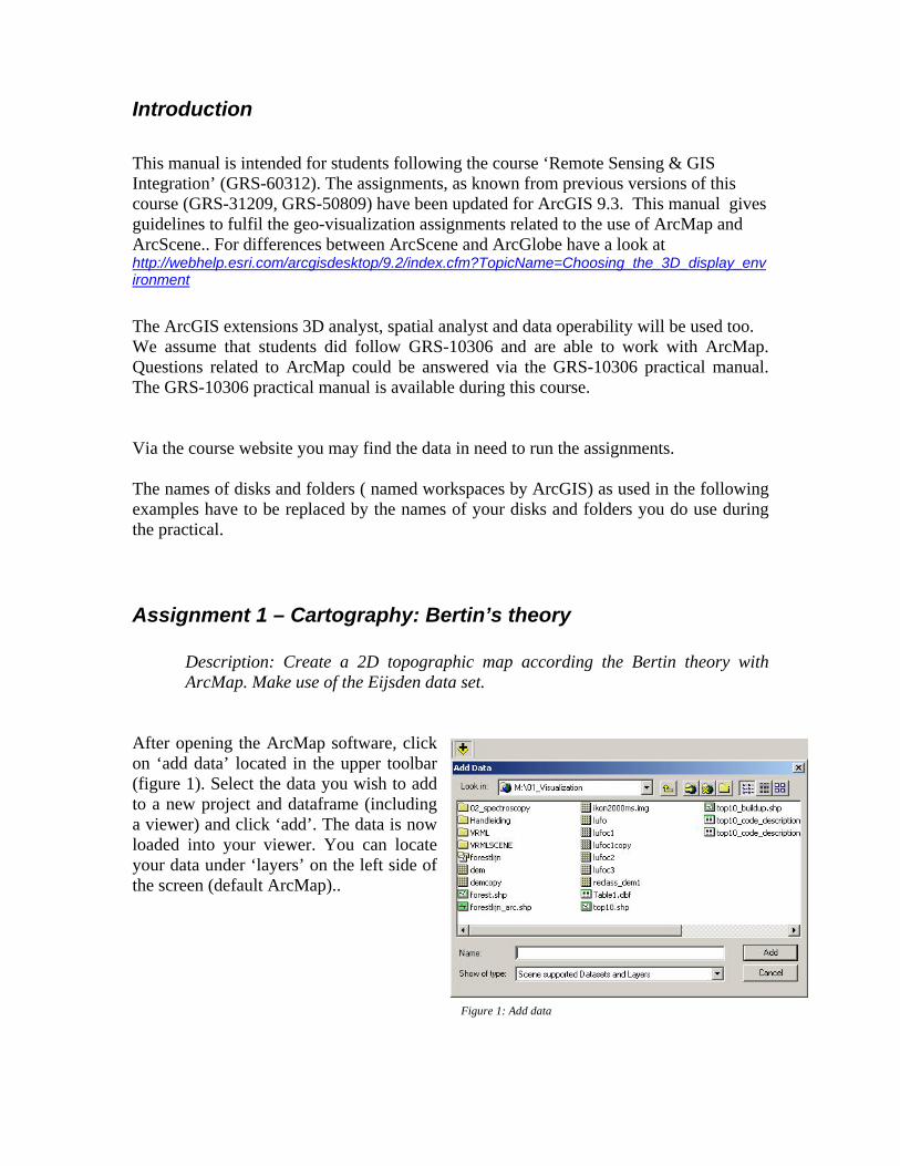
After opening the ArcMap software, click on ‘add data’ located in the upper toolbar (figure 1). Select the data you wish to add to a new project and dataframe (including a viewer) and click ‘add’. The data is now loaded into your viewer. You can locate your data under ‘layers’ on the left side of the screen (default ArcMap)..

Figure 1: Add data

WUR-CGI-2008/2009 4

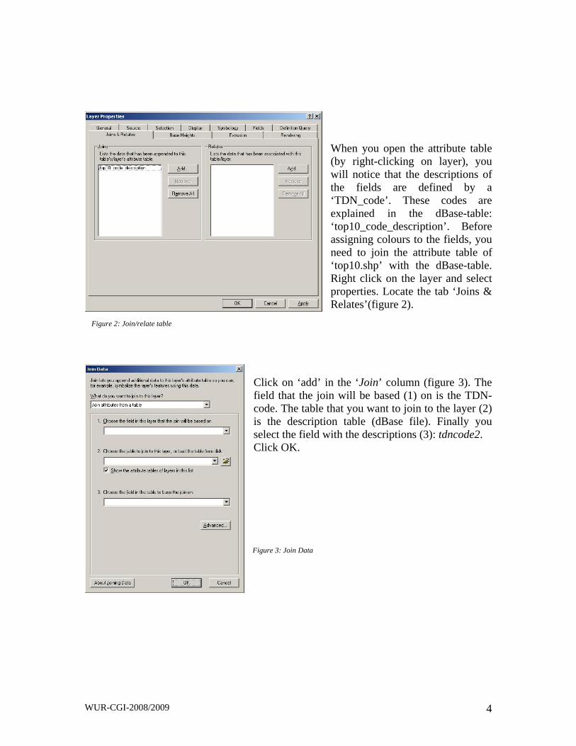
Figure 3: Join Data

When you open the attribute table (by right-clicking on layer), you will notice that the descriptions of the fields are defined by a ‘TDN_code’. These codes are explained in the dBase-table: ‘top10_code_description’. Before assigning colours to the fields, you need to join the attribute table of ‘top10.shp’ with the dBase-table. Right click on the layer and select properties. Locate the tab ‘Joins & Relates’(figure 2).

Click on ‘add’ in the ‘Join’ column (figure 3). The field that the join will be based (1) on is the TDN-code. The table that you want to join to the layer (2) is the description table (dBase file). Finally you select the field with the descriptions (3): tdncode2. Click OK.

Figure 2: Join/relate table

WUR-CGI-2008/2009 5

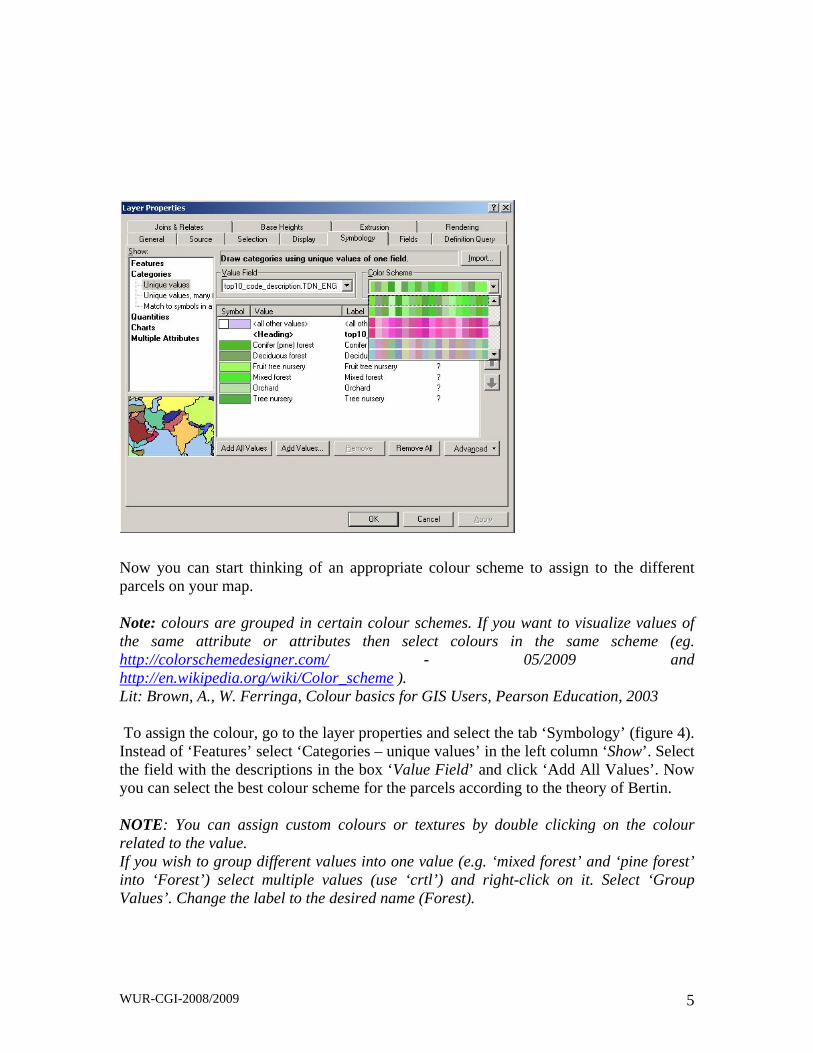
Now you can start thinking of an appropriate colour scheme to assign to the different parcels on your map. Note: colours are grouped in certain colour schemes. If you want to visualize values of the same attribute or attributes then select colours in the same scheme (eg. http://colorschemedesigner.com/ - 05/2009 and http://en.wikipedia.org/wiki/Color_scheme ). Lit: Brown, A., W. Ferringa, Colour basics for GIS Users, Pearson Education, 2003 To assign the colour, go to the layer properties and select the tab ‘Symbology’ (figure 4). Instead of ‘Features’ select ‘Categories – unique values’ in the left column ‘Show’. Select the field with the descriptions in the box ‘Value Field’ and click ‘Add All Values’. Now you can select the best colour scheme for the parcels according to the theory of Bertin. NOTE: You can assign custom colours or textures by double clicking on the colour related to the value. If you wish to group different values into one value (e.g. ‘mixed forest’ and ‘pine forest’ into ‘Forest’) select multiple values (use ‘crtl’) and right-click on it. Select ‘Group Values’. Change the label to the desired name (Forest).

WUR-CGI-2008/2009 6

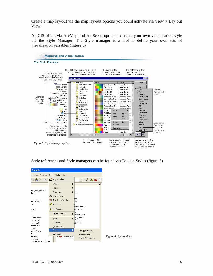
Create a map lay-out via the map lay-out options you could activate via View > Lay out View. ArcGIS offers via ArcMap and ArcScene options to create your own visualisation style via the Style Manager. The Style manager is a tool to define your own sets of visualization variables (figure 5)

Style references and Style managers can be found via Tools > Styles (figure 6)

Figure 5: Style Manager options

Figure 6: Style options

WUR-CGI-2008/2009 7

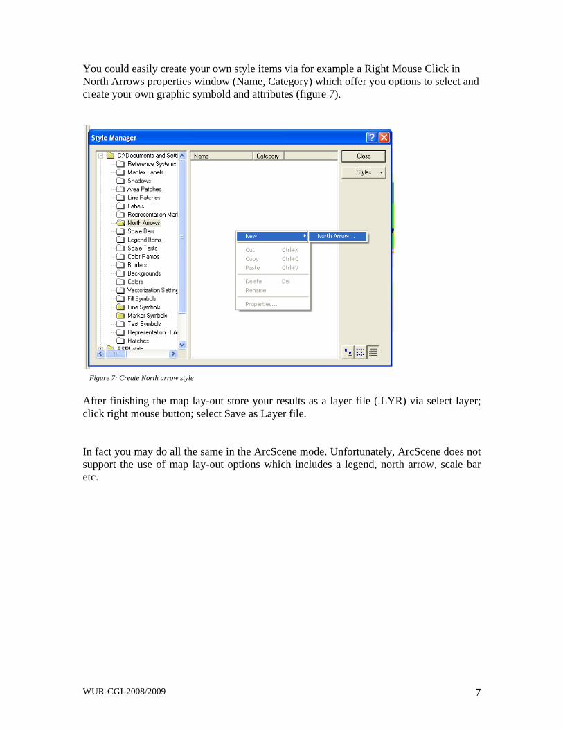
You could easily create your own style items via for example a Right Mouse Click in North Arrows properties window (Name, Category) which offer you options to select and create your own graphic symbold and attributes (figure 7).

After finishing the map lay-out store your results as a layer file (.LYR) via select layer; click right mouse button; select Save as Layer file. In fact you may do all the same in the ArcScene mode. Unfortunately, ArcScene does not support the use of map lay-out options which includes a legend, north arrow, scale bar etc.

Figure 7: Create North arrow style

WUR-CGI-2008/2009 8

Assignment 2 – The 3rd dimension: using DEM

Description: Create a 2.5 D topographic map according the Bertin theory with ARC Scene by draping on a DEM. Make use of the Eijsden data set.

Add the layer file or topographic shapefile and your DEM raster file to ArcScene. Next,

to drape your shapefile onto the DEM, right click your topographic shapefile and select properties. Move to the tab ‘Base Heights’ (figure 8). Click the radio button ‘Obtain heights for layer from surface’ and select your DEM. Click ‘OK’. Play around with the options custom to exaggerate the vertical dimension, and offset

You can remove your DEM layer from the view by making it invisible in the Scene layer window. NOTE: ARC Scene may reply with an error when trying to import a raster file, such as your DEM. To solve this problem, go to the ARC toolbox, located under the red toolbox icon (figure 9) and select the ‘Reclassify’ tool. This tool is located under ‘Spatial Analyst Tools’ > ‘Reclass’. Input a raster file in the ‘Input raster’ field and press ‘OK’. You need to do this only for one raster file. After this procedure, ARC Scene is again able to handle any raster file.

Figure 8: Base Heights (poly)

Figure 9: Toolbox

WUR-CGI-2008/2009 9

Assignment 3 – Aerial Photo Drape

Description: Create a 2,5 D map by draping aerial pictures on the DEM Make use of the Eijsden data set.

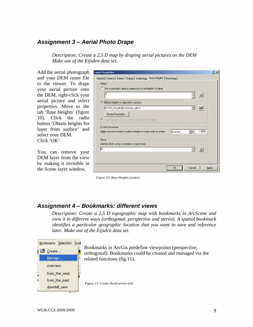
Add the aerial photograph and your DEM raster file to the viewer. To drape your aerial picture onto the DEM, right-click your aerial picture and select properties. Move to the tab ‘Base Heights’ (figure 10). Click the radio button ‘Obtain heights for layer from surface’ and select your DEM. Click ‘OK’. You can remove your DEM layer from the view by making it invisible in the Scene layer window.

Assignment 4 – Bookmarks: different views Description: Create a 2,5 D topographic map with bookmarks in ArcScene and view it in different ways (orthogonal, perspective and stereo). A spatial bookmark identifies a particular geographic location that you want to save and reference later. Make use of the Eijsden data set.

Bookmarks in ArcGis predefine viewpoints (perspective, orthogonal). Bookmarks could be created and managed via the related functions (fig.11).

Figure 10: Base Heights (raster)

Figure 11: Create North arrow style

WUR-CGI-2008/2009 10

NOTE: Bookmarks may be used in any view window. Make use of the Add Viewer and Viewer Manager functions to subsequently create and manage extra view windows (figure 12)

Via View >View settings (figure 13) you could easily change between viewers and view settings. By activating the Stereo radio button you may have a ‘real’ 3D view if you make use of a stereo glasses (in this case the one with a red and a blue glass) to stimulate stereopsis (see: http://en.wikipedia.org/wiki/Stereopsis ).

Figure 13: View settings

Figure 12: Add and Manage Viewers

WUR-CGI-2008/2009 11

Assignment 5 – Extrusion: the 3rd dimension of features

Description: Create a 3 D topographic map according the Bertin theory with arcview by extruding build up areas and forests. Make use of the Eijsden data set.

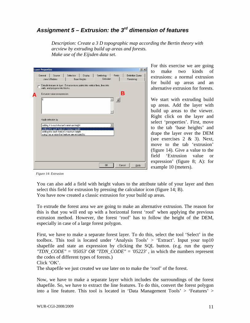
For this exercise we are going to make two kinds of extrusions: a normal extrusion for build up areas and an alternative extrusion for forests. We start with extruding build up areas. Add the layer with build up areas to the viewer. Right click on the layer and select ‘properties’. First, move to the tab ‘base heights’ and drape the layer over the DEM (see exercises 2 & 3). Next, move to the tab ‘extrusion’ (figure 14). Give a value to the field ‘Extrusion value or expression’ (figure 8; A): for example 10 (meters).

You can also add a field with height values to the attribute table of your layer and then select this field for extrusion by pressing the calculator icon (figure 14; B). You have now created a classic extrusion for your build up areas. To extrude the forest area we are going to make an alternative extrusion. The reason for this is that you will end up with a horizontal forest ‘roof’ when applying the previous extrusion method. However, the forest ‘roof’ has to follow the height of the DEM, especially in case of a large forest polygon. First, we have to make a separate forest layer. To do this, select the tool ‘Select’ in the toolbox. This tool is located under ‘Analysis Tools’ > ‘Extract’. Input your top10 shapefile and state an expression by clicking the SQL button. (e.g. run the query "TDN_CODE" = '05053' OR "TDN_CODE" = '05223' , in which the numbers represent the codes of different types of forests.) Click ‘OK’. The shapefile we just created we use later on to make the ‘roof’ of the forest. Now, we have to make a separate layer which includes the surroundings of the forest shapefile. So, we have to extract the line features. To do this, convert the forest polygon into a line feature. This tool is located in ‘Data Management Tools’ > ‘Features’ >

Figure 14: Extrusion

A B

WUR-CGI-2008/2009 12

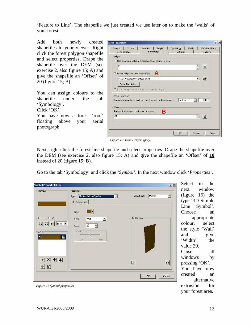
‘Feature to Line’. The shapefile we just created we use later on to make the ‘walls’ of your forest. Add both newly created shapefiles to your viewer. Right click the forest polygon shapefile and select properties. Drape the shapefile over the DEM (see exercise 2, also figure 15; A) and give the shapefile an ‘Offset’ of 20 (figure 15; B). You can assign colours to the shapefile under the tab ‘Symbology’. Click ‘OK’. You have now a forest ‘roof’ floating above your aerial photograph. Next, right click the forest line shapefile and select properties. Drape the shapefile over the DEM (see exercise 2, also figure 15; A) and give the shapefile an ‘Offset’ of 10 instead of 20 (figure 15; B). Go to the tab ‘Symbology’ and click the ‘Symbol’. In the next window click ‘Properties’.

Select in the next window (figure 16) the type ‘3D Simple Line Symbol’. Choose an

appropriate colour, select the style ‘Wall’ and give ‘Width’ the value 20. Close all windows by pressing ‘OK’. You have now created an

alternative extrusion for your forest area.

Figure 15: Base Heights (poly)

A

B

Figure 16 Symbol properties

WUR-CGI-2008/2009 13

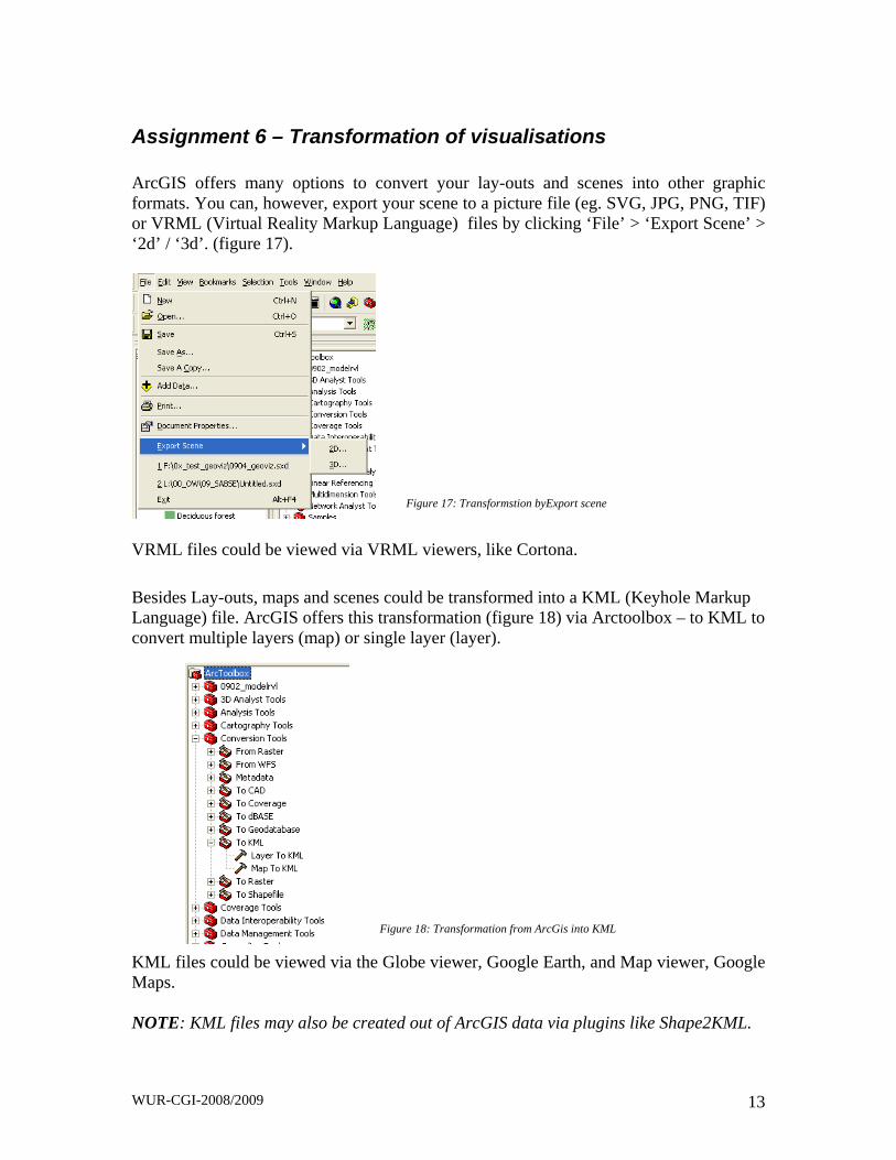
Assignment 6 – Transformation of visualisations ArcGIS offers many options to convert your lay-outs and scenes into other graphic formats. You can, however, export your scene to a picture file (eg. SVG, JPG, PNG, TIF) or VRML (Virtual Reality Markup Language) files by clicking ‘File’ > ‘Export Scene’ > ‘2d’ / ‘3d’. (figure 17).

VRML files could be viewed via VRML viewers, like Cortona. Besides Lay-outs, maps and scenes could be transformed into a KML (Keyhole Markup Language) file. ArcGIS offers this transformation (figure 18) via Arctoolbox – to KML to convert multiple layers (map) or single layer (layer).

KML files could be viewed via the Globe viewer, Google Earth, and Map viewer, Google Maps. NOTE: KML files may also be created out of ArcGIS data via plugins like Shape2KML.

Figure 17: Transformstion byExport scene

Figure 18: Transformation from ArcGis into KML

WUR-CGI-2008/2009 14

Figure 20: Texturized forest

Assignment 7 – Texture mapping for more realistic scenes

Description: Give the extruding forests and build up areas in Arc Scene a texture instead of only a colour. Make use of the Eijsden data set.

Right click the extruded shapefile that you want to give a texture. Go to the tab ‘Symbology’. Click ‘Symbol’ and next ‘Properties’. In the symbol property editor (figure 19) select as ‘Type’ a ‘3d texture line Symbol’ for the ‘walls’ of your forest, and a ‘3d texture fill symbol’ for the ‘roof’ of your forest and the build up areas.

You are now prompted to import an image file that will be used as a texture. Choose for example bark for the ‘walls’ of your forest and green vegetation for the ‘roof’ of the forest (figure 20). Give the ‘walls’ of the forest a vertical orientation and a width of 20 (note: you have to set the offset of your forest ‘walls’ back to 0). You have now created texturized 3d extrusions.

Figure 19: 3d texture

WUR-CGI-2008/2009 15

Assignment 8 – 3D Marker Symbol using 3D objects

Description: Create in Arc Scene a 2,5 D topographic map on a DEM with 3D marker symbols. Make use of the Eijsden data set.

Since 3D marker symbols can only be placed on point features, we have to create a new point shapefile. Go to ARC Catalog, browse to your workspace and click ‘File’ > ‘New’ > ‘Shapefile’. Next, fill in an appropriate name for your shapefile (e.g. ‘3dsymbols’), select the feature type ‘point’, and click ‘edit’ to change the spatial reference of your shapefile. Click ‘Import’ and select the dataset of which you want to import the coordinate system (e.g. the aerial photograph). Click two times ‘OK’ to create your new point shapefile.

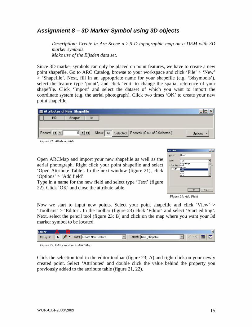
Open ARCMap and import your new shapefile as well as the aerial photograph. Right click your point shapefile and select ‘Open Attribute Table’. In the next window (figure 21), click ‘Options’ > ‘Add field’. Type in a name for the new field and select type ‘Text’ (figure 22). Click ‘OK’ and close the attribute table. Now we start to input new points. Select your point shapefile and click ‘View’ > ‘Toolbars’ > ‘Editor’. In the toolbar (figure 23) click ‘Editor’ and select ‘Start editing’. Next, select the pencil tool (figure 23; B) and click on the map where you want your 3d marker symbol to be located.

Click the selection tool in the editor toolbar (figure 23; A) and right click on your newly created point. Select ‘Attributes’ and double click the value behind the property you previously added to the attribute table (figure 21, 22).

Figure 21: Attribute table

Figure 21: Add Field

Figure 23: Editor toolbar in ARC Map

A B

WUR-CGI-2008/2009 16

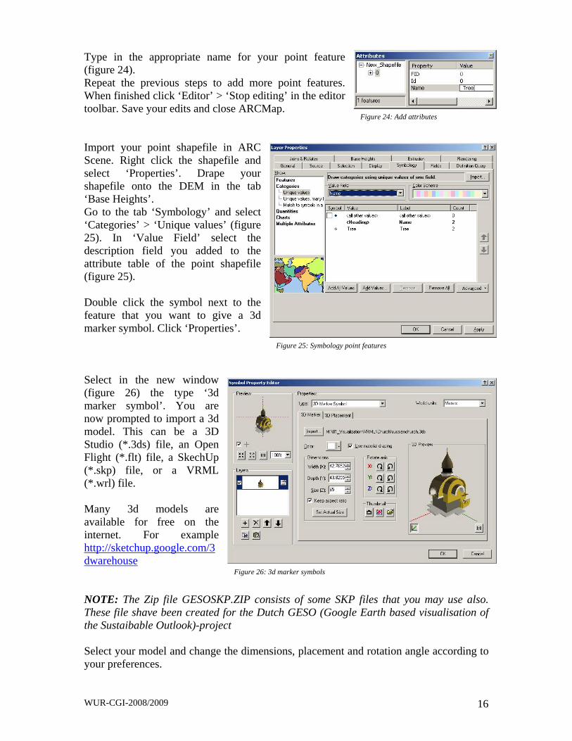
Type in the appropriate name for your point feature (figure 24). Repeat the previous steps to add more point features. When finished click ‘Editor’ > ‘Stop editing’ in the editor toolbar. Save your edits and close ARCMap. Import your point shapefile in ARC Scene. Right click the shapefile and select ‘Properties’. Drape your shapefile onto the DEM in the tab ‘Base Heights’. Go to the tab ‘Symbology’ and select ‘Categories’ > ‘Unique values’ (figure 25). In ‘Value Field’ select the description field you added to the attribute table of the point shapefile (figure 25). Double click the symbol next to the feature that you want to give a 3d marker symbol. Click ‘Properties’. Select in the new window (figure 26) the type ‘3d marker symbol’. You are now prompted to import a 3d model. This can be a 3D Studio (*.3ds) file, an Open Flight (*.flt) file, a SkechUp (*.skp) file, or a VRML (*.wrl) file. Many 3d models are available for free on the internet. For example http://sketchup.google.com/3dwarehouse NOTE: The Zip file GESOSKP.ZIP consists of some SKP files that you may use also. These file shave been created for the Dutch GESO (Google Earth based visualisation of the Sustaibable Outlook)-project Select your model and change the dimensions, placement and rotation angle according to your preferences.

Figure 24: Add attributes

Figure 25: Symbology point features

Figure 26: 3d marker symbols

WUR-CGI-2008/2009 17

Return to the layer properties window (figure 25) and repeat previous steps for the other point features. When finished click ‘OK’. You have now created a point layer with 3d marker symbols. NOTE: The creation of a point feature layer to be able to use 3D marker symbols is also possible by using the ArcToolbox > data management tools > Features by which you could adapt the feature type of available layers.

Assignment 9 – Animation to show changes

Description: Create animations in ArcScene, which shows the 2.5 D topographic map on a DEM. Make use of the Eijsden data set.

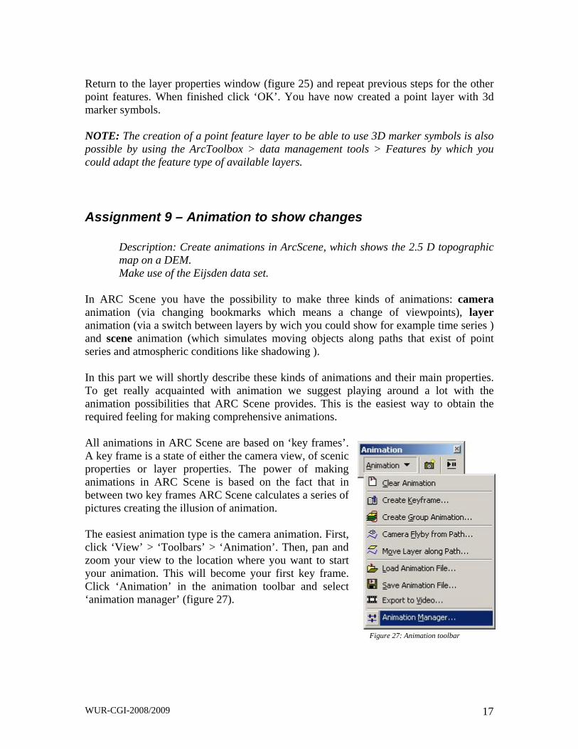
In ARC Scene you have the possibility to make three kinds of animations: camera animation (via changing bookmarks which means a change of viewpoints), layer animation (via a switch between layers by wich you could show for example time series ) and scene animation (which simulates moving objects along paths that exist of point series and atmospheric conditions like shadowing ). In this part we will shortly describe these kinds of animations and their main properties. To get really acquainted with animation we suggest playing around a lot with the animation possibilities that ARC Scene provides. This is the easiest way to obtain the required feeling for making comprehensive animations. All animations in ARC Scene are based on ‘key frames’. A key frame is a state of either the camera view, of scenic properties or layer properties. The power of making animations in ARC Scene is based on the fact that in between two key frames ARC Scene calculates a series of pictures creating the illusion of animation. The easiest animation type is the camera animation. First, click ‘View’ > ‘Toolbars’ > ‘Animation’. Then, pan and zoom your view to the location where you want to start your animation. This will become your first key frame. Click ‘Animation’ in the animation toolbar and select ‘animation manager’ (figure 27).

Figure 27: Animation toolbar

WUR-CGI-2008/2009 18

Select ‘Camera’ in the field ‘Key frame of type’ (figure 28). Click ‘Create’. In the next window (figure 29), choose type ‘camera’, make a new ‘destination track’ and give your key frame an appropriate name. Click ‘Create’.

Change the camera view to the next scene and repeat the previous steps for every key frame to create your flight path. To play your animation press the animation control button on the animation toolbar (figure 27). Another way to make a flight path is by drawing a line with the 3d graphic toolbar (figure 30). This toolbar is located under ‘View’ > ‘Toolbars’ > ‘3d Graphics’. Draw your flight path. Then, select ‘Camera Flyby from Path’ in the animation toolbar (figure 27) and fill in the specified parameters. Play with these parameters to see how they affect your animation.

Figure 28: Animation manager

Figure 29: Create key frame

Figure 30: 3d graphic toolbars

WUR-CGI-2008/2009 19

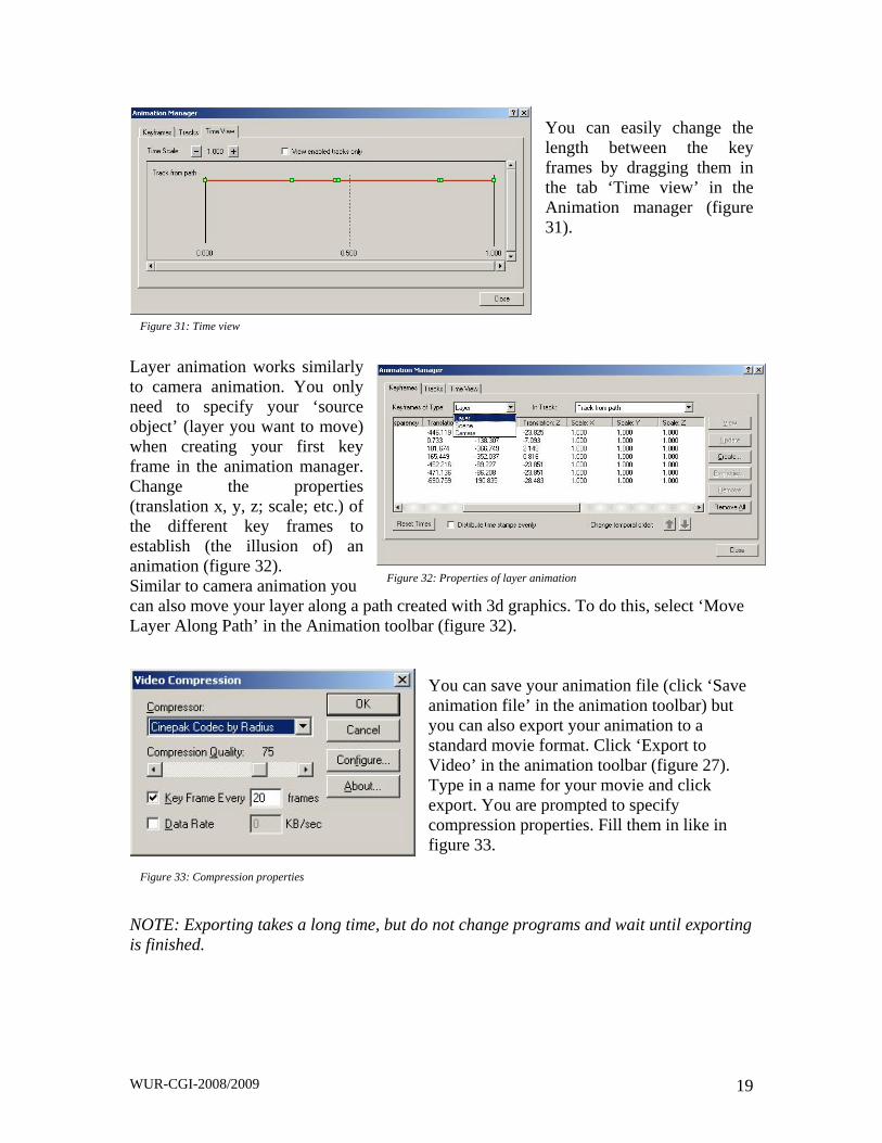
You can easily change the length between the key frames by dragging them in the tab ‘Time view’ in the Animation manager (figure 31).

Layer animation works similarly to camera animation. You only need to specify your ‘source object’ (layer you want to move) when creating your first key frame in the animation manager. Change the properties (translation x, y, z; scale; etc.) of the different key frames to establish (the illusion of) an animation (figure 32). Similar to camera animation you can also move your layer along a path created with 3d graphics. To do this, select ‘Move Layer Along Path’ in the Animation toolbar (figure 32).

You can save your animation file (click ‘Save animation file’ in the animation toolbar) but you can also export your animation to a standard movie format. Click ‘Export to Video’ in the animation toolbar (figure 27). Type in a name for your movie and click export. You are prompted to specify compression properties. Fill them in like in figure 33.

NOTE: Exporting takes a long time, but do not change programs and wait until exporting is finished.

Figure 31: Time view

Figure 32: Properties of layer animation

Figure 33: Compression properties