manufacturing and characterization of sustainable and
TRANSCRIPT
Manufacturing and Characterization of Sustainable and
Multifunctional Composite Structures
Miguel Diogo Milheiro Lonet de Carvalho e Branco
Thesis to obtain the Master of Science Degree in
Mechanical Engineering
Supervisors: Prof. Virgínia Isabel Monteiro Nabais Infante
Prof. Maria de Fátima Reis Vaz
Examination Committee
Chairperson: Prof. Luís Filipe Galrão dos Reis
Supervisor: Prof. Virgínia Isabel Monteiro Nabais Infante
Member of the Committee: Prof. Rosa Maria Marquito Marat-Mendes
November 2018

ii

iii
―If you want to find the secrets of the universe, think in terms of energy, frequency and vibration.‖
Nikola Tesla

iv
Acknowledgements
To my family for the unconditional support and love.
A special thanks to my supervisor Professor Virgínia Infante and co-supervisor Professor Maria de
Fátima Vaz, for the availability and guidance throughout the project.
Eng. Luís Amorim for the shared experience and knowledge.
Rafael and Bruno from PIEP’s composites laboratory, for their support in the vacuum infusion process.
Eng. Andreia Vilela, from PIEP, for her collaboration in the mechanical tests performed.
Professors Luís Reis, Manuel Freitas and Rosa Marat-Mendes for their assistance with the C-Scan.
Professor António Ramos Silva for the availability to perform the thermography analysis.

v
Abstract
This work consisted on the production, mechanical characterization and damage assessment of
carbon fiber laminates, produced by resin vacuum infusion, with three different stacking sequences –
an aeronautical standard, provided by Embraer, and two bio-inspired.
The mechanical characterization was accomplished by applying uniaxial tensile, interlaminar shear
strength and drop weight impact tests.
The damage, induced in the impacted specimens, was assessed by three non-destructive techniques
– visual inspection, ultrasonic testing (C-Scan) and thermography.
Tensile test results were in accordance with the literature. The interlaminar shear strength test
revealed more reliable results for the bio-inspired laminates, in accordance with the literature. In the
impact test results, it is suggested an energy transition (around 25 J) above which bio-inspired
laminates begin to absorb more energy than the aeronautical standard.
Regarding damage assessment, the visual inspection identified different types of damage. The
ultrasonic inspection revealed the damaged areas, although the signal dispersion and the reduced
number of samples per test condition. Finally, thermography analysis was applied to a set of
specimens without impact and specimens impacted with 13.5 J. It was detected what suggests to be
delamination, for an impacted specimen. This result seems to validate the increasing application of
thermography in high performance industries, as the aeronautical.
Keywords: CFRP; Bio-inspired composites; Vacuum Infusion; Low Velocity Impact.
vi
Resumo
O presente trabalho consistiu na produção, caracterização mecânica e avaliação do dano de
laminados de fibra de carbono, produzidos pelo processo de infusão de resina por vácuo, com três
sequências de empilhamento distintas – uma de controlo da indústria aeronáutica, fornecida pela
Embraer, e duas bio-inspiradas.
A caracterização mecânica dos laminados foi realizada através de ensaios de tracção uniaxial,
resistência interlaminar e impacto por queda de peso.
Para a avaliação do dano foram aplicados três ensaios não-destrutivos – inspecção visual, varrimento
por ultrasons (C-Scan) e termografia.
O ensaio de tracção produziu os resultados esperados. No ensaio da resistência interlaminar os
laminados bio-inspirados sugerem, de acordo com a literatura, os resultados mais fiáveis. No ensaio
de impacto é sugerida uma energia de transição (cerca de 25 J) para a qual os laminados bio-
inspirados passam a absorver mais energia que o laminado de controlo.
Nos ensaios não-destrutivos, a inspecção visual identificou diferentes tipos de dano visível. O
varrimento por ultrasons revelou as áreas danificadas pelo impacto, apesar da dispersão do sinal e do
reduzido número de provetes por condição de teste. Por fim, na termografia, aplicada apenas a
alguns provetes após produção (sem impacto) e provetes impactados com 13,5 J, foi detectada o que
sugere ser a forma típica da delaminação, num provete impactado - o que parece validar a aplicação
crescente da termografia em indústrias de elevado desempenho, como a aeronáutica.
Plavras-chave: CFRP; Compósitos bio-inspirados; Infusão por vácuo; Impacto de baixa velocidade.
vii
Contents
Acknowledgements iv
Abstract v
Resumo vi
Contents vii
List of Tables ix
List of Figures x
Acronyms xii
Symbols xiii
1. Introduction 1
1.1 Motivation 1
1.2 Background 2
1.3 Objectives 3
1.4 Thesis Structure 3
2. State of the Art 4
2.1 Composite Materials Introduction 4
2.2 Composite Materials in the Aeronautical Industry 6
2.3 Production Processes 10
2.4 Mechanical Tests 12
2.4.1 Introduction to Failure Modes 14
2.5 Non-Destructive Techniques (NDT) 16
2.6 Bio-inspired Solutions 18
3. Experimental Work 22
3.1 Material System 22
3.1.1 Fiber 22
3.1.2 Resin 23
3.2 Stacking Sequences 24
3.3 Production of the laminates 24
3.3.1 Unpacking and cutting 24
3.3.2 Resin Infusion Procedure 25
3.3.3 Process modification techniques 27
4. Mechanical tests 28
4.1 Tensile Properties of Polymer Matrix Composite Materials 28
4.2 Interlaminar Shear Strength Test [ILSS] 32
4.3 Impact Test 34
5. Results and Discussion 37
5.1 Tensile Test 37

viii
5.1.1 LS stacking sequence 37
5.1.2 HL stacking sequence 38
5.1.3 HL-S stacking sequence 39
5.1.4 Discussion 40
5.2 Interlaminar Shear Strength Test [ILSS] 43
5.2.1 LS stacking sequence 43
5.2.2 HL stacking sequence 44
5.2.3 HL-S stacking sequence 45
5.2.4 Discussion 45
5.3 Impact Test 50
5.3.1 Impact with 13.5 [J] 53
5.3.2 Impact with 25 [J] 54
5.3.3 Impact with 40 [J] 56
5.3.4 Impact with 80 [J] 58
5.3.5 Discussion 59
6. Non-destructive testing 61
6.1 Visual Inspection 61
6.2 C-Scan 62
6.3 Thermography 66
7. Conclusions 69
8. Future Work 70
9. References 71
Annex 76
A. Mechanical Tests for Composite Materials 76
B. Stacking sequence configuration 79
C. Tensile Test 79
C.1 Tensile Test – Specimens dimensions 79
C.2 Tensile Test – Failure Modes Observation 80
D. Interlaminar Shear Strength Test 83
E. Impact Test 84
F. C-Scan 89
ix
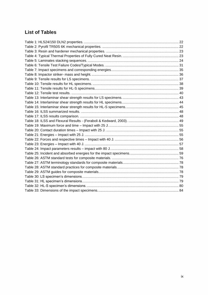
List of Tables
Table 1: HLS24/150 DLN2 properties. .................................................................................................. 22 Table 2: Pyrofil TR50S 6K mechanical properties. ............................................................................... 22 Table 3: Resin and hardener mechanical properties. ........................................................................... 23 Table 4: Typical Thermal Properties of Fully Cured Neat Resin. .......................................................... 23 Table 5: Laminates stacking sequences. .............................................................................................. 24 Table 6: Tensile Test Failure Codes/Typical Modes. ............................................................................ 31 Table 7: Impact specimens and corresponding energies. ..................................................................... 35 Table 8: Impactor striker- mass and height. .......................................................................................... 36 Table 9: Tensile results for LS specimens. ........................................................................................... 37 Table 10: Tensile results for HL specimens. ......................................................................................... 38 Table 11: Tensile results for HL-S specimens....................................................................................... 39 Table 12: Tensile test results. ............................................................................................................... 40 Table 13: Interlaminar shear strength results for LS specimens. .......................................................... 43 Table 14: Interlaminar shear strength results for HL specimens........................................................... 44 Table 15: Interlaminar shear strength results for HL-S specimens. ...................................................... 45 Table 16: ILSS summarized results. ..................................................................................................... 48 Table 17: ILSS results comparison. ...................................................................................................... 48 Table 18: ILSS and Flexural Results - (Feraboli & Kedward, 2003). .................................................... 49 Table 19: Maximum force and time – Impact with 25 J. ........................................................................ 55 Table 20: Contact duration times – Impact with 25 J. ........................................................................... 55 Table 21: Energies – Impact with 25 J. ................................................................................................. 55 Table 22: Forces and respective times – Impact with 40 J. .................................................................. 56 Table 23: Energies – Impact with 40 J. ................................................................................................. 57 Table 24: Impact parameters results – impact with 80 J. ...................................................................... 58 Table 25: Incident and absorbed energies for the impact specimens. .................................................. 59 Table 26: ASTM standard tests for composite materials. ..................................................................... 76 Table 27: ASTM terminology standards for composite materials. ......................................................... 78 Table 28: ASTM standard practices for composite materials. ............................................................... 78 Table 29: ASTM guides for composite materials................................................................................... 78 Table 30: LS specimen’s dimensions. ................................................................................................... 79 Table 31: HL specimen’s dimensions. ................................................................................................... 79 Table 32: HL-S specimen’s dimensions. ............................................................................................... 80 Table 33: Dimensions of the impact specimens. ................................................................................... 84

x
List of Figures
Figure 1: a) Ancient composites: plywood used in Egypt; b) Egyptian Ptolemaic gilt cartonnage
sarcophagus mask and c) mud and straw bricks. ................................................................................... 4
Figure 2: Composite material generic composition. ................................................................................ 4 Figure 3: Types of matrices. .................................................................................................................... 5 Figure 4: Types of reinforcements. .......................................................................................................... 5 Figure 5: a) The Wright brother’s model; b) De Havilland Mosquito fuselage. ....................................... 6 Figure 6: Materials distribution for the Boeing 787. ................................................................................. 7 Figure 7: Airbus composite structural weight development. .................................................................... 7 Figure 8: Airbus A380 design criteria (Pora, 2001). ................................................................................ 8 Figure 9: 787 Dry fiber/infused parts include (left to right) ailerons and flaps, fuselage frames and the
aft pressure bulkhead (APB) of the fuselage (Dry Composites, 2013). .................................................. 9 Figure 10: A380 Aft Pressure Bulkhead and A400 pressurized Cargo Door (Dry Composites, 2013). .. 9 Figure 11: The Bombardier C Series wing (left) and Irkut MS21 wing (right) both are made from dry
fiber preforms and resin infusion (Dry Composites, 2013). ..................................................................... 9 Figure 12: a) Aircraft maintenance; b) debris impact; c) bird-strike. ..................................................... 12 Figure 13: a) Space Shuttle Columbia; b) foam from simulation; c) CFRP panel in NASA’s test bench.
............................................................................................................................................................... 13 Figure 14: Possible failure modes in composites – as illustrated in (Safri et al.,2014). ........................ 14 Figure 15: Comparison between Quasi-Static Indentation and Low Velocity Impact (Lawrence &
Emerson, 2012). .................................................................................................................................... 15 Figure 16: Relationship between Interlaminar shear strength and Void Content for unidirectional HTS
carbon fibers in an ERLA 4617 epoxy-resin matrix (source: Stone D. and Clarke B. (1974). Non-
destructive Determination of the Void Content in Carbon Fiber Reinforced Plastics by Measurement of
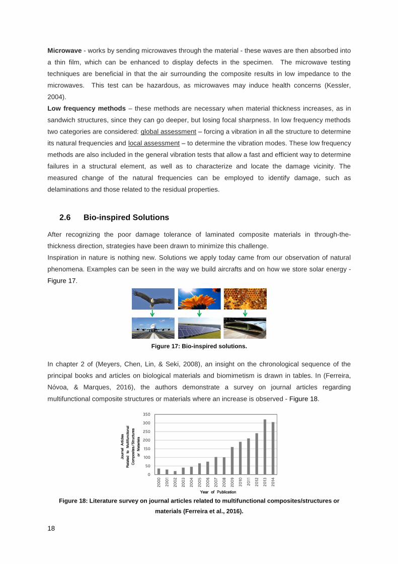
Ultrasonic Attenuation, RAE Technical Report 74162) – as cited in (Smith, 2009). ............................. 17 Figure 17: Bio-inspired solutions. .......................................................................................................... 18 Figure 18: Literature survey on journal articles related to multifunctional composites/structures or
materials (Ferreira et al., 2016). ............................................................................................................ 18 Figure 19: Hierarchy of crab exoskeleton – adapted from (Meyers et al., 2008). ................................. 19 Figure 20: a) Odontodactylus scyllarus - also known as mantis shrimp; b) Peacock mantis shrimp
striking a shell. ....................................................................................................................................... 20 Figure 21: Force generated by the Mantis shrimp strikes during impact (Patek & Caldwell, 2005). .... 21 Figure 22: Fabric DLN2 from Dynanotex (Angeloni - Fabrics Catalogue). ........................................... 22 Figure 23: a) Carbon fiber; b) laser cutting machine. ............................................................................ 24 Figure 24: a) Glass plate and blade on top of nylon blocks; b) release agent; c) sealant applied........ 25 Figure 25: a) Gum tape; b) fibers layup before infusion; c) peel-ply. .................................................... 25 Figure 26: a) Flow mesh; b) infusion spiral and PVC tube; c) identification of the oversized bag area.25 Figure 27: a) Vacuum pump; b) pressure indicator; c) resin weight measurement. ............................. 26 Figure 28: a) Air degassing unit; b) resin pot. ....................................................................................... 26 Figure 29: a) Resin progression during the infusion; b) post cure oven. .............................................. 26 Figure 30: Set-up with different parameters. ......................................................................................... 27 Figure 31: a) MTS model 45; b) specimen dimensions. ........................................................................ 29 Figure 32: Tensile specimens before testing......................................................................................... 30 Figure 33: Loading diagram of the ILSS test - (ISO 14130, 1997). ....................................................... 32 Figure 34: a) Shimatzu AG located at PIEP; b) ILSS specimen inserted in the testing machine. ........ 33 Figure 35: Example of specimen being examined in the magnifying glass. ......................................... 34 Figure 36: ASTM D2344 failure modes. ................................................................................................ 34 Figure 37: Fractovis Plus from CEAST and the representation of the strain gauge striker. ................. 34 Figure 38: a), b) Impact support fixture – ASTM illustration (a) and picture (b); c) Impact specimens. 35

xi
Figure 39: Tensile test - Load versus Displacement curve for LS specimens. ..................................... 37 Figure 40: Tensile test - Load versus Displacement curve for HL specimens. ..................................... 38 Figure 41: Tensile test - Load versus Displacement curve for HL-S specimens. ................................. 39 Figure 42: Young’s modulus vs. ply orientation for typical CFRP – adapted from (Moura et al., 2005).
............................................................................................................................................................... 41 Figure 43: Peak load average and respective intervals for the three stacking sequences. .................. 41 Figure 44: Failure mechanisms for fiber stress vs. fibers orientation (Souza, 2003). ........................... 42 Figure 45: Example of the LS2 specimen failure mode. ....................................................................... 42 Figure 46: Load versus displacement curves for LS specimens. .......................................................... 43 Figure 47: Load versus displacement curves for HL specimens. .......................................................... 44 Figure 48: Load versus displacement curves for HL-S specimens. ...................................................... 45 Figure 49: Pure shear stress state. ....................................................................................................... 46 Figure 50: Illustration of bending stresses location. .............................................................................. 46 Figure 51: Used geometry versus recommended geometry by ASTM D2344. .................................... 47 Figure 52: Illustration of the typical crack initiation and delamination. .................................................. 47 Figure 53: Flexure behavior for the LS 4 specimen. ............................................................................. 48 Figure 54: Interlaminar shear strength comparison. ............................................................................. 48 Figure 55: Types of response relating contact (impact) duration (Olsson, Donadon, & Falzon, 2006). 51 Figure 56: Impact test curves - 13.5 J. .................................................................................................. 53 Figure 57: Force vs. Displacement – Impact with 13.5 J. ..................................................................... 54 Figure 58: Impact test curves - 25 J. ..................................................................................................... 54 Figure 59: Force vs. Displacement - Impact with 25 J. ......................................................................... 55 Figure 60: Impact test curves - 40 J. ..................................................................................................... 56 Figure 61: Force vs. Displacement - Impact with 40 J. ......................................................................... 57 Figure 62: Impact test curves – 80 J. .................................................................................................... 58 Figure 63: Force vs. Displacement - Impact with 80 J. ......................................................................... 59 Figure 64: Externally visible damage types (ASTM D7136, 2015)........................................................ 61 Figure 65: Visual inspection for HL-1 specimen impacted with 80 J. .................................................... 62 Figure 66: Single element transducer – adapted from (Olympus). ....................................................... 63 Figure 67: Typical transducer beam (Olympus). ................................................................................... 63 Figure 68: Representation of the pressure gradients of beam (Olympus). ........................................... 63 Figure 69: a) Laboratory with Ultrapac II system associated with Ultrawin software; b) schematic view
of the ultrasonic system (Hasiotis, Badogiannis, & Tsouvalis, 2011). ................................................... 64 Figure 70: C-Scan image of HL 2 – 25 J specimen. ............................................................................. 65 Figure 71: Thermography performed in a) the engine cowl; b) flaps (Ralf, 2010). ............................... 66 Figure 72: Active thermography principle. ............................................................................................. 67 Figure 73: Thermography setup in FEUP’s laboratory. ......................................................................... 68 Figure 74: Specimen impacted with 13.5 J inspected by thermography. .............................................. 68 Figure 75: Stacking sequences configuration. ...................................................................................... 79 Figure 76: LS tensile specimens. .......................................................................................................... 80 Figure 77: HL tensile specimens. .......................................................................................................... 81 Figure 78: HL-S tensile specimens. ...................................................................................................... 82 Figure 79: LS interlaminar shear strength specimens. .......................................................................... 83 Figure 80: HL interlaminar shear strength specimens. ......................................................................... 83 Figure 81: HL-S interlaminar shear strength specimens. ...................................................................... 84 Figure 82: Impacted specimens: 13.5 J. ............................................................................................... 85 Figure 83: Impacted specimens: 25 J. .................................................................................................. 86 Figure 84: Impacted specimens: 40 J. .................................................................................................. 87 Figure 85: Impacted specimens: 80 J. .................................................................................................. 88 Figure 86: Parameterization 1 C-Scan figures. ..................................................................................... 89 Figure 87: Parameterization 2 C-Scan figures. ..................................................................................... 89 Figure 88: Parameterization 3 C-Scan figures. ..................................................................................... 89

xii
Acronyms
ACMA – American Composites Manufacturers Association
ASTM – American Society for Testing Materials
BVID – Barely Visible Impact Damage
CAI – Compression After Impact
CFRP – Carbon Fiber Reinforced Polymer(s)/Plastic(s)
EASA – European Aviation Safety Agency
FAA – Federal Aviation Administration
FOD – Foreign Object Damage/Debris
IAMAT – Introduction of Advanced Materials Technologies into new product development for the
mobility industries
IDMEC – Instituto de Engenharia Mecânica
ILSS – Interlaminar Shear Strength
IST – Instituto Superior Técnico
LCCF – Low Cost Composite Fabrication
LVI – Low Velocity Impact
NDT – Non-Destructive Techniques
OoA – Out of Autoclave
PIEP – Pólo de Inovação em Engenharia de Polímeros
QSI – Quasi-Static Indentation
RTM – Resin Transfer Molding
UD – Unidirectional
VARI – Vacuum Assisted Resin Infusion

xiii
Symbols
– impactor’s displacement
– clip gauge’s displacement at ith data point
– difference between two strain data points
– difference in applied tensile stress between two strain data points
– tensile strain at ith data point
– tensile stress at ith data point
– ultimate tensile strength
– average cross-sectional area
b – specimen’s width
– Young’s modulus
– absorbed energy
– kinetic energy
– incident energy (impact test)
– maximum energy (impact test)
– potential energy
– force
F1 – threshold force (impact test)
Fmax – maximum force (impact test)
- apparent interlaminar shear strength
g – acceleration due to gravity
h – specimen’s thickness
H – height (kinetic energy equation - impact test)
– clip gauge’s length
m – impactor’s mass
– load at ith data point
– maximum load observed during interlaminar shear strength test
- maximum load before failure (tensile test)
– time
t1 – time at threshold force
t Fmax – time at maximum force
tT – contact duration (impact test)
– impactor’s velocity at the time of initial contact
– impactor’s velocity


1
1. Introduction
1.1 Motivation
The motivation for this work can be divided in three vectors: 1) the weight reduction and improved
mechanical properties, such as specific modulus and specific strength, offered by composite materials
when compared to other conventional structural materials; 2) the development of a production process
that decreases costs and energy consumption (when compared to autoclave) and 3) bio-inspired
solutions that can result in improved mechanical behavior.
1) Weight reduction: has always been a leading factor in aircraft’s development. More than twenty
years ago, a weight saving of one pound (0.454 kg) represented a fuel saving, on a full-service
commercial aircraft, of about 1586 [liters/year] (Kaw, 1997).
Boeing estimated that the high use of carbon fiber and other composites offers weight savings, on
average, of about 20%, when compared to conventional aluminum designs (Boeing, 2006).
2) Out of Autoclave (OoA) composites: may cut the production time by 40% and the costs by 50%,
when compared with autoclave process - as expected by Spirit Aerosystems, a composites
manufacturer. For its Out of Autoclave (OoA) process, Spirit uses a multi-zone heated tool that
enables complete control of the composite curing, through real-time monitoring and feedback.
Components produced in this way may be field repairable because they won’t need autoclaves to re-
cure (Spirit Aerosystems, 2017).
Side benefits include the use of cheaper soft tooling that might not withstand autoclave cycles and
reduced risks of vacuum bag leaks, since autoclave pressure is not used.
On the other hand, some companies have noted that new composite production techniques allow the
manufacturing of more complex components that can be harder to repair (Derber, 2017).
To compete with metal part production economically, Low-Cost Composite Fabrication (LCCF)
techniques such as filament winding, vacuum assisted resin infusion (VARI), resin transfer molding
(RTM), Seemann Composites Resin Infusion Molding Process (SCRIMP) and other liquid infusion
process have evolved as alternatives to the prepregs/autoclave method (Chia, Lee, Yeo, & Tan,
2001).
Of course Out of Autoclave composites have disadvantages, being one the most pronounced the void
content. This process usually presents a 3-5% of voids, while the autoclave composites are produced
with less than 1%. An increase of 1-3% of voids can decrease mechanical properties by 20% (Boey &
Lye, 1992). Autoclave process applied in the production of aeronautical composites requires a
pressure chamber that, with the injection of liquid nitrogen, cures with 120-135 or 180°C, at pressures
up to 8 bar, occasionally with a post cure at higher temperatures (Soutis, 2005).
As rising fuel costs and concerns over the environmental effects became critical, airframe
manufacturers are pushed to improve aircraft efficiency. Out-of-Autoclave specific prepregs and resin
infused fabrics have been cured in microwave and conventional ovens (Witik, Gaille, Teuscher,
Ringwald, & Michaud, 2012). Resin infusion has been proved to reduce costs, as reinforcement
fabrics and resin are less expensive. Reductions in energy total cost were not significant. The Out-of-
2
Autoclave prepregs did not perform as well due to their higher costs, longer cycle times and the need
for lengthy de-bulking operations. Microwave curing also did not present significant improvements in
terms of cost reduction and environmental concerns, due to investment costs similarly to autoclave
and higher energy consumptions than traditional oven cure.
3) Bio-inspired solutions: anyone has ever touched a crustacean has observed its strong shell. These
shells, made of calcite or cuticle, are composed of structures that allow toughness up to three orders
of magnitude higher than the unstructured material alone. One of the most known crustaceans is the
shrimp. What many people don’t know is the 300 million year of marine evolution and adaptation this
species represents (Ribbans, 2015).
The mantis shrimp is not a simple shrimp, truth be told, is not even a shrimp, is a stomatopod. It is
called shrimp due to the similar appearance. The mantis in the name comes also from his similarity,
but this time to a praying mantis, furthermore, both share the same hunting strategies.
The most impressive aspect about the mantis shrimp is how it breaks shells with its clubs. The science
behind involves the hyperbolic paraboloid shape of its structure, located on top of the smasher, while
the stomatopod uses his muscles to compress it like a spring and holds it back with a latch
mechanism. It then releases this potential energy which allows driving the club forward at a much
higher velocity than would be possible relying on a single muscle.
But what is set to be applied in this work is what is seen at the micro and nano-scales – the helicoidal
layup. In the case of the mantis shrimp, the strands are bonded together in a mineralized matrix. The
material changes composition and strength through its structure. While the impact surface is incredibly
hard, the internal structure transitions smoothly to layers less hard, in order to allow the distribution of
a great impulse throughout the rest of the structure, allowing the mantis shrimp to punch several times
without breaking (Sandlin, 2014).
Despite the studies that have been developed regarding helicoidal structures, there is a lack of studies
about the interlaminar shear behavior, where failure is common in composite helicoidal laminates, and
assessing their mechanical performance under shear and normal stresses. Furthermore, the crack
mechanisms between the fiber layers of helicoidal structures are not well understood (Ribbans, 2015).
1.2 Background
The work presented was developed under the purview of a MIT Portugal’s project – IAMAT:
introduction of advanced materials technologies into new product development for the mobility
industries.
IAMAT’s project is composed by four faculties: University of Lisbon, University of Minho, University of
Porto and Massachusetts Institute of Technology; and two companies – Optimal Structures and the
aeronautical manufacturer Embraer. The project is divided in five working packages (WP):
WP1: Computational materials morphologies – material systems development based on advanced
computational and experimental techniques.
WP2: Sustainable multifunctional structures – manufacturing technologies for the production of the
new materials; multifunctional structures.
WP3: Management of uncertainty – analytical tools and implementation methods to evaluate the
economic and environmental impact of the new materials and manufacturing processes.

3
WP4: Supply chains towards sustainably – framework and tools for evaluating and quantifying the
supply chain impacts of product design choices.
WP5: Testbed – Embraer aerostructure.
Being part of the WP2, this work was developed at the University of Minho, with the collaboration of
the PhD student Luís Amorim. The carbon fiber laminates were produced at PIEP – an innovation
center for polymer engineering located at University of Minho campus, in Guimarães.
1.3 Objectives
The objectives of the work are:
1) Production of laminates with bio-inspired stacking sequences by an OoA process: vacuum bag
infusion;
2) Mechanical characterization of the laminates produced and comparison with a standard stacking
sequence;
3) Comparison of energy absorption between different stacking sequences;
4) Observation and discussion of the damage assessment with non-destructive techniques.
1.4 Thesis Structure
In chapter 2 the state of the art is presented, starting with a brief introduction of composite materials
and their application in the aeronautical industry. Then an overall view of the production processes for
composite materials is summarized. The following sub-chapter describes composites production
processes. In 2.4 mechanical tests are presented, with reference to annex A, where a list of composite
materials tests is presented, besides terminology, practices and guides. The selected mechanical
tests are indicated and an introduction on failure modes is developed. In 2.5, non-destructive
techniques for composite materials are also presented. The last sub-chapter of the state of the art is
2.6, where bio-inspired solutions are drawn, with focus to the mantis shrimp.
Chapter 3 develops the experimental work, with the material system properties in 3.1 (sub-chapters
3.1.1 for the fiber and 3.1.2 for the resin system). In 3.2 the stacking sequences applied for the
production of the laminates are presented (detailed in annex B) and in the sub-chapter 3.3, the
vacuum infusion process is explained with references to modification techniques in 3.3.3.
Chapter 4 explains the mechanical tests performed to characterize the laminates produced – with sub-
chapters 4.1 for the tensile test, 4.2 for interlaminar shear strength test and 4.3 for impact test.
Chapter 5 illustrates the results of the mechanical tests and draws its discussions. The sub-chapters
5.1 and 5.2 give the tensile and interlaminar shear strength results for each stacking sequence,
respectively. Sub-chapter 5.3 has the impact test results, divided in four impact energies – 13.5 J
(5.3.1), 25 J (5.3.2), 40 J (5.3.3) and 80 J (5.3.4).
Chapter 6 exhibits the three non-destructive techniques applied: visual inspection (6.1), ultrasonic test
C-Scan (6.2) and thermography (6.3). Chapter 7 compiles the conclusions of the work and chapter 8
indicates suggested future work. Chapter 9 lists the references invoked during the dissertation and the
annexes also contain information regarding: tensile testing (annex C), interlaminar shear strength test
(annex D), impact testing (annex E) and C-Scan imaging results (annex F).
4
2. State of the Art
2.1 Composite Materials Introduction
A composite material can be defined as the combination of two or more materials that do not dissolve
or merge completely in each other, with the purpose of obtaining improved mechanical properties for a
given application. The constituents remain separate and distinct within the composite material.
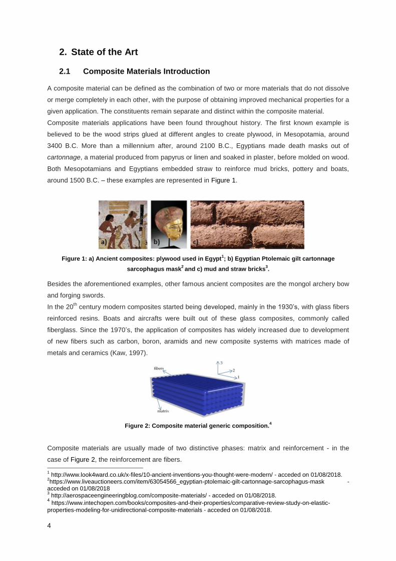
Composite materials applications have been found throughout history. The first known example is
believed to be the wood strips glued at different angles to create plywood, in Mesopotamia, around
3400 B.C. More than a millennium after, around 2100 B.C., Egyptians made death masks out of
cartonnage, a material produced from papyrus or linen and soaked in plaster, before molded on wood.
Both Mesopotamians and Egyptians embedded straw to reinforce mud bricks, pottery and boats,
around 1500 B.C. – these examples are represented in Figure 1.
Figure 1: a) Ancient composites: plywood used in Egypt1; b) Egyptian Ptolemaic gilt cartonnage
sarcophagus mask2
and c) mud and straw bricks3.
Besides the aforementioned examples, other famous ancient composites are the mongol archery bow
and forging swords.
In the 20th century modern composites started being developed, mainly in the 1930’s, with glass fibers
reinforced resins. Boats and aircrafts were built out of these glass composites, commonly called
fiberglass. Since the 1970’s, the application of composites has widely increased due to development
of new fibers such as carbon, boron, aramids and new composite systems with matrices made of
metals and ceramics (Kaw, 1997).
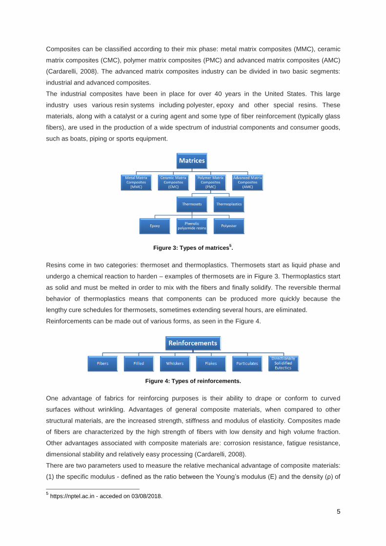
Figure 2: Composite material generic composition.4
Composite materials are usually made of two distinctive phases: matrix and reinforcement - in the
case of Figure 2, the reinforcement are fibers.
1 http://www.look4ward.co.uk/x-files/10-ancient-inventions-you-thought-were-modern/ - acceded on 01/08/2018.
2https://www.liveauctioneers.com/item/63054566_egyptian-ptolemaic-gilt-cartonnage-sarcophagus-mask -
acceded on 01/08/2018 3 http://aerospaceengineeringblog.com/composite-materials/ - acceded on 01/08/2018.
4 https://www.intechopen.com/books/composites-and-their-properties/comparative-review-study-on-elastic-
properties-modeling-for-unidirectional-composite-materials - acceded on 01/08/2018.
5
Composites can be classified according to their mix phase: metal matrix composites (MMC), ceramic
matrix composites (CMC), polymer matrix composites (PMC) and advanced matrix composites (AMC)
(Cardarelli, 2008). The advanced matrix composites industry can be divided in two basic segments:
industrial and advanced composites.
The industrial composites have been in place for over 40 years in the United States. This large
industry uses various resin systems including polyester, epoxy and other special resins. These
materials, along with a catalyst or a curing agent and some type of fiber reinforcement (typically glass
fibers), are used in the production of a wide spectrum of industrial components and consumer goods,
such as boats, piping or sports equipment.
Figure 3: Types of matrices5.
Resins come in two categories: thermoset and thermoplastics. Thermosets start as liquid phase and
undergo a chemical reaction to harden – examples of thermosets are in Figure 3. Thermoplastics start
as solid and must be melted in order to mix with the fibers and finally solidify. The reversible thermal
behavior of thermoplastics means that components can be produced more quickly because the
lengthy cure schedules for thermosets, sometimes extending several hours, are eliminated.
Reinforcements can be made out of various forms, as seen in the Figure 4.
Figure 4: Types of reinforcements.
One advantage of fabrics for reinforcing purposes is their ability to drape or conform to curved
surfaces without wrinkling. Advantages of general composite materials, when compared to other
structural materials, are the increased strength, stiffness and modulus of elasticity. Composites made
of fibers are characterized by the high strength of fibers with low density and high volume fraction.
Other advantages associated with composite materials are: corrosion resistance, fatigue resistance,
dimensional stability and relatively easy processing (Cardarelli, 2008).
There are two parameters used to measure the relative mechanical advantage of composite materials:
(1) the specific modulus - defined as the ratio between the Young’s modulus (E) and the density (ρ) of
5 https://nptel.ac.in - acceded on 03/08/2018.
6
the material and (2) the specific strength - defined as the ratio between the strength (σult) and the
density of the material (ρ):
( )
( )
The combination of these two ratios is known as structural efficiency (Aerospace Structures @ UNSW,
2014). Both ratios are usually higher in composite materials than in monolithic materials. For example,
the strength of a graphite/epoxy unidirectional composite is the same as steel, but the specific strength
is three times higher than steel (Kaw, 1997).
2.2 Composite Materials in the Aeronautical Industry
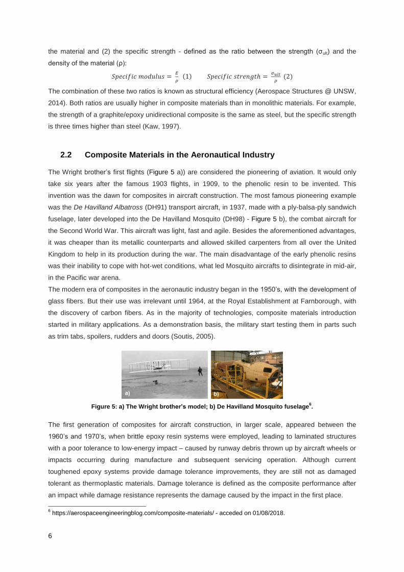
The Wright brother’s first flights (Figure 5 a)) are considered the pioneering of aviation. It would only
take six years after the famous 1903 flights, in 1909, to the phenolic resin to be invented. This
invention was the dawn for composites in aircraft construction. The most famous pioneering example
was the De Havilland Albatross (DH91) transport aircraft, in 1937, made with a ply-balsa-ply sandwich
fuselage, later developed into the De Havilland Mosquito (DH98) - Figure 5 b), the combat aircraft for
the Second World War. This aircraft was light, fast and agile. Besides the aforementioned advantages,
it was cheaper than its metallic counterparts and allowed skilled carpenters from all over the United
Kingdom to help in its production during the war. The main disadvantage of the early phenolic resins
was their inability to cope with hot-wet conditions, what led Mosquito aircrafts to disintegrate in mid-air,
in the Pacific war arena.
The modern era of composites in the aeronautic industry began in the 1950’s, with the development of
glass fibers. But their use was irrelevant until 1964, at the Royal Establishment at Farnborough, with
the discovery of carbon fibers. As in the majority of technologies, composite materials introduction
started in military applications. As a demonstration basis, the military start testing them in parts such
as trim tabs, spoilers, rudders and doors (Soutis, 2005).
Figure 5: a) The Wright brother’s model; b) De Havilland Mosquito fuselage6.
The first generation of composites for aircraft construction, in larger scale, appeared between the
1960’s and 1970’s, when brittle epoxy resin systems were employed, leading to laminated structures
with a poor tolerance to low-energy impact – caused by runway debris thrown up by aircraft wheels or
impacts occurring during manufacture and subsequent servicing operation. Although current
toughened epoxy systems provide damage tolerance improvements, they are still not as damaged
tolerant as thermoplastic materials. Damage tolerance is defined as the composite performance after
an impact while damage resistance represents the damage caused by the impact in the first place.
6 https://aerospaceengineeringblog.com/composite-materials/ - acceded on 01/08/2018.

7
One of the most attractive advantages of composite materials in aeronautical applications is the
capability provided to reduce the number of parts required, namely with complex geometries,
particularly through thermoforming (Tanasa & Zanoaga, 2013).
Toughened epoxy — with thermoplastics and reactive rubber compounds added to counteract
brittleness due to high degree of crosslinking — have become the standard in high-percentage
composite airframes, such as the Boeing 787 Dreamliner - Figure 6 - and the Airbus A350 XW -
Figure 7 - (Sloan, 2016). Carbon fiber represents now more than 50% of the structural weight (aircraft
without engines) of the most efficient airplanes flying – Airbus A350 and Boeing 787.
Figure 6: Materials distribution for the Boeing 7877.
The selection of the appropriate fiber depends on the application. For example, in military aircraft both
high modulus and high strength are desirable. Satellite applications, in contrast, benefit from use of
high fiber modulus improving stability and stiffness for reflector dishes, antennas and their supporting
structure (Soutis, 2005).
Regarding newer technologies, Airbus claims it is at the point of a step-change in weight reduction and
efficiency - producing aircraft parts which weigh 30 to 55% less, while reducing raw material used by
90% may be the next industrial revolution (Cognizant, 2015).
Figure 7: Airbus composite structural weight development8.
Conventional epoxy aerospace resins are designed to cure at 120-135 or 180ºC in an autoclave or
close cavity tool at pressures up to 8 bar and occasionally with a post-cure at a higher temperature.
Systems intended for high temperature application (such as skin in space vehicles) may undergo
curing at temperatures up to 350ºC (Soutis, 2005).
7 https://aviation.stackexchange.com/questions/35441/why-are-the-leading-edges-on-the-boeing-787-made-from-
aluminum - acceded on 05/08/2018. 8 http://scribol.com/technology/aviation/airbus-a350-composites-on-trial-part-i/ - acceded on 07/09/2018.

8
The autoclaves used in the aerospace market can measure up to 27 [m] long, 8 [m] wide and weights
in the region of 300 [ton], costing around 6 M€. This value is added to the production costs associated
with the stemming from nitrogen used for filling and the energy consumptions required to heat and
pressurized the entire volume (Witik et al., 2012).
The effort to improve through-the-thickness strength properties and impact resistance moved away the
composites industry from brittle resins and progressed to thermoplastic resins, toughened epoxies,
through damage tolerance methodology, Z-fiber (carbon, steel or titanium pins driven through the z-
direction to improve the through thickness properties), stitched fabrics, stitched performs and the focus
is now affordable processing methods such as out-of-autoclave processes, non-thermal electron beam
curing by radiation and cost effective production. NASA Langley claims a 100% improvement in
damage tolerance performance with stitched fabrics relative to conventional materials (Irving & Soutis,
2015).
The majority of aircraft control-lift surfaces produced has a single degree of curvature due to limitation
of metal production techniques. Improvements in aerodynamic efficiency can be obtained by moving
to double curvature, allowing, for example, the production of variable camber and twisted wings.
Composites and modern mold tools allow the shape to be tailored in order to meet the required
performance targets at various points of the flying envelope. A further benefit is the ability to tailor the
aero-elasticity of the surface for further improves of the aerodynamic performance. This tailoring can
involve the adoption of laminate configurations that allow the cross-coupling of flexure and torsion,
such that wing twist can result from bending and vice-versa.
Carbon Fiber Reinforced Polymers (CFRP) are now more used in aircraft structures than Glass Fiber
Reinforced Polymers (GFRP). Glass Fiber Reinforced Polymers are often chosen for impact sensitive
applications, even though it has lower elastic modulus and resistance to fatigue, when compared to
carbon fiber. In fighter aircraft, the percentage of composite material is in the range of 20–30% (Safri,
Sultan, Yidris, & Mustapha, 2014).
Figure 8: Airbus A380 design criteria (Pora, 2001).
In Figure 8 is possible to understand the different design criteria applied for different aeronautic parts.
The carbon composites for the aerospace and defense industry represented 30% of the global
demand (in tons) and 61% of the global revenue in 2015. Across all industries, an annual growth of 9-
12%, in demand, is expected until 2022 (Kühnel & Kraus, 2016).
Most aerospace composite structures produced today use prepregs and autoclave cure. Recently, an
increasing number and type of large and critical structures are being manufactured in a very different
way – using preforms assembled from dry fabrics and tapes to then infuse the epoxy resin into the

9
preform, followed by cure. If the infusion is performed in a matched closed mold under high pressure,
the process is called RTM. For many larger parts, infusion is performed using vacuum pressure only
with single surface tools. This process has many different designations, reflecting slight differences in
the infusion process including: Vacuum Assisted Resin Transfer Molding (VARTM), Controlled
Atmospheric Pressure Resin Infusion (CAPRI), Airbus-patented Vacuum Assisted resin infusion
Process (VAP), Resin Transfer Injection (RTI) or Resin Film Infusion (RFI).
Figure 9: 787 Dry fiber/infused parts include (left to right) ailerons and flaps, fuselage frames and the aft
pressure bulkhead (APB) of the fuselage (Dry Composites, 2013).
A wide range of aerospace parts are fully qualified and in production today made from dry fiber and
vacuum infusion – examples are described in Figure 9, Figure 10 and Figure 11. Some of these
assemblies, such as flight control surfaces and fuselage frames, are considered secondary or
redundant components. Others, such as the aft pressure bulkheads of the A380 and Boeing 787, are
primary structure – failure of these critical components would likely lead to loss of the aircraft. The
A400 Cargo Door operates in an even more challenging environment – this flat and large door
withstands cabin pressurization and experiences significant bending and tensile loads during flight.
Figure 10: A380 Aft Pressure Bulkhead and A400 pressurized Cargo Door (Dry Composites, 2013).
The use of critical parts produced by these processes demonstrates the high degree of confidence
that the aircraft OEM’s (original equipment manufacturers) and regulatory authorities have in the
reliability, performance and safety of the dry fiber/infusion approach.
Figure 11: The Bombardier C Series wing (left) and Irkut MS21 wing (right) both are made from dry fiber
preforms and resin infusion (Dry Composites, 2013).
Arguably the most advanced use of dry fibers and infusion is in the wings of next generation airliners
such as the Bombardier C Series and Irkut MS21 aircraft - Figure 11. These aircraft, carrying 120 to
200 passengers, are the newest in commercial aviation and have leveraged the latest advances in
composite materials, processes and production methods available today (Dry Composites, 2013).

10
2.3 Production Processes
Composite materials production processes can be divided in different types, depending on the
processes parameters. For the American Composites Manufacturers Association (ACMA), the
processes are divided in three types: open molding, closed molding and cast polymer moldings.
Open molding: the raw materials (resins and fiber reinforcements) are exposed to air as they cure or
harden. Open molding uses different processes, including hand lay-up, spray-up, casting and filament
winding.
Hand lay up: is the most common and least expensive open-molding method, because it requires the
least amount of equipment. Fiber reinforcements are placed by hand in a mold and the resin is applied
with a brush or a roller. This process is used to make both large and small parts, including boats,
storage tanks, tubs and showers. Its most known variation is the wet-layup.
Spray-up: similar to hand lay-up but it requires special equipment, most notably a chopper gun, to cut
reinforcement material into short fibers, add them to resin and then deposit the mixture (called chop)
onto a molding surface. Spray-up is more automated than hand lay-up and is typically used to produce
large quantities.
Filament Winding: an automated process that applies resin-saturated, continuous strands of fiber
reinforcements over a rotating cylindrical mold. It is used for creating hollow products like rocket motor
casings, pipes, stacks and chemical storage tanks. This method is less labour-intense than the other
open-molding processes.
Closed molding: the raw materials (fibers and resin) cure inside a two-sided mold or within a vacuum
bag. Closed molding processes are often automated and require special equipment, meaning they are
mainly used in large plants that produce high volumes of material - up to 500,000 parts a year.
Vacuum Bag Molding - this manufacturing process is designed to improve the mechanical properties
of a laminate. Vacuum is created to force out the trapped air and excess of resin, compacting the
laminate. High-fiber concentration provides more adhesion. In addition, vacuum bag molding allows
the reduction or elimination of resin excess that builds up when structures are made using hand lay-up
techniques (open-molding).
Vacuum Infusion Processing - vacuum infusion processing (VIP) is a technique that uses vacuum
pressure to drive resin into a laminate. Vacuum infusion is typically used to manufacture very large
structures. This method produces strong, lightweight laminates and offers substantial emissions
reductions (compared to open-molding processing and wet lay-up vacuum bagging). This process
uses the same low-cost tooling as open molding and requires minimal equipment.
Resin Transfer Molding - resin transfer molding (RTM), also referred as liquid molding, is a closed-
molding method in which the reinforcement material is loaded into a closed mold. The mold is then
clamped and the resin is pumped in (through injection ports), under pressure. This process allows the
production of complex parts with smooth finishes on all exposed surfaces and can be a simple or a
highly automated. By laying up reinforcement dry material inside the mold, any combination of
materials and orientation can be used, including 3-D reinforcements.
Compression Molding - is a manufacturing process in which composite materials are ―sandwiched‖
between two matching molds under intense pressure and temperature (from 120° to 205° C) until the
11
part cures. This technique can be automated and is used to rapidly cure large quantities of complex
fiberglass-reinforced polymer parts. Compression molding features fast molding cycles and high part
uniformity. In addition, labour costs are reduced and it provides design flexibility plus high quality
surface finishes.
Pultrusion - used to form composites into long and consistent shapes, such as rods or bars.
Continuous strands of reinforcement are pulled through a resin bath to saturate them and then pulled
through heated steel molds that sculpt the composites into continuous lengths. The process works
continuously, meaning it can be readily automated, with reduced labour costs. Some applications are:
beams, channels, pipes, tubing, fishing rods and golf club shafts.
Reinforced Reaction Injection Molding - reinforced reaction injection molding (RRIM) is widely used to
produce external and internal automotive parts. In this process, two (or more) resins are heated
separately and combined with milled glass fibers. The mixture is injected into a mold under high
pressure and is compressed, where the resin cures quickly. RRIM composites feature many
processing advantages, including reduced cycle times, reduced labour, reduced mold-clamping
pressure and scrap rate. The RRIM process requires special resins and reinforcements.
Centrifugal Casting – in this process the reinforcements and resin are deposited against the inside
surface of a rotating mold. Centrifugal force holds them in place until the material cures or hardens.
The process is used to produce hollow parts and it is especially suited for producing structures with
large diameters, such as pipes for oil and chemical industry installations and chemical storage tanks.
Continuous Lamination - used to make flat or corrugated sheets and panels for products used in truck
and sidewalls, road signs, skylights, building panels and electrical insulating materials. The process is
highly automated, in which the fibers and resin are combined, sandwiched between two plastic carrier
films and guided through a conveyor process. Forming rollers shape the sheets and the resin is cured
(in an oven or heating zone) to form the composite panel. Panels are automatically trimmed to the
desired width and length.
Cast polymers moldings - are unique in the composites industry: typically don’t have fiber
reinforcement and are designed to meet specific strength requirements of a given application. This
process can produce parts of any shape or size.
Gel coated cultured stone molding - a specialized polyester resin that is formulated to provide a
cosmetic outer surface on a composite product, and to provide weather-ability for outdoor products.
Gel coat consists of a base resin and additives.
Solid surface molding - also known as densified products, consists of a cast matrix without a gel-
coated surface. A vacuum system can be used to remove entrapped air in the matrix. Solid surface
products offer limitless design styles.

12
2.4 Mechanical Tests
There are several mechanical tests for composite materials available in the literature. A table with
standardized mechanical tests is presented in the annex A, as well as tables with references to
documents regarding composites terminology, common practices and guides. In order to select the
mechanical tests to be applied in this work, an overview of literature was addressed bearing in mind
the work objectives.
In (Ribbans, 2015) it is concluded that, despite studies have been developed regarding helical
9structures, there is a lack of studies about the interlaminar shear behavior and the assessment of
their mechanical performance under shear and normal stresses. Furthermore, the crack mechanisms
between the fiber layers of helicoidal structures are not well understood.
Impact is remarkably known as the most severe threat to composite structures during in-service life
(Moura, Morais, & Magalhães, 2005). According to Reid and Zhou, as cited in (Perez, Gil, & Oller,
2011), the poor impact damage tolerance of CFRP is related to 1) low transverse and interlaminar
shear strength; 2) laminar construction to compensate the anisotropic nature of the plies and 3) lack of
plastic deformation. Impact damage on aircrafts can result from: 1) maintenance damage or dropped
tools (less than 10 m/s) - Figure 12 a) ; 2) hail (can reach impact velocities of 60 m/s on the ground
and in the order of hundreds of meters per second in flight); 3) runway debris (in the order of 60 m/s) -
Figure 12 b); 4) collisions between service cars or cargo and the structure (low velocity); 5) bird strikes
- Figure 12 c); 6) ice accumulated in the propellers striking the fuselage; 7) engine or other part debris
and 8) ballistic impact (for military aircraft). Three of these situations are exemplified - Figure 12.
Figure 12: a) Aircraft maintenance10
; b) debris impact11
; c) bird-strike12
.
Maintenance damage or dropped tools: during maintenance impact is a dangerous event,
especially if not immediately reported and assessed. The impacted area may be hardly seen and can
drastically decrease the mechanical properties of the part, such as compression, bending, shear and
fatigue (Moura et al., 2005). Studies performed almost 40 years ago showed that the property which is
most affected after impact is the compression strength, evaluated by the compression after impact
(CAI) test, this property can be decreased by 60%, due fundamentally to the delaminations
propagated (Rhodes, 1980).
9 A helix is a single coil that travels longitudinally while advancing at a fixed distance around a central axis. A
spiral is a curve that originates at a single point and progressively travels further from the central point as it rotates from the origin. A helicoid is a system of successive layers of fibers, rotated by relatively small angles (Ribbans, 2015). Helical represents the shape of a helix while helicoid is having the form of a flattened helix. 10
https://www.latchways.com/wingrip - acceded on 03/08/2018. 11
http://www.afcent.af.mil/Units/379th-Air-Expeditionary-Wing/News/Display/Article/351117/fighting-the-war-on-terror-one-rock-at-a-time/ - acceded on 03/08/2018. 12
https://www.airliners.net - acceded on 03/08/2018.
13
It was reported that at least 13% of six hundred and eighty eight repairs to seventy-one Boeing 747
fuselages were related to impact damage. In the same report was concluded that impact damage is
usually located around the doors, on the nose of the aircraft, in the cargo compartments and at the tail
- due to tail-strikes, as cited in (Safri et al., 2014).
Debris: not all debris can be found in the runway or taxi-way – these ones are known as Foreign
Object Damage or Debris (FOD).
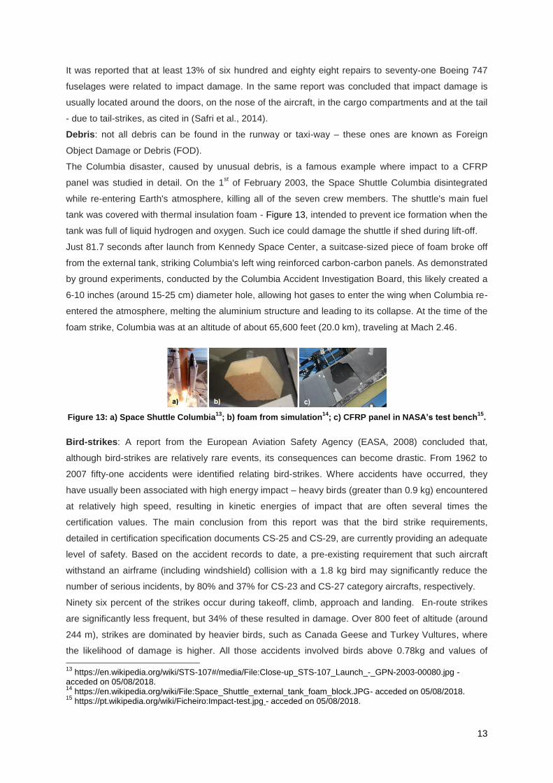
The Columbia disaster, caused by unusual debris, is a famous example where impact to a CFRP
panel was studied in detail. On the 1st of February 2003, the Space Shuttle Columbia disintegrated
while re-entering Earth's atmosphere, killing all of the seven crew members. The shuttle's main fuel
tank was covered with thermal insulation foam - Figure 13, intended to prevent ice formation when the
tank was full of liquid hydrogen and oxygen. Such ice could damage the shuttle if shed during lift-off.
Just 81.7 seconds after launch from Kennedy Space Center, a suitcase-sized piece of foam broke off
from the external tank, striking Columbia's left wing reinforced carbon-carbon panels. As demonstrated
by ground experiments, conducted by the Columbia Accident Investigation Board, this likely created a
6-10 inches (around 15-25 cm) diameter hole, allowing hot gases to enter the wing when Columbia re-
entered the atmosphere, melting the aluminium structure and leading to its collapse. At the time of the
foam strike, Columbia was at an altitude of about 65,600 feet (20.0 km), traveling at Mach 2.46.
Figure 13: a) Space Shuttle Columbia13
; b) foam from simulation14
; c) CFRP panel in NASA’s test bench15
.
Bird-strikes: A report from the European Aviation Safety Agency (EASA, 2008) concluded that,
although bird-strikes are relatively rare events, its consequences can become drastic. From 1962 to
2007 fifty-one accidents were identified relating bird-strikes. Where accidents have occurred, they
have usually been associated with high energy impact – heavy birds (greater than 0.9 kg) encountered
at relatively high speed, resulting in kinetic energies of impact that are often several times the
certification values. The main conclusion from this report was that the bird strike requirements,
detailed in certification specification documents CS-25 and CS-29, are currently providing an adequate
level of safety. Based on the accident records to date, a pre-existing requirement that such aircraft
withstand an airframe (including windshield) collision with a 1.8 kg bird may significantly reduce the
number of serious incidents, by 80% and 37% for CS-23 and CS-27 category aircrafts, respectively.
Ninety six percent of the strikes occur during takeoff, climb, approach and landing. En-route strikes
are significantly less frequent, but 34% of these resulted in damage. Over 800 feet of altitude (around
244 m), strikes are dominated by heavier birds, such as Canada Geese and Turkey Vultures, where
the likelihood of damage is higher. All those accidents involved birds above 0.78kg and values of
13
https://en.wikipedia.org/wiki/STS-107#/media/File:Close-up_STS-107_Launch_-_GPN-2003-00080.jpg - acceded on 05/08/2018. 14
https://en.wikipedia.org/wiki/File:Space_Shuttle_external_tank_foam_block.JPG- acceded on 05/08/2018. 15
https://pt.wikipedia.org/wiki/Ficheiro:Impact-test.jpg - acceded on 05/08/2018.

14
kinetic energy well above current certification values - 90% of the accidents involved impact kinetic
energies above 1500 J. For fixed wing aircraft with certification requirements, the few accidents that
have occurred in these conditions were in the range 2.7 to 6.6 times the certification value.
Twenty eight percent of the strikes reported involved multiple birds, and for these the likelihood of
damage resulting was approximately twice that for an equivalent single strike. Neither the FAA nor
EASA non-engine regulations currently contain any requirements relating to multiple bird strikes of the
type that may arise from bird flocking behavior. Such multiple strikes may result in some pre-loading
of the aircraft structure and windshields, meaning that the current certification analysis and test
regimes are inadequate to model this scenario.
The aircraft parts most likely to be damaged are the nose, radome, fuselage and the wings.
For EASA, kinetic energy is a better indicator of damage likelihood than bird mass. The proportion of
strikes with kinetic energy above the certification value appears to be a useful safety indicator. The
current value for CS-25 aircraft is around 0.3% (EASA, 2008).
Mechanical tests to be performed
From the mechanical tests for composite materials presented, and considering the above mentioned,
three will be employed in this work:
● Tensile – the primary test for materials characterization;
● ILSS – for the evaluation of interlaminar shear strength – a key factor in the process of delamination;
● Impact – to compare the impact behavior of laminates with different stacking sequences.
2.4.1 Introduction to Failure Modes
Failure in composite materials seldom occurs catastrophically and without warning, but tends to be
progressive, with substantial damage widely dispersed through the material. Different mechanical
solicitations in a composite part can induce different failure modes. The combination of these
processes develops a widespread damage through the bulk of the composite and leads to a
permanent degradation in mechanical properties, notably stiffness and residual strength. Some of
these failure modes are presented in Figure 14.
Figure 14: Possible failure modes in composites – as illustrated in (Safri et al.,2014).
Tensile loading can produce: matrix cracking, fiber bridging, fiber pull-out, interfacial (fiber/matrix)
debonding and fiber rupture or breakage.
For the interlaminar shear strength test, the typical failure modes, in accordance with (ASTM
D2344, 2000), are: interlaminar shear - promoting delamination, flexure - that can include micro-
cracking and inelastic deformation.
During impact events, internal damage is formed in the composite laminates and expands around the
impact area, reducing the composite stiffness and strength. Most of the kinetic energy of the projectile
is expended in the plastic deformation of the target material before perforation. The three most
common failure modes in composites subjected to low velocity impact loading are described:
15
- Matrix cracking: is considered the first type of failure caused by low-velocity impact and
occurs parallel to the fibers due to tension, compression and shearing. It can decrease the
interlaminar shear and compression strength properties on the resin or the fiber/resin
interface. Micro-cracking can have a negative effect on a high temperature resin’s properties;
- Delamination: the most critical damage mechanism in composites for low velocity impacts -
due to the fact it can dramatically reduce the post-impact compressive strength of the laminate
and because is not visible to the naked eye. Delaminations are formed between the layers of
the laminate and may be initiated by matrix cracks when threshold energy has been reached.
This failure mode is frequently generated in composite laminates due to out-of-plane impacts.
Delamination may also originate during the manufacturing stage due to the shrinkage of the
matrix during curing or due to the formation of resin-rich areas that result from poor practices
when laying the plies (Travesa, 2006). The shape of delamination is usually that of an oblong
peanut, where (Olsson & Davies, 2004) cited the major axis follows the orientation of the lower
ply at the interface. The oblong peanut shape results from the shear stress distribution around
the neighbouring area of the impactor with low interlaminar shear strength along or close to
the direction of the fibers and of the matrix cracks created by the flexural in-plane stresses
(Davies & Zhang, 1995);
- Fiber Failure: fiber pull-out and fiber breakage are the most common failures under low
velocity impact testing. Fiber failure occurs due to the high stress field and indentation effects.
The projectile induces a shear force and high bending stresses in the non-impacted side of the
specimen.
There is no consensus regarding impact categories. Different authors divide impact categories
differently. For example, as cited in the (Moura et al., 2005), three different studies - (Wang & Yew,
1990); (Sjoblom, Hartness, & Codell, 1988) and (Abrate, 1991) – divide the impact in two categories
regarding impact velocity: 1) Low Velocity Impact – characterized by an extended damage zone and a
global structural response; and 2) High Velocity Impact – characterized by a transient solicitation,
leading to a localized response, with or without perforation. In another study (Safri et al., 2014) the
hyper velocity concept is introduced - low velocity impacts occur at velocities below 10 m/s,
intermediate impacts occur between 10 m/s and 50 m/s, high velocity (ballistic) impacts are within a
range of velocity from 50 m/s to 1000 m/s and hyper velocity impacts have the range of 2-5 km/s.
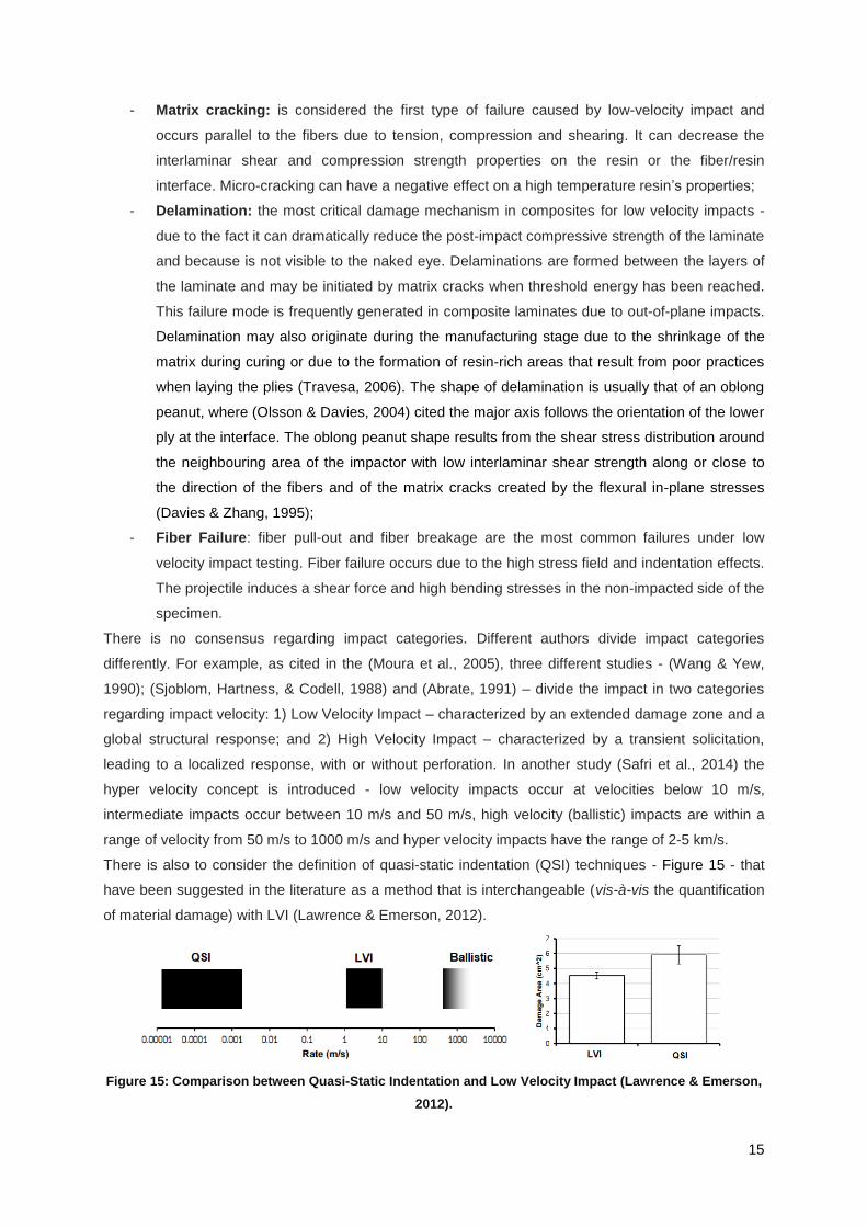
There is also to consider the definition of quasi-static indentation (QSI) techniques - Figure 15 - that
have been suggested in the literature as a method that is interchangeable (vis-à-vis the quantification
of material damage) with LVI (Lawrence & Emerson, 2012).
Figure 15: Comparison between Quasi-Static Indentation and Low Velocity Impact (Lawrence & Emerson,
2012).

16
Compared to QSI, material tested under LVI sustains significantly less interlaminar delamination -
Figure 15, as evidenced by the damage area measurements. Furthermore, material tested with LVI
exhibits significant intra-laminar fracture. This change in the material response is manifested by a
moderately increase of the apparent sample stiffness and energy absorption. The fact that both LVI
and QSI result in essentially identical compression-after-impact/indent strengths further shows the
confounding effects of different damage modes on the apparent damage tolerance of this material
system (Lawrence & Emerson, 2012) and (Feraboli, Ireland, & Kedward, 2004). Besides impact
velocity, other parameters shall be considered, such as the shape of the impactor or its mass, for a
given energy level.
2.5 Non-Destructive Techniques (NDT)
Since destructive tests, as the impact test ASTM D7136 or the compression after impact test ASTM
D7137, involve high costs due to the destruction of the specimen and considering the need of
evaluating in-service composite structures, non-destructive techniques have been extensively
developed and applied throughout the years.
Due to the anisotropic nature of composites, which properties depend on the directions of the
reinforcements, the identification of damage requires NDT techniques to be carried out by qualified
personnel according to EN4179 standard (under EASA) or in accordance with MIL-STD-410 (under
the FAA – Federal Aviation Administration). These techniques are based on different methodologies.16
Non-destructive techniques may also involve considerable costs, but they pay-off in the long term for
most industries. Advanced non-destructive methods are especially important for carbon fiber, since its
final product is a black fiber, resulting in a more difficult damage assessment when compared to glass
fibers, for example.
The most significant defects in monolithic structures are: the void content (in manufacturing) and the
impact damage (during in-service of the composite part). While impact behavior was already
summarized in 2.4.1, the parameters of void content are: 1) duration of the process; 2) temperature
and 3) pressure applied and 4) resin escape system. Void content affects significantly the ILSS, as
observed in Figure 16.
Imperfections in alignment introduced during the manufacturing process result in complex-shaped
voids. These act as stress raisers and points of weakness leading to a reduction in strength
properties. Other sources of weakness, which are often associated with the manufacturing method,
include surface pits and macro-crystallites (Kennerley, 1998).
Damage to composite structures may not be visible following an impact collision. All impacts must be
reported immediately. For the case of aeronautical structures, a qualified and licensed engineer shall
inspect the impacted area and formally record the assessment in the Aircraft Tech Log or other official
document. Failure to detect or report the damage induced may result in an aircraft getting airborne in
an un-airworthy condition. It is essential to determine the existence and location of the damage (Safri
et al., 2014).
16
https://www.skybrary.aero/index.php/Non_Destructive_Testing_of_Composite_Materials_in_Aviation - acceded on 05/08/2018.

17
Figure 16: Relationship between Interlaminar shear strength and Void Content for unidirectional HTS
carbon fibers in an ERLA 4617 epoxy-resin matrix (source: Stone D. and Clarke B. (1974). Non-destructive
Determination of the Void Content in Carbon Fiber Reinforced Plastics by Measurement of Ultrasonic
Attenuation, RAE Technical Report 74162) – as cited in (Smith, 2009).
A set of non-destructive techniques is summarized:
Optical inspection – a visual observation of the component that may require the use of a lens.
Advanced methods include the reflection of a light wave, holographic techniques and interferometry.
Penetrating liquids - an inspection that allows the identification of open surface discontinuities by
taking advantage of the ability of some liquids to penetrate, by capillarity, in the cavities or emerging
cracks.
Eddy currents - if the composite is electrically conductive, another applicable technique is based on
the use of eddy currents. A sub-surface control is prepared with a probe, where an alternating current
passes through, and it produces eddy currents by electromagnetic induction. This technique allows the
detection of defects located below the outer surface of the component under inspection.
Radiography – this method allows the detection of defects, such as voids or the presence of small
foreign object debris - the irregularities are presented with a different density than the bulk material. X-
ray computerized tomography can offer 3D views of the post-impact damage (González, Maimí,
Camanho, Lopes, & Blanco, 2011).
Thermography - thermal imaging with infrared thermo-cameras detects the temperature of the bodies
analyzed. Defects correspond to changes in temperature, thereby identifying a possible initiation of
cracks.
Acoustic techniques - the defects which are present in the material - for example, cracks and/or
debonding - are detected by means of ultrasonic signals generated by a suitable probe or by means of
acoustic signals generated manually by the operator.
Ultrasound - a particular acoustic method that works by sending continuous waves of sound into the
object and capturing the reflected sounds. The reflected sounds are converted into an image to
estimate the size and shape of the defects. There are different types of ultrasonic testers - from
simple devices that give only a digital readout of the thickness to complex systems that show the size
and shape of the defects (Kessler, 2004).
18
Microwave - works by sending microwaves through the material - these waves are then absorbed into
a thin film, which can be enhanced to display defects in the specimen. The microwave testing
techniques are beneficial in that the air surrounding the composite results in low impedance to the
microwaves. This test can be hazardous, as microwaves may induce health concerns (Kessler,
2004).
Low frequency methods – these methods are necessary when material thickness increases, as in
sandwich structures, since they can go deeper, but losing focal sharpness. In low frequency methods
two categories are considered: global assessment – forcing a vibration in all the structure to determine
its natural frequencies and local assessment – to determine the vibration modes. These low frequency
methods are also included in the general vibration tests that allow a fast and efficient way to determine
failures in a structural element, as well as to characterize and locate the damage vicinity. The
measured change of the natural frequencies can be employed to identify damage, such as
delaminations and those related to the residual properties.
2.6 Bio-inspired Solutions
After recognizing the poor damage tolerance of laminated composite materials in through-the-
thickness direction, strategies have been drawn to minimize this challenge.
Inspiration in nature is nothing new. Solutions we apply today came from our observation of natural
phenomena. Examples can be seen in the way we build aircrafts and on how we store solar energy -
Figure 17.
Figure 17: Bio-inspired solutions.
In chapter 2 of (Meyers, Chen, Lin, & Seki, 2008), an insight on the chronological sequence of the
principal books and articles on biological materials and biomimetism is drawn in tables. In (Ferreira,
Nóvoa, & Marques, 2016), the authors demonstrate a survey on journal articles regarding
multifunctional composite structures or materials where an increase is observed - Figure 18.
Figure 18: Literature survey on journal articles related to multifunctional composites/structures or
materials (Ferreira et al., 2016).

19
As observed in (Wegst & Ashby, 2004), natural materials are composites comprised of rather limited
selection of constituents such as collagen, keratin and fibroin proteins.
These natural composites are made of biological structures with complex hierarchical architectures,
varying in mechanical properties, from harder to softer structures, and scale, from macro to the nano-
scale. This complexity makes it challenging to replicate these structures synthetically.
It took hundreds of millions of years of evolution to some of these natural structures acquire the
multifunctional properties we try to understand and replicate. For example, the dermal armour present
in fish (e.g. Arapaima gigas and Coelacanth), reptiles (e.g. crocodilian and squamata), and mammals
(e.g. armadillo and pangolin) - (Ginzburg, Pinto, Iervolino, & Meo, 2016).
The hierarchical structures with collagen fibers link rigid scales in order to achieve enhanced flexibility
while maintaining strength properties. These structures are multifunctional since different functions are
accomplished simultaneously, such as: body protection, thermal regulation, coloration for supressing
intra-species recognition and decreasing hydrodynamic drag in fish (Luz & Mano, 2009).
We, as humans, can be also considered as a high performance composite material – with the
examples of ours bones and muscle tissue - that is a multidirectional fibrous laminate (Halpin, 1992).
Besides the multifunctional capabilities, these biological structures possess the mechanical
parameters that make composite materials attractive: low density or weight, high strength, ability to
absorb energy and adapt the shape to respond to different mechanical solicitations. For example,
scales of fish are typically comprised of the combination of a rigid protective external layer with a
flexible internal one, providing mobility and effective load distribution (Ginzburg et al., 2016).
Recapping the objective of improved damage resistance, we look at biological structures where this
capability is notorious.
Yves Bouligand (1935-2011) carried out extensive studies on biological structures, as crab shells, and
demonstrated the existence of twisted morphologies in various Crustaceans by observing the bow/arc-
shaped fibrous patterns using electron and light microscopy - Figure 19.
Figure 19: Hierarchy of crab exoskeleton – adapted from (Meyers et al., 2008).

20
While examining the transverse cross-sections of the structures, Bouligand concluded that the periodic
patterns are in fact formed by stacked laminae of aligned fibers, with each layer rotated by a small
angle relative to the previous one producing a twisted (helicoidal) arrangement (Ginzburg et al., 2016).
From the biological systems that reveal a twisted laminated structure, one of the most fascinating is
the Mantis Shrimp or stomatopods (Odontodactylus scyllarus), which is an ancient member of an
order of crustaceans, Stomatopoda. There are about 400 species of Mantis Shrimp worldwide –
mostly in tropical and sub-tropical waters in the Indian and Pacific Oceans eastern Africa and Hawaii,
hidden in rock formations. Mantis shrimp usually grows to about 10 cm in length, but some species
can reach up to 40 cm. The Peacock Mantis Shrimp is especially known for its dactyl clubs, in blue
color of Figure 20 a), with enhanced damage tolerance.
Figure 20: a) Odontodactylus scyllarus - also known as mantis shrimp; b) Peacock mantis shrimp striking
a shell17
.
These dactyl clubs withstand thousands of high velocity and accelerations (over 20 m/s and 105 m/s2,
respectively) strikes on sea shells and other prey on which they feed (Patek & Caldwell, 2005).
They are composed of oriented crystalline hydroxyapatite and amorphous calcium phosphate,
arranged into an expanded helicoidal organization containing fibrillar chitinous organic matrix. This
structure prevents catastrophic failure during repetitive high-energy loading events, exceeding 200 N
of force in the case of the peacock mantis shrimp (Weaver, et al., 2012) and observed in Figure 21.
The duration of the impact is so brief that more than 100 of these strikes could fit within one blink of a
human eye. And while humans need to use a robust hammer-blow to break shells, these small
crustaceans can fracture it with raptorial appendages, smaller than a child’s pinky finger. To achieve
the impressive accelerations, the Mantis shrimp possess a spring and latch mechanism. As a
consequence of the acceleration involved in the strike, vapor-filled bubbles between the mantis shrimp
clubs and their prey are formed – known as cavitation bubbles. The collapse of these bubbles
produces additional forces induced to the prey.
Regarding the difference of mechanical properties in the thickness direction, the club is comprised of
two main phases: 1) a hard impact region (about 1 mm thick) exhibiting high Young’s modulus and
high strength; and 2) a periodical helicoidal region (2-3 mm thick) of much lower and oscillating
modulus of elasticity (Weaver, et al., 2012). This second region constitutes what is known as a
Bouligand structure. (Weaver, et al., 2012) also explained that the combination of the two-phase
organisation is effective in arresting the crack-propagation when subjected to impact. When the crack
17
https://www.americanscientist.org/article/the-most-powerful-movements-in-biology - acceded on 28/08/2018.
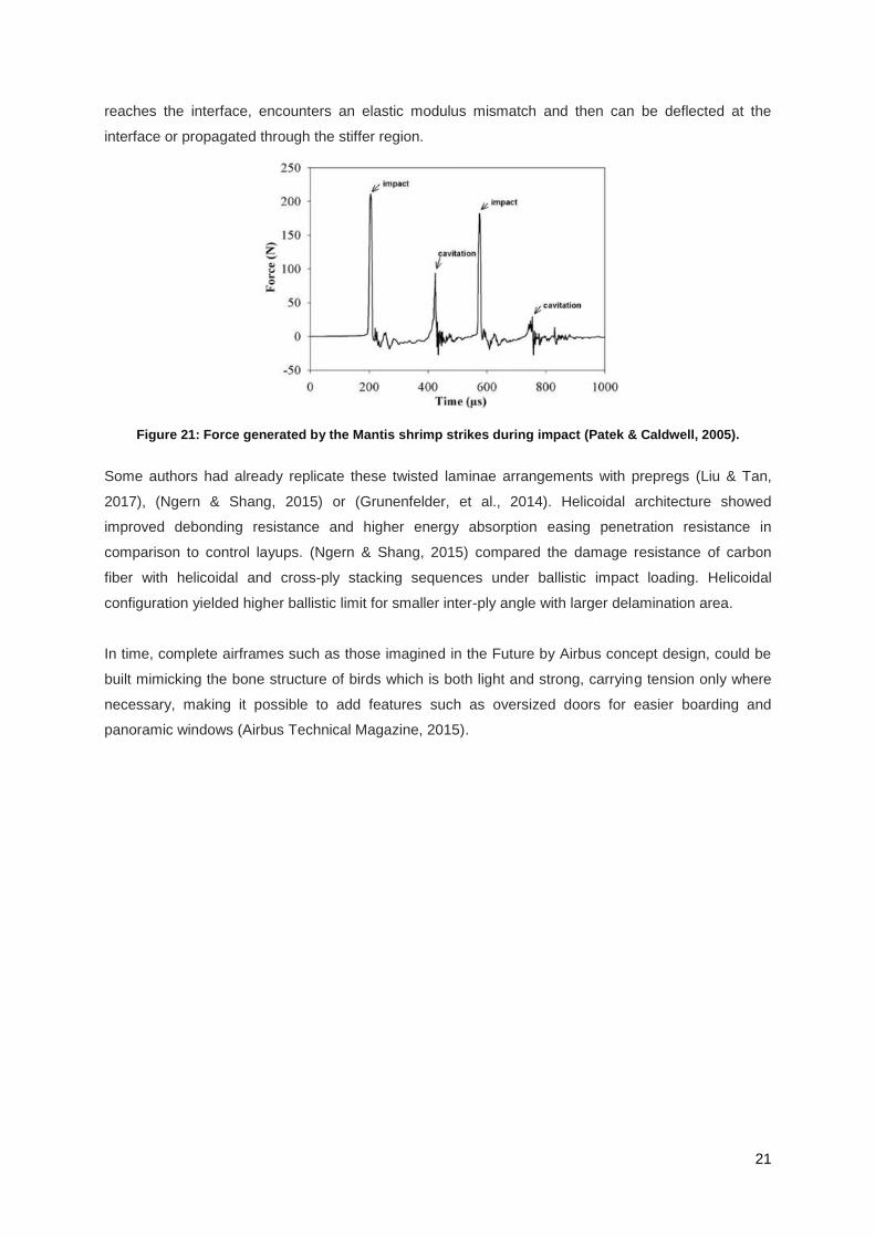
21
reaches the interface, encounters an elastic modulus mismatch and then can be deflected at the
interface or propagated through the stiffer region.
Figure 21: Force generated by the Mantis shrimp strikes during impact (Patek & Caldwell, 2005).
Some authors had already replicate these twisted laminae arrangements with prepregs (Liu & Tan,
2017), (Ngern & Shang, 2015) or (Grunenfelder, et al., 2014). Helicoidal architecture showed
improved debonding resistance and higher energy absorption easing penetration resistance in
comparison to control layups. (Ngern & Shang, 2015) compared the damage resistance of carbon
fiber with helicoidal and cross-ply stacking sequences under ballistic impact loading. Helicoidal
configuration yielded higher ballistic limit for smaller inter-ply angle with larger delamination area.
In time, complete airframes such as those imagined in the Future by Airbus concept design, could be
built mimicking the bone structure of birds which is both light and strong, carrying tension only where
necessary, making it possible to add features such as oversized doors for easier boarding and
panoramic windows (Airbus Technical Magazine, 2015).
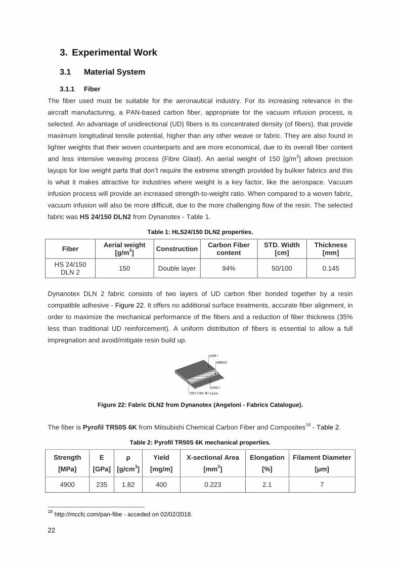
22
3. Experimental Work
3.1 Material System
3.1.1 Fiber
The fiber used must be suitable for the aeronautical industry. For its increasing relevance in the
aircraft manufacturing, a PAN-based carbon fiber, appropriate for the vacuum infusion process, is
selected. An advantage of unidirectional (UD) fibers is its concentrated density (of fibers), that provide
maximum longitudinal tensile potential, higher than any other weave or fabric. They are also found in
lighter weights that their woven counterparts and are more economical, due to its overall fiber content
and less intensive weaving process (Fibre Glast). An aerial weight of 150 [g/m2] allows precision
layups for low weight parts that don’t require the extreme strength provided by bulkier fabrics and this
is what it makes attractive for industries where weight is a key factor, like the aerospace. Vacuum
infusion process will provide an increased strength-to-weight ratio. When compared to a woven fabric,
vacuum infusion will also be more difficult, due to the more challenging flow of the resin. The selected
fabric was HS 24/150 DLN2 from Dynanotex - Table 1.
Table 1: HLS24/150 DLN2 properties.
Fiber Aerial weight
[g/m2]
Construction Carbon Fiber
content STD. Width
[cm] Thickness
[mm]
HS 24/150 DLN 2
150 Double layer 94% 50/100 0.145
Dynanotex DLN 2 fabric consists of two layers of UD carbon fiber bonded together by a resin
compatible adhesive - Figure 22. It offers no additional surface treatments, accurate fiber alignment, in
order to maximize the mechanical performance of the fibers and a reduction of fiber thickness (35%
less than traditional UD reinforcement). A uniform distribution of fibers is essential to allow a full
impregnation and avoid/mitigate resin build up.
Figure 22: Fabric DLN2 from Dynanotex (Angeloni - Fabrics Catalogue).
The fiber is Pyrofil TR50S 6K from Mitsubishi Chemical Carbon Fiber and Composites18
- Table 2.
Table 2: Pyrofil TR50S 6K mechanical properties.
Strength
[MPa]
E
[GPa]
ρ
[g/cm3]
Yield
[mg/m]
X-sectional Area
[mm2]
Elongation
[%]
Filament Diameter
[μm]
4900 235 1.82 400 0.223 2.1 7
18
http://mccfc.com/pan-fibe - acceded on 02/02/2018.

23
3.1.2 Resin
The resin selected was Biresin CR83 with the hardener CH83-6 – mechanical properties in Table 3.
Biresin CR83 is an epoxy resin system with extremely low viscosity and low tendency to crystallise,
designed specifically for the infusion process production of high performance fiber reinforced
composites parts and molds. The system has thermal properties up to 80°C – Table 4, depending on
the cure cycle profile. It is especially suited for use with carbon fiber reinforcement due to its wetting
properties (Sika, 2016). It is important to notice that the values of properties presented by the
manufacturer are obtained with specimens considerably larger than the fine layers of matrix
surrounding the fibers in common laminates (Moura et al., 2005).
Table 3: Resin and hardener mechanical properties.
Typical Mechanical Properties of Fully Cured Neat Resin
Biresin CR83 CH83-6 Test
Tensile strength [MPa] 91
ISO 527 Tensile E-Modulus [MPa] 3200
Elongation at break [%] 8.4
Flexural Strength [MPa] 134 ISO 178
Flexural E-Modulus [MPa] 3360
Compressive strength [MPa] 111 ISO 604
Density [g/cm3] 1.15 ISO 1183
Shore-hardness D85 ISO 868
Impact resistance [kJ/m2] 84 ISO 179
Table 4: Typical Thermal Properties of Fully Cured Neat Resin.
Typical Thermal Properties of Fully Cured Neat Resin
Biresin CR83 CH83-6 Test
Heat distortion temperature [°C] 79 ISO 75B
Glass transition temperature [°C] 80 ISO 11357
Resin’s profile is described by: viscosity, out time, gel time and exothermal rate. The parameters must
be adjusted to the designed application.

24
3.2 Stacking Sequences
An aeronautical standard stacking sequence was provided by Embraer and is represented with the
designation LS. The number of plies was determined in order to the composite panel reaches a
thickness of around 4 [mm], due to the recommendation for the impact test, cited in point 8.2.1 of
(ASTM D7136, 2015), and considering the expected thickness in Table 1.
( )
From the result above, it was decided the number of layers to produce the laminates would be 28.
Bearing in mind the work presented in 2.6, two bio-inspired stacking sequences were selected: a
denominated helicoidal, designated HL, and a helicoidal-symmetric, designated HL-S. Since the
number of layers is known, the angle to perform the helicoidal laminate was calculated:
( )
The helicoidally stacking sequences used were a balanced and a symmetric, with the respective
designations: HL and HL-S - Table 5. The stacking sequences are detailed in Figure 75 (annex B).
Table 5: Laminates stacking sequences.
Designation Description Number of plies Configuration
LS Standard 28 [0/45/90/-45/45/-45/0]2s
HL Helicoidal 28 [0/13.3/26.6/.../360]
HL-S Helicoidal-symmetric 28 [0/13.3/26.6/.../173.3]s
3.3 Production of the laminates
The experimental work was performed in PIEP composites laboratory, in Guimarães.
3.3.1 Unpacking and cutting
The fibers were cutted to the desired orientations. Given the accuracy needed, a laser machine was
used for the cut of the helicoidally stacking sequences.
Figure 23: a) Carbon fiber; b) laser cutting machine.
The parameters to cut the carbon fiber in the laser machine - Figure 23 - were: 95% to 100% of the
available power and a setting speed of about 5% of the maximum achieved by the machine. Even with
these parameters it was further required to cut with a scissor the remaining fibers still attached to the
laminae. The average duration time to cut a 180x550 [mm] panel was 4 minutes. After each cut it was
required to clean the machine’s table with a vacuum cleaner, in order to avoid the deposition of fibers
in the mechanism of the laser machine.
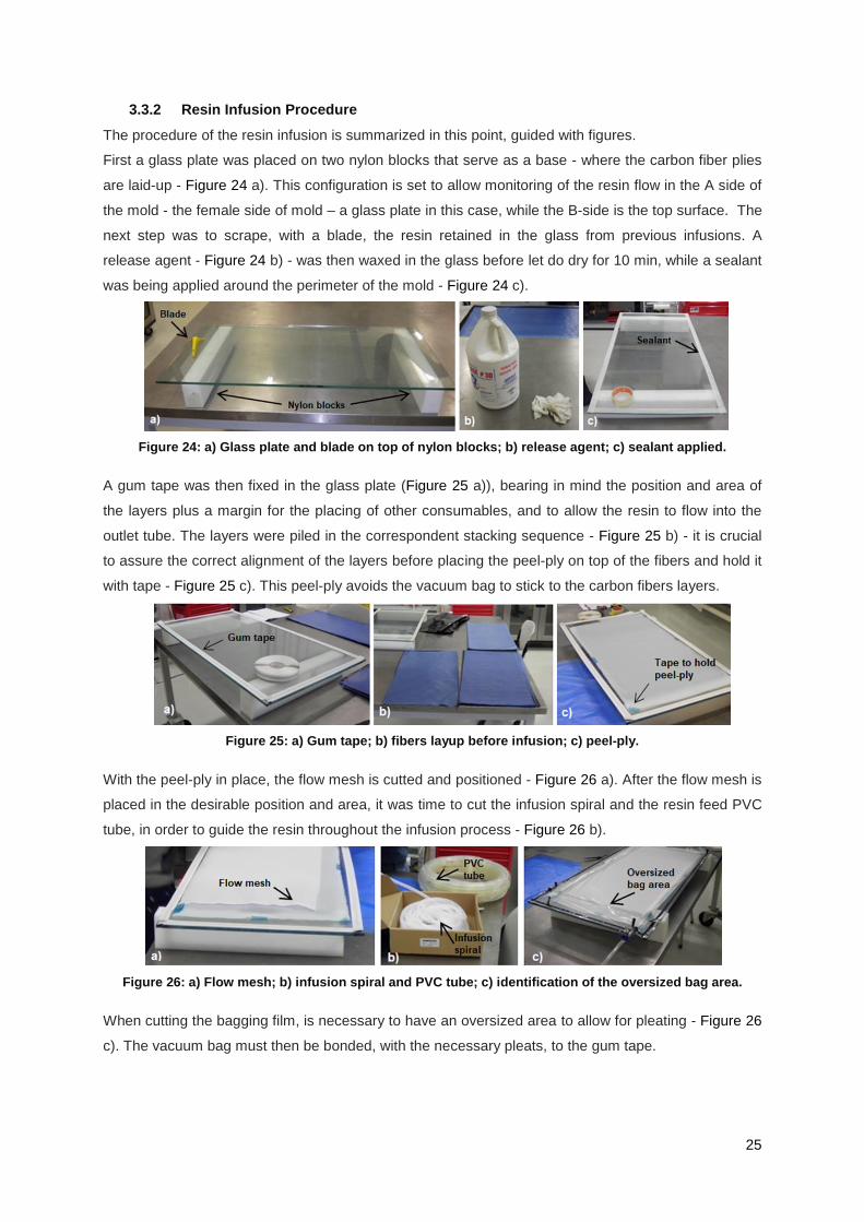
25
3.3.2 Resin Infusion Procedure
The procedure of the resin infusion is summarized in this point, guided with figures.
First a glass plate was placed on two nylon blocks that serve as a base - where the carbon fiber plies
are laid-up - Figure 24 a). This configuration is set to allow monitoring of the resin flow in the A side of
the mold - the female side of mold – a glass plate in this case, while the B-side is the top surface. The
next step was to scrape, with a blade, the resin retained in the glass from previous infusions. A
release agent - Figure 24 b) - was then waxed in the glass before let do dry for 10 min, while a sealant
was being applied around the perimeter of the mold - Figure 24 c).
Figure 24: a) Glass plate and blade on top of nylon blocks; b) release agent; c) sealant applied.
A gum tape was then fixed in the glass plate (Figure 25 a)), bearing in mind the position and area of
the layers plus a margin for the placing of other consumables, and to allow the resin to flow into the
outlet tube. The layers were piled in the correspondent stacking sequence - Figure 25 b) - it is crucial
to assure the correct alignment of the layers before placing the peel-ply on top of the fibers and hold it
with tape - Figure 25 c). This peel-ply avoids the vacuum bag to stick to the carbon fibers layers.
Figure 25: a) Gum tape; b) fibers layup before infusion; c) peel-ply.
With the peel-ply in place, the flow mesh is cutted and positioned - Figure 26 a). After the flow mesh is
placed in the desirable position and area, it was time to cut the infusion spiral and the resin feed PVC
tube, in order to guide the resin throughout the infusion process - Figure 26 b).
Figure 26: a) Flow mesh; b) infusion spiral and PVC tube; c) identification of the oversized bag area.
When cutting the bagging film, is necessary to have an oversized area to allow for pleating - Figure 26
c). The vacuum bag must then be bonded, with the necessary pleats, to the gum tape.
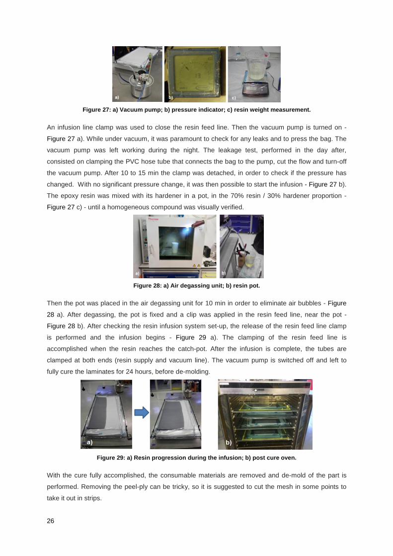
26
Figure 27: a) Vacuum pump; b) pressure indicator; c) resin weight measurement.
An infusion line clamp was used to close the resin feed line. Then the vacuum pump is turned on -
Figure 27 a). While under vacuum, it was paramount to check for any leaks and to press the bag. The
vacuum pump was left working during the night. The leakage test, performed in the day after,
consisted on clamping the PVC hose tube that connects the bag to the pump, cut the flow and turn-off
the vacuum pump. After 10 to 15 min the clamp was detached, in order to check if the pressure has
changed. With no significant pressure change, it was then possible to start the infusion - Figure 27 b).
The epoxy resin was mixed with its hardener in a pot, in the 70% resin / 30% hardener proportion -
Figure 27 c) - until a homogeneous compound was visually verified.
Figure 28: a) Air degassing unit; b) resin pot.
Then the pot was placed in the air degassing unit for 10 min in order to eliminate air bubbles - Figure
28 a). After degassing, the pot is fixed and a clip was applied in the resin feed line, near the pot -
Figure 28 b). After checking the resin infusion system set-up, the release of the resin feed line clamp
is performed and the infusion begins - Figure 29 a). The clamping of the resin feed line is
accomplished when the resin reaches the catch-pot. After the infusion is complete, the tubes are
clamped at both ends (resin supply and vacuum line). The vacuum pump is switched off and left to
fully cure the laminates for 24 hours, before de-molding.
Figure 29: a) Resin progression during the infusion; b) post cure oven.
With the cure fully accomplished, the consumable materials are removed and de-mold of the part is
performed. Removing the peel-ply can be tricky, so it is suggested to cut the mesh in some points to
take it out in strips.
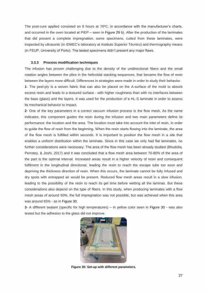
27
The post-cure applied consisted on 8 hours at 70ºC, in accordance with the manufacturer’s charts,
and occurred in the oven located at PIEP – seen in Figure 29 b). After the production of the laminates
that did present a complete impregnation, some specimens, cutted from these laminates, were
inspected by ultrasonic (in IDMEC’s laboratory at Instituto Superior Técnico) and thermography means
(in FEUP, University of Porto). The tested specimens didn’t present any major flaws.
3.3.3 Process modification techniques
The infusion has proven challenging due to the density of the unidirectional fibers and the small
rotation angles between the plies in the helicoidal stacking sequences, that became the flow of resin
between the layers more difficult. Differences in strategies were made in order to study their behavior.
1- The peel-ply is a woven fabric that can also be placed on the A-surface of the mold to absorb
excess resin and leads to a textured surface - with higher roughness than with no interfaces between
the base (glass) and the layers. It was used for the production of a HL-S laminate in order to assess
its mechanical behavior to impact.
2- One of the key parameters in a correct vacuum infusion process is the flow mesh. As the name
indicates, this component guides the resin during the infusion and two main parameters define its
performance: the location and the area. The location must take into account the inlet of resin, in order
to guide the flow of resin from the beginning. When the resin starts flowing into the laminate, the area
of the flow mesh is fulfilled within seconds. It is important to position the flow mesh in a site that
enables a uniform distribution within the laminate. Since in this case we only had flat laminates, no
further considerations were necessary. The area of the flow mesh has been already studied (Bhudolia,
Perrotey, & Joshi, 2017) and it was concluded that a flow mesh area between 70-80% of the area of
the part is the optimal interval. Increased areas result in a higher velocity of resin and consequent
fulfilment in the longitudinal directional, leading the resin to reach the escape tube too soon and
depriving the thickness direction of resin. When this occurs, the laminate cannot be fully infused and
dry spots with entrapped air would be present. Reduced flow mesh areas result in a slow infusion,
leading to the possibility of the resin to reach its gel time before wetting all the laminas. But these
considerations also depend on the type of fibers. In this study, when producing laminates with a flow
mesh areas of around 50%, the full impregnation was not possible, but was achieved when this area
was around 65% - as in Figure 30.
3- A different sealant (specific for high temperatures) – in yellow color seen in Figure 30 - was also
tested but the adhesion to the glass did not improve.
Figure 30: Set-up with different parameters.
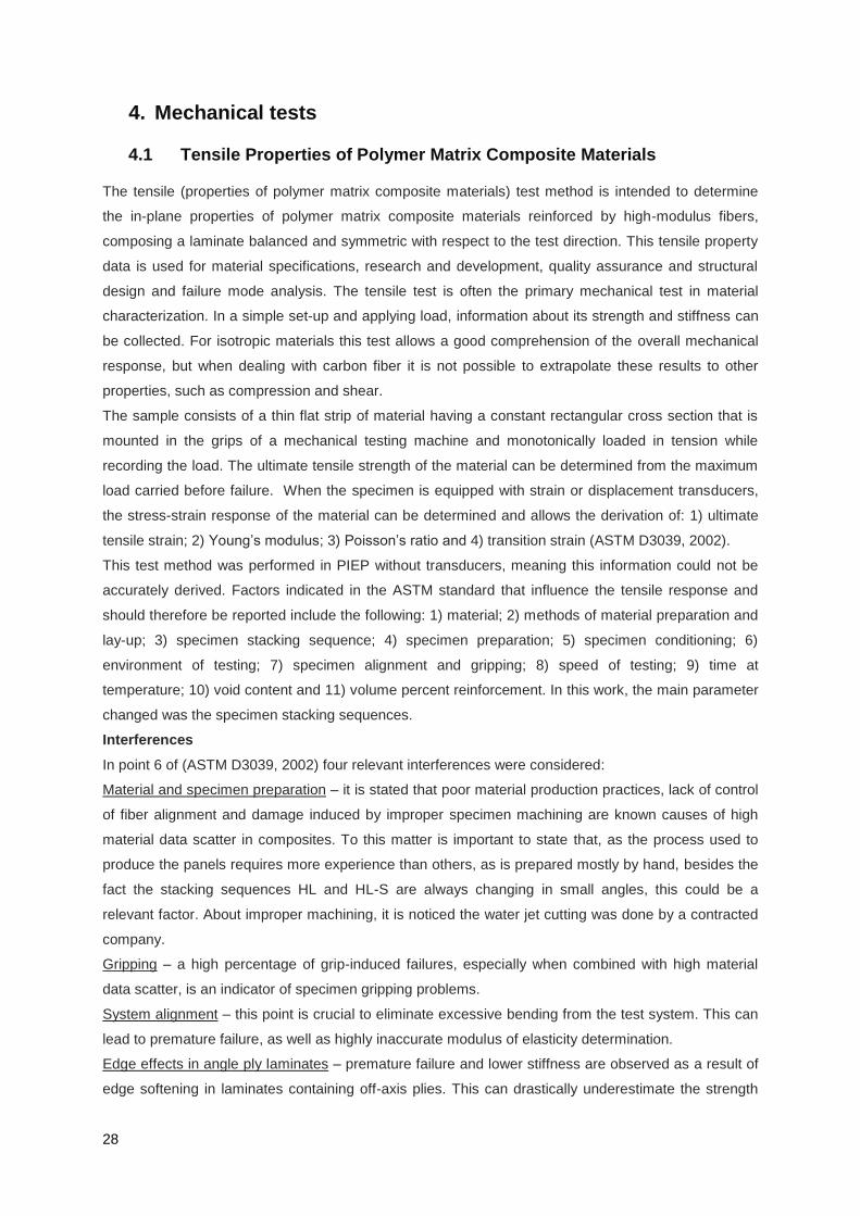
28
4. Mechanical tests
4.1 Tensile Properties of Polymer Matrix Composite Materials
The tensile (properties of polymer matrix composite materials) test method is intended to determine
the in-plane properties of polymer matrix composite materials reinforced by high-modulus fibers,
composing a laminate balanced and symmetric with respect to the test direction. This tensile property
data is used for material specifications, research and development, quality assurance and structural
design and failure mode analysis. The tensile test is often the primary mechanical test in material
characterization. In a simple set-up and applying load, information about its strength and stiffness can
be collected. For isotropic materials this test allows a good comprehension of the overall mechanical
response, but when dealing with carbon fiber it is not possible to extrapolate these results to other
properties, such as compression and shear.
The sample consists of a thin flat strip of material having a constant rectangular cross section that is
mounted in the grips of a mechanical testing machine and monotonically loaded in tension while
recording the load. The ultimate tensile strength of the material can be determined from the maximum
load carried before failure. When the specimen is equipped with strain or displacement transducers,
the stress-strain response of the material can be determined and allows the derivation of: 1) ultimate
tensile strain; 2) Young’s modulus; 3) Poisson’s ratio and 4) transition strain (ASTM D3039, 2002).
This test method was performed in PIEP without transducers, meaning this information could not be
accurately derived. Factors indicated in the ASTM standard that influence the tensile response and
should therefore be reported include the following: 1) material; 2) methods of material preparation and
lay-up; 3) specimen stacking sequence; 4) specimen preparation; 5) specimen conditioning; 6)
environment of testing; 7) specimen alignment and gripping; 8) speed of testing; 9) time at
temperature; 10) void content and 11) volume percent reinforcement. In this work, the main parameter
changed was the specimen stacking sequences.
Interferences
In point 6 of (ASTM D3039, 2002) four relevant interferences were considered:
Material and specimen preparation – it is stated that poor material production practices, lack of control
of fiber alignment and damage induced by improper specimen machining are known causes of high
material data scatter in composites. To this matter is important to state that, as the process used to
produce the panels requires more experience than others, as is prepared mostly by hand, besides the
fact the stacking sequences HL and HL-S are always changing in small angles, this could be a
relevant factor. About improper machining, it is noticed the water jet cutting was done by a contracted
company.
Gripping – a high percentage of grip-induced failures, especially when combined with high material
data scatter, is an indicator of specimen gripping problems.
System alignment – this point is crucial to eliminate excessive bending from the test system. This can
lead to premature failure, as well as highly inaccurate modulus of elasticity determination.
Edge effects in angle ply laminates – premature failure and lower stiffness are observed as a result of
edge softening in laminates containing off-axis plies. This can drastically underestimate the strength
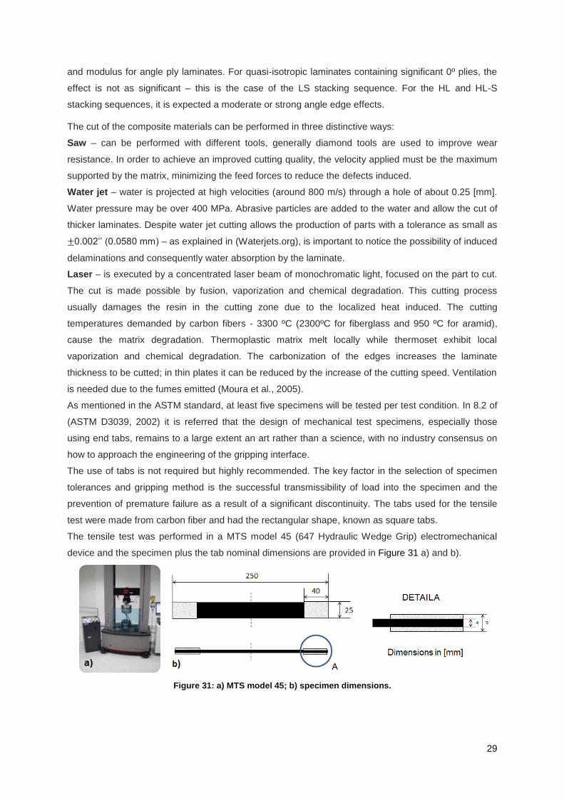
29
and modulus for angle ply laminates. For quasi-isotropic laminates containing significant 0º plies, the
effect is not as significant – this is the case of the LS stacking sequence. For the HL and HL-S
stacking sequences, it is expected a moderate or strong angle edge effects.
The cut of the composite materials can be performed in three distinctive ways:
Saw – can be performed with different tools, generally diamond tools are used to improve wear
resistance. In order to achieve an improved cutting quality, the velocity applied must be the maximum
supported by the matrix, minimizing the feed forces to reduce the defects induced.
Water jet – water is projected at high velocities (around 800 m/s) through a hole of about 0.25 [mm].
Water pressure may be over 400 MPa. Abrasive particles are added to the water and allow the cut of
thicker laminates. Despite water jet cutting allows the production of parts with a tolerance as small as
0.002’’ (0.0580 mm) – as explained in (Waterjets.org), is important to notice the possibility of induced
delaminations and consequently water absorption by the laminate.
Laser – is executed by a concentrated laser beam of monochromatic light, focused on the part to cut.
The cut is made possible by fusion, vaporization and chemical degradation. This cutting process
usually damages the resin in the cutting zone due to the localized heat induced. The cutting
temperatures demanded by carbon fibers - 3300 ºC (2300ºC for fiberglass and 950 ºC for aramid),
cause the matrix degradation. Thermoplastic matrix melt locally while thermoset exhibit local
vaporization and chemical degradation. The carbonization of the edges increases the laminate
thickness to be cutted; in thin plates it can be reduced by the increase of the cutting speed. Ventilation
is needed due to the fumes emitted (Moura et al., 2005).
As mentioned in the ASTM standard, at least five specimens will be tested per test condition. In 8.2 of
(ASTM D3039, 2002) it is referred that the design of mechanical test specimens, especially those
using end tabs, remains to a large extent an art rather than a science, with no industry consensus on
how to approach the engineering of the gripping interface.
The use of tabs is not required but highly recommended. The key factor in the selection of specimen
tolerances and gripping method is the successful transmissibility of load into the specimen and the
prevention of premature failure as a result of a significant discontinuity. The tabs used for the tensile
test were made from carbon fiber and had the rectangular shape, known as square tabs.
The tensile test was performed in a MTS model 45 (647 Hydraulic Wedge Grip) electromechanical
device and the specimen plus the tab nominal dimensions are provided in Figure 31 a) and b).
Figure 31: a) MTS model 45; b) specimen dimensions.

30
For each specimen a caliper rule was used to measure the thickness and width at three locations of
the gage section. The average of three values was considered in order to determine the section area
A = w [mm] x h [mm], width and thickness, respectively. These measurements and calculations are
detailed in tables of the annex C.1. The laboratory atmosphere conditions were in accordance with
ASTM standard (20.9°C and 43.7% of relative humidity). The specimens tested are illustrated in
Figure 32.
Figure 32: Tensile specimens before testing.
In the paragraph 11.3 of it (ASTM D3039, 2002) the speed of testing is considered in order to impose
a nearly constant strain rate at the gage section. If strain control is not available on the testing
machine, it may be approximated by constantly monitoring and adjusting the rate of load application,
as measured by strain transducer response versus time. The strain rate is also selected so failure
occurs within 1 to 10 min. If the ultimate strain of the material cannot be reasonably estimated, initial
trials should be conducted using standard speeds until the ultimate strain of the material and the
compliance of the system are known and the strain rate can be adjusted. The suggested standard
speeds are:
● Strain controlled tests – a standard strain rate of 0.01 [min-1
];
● Constant cross-head speed tests – a standard head displacement of 2 [mm/min].
For this test the standard head displacement of 2 [mm/min] was applied. The importance of a nearly
constant strain rate at the gage section comes from the fact that different strain rates lead to different
strain-rate curves. The specimens were stored and tested in the same laboratory, hence, without
relevant changes of environment (temperature and relative humidity). During the test the load and
cross-head displacement were recorded which enabled the illustration of a load vs. displacement
curve for each specimen.
Parameters Calculations
The ultimate tensile strength is determined by the equation:
( )
Where – ultimate tensile strength [MPa], – maximum load before failure [N] and – average
cross-sectional area [mm2]. The tensile stress is given by:
( )
where – tensile stress at the ith
data point [MPa] and – load at ith
data point [N]. If tensile modulus
or ultimate tensile strain is to be determined and material response is being monitored by a clip gauge,
the tensile strain is determined by the equation:

31
( )
where – tensile strain at ith
data point, – clip gauge displacement at ith data point [mm] and –
clip gauge’s length [mm]. When retrieving the stress-strain data with a clip gauge, the Young’s
modulus of elasticity is determined by the equation:
( )
where – Young’s modulus [GPa], – difference in applied tensile stress between two strain points
[MPa] and – difference between two strain points (nominally 0.002).
As already referred, extensometers weren’t available and therefore the stress-strain curve could not
be presented. For a matter of qualitative comparison, the Young’s modulus was estimated by
assuming the gage length of the specimen for the strain equation. This estimation was performed by
starting at a certain level of strain (0.001) until a specified stress - 100 [MPa], in order to accomplish a
linear and representative region of the curve, for all specimens.
For each series of tests the following terms are determined: average value, standard deviation and
coefficient of variation (in percentage) of each property determined. The equations are, respectively:
(∑
)
( )
√(∑
) ( ) ( )
( ) ( )
To evaluate the failure modes of the specimens, the ASTM standard presents a table with codes to
describe it in terms of failure type, area and location - Table 6.
Table 6: Tensile Test Failure Codes/Typical Modes.
First Character Second Character Third Character
Failure Type Code Failure Area Code Failure Location Code
Angled A Inside grip/tab I Bottom B
edge Delamination D At grip/tab A Top T
Grip/tab G <1/W from grip/tab W Left L
Lateral L Gage G Right R
Multi-mode M Multiple areas M Middle M
long. Spliting S Various V Various V
eXplosive X Unknown U Unknown U
Other O
32
4.2 Interlaminar Shear Strength Test [ILSS]
The interlaminar shear strength test determines the short-beam strength of high-modulus fiber-
reinforced composite materials. This test method is performed to characterize both fiber-matrix
interfacial adhesion and also the effect of binder on the composite mechanical properties (Paiva,
Santos, & Rezende, 2009).
There are two main standards regarding this test method: the (ASTM D2344, 2000) and the (ISO
14130, 1997). The standard (ASTM D2344, 2000) specifies the test for curved or flat laminates up to a
thickness of 6.00 [mm], of continuous or discontinuous fiber-reinforced polymer matrix composites, for
which the elastic properties are balanced and symmetric with respect to the longitudinal axis of the
beam. While the ISO 14130 only refers a bar of rectangular test standard and specifies desirable
specimen’s dimensions, with guidance formulas if the thickness of 2 [mm] may not be achieved.
There is no consensus on how to accurately determine the interlaminar shear strength. Although
shear is the dominant applied loading in the test method, the internal stresses are complex and
different failure modes may occur. As cited in the ASTM 2344, elasticity solutions by (Whitney &
Browning, 1985), and (Sullivan & Van Oene, 1986) have demonstrated inadequacies in classical
beam theory when defining the stress state in the short-beam configuration. These solutions show that
the parabolic shear stress distribution, as predicted by the equation:
( )
only occurs, and then not exactly, on planes midway between the loading nose and support points.
Away from these planes, the stress distributions become skewed, with peak stresses occurring near
the loading nose and support points. Of singular significance is the local stress state around the
loading nose, in which the severe shear-stress concentration combined with transverse and in-plane
compressive stresses have been shown to initiate failure. However, for more ductile matrices, plastic
yielding may mitigate the situation under the loading nose and allows other failure modes to occur,
such as bottom surface fiber tension. Consequently, unless mid-plane interlaminar failure has been
clearly observed, the short-beam strength determined from this test method cannot be attributed to a
shear property, and the use of the equation (12) will not yield an accurate value for shear strength
(ASTM D2344, 2000). This is the reason behind the denomination, used by the standard, of ―apparent‖
interlaminar shear strength. The test method consists of a short-beam specimen center-loaded -
Figure 33.
Figure 33: Loading diagram of the ILSS test - (ISO 14130, 1997).
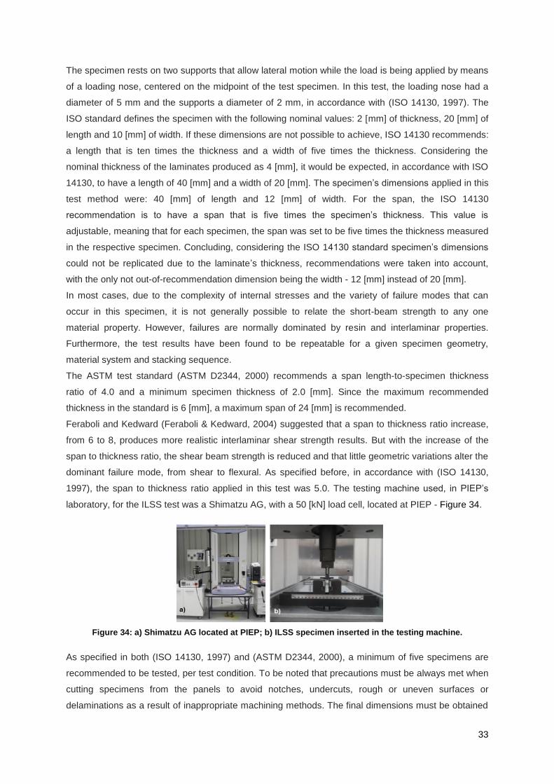
33
The specimen rests on two supports that allow lateral motion while the load is being applied by means
of a loading nose, centered on the midpoint of the test specimen. In this test, the loading nose had a
diameter of 5 mm and the supports a diameter of 2 mm, in accordance with (ISO 14130, 1997). The
ISO standard defines the specimen with the following nominal values: 2 [mm] of thickness, 20 [mm] of
length and 10 [mm] of width. If these dimensions are not possible to achieve, ISO 14130 recommends:
a length that is ten times the thickness and a width of five times the thickness. Considering the
nominal thickness of the laminates produced as 4 [mm], it would be expected, in accordance with ISO
14130, to have a length of 40 [mm] and a width of 20 [mm]. The specimen’s dimensions applied in this
test method were: 40 [mm] of length and 12 [mm] of width. For the span, the ISO 14130
recommendation is to have a span that is five times the specimen’s thickness. This value is
adjustable, meaning that for each specimen, the span was set to be five times the thickness measured
in the respective specimen. Concluding, considering the ISO 14130 standard specimen’s dimensions
could not be replicated due to the laminate’s thickness, recommendations were taken into account,
with the only not out-of-recommendation dimension being the width - 12 [mm] instead of 20 [mm].
In most cases, due to the complexity of internal stresses and the variety of failure modes that can
occur in this specimen, it is not generally possible to relate the short-beam strength to any one
material property. However, failures are normally dominated by resin and interlaminar properties.
Furthermore, the test results have been found to be repeatable for a given specimen geometry,
material system and stacking sequence.
The ASTM test standard (ASTM D2344, 2000) recommends a span length-to-specimen thickness
ratio of 4.0 and a minimum specimen thickness of 2.0 [mm]. Since the maximum recommended
thickness in the standard is 6 [mm], a maximum span of 24 [mm] is recommended.
Feraboli and Kedward (Feraboli & Kedward, 2004) suggested that a span to thickness ratio increase,
from 6 to 8, produces more realistic interlaminar shear strength results. But with the increase of the
span to thickness ratio, the shear beam strength is reduced and that little geometric variations alter the
dominant failure mode, from shear to flexural. As specified before, in accordance with (ISO 14130,
1997), the span to thickness ratio applied in this test was 5.0. The testing machine used, in PIEP’s
laboratory, for the ILSS test was a Shimatzu AG, with a 50 [kN] load cell, located at PIEP - Figure 34.
Figure 34: a) Shimatzu AG located at PIEP; b) ILSS specimen inserted in the testing machine.
As specified in both (ISO 14130, 1997) and (ASTM D2344, 2000), a minimum of five specimens are
recommended to be tested, per test condition. To be noted that precautions must be always met when
cutting specimens from the panels to avoid notches, undercuts, rough or uneven surfaces or
delaminations as a result of inappropriate machining methods. The final dimensions must be obtained

34
by water-lubricated precision sawing, milling or grinding – in order to the edges present the specified
tolerances. The specimens produced in this work were water-lubricated cutted, but with some failures
that didn’t guarantee all the dimensional requirements and therefore, after analyzed in a magnifying
glass, some specimens were rejected - Figure 35.
Figure 35: Example of specimen being examined in the magnifying glass.
Laboratory atmospheric conditions were the same as in 4.1 and the speed of testing applied, of the
crosshead movement, was 1.0 [mm/min]. The specimens were aligned and centered such that its
longitudinal axis was perpendicular to the loading nose and side supports.
Then, for each series of test methods, the average value was determined, as the standard deviation
and the coefficient of variation (in percentage), expressed by eq. (9), (10) and (11), respectively.
In order to validate the interlaminar shear strength test, the failure mode observed must be reported.
The failure modes specified in the standard (ASTM D2344, 2000) are illustrated in Figure 36.
Figure 36: ASTM D2344 failure modes.
4.3 Impact Test
The impact test standardized by ASTM - (ASTM D7136, 2015) - determines the damage resistance of
multidirectional polymer matrix composite laminated plates subjected to an out-of-plane and
concentrated drop-weight impact event (ASTM D7136, 2015). The impact test was performed at PIEP
laboratory, in Guimarães. The testing machine was a Factovis Plus with a range of 21800 [N], from
CEAST - Figure 37.
Figure 37: Fractovis Plus from CEAST and the representation of the strain gauge striker.
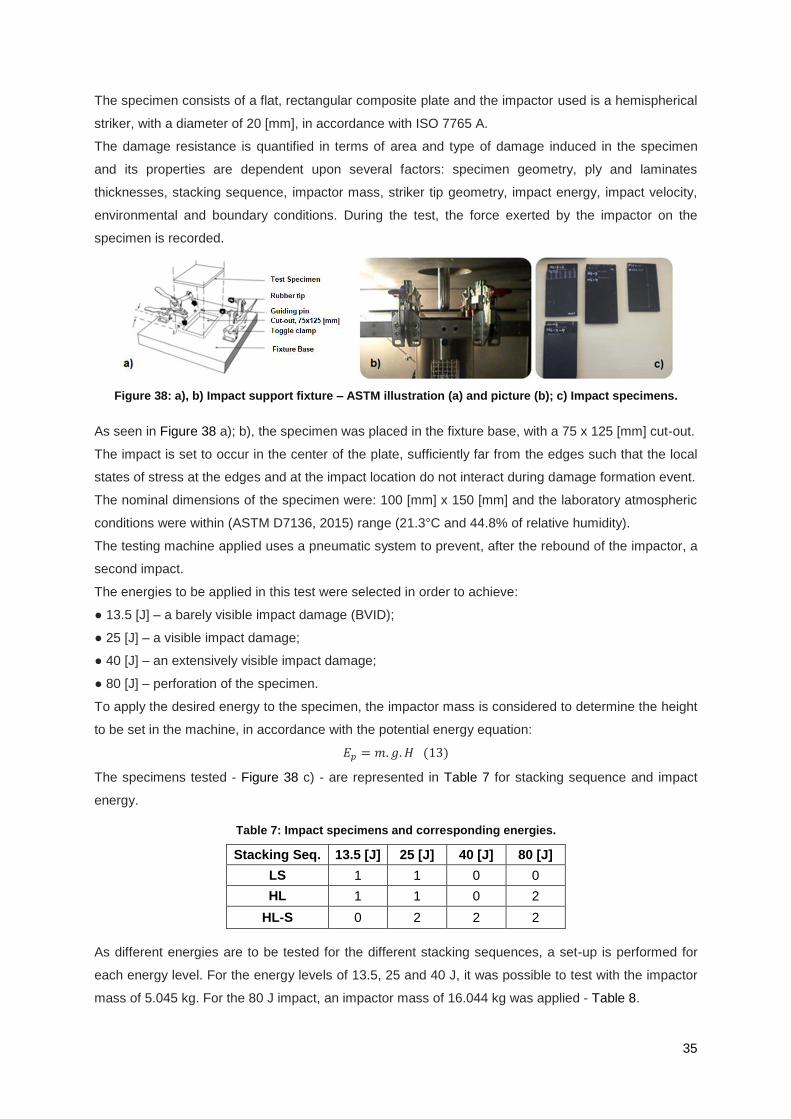
35
The specimen consists of a flat, rectangular composite plate and the impactor used is a hemispherical
striker, with a diameter of 20 [mm], in accordance with ISO 7765 A.
The damage resistance is quantified in terms of area and type of damage induced in the specimen
and its properties are dependent upon several factors: specimen geometry, ply and laminates
thicknesses, stacking sequence, impactor mass, striker tip geometry, impact energy, impact velocity,
environmental and boundary conditions. During the test, the force exerted by the impactor on the
specimen is recorded.
Figure 38: a), b) Impact support fixture – ASTM illustration (a) and picture (b); c) Impact specimens.
As seen in Figure 38 a); b), the specimen was placed in the fixture base, with a 75 x 125 [mm] cut-out.
The impact is set to occur in the center of the plate, sufficiently far from the edges such that the local
states of stress at the edges and at the impact location do not interact during damage formation event.
The nominal dimensions of the specimen were: 100 [mm] x 150 [mm] and the laboratory atmospheric
conditions were within (ASTM D7136, 2015) range (21.3°C and 44.8% of relative humidity).
The testing machine applied uses a pneumatic system to prevent, after the rebound of the impactor, a
second impact.
The energies to be applied in this test were selected in order to achieve:
● 13.5 [J] – a barely visible impact damage (BVID);
● 25 [J] – a visible impact damage;
● 40 [J] – an extensively visible impact damage;
● 80 [J] – perforation of the specimen.
To apply the desired energy to the specimen, the impactor mass is considered to determine the height
to be set in the machine, in accordance with the potential energy equation:
( )
The specimens tested - Figure 38 c) - are represented in Table 7 for stacking sequence and impact
energy.
Table 7: Impact specimens and corresponding energies.
Stacking Seq. 13.5 [J] 25 [J] 40 [J] 80 [J]
LS 1 1 0 0
HL 1 1 0 2
HL-S 0 2 2 2
As different energies are to be tested for the different stacking sequences, a set-up is performed for
each energy level. For the energy levels of 13.5, 25 and 40 J, it was possible to test with the impactor
mass of 5.045 kg. For the 80 J impact, an impactor mass of 16.044 kg was applied - Table 8.

36
Table 8: Impactor striker- mass and height.
Energy [J] Impactor mass [kg] Height [mm]
13.5 5.045 273
25 5.045 505
40 5.045 810
80 16.044 510
Assuming the total potential energy is converted into kinetic energy, the velocity of impact is
determined by:
( )
As required by the ASTM standard (ASTM D7136, 2015), the width and length are measured at two
locations in the vicinity of the location to be damaged and the thickness measured at four locations,
also near the impact location. The dimensions of the specimens are presented in Table 33, in the
annex E. The specimens were placed in the support fixture and centred relative to the cut-out, before
being fixed by four rubber-tipped clamps to prevent a second impact. The force versus time data was
recorded at regular intervals – the sample time was 0.002 [ms], achieved by the sample rate of 500
[kHz]. About 10 000 data points were recorded in 20 [ms]. The impact device was monitoring the
contact force to generate a curve of nominal velocity versus time the, by applying the equation:
( ) ∫ ( )
( )
A positive velocity value represents downward motion. Common numerical integration algorithms used
in this application include the trapezoidal rule and Simpson’s rule. The time step of the numerical
integration must be equal to the time step (inverse of frequency) of the data sampling. For the
impactor displacement versus time curve, the following equation was used in the data analysis:
( )
∫ (∫
( )
)
( )
A positive displacement value represents downward displacement from the drop height. Finally, the
curve that represents the energy absorbed through time is calculated by:
( ) (
( ) )
( ) ( )
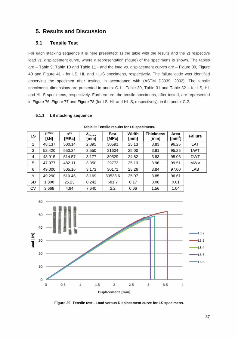
37
5. Results and Discussion
5.1 Tensile Test
For each stacking sequence it is here presented: 1) the table with the results and the 2) respective
load vs. displacement curve, where a representation (figure) of the specimens is shown. The tables
are – Table 9; Table 10 and Table 11 - and the load vs. displacement curves are – Figure 39, Figure
40 and Figure 41 - for LS, HL and HL-S specimens, respectively. The failure code was identified
observing the specimen after testing, in accordance with (ASTM D3039, 2002). The tensile
specimen’s dimensions are presented in annex C.1 - Table 30, Table 31 and Table 32 – for LS, HL
and HL-S specimens, respectively. Furthermore, the tensile specimens, after tested, are represented
in Figure 76, Figure 77 and Figure 78 (for LS, HL and HL-S, respectively), in the annex C.2.
5.1.1 LS stacking sequence
Table 9: Tensile results for LS specimens.
LS [kN]
[MPa]
[mm]
Eest. [MPa]
Width [mm]
Thickness [mm]
Area [mm
2]
Failure
2 48.137 500.14 2.895 30591 25.13 3.83 96.25 LAT
3 52.420 550.34 3.550 31604 25.00 3.81 95.25 LWT
4 48.915 514.57 3.177 30529 24.82 3.83 95.06 DWT
5 47.977 482.11 3.050 29773 25.13 3.96 99.51 MWV
6 49.000 505.16 3.173 30171 25.26 3.84 97.00 LAB
49.290 510.46 3.169 30533.6 25.07 3.85 96.61
SD 1.808 25.23 0.242 681.7 0.17 0.06 0.01
CV 3.668 4.94 7.640 2.2 0.66 1.56 1.04
Figure 39: Tensile test - Load versus Displacement curve for LS specimens.

38
5.1.2 HL stacking sequence
Table 10: Tensile results for HL specimens.
HL [kN]
[MPa]
[mm]
Eest. [MPa]
Width [mm]
Thickness [mm]
Area [mm
2]
Failure
1 38.585 400.13 2.751 29010 25.31 3.81 96.43 AGM
2 36.063 378.14 2.434 29102 25.23 3.78 95.37 AWT
3 37.393 392.03 2.631 28887 25.30 3.77 95.38 LAT
4 37.525 381.81 2.654 28290 25.33 3.88 98.28 AWT
5 37.974 385.40 2.758 27655 25.20 3.91 98.53 AGM
6 35.887 388.02 2.514 30050 25.27 3.66 92.49 AAT
7 38.627 397.91 2.758 28327 25.28 3.84 97.08 AGM
8 38.470 392.60 2.808 27817 25.19 3.89 97.99 AGM
37.565 389.51 2.664 28642.3 25.26 3.82 96.44
SD 1.086 7.62 0.132 780.8 0.05 0.08 0.00
CV 2.892 1.96 4.968 2.7 0.21 2.14 0.44
Figure 40: Tensile test - Load versus Displacement curve for HL specimens.
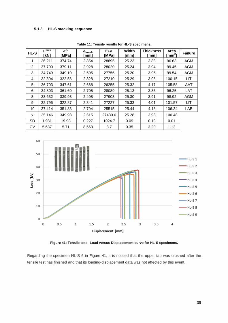
39
5.1.3 HL-S stacking sequence
Table 11: Tensile results for HL-S specimens.
HL-S [kN]
[MPa]
[mm]
Eest. [MPa]
Width [mm]
Thickness [mm]
Area [mm
2]
Failure
1 36.211 374.74 2.854 28895 25.23 3.83 96.63 AGM
2 37.700 379.11 2.928 28020 25.24 3.94 99.45 AGM
3 34.749 349.10 2.505 27756 25.20 3.95 99.54 AGM
4 32.304 322.56 2.328 27210 25.29 3.96 100.15 LIT
5 36.703 347.61 2.668 26255 25.32 4.17 105.58 AAT
6 34.803 361.60 2.705 28089 25.13 3.83 96.25 LAT
8 33.632 339.98 2.408 27908 25.30 3.91 98.92 AGM
9 32.795 322.87 2.341 27227 25.33 4.01 101.57 LIT
10 37.414 351.83 2.794 25515 25.44 4.18 106.34 LAB
35.146 349.93 2.615 27430.6 25.28 3.98 100.48
SD 1.981 19.98 0.227 1024.7 0.09 0.13 0.01
CV 5.637 5.71 8.663 3.7 0.35 3.20 1.12
Figure 41: Tensile test - Load versus Displacement curve for HL-S specimens.
Regarding the specimen HL-S 6 in Figure 41, it is noticed that the upper tab was crushed after the
tensile test has finished and that its loading-displacement data was not affected by this event.

40
5.1.4 Discussion
Due to the mechanical properties of carbon fiber, the tensile test is challenging. The biggest challenge
is to grip the specimen without introducing unacceptable stress concentrations (Adams, 2006). Ideally,
the grips are clamped onto the specimen ends, thus transferring the applied tensile force via shear at
the specimen surfaces, into tensile stresses within the specimen. In composites these clamping forces
are considerable. One approach is to produce specimen as thin as possible. Another approach is to
increase the grip length in order to distribute the force over a larger area. As commercially available
grips are of limited length, it becomes increasingly difficult to grip the specimen uniformly as length
increases. A widespread method to mitigate these problems is to cushion the grip forces by using
pads at the specimen ends. These end tabs may be bonded to the specimen, thus transferring the
shear forces through the adhesive, or simply clamped into position, relying on friction to transfer the
shear loads. The most used method is to bond tabs as they are very effective in cushioning the grip
forces and protecting the specimen surfaces from abrasion. The concern in bonding tabs is the
induction of a new source of stress concentrations, associated with the discontinuity created at the
gage length of the tabs. To avoid this problem, tapering of the tabs is used. The standard ASTM
D3039 recommends a minimum tapering angle of 5°. A 90° taper implies no tapper at all – it is known
as the square tabs. The taper angle can be even greater than 90°, but no benefits have been
demonstrated (Adams, 2006).
During tensile loading, tab ends tend to curl away from the specimen, inducing through-the-thickness
stresses which potentially can peel off the surface layers of the specimen, thus weakening it. Square
tabs resist better to curling than others as they are stiffer and can be gripped right up to their ends,
inhibiting curling. Highly tapered tabs, on the other hand, are very flexible, meaning they do not
necessarily induce high through-the-thickness stresses in the specimen. Another parameter without a
standard consensus is the material of the tab, but ASTM D3039 affirms the most consistently used
bonded tab material has been continuous E-glass fiber-reinforced polymer matrix materials (woven or
un-woven) in a [0/90]ns laminate configuration.
In the tensile tests performed, squares tabs were used, as recommended in some standards,
especially in Europe (European Committee for Standardization, 1995) and Japan (Japanese
Standards Association , 1988).
As cited in (ASTM D3039, 2002), many filamentary composite materials show essentially bilinear
behavior during loading such as seen in plots of either longitudinal stress vs. longitudinal strain or
transverse strain vs. long longitudinal strain. There are different physical reasons for the existence of a
transition region, such as matrix cracking under tensile loading or ply delamination.
Table 12: Tensile test results.
Laminate [MPa] Eest [GPa]
LS 510.46 30.53
HL 389.51 28.64
HL-S 349.93 27.43
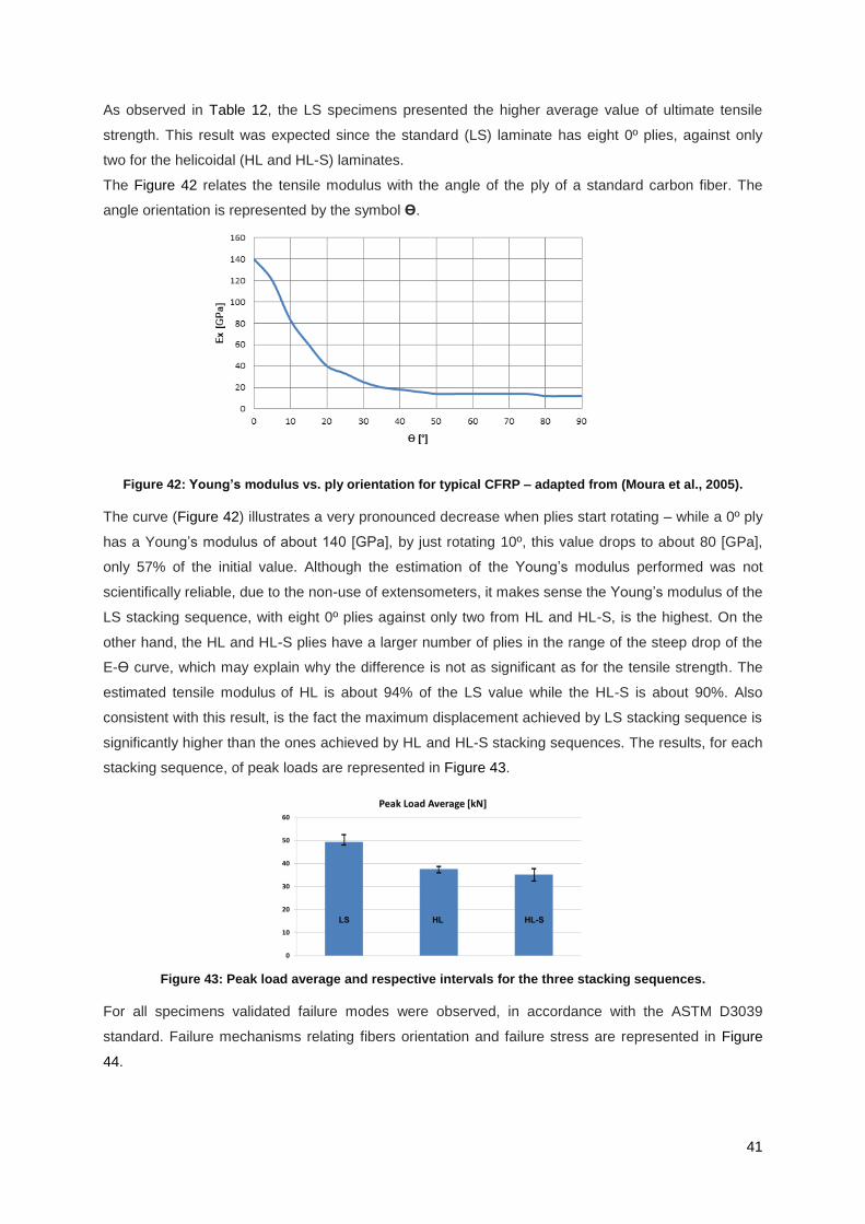
41
As observed in Table 12, the LS specimens presented the higher average value of ultimate tensile
strength. This result was expected since the standard (LS) laminate has eight 0º plies, against only
two for the helicoidal (HL and HL-S) laminates.
The Figure 42 relates the tensile modulus with the angle of the ply of a standard carbon fiber. The
angle orientation is represented by the symbol ϴ.
Figure 42: Young’s modulus vs. ply orientation for typical CFRP – adapted from (Moura et al., 2005).
The curve (Figure 42) illustrates a very pronounced decrease when plies start rotating – while a 0º ply
has a Young’s modulus of about 140 [GPa], by just rotating 10º, this value drops to about 80 [GPa],
only 57% of the initial value. Although the estimation of the Young’s modulus performed was not
scientifically reliable, due to the non-use of extensometers, it makes sense the Young’s modulus of the
LS stacking sequence, with eight 0º plies against only two from HL and HL-S, is the highest. On the
other hand, the HL and HL-S plies have a larger number of plies in the range of the steep drop of the
E-ϴ curve, which may explain why the difference is not as significant as for the tensile strength. The
estimated tensile modulus of HL is about 94% of the LS value while the HL-S is about 90%. Also
consistent with this result, is the fact the maximum displacement achieved by LS stacking sequence is
significantly higher than the ones achieved by HL and HL-S stacking sequences. The results, for each
stacking sequence, of peak loads are represented in Figure 43.
Figure 43: Peak load average and respective intervals for the three stacking sequences.
For all specimens validated failure modes were observed, in accordance with the ASTM D3039
standard. Failure mechanisms relating fibers orientation and failure stress are represented in Figure
44.
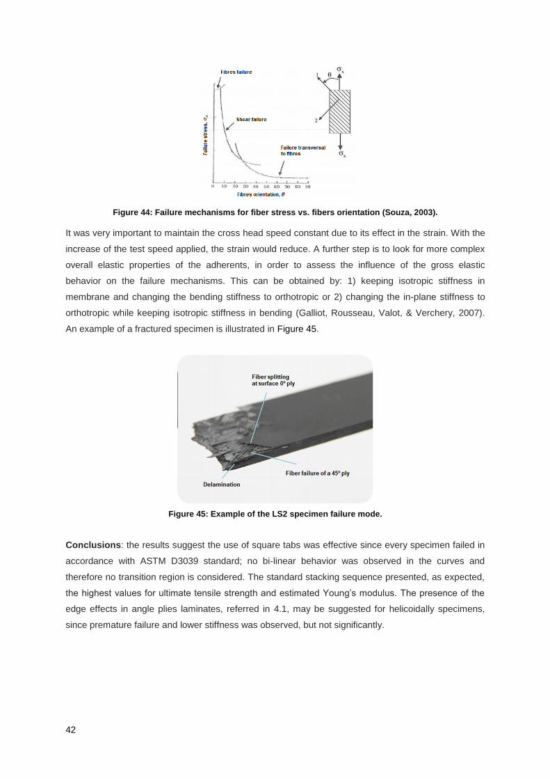
42
Figure 44: Failure mechanisms for fiber stress vs. fibers orientation (Souza, 2003).
It was very important to maintain the cross head speed constant due to its effect in the strain. With the
increase of the test speed applied, the strain would reduce. A further step is to look for more complex
overall elastic properties of the adherents, in order to assess the influence of the gross elastic
behavior on the failure mechanisms. This can be obtained by: 1) keeping isotropic stiffness in
membrane and changing the bending stiffness to orthotropic or 2) changing the in-plane stiffness to
orthotropic while keeping isotropic stiffness in bending (Galliot, Rousseau, Valot, & Verchery, 2007).
An example of a fractured specimen is illustrated in Figure 45.
Figure 45: Example of the LS2 specimen failure mode.
Conclusions: the results suggest the use of square tabs was effective since every specimen failed in
accordance with ASTM D3039 standard; no bi-linear behavior was observed in the curves and
therefore no transition region is considered. The standard stacking sequence presented, as expected,
the highest values for ultimate tensile strength and estimated Young’s modulus. The presence of the
edge effects in angle plies laminates, referred in 4.1, may be suggested for helicoidally specimens,
since premature failure and lower stiffness was observed, but not significantly.

43
5.2 Interlaminar Shear Strength Test [ILSS]
For each stacking sequence, the tables with the final results – Table 13, Table 14 and Table 15 for LS,
HL and HL-S specimens, respectively – and the load vs. displacement curves, with the figures of the
respective specimens tested are presented - Figure 46, Figure 47 and Figure 48 for LS, HL and HL-S
specimens, respectively. The pictures for all specimens are shown in annex D. As explained in 4.2,
the nominal dimensions of the specimens were 12 [mm] of width and 40 [mm] of length.
5.2.1 LS stacking sequence
Table 13: Interlaminar shear strength results for LS specimens.
Specimen Pm [N] Fsbs [MPa] h [mm] b [mm] Span [mm] S/h Failure Mode
LS 1 1669.955 28.13 3.71 12.00 18.55 5.00 Interlam. Shear + Flexure
LS 2 1557.676 26.48 3.86 11.43 19.30 5.00 Interlam. Shear + Flexure
LS 4 1617.662 26.22 3.83 12.08 19.15 5.00 Interlam. Shear + Flexure
LS 7 1486.659 23.90 3.85 12.12 19.23 4.99 Interlam. Shear + Flexure
LS 10 1729.512 27.70 3.88 12.07 19.38 4.99 Interlam. Shear + Flexure
LS 11 1557.573 25.05 3.86 12.08 19.28 4.99 Interlam. Shear + Flexure
1603.173 26.25 3.83 11.96 19.15 5.00
SD 87.586 1.59 0.06 0.26 0.30 4.90
CV 5.463 6.07 1.61 2.21 1.58 0.98
Figure 46: Load versus displacement curves for LS specimens.
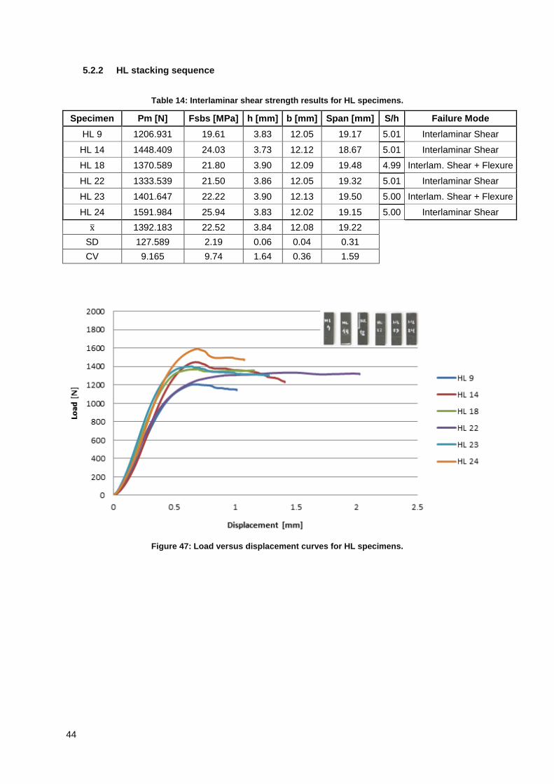
44
5.2.2 HL stacking sequence
Table 14: Interlaminar shear strength results for HL specimens.
Specimen Pm [N] Fsbs [MPa] h [mm] b [mm] Span [mm] S/h Failure Mode
HL 9 1206.931 19.61 3.83 12.05 19.17 5.01 Interlaminar Shear
HL 14 1448.409 24.03 3.73 12.12 18.67 5.01 Interlaminar Shear
HL 18 1370.589 21.80 3.90 12.09 19.48 4.99 Interlam. Shear + Flexure
HL 22 1333.539 21.50 3.86 12.05 19.32 5.01 Interlaminar Shear
HL 23 1401.647 22.22 3.90 12.13 19.50 5.00 Interlam. Shear + Flexure
HL 24 1591.984 25.94 3.83 12.02 19.15 5.00 Interlaminar Shear
1392.183 22.52 3.84 12.08 19.22
SD 127.589 2.19 0.06 0.04 0.31
CV 9.165 9.74 1.64 0.36 1.59
Figure 47: Load versus displacement curves for HL specimens.
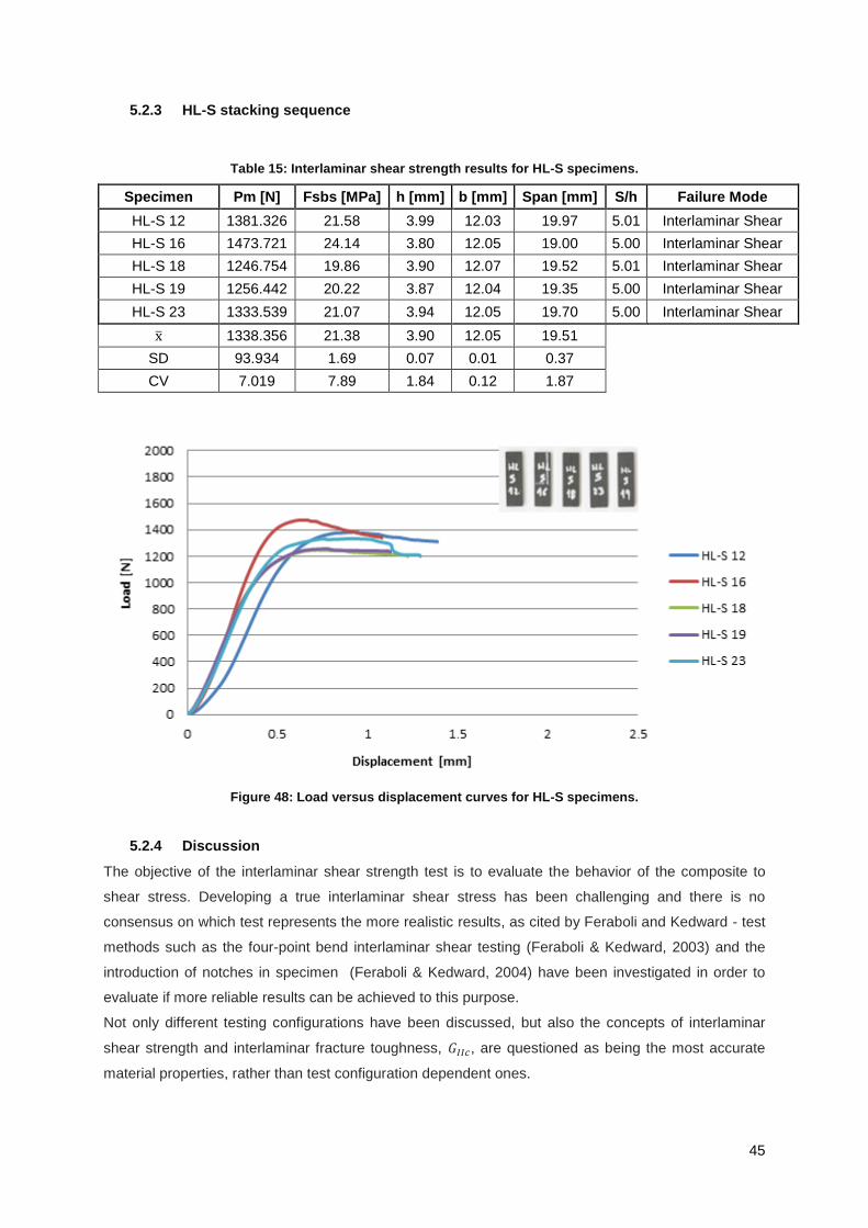
45
5.2.3 HL-S stacking sequence
Table 15: Interlaminar shear strength results for HL-S specimens.
Specimen Pm [N] Fsbs [MPa] h [mm] b [mm] Span [mm] S/h Failure Mode
HL-S 12 1381.326 21.58 3.99 12.03 19.97 5.01 Interlaminar Shear
HL-S 16 1473.721 24.14 3.80 12.05 19.00 5.00 Interlaminar Shear
HL-S 18 1246.754 19.86 3.90 12.07 19.52 5.01 Interlaminar Shear
HL-S 19 1256.442 20.22 3.87 12.04 19.35 5.00 Interlaminar Shear
HL-S 23 1333.539 21.07 3.94 12.05 19.70 5.00 Interlaminar Shear
1338.356 21.38 3.90 12.05 19.51
SD 93.934 1.69 0.07 0.01 0.37
CV 7.019 7.89 1.84 0.12 1.87
Figure 48: Load versus displacement curves for HL-S specimens.
5.2.4 Discussion
The objective of the interlaminar shear strength test is to evaluate the behavior of the composite to
shear stress. Developing a true interlaminar shear stress has been challenging and there is no
consensus on which test represents the more realistic results, as cited by Feraboli and Kedward - test
methods such as the four-point bend interlaminar shear testing (Feraboli & Kedward, 2003) and the
introduction of notches in specimen (Feraboli & Kedward, 2004) have been investigated in order to
evaluate if more reliable results can be achieved to this purpose.
Not only different testing configurations have been discussed, but also the concepts of interlaminar
shear strength and interlaminar fracture toughness, , are questioned as being the most accurate
material properties, rather than test configuration dependent ones.
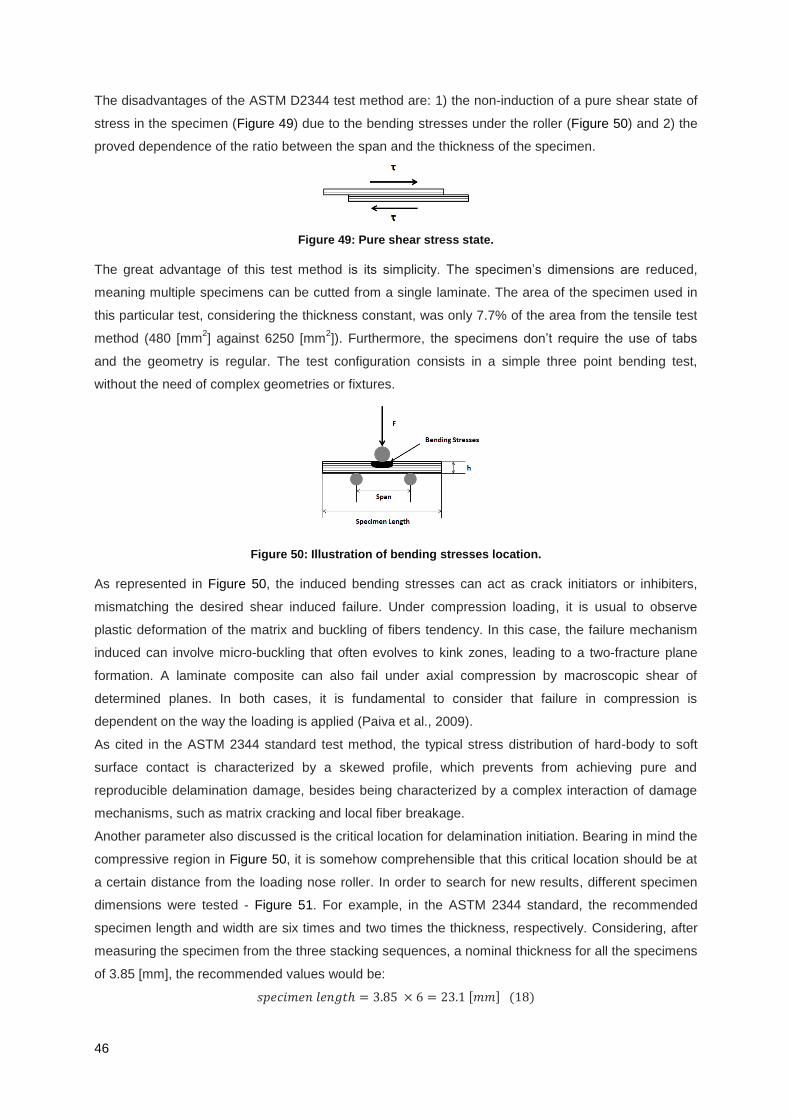
46
The disadvantages of the ASTM D2344 test method are: 1) the non-induction of a pure shear state of
stress in the specimen (Figure 49) due to the bending stresses under the roller (Figure 50) and 2) the
proved dependence of the ratio between the span and the thickness of the specimen.
Figure 49: Pure shear stress state.
The great advantage of this test method is its simplicity. The specimen’s dimensions are reduced,
meaning multiple specimens can be cutted from a single laminate. The area of the specimen used in
this particular test, considering the thickness constant, was only 7.7% of the area from the tensile test
method (480 [mm2] against 6250 [mm
2]). Furthermore, the specimens don’t require the use of tabs
and the geometry is regular. The test configuration consists in a simple three point bending test,
without the need of complex geometries or fixtures.
Figure 50: Illustration of bending stresses location.
As represented in Figure 50, the induced bending stresses can act as crack initiators or inhibiters,
mismatching the desired shear induced failure. Under compression loading, it is usual to observe
plastic deformation of the matrix and buckling of fibers tendency. In this case, the failure mechanism
induced can involve micro-buckling that often evolves to kink zones, leading to a two-fracture plane
formation. A laminate composite can also fail under axial compression by macroscopic shear of
determined planes. In both cases, it is fundamental to consider that failure in compression is
dependent on the way the loading is applied (Paiva et al., 2009).
As cited in the ASTM 2344 standard test method, the typical stress distribution of hard-body to soft
surface contact is characterized by a skewed profile, which prevents from achieving pure and
reproducible delamination damage, besides being characterized by a complex interaction of damage
mechanisms, such as matrix cracking and local fiber breakage.
Another parameter also discussed is the critical location for delamination initiation. Bearing in mind the
compressive region in Figure 50, it is somehow comprehensible that this critical location should be at
a certain distance from the loading nose roller. In order to search for new results, different specimen
dimensions were tested - Figure 51. For example, in the ASTM 2344 standard, the recommended
specimen length and width are six times and two times the thickness, respectively. Considering, after
measuring the specimen from the three stacking sequences, a nominal thickness for all the specimens
of 3.85 [mm], the recommended values would be:
( )

47
( )
The width used was 55.8% greater than the recommended and the length about 73.1% greater.
Figure 51: Used geometry versus recommended geometry by ASTM D2344.
For this test method, the typical damage initiation is characterized by a single crack that propagates
from a region located about one thickness away from the roller, usually at the axis of symmetry or
within a one fourth of the thickness above. A sharp drop in the load-displacement curve and an
audible cracking sound accompany catastrophic delamination. After the first inter-ply failure, the load
picks up again and in some cases it may reach the pristine value - where is nearly constant. The
delamination is often located near the vertical axis of symmetry and right at the mid-plane, actually
one ply above it - Figure 52 (Feraboli & Kedward, 2004).
Figure 52: Illustration of the typical crack initiation and delamination.
The highest fiber orientation angle mismatch appears to favor the path of self-consistent cracks such
as delaminations. The interlaminar shear stress distribution through the thickness obtained from beam
theory is accurate in the range of one to two thicknesses away from the rollers, where the influence of
contact forces on the stress profile diminishes. Feraboli and Kedward demonstrated that a more
uniform shear stress state can be achieved for specimens with higher span to thickness ratios and its
peak value is closer to the maximum value predicted by the beam theory (Feraboli & Kedward, 2004).
Furthermore, the peak value achieved experimentally is sustained over a greater length, therefore
allowing for a greater strain energy density to accumulate.
Delamination is generally visible to the naked eye in this test, but sometimes it is necessary to magnify
the image. This can be done with a magnifying glass or, if necessary, with a microscope. When
evaluating the failure mode, it was observed for eight specimens – including all with the LS stacking
sequence, the flexural behavior - represented in Figure 36. For the specimen LS4 - Figure 53, it is
visible the cracking due to tension in the bottom surface.
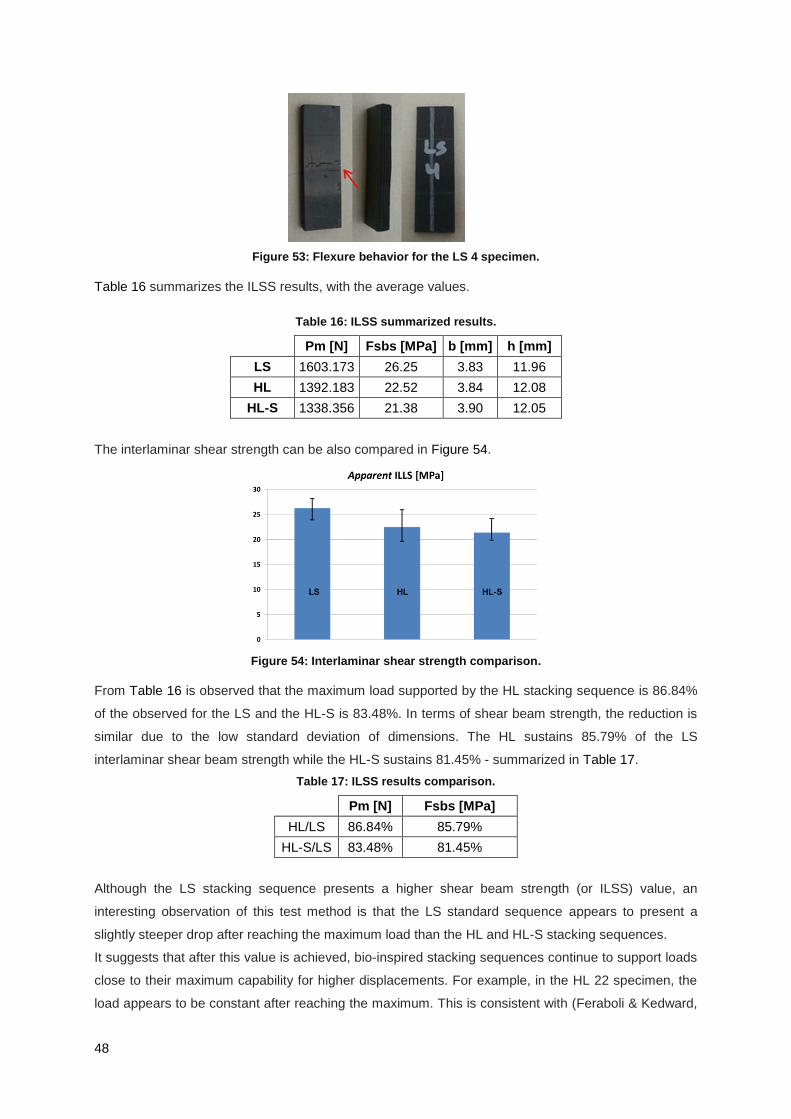
48
Figure 53: Flexure behavior for the LS 4 specimen.
Table 16 summarizes the ILSS results, with the average values.
Table 16: ILSS summarized results.
Pm [N] Fsbs [MPa] b [mm] h [mm]
LS 1603.173 26.25 3.83 11.96
HL 1392.183 22.52 3.84 12.08
HL-S 1338.356 21.38 3.90 12.05
The interlaminar shear strength can be also compared in Figure 54.
Figure 54: Interlaminar shear strength comparison.
From Table 16 is observed that the maximum load supported by the HL stacking sequence is 86.84%
of the observed for the LS and the HL-S is 83.48%. In terms of shear beam strength, the reduction is
similar due to the low standard deviation of dimensions. The HL sustains 85.79% of the LS
interlaminar shear beam strength while the HL-S sustains 81.45% - summarized in Table 17.
Table 17: ILSS results comparison.
Pm [N] Fsbs [MPa]
HL/LS 86.84% 85.79%
HL-S/LS 83.48% 81.45%
Although the LS stacking sequence presents a higher shear beam strength (or ILSS) value, an
interesting observation of this test method is that the LS standard sequence appears to present a
slightly steeper drop after reaching the maximum load than the HL and HL-S stacking sequences.
It suggests that after this value is achieved, bio-inspired stacking sequences continue to support loads
close to their maximum capability for higher displacements. For example, in the HL 22 specimen, the
load appears to be constant after reaching the maximum. This is consistent with (Feraboli & Kedward,

49
2003), where is cited that the composite can continue to sustain considerable loads way beyond
fracture initiation, particularly for laminates with multiple fiber orientation. In their work they tested
three stacking sequences of impregnated carbon fiber - unidirectional, a cross-ply and quasi-isotropic
to obtain values of ILSS and flexural strengths. The results are described in Table 18.
Table 18: ILSS and Flexural Results - (Feraboli & Kedward, 2003).
ILSS [MPa] Flexural strength [MPa]
[0]s 76.6 1235
[0/90]s 76.9 853
[0/ 45/90]s 76.5 894
Average 76.7 994
SD 0.2 210
CV 0.3 21
As demonstrated in Table 18, while changing fiber orientations had low influence on the shear beam
strength, a strong influence on flexural strength values was noted. Interlaminar shear stress develops
at the free edge of multidirectional laminates and at local discontinuities such as ply-drops, notches,
bonded or bolted joints, where ply stresses must become zero to satisfy boundary conditions (Feraboli
& Kedward, 2003). But (Pagano & Pipes, 1971) found, theoretically, that keeping the angle, symmetry
and number of plies, but changing the stacking sequence influences interlaminar stresses. The key
when changing the stacking sequence is to decrease the interlaminar shear stresses, without
increasing the tensile (if any) interlaminar normal stresses. For example, a laminate with the stacking
sequence [+-30/90]s produces tensile interlaminar normal stresses under a uniaxial tensile load, while
the stacking sequence [90/+-30]s it produces compressive interlaminar normal stresses. This makes
the latter sequence less prone to delamination. Alternative techniques to improve tolerance to
delamination include using toughened resin systems and interleaved systems, where a discrete layer
of resin with high toughness and strain to failure is added on top of the layer.
A similar result to this test was achieved by (Turla, Kumar, Reddy, & Shekar, 2014) where they
obtained an average result of 30.11 [MPa] for the filament winding processed carbon fiber of five
specimens, composed by a quasi-isotropic stacking sequence, with the nominal dimensions 8 x 3.8 x
50 [mm]. The span to thickness ratio was 6, with the same thickness, 33% narrower and 25% longer
specimens.
Conclusion: since flexure was observed for the all standard LS specimens, it is suggested that the
interlaminar shear strength determined for this stacking sequence does not truly represents
interlaminar failure, but the helicoidal stacking sequences (HL and HL-S) suggest a more reliable
interlaminar shear strength results.
50
5.3 Impact Test
The impact response understanding is critical for the project of structural composite materials.
In this subchapter the curves derived from the equations (15), (16) and (17) - in 4.3, are presented and
discussed for each impact energy level.
In order to understand the correlations performed, an explanation for each one is drawn:
Force vs. Time: during a weight-drop impact, the force–time curve is set to start when the recorded
contact force becomes positive, leading to an initial positive slope. The curve reaches a maximum
force and drops until the force becomes zero. During the force increase it may be observed a
significant load drop (discontinuity or slope) if the load reaches a threshold value, known as F1 (ASTM
D7136, 2015).
The force vs. time curve may also include significant oscillations with relatively close peak forces and
intervals, which difficult the characterization of the delamination initiation and damage mechanisms
(Farooq & Myler, 2015). The authors just cited correlate the maximum damage size of the laminate
with F1. However, as cited by (González et al., 2011), C-Scan (ultrasonic) inspections provide the
projected delamination area at the end of the impact test, meaning these results do not reveal clearly
whether the critical force F1 corresponds to the generation of a single delamination or a set of
delaminations.
For low energy values, where the corresponding threshold value is not reached, the force-time curve
presents a bell-shaped profile (González, Maimí, Sainz de Aja, Cruz, & Camanho, 2014). It is also
worth noting that, in the mechanical response of the laminate (observed in both the force vs. time and
force vs. displacement curves) a clear drop does not have to occur, rather it can appear with a point
from which small oscillations start. The referred point also indicates that the elastic loading stage is
over and that damage is developing in the material in a slowest and progressively way, due to a
different sequence of the failure mechanisms. Depending on the impact velocity, F1 can be equal to
Fmax. After reaching force F1, the damage process initiates with localized matrix cracks and fiber-matrix
interfacial debonding, generally not detectable by NDT methods (González et al., 2011). It is important
to refer that F1 does not physically represents the initiation of damage, as sub-critical matrix cracks
and small delaminations may initiate at lower forces. It simply represents the initial value where a
significant change in stiffness is detected. The identification of F1 is sometimes challenging due to the
effects of the governing parameters, harmonic resonances - of the load cell or of the specimen during
impact (González et al., 2011). In the last cited work, the authors concluded that F1 is independent of
the impact velocity, since they used the same impactor for three different energy levels of impact
(19.3, 28.6 and 38.6J). The authors also observed that the peak loads Fmax and the slopes of the
elastic regime increased by increasing the velocity, for different laminates (González et al., 2011). In a
summarized way, the referred authors concluded that:
- by increasing the velocity, the response is extended in time because the specimen develops
more damage. The impact time (or contact duration) increases due to reduced bending
stiffness of the structure;
- constant threshold force for different impact velocities;
- ply clustering resulted in lower threshold and peak forces, under the same impact conditions;
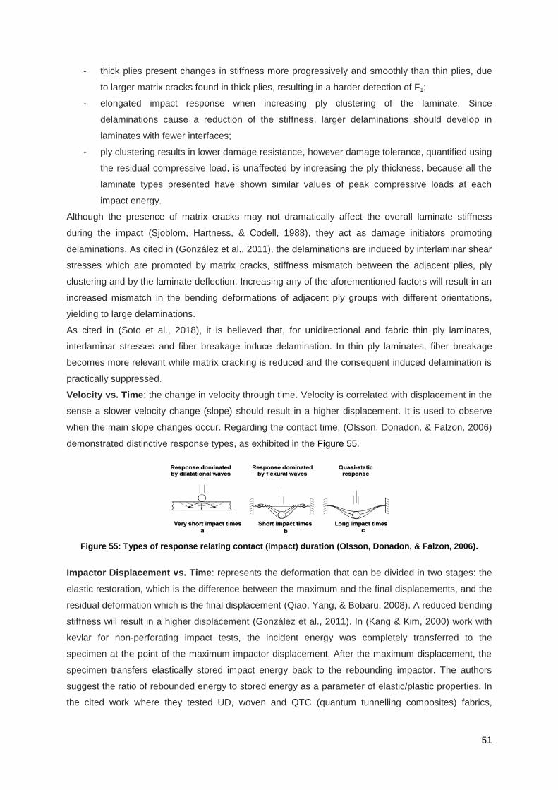
51
- thick plies present changes in stiffness more progressively and smoothly than thin plies, due
to larger matrix cracks found in thick plies, resulting in a harder detection of F1;
- elongated impact response when increasing ply clustering of the laminate. Since
delaminations cause a reduction of the stiffness, larger delaminations should develop in
laminates with fewer interfaces;
- ply clustering results in lower damage resistance, however damage tolerance, quantified using
the residual compressive load, is unaffected by increasing the ply thickness, because all the
laminate types presented have shown similar values of peak compressive loads at each
impact energy.
Although the presence of matrix cracks may not dramatically affect the overall laminate stiffness
during the impact (Sjoblom, Hartness, & Codell, 1988), they act as damage initiators promoting
delaminations. As cited in (González et al., 2011), the delaminations are induced by interlaminar shear
stresses which are promoted by matrix cracks, stiffness mismatch between the adjacent plies, ply
clustering and by the laminate deflection. Increasing any of the aforementioned factors will result in an
increased mismatch in the bending deformations of adjacent ply groups with different orientations,
yielding to large delaminations.
As cited in (Soto et al., 2018), it is believed that, for unidirectional and fabric thin ply laminates,
interlaminar stresses and fiber breakage induce delamination. In thin ply laminates, fiber breakage
becomes more relevant while matrix cracking is reduced and the consequent induced delamination is
practically suppressed.
Velocity vs. Time: the change in velocity through time. Velocity is correlated with displacement in the
sense a slower velocity change (slope) should result in a higher displacement. It is used to observe
when the main slope changes occur. Regarding the contact time, (Olsson, Donadon, & Falzon, 2006)
demonstrated distinctive response types, as exhibited in the Figure 55.
Figure 55: Types of response relating contact (impact) duration (Olsson, Donadon, & Falzon, 2006).
Impactor Displacement vs. Time: represents the deformation that can be divided in two stages: the
elastic restoration, which is the difference between the maximum and the final displacements, and the
residual deformation which is the final displacement (Qiao, Yang, & Bobaru, 2008). A reduced bending
stiffness will result in a higher displacement (González et al., 2011). In (Kang & Kim, 2000) work with
kevlar for non-perforating impact tests, the incident energy was completely transferred to the
specimen at the point of the maximum impactor displacement. After the maximum displacement, the
specimen transfers elastically stored impact energy back to the rebounding impactor. The authors
suggest the ratio of rebounded energy to stored energy as a parameter of elastic/plastic properties. In
the cited work where they tested UD, woven and QTC (quantum tunnelling composites) fabrics,

52
unidirectional laminate showed improved elastic characteristics, such as higher rebounding energy,
lower displacement and shorter total impact time.
Energy Absorbed vs. Time: used to correlate and predict strain and elastic energy levels during an
impact event. The authors (Kang & Kim, 2000) suggested an approach to interpret the energy-time
history for kevlar composites. Assuming no fiber breakage occurs under low level of impact energy,
the curve is interpreted in two major parts: an elastically stored energy by the specimen and
transferred back to the impactor, and an absorbed energy by the specimen - part dissipated in its
damage initiation and propagation, and other part absorbed by the impact system in vibration, heat
and inelastic behavior of the impactor or supports. The total energy absorbed by the specimen has
three components: Emb, Ebd and Edel, which represent, respectively, membrane energy, bending
energy and energy absorbed by the initiation of damages in the matrix. In the work cited no attempts
were made to distinguish delamination and matrix cracking, since matrix cracking is associated with
delamination and the ratio between the matrix cracking area and the delamination area is constant for
a given system, or the energy absorption by matrix cracking is often negligible. If the fracture
toughness of the laminate is known, the energy needed to delaminate a given area can be estimated.
In order obtain a precise estimation of the delaminated area, a destructive technique is necessary: the
de-ply technique. (Kang & Kim, 2000) considered that the energy absorption mechanisms available in
composite materials were: 1) fiber breakage; 2) membrane deformation; 3) bending deformation and
4) delamination. For low velocity impacts, the last two were the major energy absorption mechanisms.
At energies above the threshold, the fracture area presents a conical shape with the overall area of
damage increasing towards the lower surface of the composite. For high velocity impacts, at the
perforation threshold energy, the spherical tipped impactor usually creates a conically shaped shear
plug as it penetrates the specimen and energy is dissipated during the process. Thus, for high velocity
impacts, the energy absorption mechanisms could be classified as: 1) global deformation; 2) fiber
breakage; 3) delamination and 4) shear-out.
The last energy recorded in the curve represents the energy dissipated by the specimen during the
impact event and is also known as the absorbed energy.
The impact can be also divided in two stages: 1) initial phase where the impact energy imparted by the
impactor is absorbed by elastic-plastic deformation, as well as inter/intra-laminar damage within the
laminate; and 2) the rebound phase where the elastic deformation of the laminate is recovered. The
elastic energy is the only part recovered by the laminate during the rebound phase. This leads to a
lower slope in the second phase.
Force vs. Displacement: this curve exhibits the laminate’s stiffness (slope of the curve), the
maximum displacement and absorbed energy. (Farooq & Myler, 2015) also suggested dividing the
load-deflection in four parts. The first part of the curve is linear and represents the stiffness of the non-
damaged laminate. The second part of the force-displacement curve shows a load drop as a clear
change in stiffness, indicating damage initiation. Third and fourth parts are concerned with through-
thickness parameters and perforation. The area under the curve corresponds to the dissipated energy.
It is noted that, since the energy levels are different, the scales in the curves presented are also
different, in order to maximize the visual aspect.
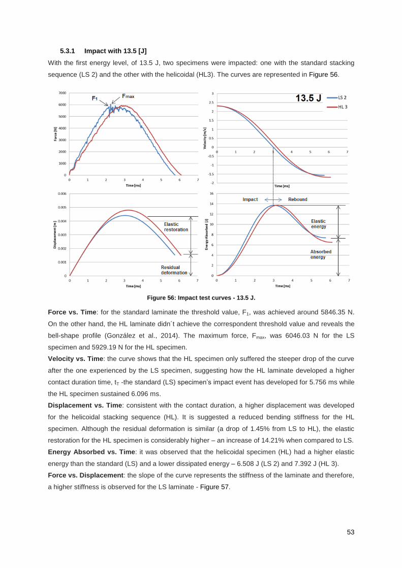
53
5.3.1 Impact with 13.5 [J]
With the first energy level, of 13.5 J, two specimens were impacted: one with the standard stacking
sequence (LS 2) and the other with the helicoidal (HL3). The curves are represented in Figure 56.
Figure 56: Impact test curves - 13.5 J.
Force vs. Time: for the standard laminate the threshold value, F1, was achieved around 5846.35 N.
On the other hand, the HL laminate didn´t achieve the correspondent threshold value and reveals the
bell-shape profile (González et al., 2014). The maximum force, Fmax, was 6046.03 N for the LS
specimen and 5929.19 N for the HL specimen.
Velocity vs. Time: the curve shows that the HL specimen only suffered the steeper drop of the curve
after the one experienced by the LS specimen, suggesting how the HL laminate developed a higher
contact duration time, tT -the standard (LS) specimen’s impact event has developed for 5.756 ms while
the HL specimen sustained 6.096 ms.
Displacement vs. Time: consistent with the contact duration, a higher displacement was developed
for the helicoidal stacking sequence (HL). It is suggested a reduced bending stiffness for the HL
specimen. Although the residual deformation is similar (a drop of 1.45% from LS to HL), the elastic
restoration for the HL specimen is considerably higher – an increase of 14.21% when compared to LS.
Energy Absorbed vs. Time: it was observed that the helicoidal specimen (HL) had a higher elastic
energy than the standard (LS) and a lower dissipated energy – 6.508 J (LS 2) and 7.392 J (HL 3).
Force vs. Displacement: the slope of the curve represents the stiffness of the laminate and therefore,
a higher stiffness is observed for the LS laminate - Figure 57.

54
Figure 57: Force vs. Displacement – Impact with 13.5 J.
5.3.2 Impact with 25 [J]
For this impact energy level, one standard stacking sequence (LS 1), one helicoidal (HL 2) and two
helicoidal-symmetric HL-S specimens were tested (HL-S 1 and HL-S 2). The test curves are illustrated
in Figure 58.
Figure 58: Impact test curves - 25 J.
Force vs. Time: for this impact energy only the HL-S 2 didn’t reach its threshold value, F1, and
therefore exhibits the bell-shape profile. An important difference during the production process of the
helicoidal laminates (HL) was that in HL-S 2 production, a peel-ply was placed in the glass surface.
For the other specimens, the threshold values were: 6639.73 N (at 1.520 ms) for LS 1, for HL 2 there
isn’t a significant load drop before the maximum force, and a less significant threshold of 8378 N
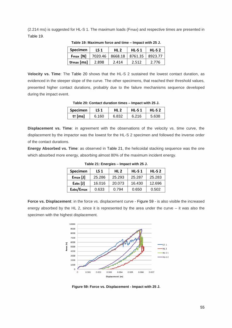
55
(2.214 ms) is suggested for HL-S 1. The maximum loads (Fmax) and respective times are presented in
Table 19.
Table 19: Maximum force and time – Impact with 25 J.
Specimen LS 1 HL 2 HL-S 1 HL-S 2
Fmax [N] 7020.46 8668.18 8761.35 8923.77
tFmax [ms] 2.898 2.414 2.512 2.776
Velocity vs. Time: The Table 20 shows that the HL-S 2 sustained the lowest contact duration, as
evidenced in the steeper slope of the curve. The other specimens, that reached their threshold values,
presented higher contact durations, probably due to the failure mechanisms sequence developed
during the impact event.
Table 20: Contact duration times – Impact with 25 J.
Specimen LS 1 HL 2 HL-S 1 HL-S 2
tT [ms] 6.160 6.832 6.216 5.638
Displacement vs. Time: in agreement with the observations of the velocity vs. time curve, the
displacement by the impactor was the lowest for the HL-S 2 specimen and followed the inverse order
of the contact durations.
Energy Absorbed vs. Time: as observed in Table 21, the helicoidal stacking sequence was the one
which absorbed more energy, absorbing almost 80% of the maximum incident energy.
Table 21: Energies – Impact with 25 J.
Specimen LS 1 HL 2 HL-S 1 HL-S 2
Emax [J] 25.286 25.293 25.287 25.283
Eabs [J] 16.016 20.073 16.430 12.696
Eabs/Emax 0.633 0.794 0.650 0.502
Force vs. Displacement: in the force vs. displacement curve - Figure 59 - is also visible the increased
energy absorbed by the HL 2, since it is represented by the area under the curve – it was also the
specimen with the highest displacement.
Figure 59: Force vs. Displacement - Impact with 25 J.
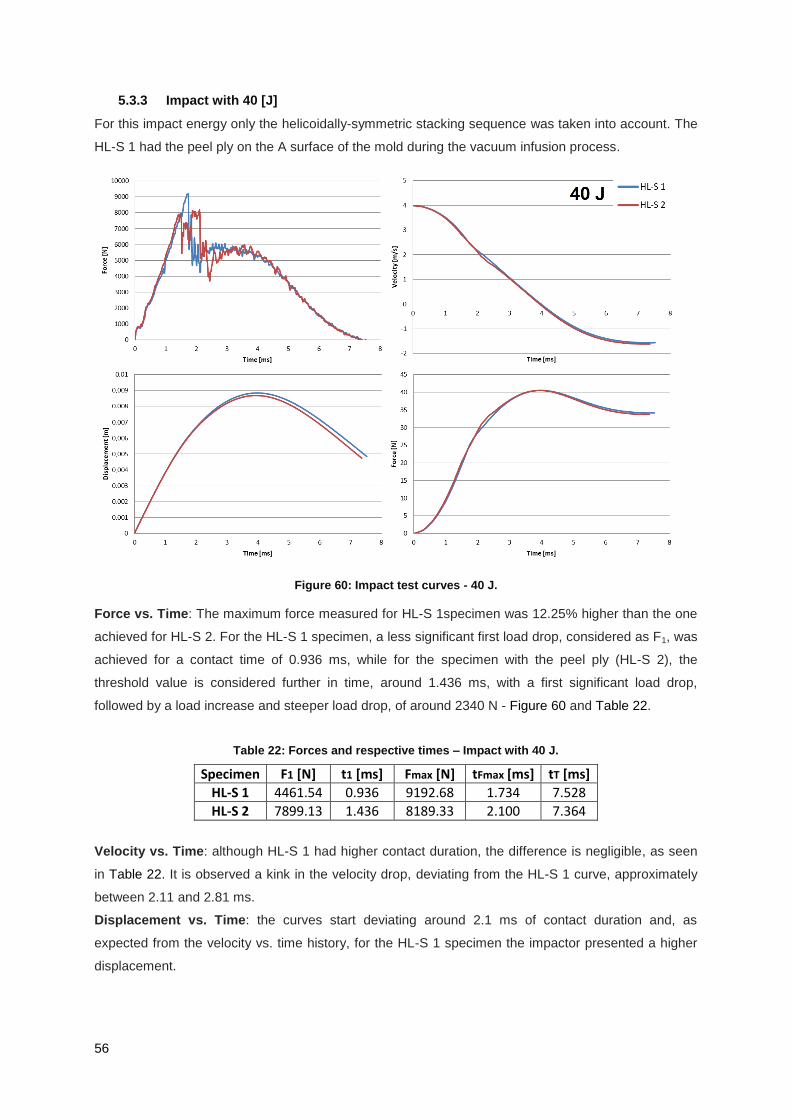
56
5.3.3 Impact with 40 [J]
For this impact energy only the helicoidally-symmetric stacking sequence was taken into account. The
HL-S 1 had the peel ply on the A surface of the mold during the vacuum infusion process.
Figure 60: Impact test curves - 40 J.
Force vs. Time: The maximum force measured for HL-S 1specimen was 12.25% higher than the one
achieved for HL-S 2. For the HL-S 1 specimen, a less significant first load drop, considered as F1, was
achieved for a contact time of 0.936 ms, while for the specimen with the peel ply (HL-S 2), the
threshold value is considered further in time, around 1.436 ms, with a first significant load drop,
followed by a load increase and steeper load drop, of around 2340 N - Figure 60 and Table 22.
Table 22: Forces and respective times – Impact with 40 J.
Specimen F1 [N] t1 [ms] Fmax [N] tFmax [ms] tT [ms]
HL-S 1 4461.54 0.936 9192.68 1.734 7.528
HL-S 2 7899.13 1.436 8189.33 2.100 7.364
Velocity vs. Time: although HL-S 1 had higher contact duration, the difference is negligible, as seen
in Table 22. It is observed a kink in the velocity drop, deviating from the HL-S 1 curve, approximately
between 2.11 and 2.81 ms.
Displacement vs. Time: the curves start deviating around 2.1 ms of contact duration and, as
expected from the velocity vs. time history, for the HL-S 1 specimen the impactor presented a higher
displacement.
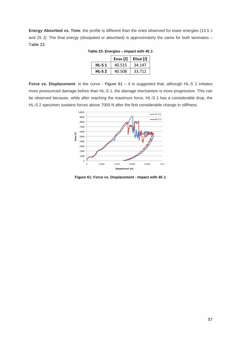
57
Energy Absorbed vs. Time: the profile is different than the ones observed for lower energies (13.5 J
and 25 J). The final energy (dissipated or absorbed) is approximately the same for both laminates –
Table 23.
Table 23: Energies – Impact with 40 J.
Emax [J] Efinal [J]
HL-S 1 40.515 34.147
HL-S 2 40.508 33.712
Force vs. Displacement: in the curve - Figure 61 – it is suggested that, although HL-S 2 initiates
more pronounced damage before than HL-S 1, the damage mechanism is more progressive. This can
be observed because, while after reaching the maximum force, HL-S 1 has a considerable drop, the
HL-S 2 specimen sustains forces above 7000 N after the first considerable change in stiffness.
Figure 61: Force vs. Displacement - Impact with 40 J.

58
5.3.4 Impact with 80 [J]
For this energy level, one helicoidal (HL 1) and two helicoidal-symmetric specimens were tested, with
the impact test curves presented in Figure 62.
Figure 62: Impact test curves – 80 J.
Force vs. Time: in the attempt to determine a first threshold force, three values were taken from the
first significant difference in the curve slope. This value was higher for HL-S laminates than for the HL
one, although HL took more time to reach this lower value. The helicoidal-symmetric specimens also
sustained higher forces than the standard laminate.
Table 24: Impact parameters results – impact with 80 J.
Specimen F1 [N] t1 [ms] Fmax [N] tFmax [ms] tT [ms] Final disp [m] Eabs [J]
HL 1 580.41 0.080 8096.46 1.874 10.980 0.02437 61.765
HL-S 1 612.05 0.078 8309.14 1.800 13.536 0.02385 71.067
HL-S 2 596.05 0.072 9145.11 1.906 14.356 0.02328 74.700
Velocity vs. Time: from this curve it is concluded that the deepest the slope become, the higher the
contact duration was. The contact duration of the HL-S specimens were 23.3% and 30.7%,
respectively for HL-S 1 and HL-S 2, higher than the one experienced by HL specimen.
Displacement vs. Time: the final displacements are displayed in Table 24.
Energy Absorbed vs. Time: since perforation of the specimen occurred, there was no elastic energy
restoration. The final energies were the maximum absorbed by the specimens. It is concluded that, in
this test, higher energy absorption was achieved for HL-S specimens. From the curve observable in

59
Figure 62 it is believed, although more data is necessary to prove it, the energy absorption of the HL-S
stacking sequences is definitely larger than for the HL laminates.
In high-velocity impact conditions, the contact time between the impactor and the target is very short.
In the impact with the higher energy (80 J), is seen the contact time is greater than for the other
impacts. Thus it is readily understood, without analyzing the impactor velocity, this is not a case of
high impact velocity. In high velocity impacts the total energy absorbing capability of the specimen is
not utilized and the impactor induces a much localized form of target response.
Force vs. Displacement: the force vs. displacement curve is presented in Figure 63.
Figure 63: Force vs. Displacement - Impact with 80 J.
5.3.5 Discussion
As in (González et al., 2011), by increasing the impact velocity, the response was elongated in time.
For the three impact energy levels of 13.5 J, 25 J and 40 J, the mass is the same and the impact
velocity increases from 2.314 to 3.147 and finally 3.986 (m/s), respectively, while the respective
average contact durations for each energy level are: 5.926, 6.212 and 7.446 ms. For the impacts with
80 J, the average contact duration was 12.957 ms, with a lower velocity than the 40 J impact (3.163
m/s), but with a higher mass – 5.045 compared to 16.044 kg. Concluding, besides increasing the
contact duration when increasing the impact velocity, it is suggested that when increasing the mass of
the impactor, for a given impact velocity, the contact duration is also increased. This may also be
explained with the reduced bending stiffness of the structure.
Table 25: Incident and absorbed energies for the impact specimens.
13.5 [J] 25 [J] 40 [J] 80 [J]
Specimen LS 2 HL 3 LS 1 HL 2 HL-S 1 HL-S 2 HL-S 1 HL-S 2 HL 1 HL-S 1 HL-S 2
Einc [J] 13.506 13.506 24.979 24.979 24.979 24.979 40.074 40.074 80.259 80.259 80.259
Eabs [J] 7.392 6.508 16.016 20.073 16.430 12.696 34.147 33.712 61.765 71.067 74.700
Eabs/Einc 0.547 0.482 0.641 0.804 0.658 0.508 0.852 0.841 0.770 0.885 0.931
Relating the energy absorbed with the impact energy is usual to observe a general trend where the
percentage of the dissipated energy increases when increasing the impact energy (González et al.,
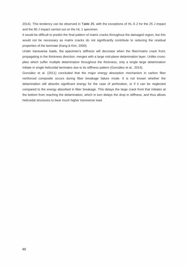
60
2014). This tendency can be observed in Table 25, with the exceptions of HL-S 2 for the 25 J impact
and the 80 J impact carried out on the HL 1 specimen.
It would be difficult to predict the final pattern of matrix cracks throughout the damaged region, but this
would not be necessary as matrix cracks do not significantly contribute to reducing the residual
properties of the laminate (Kang & Kim, 2000).
Under transverse loads, the specimen’s stiffness will decrease when the fiber/matrix crack front,
propagating in the thickness direction, merges with a large mid-plane delamination layer. Unlike cross-
plies which suffer multiple delamination throughout the thickness, only a single large delamination
initiate in single helicoidal laminates due to its stiffness pattern (González et al., 2014).
González et al. (2011) concluded that the major energy absorption mechanism in carbon fiber
reinforced composite occurs during fiber breakage failure mode. It is not known whether the
delamination still absorbs significant energy for the case of perforation, or if it can be neglected
compared to the energy absorbed in fiber breakage. This delays the large crack front that initiates at
the bottom from reaching the delamination, which in turn delays the drop in stiffness, and thus allows
helicoidal structures to bear much higher transverse load.
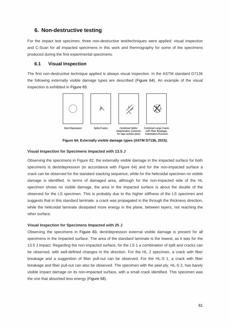
61
6. Non-destructive testing
For the impact test specimen, three non-destructive test/techniques were applied: visual inspection
and C-Scan for all impacted specimens in this work and thermography for some of the specimens
produced during the first experimental specimens.
6.1 Visual Inspection
The first non-destructive technique applied is always visual inspection. In the ASTM standard D7136
the following externally visible damage types are described (Figure 64). An example of the visual
inspection is exhibited in Figure 65.
Figure 64: Externally visible damage types (ASTM D7136, 2015).
Visual Inspection for Specimens Impacted with 13.5 J
Observing the specimens in Figure 82, the externally visible damage in the impacted surface for both
specimens is dent/depression (in accordance with Figure 64) and for the non-impacted surface a
crack can be observed for the standard stacking sequence, while for the helicoidal specimen no visible
damage is identified. In terms of damaged area, although for the non-impacted side of the HL
specimen shows no visible damage, the area in the impacted surface is about the double of the
observed for the LS specimen. This is probably due to the higher stiffness of the LS specimen and
suggests that in this standard laminate, a crack was propagated in the through the thickness direction,
while the helicoidal laminate dissipated more energy in the plane, between layers, not reaching the
other surface.
Visual Inspection for Specimens Impacted with 25 J
Observing the specimens in Figure 83, dent/depression external visible damage is present for all
specimens in the impacted surface. The area of the standard laminate is the lowest, as it was for the
13.5 J impact. Regarding the non-impacted surface, for the LS 1 a combination of split and cracks can
be observed, with well-defined changes in the direction. For the HL 2 specimen, a crack with fiber
breakage and a suggestion of fiber pull-out can be observed. For the HL-S 1, a crack with fiber
breakage and fiber pull-out can also be observed. The specimen with the peel-ply, HL-S 2, has barely
visible impact damage on its non-impacted surface, with a small crack identified. This specimen was
the one that absorbed less energy (Figure 58).

62
Visual Inspection for Specimens Impacted with 40 J
Observing the specimens in Figure 84, indentation/puncture with delamination is suggested for both
impacted surfaces, more pronounced for HL-S 1 but more severe in terms of fiber breakage for HL-S
2, although the similar damage area. For the non-impacted surface, both present large cracks with
fiber breakage, with the difference that HL-S 1 has a more extensive damage area and HL-S 2 has
more pronounced fiber breakage and pull-out.
Visual Inspection for Specimens Impacted with 80 J
Observing the specimens in Figure 85, it is clear that all specimens present combined large cracks,
with fiber breakage derived from the puncture that achieved perforation. On the non-impacted area,
petaling is observed. This failure mode is described in (Safri et al., 2014) and occurs when the tensile
strength is exceeded at the rear side of the target and it develops a star-shaped crack around the tip
of the impactor. The referred petals are formed when the layers are pushed by the motion of the
impactor.
Figure 65: Visual inspection for HL-1 specimen impacted with 80 J.
6.2 C-Scan
Principles
C-Scan is a test based on ultrasonic19
waves, generated by piezoelectric transducers which convert
an oscillating applied voltage into mechanical vibration. The frequency induces vibrations that are
transmitted into the test material by means of a coupling medium, such as water (Fahr, 1992).
The ultrasonic waves are disturbed when differences in acoustic impedance occur. Acoustic
impedance of a material is the product of its density times the acoustic velocity across it.
19
Ultrasound is any sound with a frequency over the superior limit of the human ear, which range is from around
20 to 20 000 Hz. Although any frequency above 20 000 Hz is considered ultrasound, for ultrasonic inspection, this
frequency is usually in the range of 2-10 MHz.

63
In an elastic material, the propagation is transmitted by the displacement of material particles. There
are two basic types of waves propagate in the bulk of a material: longitudinal (compressional) and
transverse (shear).
Figure 66: Single element transducer – adapted from (Olympus).
The test is performed by transmitting continuous waves of sound into the object and capturing the
reflected sounds. The reflected sounds paint an image of the object, and in this manner determine the
size and shape of the defects – differences in acoustic impedance. Kessler (Kessler, 2004) affirmed
that one main disadvantage of the conventional ultrasound test is that, in order to gain a good picture
of the material layers, the measurement device has to be in contact with the material in order to
minimize impedance. Newer technology can enable non-contact ultrasonic testing techniques to be
used. Different types of ultrasonic testers currently exist, such as simple devices that give only a
digital readout of the thickness, to complex systems that show the size and shape of the defects.
What is seen in the C-Scan is a projection of the delamination areas over the structure thickness.
Therefore, the delaminations which are close to the impacted surface may hide deeper delaminations.
However, larger delaminations are often in plies far from the impacted surface and can usually be
detected. Delaminations present a so-called peanut shape and the superposition of these
delaminations yields to a circular projected area (González et al., 2011).
As explained in the (Olympus) website, the typical beam of a transducer’s disc is often considered as
an energy column - Figure 67 - from the active element area that expands in diameter and,
progressively, dissipates.
Figure 67: Typical transducer beam (Olympus).
The beam profile is actually more complex, with pressure gradients in both axial and transversal
directions. In Figure 68, on the beam profile, the red color represents the areas with higher energy,
while the green and yellow colors represent areas of lower energy.
Figure 68: Representation of the pressure gradients of beam (Olympus).
The pulse-echo method, which is the most widely used ultrasonic method, involves the detection of
echoes produced when an ultrasonic pulse is reflected from a discontinuity or an interface of a test
piece. This method is often used for flaws location and thickness measurements.
C-scan displays the echoes from the internal portions of the test pieces as a function of the position of
each reflecting interface, within an area. Flaws are shown on a read-out, super-imposed on a plane
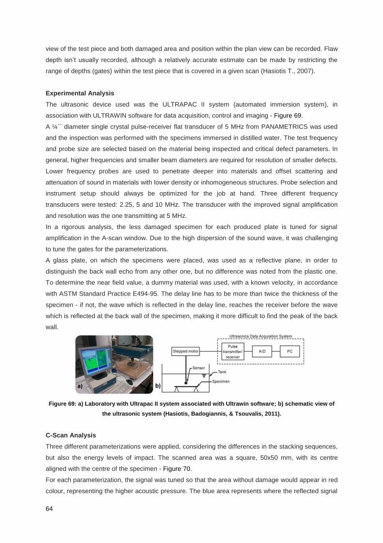
64
view of the test piece and both damaged area and position within the plan view can be recorded. Flaw
depth isn’t usually recorded, although a relatively accurate estimate can be made by restricting the
range of depths (gates) within the test piece that is covered in a given scan (Hasiotis T., 2007).
Experimental Analysis
The ultrasonic device used was the ULTRAPAC II system (automated immersion system), in
association with ULTRAWIN software for data acquisition, control and imaging - Figure 69.
A ¼΄΄ diameter single crystal pulse-receiver flat transducer of 5 MHz from PANAMETRICS was used
and the inspection was performed with the specimens immersed in distilled water. The test frequency
and probe size are selected based on the material being inspected and critical defect parameters. In
general, higher frequencies and smaller beam diameters are required for resolution of smaller defects.
Lower frequency probes are used to penetrate deeper into materials and offset scattering and
attenuation of sound in materials with lower density or inhomogeneous structures. Probe selection and
instrument setup should always be optimized for the job at hand. Three different frequency
transducers were tested: 2.25, 5 and 10 MHz. The transducer with the improved signal amplification
and resolution was the one transmitting at 5 MHz.
In a rigorous analysis, the less damaged specimen for each produced plate is tuned for signal
amplification in the A-scan window. Due to the high dispersion of the sound wave, it was challenging
to tune the gates for the parameterizations.
A glass plate, on which the specimens were placed, was used as a reflective plane, in order to
distinguish the back wall echo from any other one, but no difference was noted from the plastic one.
To determine the near field value, a dummy material was used, with a known velocity, in accordance
with ASTM Standard Practice E494-95. The delay line has to be more than twice the thickness of the
specimen - if not, the wave which is reflected in the delay line, reaches the receiver before the wave
which is reflected at the back wall of the specimen, making it more difficult to find the peak of the back
wall.
Figure 69: a) Laboratory with Ultrapac II system associated with Ultrawin software; b) schematic view of
the ultrasonic system (Hasiotis, Badogiannis, & Tsouvalis, 2011).
C-Scan Analysis
Three different parameterizations were applied, considering the differences in the stacking sequences,
but also the energy levels of impact. The scanned area was a square, 50x50 mm, with its centre
aligned with the centre of the specimen - Figure 70.
For each parameterization, the signal was tuned so that the area without damage would appear in red
colour, representing the higher acoustic pressure. The blue area represents where the reflected signal
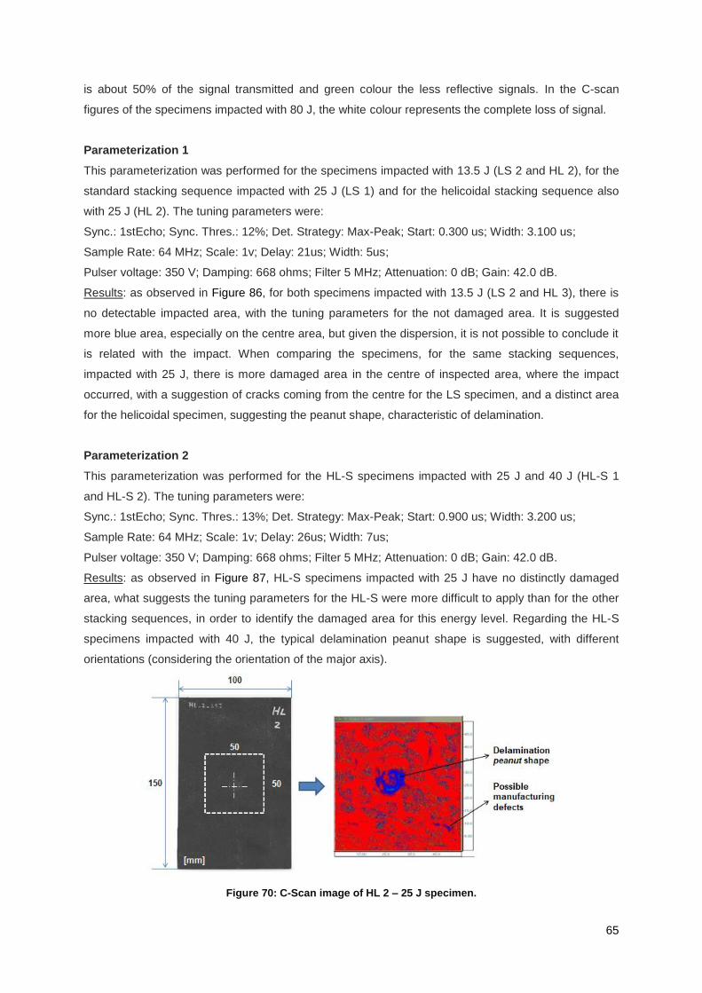
65
is about 50% of the signal transmitted and green colour the less reflective signals. In the C-scan
figures of the specimens impacted with 80 J, the white colour represents the complete loss of signal.
Parameterization 1
This parameterization was performed for the specimens impacted with 13.5 J (LS 2 and HL 2), for the
standard stacking sequence impacted with 25 J (LS 1) and for the helicoidal stacking sequence also
with 25 J (HL 2). The tuning parameters were:
Sync.: 1stEcho; Sync. Thres.: 12%; Det. Strategy: Max-Peak; Start: 0.300 us; Width: 3.100 us;
Sample Rate: 64 MHz; Scale: 1v; Delay: 21us; Width: 5us;
Pulser voltage: 350 V; Damping: 668 ohms; Filter 5 MHz; Attenuation: 0 dB; Gain: 42.0 dB.
Results: as observed in Figure 86, for both specimens impacted with 13.5 J (LS 2 and HL 3), there is
no detectable impacted area, with the tuning parameters for the not damaged area. It is suggested
more blue area, especially on the centre area, but given the dispersion, it is not possible to conclude it
is related with the impact. When comparing the specimens, for the same stacking sequences,
impacted with 25 J, there is more damaged area in the centre of inspected area, where the impact
occurred, with a suggestion of cracks coming from the centre for the LS specimen, and a distinct area
for the helicoidal specimen, suggesting the peanut shape, characteristic of delamination.
Parameterization 2
This parameterization was performed for the HL-S specimens impacted with 25 J and 40 J (HL-S 1
and HL-S 2). The tuning parameters were:
Sync.: 1stEcho; Sync. Thres.: 13%; Det. Strategy: Max-Peak; Start: 0.900 us; Width: 3.200 us;
Sample Rate: 64 MHz; Scale: 1v; Delay: 26us; Width: 7us;
Pulser voltage: 350 V; Damping: 668 ohms; Filter 5 MHz; Attenuation: 0 dB; Gain: 42.0 dB.
Results: as observed in Figure 87, HL-S specimens impacted with 25 J have no distinctly damaged
area, what suggests the tuning parameters for the HL-S were more difficult to apply than for the other
stacking sequences, in order to identify the damaged area for this energy level. Regarding the HL-S
specimens impacted with 40 J, the typical delamination peanut shape is suggested, with different
orientations (considering the orientation of the major axis).
Figure 70: C-Scan image of HL 2 – 25 J specimen.
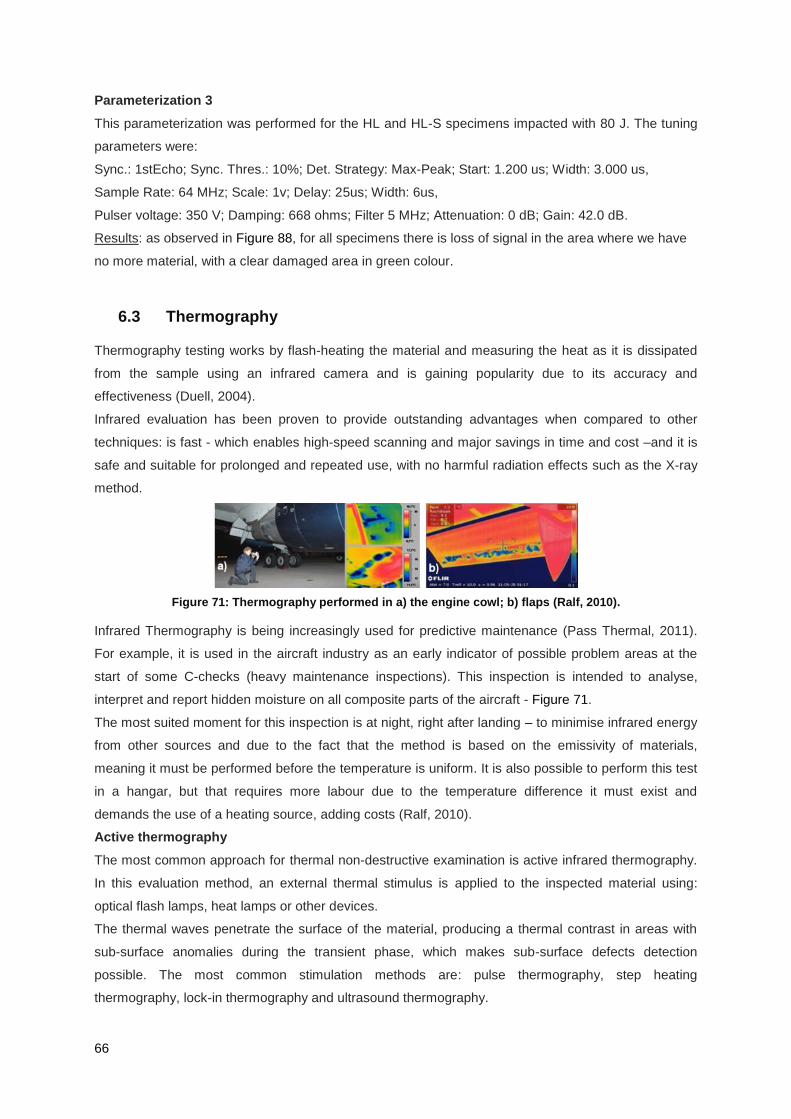
66
Parameterization 3
This parameterization was performed for the HL and HL-S specimens impacted with 80 J. The tuning
parameters were:
Sync.: 1stEcho; Sync. Thres.: 10%; Det. Strategy: Max-Peak; Start: 1.200 us; Width: 3.000 us,
Sample Rate: 64 MHz; Scale: 1v; Delay: 25us; Width: 6us,
Pulser voltage: 350 V; Damping: 668 ohms; Filter 5 MHz; Attenuation: 0 dB; Gain: 42.0 dB.
Results: as observed in Figure 88, for all specimens there is loss of signal in the area where we have
no more material, with a clear damaged area in green colour.
6.3 Thermography
Thermography testing works by flash-heating the material and measuring the heat as it is dissipated
from the sample using an infrared camera and is gaining popularity due to its accuracy and
effectiveness (Duell, 2004).
Infrared evaluation has been proven to provide outstanding advantages when compared to other
techniques: is fast - which enables high-speed scanning and major savings in time and cost –and it is
safe and suitable for prolonged and repeated use, with no harmful radiation effects such as the X-ray
method.
Figure 71: Thermography performed in a) the engine cowl; b) flaps (Ralf, 2010).
Infrared Thermography is being increasingly used for predictive maintenance (Pass Thermal, 2011).
For example, it is used in the aircraft industry as an early indicator of possible problem areas at the
start of some C-checks (heavy maintenance inspections). This inspection is intended to analyse,
interpret and report hidden moisture on all composite parts of the aircraft - Figure 71.
The most suited moment for this inspection is at night, right after landing – to minimise infrared energy
from other sources and due to the fact that the method is based on the emissivity of materials,
meaning it must be performed before the temperature is uniform. It is also possible to perform this test
in a hangar, but that requires more labour due to the temperature difference it must exist and
demands the use of a heating source, adding costs (Ralf, 2010).
Active thermography
The most common approach for thermal non-destructive examination is active infrared thermography.
In this evaluation method, an external thermal stimulus is applied to the inspected material using:
optical flash lamps, heat lamps or other devices.
The thermal waves penetrate the surface of the material, producing a thermal contrast in areas with
sub-surface anomalies during the transient phase, which makes sub-surface defects detection
possible. The most common stimulation methods are: pulse thermography, step heating
thermography, lock-in thermography and ultrasound thermography.
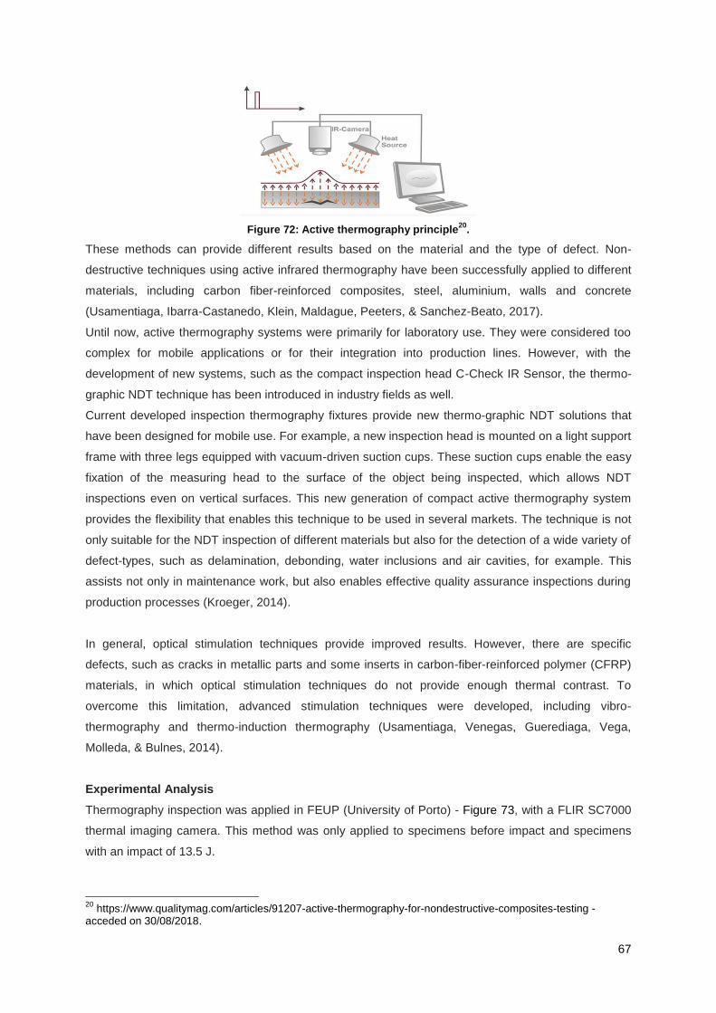
67
Figure 72: Active thermography principle20
.
These methods can provide different results based on the material and the type of defect. Non-
destructive techniques using active infrared thermography have been successfully applied to different
materials, including carbon fiber-reinforced composites, steel, aluminium, walls and concrete
(Usamentiaga, Ibarra-Castanedo, Klein, Maldague, Peeters, & Sanchez-Beato, 2017).
Until now, active thermography systems were primarily for laboratory use. They were considered too
complex for mobile applications or for their integration into production lines. However, with the
development of new systems, such as the compact inspection head C-Check IR Sensor, the thermo-
graphic NDT technique has been introduced in industry fields as well.
Current developed inspection thermography fixtures provide new thermo-graphic NDT solutions that
have been designed for mobile use. For example, a new inspection head is mounted on a light support
frame with three legs equipped with vacuum-driven suction cups. These suction cups enable the easy
fixation of the measuring head to the surface of the object being inspected, which allows NDT
inspections even on vertical surfaces. This new generation of compact active thermography system
provides the flexibility that enables this technique to be used in several markets. The technique is not
only suitable for the NDT inspection of different materials but also for the detection of a wide variety of
defect-types, such as delamination, debonding, water inclusions and air cavities, for example. This
assists not only in maintenance work, but also enables effective quality assurance inspections during
production processes (Kroeger, 2014).
In general, optical stimulation techniques provide improved results. However, there are specific
defects, such as cracks in metallic parts and some inserts in carbon-fiber-reinforced polymer (CFRP)
materials, in which optical stimulation techniques do not provide enough thermal contrast. To
overcome this limitation, advanced stimulation techniques were developed, including vibro-
thermography and thermo-induction thermography (Usamentiaga, Venegas, Guerediaga, Vega,
Molleda, & Bulnes, 2014).
Experimental Analysis
Thermography inspection was applied in FEUP (University of Porto) - Figure 73, with a FLIR SC7000
thermal imaging camera. This method was only applied to specimens before impact and specimens
with an impact of 13.5 J.
20
https://www.qualitymag.com/articles/91207-active-thermography-for-nondestructive-composites-testing - acceded on 30/08/2018.
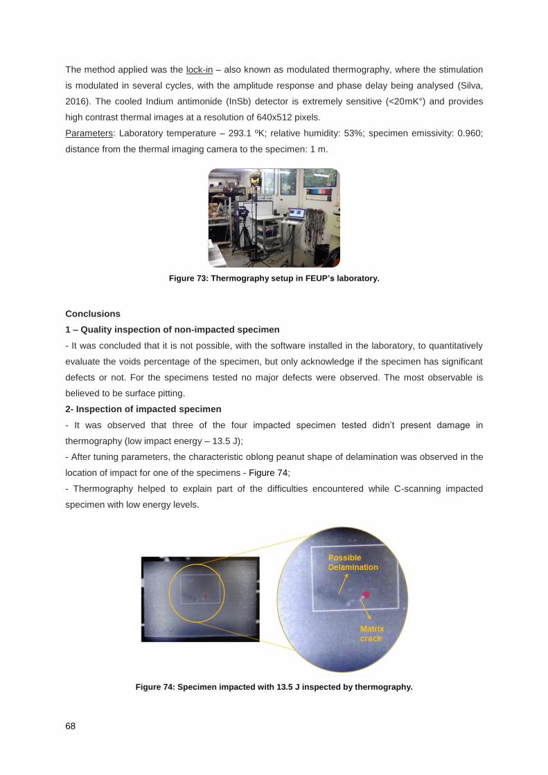
68
The method applied was the lock-in – also known as modulated thermography, where the stimulation
is modulated in several cycles, with the amplitude response and phase delay being analysed (Silva,
2016). The cooled Indium antimonide (InSb) detector is extremely sensitive (<20mK°) and provides
high contrast thermal images at a resolution of 640x512 pixels.
Parameters: Laboratory temperature – 293.1 ºK; relative humidity: 53%; specimen emissivity: 0.960;
distance from the thermal imaging camera to the specimen: 1 m.
Figure 73: Thermography setup in FEUP’s laboratory.
Conclusions
1 – Quality inspection of non-impacted specimen
- It was concluded that it is not possible, with the software installed in the laboratory, to quantitatively
evaluate the voids percentage of the specimen, but only acknowledge if the specimen has significant
defects or not. For the specimens tested no major defects were observed. The most observable is
believed to be surface pitting.
2- Inspection of impacted specimen
- It was observed that three of the four impacted specimen tested didn’t present damage in
thermography (low impact energy – 13.5 J);
- After tuning parameters, the characteristic oblong peanut shape of delamination was observed in the
location of impact for one of the specimens - Figure 74;
- Thermography helped to explain part of the difficulties encountered while C-scanning impacted
specimen with low energy levels.
Figure 74: Specimen impacted with 13.5 J inspected by thermography.
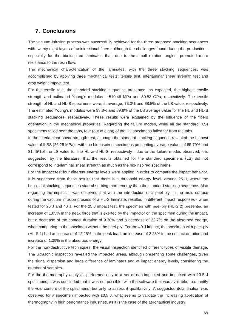
69
7. Conclusions
The vacuum infusion process was successfully achieved for the three proposed stacking sequences
with twenty-eight layers of unidirectional fibers, although the challenges found during the production -
especially for the bio-inspired laminates that, due to the small rotation angles, promoted more
resistance to the resin flow.
The mechanical characterization of the laminates, with the three stacking sequences, was
accomplished by applying three mechanical tests: tensile test, interlaminar shear strength test and
drop weight impact test.
For the tensile test, the standard stacking sequence presented, as expected, the highest tensile
strength and estimated Young’s modulus – 510.46 MPa and 30.53 GPa, respectively. The tensile
strength of HL and HL-S specimens were, in average, 76.3% and 68.5% of the LS value, respectively.
The estimated Young’s modulus were 93.8% and 89.8% of the LS average value for the HL and HL-S
stacking sequences, respectively. These results were explained by the influence of the fibers
orientation in the mechanical properties. Regarding the failure modes, while all the standard (LS)
specimens failed near the tabs, four (out of eight) of the HL specimens failed far from the tabs.
In the interlaminar shear strength test, although the standard stacking sequence revealed the highest
value of ILSS (26.25 MPa) - with the bio-inspired specimens presenting average values of 85.79% and
81.45%of the LS value for the HL and HL-S, respectively - due to the failure modes observed, it is
suggested, by the literature, that the results obtained for the standard specimens (LS) did not
correspond to interlaminar shear strength as much as the bio-inspired specimens.
For the impact test four different energy levels were applied in order to compare the impact behavior.
It is suggested from these results that there is a threshold energy level, around 25 J, where the
helicoidal stacking sequences start absorbing more energy than the standard stacking sequence. Also
regarding the impact, it was observed that with the introduction of a peel ply, in the mold surface
during the vacuum infusion process of a HL-S laminate, resulted in different impact responses - when
tested for 25 J and 40 J. For the 25 J impact test, the specimen with peel-ply (HL-S 2) presented an
increase of 1.85% in the peak force that is exerted by the impactor on the specimen during the impact,
but a decrease of the contact duration of 9.30% and a decrease of 22.7% on the absorbed energy,
when comparing to the specimen without the peel-ply. For the 40 J impact, the specimen with peel-ply
(HL-S 1) had an increase of 12.25% in the peak load, an increase of 2.23% in the contact duration and
increase of 1.39% in the absorbed energy.
For the non-destructive techniques, the visual inspection identified different types of visible damage.
The ultrasonic inspection revealed the impacted areas, although presenting some challenges, given
the signal dispersion and large difference of laminates and of impact energy levels, considering the
number of samples.
For the thermography analysis, performed only to a set of non-impacted and impacted with 13.5 J
specimens, it was concluded that it was not possible, with the software that was available, to quantify
the void content of the specimens, but only to assess it qualitatively. A suggested delamination was
observed for a specimen impacted with 13.5 J, what seems to validate the increasing application of
thermography in high performance industries, as it is the case of the aeronautical industry.

70
8. Future Work
This work was developed as part of a work package (WP2) of the MIT Portugal project – IAMAT. In
order to continue the mechanical characterization of bio-inspired composite structures, further work
will be performed in the referred work package:
- Determination of the elastic constants of the laminates;
- Compression After Impact (CAI) test to assess damage resistance;
- Laminates hybridization – use of more than one type of fibers, with lower aerial weight (veils),
in the same laminate – a method used nowadays to improve impact resistance.
It is also recommended:
- The introduction of multi-walled carbon nanotubes in CFRP laminates to evaluate the
interlaminar fracture toughness and impact resistance at different energy levels.

71
9. References
Abrate, S. (1991). Impact on Laminated Composite Materials. Applied Mechanics Review, 155-190
(44).
Adams, D. (2006, January). Unidirectional composite axial tensile specimens. Retrieved 2017, from
Composites World: https://www.compositesworld.com/articles/unidirectional-composite-axial-
tensile-specimens
Aerospace Structures @ UNSW. (2014, April). UNSW - Aerospace Structures - Composites.
Retrieved from Youtube: https://www.youtube.com/watch?v=V7bX4c9XWes
Airbus Technical Magazine. (2015). Printing the future with revolutionary Additive Layer
Manufacturing. Flight Airworthiness Support Technology, 8-9.
American Composites Manufacturers Association. (2009). Vacuum Infusion Process - Study Guide.
Arlington, VA, USA.
Angeloni - Fabrics Catalogue. High Tech Materials for Advanced Composites. Quarto D'Altino: G.
Angeloni Srl.
ASTM D2344. (2000). Standard Test Method for Short-Beam Strength of Polymer Matrix Composite
Materials and Their Laminates. 100 Barr Harbor Drive, West Conshohocken, PA 19428-2959,
United States.: ASTM International.
ASTM D3039. (2002). Standard Test Method for Tensile Properties of Polymer Matrix Composite
Materials. West Conshohocken, PA, 19428-2959 United States.
ASTM D7136. (2015). Standard Test Method for Measuring the Damage Resistance of a Fiber-
Reinforced Polymer Matrix Composite to a Drop-Weight Impact Event. West Conshohocken,
PA: ASTM International.
Bhudolia, S. K., Perrotey, P., & Joshi, S. C. (2017). Optimizing Polymer Infusion Process for Thin Ply
Textile Composites with Novel Matrix System. Materials (Basel).
Boeing. (2006). Boeing 787 from the Ground Up. Aero, pp. 19-26.
Boey, F., & Lye, S. (1992). Void reduction in autoclave processing of thermoset composites: Part 1:
High pressure effects on void reduction. Composites, Vol. 3, Issue 4, pp. 261-265.
Cardarelli, F. (2008). Materials Handbook. London: Springer.
Chia, S., Lee, S., Yeo, T., & Tan, K. (2001). Low Cost Composite Fabrication. Thirteen International
Conference on Composite Materials. Beijing.
Cognizant. (2015). Printing the Future: From Prototype to Production. Teaneck, NJ, USA: Cognizant.
Davies, G., & Zhang, X. (1995). Impact Damage Prediction in Carbon Composite Structures.
International Journal of Impact Engineering, Vol. 16, No. 1, pp. 149-170.
Derber, A. (2017, December 18). Out Of Autoclave, Into Production. Retrieved from MRO Network:
http://www.mro-network.com/manufacturing-distribution/out-autoclave-production
Dry Composites. (2013). Aerospace Looking to Dry Fiber/Infused Composites. Retrieved from Dry
Composites: http://www.drycomposites.com/aerospace-looking-to-dry-fiberinfused-
composites/

72
Duell, J. (2004). Impact Testing of Advanced Composites. In M. Kessler, Advanced Topics in
Characterization of Composites (pp. 97-111). Victoria, B.C., Canada: Trafford.
EASA. (2008). Bird Strike Damage & Windshield Bird Strike. Farnham, Surrey: ATKINS Limited and
Food & Environment Research Agency.
European Committee for Standardization. (1995). Aerospace Series - Carbon Fibre Reinforced
Plastics - Unidirectional Laminates - Tensile Test Parallel to the Fibre Direction. Brussels:
CEN Standard EN 2561.
Fahr, A. (1992). Ultrasonic C-Scan Inspection Of Composite Materials. Engineering Journal of Qatar
University, Vol. 5, pag. 201-222.
Farooq, U., & Myler, P. (2015). Prediction of load threshold of fibre-reinforced laminated composite
panels subjected to low velocity drop-weight impact using efficient data filtering techniques.
Results in Physics, Vol. 5, pp. 206-221.
Feraboli, P. J., Ireland, D. R., & Kedward, K. T. (2004). The Role of Force and Energy in Low Velocity
Impact Events. 45th Structures, Structural Dynamics & Materials Conference. Palm Springs,
CA.
Feraboli, P., & Kedward, K. (2003). Four-point bend interlaminar shear testing of uni- and multi-
directional carbon/epoxy composite systems. Composites.
Feraboli, P., & Kedward, K. (2004). In Search of True Interlaminar Shear Strength. American Society
for Composites/ American Society for Testing and Materials Committee D30. DEStech
Publications.
Ferreira, A., Nóvoa, R., & Marques, A. (2016). Multifunctional Material Systems: A state-of-the-art
review. Composite Structures, 3-35, Vol. 151.
Fibre Glast. Retrieved March 22, 2018, from Fibre Glast - Developments Corporation:
https://www.fibreglast.com/product/What-are-Unidirectional-Carbon-Fiber-
Fabrics/Learning_Center
Galliot, C., Rousseau, J., Valot, E., & Verchery, G. (2007). Influence of Stacking Sequences on the
Strenght of Composite Bonded Joints. 16th International Conference on Composite Materials.
Kyoto.
Ginzburg, D., Pinto, F., Iervolino, O., & Meo, M. (2016). Damage Tolerance of Bio-Inspired Helicoidal
Composites under Low Velocity Impact. Composite Structures.
González, E., Maimí, P., Camanho, P., Lopes, C., & Blanco, N. (2011). Effects of ply clustering in
laminated composite plates under low-velocity impact loading. Composites Science and
Technology.
González, E., Maimí, P., Sainz de Aja, J., Cruz, P., & Camanho, P. (2014). Effects of interply
hybridization on the damage resistance and tolerance of composite plates. Composite
Structures, pp. 319-331.
Grunenfelder, L., Suksangpanya, N., Salinas, C., Milliron, G., Yaraghi, N., Herrera, S., et al. (2014).
Bio-inspired impact-resistant composites. Acta Biomaterialia, 3997-4008, Vol. 10, Issue 9.
Halpin, J. C. (1992). Primer on Composite Materials Analysis. Boca Raton, FL 33487-2742: CRC
Press - Taylor & Francis Group.

73
Hasiotis T., B. E. (2007). Application of Ultrasonic C-Scan Techniques for Tracing Defects in
Laminated Composite Materials. 4th International Conference on NDT. Chania, Creete-
Greece.
Hasiotis, T., Badogiannis, E., & Tsouvalis, N. (2011). Application of Ultrasonic C-Scan Techniques for
Tracing Defects in Laminated Composite Materials. Journal of Mechanical Engineering, 192-
203 (3).
Irving, P., & Soutis, C. (2015). Polymer Composites in the Aerospace Industry. Cambridge: Elsevier.
ISO 14130. (1997). ISO 14130:1997 - Fibre-reinforced plastic composites — Determination of
apparent interlaminar shear strength by short-beam method. Brussels: European Committee
for Standardization.
Japanese Standards Association . (1988). Testing Method for Tensile Properties of Carbon Fibre
Reinforced Plastics. Tokyo: JIS K7073.
Kang, T., & Kim, C. (2000). Impact Energy Absorption Mechanism of Largely Deformable Composites
with Different Reinforcing Structures. Fibers and Polymers, Vol.1, No. 1, 45-54.
Kaw, A. K. (1997). Mechanics of Composite Materials. Boca Raton, Florida: CRC Press LLC.
Kennerley, J. (1998). Recycling fibres recovered from composite materials using a fluidised bed
process. Nottingham: University of Nottigham.
Kessler, M. R. (2004). Advanced Topics in Characterization of Composites. Trafford Publishing.
Kroeger, T. (2014, August 19). Thermographic inspection of composites. Retrieved from Materials
Today: https://www.materialstoday.com/composite-applications/features/thermographic-
inspection-of-composites/
Kühnel, M., & Kraus, T. (2016). The global CFRP market 2016. Augsburg: Carbon Composites.
Lawrence, B. D., & Emerson, R. P. (2012). A Comparison of Low-Velocity Impact and Quasi-Static
Indentation. Aberdeen Proving Ground, MD, USA: Army Research Laboratory.
Liu, J. L., & Tan, V. (2017). Improving Composite Laminates Through Biomimicry. ICCM-21. Xi'an,
China: International Committee on Composite Materials.
Luz, G., & Mano, J. (2009). Biomimetic design of materials and biomaterials inspired by the structure
of nacre. Philosophical Trans. of the Royal Society A - Mathematical, Physical and
Engineering Sciences.
Meyers, M., Chen, P., Lin, A., & Seki, Y. (2008). Biological materials: Structure and mechanical
properties. Progress in Materials Science, 1-206, 53.
Moura, M., Morais, A., & Magalhães, A. (2005). Materiais Compósitos - Materiais, Fabrico e
Comportamento Mecânico. Porto: Publindústria.
Ngern, N., & Shang, J. V. (2015). Impact Performance of Biomimetic Helicoidal Composite Plates.
International Conference on Composite Science and Technology. Lisboa: IDMEC.
Olsson, R., Donadon, M., & Falzon, B. (2006). Delamination threshold for dynamic impact on plates.
International Journal of Solids and Structures, Vol.43, Issue 10 pp. 3124-3141.
Olympus. Retrieved 2018, from https://www.olympus-ims.com/pt/

74
Pagano, N., & Pipes, R. (1971). The Influence of Stacking Sequence on Laminate Strength. Journal of
Composite Materials, pp. 50-57.
Paiva, J. M., Santos, A. D., & Rezende, M. C. (2009). Mechanical and Morphological
Characterizations of Carbon Fiber Fabric reinforced Epoxy Composites Used in Aeronautical
Field. Materials Research, Vol. 12, No. 3, 367-374.
Pass Thermal. (2011). Infrared Thermography for Maintenance. Retrieved 2018, from Youtube:
https://www.youtube.com/watch?v=MJczTk6_wcg
Patek, S. N., & Caldwell, R. L. (2005). Extreme impact and cavitation of a biological hammer: strike
forces of the peacock mantis shrimp Odontodactylus scyllarus. The Journal of Experimental
Biology, 3655-3664 (208).
Perez, M., Gil, L., & Oller, S. (2011). Non-destructive testing evaluation of low velocity impact damage
in carbon fiber-reinforced laminated composites. Ultragarsas (Ultrasound), Vol. 66, No. 2.
Pora, J. (2001). Composite Materials in the Airbus A380 - From History to Future -. Thirteenth
International Conference on Composite Materials (ICCM-13). Beijing.
Qiao, P., Yang, M., & Bobaru, F. (2008). Impact Mechanics and High Energy Absorbing Materials:
Review. Journal of Aerospace Engineering, pp. 235-248.
Ralf, G. (2010). Thermographic Inspections Used by Aircraft! Retrieved 2018, from Youtube:
https://www.youtube.com/watch?v=kfNA5beTUSw
Rhodes, M. B. (1980). Damage Tolerance Research on Composite Panels. NASA CP-2142.
Ribbans, B. (2015). Bioinspired Study On The Mechanical Performance Of Helicoidal Fiber Structures.
University of Vermont.
Safri, S., Sultan, M., Yidris, N., & Mustapha, F. (2014). Low Velocity and High Velocity Impact Test on
Composite Materials – A review. The International Journal Of Engineering And Science, 50-
60, Vol.3, Issue 9.
Sandlin, D. (2014). Retrieved from Youtube: https://www.youtube.com/watch?v=LXrxCT0NpHo
Sika. (2016). Biresin® CR83 - Composite Resin System.
Silva, A. (2016). Detection and Characterization of Defects in Composite Materials Using
Thermography. Porto: FEUP.
Sjoblom, P., Hartness, J. T., & Codell, T. M. (1988). On Low-Velocity Impact Testing of Composite
Materials. Journal of Composite Materials, 22 (1):30-52.
Sloan, J. (2016). Composites 101: Fibers and resins. Retrieved from Composites World:
https://www.compositesworld.com/articles/composites-101-fibers-and-resins
Smith, R. A. (2009). Composite defects and their detection. Materials Science and Engineering - Vol.
III.
Soto, A., González, E., Miamí, P., Escalera, M. d., Sainz de Aja, J., & Alvarez, E. (2018). Low velocity
impact and compression after impact simulation of thin ply laminates. Composites Part A:
Applied Science and Manufacturing, Vol. 109, pp. 413-427.
Soutis, C. (2005). Carbon fiber reinforced plastics in aircraft construction. Materials Science and
Engineering, 171-176.

75
Souza, G. P. (2003). Avaliação de Critérios de Falhas de Compósitos Poliméricos Reforçados
Aplicados a Vigas sob Carregamento de Flexão. São Paulo, Brazil: Escola de Engenharia de
São Carlos.
Spirit Aerosystems. (2017). Spirit AeroSystems Develops New Composites Manufacturing
Technology. Prestwick, Scotland: Spirit Aerosystems.
Sullivan, J. L., & Van Oene, H. (1986). An elasticity analysis for the generally and specially orthotropic
beams subjected to concentrated loads. Composites Science and Technology, Vol. 27, Issue
2, pp. 133-155.
Tanasa, F., & Zanoaga, M. (2013). Fiber-Reinforced Polymer Composites as a Structural Materials for
Aeronautics. International Conference of Scientific Paper Afases. Brasov, Romania.
Travesa, A. (2006). Simulation of delamination in composites under quasi-static and fatigue loading
using cohesive zone models. Girona: Universitat de Girona.
Turla, P., Kumar, S. S., Reddy, P. H., & Shekar, K. C. (2014). Interlaminar Shear Strength of Carbon
Fiber and Glass Fiber Reinforced Epoxy Matrix Hybrid Composite. International Journal of
Research in Engineering & Advanced Technology.
Usamentiaga, R., Ibarra-Castanedo, C., Klein, M., Maldague, X., Peeters, J., & Sanchez-Beato, A.
(2017). Nondestructive Evaluation of Carbon Fiber Bicycle Frames Using Infrared
Thermography. Sensors (Basel).
Usamentiaga, R., Venegas, P., Guerediaga, J., Vega, L., Molleda, J., & Bulnes, F. (2014). Infrared
Thermography for Temperature Measurement and Non-Destructive Testing. Sensors (Basel),
12305–12348, 14 (7).
Wang, C. Y., & Yew, C. H. (1990). Impact Damage in Composite Laminates. Computers & Structures,
976-982 (37:6).
Waterjets.org. (March 2018). Retrieved from https://waterjets.org/archive/getting-the-
most/tips/waterjet-machining-tolerances/
Weaver, J. C., Milliron, G. W., Miserez, A., Evans-Lutterodt, K., Herrera, S., Gallana, I., et al. (2012).
The Stomatopod Dactyl Club: A Formidable Damage-Tolerant Biological Hammer. Science,
1275-1280 - 336 (6086).
Wegst, U., & Ashby, M. (2004). The mechanical efficiency of natural materials. Philosophical
Magazine, 2167-2186 (84-21).
Whitney, J. M., & Browning, C. E. (1985). On short-beam shear tests for composite materials.
Experimental Mechanics, Vol. 25, Issue 3, pp 294-300.
Witik, R. A., Gaille, F., Teuscher, R., Ringwald, H., & Michaud, V. M.-A. (2012). Economic and
environmental assessment of alternative production methods for composite aircraft
components. Journal of Cleaner Production, p. 91-102, Vol. 29-30.
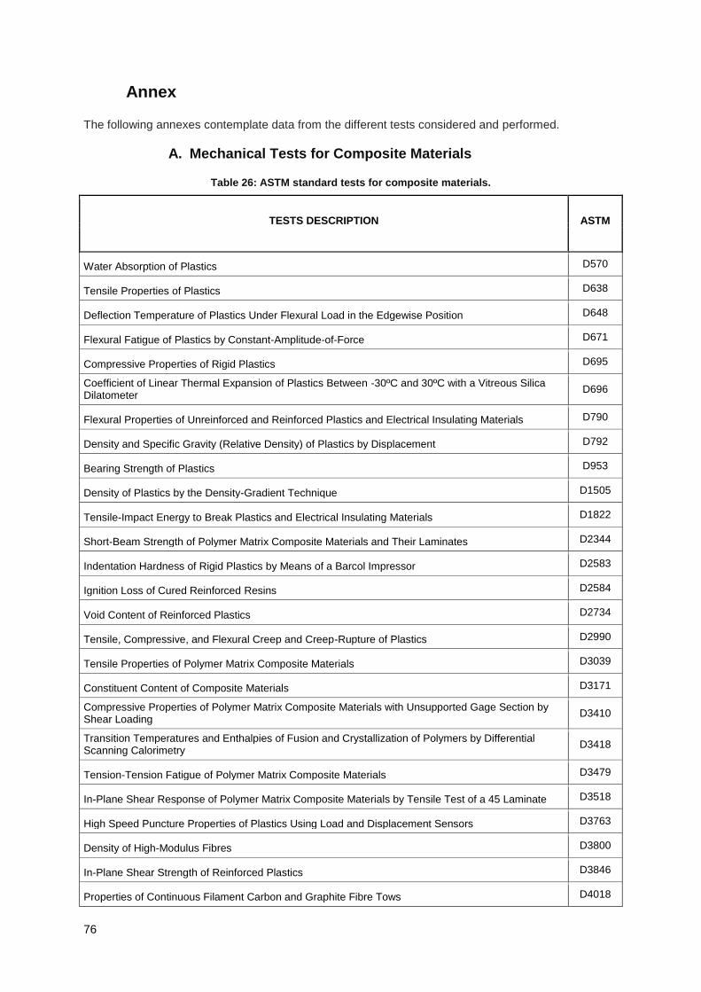
76
Annex
The following annexes contemplate data from the different tests considered and performed.
A. Mechanical Tests for Composite Materials
Table 26: ASTM standard tests for composite materials.
TESTS DESCRIPTION ASTM
Water Absorption of Plastics D570
Tensile Properties of Plastics D638
Deflection Temperature of Plastics Under Flexural Load in the Edgewise Position D648
Flexural Fatigue of Plastics by Constant-Amplitude-of-Force D671
Compressive Properties of Rigid Plastics D695
Coefficient of Linear Thermal Expansion of Plastics Between -30ºC and 30ºC with a Vitreous Silica Dilatometer
D696
Flexural Properties of Unreinforced and Reinforced Plastics and Electrical Insulating Materials D790
Density and Specific Gravity (Relative Density) of Plastics by Displacement D792
Bearing Strength of Plastics D953
Density of Plastics by the Density-Gradient Technique D1505
Tensile-Impact Energy to Break Plastics and Electrical Insulating Materials D1822
Short-Beam Strength of Polymer Matrix Composite Materials and Their Laminates D2344
Indentation Hardness of Rigid Plastics by Means of a Barcol Impressor D2583
Ignition Loss of Cured Reinforced Resins D2584
Void Content of Reinforced Plastics D2734
Tensile, Compressive, and Flexural Creep and Creep-Rupture of Plastics D2990
Tensile Properties of Polymer Matrix Composite Materials D3039
Constituent Content of Composite Materials D3171
Compressive Properties of Polymer Matrix Composite Materials with Unsupported Gage Section by Shear Loading
D3410
Transition Temperatures and Enthalpies of Fusion and Crystallization of Polymers by Differential Scanning Calorimetry
D3418
Tension-Tension Fatigue of Polymer Matrix Composite Materials D3479
In-Plane Shear Response of Polymer Matrix Composite Materials by Tensile Test of a 45 Laminate D3518
High Speed Puncture Properties of Plastics Using Load and Displacement Sensors D3763
Density of High-Modulus Fibres D3800
In-Plane Shear Strength of Reinforced Plastics D3846
Properties of Continuous Filament Carbon and Graphite Fibre Tows D4018

77
Thermal Oxidative Resistance of Carbon Fibres D4102
In-Plane Shear Properties of Polymer Matrix Composite Materials by the Rail Shear Method D4255
Plastics: Dynamic Mechanical Properties: Cure Behaviour D4473
Tensile Properties of Reinforced Thermosetting Plastics Using Straight-Sided Specimens D5083
Moisture Absorption Properties and Equilibrium Conditioning of Polymer Matrix Composite Materials D5229
Shear Properties of Composite Materials by the V-Notched Beam Method D5379
Mode I Interlaminar Fracture Toughness of Unidirectional Fibre-Reinforced Polymer Matrix Composite D5528
Open-Hole Tensile Strength of Polymer Matrix Composite Laminates D5766
Bearing Response of Polymer Matrix Composite Laminates D5961
Mode I Fatigue Delamination Growth Onset of Unidirectional Fibre-Reinforced Polymer Matrix Composites
D6115
Measuring the Damage Resistance of a FRP-Matrix Composite to a Concentrated Quasi-Isotropic Indentation Force
D6264
Flexural Properties of Unreinforced and Reinforced Plastics and Electrical Insulating Materials by Four-Point Bending
D6272
Measuring the Curved Beam Strength of a Fibre-Reinforced Polymer-Matrix Composite D6415
Test Method for Open-Hole Compressive Strength of Polymer Matrix Composite Laminates D6484
Compressive Properties of Polymer Matrix Composite Materials Using a Combined Loading Compression (CLC) Test Fixture
D6641
Mixed Mode I-Mode II Interlaminar Fracture Toughness of Unidirectional Fibre Reinforced Polymer Matrix Composites
D6671
Glass Transition Temperature of Polymer Matrix Composites by Dynamic Mechanical Analysis (DMA) D7028
Shear Properties of Composite Materials by V-Notched Rail Shear Method D7078
Measuring the Damage Resistance of a Fibre-Reinforced Polymer Matrix Composite to a Drop-Weight Impact Event
D7136
Compressive Residual Strength Properties of Damaged Polymer Matrix Composite Plates D7137
Flexural Properties of Polymer Matrix Composite Materials D7264
Through-Thickness Flatwise Tensile Strength and Elastic Modulus of a Fibre-Reinforced Polymer Matrix Composite Material
D7291
Measuring the Fastener Pull-Through Resistance of a Fibre-Reinforced Polymer Matrix Composite D7332
Cure Behaviour of Thermosetting Resins by Dynamic Mechanical Procedures using an Encapsulated Specimen Rheometer
D7750
Determination of the Mode II Interlaminar Fracture Toughness of Unidirectional Fibre-Reinforced Polymer Matrix Composites
D7905
Young's Modulus, Tangent Modulus and Chord Modulus E111
Poisson's Ratio at Room Temperature E132
Linear Thermal Expansion of Solid Materials With a Push-Rod Dilatometer E228
Performance Characteristics of Metallic Bonded Resistance Strain Gages E251
Determining Specific Heat Capacity by Differential Scanning Calorimetry E1269
Trans-laminar Fracture Toughness of Laminated and Pultruded Polymer Matrix Composite Materials E1922
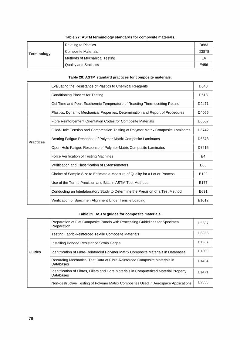
78
Table 27: ASTM terminology standards for composite materials.
Terminology
Relating to Plastics D883
Composite Materials D3878
Methods of Mechanical Testing E6
Quality and Statistics E456
Table 28: ASTM standard practices for composite materials.
Practices
Evaluating the Resistance of Plastics to Chemical Reagents D543
Conditioning Plastics for Testing D618
Gel Time and Peak Exothermic Temperature of Reacting Thermosetting Resins D2471
Plastics: Dynamic Mechanical Properties: Determination and Report of Procedures D4065
Fibre Reinforcement Orientation Codes for Composite Materials D6507
Filled-Hole Tension and Compression Testing of Polymer Matrix Composite Laminates D6742
Bearing Fatigue Response of Polymer Matrix Composite Laminates D6873
Open-Hole Fatigue Response of Polymer Matrix Composite Laminates D7615
Force Verification of Testing Machines E4
Verification and Classification of Extensometers E83
Choice of Sample Size to Estimate a Measure of Quality for a Lot or Process E122
Use of the Terms Precision and Bias in ASTM Test Methods E177
Conducting an Interlaboratory Study to Determine the Precision of a Test Method E691
Verification of Specimen Alignment Under Tensile Loading E1012
Table 29: ASTM guides for composite materials.
Guides
Preparation of Flat Composite Panels with Processing Guidelines for Specimen Preparation
D5687
Testing Fabric-Reinforced Textile Composite Materials D6856
Installing Bonded Resistance Strain Gages E1237
Identification of Fibre-Reinforced Polymer Matrix Composite Materials in Databases E1309
Recording Mechanical Test Data of Fibre-Reinforced Composite Materials in Databases
E1434
Identification of Fibres, Fillers and Core Materials in Computerized Material Property Databases
E1471
Non-destructive Testing of Polymer Matrix Composites Used in Aerospace Applications E2533
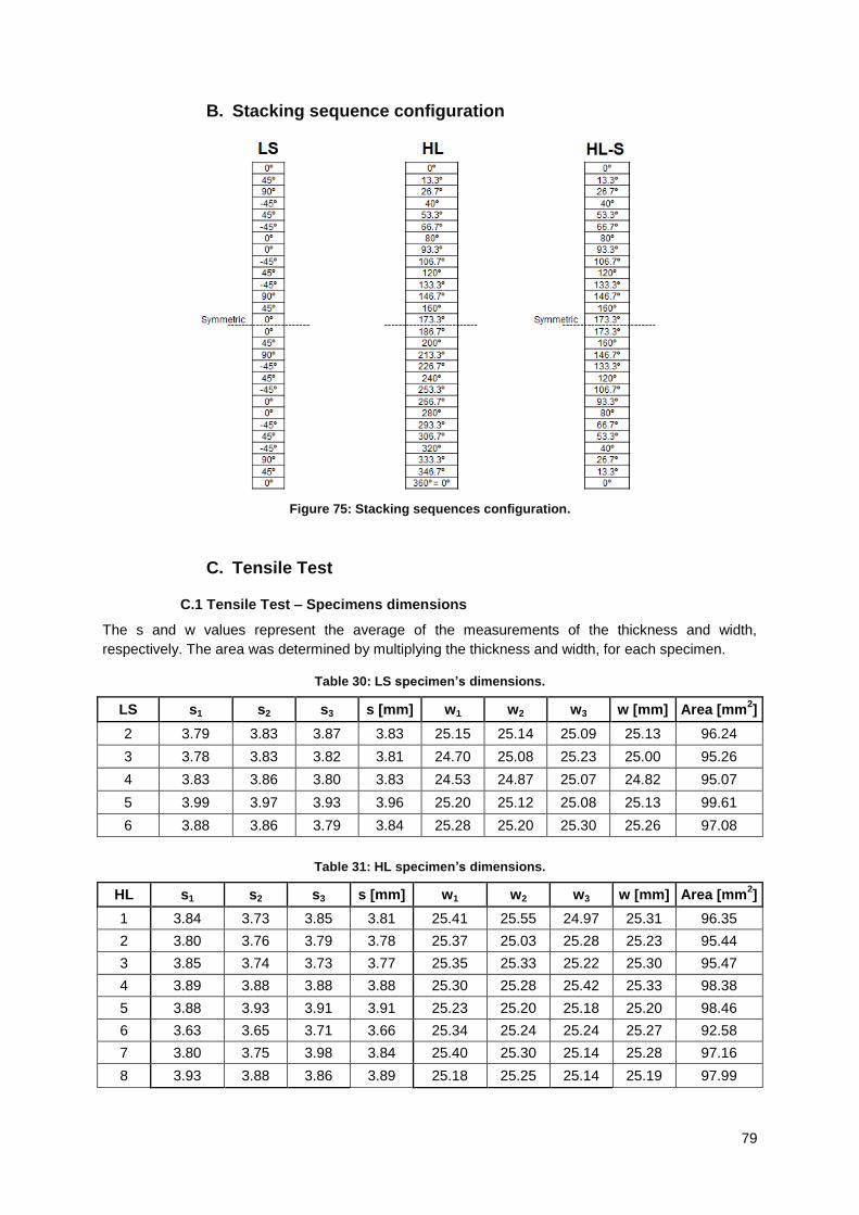
79
B. Stacking sequence configuration
Figure 75: Stacking sequences configuration.
C. Tensile Test
C.1 Tensile Test – Specimens dimensions
The s and w values represent the average of the measurements of the thickness and width,
respectively. The area was determined by multiplying the thickness and width, for each specimen.
Table 30: LS specimen’s dimensions.
LS s1 s2 s3 s [mm] w1 w2 w3 w [mm] Area [mm2]
2 3.79 3.83 3.87 3.83 25.15 25.14 25.09 25.13 96.24
3 3.78 3.83 3.82 3.81 24.70 25.08 25.23 25.00 95.26
4 3.83 3.86 3.80 3.83 24.53 24.87 25.07 24.82 95.07
5 3.99 3.97 3.93 3.96 25.20 25.12 25.08 25.13 99.61
6 3.88 3.86 3.79 3.84 25.28 25.20 25.30 25.26 97.08
Table 31: HL specimen’s dimensions.
HL s1 s2 s3 s [mm] w1 w2 w3 w [mm] Area [mm2]
1 3.84 3.73 3.85 3.81 25.41 25.55 24.97 25.31 96.35
2 3.80 3.76 3.79 3.78 25.37 25.03 25.28 25.23 95.44
3 3.85 3.74 3.73 3.77 25.35 25.33 25.22 25.30 95.47
4 3.89 3.88 3.88 3.88 25.30 25.28 25.42 25.33 98.38
5 3.88 3.93 3.91 3.91 25.23 25.20 25.18 25.20 98.46
6 3.63 3.65 3.71 3.66 25.34 25.24 25.24 25.27 92.58
7 3.80 3.75 3.98 3.84 25.40 25.30 25.14 25.28 97.16
8 3.93 3.88 3.86 3.89 25.18 25.25 25.14 25.19 97.99
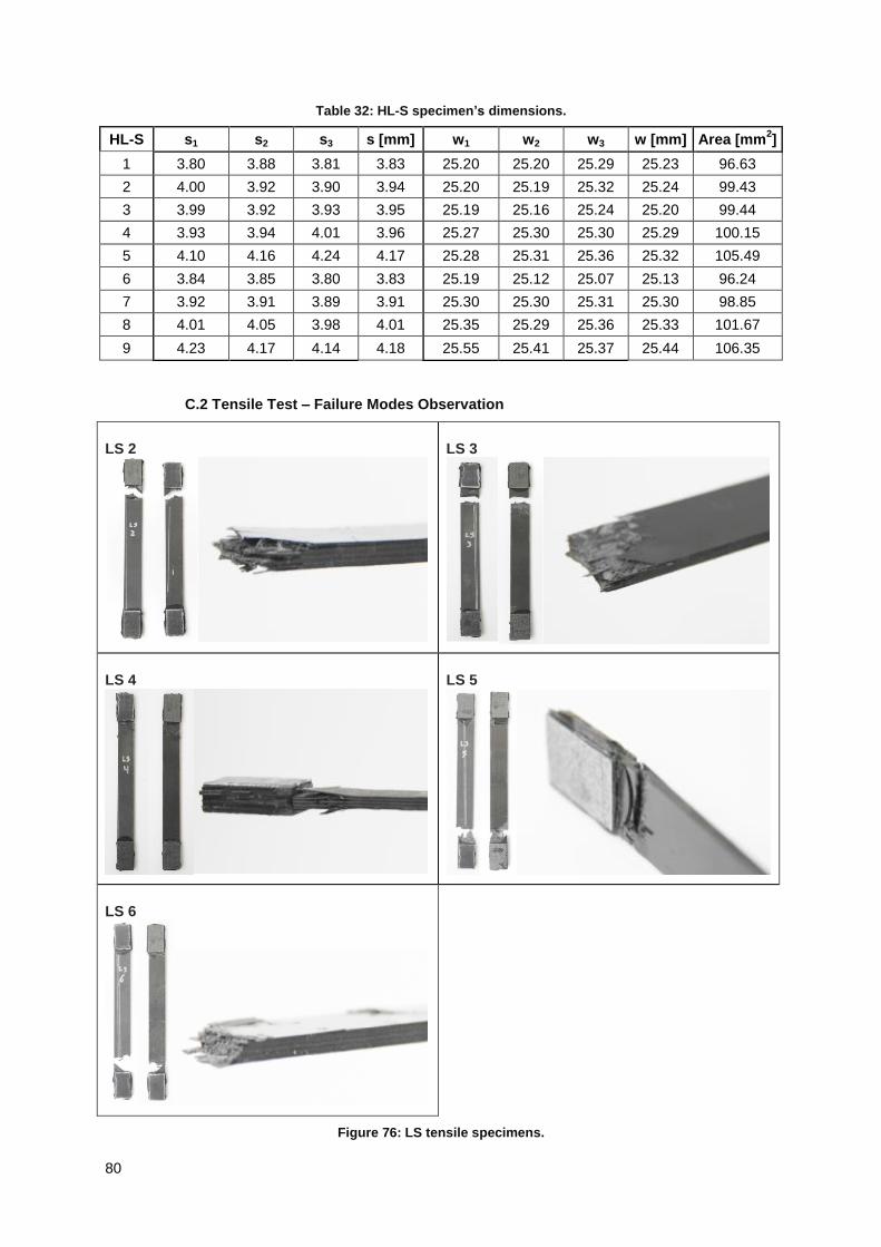
80
Table 32: HL-S specimen’s dimensions.
HL-S s1 s2 s3 s [mm] w1 w2 w3 w [mm] Area [mm2]
1 3.80 3.88 3.81 3.83 25.20 25.20 25.29 25.23 96.63
2 4.00 3.92 3.90 3.94 25.20 25.19 25.32 25.24 99.43
3 3.99 3.92 3.93 3.95 25.19 25.16 25.24 25.20 99.44
4 3.93 3.94 4.01 3.96 25.27 25.30 25.30 25.29 100.15
5 4.10 4.16 4.24 4.17 25.28 25.31 25.36 25.32 105.49
6 3.84 3.85 3.80 3.83 25.19 25.12 25.07 25.13 96.24
7 3.92 3.91 3.89 3.91 25.30 25.30 25.31 25.30 98.85
8 4.01 4.05 3.98 4.01 25.35 25.29 25.36 25.33 101.67
9 4.23 4.17 4.14 4.18 25.55 25.41 25.37 25.44 106.35
C.2 Tensile Test – Failure Modes Observation
LS 2
LS 3
LS 4
LS 5
LS 6
Figure 76: LS tensile specimens.
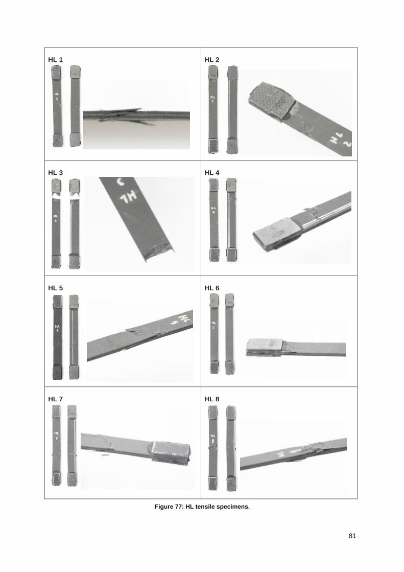
81
HL 1
HL 2
HL 3
HL 4
HL 5
HL 6
HL 7
HL 8
Figure 77: HL tensile specimens.

82
Figure 78: HL-S tensile specimens.
HL-S 1
HL-S 2
HL-S 3
HL-S 4
HL-S 5
HL-S 6
HL-S 8
HL-S 9
HL-S 10
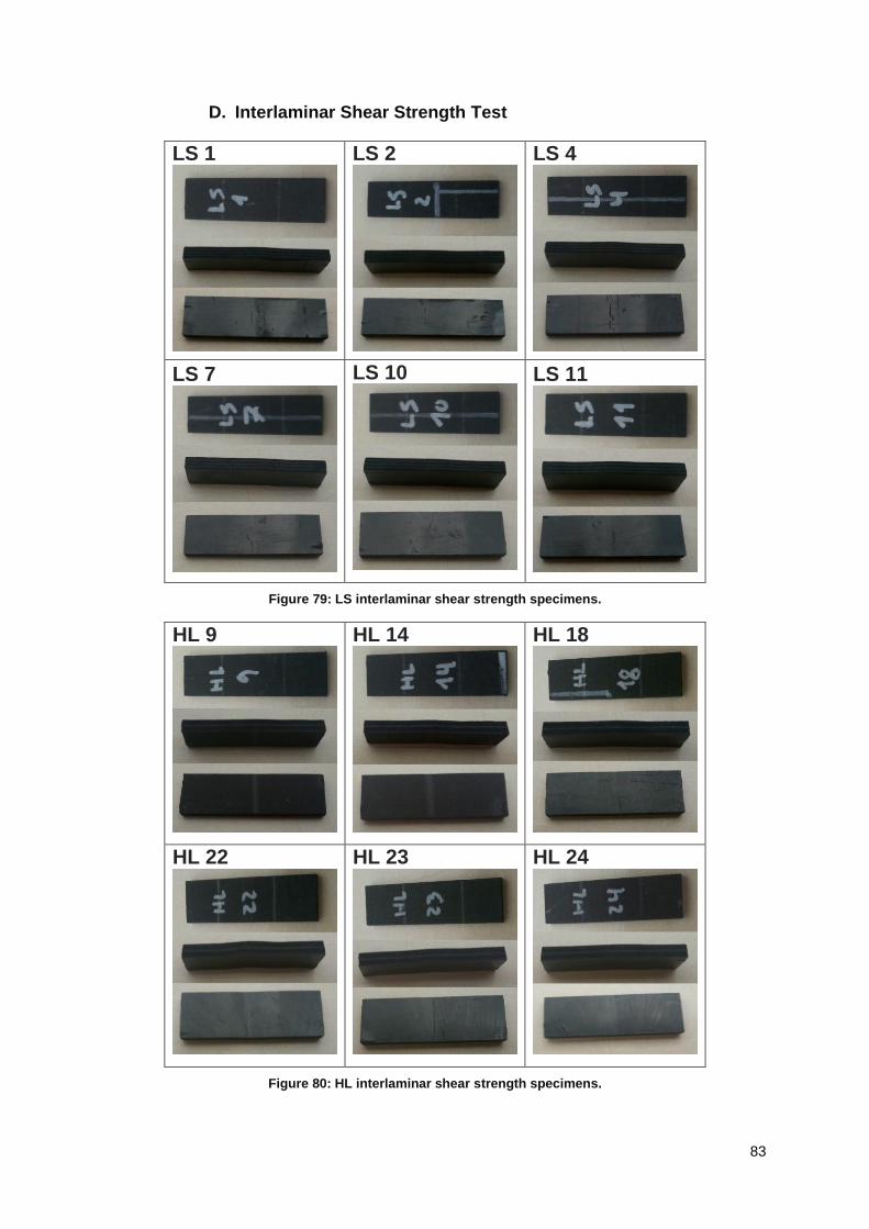
83
D. Interlaminar Shear Strength Test
LS 1
LS 2
LS 4
LS 7
LS 10
LS 11
Figure 79: LS interlaminar shear strength specimens.
HL 9
HL 14
HL 18
HL 22
HL 23
HL 24
Figure 80: HL interlaminar shear strength specimens.
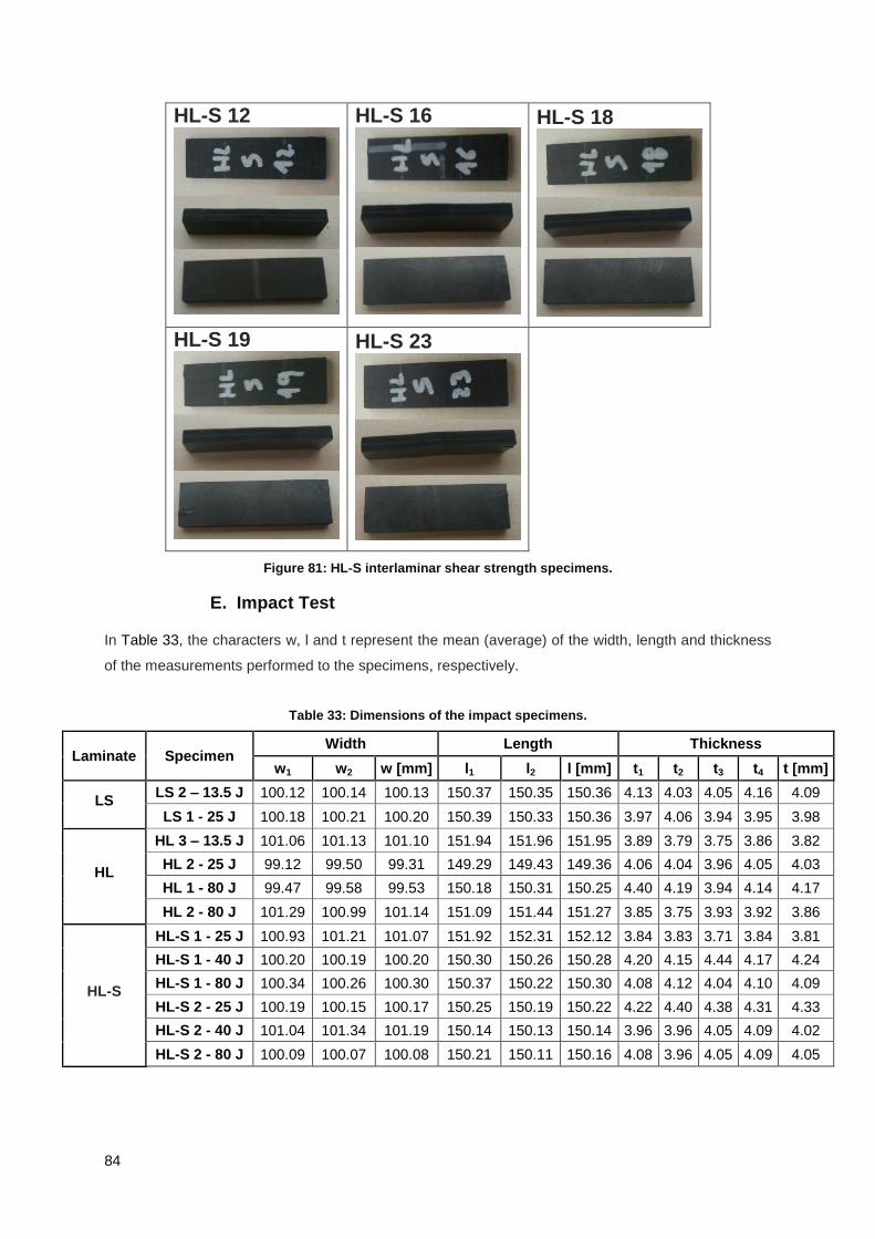
84
HL-S 12
HL-S 16
HL-S 18
HL-S 19
HL-S 23
Figure 81: HL-S interlaminar shear strength specimens.
E. Impact Test
In Table 33, the characters w, l and t represent the mean (average) of the width, length and thickness
of the measurements performed to the specimens, respectively.
Table 33: Dimensions of the impact specimens.
Laminate Specimen Width Length Thickness
w1 w2 w [mm] l1 l2 l [mm] t1 t2 t3 t4 t [mm]
LS LS 2 – 13.5 J 100.12 100.14 100.13 150.37 150.35 150.36 4.13 4.03 4.05 4.16 4.09
LS 1 - 25 J 100.18 100.21 100.20 150.39 150.33 150.36 3.97 4.06 3.94 3.95 3.98
HL
HL 3 – 13.5 J 101.06 101.13 101.10 151.94 151.96 151.95 3.89 3.79 3.75 3.86 3.82
HL 2 - 25 J 99.12 99.50 99.31 149.29 149.43 149.36 4.06 4.04 3.96 4.05 4.03
HL 1 - 80 J 99.47 99.58 99.53 150.18 150.31 150.25 4.40 4.19 3.94 4.14 4.17
HL 2 - 80 J 101.29 100.99 101.14 151.09 151.44 151.27 3.85 3.75 3.93 3.92 3.86
HL-S
HL-S 1 - 25 J 100.93 101.21 101.07 151.92 152.31 152.12 3.84 3.83 3.71 3.84 3.81
HL-S 1 - 40 J 100.20 100.19 100.20 150.30 150.26 150.28 4.20 4.15 4.44 4.17 4.24
HL-S 1 - 80 J 100.34 100.26 100.30 150.37 150.22 150.30 4.08 4.12 4.04 4.10 4.09
HL-S 2 - 25 J 100.19 100.15 100.17 150.25 150.19 150.22 4.22 4.40 4.38 4.31 4.33
HL-S 2 - 40 J 101.04 101.34 101.19 150.14 150.13 150.14 3.96 3.96 4.05 4.09 4.02
HL-S 2 - 80 J 100.09 100.07 100.08 150.21 150.11 150.16 4.08 3.96 4.05 4.09 4.05
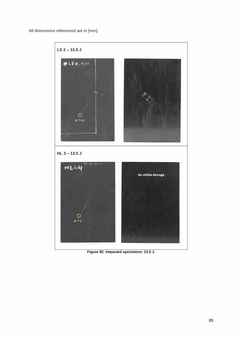
85
All dimensions referenced are in [mm].
Figure 82: Impacted specimens: 13.5 J.
LS 2 – 13.5 J
HL 3 – 13.5 J
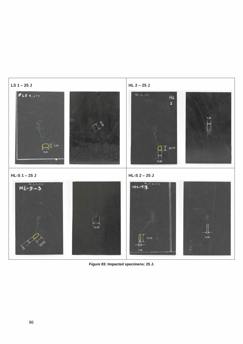
86
LS 1 – 25 J
HL 2 – 25 J
HL-S 1 – 25 J
HL-S 2 – 25 J
Figure 83: Impacted specimens: 25 J.
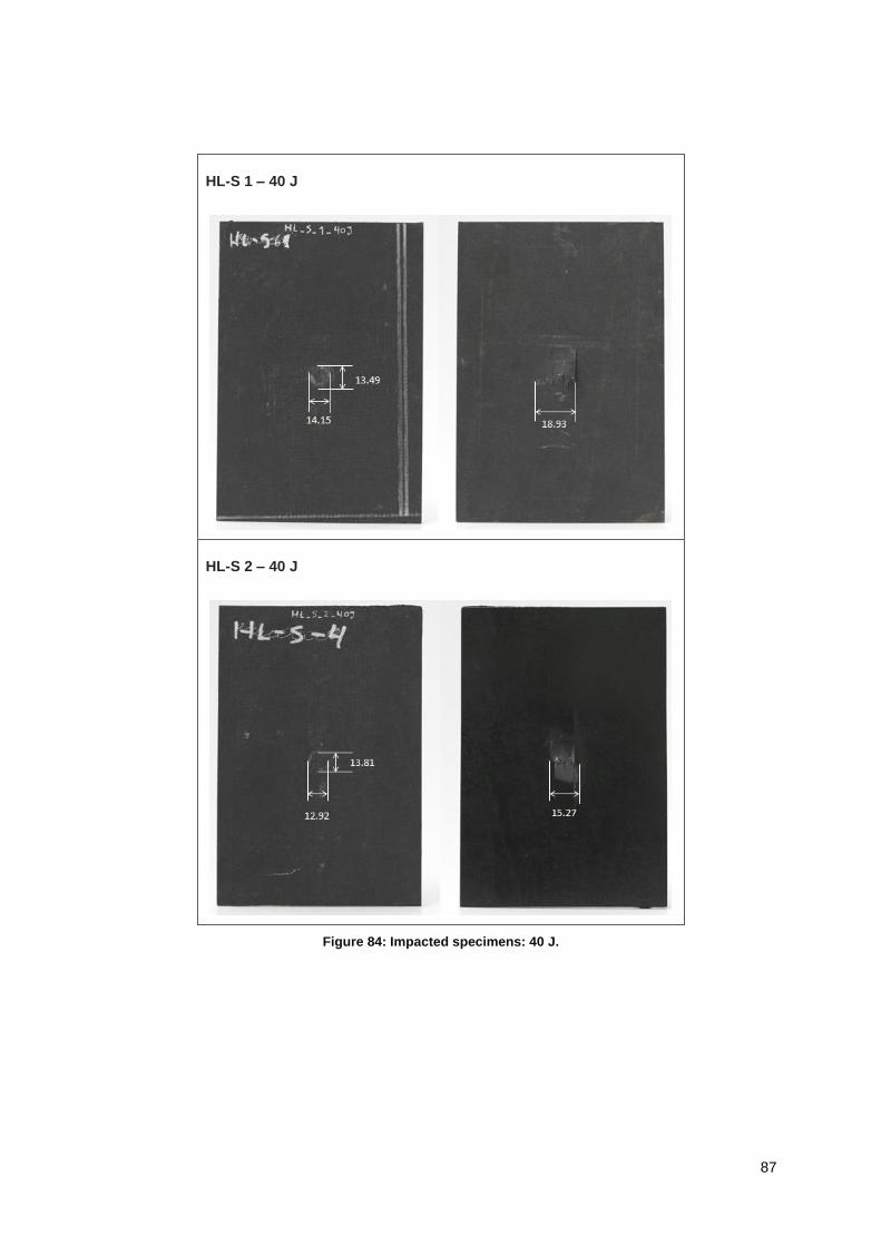
87
HL-S 1 – 40 J
HL-S 2 – 40 J
Figure 84: Impacted specimens: 40 J.
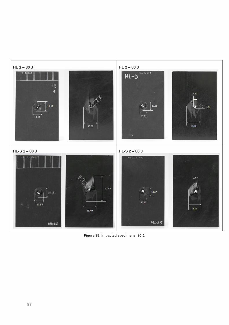
88
HL 1 – 80 J
HL 2 – 80 J
HL-S 1 – 80 J
HL-S 2 – 80 J
Figure 85: Impacted specimens: 80 J.
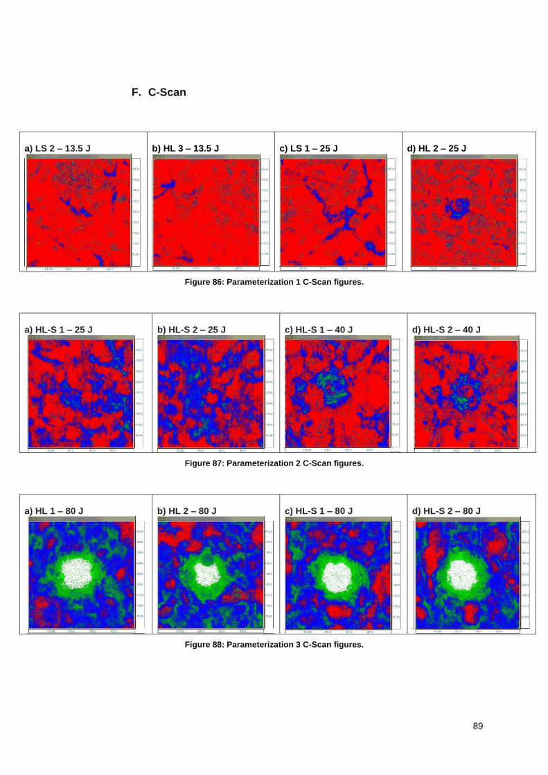
89
F. C-Scan
a) LS 2 – 13.5 J
b) HL 3 – 13.5 J
c) LS 1 – 25 J
d) HL 2 – 25 J
Figure 86: Parameterization 1 C-Scan figures.
a) HL-S 1 – 25 J
b) HL-S 2 – 25 J
c) HL-S 1 – 40 J
d) HL-S 2 – 40 J
Figure 87: Parameterization 2 C-Scan figures.
a) HL 1 – 80 J
b) HL 2 – 80 J
c) HL-S 1 – 80 J
d) HL-S 2 – 80 J
Figure 88: Parameterization 3 C-Scan figures.