mass conservation and singular multicomponent diffusion

IMPACT OF COMPUTING IN SCIENCE AND ENGINEERING 2, 73-97 ( 1990)

Mass Conservation and Singular Multicomponent Diffusion Algorithms

VINCENT GIOVANGIGLI

Centre de Mathkmatiques Appliqtkes, CA 756 du CNRS, Ecole Polytechnique, 91128 Palaiseau Cedex, France

Received January 4, 1990

Vincent Giovangigh, Mass Conservation and Singular Multicomponent Diffusion Algorithms, IMPACT of Computing in Science and Engineering 2, 73-97 ( 1990 )

We investigate mass conservation in multicomponent diffusion algorithms. Usual diffusion matrices are indeed singular, i.e., noninvertible, because of mass conservation constraints. A consequence is that when all mass fractions are treated as independent unknowns-a widely used approach in complex chemistry reacting flow solvers-artificial singularities may appear in the governing equations. These singularities arise, for instance, with species flux boundary conditions or with steady flows involving stagnation points. In these situations, the Jacobian matrices of the discrete governing equations are singular. Modifications of the usual diffusion algorithms are introduced to eliminate these singularities. These modifications, of course, do not change the actual values of the diffusion velocities. Only their mathematical expressions are changed. o ,990 Academic Press, Inc.

1. INTRODUCTION

The governing equations of multicomponent gaseous laminar reacting flows are the hydrodynamic equations derived from the kinetic theory of gases [l- 41. Derivation of these equations shows that at any time and at any point of the physical space, various mass conservation constraints are satisfied. Ex- amples of such constraints are the relations CkEB Yk = 1 between the species massfractions Y,,kES = (1,. . . , N8 } , where S is the set of species indices and N8 is the number of species; C kES & = 1 between the mole fractions &; CkEs Y,Vk = 0 between the species diffusion velocities V,; CkES dk = 0 between the diffusion driving force dk; and CkES Wk6& = 0 between the mass rate of production of the species wk Wk [l-3 1. These relations imply that the total mass conservation equation and the NS species mass conservation equations are linearly dependent. More specifically, the second-order species mass conservation equations sum up to the first-order total mass conservation

73 0899-8248/90 $3.00 Copyri!& 0 1990 by Academic Press, Inc. All rights of reproduction in any form reserved.

74 VINCENT GIOVANGIGLI

equation when written in conservative form whereas they sum up to zero when written in nonconservative form.

An attractive approach in problems having one species which is always in excess is therefore to consider only NC), - 1 species mass fractions as unknowns-aside from the mixture density p, the gas velocity u, and the temperature T-and to evaluate the excess species mass fraction by using the relation CktS Y, = 1. All of the mass conservation constraints are then automatically satisfied. However, this approach is not always feasible. In a typical diffusion flame, for instance, each species is deficient either on the fuel side or on the oxidant side and it is not accurate to evaluate one of the mass fractions by using CkES Y, = 1. An interesting approach still is to determine locally, at each computational cell, which species is in excess and to evaluate it by using CkES Y, = 1, but it requires solving a solution-dependent set of equations.

An alternate approach-widely used in complex chemistry reacting flow solvers-is to consider all the species mass fractions as independent unknowns [5-141. In this situation, it is important to analyze which of the mass constraints are automatically satisfied and which are consequences of the governing equations. Indeed the various diffusion algorithms expressing the diffusion velocities V, first show that the relation CkES Y, V, = 0 is always satisfied. Similarly the relation C kE6x I+‘+, = 0 between the chemical production rates wk is a consequence of their expression in terms of the reaction rates of progress, Usual relations expressing the mole fractions also yield the identity C&S X, = 1 so that the driving forces satisfy C&S dk = 0 under the approximation dk = VXk. On the other hand, the relation C&S Y, = I between the species mass fractions Yk must result from the conservation equations, the diffusion algorithm, and the boundary conditions. The equations for C&S Yk are indeed obtained by summing up the corresponding N,(- species equations. However, this latter set of equations may be artificially singular because of the constraints C&$ Yk vk = 0 and CkE$ Xk = 1 which also imply that diffusion matrices are noninvertible. These singularities may appear, for instance, with species flux boundary conditions or steady flows involving re- circulation zones or stagnation points. In these situations, the Jacobian matrices of the discrete governing equations are singular, i.e., noninvertible, and this may eventually lead to convergence difficulties of poor sensitivity information.

Elimination of the singularities requires modifying the usual diffusion algorithms. Modifications are proposed for three different diffusion algorithms. namely for the complex formalism of the kinetic theory of gases, for the Stefan-Maxwell equations, and for the Hirschfelder-Curtiss expressions with mass correctors [ l-3, 5, 7, 9, 12- 17 1. These modifications, of course, do not change the actual values of the diffusion velocities or the mole fractions. Only their mathematical expressions are changed.

SINGULAR MULTICOMPONENT DIFFUSION 75

The governing equations of gaseous laminar reacting flows which are needed in our analysis are presented in Section 2. In Section 3, different singularities are exhibited in the governing equations. The modified diffusion algorithms are introduced in Section 4 and the properties of the corresponding modified governing equations are discussed. Finally, numerical experiments are presented in Section 5.

2. GOVERNINGEQUATIONS

The governing equations of a gaseous laminar reacting flow are the equations for conservation of total mass, species mass, momentum, and energy. The corresponding dependent variables are the mixture density p; the N8 species mass fractions Y,, . . . , Y,,; the gas velocity u; and the absolute temperature T. These conservation equations must also be completed with the relations expressing thermodynamic properties, chemical production rates, and transport properties and suitable boundary conditions. Only the governing equations which are needed in our analysis are presented in the following.

2.1. Species Conservation Equations and Boundary Conditions

The species mass conservation equations in a gaseous laminar reacting flow may be written as

~5 + p(U’v)Yk = -v-(pykvk) + wkak, kE 8, (2.1)

where p is the density. Yk the mass fraction of the kth species, t the time, u the mass averaged flow velocity, vk the diffusion velocity of the kth species, wk the molecular weight of the kth species, Wk the molar production rate of the kth species, 8 = (1, . . . . Ng} the set of species indices, and Ns the number of species [ l-3 1. The total mass, momentum, and energy conservation equations and the law of state, which are not needed in our analysis, are not presented. Equations (2.1) are usually simplified according to the problem under study, e.g., steady flow or boundary layer flow.

Typical boundary conditions for the species mass fractions can be of Dir- ichlet, Neumann, or mixed type. Dirichlet boundary conditions are often involved with truncated infinite domains [ 61 and may be written

Y, = Y;, kE 8, (2.2)

where Y g denotes the specified mass fractions, which of course must be such that .&EB Yf = 1. Neumann boundary conditions often occur in symmetric problems [ 61 or truncated infinite domains [ 111 and lead to the relations


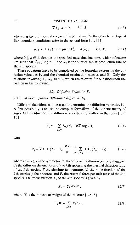
VYx* n = 0, k E s, (2.3 1

where n is the unit normal vector at the boundary. On the other hand, typical flux boundary conditions arise in the general form [ 11. 13 ]

pYfJu + v/o-n = pus nrfl+ w/g&, kE 8, (2.4)

where Yz, k E S, denotes the specified mass flux fractions, which of course are such that ZkES Y :! = 1, and iLlk is the surface molar production rate of the kth species.

These equations have to be completed by the formulas expressing the diffusion velocities V, and the chemical production rates @k and &k. Only the relations involving vk, Wk, and ijk which are relevant for our discussion are written in the following.

2.2. D(jiision Velocities Vk

2.2.1. hfU/tiCOmpOnent D@ision COt??CientS Dkl

Different algorithms can be used to determine the diffusion velocities V, . A first possibility is to use the complex formalism of the kinetic theory of gases. In this situation, the diffusion velocities are written in the form [ 1, 2. 151

vk = - 2 Dk,( d, + fl,v log r), ICE s

(2.5)

with

d, = VX, + (X1 - Y,) 7 + $ c Y,Y,(E;, - F,), rnES

(2.6)

where D = ( Dk,) is the symmetric multicomponent diffusion coefficient matrix, dk the diffusion driving force of the kth species, ok the thermal diffusion ratio of the kth species, T the absolute temperature, & the mole fraction of the kth species, p the pressure, and Fk the external force per unit mass of the kth species. The mole fraction & of the kth species is given by

(2.7)

where W is the molecular weight of the mixture [ 1-5, 81

l/w= 2 Y,/w,. (2.8) ktS


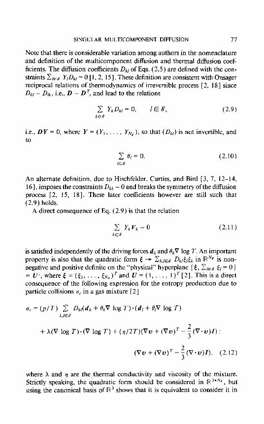
Note that there is considerable variation among authors in the nomenclature and definition of the multicomponent diffusion and thermal diffusion coefficients. The diffusion coefficients Dkl of Eqs. (2.5 ) are defined with the constraints Cl,s Y/D, = 0 [ 1,2, 151. These definition are consistent with Onsager reciprocal relations of thermodynamics of irreversible process [ 2, 181 since Dkl = Dlk, i.e., D = D’, and lead to the relations

c YkDkl = 0, 1E 8, (2.9) kE6

i.e., DY = 0, where Y = (Y,, . . . , Y,, ), so that ( Dkl) is not invertible, and to

c or = 0. (2.10) ES

An alternate definition, due to Hischfelder, Curtiss, and Bird [ 3, 7, 12- 14, 161, imposes the constraints Dkk = 0 and breaks the symmetry of the diffusion process [ 2, 15, 181. These later coefficients however are still such that (2.9) holds.

A direct consequence of Eq. (2.9) is that the relation

c Y, v, = 0 kE6

(2.11)

is satisfied independently of the driving forces dk and &V log T. An important property is also that the quadratic form [ + &JEB D&& in [RN’ iS nonnegative and positive definite on the “physical” hyperplane { [, C,,S &= 0 } = U’, where E = ([,, . . . , &v,)Tand U = (1, . . . , l)T [2]. This is a direct consequence of the following expression for the entropy production due to particle collisions uc in a gas mixture [ 21

UC = (p/T) 2 Dk,(dk + f&V log T). (d, + 6,V log T) k&8

+ X(V log T).(V log T) + (7/2T)(Vu + (VU)~ - ; (V.v)l) :

(Vu+(Vu)‘.-$V.u)I), (2.12)

where h and n are the thermal conductivity and viscosity of the mixture. Strictly speaking, the quadratic form should be considered in R 3*Ns, but using the canonical basis of R3 shows that it is equivalent to consider it in

78 VINCENT GIOVANGIC;LI

tR”#. Note also that D kl = 0( 1) for k # 1 whereas Dkk = O( I IX,) so that D~~-+ccwhenXk-+O[1,2].

2.2.2. Dual Multicomponent Di#iision Coeficients Ak,

It is also interesting to introduce the dual relations

dk + BkV log T = -C Ak,V/, IES

(2.13)

where A = ( Akl) is the dual multicomponent diffusion coefficient matrix. These coefficients are also symmetric, Akl = Ark, i.e., A = A’, and satisfy

1 A/c/ = 0, 1E 8, (2.14) kE8

i.e., AU = 0, so that the relation

2 dk=O kE8

(2.15)

is satisfied independently of the diffusion velocities vk. The quadratic f0I-m c + &/ES &,63;, in RN8 is also nonnegative and positive definite on the physical hyperplane { 5, C IES Y,& = 0 > = Y I, where r = ( cl, , <&and Y = (Y,, . . . . Y,, ) ‘. Note also that Akk = O(&) whereas Akj = 0(X,X,) for k # 1.

The relation between the matrices D and A can be clarified by using the theory of generalized inverses [ 191. Indeed, D and A are generalized inverses with prescribed range and null space. More specifically, A is the unique matrix with range U’ and nullspace lRlJ such that DAD = D and ADA = A and D is the unique matrix with range Y’ and nullspace [R Y such that ADA = A and DAD = D. From the theory of generalized inverses [ 191, one can show that AD and DA are projector matrices with range U’- and Y’ and nullspace [R Y and R U, respectively, which can be written

AD = Z - ( YU’)/( UTY), (2.16)

and

DA = I- (UYT)/(YrU). (2.17)

Only the former relation is well known and is usually written for one-term Sonine polynomial approximations and without the Y TU = ckE8 Yk term, although it is generally valid [l-3, 15, 161. Finally note that A is not the


Moore-Penrose pseudo-inverse [ 19, 201 D+ of D unless Y and U are proportional in which case DA and AD are orthogonal projectors.

A motivation for introducing the dual relations is that evaluating the multicomponent diffusion coefficients Dkl requires solving large linear systems, namely of size jlv, *ilv, when j terms are retained in the Sonine polynomial expansion of the species perturbed density probability functions [ 1, 21. This is not the case for the dual coefficients Ak, when j = 1, i.e., when only one term is retained in the latter expansion. Indeed, in this situation, the dual formulation reduces to the Stefan-Maxwell equations

xk& dk + BkV log T = 2 a, V,- vk, kE 8, (2.18) IE~ kl i#k Ifk

where a)k, denotes the usual binary diffusion coefficient for the species pair (k, 1). These relations, which must be completed by the mass constraint Eke8 Yk vk = 0 in order to define uniquely the diffusion velocities, may now be inverted to yield the diffusion velocities vk [ 1-4, 10, 14, 161.

Finally note that some care must be taken when applying the Onsager reciprocal relations to the entropy quadratic form C&G vk * dk since the fluxes vk, or the affinities dk, are constrained. One must indeed use the reciprocal relations for N8 - 1 fluxes or affinities and build the symmetric N6 * N8 diffusion matrices D and A from the corresponding ( N8 - 1) * ( NS - 1) symmetric positive definite matrices [ 3, 2 11. This procedure, of course, leads to matrices D and A which are nonnegative and positive definite on the proper hyperplanes.

2.2.3. Approximate D@ision Coejicients Dfl

Comparisons between different mathematical approximations of the multicomponent transport properties have shown that simplified transport expressions often provide a good trade-off between precision and computational costs [ 9, I2- 141. Hirschfelder and Curtiss [ 22 ] have first suggested the following expression for the diffusion velocity due to species gradients

0: = (1 - yk)/ 2 (x,/akl), IE8 I#k

(2.19)

where 0: is the diffusion coefficient of the kth species in the mixture. Note that this expression can be recovered from ( 2.16 ) and ( 2.18 ) by approximating A and D by their diagonal. However, the expressions (2.19) do not satisfy

80 VINCENT GIOVANG1C;I.I

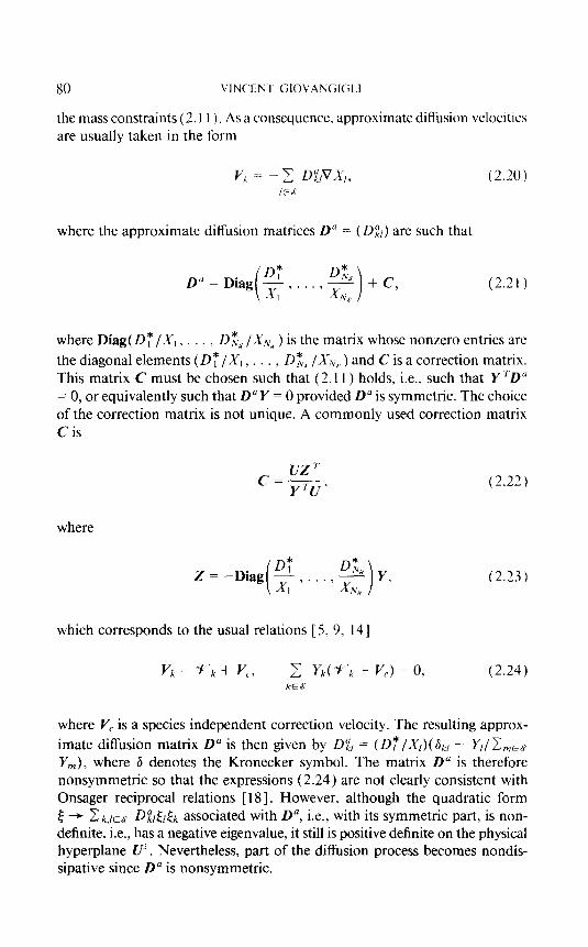
the mass constraints (2.1 1 ). As a consequence, approximate diffusion velocities are usually taken in the form

V, = - 2 D;l-,VX,, (2.20) /EA

where the approximate diffusion matrices D” = (D;I-1) are such that

(2.21)

where Diag(DT /Xl, . . , DE, /XAl.,> ) is the matrix whose nonzero entries are the diagonal elements (DT /XI, . . , D& /X,,), ) and C is a correction matrix. This matrix C must be chosen such that (2.11) holds, i.e., such that Y TD” = 0, or equivalently such that D”Y = 0 provided D” is symmetric. The choice of the correction matrix is not unique. A commonly used correction matrix C is

UZT C=----

YTU’

where

, (2.23)

(2.22)

which corresponds to the usual relations [ 5, 9, 141

c Yk( ̂ / ‘k + V,.) = 0, kGEP

(2.24)

where V, is a species independent correction velocity. The resulting approximate diffusion matrix D” is then given by Df, = (D?/X,)(& - Y,/ Cm,8 Y,), where 6 denotes the Kronecker symbol. The matrix D” is therefore nonsymmetric so that the expressions (2.24) are not clearly consistent with Onsager reciprocal relations [ 181. However, although the quadratic form 2: + 2 k,ES D$C;,.& associated with D”, i.e., with its symmetric part, is non- definite, i.e., has a negative eigenvalue, it still is positive definite on the physical hyperplane U’. Nevertheless, part of the diffusion process becomes nondis- sipative since Da is nonsymmetric.


2.3. Chemical Production Rates Wk and &

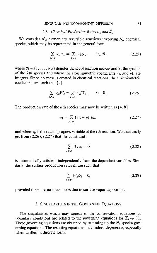
We consider NB elementary reversible reactions involving Na chemical species, which may be represented in the general form

2 VkiXk 5 2 U&xk, iE9?, (2.25) ke.8 ke8

whereB={l,... , NB } denotes the set of reaction indices and xk the symbol of the kth species and where the stoichiometric coefficients vii and u& are integers. Since no mass is created in chemical reactions, the stoichiometric coefficients are such that [ 41

c ukiwk = c viiwky iEYl. (2.26) kE8 kc3

The production rate of the kth species may now be written as [ 4, 8 ]

wk = 2 (v,& - v?ci)qi, iEi?

(2.27)

and where qi is the rate of progress variable of the ith reaction. We then easily get from (2.26), (2.27) that the constraint

(2.28)

is automatically satisfied, independently from the dependent variables. Sim- ilarly, the surface production rates i& are such that

c w,;j, = 0, ke8

(2.29)

provided there are no mass losses due to surface vapor deposition.

3. SINGULARITIESINTHEGOVERNING EQUATIONS

The singularities which may appear in the conservation equations or boundary conditions are related to the governing equations for C&8 Yk. These governing equations are obtained by summing up the Nd species governing equations. The resulting equations may indeed degenerate, especially when written in discrete form.


3.1. The Origin cf Singulurities

To investigate the singular behavior due to the mass constraints, we assume that a set of discrete equations modeling a multicomponent reacting mixture has been derived and we consider its Jacobian matrix formally written

n =

i

d(G”, G’, . . .) G‘v’b’, e*‘cy)

d(H, Y,, . . .1 y;,-I, Y,,) 1 ’ (3.1)

where H = (p, V, T) denotes the dependent variables aside from the species mass fraction, &H the corresponding discrete equations, and 6’ k the kth species discrete equations. The different dependent unknowns p, u, T, etc., are formally grouped into a single variable H and the dependence of discrete equations & on computational cells does not appear explicitly in (3.1) in order to avoid notational complexity. Furthermore, in this Jacobian matrix, the partial derivatives with respect to the mass fractions are assumed to be independent.

By adding now the lines corresponding to the equations G ‘, . . . , & N7-’ to the lines of 6 N*, at each computational cell, and substracting the columns corresponding to the derivation with respect to YNTV to the columns of Y,, . . . ) Yv#-r, at each computational cell, we get the following expression for the Jacobian d

d = det(lT) = det c3(GH, G’, . . . ) GN*-‘, &“)

d(H, Y,, . . . , Y,,-, , a) ’ (3.2)

where C = &&a Y, and G” = &,=S Gk. Note that in this new expression, the partial derivatives with respect to Yr , . . . , Y,,-, are taken with u = C&G Yk fixed. By regrouping then the lines corresponding to G” at the bottom of the later matrix in (3.2) and the columns corresponding to the partial derivatives with respect to (r on the right of this matrix, we obtain the block decomposition

d = det d(H, YI, . . . , y,,-I)

a(&“) \ d(H, YI, . . . , yN,-1)

On the other hand, for any physical solution, we have numerically CJ = c&S Yk = 1, and in this situation one may check from Eqs. (2.1)-( 2.29) that the lower left block in (3.3) is zero. We thus deduce that for any solution for which .&B Yk = 1 nUmeh.Xdly, we have the relation

d = l-T, (3.4)

SINGULAR MULTICOMPONENT DIF’FUSION 83

where

r = det d(&H, &‘, . . . ) cN”-‘) auf, yl) . . . , yN8-d ’

(3.5)

The determinant I? in ( 3.5) is the determinant that would be obtained by using YN8 = 1 - Ck+&. Y, in the governing equations. On the other hand, the determinant ‘I in ( 3.5 ) is simply that of the Jacobian matrix of the discrete system whose continuous equations and boundary conditions are obtained by summing all the corresponding species governing equations, and in which the unknown function is u = CkEB Yk. The singularities in the equations due to the mass constraints arise now when the later determinant r is zero.

These singularities may appear with any intermediate solution considered during iterative processes devoted to solve the discrete governing equations, like NeW.on’s method, for instance. These singularities may lead to convergence difficulties, or decrease the domain of convergence of various numerical methods or poor sensitivity information. Linear algebra solvers may also en- counter difficulties, especially those based on iterative techniques. They may also lead to artificial mass creation in such a way that u = 2~8 Yk is not uniformly unity so that the lower left block in (3.3) is no more zero. Different types of flow configurations may also lead to ‘I = 0 as detailed in the following where we investigate the governing equations for u = CLQ Yk.

3.2. Singularities for Steady Flows

By summing up the N8 equations (2.1) we get that

kE8

which specializes to

L’v*v( 2 yk) = 0, kE8

(3.6)

(3.7)

for steady flows. A direct consequence is that at a stagnation point where v = 0, Eq. (3.7) degenerates. In this situation, the Ns species equations, and thus the governing equations, are numerically linearly dependent, although the species are considered independent unknowns. Of course, this is still true when the Ns species equations are written in conservative form since then the sum of the species equations is proportional to the total mass equation at stagnation points. For similar reasons, it still holds if mole fractions or molar concentrations or number densities are used to describe the species.


From a discrete point of view, the Jacobian matrix II is then singular at grid points which exactly coincide with stagnation points. However, if u is small but nonzero, the Jacobian matrix II will still be ill conditioned. A typical example of steady flow involving a stagnation point is provided, for instance, by the flow obtained with two counterflowing jets [ 61. Any flow with recir- culation zones also involves stagnation points and thus leads to singular behavior.

Note also that when the simplified expressions (2.24) are used, the correction velocity V, must be evaluated from F’, = -( CkES Y@-k)/( CkEd, Yk). If V, is evaluated with the simplified expression V,. = -EkEa Ykv, [ 9, 11, 14]- which corresponds to the correction matrix C = UZ T instead of (2.22)- then CkEs Y, Vk does not sum up algebraically to 0 but to ( CkE8 Yk - 1 ) V, so that (3.7) is modified such that

(3.8)

which fortuitously may suppress the singularity at stagnation points. Nev- ertheless, if V. (pV,) = 0 and u + V, = 0 we still have singular behavior. Similarly, when V. V, and IJ + V, are small, the discrete equations are still ill conditioned. Our numerical experience indeed confirms that the term ( CkEB Yk - 1) ?‘, does not SatiSfaCtOdy stabilize the governing eqUatiOnS.

3.3. Singularities in Boundary Conditions

First, Dirichlet boundary conditions do not introduce any difficulty and provide that CkES Yk = 1 at that boundary. By summing up the NS species Neumann boundary conditions (2.3) we then get that

v( c Yk- 1)-n=& k&Y

(3.9)

which usually does not lead to singular discrete equations. However, a classical finite difference technique used to obtain centered second-order accurate, discrete boundary conditions consists in introducing ghost points, writing the centered discrete boundary conditions and governing equations at the boundary point and eliminating the ghost point values from the resulting set of equations. In one dimension, for instance, and for steady flows, the discrete Neumann boundary conditions for a nonreactive adiabatic wall lead to T,, = T-h and (Yk)h = (Yk)-h, where the subscripts h and -h refer to the first interior and ghost grid points respectively. Denoting Vk the nonzero compo- nent of the diffusion velocity vk = (vk, 0, 0), we deduce that (PYkVk)h/2 = - (p Y, Vk))h,~ where the mass diffusion fluxes are estimated with centered finite differences and where h/2 and -h/2 refer to the corresponding mid-


points. Using then the discrete equation (( pYkVk)h12 - (~YkVk)&)/h + (IV,&,, = 0, where we have used v = 0 and where the subscript 0 refers to the boundary point, we obtain the following species centered second-order accurate, Neumann discrete boundary condition and for one-dimensional steady flows

- ; (PYkvk/k)h,Z + (wkwk)O = 0, kE 8. (3.10)

These equations again lead to a singularity since generally the discrete flux velocities ( pYkVk),,, at h/2 algebraically sum up to zero. Here again, if the simplified expressions (2.24) are used with the incorrect formulation V, = -CkE8 Ykvk for V,, as in Eq. (3.8), then summing up the Ns species equations (3.10) leads to the boundary condition (( C.&B Yk - 1 )I’,),,, = 0, where V, = (I’,, 0, 0). In this situation, the nonsingular behavior relies on the poorly known term I’,, and our numerical experience confirms that this term does not satisfactorily stabilize the centered boundary conditions ( 3.10).

Finally, by summing up the Ns species mixed boundary conditions (2.4) we get that

p,,-,t( 2 Yk- 1) = 0, kE8

(3.11)

so that when u * n = 0 the equation degenerates for both steady and unsteady flows. Note that a typical situation where u * n = 0 and pYk vk. n = w&k is, for instance, that of a solid-gas interface with no surface vapor deposition. On the other hand, for a plane laminar flame, we have m = pu = pv * n # 0, where m is the laminar flame eigenvalue which is positive [ 1 l] and there is no singularity.

We also note here that besides considering p, Y, , . . . , Y,, , v, and T as the dependent variables, as in our analysis, or p, Y, , . . . , Y,,-, , v, and T, when- ever there is an excess species, it is sometimes proposed to consider pi, . . . , pNs, V, and T, where the Pk = pYk are the species densities. In this situation, the mixture density is evaluated from p = C&G Pk and the total mass conservation equation is discarded. However, this formulation does not suppress the singularities arising from boundary conditions. Moreover, it is usually desirable to distinguish between the total mass conservation equation and the species mass conservation equations since the former is first order whereas the later are second order and may, for instance, be discretized differently.

4. MODIFIEDDIFFWONALGORITHMS

In this section we modify the various diffusion algorithms in order to eliminate the singularities exhibited in the previous section. These singularities


are indeed due to the absence of suitable diffusion terms in the various governing equations for CkES Yk. Diffusion terms are indeed missing because diffusion matrices are not invertible due to the mass conservation constraints. In order to locate the origin of the problems, it is very instructive to assume for a while that dk + 0kV log T = VXk. In this situation the numerical difficulties are due to the singular diffusion matrix A4 such that pYk P”A = -CIEs MkrVYJ, which may be written M = pDiag(Y,, . . . Y,v, ) DE. where Diag(Y,, . . . , Y,vX) is the matrix whose nonzero entries are the diagonal elements (Y, , . . . , YvZ ), D the diffusion matrix of Eq. (2.5 ), and E = (Elm) = ((W/W)(61, - ~W/W,)) is such that

VX, = c E,,,,VY,. (4.1) rnE8

But the matrix M is not invertible since, first, D is not invertible and, second, i5’fs yt invertible, because CkES & = 1 implies that CkEs V& = 0 and

kEB Ek, = 0. Therefore we deduce from this simple analysis that part of the difficulties are due to the matrix E, i.e., to the relations between mole and mass fractions, and part are due to the matrix D, i.e., to the diffusion algorithms.

4.1. Mole and Mass Fractions

The matrix E, which relates the gradients of the mole fractions to those of the mass fractions, is singular because Eq. (2.8) imposes the relation Cktd & = 1 independently of the mass fractions. Similarly, the dual relations between X, and Y, [ 4, 81, usually expressed with (2.7) and

w= c xkwk, kES

(4.2)

lead to the relation C&S Yk = 1 independently of the mole fractions so that the matrix F, which relates the gradients of the mass fractions to these of the mole fractions.

VYI = C F,mV-Kn, (4.3) rnE8

is also singular. In both cases, the singularity of E and F is due to the fact that the corresponding constraints C&S & = 1 and C&S Yk = 1 are imposed a priori.

The correct formulation for W is indeed

( 2 yk)/w = 2 yk/ wk, kE8 kE6

(4.4)


since it leads to invertible relations between & and Y, and provides the identity

c xk = 2 yk. kE8 kE8

(4.5)

The dual formulation, which now can be deduced from (2.7) and (4.4), is then

( c xk)w= c xkwk. (4.6) kES kES

With these new relations the matrices E and F become invertible and are inverse of each other and one may easily check that det( E) = n&S (W/ wk) . Finally, from the relations (2.6), (2. lo), and (4.5 ) we get the important relation

c (dk + ekv log T) = c vxk = v( 2 xk) = v( 2 Yk), (4.7) kES kE6 kE8 X-ES

since the thermal diffusion, pressure, and external force terms algebraically sum up to zero.

4.2. Difusion Velocities

As for the matrices E and F, the singularity of the matrices D and A is due to the fact that the corresponding mass constraints (2.11) and (2.15) are imposed a priori. Now any modification of the diffusion matrix D should take into account the symmetry of D, leave unchanged the physical hyperplane {E, Cm b=O) = U’, and promote the positivity of D. We must thus modify D in the form

B=DD&JUT, (4.8)

where d denotes the modified matrix, U the vector U = ( 1, . . . , 1)) and CY a positive function. Note that the resulting matrix d is positive definite since D is positive on U”- and (Y UU T is positive on IR U. The corresponding diffusion velocities satisfy now

c Yk vk = -a 2 (dk i- &v log T), kE8 kE8

(4.9)

where 2 = cr( CkE8 Yk) is positive, which combined with (4.7) yields the important relation

x Ykv, = -a)v( 2 Yk). kES kE8

(4.10)


Further note that the matrix pDiag( Y, , . . Y,v”, )d relating the mass fluxes pYk Vk to the mole fraction gradients VX,, which is not symmetric, has bounded coefficients and has positive eigenvalues as product of two positive definite symmetric matrices [ 20, 231.

The dual relations must also be modified into

A=A++YY’. (4.11)

where 6 denotes the modified matrix, Y the vector Y = ( Y, , . . , YNq ), and ,6 a positive function. The resulting matrix 6 is positive definite since A is positive on Y’ and PYY r is positive on tR Y. One may easily check that when (Y and /3 are related through the relation

4% c yk)* = 1, k E 8

(4.12)

where UTY = Y ‘ZJ = C b w

ktS Y,, we then have AD = I, where Z is the identity matrix. The modified matrices 6 and d are thus inverses of each other whereas A and D are only generalized inverses of each other. Note that the relation Ad = Z may be a convenient way to evaluate D from A, using either direct or iterative techniques.

A consequence of (4.11) is that the following modified Stefan-Maxwell equations,

dk + 0kV log T = C xkxl - -

/ES akl I+k

kE cc?, (4.13)

IZk

define uniquely the diffusion velocities vk and automatically handle mass conservation constraints in the sense that

-o( z yk) 2 ykvk = 2 (6 + ekv 1% n. kE8 kES kES

(4.14)

To our knowledge, the modified expressions (4.8 ), (4. lo), (4.11)) and (4.13 ) have not previously been written although related ideas may be found in the literature. For instance, ( NS + 1) * ( NS + 1) regular diffusion matrices


are considered in Chapman and Cowling [ 11. These matrices, however, un- necessarily increase the size of the linear systems. Linearly independent diffusion driving forces dk are also considered in Ferziger and Kaper for different purposes [ 2 1.

Similarly, the simplified expressions (2.24) must now be completed with

c Yk(Vk + Vc) = -3V( c Yk), kc8 kES

(4.15)

which corresponds to the modified approximated diffusion matrix da = D” + aUUT. The associated quadratic form can be shown to be positive definite for a> = a( C&,.$ Yk) large enough. Moreover, since D” is not symmetric, one may also introduce nonsymmetric modifications such that da = Da + RUT, where R is a somewhat arbitrary vector. Jones and Boris have indeed introduced an 0( Ni ) iterative algorithm [ 10, 17 ] to invert the Stefan-Maxwell equations (2.16) based on the simplified expressions (2.24) and these authors pointed out that using modified matrices like da = D” + RUT, where R is arbitrary, was feasible. However, they have found it convenient to use R = 0 [lo].

4.3. Nonsingular Behavior

We must now investigate the properties of the governing equations when the modified relations (4.8)) (4.11)) and (4.15 ) are used. Summing up the N8 species equations (2.1) for a steady flow, we first get from (4.10) that

Pvev( c yk) = -v(av( c yk))> (4.16) kE8 kES

and the new artificial diffusion term suppresses the singular behavior at stagnation points. Heuristically, C&B Yk behaves now like a new species which tends to diffuse until the equilibrium state CkES Yk = 1, normally imposed by the boundary conditions, is reached. But once the equilibrium state is reached, we then have C&S & = 1 from (4.5) and C&S Yk vk = 0 from ( 4.10) so that ultimately the mass constraints are numerically satisfied. Note that the origins of small deviations of C kE$ Yk from Unity are the iterative processes devoted to solve the discrete governing equations like, for instance, Newton’s method [ 1 I]. Note also that the extra diffusion term V * (XIV ( CkEB Yk)) stabilizes the equations more satisfactorily than the term involved in Eq. (3.8).

By summing up the Ns species centered second-order accurate, Neumann discrete boundary condition ( 3.10) for one-dimensional steady flows, we also get


(PV( c Yk))h,7 = 0. XEI

(4.17)

which suppresses the singular behavior observed with (3. IO). Similarly, for the boundary conditions (2.4) when us n = 0, we now get.

by summing up the NS species equations, that

V( c Y,). n = 0, k E S

(4.18)

which again suppresses the artificial singular behavior. The species C&S YL of course appears as nonreactive in (4.18 ) .

More generally, the boundary value problem in 0 = C&S Yk obtained by summing up all the species equations and boundary conditions-whose Ja- cobian matrix has determinant r-is a linear convection-diffusion problem which is generally well posed. Of course, by modifying the mole/mass fractions relations and the diffusion matrices, we have only suppressed the artificial singularities due to the mass constraints which arise through the r term in (3.4). Other types of singularities, like those which appear at extinction limits. i.e., simple turning points, may still occur [ 61 and arise through the r term in (3.4). Furthermore, suppressing the artificial singularities due to the mass conservation constraints does not eliminate other numerical problems which may arise in (2.5), (2.18), or (2.24) like, for instance, those of vanishing small concentrations [ 7, 91.

5. NUMERICALEXPERIMENTS

5 _ 1. Singular Value Decompositions

Our first numerical investigations are concerned with the matrices A from the Stefan-Maxwell equations (2.18 )

Akk = c z > IES I#k

xkxl &, = - -

akl ’ k# 1. (5.1)

We have performed singular value decompositions of the matrix A for various mixtures, including a 9 species mixture used for hydrogen-air flames [ 61 and a 16 species mixture used for methane-air flames [ 6 1, under various tem-


perature and pressure conditions. The binary coefficients a)k, have been taken in the form

(5.2)

where &l is the reduced mass of the species pair (k, 1)) dk[ is the collision diameter of the species pair (k, I) and tl(‘,‘)* is a reduced collision integral. The reduced collision integral Q (L’)* depends on the reduced temperature Tz, = k,T/tkl, where tk/ is the Lennard-Jones potential well depth of the species pair (k, I) and on various other molecular parameters. The species pair mOleCUlar parameters tk[, (Tk[, etc., have been evaluated according to the Usual IktUre rule fOrmUlas, e.g., Ukl = ( (Tk + al)/2 and tkl = I&. We refer to [ 71 for more details. In our numerical tests, we have always found only one zero eigenvalue and N8 - 1 positive eigenvalues, in agreement with the kinetic theory of gases and Onsager relations. Note also that from ( 5.1) and the Gerschgorine theorem [ 23,241, all the eigenvalues of A are nonnegative.

We have then performed singular value decompositions for the corresponding modified diffusion matrices A = A + p Y Y r with a value of p = 1. We have obtained only positive eigenvalues for the modified matrices 6. A typical result is presented in Table I for an equimolar mixture, i.e., & = 1 / N8, consisting of the N8 = 9 species HZ, 02, H20, NZ, OH, HO*, H202, H, and 0 at temperature T = 1000 IS and p = 1 atm. Note that the eigenvalue of A and 6 are nested, according to a classical result of linear algebra [20, 231.

5.2. Determinant Evaluations

In order to inve,stigate numerically the nonsingular behavior of the modified equations in a practical situation, we have computed premixed symmetric hydrogen-air flame structures. For such flames, the governing equations can be written in the form [ 61

TABLE I EIGENVALUES (* 100) OF A AND 6 FOR AN EQUIMOLAR MIXTURE OF THE

Ns = 9 SPECIES Hz, 02, H20, NZ, OH, HOz, Hz02, H, AND 0

1 2 3 4 5 6 I 8 9

A 0.00 0.916 1.52 3.20 3.45 4.04 4.88 4.91 4.92 6 0.809 1.35 3.19 3.31 3.81 4.88 4.90 4.91 15.70

92 VINCENT GIOVANGIC;LI

- t( pj - pz.2’) = 0, (5.4)

dYk d pu - + - (PYkVk) - w,w, = 0,

dy dy k = 1, . . . ) N$, (5.5)

+(; pYkVkcpk)$+ ;: hkWkwk=O, (5.6) k=l k=l

where y denotes the spatial coordinate normal to the stagnation plane; p, the mass density; u, the velocity in the normal direction (y); t, the strain rate; 6, a similarity function related to the velocity u in the transverse direction (x) so that u = (txu”, V, 0); TJ, the mixture viscosity; ,of, the mass density in the fresh reactant stream; Yk, the mass fraction of the kth species; Ns, the number of species; V,, the diffusion velocity of the kth species in the normal direction, so that vk = (0, vk, 0); W,, the molecular weight of the kth species; wk, the molar rate of production ofthe kth species; T, the temperature; X, the thermal conductivity of the mixture; c,, the constant pressure heat capacity of the mixture; cpk, the constant pressure heat capacity of the kth species; and hk, the specific enthalpy of the kth species. Complete specification of the problem requires that boundary conditions be imposed at each end of the computational domain. As y --* +co we have

lz= 1, yk = ykf,

and for y = 0 we have

2, = 0, du LIZ 0, dyk

dv

- zz 0,

&

k= 1,.

k= I . , Ns

T= Tf, (5.7)

dT - = 0, (5.8) dv

where T/is the specified temperature in the fresh reactant stream and Ykfthe specified mass fractions in the fresh reactant stream. These equations have also to be completed by formulas expressing the transport coefficients h and 7, the diffusion velocities vk, the thermodynamic properties c,, c&, and hk, and the chemical production rates wk. More details on the modeling can be found in [4-6, 8, 91.


The steady equations ( 5.3)-( 5.8 ) have been discretized with finite differences and solved using Newton’s method and adaptive gridding techniques [ 6, 111. A reference solution corresponding to a fresh mixture of 8.5% of hydrogen in mole and a strain rate of e = 50 s-’ has been obtained. From Eqs. ( 5.5 ) we note that, for our test problem, it is the normal velocity II which determines the singular behavior in the species mass conservation equations. But in this flow configuration the velocity v is negative on (0, + cc ) , so that there are no singularities with Eqs. ( 5.5). Moreover the Neumann boundary conditions (5.8) at y = 0 have been discretized with first-order schemes, thus avoiding the singularities introduced with (3.10).

We then have perturbed the reference solution in order to introduce singularities and we have computed the corresponding Jacobians. The calculations have been performed with the one-dimensional simplified transport expressions (2.24) using either the exact correction velocity V,, obtained from (2.24)

vc, = -( c yk-trk)/( 2 yk), kES kES

where

v= D:dxk k

xk dy ’

or the often used simplified expression VcI

vc2 = - c ykvk, kES

(5.9)

(5.10)

(5.11)

or the modified expression Vc3 obtained from (4.15 )

vc3=- c y,y.,+akzS$ (2 yk), (5.12) kES keS

with a value of CY = 1. Calculations have been done in double precision, i.e., with 64-bit words, and Jacobian matrices have been evaluated numerically by finite differences so that their accuracy is only simple precision. Denoting X the discrete reference solution, obtained on a mesh 0 = y. < y1 < * - - , and V, the normal velocity at node yj, we have considered the perturbed discrete vectors Xj, j > 1, obtained by setting vl = * - - = Vj = 0 in x,


TABLE II DECIMAL L~CARITHMSOFREDUCEDJACOBIAN SINGULARITIES

INTHESPECIESCONSERVATION EQUATIONS

Vd -I 1.84 -21.43 -33.66

Vf v : -3.72 -0.01 m-7.43 -0.03 -11.12 PO.07

respectively. Note that o. = 0 in X so that X, is very close to X when j is small. We have then evaluated the Jacobians (3.1) d and ~9, at X and X,, respectively. The decimal logarithms of the ratios dj/b are presented in Table II forj = 1, 2, 3, in columns X,/X, j = 1, 2, 3, respectively, as a measure of the singularities introduced by stagnation points for the different correction velocities I’,, , V,, and I’,,.

We note that with the formulation I’,, more than 10 orders of magnitude are lost at each new zero velocity Vj. In this situation the code was unable to converge back from XI to 5%. On the other hand, the corresponding Jacobians evaluated with the expression VCj are almost unperturbed by the zero velocities, and the code was able to converge back immediately from XI, X2, or X3 to 5%. With the simplified expressions VC2, we note that only 3 orders of magnitude are lost at each new zero velocity. This is due to the right hand side term in Eq. (3.10). However, this term can be seen to lead to singularities when VC1 vanishes in the neighborhood of the origin. As a consequence we have also considered the perturbed discrete vectors X,* , j = 1, 2, 3, obtained from X,) j = 1, 2, 3, by flattening the temperature and species profiles near the origin, i.e., by setting To = T, = T2 = T3 = T4 and Y, = Y,, = Y,, = Y,, = Yk4, k = 1 . . 9 Na. Note that with our value of the strain rate t = 50 SC’ and from Neumann’s boundary conditions (5.8) the perturbed discrete vectors XT, j = I, 2, 3, are very close to 5%. Starting now from XT, the code was not able to converge back to X, and the convergence from X 7 and 5%; was maintained only by using a very efficient damping strategy in Newton’s method [ 11, 241 together with a very small damping parameters. On the other hand, with the expressions VC3, Newton’s method converges back immediately from X T to x.

Finally, using the reference solution X, we have investigated the singular behavior in boundary conditions by using the discrete equations

bYkVk)h/2 = 0, (5.13)


TABLE III DECIMAL LOGARITHMS OF REDUCED JACOBIAN SINGULARITIES

IN THE BOUNDARY CONDITIONS

X

Vd I vc3 -9.33 vcz I vc3 -16.32

instead of the usual first-order Neumann boundary conditions. These equations lead to the same type of singularities as the centered boundary conditions ( 3.10). For the different expressions V,r , I’, , and V,, we have evaluated the corresponding Jacobians denoted by d,r , dc2, and dc3. The decimal logarithms of the ratios 6,, / dc3 and a,/ dc3 are presented in Table III as a measure of the singularities introduced by boundary conditions, at the lines I’,, /V,, and L’, / V,, , respectively. This table shows that 10 orders of magnitude are lost with the singularity introduced by V,, whereas 16 orders of magnitude are lost with I’,, . Finally, it is also interesting to note that, depending on initial estimates, spurious converged solutions involving artificial mass creation have been observed with both expressions I’,, and I’, . More specifically, denoting aj the sum CkEB Yk at node yj, some of the converged solutions have been found to be such that u. # 1 whereas ul = 62 = - . * = 1. Of course, this was never observed with V,, .

6. CONCLUSION

We have investigated mass conservation in multicomponent diffusion algorithms. Various singularities in the governing equations, due to mass conservation constraints, have been exhibited when all mass fractions are considered independent unknowns. Modifications of the usual diffusion algorithms have been introduced to eliminate these artificial singularities. Consistent modifications are proposed for three different diffusion algorithms, namely for the complex formalism of the kinetic theory of gases, for the Stefan-Maxwell equations, and for the Hirschfelder-Curtiss expressions with mass correctors. These modifications, of course, do not change the actual values of the diffusion velocities. Only their mathematical expressions are changed. Finally, we have tested the modified expressions by computing various flame structures and we have found that they improve both the accuracy and the robustness of our numerical algorithms.


ACKNOWLEDGMENTS

I thank Dr. B. Laboudigue and Dr. L. Sainsaulieu for interesting discussions concerning this material.

REFERENCES

I. S. Chapman and T. G. Cowling, The Mathematical Theory ofNon-Unlniforrn Gases. Cambridge Univ. Press, Cambridge ( 1970 )

2. J. H. Ferziger and H. G. Kaper, Mathematical Theory qf Transport Processes in G’asrc. North-Holland, Amsterdam ( 1972 ).

3. J. 0. Hitschfelder, C. F. Curtiss, and R. B. Bird, Molecular Theory ofGases and Liquids Wiley, New York (1954).

4. F. A. Williams, Combustion Theory, 2nd ed. Benjamin/Cummings, Menlo Park, CA ( 1985). 5. V. Giovangigli and N. Darabiha, Vector computers and complex chemistry combustion. In

C. Brauner and C. Schmidt-Laine (Eds.), Proc. Conference Mathematical Modeling in Com- bustion and Related Topics, NATO AS1 Series, Vol. 140, pp. 491-503. Nijhoff, The Hague (1988).

6. V. Giovangigh and M. D. Smooke, Adaptive continuation algorithms with application to combustion problems. Appl. Numer. Math. 5, 305-33 1 ( 1989).

7. R. J. Kee, G. Dixon-Lewis, J. Warnatz, M. E. Colttin, and J. A. Miller, A Fortran computer code package for the evaluation of gas-phase multicomponent transport properties. SANDIA National Laboratories Report, SAND86-8246 ( 1986).

8. R. J. Kee, J. A. Miller, and T. H. Jefferson, CHEMKIN: A General-purpose, problem-independent, transportable, Fortran chemical kinetics code package. SANDIA National Lab- oratories Report, SANDEO-8003 ( 1980).

9. R. J. Kee, J. Wamatz, and J. A. Miller, A Fortran computer code package for the evaluation of gas-phase viscosities, conductivities, and diffusion coefficients. SANDIA National Labo- ratories Report, SAND83-8209 ( 1983).

10. E. S. Oran and J. P. Boris, Detailed modeling of combustion systems. Progr. Energy Combust Sci. 7, l-72 (1981).

11. M. D. Smooke, Solution of burner-stabilized premixed laminar flames by boundary value methods. J. Comput. Phys. 48, 72-105 ( 1982).

12. J. Warnatz, Calculation of the structure of laminar flat flames, I. Flame velocity of freely propagating ozone decomposition flames. Ber. Bunsenges. Phys. Chem. 82, 193-200 ( 1978 ).

13. J. Wamatz, Influence of transport models and boundary conditions on flame structure. In N. Peters and J. Warnatz (Eds.), Numerical Methods in Laminar Flame Propagation, pp. 87- 11 I. Vieweg Verlag, Braunschweig ( 1982).

14. T. P. Coffee and J. M. Heimerl, Transport algorithms for premixed. Laminar steady-state flames. Combust. Flame 43, 273-289 ( 198 1).

15. C. F. Curtiss, Symmetric gaseous diffusion coefficients, J. Chem. Phys. 49,29 17-29 19 ( I968 ) 16. G. Dixon-Lewis, Flame structure and flame reaction kinetics. II. Transport phenomena in

multicomponent systems. Proc. Roy. Sot. A 307, 1 1 1-l 35 ( 1968).


17. W. W. Jones and J. P. Boris, An algorithm for multispecies diffusion fluxes. Comput. Chem. 5, 139-146 (1981).

18. J. Van de Ree, On the definition of the diffusion coefficients in reacting gases. Physicu 36, 118-126 (1967).

19. A. Ben-Israel and T. N. E. Grenville, Generalized Inverses, Theory and Applications. Wiley, New York (1974).

20. G. H. Golub and C. F. Van Loan, h4atrix Computations. Johns Hopkins Univ. Press, Baltimore (1983).

2 1. L. C. Woods, The Thermodynamics of Fluid Systems, Oxford Engineering Science Series, Vol. 2. Clarendon press, Oxford ( 1986).

22. J. 0. Hirschfelder and C. F. Curtiss, Flame propagation in explosive gas mixtures. In Third Symposium (International) on Combustion, pp. 121-127. Reinhold, New York ( 1949).

23. J. H. Wilkinson, The Algebraic Eigenvalue Problem. Clarendon Press, Oxford ( 1965).

24. P. Deuflhard, A modified Newton method for the solution of ill-conditioned systems of nonlinear equations with application to multiple shooting. Numer. Math. 22,289-3 15 ( 1974).

mass conservation and singular multicomponent diffusion

Documents