math 2280-001 week 13 april 10-14

> >

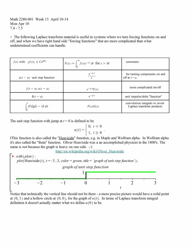
Math 2280-001 Week 13 April 10-14Mon Apr 107.4 - 7.5

The following Laplace transform material is useful in systems where we turn forcing functions on and off, and when we have right hand side "forcing functions" that are more complicated than what undetermined coefficients can handle.

f t with f t CeM t F s0

f t e s t dt for s M comments

u t a unit step function

e a s

s for turning components on and off at t = a .

f t a u t a e a sF s more complicated on/off

t a e a s unit impulse/delta "function"

0

tf g t d F s G s

convolution integrals to invert Laplace transform products

The unit step function with jump at t = 0 is defined to be

u t = 0, t 0

1, t 0 .

IThis function is also called the "Heaviside" function, e.g. in Maple and Wolfram alpha. In Wolfram alphait's also called the "theta" function. Oliver Heaviside was a an accomplished physicist in the 1800's. The name is not because the graph is heavy on one side. :-)

http://en.wikipedia.org/wiki/Oliver_Heavisidewith plots : plot Heaviside t , t = 3 ..3, color = green, title = `graph of unit step function` ;

t3 2 1 0 1 2 3

1graph of unit step function

Notice that technically the vertical line should not be there - a more precise picture would have a solid pointat 0, 1 and a hollow circle at 0, 0 , for the graph of u t . In terms of Laplace transform integral definition it doesn't actually matter what we define u 0 to be.

Then

u t a = 0, t a 0; i.e. t a

1, t a 0; i.e. t a

and has graph that is a horizontal translation by a to the right, of the original graph, e.g. for a = 2:

Exercise 1) Verify the table entries

u t a unit step function

e a s

s for turning components on and off at t = a .

f t a u t a e a sF s more complicated on/off

Exercise 2) Consider the function f t which is zero for t 4 and with the following graph. Use linearity and the unit step function entry to compute the Laplace transform F s . This should remind you of a homework problem from the assignment due tomorrow - although you're asked to find the Laplace transform of that step function directly from the definition. In your next week's homework assignment you will re-do that problem using unit step functions. (Of course, you could also check your answer in this week's homework with this method.)

t0 1 2 3 4 5 6 7 8

0

1

2

Exercise 3a) Explain why the description above leads to the differential equation initial value problem for x t

x t x t = .2 cos t 1 u t 10 x 0 = 0 x 0 = 0

3b) Find x t . Show that after the parent stops pushing, the child is oscillating with an amplitude of exactly meters (in our linearized model).

> >

Pictures for the swing:

plot1 plot .1 t sin t , t = 0 ..10 Pi, color = black : plot2 plot Pi sin t , t = 10 Pi ..20 Pi, color = black : plot3 plot Pi, t = 10 Pi ..20 Pi, color = black, linestyle = 2 : plot4 plot Pi, t = 10 Pi ..20 Pi, color = black, linestyle = 2 : plot5 plot .1 t, t = 0 ..10 Pi, color = black, linestyle = 2 : plot6 plot .1 t, t = 0 ..10 Pi, color = black, linestyle = 2 : display plot1, plot2, plot3, plot4, plot5, plot6 , title = `adventures at the swingset` ;

t2 4 6 8 12 16 20

3113

adventures at the swingset

Alternate approach via Chapter 3:

step 1) solvex t x t = .2 cos t

x 0 = 0 x 0 = 0

for 0 t 10 .

step 2) Then solvey t y t = 0y 0 = x 10

y 0 = x 10 and set x t = y t 10 for t 10 .

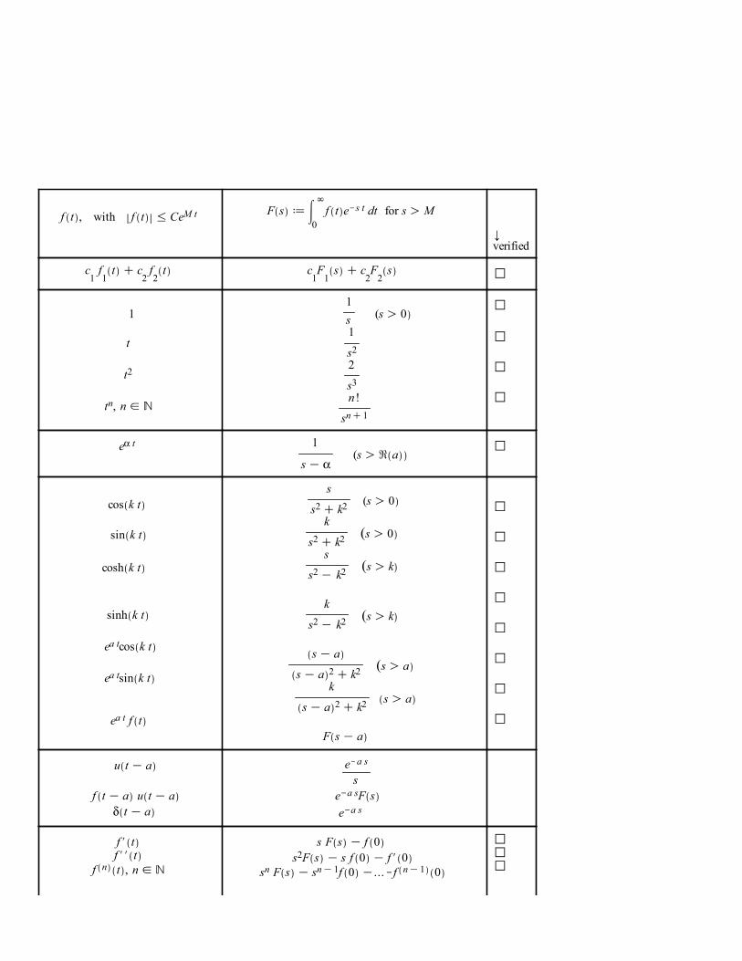
Laplace transform tableLaplace transform table

f t , with f t CeM t F s

0f t e s t dt for s M

verified

c1 f

1t c

2 f2

t c1F

1s c

2F

2s

1

t

t2

tn, n

1s (s 0 1

s2

2

s3

n !

sn 1

e t 1

s (s a

cos k t

sin k t

cosh k t

sinh k t

ea tcos k t

ea tsin k t

ea t f t

s

s2 k2 (s 0

k

s2 k2 (s 0

s

s2 k2 (s k

k

s2 k2 (s k

s a

s a 2 k2 (s a

k

s a 2 k2 s a

F s a

u t a

f t a u t a t a

e a s

s e a sF s

e a s

f t f t

f n t , n

s F s f 0 s2F s s f 0 f 0

sn F s sn 1f 0 ... f n 1 0

Laplace transform tableLaplace transform table

0

tf d F s

s

t f t t2 f t

tn f t , n f t

t

F s F s

1 n F n s

sF d

t cos k t

12 k t sin k t

1

2 k3 sin k t k t cos k t

t ea t

tn e a t, n

s2 k2

s2 k2 2

s

s2 k2 2

1

s2 k2 2

1

s a 2n !

s a n 1

0

tf g t d F s G s

f t with period p

1

1 e ps0

p

f t e s t dt

EP 7.6 impulse functions and the operator.

Consider a force f t acting on an object for only on a very short time interval a t a , for example as when a bat hits a ball. This impulse p of the force is defined to be the integral

pa

af t dt

and it measures the net change in momentum of the object since by Newton's second lawm v t = f t

a

am v t dt =

a

af t dt = p

m v tt = a

a= p .

Since the impulse p only depends on the integral of f t , and since the exact form of f is unlikely to be known in any case, the easiest model is to replace f with a constant force having the same total impulse, i.e.to set

f = p da,

t where d

a,t is the unit impulse function given by

da,

t =

0, t a1

, a t a

0, t a

.

Notice that

a

a

da,

t dt =a

a 1 dt = 1 .

Here's a graph of d2, .1 t , for example:

t0 1 2 3 4

0

610

Since the unit impulse function is a linear combination of unit step functions, we could solve differential equations with impulse functions so-constructed. As far as Laplace transform goes, it's even easier to take the limit as 0 for the Laplace transforms d

a,t s , and this effectively models impulses on very

short time scales.

da,

t =1

u t a u t a

da,

t s =1 e a s

se a s

s

= e a s 1 e s

s .

In Laplace land we can use L'Hopital's rule (in the variable ) to take the limit as 0:

lim0 e a s 1 e s

s= e a s lim

0

s e s

s= e a s.

The result in time t space is not really a function but we call it the "delta function" t a anyways, and visualize it as a function that is zero everywhere except at t = a, and that it is infinite at t = a in such a way that its integral over any open interval containing a equals one. As explained in EP7.6, the delta "function"can be thought of in a rigorous way as a linear transformation, not as a function. It can also be thought of as the derivative of the unit step function u t a , and this is consistent with the Laplace table entries for derivatives of functions. In any case, this leads to the very useful Laplace transform table entry

t a unit impulse function e a s for impulse forcing

> >

> >

> >

> >

> >

> >

Exercise 4) Revisit the swing. In this case the parent is providing an impulse each time the child passes through equilibrium position after completing a cycle.

x t x t = .2 t t 2 t 4 t 6 t 8 x 0 = 0

x 0 = 0 .

with plots :plot1 plot .1 t sin t , t = 0 ..10 Pi, color = black : plot2 plot Pi sin t , t = 10 Pi ..20 Pi, color = black : plot3 plot Pi, t = 10 Pi ..20 Pi, color = black, linestyle = 2 : plot4 plot Pi, t = 10 Pi ..20 Pi, color = black, linestyle = 2 : plot5 plot .1 t, t = 0 ..10 Pi, color = black, linestyle = 2 : plot6 plot .1 t, t = 0 ..10 Pi, color = black, linestyle = 2 : display plot1, plot2, plot3, plot4, plot5, plot6 , title = `Wednesday adventures at the swingset` ;

t2 4 6 8 10 12 14 16 18 20

3113

Wednesday adventures at the swingset

impulse solution: five equal impulses to get same final amplitude of meters - Exercise 1:f t .2 Pi sum Heaviside t k 2 Pi sin t k 2 Pi , k = 0 ..4 :plot f t , t = 0 ..20 Pi, color = black, title = `lazy parent on Friday` ;

t2 4 6 8 10 14 20 3

03

lazy parent on Friday

Or, an impulse at t = 0 and another one at t = 10 .

> > > >

> >

g t .2 Pi 2 sin t 3 Heaviside t 10 Pi sin t 10 Pi :plot g t , t = 0 ..20 Pi, color = black, title = `very lazy parent` ;

t2 4 6 8 10 14 20

3113

very lazy parent

> >

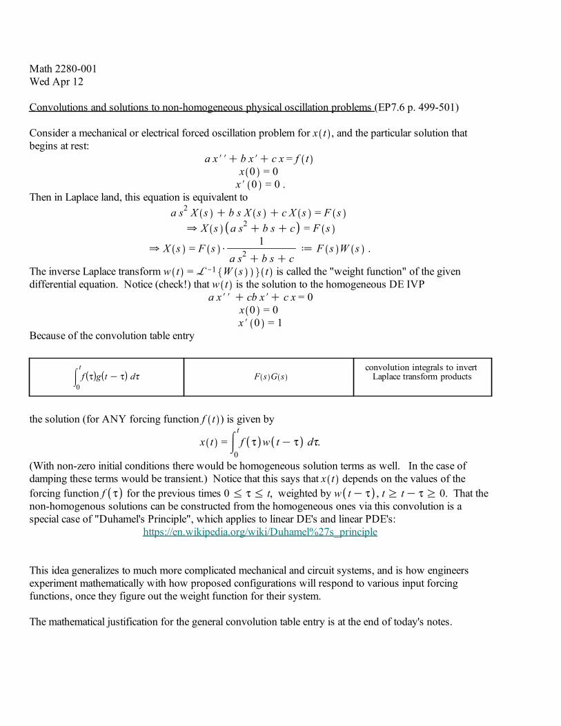
Math 2280-001Wed Apr 12

Convolutions and solutions to non-homogeneous physical oscillation problems (EP7.6 p. 499-501)

Consider a mechanical or electrical forced oscillation problem for x t , and the particular solution that begins at rest:

a x b x c x = f t x 0 = 0

x 0 = 0 .Then in Laplace land, this equation is equivalent to

a s2 X s b s X s c X s = F s X s a s2 b s c = F s

X s = F s1

a s2 b s cF s W s .

The inverse Laplace transform w t = 1 W s t is called the "weight function" of the given differential equation. Notice (check!) that w t is the solution to the homogeneous DE IVP

a x cb x c x = 0x 0 = 0 x 0 = 1

Because of the convolution table entry

0

tf g t d F s G s

convolution integrals to invert Laplace transform products

the solution (for ANY forcing function f t ) is given by

x t =0

tf w t d .

(With non-zero initial conditions there would be homogeneous solution terms as well. In the case of damping these terms would be transient.) Notice that this says that x t depends on the values of the forcing function f for the previous times 0 t, weighted by w t , t t 0. That the non-homogenous solutions can be constructed from the homogeneous ones via this convolution is a special case of "Duhamel's Principle", which applies to linear DE's and linear PDE's:

https://en.wikipedia.org/wiki/Duhamel%27s_principle

This idea generalizes to much more complicated mechanical and circuit systems, and is how engineers experiment mathematically with how proposed configurations will respond to various input forcing functions, once they figure out the weight function for their system.

The mathematical justification for the general convolution table entry is at the end of today's notes.

(1)(1)

> >

> >

> >

Exercise 2. Let's play the resonance game and practice convolution integrals, first with an old friend, but then with non-sinusoidal forcing functions. We'll stick with our earlier swing, but consider various forcing periodic functions f t .

x t x t = f t x 0 = 0 x 0 = 0

a) Find the weight function w t .b) Write down the solution formula for x t as a convolution integral.c) Work out the special case of X s when f t = cos t , and verify that the convolution formula reproduces the answer we would've gotten from the table entry

t2 k

sin k t s

s2 k2 2

0

tsin cos t d ;

0

tcos sin t d ; #convolution is commutative

12

sin t t

12

sin t t

d) Then play the resonance game on the following pages with new periodic forcing functions ...

> >

> >

> >

> >

We worked out that the solution to our DE IVP will be

x t =0

tsin f t d

Since the unforced system has a natural angular frequency 0 = 1 , we expect resonance when the forcing

function has the corresponding period of T0 =2 w0

= 2 . We will discover that there is the possibility

for resonance if the period of f is a multiple of T0. (Also, forcing at the natural period doesn't guarantee resonance...it depends what function you force with.)

Example 1) A square wave forcing function with amplitude 1 and period 2 . Let's talk about how we came up with the formula (which works until t = 11 ) .

with plots :

f1 t 1 2n = 0

10

1 n Heaviside t n Pi :

plot1a plot f1 t , t = 0 ..30, color = green : display plot1a, title = `square wave forcing at natural period` ;

t10 20 301

1square wave forcing at natural period

1) What's your vote? Is this square wave going to induce resonance, i.e. a response with linearly growingamplitude?

x1 t0

tsin f1 t d :

plot1b plot x1 t , t = 0 ..30, color = black : display plot1a, plot1b , title = `resonance response ?` ;

t10 20 30

10

0

10

resonance response ?

> >

> >

> >

Example 2) A triangle wave forcing function, same period

f2 t0

tf1 s ds 1.5 : # this antiderivative of square wave should be triangle wave

plot2a plot f2 t , t = 0 ..30, color = green : display plot2a, title = `triangle wave forcing at natural period` ;

10 20 301triangle wave forcing at natural period

2) Resonance?

x2 t0

tsin f2 t d :


t10 20 30

100

10


> >

> >

> >

Example 3) Forcing not at the natural period, e.g. with a square wave having period T = 2 .

f3 t 1 2n = 0

20

1 n Heaviside t n :

plot3a plot f3 t , t = 0 ..20, color = green : display plot3a, title = `periodic forcing, not at the natural period` ;

t5 10 15 201

1periodic forcing, not at the natural period

3) Resonance?

x3 t0

tsin f3 t d :


t5 10 15 20

1

0

1resonance response ?

> >

> >

> >

> >

Example 4) Forcing not at the natural period, e.g. with a particular wave having period T = 6 .

f4 tn = 0

10

Heaviside t 6 n Heaviside t 6 n 1 :

plot4a plot f4 t , t = 0 ..150, color = green : display plot4a, title = sporadic square wave with period 6 ;

t0 50 100 150

0

1sporadic square wave with period 6

4) Resonance?

x4 t0

tsin f4 t d :


t50 100 150

10

0

10


> >

Hey, what happened???? How do we need to modify our thinking if we force a system with something which is not sinusoidal, in terms of worrying about resonance? In the case that this was modeling a swing(pendulum), how is it getting pushed?

Precise Answer: It turns out that any periodic function with period P is a (possibly infinite) superposition

of a constant function with cosine and sine functions of periods P,P2

,P3

,P4

,... . Equivalently, these

functions in the superposition are

1, cos t , sin t , cos 2 t , sin 2 t , cos 3 t , sin 3 t ,... with ω =2P

. This is the

theory of Fourier series, which you will study in other courses, e.g. Math 3150, Partial Differential Equations. If the given periodic forcing function f t has non-zero terms in this superposition for which

n = 0 (the natural angular frequency) (equivalently Pn

=2

0

= T0), there will be resonance;

otherwise, no resonance. We could already have understood some of this in Chapter 3, for example

Exercise 3) The natural period of the following DE is (still) T0 = 2 . Notice that the period of the first

forcing function below is T = 6 and that the period of the second one is T = T0 = 2 . Yet, it is the first DE whose solutions will exhibit resonance, not the second one. Explain, using Chapter 5 superposition ideas. a)

x t x t = cos t sint3

.

b)x t x t = cos 2 t 3 sin 3 t .

> >

Math 2280-001Fri Apr 14

Chapter 9 Fourier Series and applications to differential equations (and partial differential equations)9.1-9.2 Fourier series definition and convergence.

The idea of Fourier series is related to the linear algebra concepts of dot product, norm, and projection. We'll review this connection after the definition of Fourier series:

Let f : , be a piecewise continuous function, or equivalently, extend to f : as a 2 periodic function. Example one could consider the 2 -periodic extension of f t = t , initially defined on the t interval

, , to all of . Its graph is the so-called "tent function", tent t

t3 2 0 2 3

123

The Fourier coefficents of a 2 periodic function f are computed via the definitions

a01

f t dt

an1

f t cos n t dt, n

bn1

f t sin n t dt, n

And the Fourier series for f is given by

fa0

2 n = 1ancos n t

n = 1bnsin n t .

The idea is that the partial sums of the Fourier series of f should actually converge to f. The reasons why this should be true combine linear algebra ideas related to orthonormal basis vectors and projection, with analysis ideas related to convergence. Let's do an example to illustrate the magic, before discussing (parts of) why the convergence actually happens.

> >

> >

> >

> >

Exercise 1 Consider the even function f t = t on the interval t , extended to be the 2 periodic "tent function" tent t of page 1. Find the Fourier coefficients a0, an, bn and the Fourier series for tent. The answer is below, along with a graph of partial sum of the Fourier series.

t3 0 2 3

1

3

solution: tent2

4n odd

1n2 cos n t

f1 t2

4j = 0

41

2 j 1 2 cos 2 j 1 t :

plot f1 t , t = 10 ..10, color = black ;

t10 5 0 5 10

123

(3)(3)

> >

> >

> >

(2)(2)

> >

Using technology to compute Fourier coefficients:f t t ;

f := t t

a01

f t dt;

assume n, integer ; # this will let Maple attempt to evaluate the integrals

a n1

f t cos n t dt :

b n1

f t sin n t dt :

a n ; b n ;

a0 :=

2 1 n~ 1 n~2

0

> >

So what's going on?Recall the ideas of dot product, angle, orthonormal basis and projection onto subspaces, in N, from linear algebra:

For x, y N, the dot product x yk = 1

N

xk yk satisfies for all vectors x, y, z N and scalars s :

a) x x 0 and = 0 if and only if x = 0b) x y = y xc) x y z = x y x zd) s x y = s x y = x s y

From these four properties one can define the norm or magnitude of a vector byx = x x

and the distance bewteen two vectors x, y bydist x, y x y .

One can check with algebra that the Cauchy-Schwarz inequality holds:x y x y ,

with equality if and only if x, y are scalar multiples of each other. One consequence of the Cauchy-Schwarz inequality is the triangle inequality

x y x y ,

with equality if and only if x, y are non-negative scalar multiples of each other. Equivalently, in terms of Euclidean distance,

dist x, z dist x, y dist y, z .

Another consequence of the Cauchy-Schwarz inequality is that one can define the angle between x, y via

cosx yx y

,

for 0 , because 1x yx y

1 holds so that exists. In particular two vectors x, y are

perpendicular, or orthogonal if and only if x y = 0.

If one has a n dimensional subspace W N an orthonormal basis u1, u2, ... un for W is a collection of unit vectors (normalized to length 1), which are also mutually orthogonal. (One can find suchbases via the Gram-Schmidt algorithm.) For such an ortho-normal basis the nearest point projection of a vector x N onto W is given by

projW x = x u1 u1 x u2 u2 ... x un un =k = 1

n

x uk uk .

For any x (already) in W, projW x = x.

> >

The entire algebraic/geometric development on the previous page just depended on the four algebraic properties a,b,c,d for the dot product. So it can be generalized:

Definition Let V is any real-scalar vector space. we call V an inner product space if there is an inner product f, g for which the inner product satisfies f, g, h V and scalars s :a) f, f 0. f, f = 0.b) f, g = g, f .c) f, g h = f, g f, h d) s f , g = s f, g = f, s g .

In this case one can define f = f, f , dist f, g = f g ; prove the Cauchy-Schwarz inequality and the triangle inequalities; define angles between vectors, and in particular, orthogonality between vectors; find ortho-normal bases u1, u2, ... un for finite-dimensional subspaces W, and prove that for any f V the nearest element in W to f is given by

projW f = f, u1 u1 f, u2 u2 ... f, un un =k = 1

n

f, uk uk .

Theorem Let V = f : s.t. f is piecewise continuous and 2 periodic . Define

f, g1

f t g t dt.

1) Then V, , is an inner product space.

2) Let VN span1

2, cos t , cos 2 t , ..., cos N t , sin t , sin 2 t , ... sin N t . Then the

2 N 1 functions listed in this collection are an orthonormal basis for the 2 N 1 dimensional subspace VN. In particular, for any f V the nearest function in VN to f is given by

projVNf = f,

1

2

1

2

n = 1

N

f, cos nt cos ntn = 1

N

f, sin nt sin nt

=a0

2 n = 1

N

ancos ntn = 1

N

bnsin nt

where a0, an, bn are the Fourier coefficients defined on page 1.

> >

Exercise 2) Check that 1

2, cos t , cos 2 t , ..., cos N t , sin t , sin 2 t , ... sin N t are

orthonormal with respect to the inner product

f, g1

f t g t dt

Hint:cos m k t = cos m t cos k t sin m t sin k tsin m k t = sin m t cos k t cos m t sin k t

so

cos m t cos k t =12

cos m k t cos m k t (even if m = k

sin m t sin k t =12

cos m k t cos m k t (even if m = k

cos m t sin k t =12

sin m k t sin m k t

> >

> >

> >

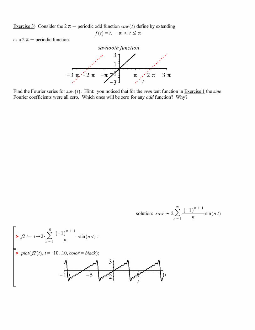
Exercise 3) Consider the 2 periodic odd function saw t define by extending f t = t, t

as a 2 periodic function.

t3 2 2 3

3113

sawtooth function

Find the Fourier series for saw t . Hint: you noticed that for the even tent function in Exercise 1 the sine Fourier coefficients were all zero. Which ones will be zero for any odd function? Why?

solution: saw 2n = 1

1 n 1

nsin n t

f2 t 2n = 1

101 n 1

nsin n t :


t10 5 5 102

3

> >

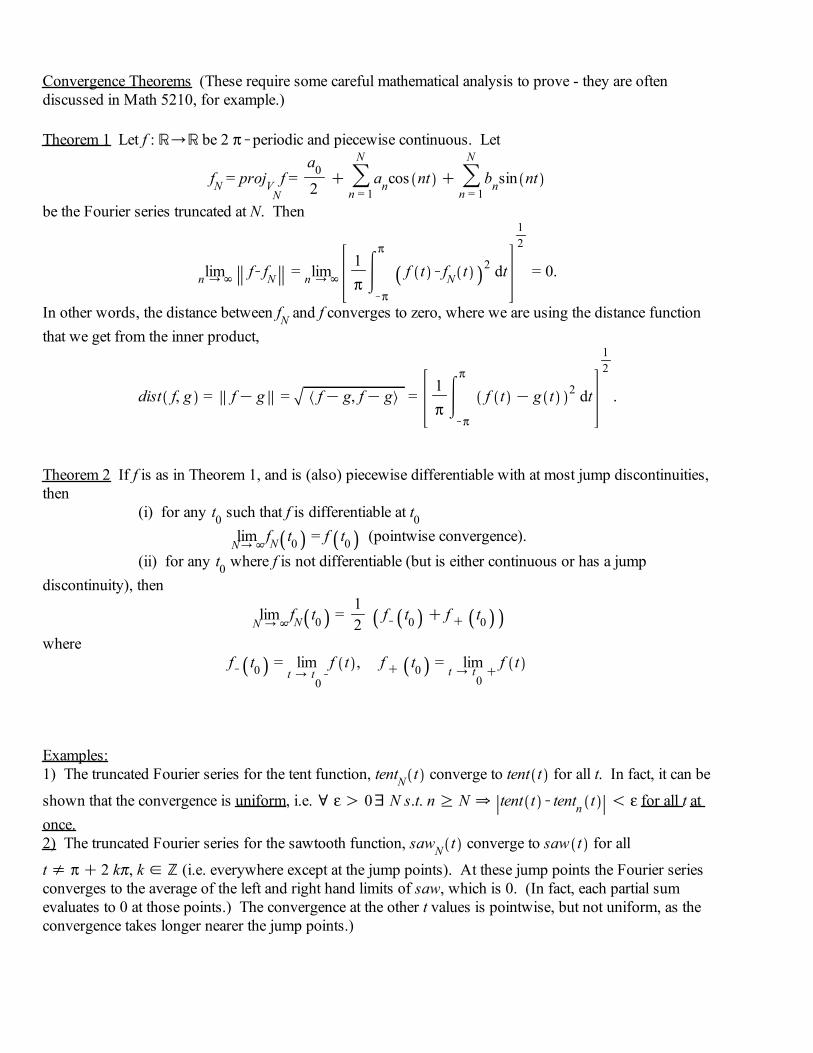
Convergence Theorems (These require some careful mathematical analysis to prove - they are often discussed in Math 5210, for example.)

Theorem 1 Let f : be 2 periodic and piecewise continuous. Let

fN = projVNf =

a0

2 n = 1

N

ancos ntn = 1

N

bnsin nt

be the Fourier series truncated at N. Then

limn f fN = limn1

f t fN t 2 dt

12

= 0.

In other words, the distance between fN and f converges to zero, where we are using the distance function that we get from the inner product,

dist f, g = f g = f g, f g =1

f t g t 2 dt

12

.

Theorem 2 If f is as in Theorem 1, and is (also) piecewise differentiable with at most jump discontinuities, then (i) for any t0 such that f is differentiable at t0

limN

fN t0 = f t0 (pointwise convergence). (ii) for any t0 where f is not differentiable (but is either continuous or has a jump discontinuity), then

limN

fN t0 =12

f t0 f t0where

f t0 = limt t

0

f t , f t0 = limt t

0f t

Examples: 1) The truncated Fourier series for the tent function, tentN t converge to tent t for all t. In fact, it can be

shown that the convergence is uniform, i.e. 0 N s.t. n N tent t tentn t for all t at once.2) The truncated Fourier series for the sawtooth function, sawN t converge to saw t for all

t 2 k , k (i.e. everywhere except at the jump points). At these jump points the Fourier series converges to the average of the left and right hand limits of saw, which is 0. (In fact, each partial sum evaluates to 0 at those points.) The convergence at the other t values is pointwise, but not uniform, as the convergence takes longer nearer the jump points.)

> >

Exercise 4) We can derive "magic" summation formulas using Fourier series. (See your homework for some more.) From Theorem 2 we know that the Fourier series for tent t converges for all t. In particular

0 = tent 0 =2

4n odd

1n2 cos n 0 .

4a) Deduce

11

132

152 ... =

n odd

1n2 =

2

8.

4b) Verify and use

n = 1

1n2 =

n odd

1n2 n even

1n2

=n odd

1n2

14 n = 1

1n2

to show

n = 1

1n2 =

2

6.

> >

Differentiating Fourier Series:

Theorem 3 Let f be 2 periodic, piecewise differentiable and continuous, and with f piecewise continuous. Let f have Fourier series

fa0

2 n = 1ancos n t

n = 1bnsin n t .

Then f has the Fourier series you'd expect by differentiating term by term:

fn = 1

n ansin n tn = 1

n bncos n t

proof: Let f have Fourier series

fA0

2 n = 1Ancos n t

n = 1Bnsin n t .

Then

An =1

f t cos n t dt, n .

Integrate by parts with u = cos n t , dv = f t dt, du = n sin n t dt, v = f t :

1f t cos n t dt =

1f t n sin nt

1f t n sin n t dt

= 0n

f t sin n t dt = n bn.

Similarly, A0 = 0, Bn = n an.

Remark: This is analogous to what happened with Laplace transform. In that case, the transform of the derivative multiplied the transform of the original function by s (and there were correction terms for the initial values). In this case the tranformed variables are the an, bn which depend on n. And the Fourier series "transform" of the derivative of a function multiplies these coefficients by n (and permutes them).

> >

> >

> >

> >

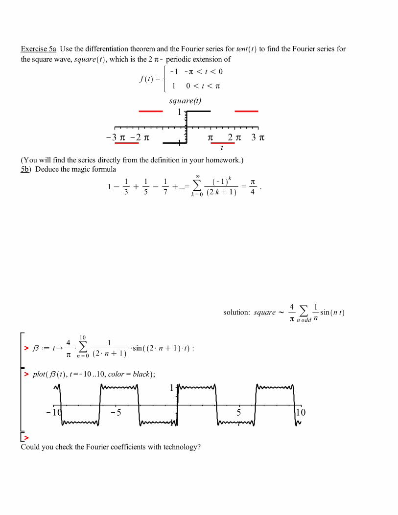
Exercise 5a Use the differentiation theorem and the Fourier series for tent t to find the Fourier series for the square wave, square t , which is the 2 periodic extension of

f t =1 t 0

1 0 t

t3 2 2 3 1

1square(t)

(You will find the series directly from the definition in your homework.)5b) Deduce the magic formula

113

15

17

...=k = 0

1 k

2 k 1=

4 .

solution: square4

n odd

1n

sin n t

f3 t4

n = 0

101

2 n 1sin 2 n 1 t :


t10 5 5 10

1

1

Could you check the Fourier coefficients with technology?

math 2280-001 week 13 april 10-14

Documents