math 2280 - assignment 5 - math - the university of...

Math 2280 - Assignment 5

Dylan Zwick

Fall 2013

Section 3.4 - 1, 5, 18, 21

Section 3.5 - 1, 11, 23, 28, 35, 47, 56

Section 3.6 - 1, 2, 9, 17, 24

1

Section 3.4 - Mechanical Vibrations

3.4.1 - Determine the period and frequency of the simple harmonic motionof a 4-kg mass on the end of a spring with spring constant 16N/m.

Solution - The differential equation 4x′′ + 16x = 0 can be rewritten asx′′ + 4x = 0. This gives us ω2 = 4, and so the angular frequency isω = 2. From this we get the frequency and the period are:

f =2

2π=

1

π,

T =1

f=

11π

= π.

2

3.4.5 - Assume that the differential equation of a simple pendulum oflength L is Lθ′′ + gθ = 0, where g = GM/R2 is the gravitationalacceleration at the location of the pendulum (at distance R from thecenter of the earth; M denotes the mass of the earth).

Two pendulums are of lengths L1 and L2 and - when located at therespective distances R1 and R2 from the center of the earth - haveperiods p1 and p2. Show that

p1

p2=

R1

√L1

R2

√L2

.

Solution - The differential equation governing the motion of our pen-dulum is:

θ′′ +g

Lθ = 0.

From this we get ω =

√

g

L, and so the period is T =

2π

ω= 2π

√

L

g.

Ther period of pendulum 1 will therefore be:

p1 = 2π

√

L1

GM

R2

1

= 2π

√

L1R21

GM.

Similarly, the period of pendulum 2 will be:

p2 = 2π

√

L2R22

GM.

So, the ratio is:

p1

p2

=2πR1

√L1√

GM

2πR2

√L2√

GM

=R1

√L1

R2

√L2

.

3

3.4.18 - A mass m is attached to both a spring (with spring constant k)and a dashpot (with dampring constant c). The mass is set in motionwith initial position x0 and initial velocity v0. Find the position func-tion x(t) and determine whether the motion is overdamped, criticallydamped, or underdamped. If it is underdamped, write the positionfunction in the form x(t) = C1e

−pt cos (ω1t − α1). Also, find the un-damped position function u(t) = C0 cos (ω0t − α0) that would resultif the mass on the spring were set in motion with the same initialposition and velocity, but with the dashpot disconnected (so c = 0).Finally, construct a figure that illustrates the effect of damping bycomparing the graphs of x(t) and u(t).

m = 2, c = 12, k = 50,

x0 = 0, v0 = −8.

Solution - The discriminant of the characteristic polynomial is:

c2 − 4mk = 122 − 4(2)(50) = 144 − 400 = −256 < 0.

So, the motion will be underdamped. The roots of the characteristicpolynomial:

2r2 + 12r + 50

are (using the quadratic equation):

r =−12 ±

√−256

2(2)= −3 ± 4i.

So, the solution is:

4

x(t) = c1e−3t cos (4t) + c2e

−3t sin (4t).

Plugging in the initial conditions we have:

x(0) = c1 = 0,

and therefore

x′(t) = −3c2e−3t sin (4t) + 4c2e

−3t cos (4t)

⇒ x′(0) = 4c2 = −8 ⇒ c2 = −2.

So,

x(t) = −2e−3t sin (4t),

which we can write as:

x(t) = −2e−3t cos(

4t −π

2

)

.

Now, without damping we would get

ω0 =

√

k

m=

√

50

2= 5,

and our solution would be:

u(t) = c1 cos (5t) + c2 sin (5t).

5

Ifwepluginu(O) = Oweget:

u’(t) = 5c2 cos (4t),

and so u’(O) = 5c2 = —8 = c2 = Therefore, the undamped

motion would be:

u(t) — sin (5t) = — cos (5t—

The graphs of these two functions (damped and undamped) looklike:

6

3.4.21 - Same as problem 3.4.18, except with the following values:

m = 1, c = 10, k = 125,

x0 = 6, v0 = 50.

Solution - The characteristic equation for this system will be:

r2 + 10r + 25

which has roots:

r =−10 ±

√

102 − 4(1)(125)

2= −5 ± 10i.

So, our solution is:

x(t) = e−5t(c1 cos (10t) + c2 sin (10t)),

with

x′(t) = 10e−5t(−c1 sin (10t) + c2 cos (10t)) − 5e−5t(c1 cos (10t) + c2 sin (10t)).

If we plug in our initial conditions we get:

x(0) = c1 = 6,

and

x′(0) = 10c2 − 5c1 = 10c2 − 30 = 50 ⇒ c2 = 8.


x(t) = e−5t(6 cos (10t) + 8 sin (10t)).

7

We can rewrite this as:

10e−5t

(

3

5cos (10t) +

4

5sin (10t)

)

= 10e−5t cos (10t − α),

where α = tan−1

(

4

3

)

.

As for the undamped case we have:

ω =

√

125

1= 5

√5.


u(t) = c1 cos (5√

5t) + c2 sin (5√

5t),

u′(t) = −5√

5c1 sin (5√

5t) + 5√

5c2 cos (5√

5t).

If we plug in the initial conditions we get:

u(0) = c1 = 6,

u′(0) = 5√

5c2 = 50 ⇒ c2 = 2√

5.


u(t) = 6 cos (5√

5t) + 2√

5 sin (5√

5t).

Writing this as just a cosine function we get that the amplitude is:

C =

√

62 + (2√

5)2 =√

36 + 20 =√

56 = 2√

14,

α = tan−1

(

2√

5

6

)

.

8

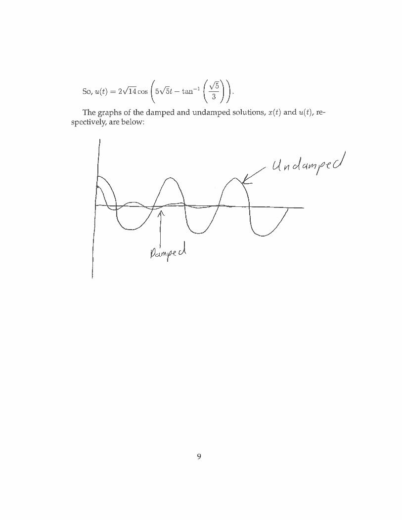
So, (t) = 2cos (5t — taif’ (v)).The graphs of the damped and undamped solutions, x(t) and ‘u(t), re

spectively, are below:

J

9

Section 3.5 - Nonhomogeneous Equations and Un-

determined Coefficients

3.5.1 - Find a particular solution, yp, to the differential equation

y′′ + 16y = e3x.

Solution - We guess the solution will be of the form:

yp = Ae3x,

y′p = 3Ae3x,

y′′p = 9Ae3x.

Plugging these into the ODE we get:

y′′p + 16yp = 25Ae3x = e3x.

So, A =1

25, and we get:

yp =1

25e3x.

10

3.5.11 - Find a particular solution, yp, to the differential equation

y(3) + 4y′ = 3x − 1.

Solution - The corresponding homogeneous equation is:

y(3) + 4y′ = 0,

which has characteristic polynomial:

r3 + 4r = r(r2 + 4).

The roots of this polynomial are r = 0,±2i, and the correspondinghomogeneous solution is:

yh = c1 + c2 sin (2x) + c3 cos (2x).

Now, our initial “guess” for the form of the particular solution wouldbe:

yp = Ax + B.

However, the two terms here are not linearly independent of the ho-mogeneous solution, and so we need to multiply our guess by x toget:

yp = Ax2 + Bx.

From here we get:

11

y′p = 2Ax + B,

y′′p = 2A,

y(3)p = 0.

Plugging these into our ODE we get:

0 + 8Ax + 4B = 3x − 1.

From this we get A =3

8, and B = −

1

4. So, our particular solution is:

yp =3

8x2 −

1

4x.

12

3.5.23 - Set up the appropriate form of a particular solution yp, but do notdetermine the values of the coefficients.1

y′′ + 4y = 3x cos 2x.


y′′ + 4y = 0.

The characteristic polynomial is:

r2 + 4,

which has roots ±2i. So, the form of the homogeneous solution is:

y(x) = c1 sin (2x) + c2 cos (2x).

Now, the guess for our particular solution would be:

yp(x) = (Ax + B) sin (2x) + (Cx + D) cos (2x).

This guess is, however, not independent of our homogeneous solu-tion, and so we must multiply it by x to get:

yp = (Ax2 + Bx) sin (2x) + (Cx2 + Dx) cos (2x).

1Unless you really, really want to.

13

3.5.28 - Same instructions as Problem 3.5.23, but with the differential equa-tion

y(4) + 9y′′ = (x2 + 1) sin 3x.


y(4) + 9y′′ = 0.

The characteristic polynomial for this differential equation is:

r4 + 9r2 = r2(r2 + 9).

This polynomial has roots r = 0, 0,±3i. So, the homogeneous solu-tion has the form:

yh = c1 + c2x + c3 sin (3x) + c4 cos (3x).

Our initial “guess” for the particular solution would be:

yp = (Ax2 + Bx + C) sin (3x) + (Dx2 + Ex + F ) cos (3x).

However, the terms here would not be independent of the homoge-neous solution, and so we must multiply our guess by x to get:

yp = (Ax3 + Bx2 + Cx) sin (3x) + (Dx3 + Ex2 + Fx) cos (3x).

14

3.5.35 - Solve the initial value problem

y′′ − 2y′ + 2y = x + 1;

y(0) = 3, y′(0) = 0.


y′′ − 2y′ + 2y = 0.


r2 − 2r + 2.

This quadratic has roots r =2 ±

√

(−2)2 − 4(1)(2)

2= 1 ± i. So, the

general form of the homogeneous solution is:

yh = c1ex cos (x) + c2e

x sin (x).

Our “guess” for the particular solution will be:

yp = Ax + B,

with

y′p = A,

y′′p = 0.

Plugging these into our differential equation we get:

15

0 − 2A + 2(Ax + B) = x + 1.

Equating coefficients we get A =1

2, B = 1. So,

yp =1

2x + 1.

Therefore, the general form of our solution is:

y = yh + yp = c1ex cos (x) + c2e

x sin (x) +1

2x + 1,

y′ = (c1 + c2)ex cos (x) + (c2 − c1)e

x sin (x) +1

2.

Plugging in our initial conditions we get:

y(0) = 3 = c1 + 1,

y′(0) = 0 = c1 + c2 +1

2.

Solving this system we get c1 = 2, c2 = −5

2. So, our solution is:

y(x) = 2ex cos (x) −5

2ex sin (x) +

1

2x + 1.

16

3.5.47 - Use the method of variation of parameters to find a particular so-lution to the differential equation

y′′ + 3y′ + 2y = 4ex.


y′′ + 3y′ + 2y = 0.

This homogeneous equation has characteristic polynomial:

r2 + 3r + 2 = (r + 2)(r + 1).

The roots of this polynomial are r = −1,−2, and so the general formof the homogeneous solution is:

yh = c1e−2x + c2e

−x.

The corresponding Wronskian is:

W (e−2x, e−x) =

∣

∣

∣

∣

e−2x e−x

−2e−2x −e−x

∣

∣

∣

∣

= e−3x.

Using the method of variation of parameters to get a particular solu-tion we have:

yp = −e−2x

∫

e−x(4ex)

e−3xdx + e−x

∫

e−2x(4ex)

e−3xdx

= −4e−2x

∫

e3xdx + 4e−x

∫

e2xdx = −4

3ex + 2ex =

2

3ex.

17

We can quickly check this:

2

3ex + 3

(

2

3ex

)

+ 2

(

2

3ex

)

= 4ex.

18

3.5.56 - Same instructions as Problem 3.5.47, but with the differential equa-tion

y′′ − 4y = xex.


y′′ − 4y = 0.


r2 − 4 = (r − 2)(r + 2).

The roots of this polynomial are r = ±2, and so the general form ofthe homogeneous solution is:

yh = c1e2x + c2e

−2x.

The corresponding Wronskian is:

W (e2x, e−2x) =

∣

∣

∣

∣

e2x e−2x

2e2x −2e−2x

∣

∣

∣

∣

= −4.

Using the method of variation of parameters to get a particular solu-tion we have:

19

yp = −e2x

∫

e−2x(xex)

−4dx + e−2x

∫

e2x(xex)

−4dx

=1

4

(

e2x

∫

xe−xdx − e−2x

∫

xe3xdx

)

=1

4

(

e2x(

−xe−x − e−x)

− e−2x

(

1

3xe3x −

1

9e3x

))

=1

4

(

−xex − ex −1

3xex +

1

9ex

)

= −1

3xex −

2

9ex.

20

Section 3.6 - Forced Oscillations and Resonance

3.6.1 - Express the solution of the initial value problem

x′′ + 9x = 10 cos 2t;

x(0) = x′(0) = 0,

as a sum of two oscillations in the form:

x(t) = C cos (ω0t − α) +F0/m

ω20 − ω2

cos ωt.


x′′ + 9x = 0,

which has characteristic polynomial:

r2 + 9

The roots of this polynomial are r = ±3i, and so the general form ofthe homogeneous solution is:

xh = c1 cos (3t) + c2 sin (3t).

As for the particular solution, we guess it’s of the form:

xp = A cos (2t) + B sin (2t).

21

The corresponding derivatives are:

x′p = −2A sin (2t) + 2B cos (2t),

x′′p = −4A cos (2t) − 4B sin (2t).


x′′p + 9xp = 5A cos (2t) + 5B sin (2t) = 10 cos (2t).

So,A = 2, B = 0, and

xp = 2 cos (2t).

So, the general solution will be:

x(t) = c1 cos (3t) + c2 sin (3t) + 2 cos (2t),

with

x′(t) = −3c1 sin (3t) + 3c2 cos (3t) − 4 sin (2t).

Plugging in our initial conditions gives us:

x(0) = 0 = 2 + c1

x′(0) = 0 = 3c2.

So, c1 = −2, c2 = 0, and our solution is:

x(t) = −2 cos (3t) + 2 cos (2t).

This is already in the proper form.

22

3.6.2 - Same instructions as Problem 3.6.1, but with the initial value prob-lem:

x′′ + 4x = 5 sin 3t;

x(0) = x′(0) = 0.


x′′ + 4x = 0.

The characteristic polynomial for this equation is:

r2 + 4 = 0,

which has roots r = ±2i. So, the general form of the homogeneoussolution is:

xh = c1 cos (2t) + c2 sin (2t).

As for the particular solution, we guess it’s of the form:

xp = A cos (3t) + B sin (3t),

with corresponding derivatives

x′p = −3A sin (3t) + 3B cos (3t),

x′′p = −9A cos (3t) − 9B sin (3t).

23


x′′p + 4xp = −5A cos (3t) − 5B sin (3t) = 5 sin (3t).

So, A = 0, B = −1, and our particular solution is:

xp = − sin (3t).

Our general solution is then:

x(t) = xh + xp = c1 cos (2t) + c2 sin (2t) − sin (3t),

with corresponding derivative

x′(t) = −2c1 sin (2t) + 2c2 cos (2t) − 3 cos (3t).

Plugging in our initial conditions we get:

x(0) = 0 = c1

x′(0) = 0 = 2c2 − 3.

So, c1 = 0, c2 =3

2, and our solution is:

x(t) =3

2sin (2t) − sin (3t).

Using the identity cos(

x − π2

)

= sin (x) we can convert this to thedesired form:

x(t) =3

2cos(

2t −π

2

)

− cos(

3t −π

2

)

.

24

3.6.9 - Find the steady periodic solution xsp(t) = C cos (ωt− α) of thegiven equation mx′′ + cx′ + kx = F (t) with periodic forcing functionF (t) of frequency ω. Then graph xsp(t) together with (for compari-son) the adjusted forcing function F1(t) = F (t)/mω.

2x′′ + 2x′ + x = 3 sin 10t.

Solution - We first note the the corresponding homogeneous equationis:

2x′′ + 2x′ + x = 0,

which has characteristic polynomial

2r2 + 2r + 1,

with roots r =−2 ±

√

22 − 4(2)(1)

2(2)= −

1

2±

1

2i.

So, the general form of the homogeneous solution is:

xh = c1e− 1

2t cos

(

1

2t

)

+ c2e− 1

2t sin

(

1

2t

)

.

The steady periodic solution is a particular solution, and our “guess”for the particular solution is:

xsp = A cos (10t) + B sin (10t).

These terms are linearly independent of our homogeneous solution,so this is a good guess. Its corresponding derivatives are:

25

x′sp = −10A sin (10t) + 10B cos (10t),

x′′sp = −100A cos (10t) − 100B sin (10t).

Plugging these into our ODE we get:

2x′′sp + 2x′

sp + xsp =(−200A+20B+A) cos (10t)+(−200B−20A+B) sin (10t) = 3 sin (10t).

From these we get the pair of linear equations:

−199A + 20B = 0,

−20A + 199B = 3.

The solution to this system is:

A = −60

40001,

B = −597

40001.

So,

xsp = −1

40001(60 cos (10t) + 597 sin (10t)).

To express this in the proper form we have:

C =

√

(

−60

40001

)2

+

(

−597

40001

)2

=

√

360009

400012=

3√40001

,

26

and

597\ 199”= tan’ (z60j +taif’

So,

= Ccos (lot —

3with C =

____

and c ir + tan1 1199”

v’40001

Graph: (Sketch)

.o,i

27

3.6.17 - Suppose we have a forced mass-spring-dashpot system with equa-tion:

x′′ + 6x′ + 45x = 50 cosωt.

Investigate the possibility of practical resonance of this system. Inparticular, find the amplitude C(ω) of steady periodic forced oscilla-tions with frequency ω. Sketch the graph of C(ω) and find the prac-tical resonance frequency ω (if any).

Solution - Using the equation for C(ω) from section 3.6 of the text-book:

C(ω) =F0

√

(k − mω2)2 + (cω)2,

with F0 = 50, m = 1, c = 6, and k = 45 we get:

C(ω) =50

√

(45 − ω2)2 + (6ω)2.

We get practical resonance when C(ω) is maximized, which will bewhen the denominator is minimized. The denominator will be min-imized when

(45 − ω2)2 + (6ω)2 = w4 − 54ω2 + 2025 = B(ω)

is minimized. Taking this functions first and second derivatives givesus:

B′(ω) = 4ω3 − 108ω = (4ω2 − 108)ω,

B′′(ω) = 12ω2 − 108.

28

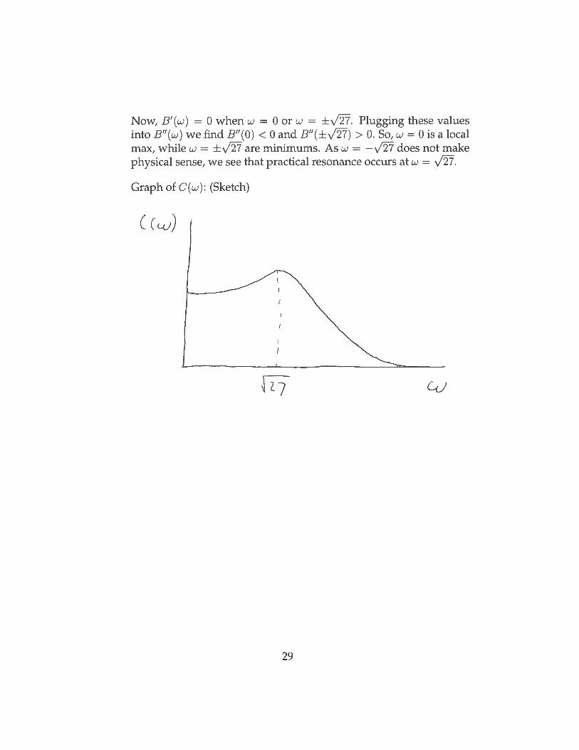
Now, B’(w) = 0 when w = 0 or w = ±\/. Plugging these valuesinto B”(w) we find B”(O) < 0 and B”(+\/) > 0. So, w 0 is a localmax, while w = are minimums. As w = —\/ does not makephysical sense, we see that practical resonance occurs at w =

Graph of C(w): (Sketch)

C)

-LI

29

3.6.24 - A mass on a spring without damping is acted on by the externalforce F (t) = F0 cos3 ωt. Show that there are two values of ω for whichresonance occurs, and find both.

Solution - Using the trigonometric identity

cos2(θ) =1 + cos (2θ)

2

we have

F0 cos3 (ωt) =F0 cos (ωt) + F0 cos (ωt) cos (2ωt)

2.

If we use the trigonometric identity

cos (A) cos (B) =cos (A + B) + cos (A − B)

2

we get:

F0 cos (ωt) + F0 cos (ωt) cos (2ωt)

2=

3F0 cos (ωt)

4+

F0 cos (3ωt)

4.

So, resonance occurs when

√

k

m= ω or

√

k

m= 3ω.

30

math 2280 - assignment 5 - math - the university of...

Documents