maxentropic and quantitative methods in operational risk modeling

MAXENTROPIC AND QUANTITATIVE METHODS INOPERATIONAL RISK MODELING

Erika [email protected]

joint work withSilvia Mayoral Henryk Gzyl

Department of Business AdministrationUniversidad Carlos III de Madrid

September, 2016

1 / 48

Outline

Work Review

(P1) Two Maxentropic Approaches to determine the probability density ofcompound losses. Journal of Insurance: Mathematics and Economics, 2015

(P2) Density Reconstructions with Errors in the Data. Entropy, 2014

(P3) Maxentropic approach to decompound aggregate risk losses. Journal of

Insurance: Mathematics and Economics, 2015

(P4) Loss data analysis: Analysis of the sample dependence in densityreconstruction by maxentropic methods. Journal of Insurance: Mathematics and Economics, 2016

(P5) Maximum entropy approach to the loss data aggregation problem. Journal of

Operational Risk, 2016.

2 / 48

Outline

1 Introduction

MotivationMethodology: Loss distribution Approach

Univariate caseMultivariate case

2 Maximum Entropy Approach

Examples and ApplicationsTheory

3 Numerical Results

4 Conclusions

3 / 48

IntroductionMotivation

Banks developed a conceptual framework to characterize and quantify risk, toput money aside to cover large-scale losses and to ensure the stability of thefinancial system.

In this sense, a similar problem appears also in Insurance, to set premiums andoptimal reinsurance levels.

The differences between these two sectors lies in the availability of the data. InOperational risk the size of the historical data is small. So, the results may varywidely.

More precisely, we are interested in the calculation of regulatory/economiccapital using advanced models (LDA: loss distribution approach) allowed byBasel II.

The problem is the calculation of the amount of money you may need in orderto be hedged at a high level of confidence (VaR: 99,9%).

The regulation states that the allocated capital charge should correspond to a1-in-1000 (quantile .999) years worst possible loss event.

It is necessary to calculate the distribution of the losses, and the methodologyused has to take in consideration challenges related with size of the data sets,bimodality, heavy tails, dependence, between others.

We propose to model the total losses by maximizing an entropy measure.

4 / 48

IntroductionLoss distribution Approach (LDA): Univariate Case

Operational risk has to do withlosses due failures in processes,technology, people, etc.

Two variables play a role in operational risk:

Severity (X ): Lognormal, gamma,weibull distributions, Subexponentialdistributions...

Frequency (N): Poisson, negativebinomial , binomial distributions.

S = X1 + X2 + ...+ XN =N∑

n=1

Xn

where S represents the aggregate claimamount in a fixed time period (typically oneyear) per risk event.

Approach used: Fit parametric distributionsto N and X and obtain fS through recursivemodels or convolutionsNo single distribution fits well over the en-tire data set.

5 / 48

IntroductionLoss distribution Approach (LDA): Multivariate Case

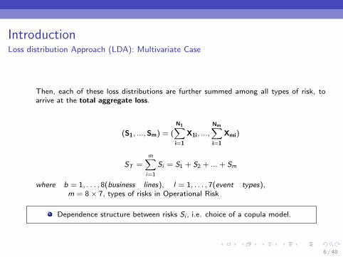
Then, each of these loss distributions are further summed among all types of risk, toarrive at the total aggregate loss.

(S1, ...,Sm) = (

N1∑i=1

X1i, ...,

Nm∑i=1

Xmi)

ST =m∑i=1

Si = S1 + S2 + ...+ Sm

where b = 1, . . . , 8(business lines), l = 1, . . . , 7(event types),m = 8× 7, types of risks in Operational Risk

Dependence structure between risks Si , i.e. choice of a copula model.

6 / 48

IntroductionLoss distribution Approach (LDA): Illustrative Example

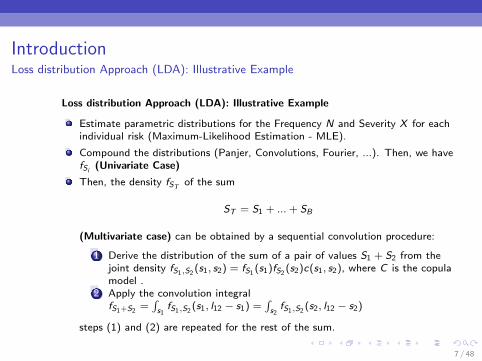
Loss distribution Approach (LDA): Illustrative Example

Estimate parametric distributions for the Frequency N and Severity X for eachindividual risk (Maximum-Likelihood Estimation - MLE).

Compound the distributions (Panjer, Convolutions, Fourier, ...). Then, we havefSi (Univariate Case)

Then, the density fST of the sum

ST = S1 + ...+ SB

(Multivariate case) can be obtained by a sequential convolution procedure:

1 Derive the distribution of the sum of a pair of values S1 + S2 from thejoint density fS1,S2

(s1, s2) = fS1(s1)fS2

(s2)c(s1, s2), where C is the copulamodel .

2 Apply the convolution integralfS1+S2

=∫s1fS1,S2

(s1, l12 − s1) =∫s2fS1,S2

(s2, l12 − s2)

steps (1) and (2) are repeated for the rest of the sum.

7 / 48

IntroductionIllustrative Example

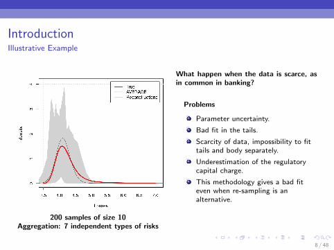
200 samples of size 10Aggregation: 7 independent types of risks

What happen when the data is scarce, asin common in banking?

Problems

Parameter uncertainty.

Bad fit in the tails.

Scarcity of data, impossibility to fittails and body separately.

Underestimation of the regulatorycapital charge.

This methodology gives a bad fiteven when re-sampling is analternative.

8 / 48

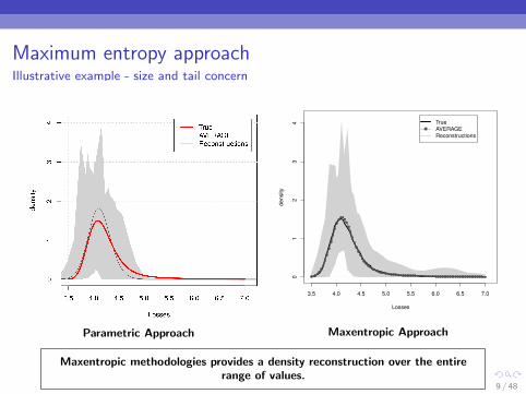
Maximum entropy approachIllustrative example - size and tail concern

Parametric Approach

3.5 4.0 4.5 5.0 5.5 6.0 6.5 7.00

12

34

Losses

density

True

AVERAGE

Reconstructions

Maxentropic Approach

Maxentropic methodologies provides a density reconstruction over the entirerange of values.

9 / 48

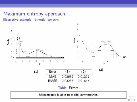
Maximum entropy approachIllustrative example - bimodal concern

(1)(2)

Error (1) (2)

MAE 0.02652 0.01291RMSE 0.03286 0.01647

Table: Errors.

Maxentropic is able to model asymmetries.

10 / 48

Maximum entropy approachDependencies

We use maxentropic methodologies to model dependencies between differenttypes of risks in the framework of Operational risk

11 / 48

Maximum entropy approach

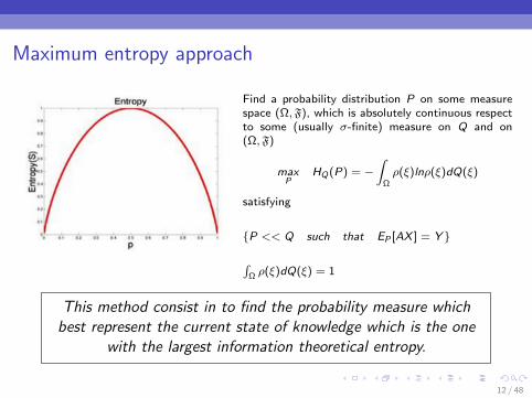
Find a probability distribution P on some measurespace (Ω,F), which is absolutely continuous respectto some (usually σ-finite) measure on Q and on(Ω,F)

maxP

HQ(P) = −∫

Ωρ(ξ)lnρ(ξ)dQ(ξ)

satisfying

P << Q such that EP [AX ] = Y

∫Ω ρ(ξ)dQ(ξ) = 1

This method consist in to find the probability measure whichbest represent the current state of knowledge which is the one

with the largest information theoretical entropy.

12 / 48

Maximum entropy approachJaynes, 1957

This concept was used by Jaynes (1957) for first time as a methodof statistical inference in the case of a under-determined problem.

For example:We rolled 1000 times, a six-sided die comes up with an average of4.7 dots. We want to estimate, as best we can, the probabilitydistribution of the faces.

There are infinitely many 6-tuples (p1, ..., p6) with pi ≥ 0,∑ipi = 1 and

∑iipi = 4.7

13 / 48

Maximum Entropy ApproachGeneral overview

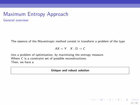
The essence of the Maxentropic method consist in transform a problem of the type

AX = Y X : Ω→ C

into a problem of optimization, by maximizing the entropy measure.Where C is a constraint set of possible reconstructions.Then, we have a

Unique and robust solution

14 / 48

Laplace Transform

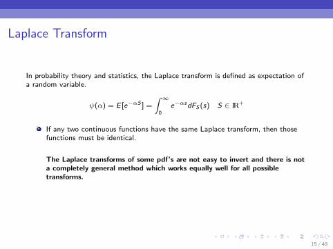
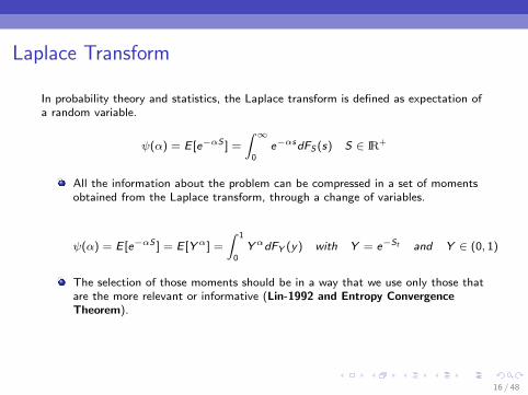
In probability theory and statistics, the Laplace transform is defined as expectation ofa random variable.

ψ(α) = E [e−αS ] =

∫ ∞0

e−αsdFS (s) S ∈ IR+

If any two continuous functions have the same Laplace transform, then thosefunctions must be identical.

The Laplace transforms of some pdf’s are not easy to invert and there is nota completely general method which works equally well for all possibletransforms.

15 / 48

Laplace Transform

In probability theory and statistics, the Laplace transform is defined as expectation ofa random variable.

ψ(α) = E [e−αS ] =

∫ ∞0

e−αsdFS (s) S ∈ IR+

All the information about the problem can be compressed in a set of momentsobtained from the Laplace transform, through a change of variables.

ψ(α) = E [e−αS ] = E [Yα] =

∫ 1

0YαdFY (y) with Y = e−St and Y ∈ (0, 1)

The selection of those moments should be in a way that we use only those thatare the more relevant or informative (Lin-1992 and Entropy ConvergenceTheorem).

16 / 48

Laplace Transform

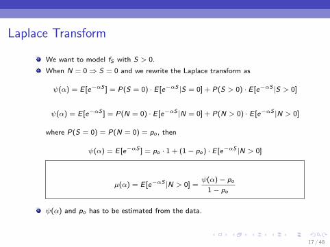
We want to model fS with S > 0.

When N = 0⇒ S = 0 and we rewrite the Laplace transform as

ψ(α) = E [e−αS ] = P(S = 0) · E [e−αS |S = 0] + P(S > 0) · E [e−αS |S > 0]

ψ(α) = E [e−αS ] = P(N = 0) · E [e−αS |N = 0] + P(N > 0) · E [e−αS |N > 0]

where P(S = 0) = P(N = 0) = po , then

ψ(α) = E [e−αS ] = po · 1 + (1− po) · E [e−αS |N > 0]

µ(α) = E [e−αS |N > 0] =ψ(α)− po

1− po

ψ(α) and po has to be estimated from the data.

17 / 48

Input of the MethodologyUnivariate Case

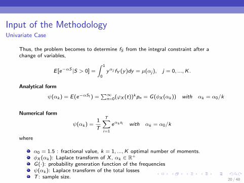
Thus, the problem becomes to determine fS from the integral constraint after achange of variables,

E [e−αS |S > 0] =

∫ 1

0yαj fY (y)dy = µ(αj ), j = 0, ...,K .

Analytical form

ψ(αk ) = E(e−αSt ) =∑∞

n=0(ϕX (t))kpn = G(φX (αk )) with αk = α0/k

Numerical form

ψ(αk ) =1

T

T∑i=1

eαk si with αk = α0/k

where

α0 = 1.5 : fractional value, k = 1, ...,K optimal number of moments.φX (αk ): Laplace transform of X , αk ∈ R+

G(·): probability generation function of the frequenciesψ(αk ): Laplace transform of the total lossesT : sample size.

18 / 48



E [e−αS |S > 0] =

∫ 1

0yαj fY (y)dy = µ(αj ), j = 0, ...,K .

Analytical formFit parametrically the frequency and severity distributions and calculate the Laplacetransform through the probability generation function.Poisson-Gamma

ψ(αk ) = exp(−`(1− ba(αk + b)−a))with αk = α0/k

The quality of the results is linked to how well the data fit to the defineddistributions.

It is not possible to find a closed form of ψ(αk ) for some pdf’s. This isparticular true for long tail pdf’s, as for example the lognormal distribution.

19 / 48



E [e−αS |S > 0] =

∫ 1

0yαj fY (y)dy = µ(αj ), j = 0, ...,K .

Analytical form

ψ(αk ) = E(e−αSt ) =∑∞

n=0(ϕX (t))kpn = G(φX (αk )) with αk = α0/k

Numerical form

ψ(αk ) =1

T

T∑i=1

eαk si with αk = α0/k

where

α0 = 1.5 : fractional value, k = 1, ...,K optimal number of moments.φX (αk ): Laplace transform of X , αk ∈ R+

G(·): probability generation function of the frequenciesψ(αk ): Laplace transform of the total lossesT : sample size.

20 / 48

Input of the MethodologyMultivariate Case Dependencies

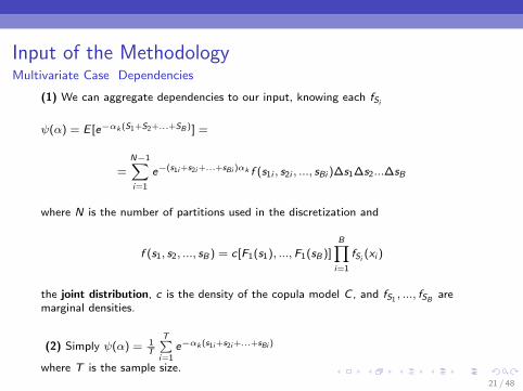
(1) We can aggregate dependencies to our input, knowing each fSi

ψ(α) = E [e−αk (S1+S2+...+SB )] =

=

N−1∑i=1

e−(s1i+s2i+...+sBi )αk f (s1i , s2i , ..., sBi )∆s1∆s2...∆sB

where N is the number of partitions used in the discretization and

f (s1, s2, ..., sB) = c[F1(s1), ...,F1(sB)]B∏i=1

fSi (xi )

the joint distribution, c is the density of the copula model C , and fS1, ..., fSB are

marginal densities.

(2) Simply ψ(α) = 1T

T∑i=1

e−αk (s1i+s2i+...+sBi )

where T is the sample size.

21 / 48

Maximum Entropy Methods

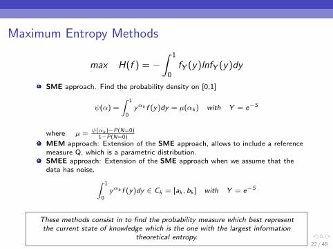
max H(f ) = −∫ 1

0fY (y)lnfY (y)dy

SME approach. Find the probability density on [0,1]

ψ(α) =

∫ 1

0yαk f (y)dy = µ(αk ) with Y = e−S

where µ = ψ(αk )−P(N=0)1−P(N=0)

MEM approach: Extension of the SME approach, allows to include a referencemeasure Q, which is a parametric distribution.SMEE approach: Extension of the SME approach when we assume that thedata has noise. ∫ 1

0yαk f (y)dy ∈ Ck = [ak , bk ] with Y = e−S

These methods consist in to find the probability measure which best representthe current state of knowledge which is the one with the largest information

theoretical entropy.22 / 48

Standard Maximum Entropy Method (SME)

In general, the maximum entropy density is obtained by maximizing the entropymeasure

Max H(f ) = −∫ 1

0fY (y)lnfY (y)dy

satisfying

E(yαk ) =

∫ 1

0yαk fY (y)dy = µαk , k = 1, 2, ...,K with K = 8

∫ 10 fY (y)dy = 1

whereµk : k-th moment, which it is positive and it is a known valueK = 8: number of momentsFractional value: αk = α0/k, α0 = 1.5

23 / 48

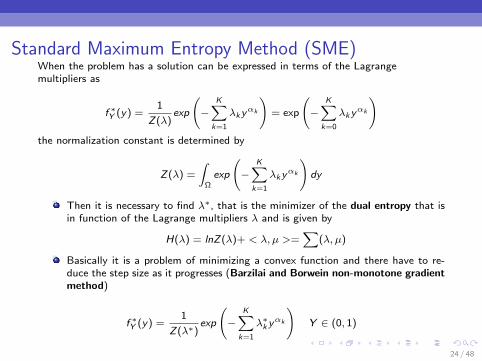
Standard Maximum Entropy Method (SME)When the problem has a solution can be expressed in terms of the Lagrangemultipliers as

f ∗Y (y) =1

Z(λ)exp

(−

K∑k=1

λkyαk

)= exp

(−

K∑k=0

λkyαk

)the normalization constant is determined by

Z(λ) =

∫Ωexp

(−

K∑k=1

λkyαk

)dy

Then it is necessary to find λ∗, that is the minimizer of the dual entropy that isin function of the Lagrange multipliers λ and is given by

H(λ) = lnZ(λ)+ < λ, µ >=∑

(λ, µ)

Basically it is a problem of minimizing a convex function and there have to re-duce the step size as it progresses (Barzilai and Borwein non-monotone gradientmethod)

f ∗Y (y) =1

Z(λ∗)exp

(−

K∑k=1

λ∗k yαk

)Y ∈ (0, 1)

24 / 48

Standard Maximum Entropy Method (SME)1 The starting point is

∫∞0 e−αsdFS (s) = µk , S ∈ (0,∞)

2 Make a change of variables, setting Y = e−S(N), Y ∈ (0, 1),

3 Find a minimum of the dual entropy that is in function of λ,

minλ

∑(λ, µ) = lnZ(λ)+ < λ, µ >

where

Z(λ) =

∫ 1

0e−

∑Kk=1 λk y

αkdy .

4 The solution

f ∗Y (y) =1

Z(λ∗)e−

∑Kk=1 λ

∗k y

αk= e−

∑Kk=0 λ

∗k y

αkY ∈ (0, 1)

5 Return the change of variables

f ∗S (s) = e−s f ∗Y (e−s), S ∈ (0,∞)

25 / 48

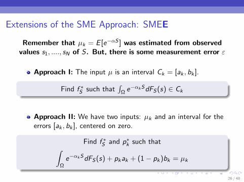
Extensions of the SME Approach: SMEE

Remember that µk = E [e−αS ] was estimated from observedvalues s1, ...., sN of S . But, there is some measurement error ε

Approach I: The input µ is an interval Ck = [ak , bk ].

Find f ∗S such that∫

Ω e−αkSdFS(s) ∈ Ck

Approach II: We have two inputs: µk and an interval for theerrors [ak , bk ], centered on zero.

Find f ∗S and p∗k such that∫Ωe−αkSdFS(s) + pkak + (1− pk)bk = µk

26 / 48

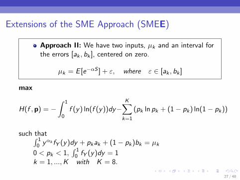
Extensions of the SME Approach (SMEE)

Approach II: We have two inputs, µk and an interval forthe errors [ak , bk ], centered on zero.

µk = E [e−αS ] + ε, where ε ∈ [ak , bk ]

max

H(f ,p) = −∫ 1

0f (y) ln(f (y))dy−

K∑k=1

(pk ln pk + (1− pk) ln(1− pk))

such that∫ 10 yαk fY (y)dy + pkak + (1− pk)bk = µk

0 < pk < 1,∫ 1

0 fY (y)dy = 1k = 1, ...,K with K = 8.

27 / 48

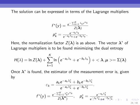
The solution can be expressed in terms of the Lagrange multipliers

f ∗(y) = e−∑K

k=1 λk yαk

Z(λ)

p∗k = e−akλk

e−akλk +e−bkλk.

Here, the normalization factor Z (λ) is as above. The vector λ∗ ofLagrange multipliers is to be found minimizing the dual entropy

H(λ) = lnZ (λ) +K∑

k=1

ln(e−akλk + e−bkλk

)+ < λ,µ >= Σ(λ)

Once λ∗ is found, the estimator of the measurement error is, givenby

εk =ake−akλ∗k + bke

−bkλ∗k

e−akλ∗k + e−bkλ

∗k

.

f ∗(y) = e−∑K

k=1 λ∗k yαk

Z(λ∗), p∗k = e−akλ

∗k

e−akλ

∗k +e

−bkλ∗k

28 / 48

Numerical Results

1 Two Maxentropic Approaches to determine the probability density of compoundlosses.

2 Density Reconstructions with Errors in the Data.

3 Maxentropic approach to decompound aggregate risk losses.

4 Loss data analysis: Analysis of the Sample Dependence in DensityReconstruction by Maxentropic Methods.

5 Maximum entropy approach to the loss data aggregation problem.

29 / 48

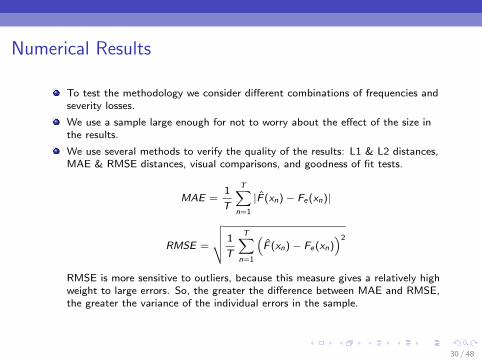
Numerical Results

To test the methodology we consider different combinations of frequencies andseverity losses.

We use a sample large enough for not to worry about the effect of the size inthe results.

We use several methods to verify the quality of the results: L1 & L2 distances,MAE & RMSE distances, visual comparisons, and goodness of fit tests.

MAE =1

T

T∑n=1

|F (xn)− Fe(xn)|

RMSE =

√√√√ 1

T

T∑n=1

(F (xn)− Fe(xn)

)2

RMSE is more sensitive to outliers, because this measure gives a relatively highweight to large errors. So, the greater the difference between MAE and RMSE,the greater the variance of the individual errors in the sample.

30 / 48

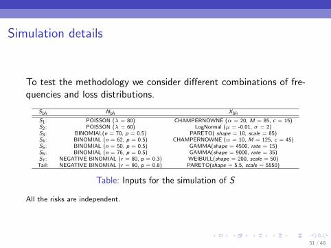
Simulation details

To test the methodology we consider different combinations of fre-quencies and loss distributions.

Sbh Nbh Xbh

S1: POISSON (λ = 80) CHAMPERNOWNE (α = 20, M = 85, c = 15)S2: POISSON (λ = 60) LogNormal (µ = -0.01, σ = 2)S3: BINOMIAL(n = 70, p = 0.5) PARETO( shape = 10, scale = 85)S4: BINOMIAL (n = 62, p = 0.5) CHAMPERNOWNE (α = 10, M = 125, c = 45)S5: BINOMIAL (n = 50, p = 0.5) GAMMA(shape = 4500, rate = 15)S6: BINOMIAL (n = 76, p = 0.5) GAMMA(shape = 9000, rate = 35)S7: NEGATIVE BINOMIAL (r = 80, p = 0.3) WEIBULL(shape = 200, scale = 50)

Tail: NEGATIVE BINOMIAL (r = 90, p = 0.8) PARETO(shape = 5.5, scale = 5550)

Table: Inputs for the simulation of S

All the risks are independent.

31 / 48

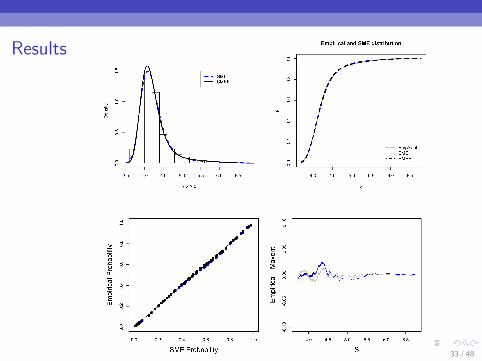
Results

Approach MAE RMSESMEE 0.005928 0.006836SME 0.006395 0.009399

Table: MAE and RMSE for a sample size of5000

MAE =1

T

T∑n=1

|F (xn)− Fe(xn)|

RMSE =

√√√√ 1

T

T∑n=1

(F (xn)− Fe(xn)

)2

32 / 48

Results

33 / 48

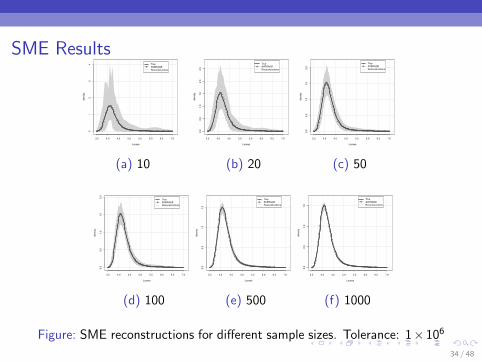
SME Results

3.5 4.0 4.5 5.0 5.5 6.0 6.5 7.0

01

23

4

Losses

de

nsity

True

AVERAGE

Reconstructions

(a) 10

3.5 4.0 4.5 5.0 5.5 6.0 6.5 7.0

0.0

0.5

1.0

1.5

2.0

2.5

Losses

de

nsity

True

AVERAGE

Reconstructions

(b) 20

3.5 4.0 4.5 5.0 5.5 6.0 6.5 7.0

0.0

0.5

1.0

1.5

2.0

Losses

de

nsity

True

AVERAGE

Reconstructions

(c) 50

3.5 4.0 4.5 5.0 5.5 6.0 6.5 7.0

0.0

0.5

1.0

1.5

2.0

Losses

de

nsity

True

AVERAGE

Reconstructions

(d) 100

3.5 4.0 4.5 5.0 5.5 6.0 6.5 7.0

0.0

0.5

1.0

1.5

Losses

de

nsity

True

AVERAGE

Reconstructions

(e) 500

3.5 4.0 4.5 5.0 5.5 6.0 6.5 7.0

0.0

0.5

1.0

1.5

Losses

de

nsity

True

AVERAGE

Reconstructions

(f) 1000

Figure: SME reconstructions for different sample sizes. Tolerance: 1× 106

34 / 48

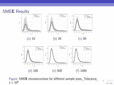
SMEE Results

3.5 4.0 4.5 5.0 5.5 6.0 6.5 7.0

01

23

Losses

de

nsity

True

AVERAGE

Reconstructions

(a) 10

3.5 4.0 4.5 5.0 5.5 6.0 6.5 7.0

0.0

0.5

1.0

1.5

2.0

2.5

Losses

de

nsity

True

AVERAGE

Reconstructions

(b) 20

3.5 4.0 4.5 5.0 5.5 6.0 6.5 7.0

0.0

0.5

1.0

1.5

2.0

Losses

de

nsity

True

AVERAGE

Reconstructions

(c) 50

3.5 4.0 4.5 5.0 5.5 6.0 6.5 7.0

0.0

0.5

1.0

1.5

2.0

Losses

de

nsity

True

AVERAGE

Reconstructions

(d) 100

3.5 4.0 4.5 5.0 5.5 6.0 6.5 7.0

0.0

0.5

1.0

1.5

Losses

de

nsity

True

AVERAGE

Reconstructions

(e) 500

3.5 4.0 4.5 5.0 5.5 6.0 6.5 7.0

0.0

0.5

1.0

1.5

Losses

de

nsity

True

AVERAGE

Reconstructions

(f) 1000

Figure: SMEE reconstructions for different sample sizes. Tolerance:1× 106

35 / 48

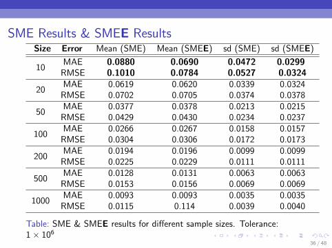
SME Results & SMEE ResultsSize Error Mean (SME) Mean (SMEE) sd (SME) sd (SMEE)

10MAE 0.0880 0.0690 0.0472 0.0299

RMSE 0.1010 0.0784 0.0527 0.0324

20MAE 0.0619 0.0620 0.0339 0.0324

RMSE 0.0702 0.0705 0.0374 0.0378

50MAE 0.0377 0.0378 0.0213 0.0215

RMSE 0.0429 0.0430 0.0234 0.0237

100MAE 0.0266 0.0267 0.0158 0.0157

RMSE 0.0304 0.0306 0.0172 0.0173

200MAE 0.0194 0.0196 0.0099 0.0099

RMSE 0.0225 0.0229 0.0111 0.0111

500MAE 0.0128 0.0131 0.0063 0.0063

RMSE 0.0153 0.0156 0.0069 0.0069

1000MAE 0.0093 0.0093 0.0035 0.0035

RMSE 0.0115 0.114 0.0039 0.0040

Table: SME & SMEE results for different sample sizes. Tolerance:1× 106

36 / 48

SME Results & SMEE ResultsSize Area (SME) Area (SMEE) AVE.(SME) AVE.(SMEE)

10 2.625 2.6190.0092 0.00690.0120 0.0110

20 1.523 1.7590.0082 0.00660.0116 0.0109

50 0.955 1.0440.0082 0.00650.0106 0.0102

100 0.696 0.6900.0053 0.00600.0066 0.0082

200 0.538 0.5520.0053 0.00630.0067 0.0072

500 0.326 0.2940.0055 0.00580.0076 0.0083

1000 0.203 0.2000.0054 0.00570.0078 0.0082

Table: SME & SMEE results for different sample sizes. Tolerance:1× 106

37 / 48

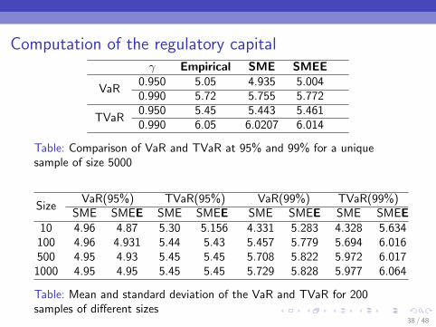
Computation of the regulatory capitalγ Empirical SME SMEE

VaR0.950 5.05 4.935 5.0040.990 5.72 5.755 5.772

TVaR0.950 5.45 5.443 5.4610.990 6.05 6.0207 6.014

Table: Comparison of VaR and TVaR at 95% and 99% for a uniquesample of size 5000

SizeVaR(95%) TVaR(95%) VaR(99%) TVaR(99%)

SME SMEE SME SMEE SME SMEE SME SMEE10 4.96 4.87 5.30 5.156 4.331 5.283 4.328 5.634

100 4.96 4.931 5.44 5.43 5.457 5.779 5.694 6.016500 4.95 4.93 5.45 5.45 5.708 5.822 5.972 6.017

1000 4.95 4.95 5.45 5.45 5.729 5.828 5.977 6.064

Table: Mean and standard deviation of the VaR and TVaR for 200samples of different sizes

38 / 48

Conclusions

In this work we present an application of the maxentropic methodologies toOperational Risk. We showed that this methodology can provide a good densityreconstruction over the entire range, in the case of scarcity, heavy tails andasymmetries, using only eight moments as input of the methodology.

This methodology gives the possibility to obtain the density distributions fromdifferent levels of aggregation and allow us to include dependencies betweendifferent types of risks.

We can joint marginal densities obtained from any methodology and givethem any relation orwe can obtain the joint distribution directly from the data and avoid badestimations

The estimation of the underlying loss process provides a starting point to designpolicies, set premiums and reserves, calculate optimal reinsurance levels andcalculate risk pressures for solvency purposes in insurance and risk management.Also, this is useful in structural engineering to describe the accumulated damageof a structure, just to mention one more possible application.

39 / 48

Conclusions

1 Two Maxentropic Approaches to determine the probability density of compoundlosses.

2 Density Reconstructions with Errors in the Data.

3 Maxentropic approach to decompound aggregate risk losses.

4 Loss data analysis: Analysis of the Sample Dependence in DensityReconstruction by Maxentropic Methods.

5 Maximum entropy approach to the loss data aggregation problem.

40 / 48

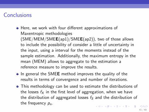
Conclusions

Here, we work with four different approximations ofMaxentropic methodologies(SME/MEM/SMEE(ap1)/SMEE(ap2)), two of those allowsto include the possibility of consider a little of uncertainty inthe input, using a interval for the moments instead of thesample estimation. Additionally, the maximum entropy in themean (MEM) allows to aggregate to the estimation areference measure to improve the results.

In general the SMEE method improves the quality of theresults in terms of convergence and number of iterations.

This methodology can be used to estimate the distributions ofthe losses fX in the first level of aggregation, when we havethe distribution of aggregated losses fS and the distribution ofthe frequency pn.

41 / 48

QUESTIONS, COMMENTS

42 / 48

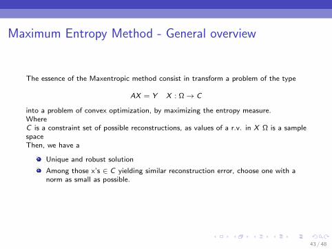
Maximum Entropy Method - General overview

The essence of the Maxentropic method consist in transform a problem of the type

AX = Y X : Ω→ C

into a problem of convex optimization, by maximizing the entropy measure.WhereC is a constraint set of possible reconstructions, as values of a r.v. in X Ω is a samplespaceThen, we have a

Unique and robust solution

Among those x’s ∈ C yielding similar reconstruction error, choose one with anorm as small as possible.

43 / 48

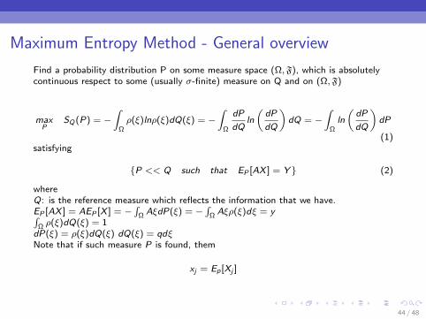
Maximum Entropy Method - General overview

Find a probability distribution P on some measure space (Ω,F), which is absolutelycontinuous respect to some (usually σ-finite) measure on Q and on (Ω,F)

maxP

SQ(P) = −∫

Ωρ(ξ)lnρ(ξ)dQ(ξ) = −

∫Ω

dP

dQln

(dP

dQ

)dQ = −

∫Ωln

(dP

dQ

)dP

(1)satisfying

P << Q such that EP [AX ] = Y (2)

whereQ: is the reference measure which reflects the information that we have.EP [AX ] = AEP [X ] = −

∫Ω AξdP(ξ) = −

∫Ω Aξρ(ξ)dξ = y∫

Ω ρ(ξ)dQ(ξ) = 1dP(ξ) = ρ(ξ)dQ(ξ) dQ(ξ) = qdξNote that if such measure P is found, them

xj = Ep [Xj ]

44 / 48

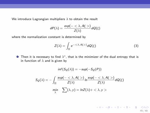
We introduce Lagrangian multipliers λ to obtain the result

dP(λ) =exp(− < λ,Aξ >)

Z(λ)dQ(ξ)

where the normalization constant is determined by

Z(λ) =

∫Ωe−<λ,Aξ>)dQ(ξ) (3)

Then it is necessary to find λ∗, that is the minimizer of the dual entropy that isin function of λ and is given by

inf (SQ(λ)) = −sup(−SQ(P))

SQ(λ) = −∫

Ω

exp(− < λ,Aξ >)

Z(λ)lnexp(− < λ,Aξ >)

Z(λ)dQ(ξ)

minλ

∑(λ, y) = lnZ(λ)+ < λ, y >

45 / 48

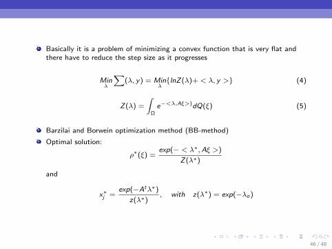
Basically it is a problem of minimizing a convex function that is very flat andthere have to reduce the step size as it progresses

Minλ

∑(λ, y) = Min

λlnZ(λ)+ < λ, y > (4)

Z(λ) =

∫Ωe−<λ,Aξ>)dQ(ξ) (5)

Barzilai and Borwein optimization method (BB-method)

Optimal solution:

ρ∗(ξ) =exp(− < λ∗,Aξ >)

Z(λ∗)

and

x∗j =exp(−Atλ∗)

z(λ∗), with z(λ∗) = exp(−λo)

46 / 48

Measures of Reference

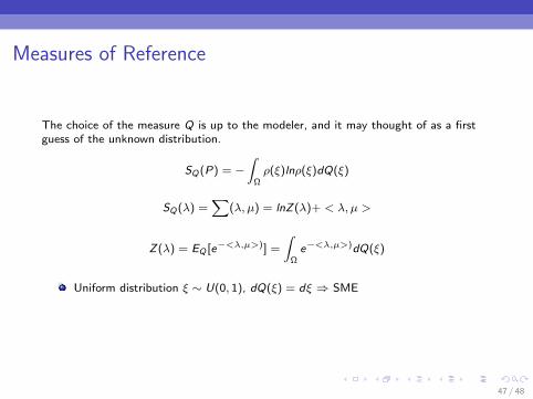
The choice of the measure Q is up to the modeler, and it may thought of as a firstguess of the unknown distribution.

SQ(P) = −∫

Ωρ(ξ)lnρ(ξ)dQ(ξ)

SQ(λ) =∑

(λ, µ) = lnZ(λ)+ < λ, µ >

Z(λ) = EQ [e−<λ,µ>)] =

∫Ωe−<λ,µ>)dQ(ξ)

Uniform distribution ξ ∼ U(0, 1), dQ(ξ) = dξ ⇒ SME

47 / 48

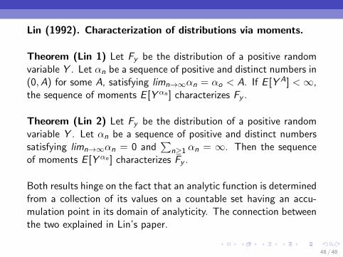
Lin (1992). Characterization of distributions via moments.

Theorem (Lin 1) Let Fy be the distribution of a positive randomvariable Y . Let αn be a sequence of positive and distinct numbers in(0,A) for some A, satisfying limn→∞αn = αo < A. If E [Y A] <∞,the sequence of moments E [Y αn ] characterizes Fy .

Theorem (Lin 2) Let Fy be the distribution of a positive randomvariable Y . Let αn be a sequence of positive and distinct numberssatisfying limn→∞αn = 0 and

∑n≥1 αn = ∞. Then the sequence

of moments E [Y αn ] characterizes Fy .

Both results hinge on the fact that an analytic function is determinedfrom a collection of its values on a countable set having an accu-mulation point in its domain of analyticity. The connection betweenthe two explained in Lin’s paper.

48 / 48

maxentropic and quantitative methods in operational risk modeling

Data & Analytics