modeling operational variability for robust

HAL Id: hal-01534843https://hal-enac.archives-ouvertes.fr/hal-01534843

Submitted on 28 Jun 2017

HAL is a multi-disciplinary open accessarchive for the deposit and dissemination of sci-entific research documents, whether they are pub-lished or not. The documents may come fromteaching and research institutions in France orabroad, or from public or private research centers.

L’archive ouverte pluridisciplinaire HAL, estdestinée au dépôt et à la diffusion de documentsscientifiques de niveau recherche, publiés ou non,émanant des établissements d’enseignement et derecherche français ou étrangers, des laboratoirespublics ou privés.

Modeling Operational Variability for RobustMultidisciplinary Design Optimization

Nicolas Peteilh, Marcel Mongeau, Christian Bes, MélanieConderolle-Lestremau, Thierry Druot

To cite this version:Nicolas Peteilh, Marcel Mongeau, Christian Bes, Mélanie Conderolle-Lestremau, Thierry Druot. Mod-eling Operational Variability for Robust Multidisciplinary Design Optimization. 18th AIAA/ISSMOMultidisciplinary Analysis and Optimization Conference, AIAA AVIATION Forum, Jun 2017, Denver,United States. �10.2514/6.2017-4328�. �hal-01534843�

https://hal-enac.archives-ouvertes.fr/hal-01534843

https://hal.archives-ouvertes.fr

Modeling operational variability for aircraft robust

Multidisciplinary Design Optimization

N. Peteilh∗∗ , M. Mongeau††

ENAC, Universite de Toulouse, France

C. Bes‡‡

Universite Paul Sabatier (UPS), Universite de Toulouse, France

M. Conderolle-Lestremeau§§ , T. Druot¶¶

Airbus, Toulouse, France

The aim of this paper is to model and propagate operational uncertainties in view ofits integration in a multidisciplinary optimization methodology for aircraft robust design.From databases relative to one specific type of long-range airplane, we analyze the variationsof four flight parameters (altitude, speed, temperature and range), and build the associatedstatistical distributions. Then, using an uncertainty propagation methodology, we identifythe distribution of operational costs.

I. Introduction

The need to reduce the environmental impact of air transportation is today widely recognized. The Ad-visory Council for Aviation Research and innovation in Europe (ACARE) has identified energy supplies andthe protection of the environment as key challenges in its Strategic Research and Innovation Agenda1(SRIA).Airplane design is an important mean to meet the sustainable development requirements and, consideringthe development of the civil aviation sector, even a few percentages gained on fuel consumption have astrong impact on the environmental footprint of air transportation. In the last decades, manufacturers havelargely improved airplane design using optimization methodologies. Today, one of the ways to achieve fur-ther significant improvements is to consider the interaction between the airplane and the other air transportsystem stakeholders such as airlines, airports, the passengers, the air traffic management, etc. This papercontributes to the quantification of the interactions between a manufacturer nominal aircraft design and itsoperational use by airlines.

Today, the design of a transport airplane starts with the definition of a set of requirements, which includesthe description of a typical mission representing the anticipated future airplane operations. During the designphases, from the conceptual to the detailed designs, the airplane overall design is optimized with respect tothis specific mission. Nevertheless, when it enters into service a few years later, it is operated by the airlineson their specific networks, according to the timetables and meeting the airlines’ operational needs.

In practice, the missions the airplane has to fly greatly differs from the nominal mission for which it wasoptimized. In addition, the airplane has to face several types of operational variability, related for instance totemperature, altitude, range, payload, or speed. These variabilities are due to operational parameters thatrange from the airlines routes, on-board services, flight load factor, weather conditions (wind, temperatures,and atmospheric pressure), or even to the air navigation service activities. As a consequence, an airplane ishardly ever used for the original mission for which it was initially sized and optimized. Therefore, this mayhave a high impact on the operational costs.

∗PhD Student, Optim research group, 7 avenue Edouard Belin, CS 54005, 31055 Toulouse cedex 4, and AIAA Member†Professor, Optim research group, 7 avenue Edouard Belin, CS 54005, 31055 Toulouse cedex 4.‡Professor, MS2M, Espace Clement Ader, 3 rue Caroline Aigle, 31400 Toulouse, and AIAA Senior Member.§Apprentice engineer, 316 route de Bayonne, 31300 Toulouse.¶Senior Engineer, 316 route de Bayonne, 31300 Toulouse.

1 of 17

American Institute of Aeronautics and Astronautics

The aim of this paper is to model and propagate operational uncertainties in view of its integrationin a multidisciplinary-optimization tool for robust design. The paper is organized as follows. In the firstsection, we make a first analysis from databases that shows the high impact of range variability on costs.Section 2 provides histograms issued from another database that reflects the variability of the main flightparameters. Section 3 deals with the identification of the statistical models underlying these histograms.Section 4 introduces the overall airplane conceptual design model proposed. The last section is dedicatedto the propagation of the statistical distributions of the flight parameters through the conceptual designmodels. More precisely, we estimate the statistical distribution of operational costs resulting from theseinput uncertainties.

II. Preliminary study

The first step of the analysis is to assess whether the different kinds of variability would impact the costper passenger and per nautical mile of a long-range airplane. Based on the OAG database,2 a first analysis iscarried out to confirm the large variety of ranges, and then to assess operational costs. The flights performedby long-range type airplanes such as A330, A340, A350, A380, B747, B777, and B787 are considered over aperiod of one year (2014), representing a total of 2,300,000 flights. The histogram of their range was plottedand analyzed as a whole and in more details for 22 airlines. The graphs presented in Figure 1 show thedistributions (number of flights per range) obtained. The first graph shows that the long-range airplanes areused on a large scale of mission ranges, with a surprisingly-high peak of short-range flights. The three otherhistograms reveal different operational uses by the airlines. Airline 1 uses its long-range airplanes for a largevariety of ranges, while Airline 5 operates them mainly on long-range flights, and Airline 10 flies mainly onshort-range flights.

(a) (b)

(c) (d)

Figure 1. Distributions (number of flights per range) obtained for all the airlines together (a), and for 3 ofthem exhibiting different behaviors: Airline 1 (b), Airline 5 (c) and Airline 10 (d).

Based on these distributions, an evaluation of the cost per passenger and per nautical mile is thenconducted for one specific long-range airplane type over a period of one year (2013) and for 19 airlines. Forconfidentiality reasons, a specific mission is chosen as a reference. Its range is 4000 NM. It corresponds to

2 of 17


the average mission used in the design process. All the costs are presented with respect to the cost of thisreference mission. It is assumed that each flight carries the same number of passengers.

The results presented in Figure 2 show the cost per passenger and nautical mile as a function of the range.It is the Cash Operating Cost (COC) that includes costs related to the flight cycle, such as the maintenanceor the airport taxes. This explains the high increase of costs for the short-range flights.

Figure 2. Average cost per passenger and per nautical miles as a function of range

Knowing the range distribution for each 19 airlines over a period of one year, the average cost is calculatedand presented in Figure 3. The left-hand side part of the graph shows the average cost for each airline, andthe right-hand side part displays an the histogram of the extra cast incurred. All the costs are higher thatthe reference one. It is concluded that the variability on the range impacts the average costs for the airlinesin a negative way.

Figure 3. Average costs per passenger and per nautical miles for the studied airlines. The left-hand side partshows the cost for each airline (designated by a letter), and the right-hand side part presents the distributionof the extra costs.

Based on this first result, we further investigate the effect of variability on the costs.

III. Flight-parameter variability

These results prompt us to broaden the study and to study in more detail the four main flight parameters(temperature, speed, altitude and range) concerning one specific type of long-range airplane over a period

3 of 17


of twenty years.

These four parameters play a key role in the design phase as they affect the quantity of fuel necessary tofly the mission. The way they impact the quantity of fuel burnt during one flight (called block fuel) can bedescribed using the Breguet-Leduc equation of the specific range RS :

RS =L/D V

m g TSFC(1)

where V is the airspeed, TSFC stands for the Thrust Specific Fuel Consumption, L/D for the Lift-to-Dragratio, and g is the gravitational constant (= 9.81m/s2). The specific range can be integrated over the wholeflight, and assuming constant airspeed, thrust specific fuel consumption, and lift-to-drag ratio as well asascending cruise trajectory. The result is the integral expression of Breguet-Leduc equation:

mfuel

MWE +OIW + Payload+ Fuelreserve= exp

(g Range TSFC

V L/D

)− 1 (2)

where MWE stands for Manufacturer Weight Empty and OIW for Operating Items Weight, mfuel is thequantity of fuel burnt during the flight and the Fuelreserve includes all regulatory fuel reserves. The air-speed and the range are directly related to the mission calculation. The temperature and the cruise altitudeinfluence both the engine TSFC and the airplane aerodynamic efficiency L/D.

−5

0

5

10

15

0

50

100

150

200

250

0

2500

5000

7500

10000

Delta IS

A tem

p (in K)

Air speed (in m

/s)P

ressure altitude (in m)

0 10000 20000 30000 40000Time (in s)

Flight parameters function of time − Flight 1

Figure 4. Example of the evolution of the flight param-eters (delta ISA temperature, airspeed and pressure al-titude) along one particular flight

The choice of the airplane type is made con-sidering the availability of operational data. Thein-service information is found in the databasecreated by the European project MOZAIC.3

It includes the flight history of four airplanesover a period of 20 years, for a total of31,000 flights. All trajectory, time and me-teorological data are then available. For eachflight, one data set is provided every four sec-onds.

The amount of information to be managed isvery high and care must be taken when processingthis information. Indeed, as the intent of this workis to represent the operational variability using den-sity functions and models, it must be ensured thatall the elementary events used for estimating thestatistical distribution are randomly drawn. As wefocus on four specific airplanes over a period of 20years, the hypothesis of random draw of the data ob-served cannot be fully validated. However, for thepurpose of this study, we make this assumption byconsidering that the sample is representative. Thevalues used to represent the airspeed, flight altitudeand temperature variabilities are the average valuesduring the cruise. The range distribution presentedis the air range. For the special case of the temper-ature, the value considered is the difference betweenthe measured in-flight temperature and the Interna-tional Standard Atmosphere (ISA) temperature atthe measured flight pressure altitude. This is desig-nated by the “delta ISA temperature” or simply by“temperature” from now on.

Figure 4 shows an example of the evolution of the flight parameters along one particular long-range flight.

4 of 17


For each flight, the cruise phase is therefore isolated, and average values are then calculated. The graphspresented in Figure 5 show the histograms obtained for the four parameters analyzed (air range, cruisealtitude, airspeed, and temperature).

The distributions related to air range and cruise altitude are less smooth than those for airspeed andtemperature. Concerning cruise altitude, the correlation with the air traffic management is highlighted bythe different peaks corresponding to specific flight levels. For air range, we find here a result consistent withthe preliminary remarks made in Section II where the airline route network is a hard constraint for range. Inaddition, we can see here that the dispersion in the air range is not only visible at the level of the whole set ofairlines but also at the level of this small sub-set of four airplanes. Moreover, the meteorological conditionshave an impact, as the winds have an effect (either positive or negative) on the air range as well as the air-lines choice of the ground route, and also the air space management by the air traffic management entities.Airspeed and temperature are smoother. This seems consistent with the fact that airplanes are optimizedfor flying at a specific Mach number or cost index, which anyway leads at the end to quite constant speeds(since altitude is close or above tropopause). The variability related to temperature appears in line with themeteorological conditions all around the year and all around the world because of seasons. As the time periodobserved covers many years and long-range airplanes often fly across a large panel of latitudes and duringboth day and night times, we understand that the probability of meeting a large range of temperatures is high.

Figure 5. Flight parameters distributions

The next step of this analysis is to propose statistical models for the flight parameters variability observed.

IV. Statistical models of flight-parameter variability

The objective of this section is to model the various kinds of operational variability of flight parameters,based on the histograms obtained and showed in Figure 5. In order to propagate the uncertainty throughthe design model presented in Section V, we choose, when possible, to model the underlying statistical

5 of 17


distribution using the four-parameter beta distribution for its very interesting features: compact support,continuous, and encompassing several types of basic probability density functions. Another advantage of thebeta distribution is that it allows the method of moment propagation to be used to reduce the calculationtime compared to the Monte Carlo method.

The probability density function of the four-parameter beta distribution is given by:

D(x, a, b, p, q) =

{(b−x)q−1(x−a)p−1

β(p,q)(b−a)p+q−1 if a ≤ x ≤ b0 if x < a or b < x

(3)

where β(p, q) = Γ(p)Γ(q)Γ(p+q) , and Γ is the gamma law.

The graph presented in Figure 6 illustrates different shapes that can be modeled using the four-parameterbeta distribution. The values of a and b that control the interval covered by the distribution are fixed respec-tively to 0 and 1. The rows and columns are respectively related to the skewness and kurtosis coefficientof the distribution. For example, in Figure 6, the skewness is modified from one column to another and theasymmetry of the distribution moves from one side to the other. The kurtosis is modified from one line tothe other and we can see the distribution to change from “flatter” to more “peaky”. A comparison of theseshapes with the flight parameter distributions in Figure 5 tends to show that the cruise speed and the deltaISA temperature can be represented by a beta distribution. However, this type of distribution seems not tobe adequate for the pressure altitude and air range distribution displayed in Figure 5.

Figure 6. Examples of different shapes the beta probability density function can take.

In order to calculate the four parameters’ values of the beta distribution, we use a least-square minimiza-tion method to fit each cumulative beta distribution function with the corresponding empirical distributionfunction. Although more adequate for the delta ISA temperature and the cruise speed, the calculation ismade for the pressure altitude and the air range as well. The values obtained for the mean value and thefour parameters of the beta distribution are presented in Table 1.

The graphs shown in Figure 7 represent the same distributions as Figure 5 together with the computedbeta density functions (in red). As anticipated, the models fit adequately the delta ISA temperature andthe cruise speed uncertainties but they appear not to match those related to air range and cruise altitudeempirical distributions. For these two parameters, further analysis and other models will be considered butthis is out of the scope of this paper.

6 of 17


Table 1. Estimations of the four parameters of the beta distribution using 2 methods.

Delta ISA temperature (K) Cruise airspeed (m/s) Pressure altitude (m) Air range (NM)

Mean 5.03 242.91 10991 3703

a -34.15 210 * 9002 † 55.98

b 25.41 254.75 12531 6741

p 22.49 17.386 7.336 3.190

q 11.71 5.922 5.673 2.586

* To get a good matching, it was necessary to keep only the airspeed data above 210 m/s, which seems reasonable notingthat 96% of the speeds are above 220 m/s.†To get a better matching, it was necessary to keep only the altitude data above 9000 m, which seems reasonable because

95% of the pressure altitudes are above 9000 m.

Figure 7. Flight parameters distributions and associated beta density functions.

V. Overall airplane-design model

This section first presents the computational process and its sequence of operations. Then, it describesthe airplane used as reference for this application.

A. Computational process

The Overall Airplane-Design (OAD) process that we use is based on an Airbus aircraft toolbox called OC-CAM.4,5 It is dedicated to research activity, and developed in Scilab.6 The models used are empirical orsemi-empirical and allow for fast time calculations. They are simple but realistic and involve all main physicssuch as geometry, weights, aerodynamics, low and high speed performances, route performances and costs.The aircraft is described by around 200 parameters.

The granularity chosen in the description of the process used for this analysis is presented in Figure 8 usingan extended design structure matrix (XDSM)7 representation. It aims at giving the reader a global overviewof the process, considered as a multidisciplinary analysis. It starts with an MDA block that manages theinput data and more precisely the Top Level Aircraft Requirements (TLARs). The sequence of operations

7 of 17


is as follows :

1. Initiate MDA process

2. Compute airplane geometry

3. Pass data and initiate mass-mission optimization loop

4. Compute masses

5. Compute mission

(a) Compute high speed aerodynamics

(b) Compute propulsion

6. Check for mass-mission loop convergence. If it has not converged, return to 4; otherwise, continue.

7. Compute performances

8. Compute Costs

The TLARs include the total number of passengers, the design range, the operational Mach number, thecruise altitude, the number of engines, the engine By-Pass-Ratio (BPR), and the aspect ratio.

Other input parameters useful for this study include the delta ISA temperature for cruise.

The geometry analysis computes a total of 36 parameters that describe the cabin and the fuselage, thewing, the horizontal and vertical tails, and the nacelles.

A specific emphasis has been put on the mass-mission loop which is at the core of the calculation. Asdescribed by J. Birman,4 this loop is intended to compute the Maximum Take-Off Weight (MTOW) of theaircraft so that it matches both the structural strength and the range requirements. The initial operationis named “Masses” and its primary role is to compute, based on an initial guess of the design MTOW andMaximum Zero-Fuel Weight (MZFW), the main component mass breakdown and a classical set of designweights, including more particularly the Operating Weight Empty (OWE). It also returns the nominalpayload and the maximum payload. The second step is to calculate, from an initial estimation of the blockfuel and MTOW, the total fuel, range and Zero-Fuel Weight (ZFW), by using for instance the Breguet-Leduc equation shown in Eq. 2. This operation requires the computation of aerodynamic and propulsionparameters such as the lift-to-drag ratio or the thrust specific fuel consumption. The optimization loop williterate until the following set of equation is solved:

MTOW = OWE +NominalPayload+ FuelTotal

MZFW = OWE +MaxPayload

DesignRange = Range

(4)

Once the optimization process has converged, the operational and mission performances, such as the climband cruise ceilings, the time-to-climb, the minimum climb path angle, the altitude of maximum specific airrange, the take-off and landing distances, the landing speed, etc. are computed.

Finally the COC, the Direct Operating Cost (DOC) and the Recurring Costs (RC) are calculated.The performances and costs are then output of the process, as well as the MTOW and the MZFW.

B. Reference airplane

The operational variabilities that have been observed and modeled in the previous sections correspond to aspecific long-range airplane type. In order to propagate the uncertainties and evaluate the impact on costsand the MTOW, we choose a reference airplane having the characteristics presented in Table 2 and Table 3.

The geometry of the reference airplane is presented in the 3-view drawing of Figure 9.

The presentation of the airplane design process and of the reference airplane is now finished. In the nextsection, we look at the impact of the uncertainties on the costs by propagating the uncertainties through thedesign process.

8 of 17


Table 2. Top Level Aircraft Require-ments (TLARs) for our reference air-plane

TLAR Value

Number of passengers 300

Wing aspect ratio 9.3

Number of engines 4

By-pass-ratio 6.5

Range 6,620 NM

Cruise altitude 35,000 ft

Cruise Mach 0.82

Table 3. Key figures describing the reference air-plane.

Key figures Value

Fuselage length 62.8 m

Fuselage diameter 5.64 m

Wing span 58 m

Wing area 361.6 m2

MTOW 276,500 kg

MZFW 183,000 kg

MLW 192,000 kg

Max fuel weight 113,000 kg

Sea Level Standard Thrust (SLST) 34,000 lb

9 of 17


VI. Propagation of the uncertainties

In this section, we identify the statistical distribution of costs due to the temperature and the airspeeduncertainties by propagating them through the cost module of the process and for the reference airplanepresented in Section V. We focus on these two parameters as their distributions were well modeled by thebeta distribution function. We therefore consider the airplane as is, but being operated on flights where theparameters are uncertain and follow the distributions presented in Section IV. In this preliminary study, weconsider that the uncertainty related to temperature is independent of the airspeed.

The cost that is analyzed is the COC. In order to be able to make comparison between the results andtaking into account the fact that the range may vary, we choose to present the COC per passenger and pernautical mile (noted COC/NM/pax, and referred to simply as cost in the sequel).

As a first step in this analysis, we make a screening of the evolution of the cost as a function of the twoflight parameters studied and over the scale covered by their distributions. The identification of the statisti-cal distribution of costs is then performed using first- or second-order Taylor-series expansions and momentpropagation (MP) techniques. For the sake of this propagation, the first four moments of the temperatureand the airspeed are presented in Table 4, together with their skewness and kurtosis.

Both skewness show left-tail distribution features, as illustrated by Figure 11(a) and Figure 13(a). Acomparison of the kurtosis reveals that the temperature distribution is slightly less peacky and the airspeedslightly more peaky than the Gaussian distribution function.

In parallel and in order to validate the results, we first perform Monte Carlo Simulation (MCS) and wefinally compare the distributions obtained as well as their first four moments.

Table 4. First four moments of the beta distribution for the delta ISA temperature and thecruise airspeed parameters.

Delta ISA temperature (K) Cruise airspeed (m/s)

Mean (first moment) 5.03 243.38

Variance (second centered moment) 22.689 15.614

Third centered moment -23.550 -27.157

Fourth centered moment 1497.1 743.91

Skewness -0.2179 -0.4402

Kurtosis 2.908 3.0515

A. Delta ISA temperature uncertainty propagation

We first make a screening of the evolution of the cost as a function of the delta ISA temperature. Theresults are presented with the black curve on Figure 10. The COC increases when the temperature in-creases, by 1 percent for each 10-degree variation. This is mainly due to the fact that the engine efficiencyreduces with higher temperatures. The linearity of this evolution over the range of the temperatures consid-ered brings us to rely on a first-order Taylor-series expansion to propagate the moments presented in Table 4.

Let fT be the function shown on Figure 10 (in black).

fT : IR → IR

X 7→ Y = fT (X)(5)

where Y is the cost (COC/NM/pax) and X is the uncertain delta ISA temperature. The latter can beexpressed as:

X = X0 + Z (6)

10 of 17


where Z is a univariate and centered random variable following the beta probability density function asso-ciated to the delta ISA temperature and X0 = E(X) is a constant equal to the X mean value.

Figure 10. Evolution of the COC/NM/pax as a func-tion of the delta ISA temperature (black) and its first-order approximation (red).

The first-order Taylor-series approximation of fTaround X0 can be expressed as follows:

Y = fT (E(X)) +dfTdX

(E(X))Z (7)

It is plotted in red on Figure 10. Based on thesenotations, the first four moments of the distributionof Y are given by the following expressions :

E(Y ) = fT (E(X)) (8)

V ar(Y ) = (fT (E(X)))2V ar(Z) (9)

µ3(Y ) = (fT (E(X)))3E(Z3) (10)

µ4(Y ) = (fT (E(X)))4E(Z4) (11)

After calculations, the first four moments ob-tained for the cost distribution due to temperatureuncertainty using MP are given in table 5.

The next step of the analysis is to validate this result by comparing it to the distribution obtained using aMCS. A batch of 106 random temperature samples is generated from the temperature beta distribution, andthe cost associated to each sample is calculated. The calculation time for each sample is around 1 second.In order to reduce the calculation time, we use the response function fT as a surrogate model. We finallycalculate the first four moments from the distribution obtained, and compare them with the output of theMP method. Figure 11 illustrates the input (a) and output (b) distributions for MCS, and table 5 showsthe first four moments calculated from the cost distribution.

Table 5. Four-first moments of the beta distribution for the costs due to delta ISA temperature parameter.

Moments Cost distribution by MP Cost distribution by MCS Relative difference

E(Y ) 1.0037 1.0037 0.0 %

V ar(Y ) 1.234e-5 1.239e-05 0.4%

Third centered moment -9.456e-09 -10.720e-09 13.4%

Forth centered moment 4.435e-10 4.488e-10 1.2%

This sub-section has shown that the propagation of the uncertainty related to the temperature based onthe moment propagation method is valid. In the next section, we focus on the uncertainty propagation forthe airspeed.

B. Airspeed

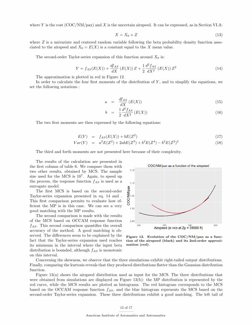
We follow the same method as described above. The screening is realized and the evolution of the cost withrespect to the airspeed variability is presented with the black curve in Figure 12. The cost increases whenthe airspeed increases. This is related to the effect of the Mach number on the aerodynamic efficiency of theairplane and more precisely the compressibility effects. When speed reduces, the cost finds a minimum beforeincreasing again. This is related to the existence of an optimum speed for each altitude. Since this curveis not linear, we rely on a second-order Taylor-series expansion to propagate the moments of the airspeeduncertainty beta distribution.

Let fAS be the function shown on Figure 12 (black):

fAS : IR → IR

X 7→ Y = fAS(X)(12)

11 of 17


where Y is the cost (COC/NM/pax) and X is the uncertain airspeed. It can be expressed, as in Section VI.A:

X = X0 + Z (13)

where Z is a univariate and centered random variable following the beta probability density function asso-ciated to the airspeed and X0 = E(X) is a constant equal to the X mean value.

The second-order Taylor-series expansion of this function around X0 is:

Y = fAS(E(X)) +dfASdX

(E(X))Z +1

2

d2fASdX2

(E(X))Z2 (14)

The approximation is plotted in red in Figure 12.In order to calculate the four first moments of the distribution of Y , and to simplify the equations, we

set the following notations :

a =dfASdX

(E(X)) (15)

b =1

2

d2fASdX2

(E(X)) (16)

The two first moments are then expressed by the following equations:

E(Y ) = fAS(E(X)) + bE(Z2) (17)

V ar(Y ) = a2E(Z2) + 2abE(Z3) + b2E(Z4)− b2E(Z2)2 (18)

The third and forth moments are not presented here because of their complexity.

Figure 12. Evolution of the COC/NM/pax as a func-tion of the airspeed (black) and its 2nd-order approxi-mation (red).

The results of the calculation are presented inthe first column of table 6. We compare them withtwo other results, obtained by MCS. The samplesize used for the MCS is 107. Again, to speed upthe process, the response function fAS is used as asurrogate model.

The first MCS is based on the second-orderTaylor-series expansion presented in eq. 14 and .This first comparison permits to evaluate how ef-ficient the MP is in this case. We can see a verygood matching with the MP results.

The second comparison is made with the resultsof the MCS based on OCCAM response functionfAS . This second comparison quantifies the overallaccuracy of the method. A good matching is ob-served. The differences seem to be explained by thefact that the Taylor-series expansion used reachesits minimum in the interval where the input betadistribution is bounded, although fAS is monotonicon this interval.

Concerning the skewness, we observe that the three simulations exhibit right-tailed output distributions.Finally, comparing the kurtosis reveals that they produced distributions flatter than the Gaussian distributionfunction.

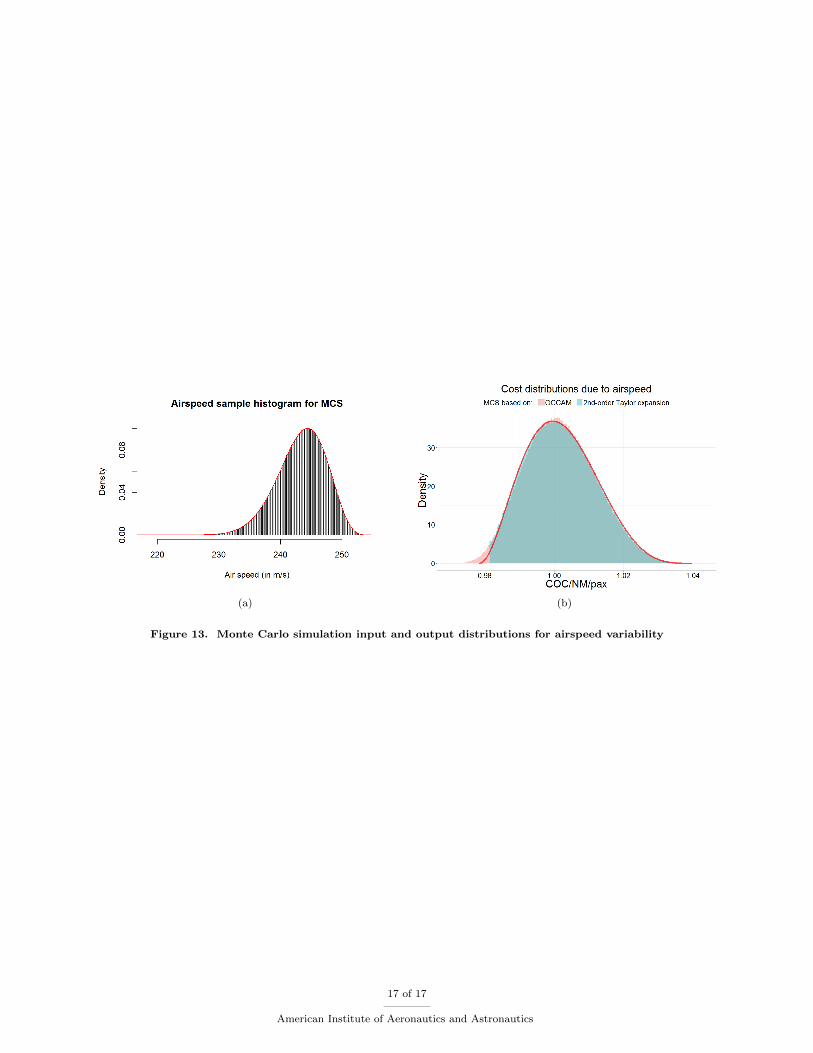
Figure 13(a) shows the airspeed distribution used as input for the MCS. The three distributions thatwere obtained from simulations are displayed on Figure 13(b): the MP distribution is represented by thered curve, while the MCS results are plotted as histograms. The red histogram corresponds to the MCSbased on the OCCAM response function fAS , and the blue histogram represents the MCS based on thesecond-order Taylor-series expansion. These three distributions exhibit a good matching. The left tail of

12 of 17


Table 6. First four moments of the beta distribution for the costs due to airspeed parameter.

Moments MP MCS withTaylor*

Relativedifference

MCS withOCCAM+

Relativedifference

E(Y ) 1.0020 1.0019 -0.01 % 1.0018 -0.02 %

V ar(Y ) 1.0086e-5 1.0090e-05 0.05 % 1.0466e-05 -3.63 %

Third centered moment 2.928e-07 2.934e-07 0.23 % 2.381e-07 23.0 %

Forth centered moment 2.605e-08 2.607e-08 0.07 % 2.996e-08 -13.1 %

Skewness 0.289 0.289 N/A 0.222 N/A

Kurtosis 2.561 2.560 N/A 2.736 N/A

* MCS realized using the second-order Taylor-serie expansion presented in eq. 14.+ MCS realized using the OCCAM model.

the blue distribution is cut. This is due to the fact that the Taylor expansion reaches its minimum in theinterval where the airspeed distribution is bounded.

This sub-section has shown that MP techniques are very efficient for determining the cost distributionarising from airspeed variability. We have compared MP results with those produced using two MCS strate-gies, one relying on the actual OCCAM response function, and the other one based on the second-orderTaylor-series expansion. In both case, differences appear to be negligible.

VII. Conclusion

The aim of this paper was to model airplane operational parameter uncertainties in order to quantifythe resulting uncertainty in the estimation of the cost of the mission. The four flight parameters consideredwere the air range, the average cruise altitude, the average cruise speed and the average difference betweenthe air temperature in cruise and the ISA temperature at the same altitude. The cost observed was the cashoperating cost per nautical mile per passenger. The data were extracted from the MOZAIC database. Wethen focused our analysis on four particular airplanes of one specific long-range type. The model chosen forbuilding the associated statistical distribution was a beta distribution. It proved to be efficient to modelairspeed and temperature distributions but not for air range and cruise speed. We therefore focused on thesefirst two parameters and propagated them to identify the related distribution of operational costs. A first-order Taylor-series expansion combined with the moment propagation technique was used for the temperatureand yield good results. A second-order Taylor-series expansion together with moment propagation was usedfor the airspeed and the results validated the method used.

Concerning the impact on cost, we showed in the preliminary analysis that the effect of air range could behigh. For airspeed and temperature, the variability observed is much smaller and of one order of magnitudeof few percents.

In this work, we have used a tool dedicated to overall airplane preliminary design, and the propagationof the studied uncertainties can be propagated and later used for robust design optimization in order tomeet better the needs of the airlines and the passengers, and to limit the human impact on the environmentthrough more efficient design and operation interconnections.

Further work is now anticipated to push the limit of the presented analysis. First, in this paper, only theaverage values during cruise were considered for altitude, speed and temperature, although much more datais available from the database. Also, these parameters have been considered to be independent althoughinter-correlations between them probably exist. Payload is another important parameter that has not beenincluded in our analysis because it was not available. We also limited our study to beta distributions forrepresenting the operational variabilities. Other statistical models should be considered to grasp furthermoreinformation from the data available. We limited the study to the costs but it could be broaden to otherparameters of interest (mass, etc.).

13 of 17


Acknowledgments

The authors acknowledge the strong support of the European Commission, Airbus, and the Airlines(Lufthansa, Air-France, Austrian, Air Namibia, Cathay Pacific, Iberia and China Airlines so far) who carrythe MOZAIC or IAGOS equipment and perform the maintenance since 1994. MOZAIC is presently fundedby INSU-CNRS (France), Meteo-France, Universite Paul Sabatier (Toulouse, France) and Research CenterJulich (FZJ, Julich, Germany). IAGOS has been and is additionally funded by the EU projects IAGOS-DSand IAGOS-ERI. The MOZAIC-IAGOS database is supported by ETHER (CNES and INSU-CNRS). Dataare also available via Ether web site http://www.pole-ether.fr

References

1ACARE, “Strategic Research and Innovation Agenda,” http://www.acare4europe.com/sria, 2012, Advisory Council forAviation Research and innovation in Europe.

2OAG, “OAG Analyser/Schedules Analyser,” http://analytics.oag.com, 2015, OAG Aviation Worldwide Ltd.3IAGOS, “MOZAIC IAGOS Database,” http://www.iagos.org/, 2016, European Research Infrastructure IAGOS (In-service

Aircraft of a Global Observing System).4Birman, J., Uncertainty quantification and propagation in Conceptual Aircraft Design: From deterministic optimization

to chance constrained optimization, Ph.D. thesis, Universite de Toulouse III - Paul Sabatier, Toulouse, France, 2013.5Prigent, S., Innovative and integrated approach for environmentally efficient aircraft design and operations, Ph.D. thesis,

ISAE-Supaero, Toulouse, France, 2015.6“Scilab,” http://www.scilab.org/, 2016, Scilab Enterprises S.A.S.7Lambe, A. B. and Martins, J. R. R. A., “Extensions to the design structure matrix for the description of multidisciplinary

design, analysis, and optimization processes,” Structural and Multidisciplinary Optimization, Vol. 46, No. 2, 2012, pp. 273–284.

14 of 17


MTOW

(0)

MZFW

(0)

1:

MDA

2:TLAR

3:TLAR

4:TLAR

5:TLAR

5.1:TLAR

5.2

:TLAR

7:TLAR

8:TLAR

2:

Airfram

eGeometry

4:

Airfram

eCom

pon

ents

Geometry

Fuel

Tan

kVolume

7:Airfram

eCompon

ents

Geometry

MTOW

MZFW

3,6→

4:

MassMission

Loop

4:DesignMTOW

DesignMZFW

5:FuelBlock

MTOW

7:MLW

MTOW

8:Airfram

eCom

pon

ents

Masses

MTOW

MW

E

6:MTOW

Nom

inalPayload

Max

Payload

OW

E

4:

Masses

6:FuelTotal

Ran

geZFW

5:

Mission

5.1:MassRef

Cruise

5.2:MassR

efCruise

5.3

:LoD

5.1

:HighSpeed

Aerodynam

ics

5.2:LoD

5.3:TSFC

Cruise

5.2:

Propulsion

9:AirplaneOperational

Perform

ances

7:

Perform

ances

9:COC

DOC

RC

8:

Costs

Figure 8. Multidisciplinary Design Analysis Process used for the propagation of the uncertainties

15 of 17


Figure 9. 3-view drawing of the reference airplane.

(a) (b)

Figure 11. Monte Carlo simulation input and output distributions for delta ISA temperature variability

16 of 17


(a) (b)

Figure 13. Monte Carlo simulation input and output distributions for airspeed variability

17 of 17


modeling operational variability for robust

Documents