measurements and simulations of the near-surface ...solgel/publicationspdf/2009/... · measurements...
TRANSCRIPT

Measurements and simulations of the near-surface composition
of evaporating ethanol–water droplets
Christopher J. Homer,a Xingmao Jiang,b Timothy L. Ward,c C. Jeffrey Brinkerbcd
and Jonathan P. Reid*a
Received 26th February 2009, Accepted 7th May 2009
First published as an Advance Article on the web 3rd June 2009
DOI: 10.1039/b904070f
The evolving composition of evaporating ethanol–water droplets (initially 32.6 or 45.3 mm radius)
is probed by stimulated Raman scattering over the period 0.2 to 3 ms following droplet
generation and with a surrounding nitrogen gas pressure in the range 10 to 100 kPa. The
dependence of the evaporation rate on the relative humidity of the surrounding gas phase is also
reported. The measured data are compared with both a quasi-steady state model and with
numerical simulations of the evaporation process. Results from the numerical simulations are
shown to agree closely with the measurements when the stimulated signal is assumed to arise
from an outer shell with a probe depth of 2.9 � 0.4% of the droplet radius, consistent with a
previous determination. Further, the time-dependent measurements are shown to be sensitive to
the development of concentration gradients within evaporating droplets. This represents the first
direct measurement of the spatial gradients in composition that arise during the evaporation of
aerosol droplets and allows the influence of liquid phase diffusion within the condensed phase on
droplet evaporation to be examined.
I. Introduction
It is important to understand the mass and heat transfer
occurring during the growth or evaporation of liquid aerosol
droplets when studying the rapid evaporation processes that
occur during the delivery of fuels for combustion, the delivery
of drugs to the lungs and during spray drying.1–5 The rapid
evaporation of volatile components can lead to substantial
changes in droplet surface temperature, thereby influencing
the mass transfer rate.6 Significant gradients in composition
can be established in the condensed phase as the droplet
evaporates if the rate of liquid phase diffusion is slow
compared to the rate of mass transfer to the surrounding
vapour.1 The evaporation dynamics are unsteady and the
coupled mass and energy conservation equations must be
solved simultaneously.7–9
Numerous experimental techniques have been applied to
study the rates of mass and heat transfer of growing or
evaporating aerosol. Many of the measurements on individual
isolated droplets have been made with electrostatic, acoustic
or optical traps, and have focused on the determination of
component vapour pressures through measurements of the
slow evaporation of low volatility organic components.10–13
The droplet size has been commonly determined by elastic
light scattering or evolving mass. Under these conditions, the
evaporation process can be assumed to proceed isothermally
and the mass and heat transfer can be decoupled. There are
few examples of the direct characterisation of the unsteady
evaporation of aerosol droplets.6–9,14 Elastic light scattering
has been applied to probe evolving particle size and refractive
index. However, there have been very few direct measurements
of evolving particle composition.15–18
We have shown that the non-linear stimulated Raman
signature from evaporating mixed component droplets,
referred to below as cavity enhanced Raman scattering
(CERS), can be used to characterise the evolving composition
of evaporating alcohol/water droplets.15,16 By combining
pulsed laser illumination with a droplet train instrument, the
depletion in concentration of the more volatile alcohol
component can be determined with variation in surrounding
gas pressure over time frames from 0.2 to 10 ms. The
amplification of the Raman signal occurs at wavelengths
commensurate with whispering gallery modes (WGMs) and
the signal intensity from a particular component scales
exponentially with concentration. Thus, CERS provides a
highly sensitive signature of composition: the composition of
ethanol–water solution droplets can be determined with an
accuracy of �0.2% v/v over the compositional range 16 to
19% v/v ethanol in water, where % v/v refers to the percentage
by volume of the alcohol prior to mixing, with balance of
water. We have used this technique to measure the depletion of
methanol, ethanol or propanol from mixed alcohol/water
droplets,15,16 initially in the radius range 20–60 mm, at
surrounding dry nitrogen gas pressures in the range 10 to
100 kPa.
In our previous work, the experimental measurements at a
fixed and early evaporation time of 0.2 ms were compared to a
a School of Chemistry, University of Bristol, Bristol, UK BS8 1TSbCenter for Micro-Engineered Materials, University of New Mexico,Albuquerque, NM 87106, USA
cDepartments of Chemical and Nuclear Engineering and MolecularGenetics and Microbiology, University of New Mexico, Albuquerque,NM 87106, USA
dSandia National Laboratories, Albuquerque, NM 87106, USA
7780 | Phys. Chem. Chem. Phys., 2009, 11, 7780–7791 This journal is �c the Owner Societies 2009
PAPER www.rsc.org/pccp | Physical Chemistry Chemical Physics
quasi-steady model (QSS), initially presented by Newbold and
Amundsen.19 This approach assumes that at any particular
instant in time the concentration and temperature profiles in
the surrounding gas-phase can be represented by a steady state
profile.20,21 Changes in temperature or concentration profile
are accompanied by a change in the boundary conditions at
the droplet surface. This is a good approximation if the
timescale for adopting a stable temperature and concentration
profile in the gas phase is short compared to the timescale over
which the boundary conditions are changing.20
A major failing of the QSS model used in our previous work
is that it does not account for the developing concentration
and temperature gradients that are established within the
droplet. For example, the initial more rapid loss of the volatile
alcohol component than the aqueous component from the
droplet surface leads to surface depletion of the alcohol while
the droplet bulk remains at the initial composition.16,22 When
accompanied by the temperature depression at the surface, it is
anticipated that the mass flux of the alcohol from the surface
should decrease over time.23 Given that the non-linear Raman
signal provides a measure of the composition in the outer shell
of the droplet, the failure of the QSS model to represent the
evaporation dynamics with increasing time or increasing mass
flux of alcohol from the droplet is to be expected.
In this publication we present new measurements of the
evolving composition of ethanol–water droplets, extending
our previous measurements to times longer than 0.2 ms and
up to 3 ms over a range of gas pressures from 10 to 100 kPa.
The failure of the QSS model to represent the evaporation
process is illustrated over this extended range of conditions.
A numerical simulation of droplet evaporation is presented
and compared to the experimental observations, demonstrating
that the measurements are able to characterise the developing
concentration gradients near the droplet surface during
evaporation.
II. Theoretical representations of droplet
evaporation
Two models have been used to simulate the experimental
measurements of the depletion of ethanol with change in gas
pressure and with evolving time. The first model is the QSS
model, initially presented by Newbold and Amundsen.19 This
has been discussed at length in previous publications.16,23 The
second method, based on numerical simulation, is discussed in
this publication.
II.a The quasi-steady state model
In previous publications, we have used the QSS model to
simulate the composition and temperature of binary droplets
containing alcohol and water of different initial radii at an
evaporation time of 0.2 ms and at surrounding gas pressures in
the range 10–100 kPa.16,23 Systems studied have included the
evaporation of binary droplets of methanol–water, ethanol–
water and 1-propanol/water, and the ternary system
methanol–ethanol/water.16,22,23
A number of assumptions are inherent to the QSS
treatment.16,19 Firstly, the composition of the gas phase at
the liquid surface is assumed to be governed by equilibrium
thermodynamics, with a composition determined by the
liquid phase composition and temperature at the surface.
The effect of surface tension on vapour pressure is assumed
to be negligible and is ignored. Further, the profiles of
temperature and composition surrounding the droplet
can be approximated to steady-state profiles at any instant
in time. Finally, it is assumed that mass and heat transfer
within the droplet are instantaneous compared to transfer
within the gas phase and, as a consequence, the temperature
and composition remain uniform throughout the entire
droplet volume.
The assumption of spatial uniformity in composition during
evaporation must be contrasted with the origin of the CERS
signal, which is sensitive only to the composition near the
droplet surface, rather than the whole droplet bulk. Thus, the
CERS signal is expected to provide a measure of the alcohol
depletion in the outer shell of the droplet to a maximum probe
depth of B25% of the droplet radius.24 Indeed, our previous
work has suggested that the signal arises from a much
narrower volume element with shorter penetration depth from
the surface: the signal is non-linear and double resonance in
origin and, thus, more spatially confined than the penetration
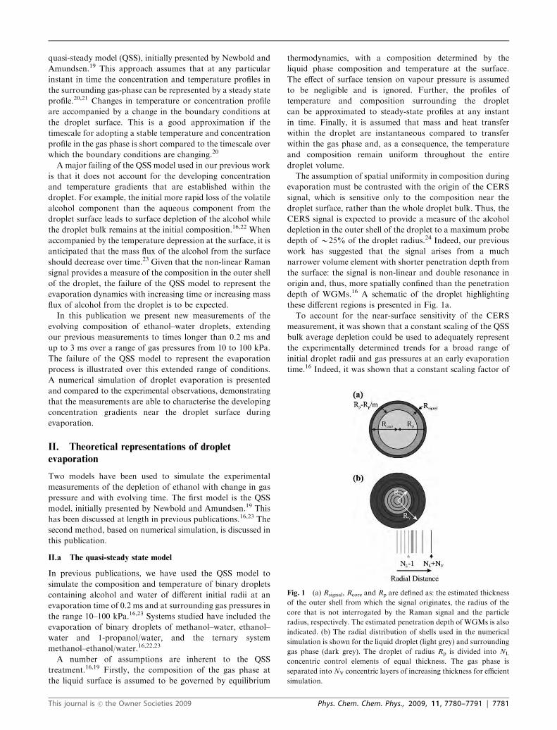
depth of WGMs.16 A schematic of the droplet highlighting
these different regions is presented in Fig. 1a.
To account for the near-surface sensitivity of the CERS
measurement, it was shown that a constant scaling of the QSS
bulk average depletion could be used to adequately represent
the experimentally determined trends for a broad range of
initial droplet radii and gas pressures at an early evaporation
time.16 Indeed, it was shown that a constant scaling factor of
Fig. 1 (a) Rsignal, Rcore and Rp are defined as: the estimated thickness
of the outer shell from which the signal originates, the radius of the
core that is not interrogated by the Raman signal and the particle
radius, respectively. The estimated penetration depth of WGMs is also
indicated. (b) The radial distribution of shells used in the numerical
simulation is shown for the liquid droplet (light grey) and surrounding
gas phase (dark grey). The droplet of radius Rp is divided into NL
concentric control elements of equal thickness. The gas phase is
separated into NV concentric layers of increasing thickness for efficient
simulation.
This journal is �c the Owner Societies 2009 Phys. Chem. Chem. Phys., 2009, 11, 7780–7791 | 7781
11.4 � 3.0 could be used to represent all of the binary systems
studied, methanol–water, ethanol–water and 1-propanol–
water, at an evaporation time of 0.2 ms. This scaling factor
was shown to be equivalent to assuming that the probe depth
of the CERS signal was only B3% of the droplet radius,
typically 1 mm for the droplet sizes studied.
The use of a single scaling factor to represent all of the
alcohol/water systems studied by the QSS model can be
attributed to two key factors. Firstly, the refractive indices
of all binary and ternary solutions studied are similar, with the
consequence that the optical probe depth is expected to be
similar for all three systems.16,25 Secondly, the liquid phase
diffusion coefficients for all alcohol components are similar in
magnitude. When considered in conjunction with the
early evaporation times studied (B0.2 ms for all systems),
the gradient in composition arising from surface depletion
is expected to be established over a much shorter length
scale than the probe depth. Thus, it is anticipated that the
QSS representation of the experimental data should
deteriorate at longer fall times, higher depletions of alcohol
and for smaller droplets, and that the required scaling factor is
not a constant. This is in addition to the clear failings of the
QSS model to reflect the details of the dynamic processes
occurring.
II.b Numerical simulation of the moving boundary problem
A second, more appropriate numerical simulation is now
presented as an alternative to the QSS model to simulate the
evaporation of binary alcohol/water droplets.26 The physical
properties of an evaporating droplet are interconnected and
change nonlinearly with time. The droplet boundary is also
changing with time as the droplet grows or evaporates. This
leads to a one-dimensional time-dependent moving boundary
Stefan problem. Mathematical analysis of this moving boundary
problem is complex, and much research has been conducted to
find a solution to this problem. Fixed27 and variable28–30
time-step methods have been developed to examine the
problem with implicit boundary conditions; these methods
are discussed and compared in detail by Moyano and
Scarpettini.31 Further attempts to solve the problem have also
been proposed by Rizwan-Uddin,32 Asaithambi33 and
Caldwell et al.34
The numerical simulation presented here circumvents the
difficulty of solving the moving boundary problem by
converting it to a fixed boundary problem by assuming that
the boundary does not move over a small time step. A full
description of the simulation method will be presented by
Jiang and Brinker in a subsequent paper and details are
presented in ref. 26. The purpose of this publication is to
compare the numerical simulations with the experimental data
and only a brief description of the model will be
presented here.
The droplet and its surrounding vapour phase are divided
into a large number of concentric segments (Fig. 1b),
respectively NL and NV. For computational efficiency, the
initial volume elements are designed with varying size and
are chosen to be most dense for the regions near the droplet
surface where gradients in concentration and temperature are
steep. The control volumes near the surface may be merged
with a neighbouring layer of the same phase or divided
into two layers to keep the grid spacing small and enable
convergence, accuracy and quick numerical simulation. For
modelling the evaporation of a droplet into an ‘infinite’
volume of air, the vapour phase grid spacings are chosen to
take a power relationship to reduce NV and increase the
efficiency of simulation without compromising the accuracy.
The Stefan problem is then treated as an integration of a series
of small consecutive changes as the physical properties of the
droplet change with time, t - t + dt. This allows the
calculation of mass and heat transfer for a droplet with a
fixed boundary; the new boundary is determined after each
time step and the calculation repeated. When performed with a
series of small time steps and with a small enough grid size, the
calculations approximate closely to the solution that would be
achieved if the problem were treated as a moving boundary
problem.
More specifically, the evaporation dynamics characterised
in the experiments can be treated within the continuum regime
and are controlled by gas phase diffusion. As in the QSS
model, the vapour and liquid phases at the droplet surface are
assumed to remain at equilibrium. For a spherical stationary
system without chemical reaction, the mass transport of this
isotropic diffusion system can be described by a continuity
equation for species i:
@Ci
@t¼ 1
r2@
@rr2Di
@Ci
@r
� �ð1Þ
where Ci is the concentration of component i, t is the
evaporation time, Di is the diffusion coefficient of component
i and r is the radial distance. Similarly, the heat transport can
be described as
rCP@T
@t¼ 1
r2@
@rr2k
@T
@r
� �ð2Þ
where r is the density of the solution or gas phase, CP is heat
capacity of the solution or gas phase and T is the temperature.
Eqn (1) and (2) are valid only for evaporation without radial
convection. This is a reasonable approximation for droplets
with negligible internal pressure gradient and for which
concentration and temperature gradients result in mass and
thermal diffusion alone. These partial differential equations
are difficult to solve simultaneously as all physical properties
are interconnected and change with time and location. In
addition, the droplet size changes with time.
To solve the coupled mass and heat transport problem, the
moving boundary problem can be solved explicitly as an
integration of a series of consecutive conventional fixed-
boundary heat-transport-only, mass-transport-only, and
control volume shrinkage/expansion-only steps.26 The
time step can be fixed at a low value (10�6 s) or increased
gradually with developing temperature and concentration
profiles to reduce computational time while ensuring
convergence of the simulation.26 Eqn (1) and (2) are solved
by a finite difference method subject to the following initial
and boundary conditions. Considering an initial concen-
tration distribution that is uniform throughout the droplet,
7782 | Phys. Chem. Chem. Phys., 2009, 11, 7780–7791 This journal is �c the Owner Societies 2009
the initial and boundary conditions for component i are given
as follows:
Ci(r,0) = Ci,0 for 0 r r r RNL,0 (3)
Ci(r,0) = Ci,0,V for RNL,0 o r r RNL+NV,0 (4)
@Ci
@r
� �����r¼0¼ 0 ð5Þ
@Ci
@r
� �����RNLþNV
¼ 0 or Ci ¼ Ci;1 at RNLþNV ¼ 1 ð6Þ
RNL and RNL+NV are droplet radius and the radius of outer-
most vapor layer. A subscript of 0 denotes t = 0 s, or the initial
state. The mass balance for component i in the liquid layer (NL)
at the interface during time t and t + dt can be written as:
R2NL�1ðRNL � RNL�1Þ
Ci;NLðtþ dtÞ � Ci;NLðtÞdt
¼ 2R2NLD
Vi;NL
Ci;NLþ1ðtÞ � Ci;NL;eqðtÞRNLþ1 � RNL
� R2NL�1Di;NL�1
Ci;NLðtÞ � Ci;NL�1ðtÞRNL � RNL�1
ð7Þ
where theDVi,NL refers to the diffusion coefficient of i in the first
vapour layer, and Ci,NL,eq is the vapor phase concentration at
equilibrium with liquid compositions for the liquid layer, NL.
For the first vapour element, the mass balance is:
R2NLðRNLþ1 � RNLÞ
Ci;NLþ1ðtþ dtÞ � Ci;NLþ1ðtÞdt
¼ R2NLþ1Di;NLþ1
Ci;NLþ2ðtÞ � Ci;NLþ1ðtÞRNLþ2 � RNLþ1
� 2R2NLD
Vi;NL
Ci;NLþ1ðtÞ � Ci;NL;eqðtÞRNLþ1 � RNL
ð8Þ
Correspondingly, the initial and boundary conditions for heat
transport can be defined in a similar way as:
T(r,0) = T0,L for 0 r r r RNL,0 (9)
T(r,0) = T0,V for RNL,0 o r r RNL+NV,0 (10)
@T
@r
� �����r¼0¼ 0 ð11Þ
@T
@r
� �����RNLþNV
¼ 0 or T ¼ T1 at RNLþNV ¼1 ð12Þ
The heat balance for the outer liquid layer (NL) can be written
as the following equation:
R2NL�1ðRNL � RNL�1ÞrNLCPNL
TNLðtþ dtÞ � TNLðtÞdt
¼ 2R2NLk
VNL
TNL þ 1ðtÞ � TNLðtÞRNLþ1 � RNL
þ 2R2NL
Xi
DVi;NL
Ci;NLþ1ðtÞ � Ci;NL;eqðtÞRNLþ1 � RNL
D �Hi;evp
� R2NL�1kNL�1
TNLðtÞ � TNL�1ðtÞRNL � RNL�1
ð13Þ
and for the first vapor element as:
R2NLðRNLþ1 � RNLÞrNLþ1CPNL þ 1
TNL þ 1ðtþ dtÞ � TNL þ 1ðtÞdt
¼ R2NLþ1kNLþ1
TNLþ2ðtÞ � TNLþ1ðtÞRNLþ2 � RNLþ1
� 2R2NLk
VNL
TNLþ1ðtÞ � TNLðtÞRNLþ1 � RNL
ð14Þ
where k is heat conduction coefficient and D �Hi is the partial
molar evaporation heat for component i. The solubility of air
or nitrogen in the droplets is neglected.
Adjustment of the control volumes is achieved by self-
attuning based on mass balance and pressure conservation
following the updated temperature and concentrations.
Primed and unprimed quantities refer to the property after
or before the time increment, respectively. The volume
shrinkage/expansion coefficient, ZLj for liquid layer j over time
dt can be obtained by
ZLj ¼V 0jVj¼
43pðR 03j � R
03j�1Þ
43pðR3
j � R3j�1Þ¼
Pi
mwiC0iP
i
mwiCi� rr0
ð15Þ
where r is a function of composition and temperature, mwi is
the molecular weight for component i, and C0i, R0i, and r0 are
the updated concentration for component i at the updated
radius and updated density for jth element. Similarly, the
volume shrinkage/expansion coefficient, ZLj for vapor layer
j over time dt is given by
ZVj ¼V 0jVj¼
Pi
mwiC0iP
i
mwiCi� mw
mw0� T0
Tð16Þ
Where T and T0 are the temperatures, and mw and mw0 are the
average molecular weight at t and t + dt for the jth vapour
layer. The volume updating starts first from the element at
droplet center and gradually extends outward to the liquid
layer near droplet interface and then to vapor layers while
keeping a fixed total gas pressure.
The initial conditions are used to update C and T and,
therefore, all other transient thermodynamic and transport
properties by mass balance (eqn (1)) and thermal balance
(eqn (2)) for each layer (element, control volume) within the
vapour phase and liquid phase over a time period t = 0 - dt.The boundary conditions are coupled to the updating of the
properties for the liquid layer at the droplet centre and at the
outermost vapour layer throughout all the simulation.
Step-by-step, all thermodynamic and transport properties for
each element can be calculated and updated over the
evaporation time. A discussion of the methods for describing
the solution thermodynamics and the thermophysical
properties required for these simulations is presented in
Appendix A.
II.c Numerical simulations of internal gradients in composition
With the QSS model, the total ethanol depletion is estimated
from the whole of the droplet volume; there is no
This journal is �c the Owner Societies 2009 Phys. Chem. Chem. Phys., 2009, 11, 7780–7791 | 7783
consideration of the developing spatial inhomogeneities in
composition at different radial depths within the droplet.
In contrast, the numerical simulations explicitly include
information on the heat and mass transfer occurring with
the condensed phase by resolving the droplet into a number of
concentric layers. Thus, the ethanol depletion in each layer
can be estimated, providing a radial profile of ethanol
concentration throughout the droplet volume and allowing
treatment of the heat and mass transfer occurring in both the
liquid and gas phases.
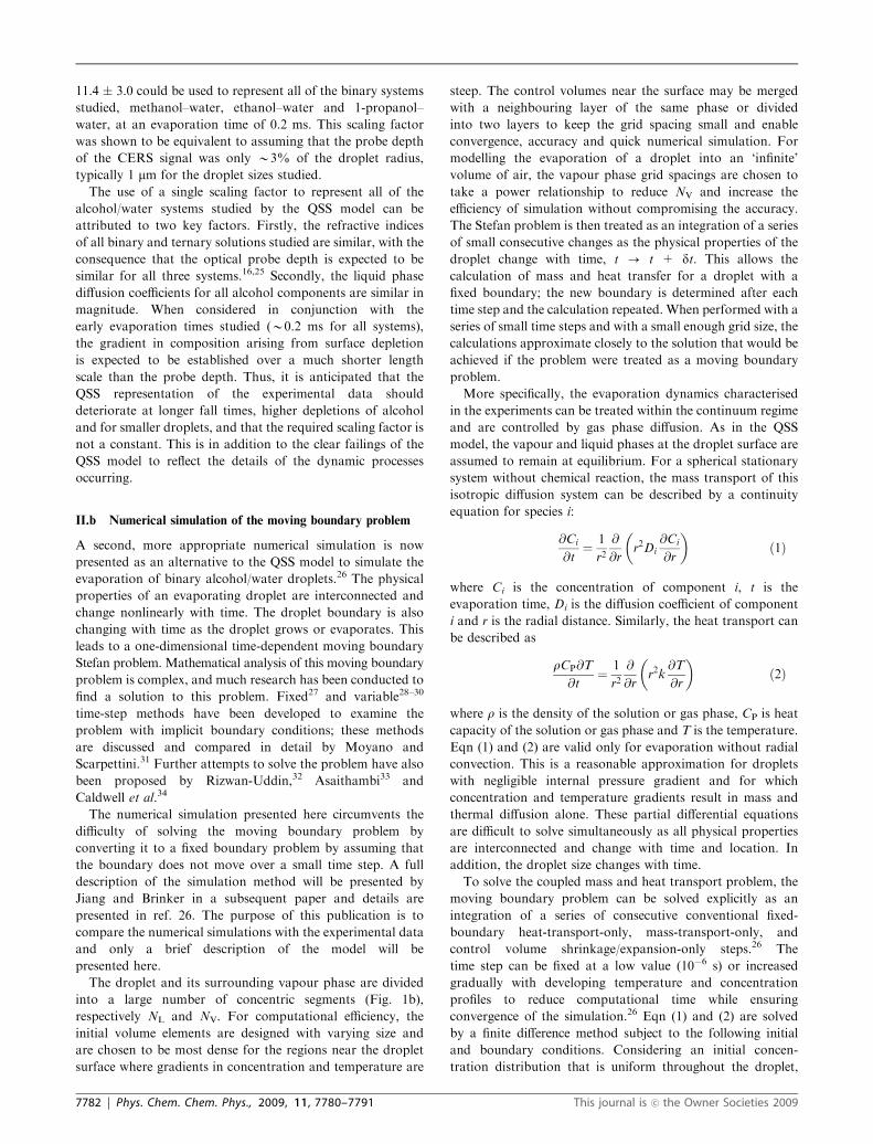
Fig. 2 illustrates the simulated radial concentration profile
of a single isolated droplet, initially 45.3 mm in radius and with
a composition of 18.4% v/v ethanol, resolved into 452 layers
of B100 nm thickness at an evaporation time of 0.5 ms.
Greater depletion occurs near the surface of the droplet,
establishing a concentration gradient that drives diffusion of
ethanol within the droplet from the bulk towards the surface.
The higher evaporative mass flux of ethanol from the droplet
at lower pressures (compare 100 and 10 kPa in Fig. 2) leads to
a more significant depletion of ethanol at the surface and a
larger concentration gradient within the droplet.
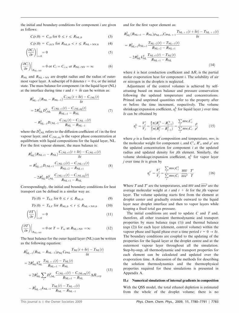
Fig. 3 presents the temporal evolution of the ethanol
depletion calculated at various depths from the droplet surface
at surrounding gas pressures in the experimental chamber of
10 kPa and 100 kPa. It can be seen that depletion is greater at a
fixed depth within the droplet when the surrounding gas
pressure is lower. Further, although ethanol is depleted in
concentration within the CERS probe volume (e.g. 250 nm)
from the very early times, the slow rate of liquid diffusion
ensures that the core of the droplet does not change in
composition until considerably later in time (e.g. compare
depths of 1 mm and 10 mm). This is the origin of the scaling
factor that must be introduced to allow comparison of the
estimated depletions from the QSS model and the experi-
mental measurements. Indeed, after B2 ms, the concentration
of ethanol at a depth of 250 nm begins to recover as liquid
diffusion replenishes the level of ethanol near the droplet
surface.
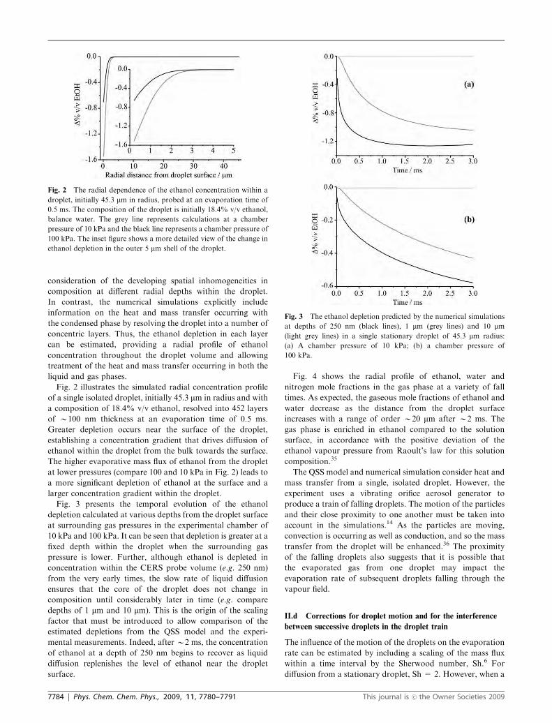
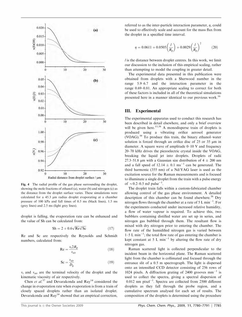
Fig. 4 shows the radial profile of ethanol, water and
nitrogen mole fractions in the gas phase at a variety of fall
times. As expected, the gaseous mole fractions of ethanol and
water decrease as the distance from the droplet surface
increases with a range of order B20 mm after B2 ms. The
gas phase is enriched in ethanol compared to the solution
surface, in accordance with the positive deviation of the
ethanol vapour pressure from Raoult’s law for this solution
composition.35
The QSS model and numerical simulation consider heat and
mass transfer from a single, isolated droplet. However, the
experiment uses a vibrating orifice aerosol generator to
produce a train of falling droplets. The motion of the particles
and their close proximity to one another must be taken into
account in the simulations.14 As the particles are moving,
convection is occurring as well as conduction, and so the mass
transfer from the droplet will be enhanced.36 The proximity
of the falling droplets also suggests that it is possible that
the evaporated gas from one droplet may impact the
evaporation rate of subsequent droplets falling through the
vapour field.
II.d Corrections for droplet motion and for the interference
between successive droplets in the droplet train
The influence of the motion of the droplets on the evaporation
rate can be estimated by including a scaling of the mass flux
within a time interval by the Sherwood number, Sh.6 For
diffusion from a stationary droplet, Sh = 2. However, when a
Fig. 2 The radial dependence of the ethanol concentration within a
droplet, initially 45.3 mm in radius, probed at an evaporation time of
0.5 ms. The composition of the droplet is initially 18.4% v/v ethanol,
balance water. The grey line represents calculations at a chamber
pressure of 10 kPa and the black line represents a chamber pressure of
100 kPa. The inset figure shows a more detailed view of the change in
ethanol depletion in the outer 5 mm shell of the droplet.
Fig. 3 The ethanol depletion predicted by the numerical simulations
at depths of 250 nm (black lines), 1 mm (grey lines) and 10 mm(light grey lines) in a single stationary droplet of 45.3 mm radius:
(a) A chamber pressure of 10 kPa; (b) a chamber pressure of
100 kPa.
7784 | Phys. Chem. Chem. Phys., 2009, 11, 7780–7791 This journal is �c the Owner Societies 2009
droplet is falling, the evaporation rate can be enhanced and
the value of Sh can be calculated from:
Sh ¼ 2þ 0:6ffiffiffiffiffiffiRep ffiffiffiffiffi
Sc3p
ð17Þ
Re and Sc are respectively the Reynolds and Schmidt
numbers, calculated from:
Re ¼ vt2Rp
vairð18Þ
Sc ¼ vair
Dgð19Þ
vt and vair are the terminal velocity of the droplet and the
kinematic viscosity of air respectively.
Chen et al.37 and Devarakonda and Ray14 considered the
change in evaporation rate when evaporation is from a train of
closely spaced droplets rather than an isolated droplet.
Devarakonda and Ray14 showed that an empirical correction,
referred to as the inter-particle interaction parameter, Z, couldbe used to effectively scale and account for the mass flux from
the droplet in a specified time interval.
Z ¼ 0:0611þ 0:0505l
Rp
� �þ 0:0029
l
Rp
� �2
ð20Þ
l is the distance between droplet centres. In this work, we limit
our discussion to the inclusion of this empirical scaling, rather
than attempting to model the coupling in greater detail.
The experimental data presented in this publication were
obtained from droplets with a Sherwood number in the
range 5.9–6.7 and the interaction parameter in the
range 0.69–0.81. An appropriate scaling to correct for both
of these factors is included in all of the theoretical simulations
presented here in a manner identical to our previous work.16
III. Experimental
The experimental apparatus used to conduct this research has
been described in detail elsewhere, and only a brief overview
will be given here.15,38 A monodisperse train of droplets is
produced using a vibrating orifice aerosol generator
(VOAG).39 To produce this train, the binary ethanol–water
solution is forced through an orifice disc of 25 or 35 mm in
diameter. A square wave of amplitude 0–10 V and frequency
20–70 kHz drives the piezoelectric crystal inside the VOAG,
breaking the liquid jet into droplets. Droplets of radii
27.3–51.8 mm with a Gaussian size distribution of 4 � 200 nm
and a fall speed of 12.14 � 0.1 ms�1 can be generated. The
third harmonic (355 nm) of a Nd:YAG laser is used as the
excitation source for the Raman measurements and is focused
to illuminate a single droplet from the train with a pulse energy
of B0.2–0.5 mJ pulse�1.
The droplet train falls within a custom-fabricated chamber
allowing control of the gas phase environment. A detailed
description of this chamber can be found elsewhere.38 Dry
nitrogen flows through the chamber at a rate of 5 L min�1. For
the experiments conducted under increased relative humidity,
a flow of water vapour is required. To achieve this, two
bubblers containing distilled water are set up in series, and
nitrogen gas bubbled through them. The resultant flow is
mixed with dry nitrogen prior to entering the chamber. The
flow rate of the humidified nitrogen gas is varied between
1–5 L min�1; the total flow rate of gas entering the chamber is
kept constant at 5 L min�1 by altering the flow rate of dry
nitrogen gas.
Raman scattered light is collected perpendicular to the
incident beam in the horizontal plane. The Raman scattered
light from the chamber is collimated and focused through the
entrance slit of a 0.5 m spectrograph. The light is dispersed
onto an intensified CCD detector consisting of 256 rows of
1024 pixels. A diffraction grating of 2400 grooves mm�1 is
used to collect the spectra, giving a spectral dispersion of
0.012 nm pixel�1. Spectra are collected from 2500 different
droplets as they fall through the probe region, and a
cumulative spectrum analysed for each set of results. The
composition of the droplets is determined using the procedure
Fig. 4 The radial profile of the gas phase surrounding the droplet,
showing the mole fractions of ethanol (a), water (b) and nitrogen (c) as
the distance from the droplet surface varies. These simulations were
calculated for a 45.3 mm radius droplet evaporating at a chamber
pressure of 100 kPa and fall times of 0.5 ms (black lines), 1.5 ms
(grey lines) and 2.5 ms (light grey lines).
This journal is �c the Owner Societies 2009 Phys. Chem. Chem. Phys., 2009, 11, 7780–7791 | 7785

to analyse the non-linear Raman signature established in
previous work.15,16,40
IV. Results and discussion
The depletion of ethanol has been measured for binary
ethanol–water droplets of initial radii of 32.6 and 45.3 mmand composition 18.4% v/v ethanol at evaporation/fall times
between 0.3 and 3 ms and dry nitrogen gas pressures between
10 and 100 kPa. In these measurements it is essential to
remember that the signal arises from the outer shell of the
droplet, rather than the droplet bulk, providing a measure of
the near surface composition and depletion of ethanol.
Initially, ethanol evaporates more rapidly from the droplet
giving rise to a concentration gradient within the droplet. The
concentration gradient is accompanied by liquid diffusion
which acts to counteract the initial depletion of ethanol.
In addition, the cooling of the surface leads to unsteady
evaporation and a relative change in mass flux of the two
components. Thus, it is essential to consider the depth probed
by the Raman signal and how an appropriate average value
can be estimated from the spatially resolved numerically
simulated depletions for comparison to the experimental
observations.
IV.a Consideration of the probe depth
In order to obtain a spatially averaged value for the ethanol
depletion for comparison with the experiments, it is necessary
to take into account the compositional variation over the
depth to which the droplet is being probed and the radial
distribution of the light intensity41 circulating within WGMs
inside the droplet. More specifically, the calculated mole
fraction of ethanol in each shell, xd,EtOH, at a distance from
the centre of the droplet, d, must be weighted by a scaling
factor, WG,d.
xv,EtOH = xd,EtOH � WG,d (21)
The weightings of each shell volume are assumed to follow a
Gaussian distribution around a dominant shell that is set to
have the maximum weighting, the shell that is considered to
contain the highest light intensity. This is subsequently
referred to as the probe depth, although it should be
remembered that this only represents the shell with the
maximum weighting and light does penetrate to a greater
depth. The weight for each volume element is calculated from
WG;d ¼1
sffiffiffiffiffiffi2pp e�ðVlayer�mÞ2=2s2 ð22Þ
where m is the value of the volume element at the maximum
intensity of the Gaussian intensity distribution and s is chosen
such that the integrated intensity of the Gaussian weighting
distribution remains independent of the chosen probe depth
and is equal to unity. Further, the Gaussian weighting is
chosen such that it decays to o5% of the peak, effectively
zero weighting, at the boundary of the droplet. Thus, the
maximum amplitude of the Gaussian weighting function
decreases as deeper regions of the droplet are allowed to
contribute to the signal and the radial range of the weighting
extends further from the droplet surface. Although the light
intensity distribution circulating within the droplet is not
accurately known, it is considered that a Gaussian weighting
should best represent the origin of the CERS double resonance
signal.24,41
The volume element, Vlayer, of each concentric shell is
approximated by
Vlayer = 4pR2inner�dR (23)
where dR is the thickness of the shell and Rinner is the inner
radial coordinate at which the shell is located. To obtain the
weighted mole fraction of ethanol across the entire probe
volume, the sum of xv,EtOH is divided by the sum of the
Gaussian weighting elements.
xEtOH ¼P
xv;EtOHPWG;d
ð24Þ
Fig. 5 shows the prediction of the ethanol depletion that would
be recorded from the Raman measurement as the probe depth
of the laser is allowed to vary for a droplet, initially 45.3 mm in
radius and with a composition 18.4% per vol ethanol, at an
evaporation time of 0.5 ms and at a pressure of 10 kPa or
100 kPa. As the signal is allowed to originate from deeper into
the droplet, the depletion of ethanol that would be recorded
diminishes due to the spatial inhomogeneity in composition
that is established during evaporation.
IV.b Comparison with measurements of depletions at varying
gas pressure
Previous work using the experimental technique described
here has focused on probing droplets shortly after their
production, principally at an evaporation time of 0.2 ms.15,16
Emphasis was particularly placed on exploring the
evaporation rates of different droplet sizes and different
volatile components at a range of pressures. Little work has
been done to probe the evaporation of droplets on longer
timescales, or to assess the accuracy of the QSS model to
represent depletion at longer fall times. This paper will
compare the numerical simulation and QSS model with
experimental measurements of binary ethanol–water droplet
evaporation on timescales up to 3 ms.
Fig. 5 The simulated ethanol depletion that would be detected
with varying laser probe depth for a 45.3 mm radius droplet at an
evaporation time of 0.5 ms and chamber pressures of 10 kPa (grey line)
and 100 kPa (black line).
7786 | Phys. Chem. Chem. Phys., 2009, 11, 7780–7791 This journal is �c the Owner Societies 2009

In Fig. 6, we report measurements of the depletion of
ethanol from evaporating droplets as a function of the
surrounding gas pressure and at four evaporation times
between 0.3 and 2.1 ms. The droplets are initially 32.6 mm in
radius and start with a composition of 18.4% v/v ethanol. The
depletion of ethanol at the earliest two fall times increases with
decreasing pressure due to the enhanced mass flux of ethanol
from the droplet due to the increasing rate of gas diffusion.
This is consistent with the trends observed in our previous
papers.15,16 At the longest evaporation time of 2.1 ms the
depletion of ethanol does not show a dependence on gas
pressure within the error bars of the measurements. Indeed,
although the depletion of ethanol decreases steadily at the high
pressure limit over the four times shown, the depletion at
10 kPa appears to be less at the longest evaporation time than
at 100 kPa. This observation is more obvious when the time
dependence is considered explicitly, as shown in Fig. 7(a) and
(b). As anticipated in our earlier discussion of the QSS model,
the agreement between the QSS predictions and the experi-
mental data is poor, particularly at the longest fall time,
predicting greater ethanol depletion than is observed. In this
comparison, we have applied the scaling factor of 11.4
determined previously.15,16
The results of numerical simulations are also included in
Fig. 6 with predictions from probe depths centred around
0.9 mm shown. By considering the quality of the fit to all of the
experimental data, this probe depth provides the most
accurate description of the data. Not only is the depletion
captured at high pressures, but the apparent decrease in the
extent of the depletion at the lowest pressures and longest fall
times is predicted. Indeed, when compared with the QSS
model, the numerical simulations more accurately reflect the
time dependence of the depletion, even out to 42 ms, as
shown in Fig. 7. The sensitivity of the modelled depletion
to the probe depth is apparent from considering the
predictions from probe depths of 800 nm and 1000 nm. A
probe depth of 900 � 100 nm corresponds to the signal
originating from a depth between 2.4 and 3.1% of the droplet
radius (32.6 mm).
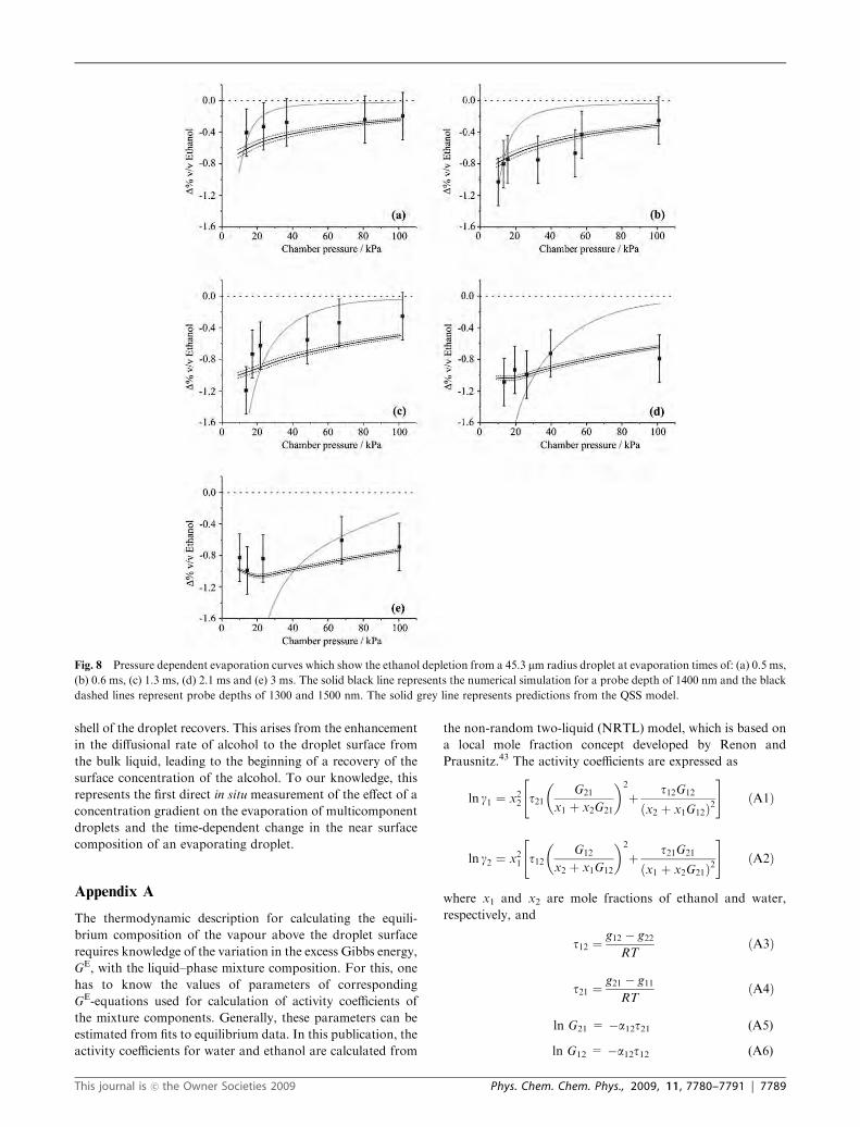
The evaporation of a droplet of initial radius 45.3 mm and
composition of 18.4% v/v ethanol has also been studied. Fig. 8
shows the pressure-dependent ethanol depletion measured at
evaporation times of 0.5, 0.6, 1.3, 2.1 and 3.0 ms. The QSS
model again predicts accurately the ethanol depletion on
sub-millisecond timescales, but is not successful in even
qualitatively capturing the trend recorded at evaporation
times of 1.3 ms and longer. Again, the data shows that the
ethanol depletion at early times and low pressures is marked,
but this does not continue as time progresses. Instead, the
pressure dependence becomes less pronounced and the time
dependence shows that the ethanol concentration appears to
recover with increasing time (Fig. 7(c)). The numerical simula-
tions again successfully capture the experimental trends for all
times and chamber pressures. Simulations from probe depths
of 1300, 1400 and 1500 nm are shown for comparison. This is
equivalent the signal arising from a probe depth between 2.9
and 3.3% of the initial droplet radius. Thus, the estimated
probe depths from both droplet sizes are consistent and
equivalent to 2.9 � 0.4% of the droplet radius. This is
consistent with our previous estimate of the probe depth
(3 � 1%) based on a comparison of the experimental data
with the QSS model but only at the earliest evaporation times.16
Fig. 6 Pressure dependent evaporation curves which show the ethanol depletion from a 32.6 mm radius droplet at evaporation times of: (a) 0.3 ms,
(b) 0.5 ms, (c) 1.3 ms and (d) 2.1 ms. The solid black line represents the numerical simulation for a probe depth of 900 nm and the black dashed
lines represent probe depths of 800 and 1000 nm. The solid grey line represents predictions from the QSS model.
This journal is �c the Owner Societies 2009 Phys. Chem. Chem. Phys., 2009, 11, 7780–7791 | 7787

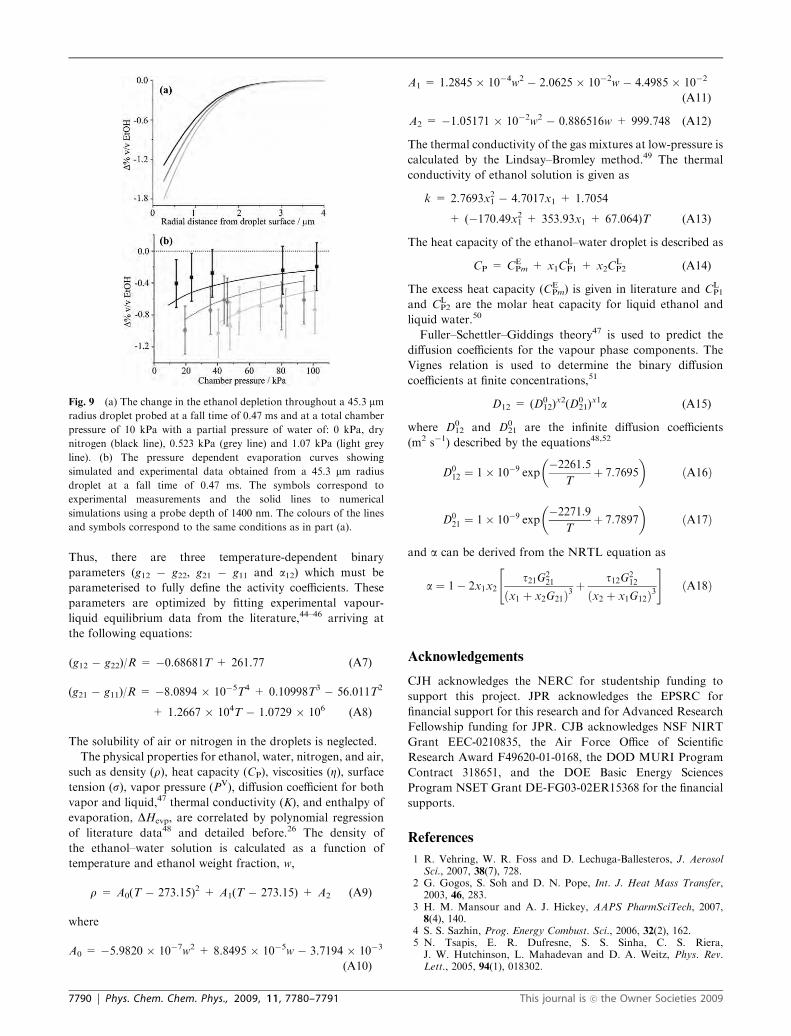
IV.c Evaporation measurements at varying relative humidity
The time-dependent ethanol concentration profile has been
simulated for a 45.3 mm droplet with varying relative humidity
of the gas phase varies. The saturation vapour pressure of
water calculated by the model has been altered to take into
account the addition of 0.52 and 1.1 kPa of water vapour to
the chamber, equivalent to relative humidities of 22 and 47%,
respectively, at 20 1C. This diminishes the vapour phase
concentration gradient of water between the droplet surface
and the infinite distance limit from the droplet, slowing the
mass flux of water. Fig. 9(a) shows the effect this has on the
predicted ethanol depletion throughout the droplet volume.
Increasing the relative humidity of the gas surrounding the
droplet increases the modelled ethanol depletion.
In experiments to compare with these predictions, nitrogen
gas was passed through two bubblers containing water before
being mixed with a dry nitrogen gas flow and then introduced
to the aerosol chamber. To measure the dependence of the
depletion on gas pressure, the mixing of dry and wet nitrogen
was controlled to maintain a constant partial pressure of water
in the chamber while changing the overall pressure. In
Fig. 9(b), the simulated and measured trends with varying
gas pressure and partial pressure of water are compared. It can
be seen that the numerical simulations predict, within the
experimental error, the extent to which ethanol depletion
increases when the relative humidity within the chamber is
increased.
V. Conclusions
The QSS model and the numerical simulations have been used
to model the evaporation of a binary ethanol–water droplet on
timescales up to 3 ms and the predictions are compared with
experimental measurements. The QSS model has been shown
to be only suitable for considering relative trends in the change
in concentration at a fixed evaporation time, requiring a
constant scaling factor to account for the spatial variation
and gradients in the droplet composition not accounted for by
the model.16 The QSS model fails to accurately capture the
experimental trends when the ethanol depletion is large at
millisecond and longer evaporation times or when the pressure
of the gas surrounding the droplet decreases. Forced
agreement between the QSS model and experiment would
require the introduction of a time dependent scaling factor,
which would indirectly account for the internal dynamics
occurring within the condensed phase but would hide the
details of the evaporation mechanism.
By contrast, the experimental measurements are found to be
consistent with the numerical simulations for all measure-
ments reported in this publication when the probe depth of
the stimulated Raman scattering signal is taken as 2.9 � 0.4%
of the droplet radius. This confirms that the experimental
measurements interrogate the spatial inhomogenieties in
composition that arise during evaporation. Specifically, the
outer shell of the droplet first exhibits a significant depletion in
the more volatile alcohol component, followed by a recovery
due to liquid phase diffusion; this behaviour is consistent with
the CERS measurement.
The probe depth is expected to depend only on refractive
index and should remain as a constant fraction of the droplet
size,B25% of the droplet radius for ethanol–water droplets.24
In this work, the probe depth is found to remain a constant
fraction of the size that is considerably less than what is
expected based on the penetration depth of the WGM. The
optical signal is non-linear in nature and follows an exponential
dependence on light intensity, leading to a narrower probe
depth than WGM penetration depth. Further, this must be
also coupled with the enhanced localisation of the signal due
to the double resonance nature of the probe, with signal at
highest gain arising from the volume of overlap between an
input WGM, one resonant with the laser wavelength, and an
output mode, one resonant with the Raman band contour.
These effects acting in combination lead to greater spatial
confinement in the signal when compared with the WGM
penetration depth, consistent with previous discussions.42
At longer times, the numerical simulations and experimental
trends agree that the concentration of the alcohol in the outer
Fig. 7 Comparison of the experimental trends (symbols) and theore-
tical predictions (QSS model, grey line; numerical simulations, black
lines) for the time dependence of the evaporation of (a) 32.6 mm radius
droplet at 100 kPa pressure; (b) 32.6 mm radius droplet at 10 kPa
pressure; (c) 45.3 mm radius droplet at 10 kPa pressure. The three
numerical simulations are for the probe depths reported in Fig. 6 and 8.
7788 | Phys. Chem. Chem. Phys., 2009, 11, 7780–7791 This journal is �c the Owner Societies 2009
shell of the droplet recovers. This arises from the enhancement
in the diffusional rate of alcohol to the droplet surface from
the bulk liquid, leading to the beginning of a recovery of the
surface concentration of the alcohol. To our knowledge, this
represents the first direct in situ measurement of the effect of a
concentration gradient on the evaporation of multicomponent
droplets and the time-dependent change in the near surface
composition of an evaporating droplet.
Appendix A
The thermodynamic description for calculating the equili-
brium composition of the vapour above the droplet surface
requires knowledge of the variation in the excess Gibbs energy,
GE, with the liquid–phase mixture composition. For this, one
has to know the values of parameters of corresponding
GE-equations used for calculation of activity coefficients of
the mixture components. Generally, these parameters can be
estimated from fits to equilibrium data. In this publication, the
activity coefficients for water and ethanol are calculated from
the non-random two-liquid (NRTL) model, which is based on
a local mole fraction concept developed by Renon and
Prausnitz.43 The activity coefficients are expressed as
ln g1 ¼ x22 t21G21
x1 þ x2G21
� �2
þ t12G12
ðx2 þ x1G12Þ2
" #ðA1Þ
ln g2 ¼ x21 t12G12
x2 þ x1G12
� �2
þ t21G21
ðx1 þ x2G21Þ2
" #ðA2Þ
where x1 and x2 are mole fractions of ethanol and water,
respectively, and
t12 ¼g12 � g22
RTðA3Þ
t21 ¼g21 � g11
RTðA4Þ
ln G21 = �a12t21 (A5)
ln G12 = �a12t12 (A6)
Fig. 8 Pressure dependent evaporation curves which show the ethanol depletion from a 45.3 mm radius droplet at evaporation times of: (a) 0.5 ms,
(b) 0.6 ms, (c) 1.3 ms, (d) 2.1 ms and (e) 3 ms. The solid black line represents the numerical simulation for a probe depth of 1400 nm and the black
dashed lines represent probe depths of 1300 and 1500 nm. The solid grey line represents predictions from the QSS model.
This journal is �c the Owner Societies 2009 Phys. Chem. Chem. Phys., 2009, 11, 7780–7791 | 7789
Thus, there are three temperature-dependent binary
parameters (g12 � g22, g21 � g11 and a12) which must be
parameterised to fully define the activity coefficients. These
parameters are optimized by fitting experimental vapour-
liquid equilibrium data from the literature,44–46 arriving at
the following equations:
(g12 � g22)/R = �0.68681T + 261.77 (A7)
(g21 � g11)/R = �8.0894 � 10�5T4 + 0.10998T3 � 56.011T2
+ 1.2667 � 104T � 1.0729 � 106 (A8)
The solubility of air or nitrogen in the droplets is neglected.
The physical properties for ethanol, water, nitrogen, and air,
such as density (r), heat capacity (CP), viscosities (Z), surfacetension (s), vapor pressure (PV), diffusion coefficient for both
vapor and liquid,47 thermal conductivity (K), and enthalpy of
evaporation, DHevp, are correlated by polynomial regression
of literature data48 and detailed before.26 The density of
the ethanol–water solution is calculated as a function of
temperature and ethanol weight fraction, w,
r = A0(T � 273.15)2 + A1(T � 273.15) + A2 (A9)
where
A0 = �5.9820 � 10�7w2 + 8.8495 � 10�5w � 3.7194 � 10�3
(A10)
A1 = 1.2845 � 10�4w2 � 2.0625 � 10�2w � 4.4985 � 10�2
(A11)
A2 = �1.05171 � 10�2w2 � 0.886516w + 999.748 (A12)
The thermal conductivity of the gas mixtures at low-pressure is
calculated by the Lindsay–Bromley method.49 The thermal
conductivity of ethanol solution is given as
k = 2.7693x21 � 4.7017x1 + 1.7054
+ (�170.49x21 + 353.93x1 + 67.064)T (A13)
The heat capacity of the ethanol–water droplet is described as
CP = CEPm + x1C
LP1 + x2C
LP2 (A14)
The excess heat capacity (CEPm) is given in literature and CL
P1
and CLP2 are the molar heat capacity for liquid ethanol and
liquid water.50
Fuller–Schettler–Giddings theory47 is used to predict the
diffusion coefficients for the vapour phase components. The
Vignes relation is used to determine the binary diffusion
coefficients at finite concentrations,51
D12 = (D012)
x2(D021)
x1a (A15)
where D012 and D0
21 are the infinite diffusion coefficients
(m2 s�1) described by the equations48,52
D012 ¼ 1� 10�9 exp
�2261:5T
þ 7:7695
� �ðA16Þ
D021 ¼ 1� 10�9 exp
�2271:9T
þ 7:7897
� �ðA17Þ
and a can be derived from the NRTL equation as
a ¼ 1� 2x1x2t21G2
21
ðx1 þ x2G21Þ3þ t12G2
12
ðx2 þ x1G12Þ3
" #ðA18Þ
Acknowledgements
CJH acknowledges the NERC for studentship funding to
support this project. JPR acknowledges the EPSRC for
financial support for this research and for Advanced Research
Fellowship funding for JPR. CJB acknowledges NSF NIRT
Grant EEC-0210835, the Air Force Office of Scientific
Research Award F49620-01-0168, the DOD MURI Program
Contract 318651, and the DOE Basic Energy Sciences
Program NSET Grant DE-FG03-02ER15368 for the financial
supports.
References
1 R. Vehring, W. R. Foss and D. Lechuga-Ballesteros, J. AerosolSci., 2007, 38(7), 728.
2 G. Gogos, S. Soh and D. N. Pope, Int. J. Heat Mass Transfer,2003, 46, 283.
3 H. M. Mansour and A. J. Hickey, AAPS PharmSciTech, 2007,8(4), 140.
4 S. S. Sazhin, Prog. Energy Combust. Sci., 2006, 32(2), 162.5 N. Tsapis, E. R. Dufresne, S. S. Sinha, C. S. Riera,J. W. Hutchinson, L. Mahadevan and D. A. Weitz, Phys. Rev.Lett., 2005, 94(1), 018302.
Fig. 9 (a) The change in the ethanol depletion throughout a 45.3 mmradius droplet probed at a fall time of 0.47 ms and at a total chamber
pressure of 10 kPa with a partial pressure of water of: 0 kPa, dry
nitrogen (black line), 0.523 kPa (grey line) and 1.07 kPa (light grey
line). (b) The pressure dependent evaporation curves showing
simulated and experimental data obtained from a 45.3 mm radius
droplet at a fall time of 0.47 ms. The symbols correspond to
experimental measurements and the solid lines to numerical
simulations using a probe depth of 1400 nm. The colours of the lines
and symbols correspond to the same conditions as in part (a).
7790 | Phys. Chem. Chem. Phys., 2009, 11, 7780–7791 This journal is �c the Owner Societies 2009
6 V. Devarakonda and A. K. Ray, J. Colloid Interface Sci., 2000,221, 104.
7 G. Castanet, A. Delconte, F. Lemoine, L. Mees and G. Grehan,Exp. Fluids, 2005, 39(2), 431.
8 G. Castanet, M. Lebouche and F. Lemoine, Int. J. Heat MassTransfer, 2005, 48(16), 3261.
9 A. K. Ray and S. Venkatraman, AIChE J., 1995, 41(4), 938.10 J. F. Widmann and E. J. Davis, Aerosol Sci. Technol., 1997, 27(2),
243.11 A. K. Ray, E. J. Davis and P. Ravindran, J. Chem. Phys., 1979,
71(2), 582.12 E. J. Davis and A. K. Ray, J. Chem. Phys., 1977, 67(2), 414.13 E. J. Davis, Aerosol Sci. Technol., 1997, 26(3), 212.14 V. Devarakonda and A. K. Ray, J. Aerosol Sci., 2003, 34(7), 837.15 R. J. Hopkins and J. P. Reid, J. Phys. Chem. A, 2005, 109, 7923.16 R. J. Hopkins and J. P. Reid, J. Phys. Chem. B, 2006, 110, 3239.17 G. Schweiger, J. Aerosol Sci., 1990, 21(4), 483.18 R. Vehring, H. Moritz, D. Niekamp, G. Schweiger and
P. Heinrich, Appl. Spectrosc., 1995, 49(9), 1215.19 F. R. Newbold and N. R. Amundson, AIChE J., 1973, 19(1), 22.20 T. Vesala, M. Kulmala, R. Rudolf, A. Vrtala and P. E. Wagner,
J. Aerosol Sci., 1997, 28(4), 565.21 J. Smolik and J. Vitovec, J. Aerosol Sci., 1984, 15(5), 545.22 C. R. Howle, C. J. Homer, R. J. Hopkins and J. P. Reid, Phys.
Chem. Chem. Phys., 2007, 9, 5344.23 R. J. Hopkins, C. R. Howle and J. P. Reid, Phys. Chem. Chem.
Phys., 2006, 8, 2879.24 R. Symes, R. M. Sayer and J. P. Reid, Phys. Chem. Chem. Phys.,
2004, 6, 474.25 Handbook of Chemistry and Physics, CRC Press LLC, 2006–2007.26 X. Jiang, Doctoral Thesis, The University of New Mexico, 2006.27 J. Ockendon and W. Hodgkins, Moving Boundary Problems in
Heat Flow and Diffusion, Oxford University Press, Oxford, 1975.28 R. S. Gupta and D. Kumar, Comput. Methods Appl. Mech. Eng.,
1981, 29(2), 233.29 R. S. Gupta and D. Kumar, Int. J. Heat Mass Transfer, 1983,
26(2), 313.
30 R. S. Gupta and A. Kumar, Comput. Methods Appl. Mech. Eng.,1984, 44(1), 91.
31 E. A. Moyano and A. F. Scarpettini, Num. Methods PartialDifferential Equations, 2000, 16(1), 42.
32 Rizwan-uddin, Num. Heat Transfer Part B, 1998, 33(3), 269.33 N. S. Asaithambi, Appl. Math. Comput., 1997, 81(2–3), 189.34 J. Caldwell, S. Savovic and Y. Y. Kwan, J. Heat Transfer, 2003,
125(3), 523.35 H. J. E. Dobson, J. Chem. Soc., 1925, 127, 2866.36 X. Qu, E. J. Davis and B. D. Swanson, J. Aerosol Sci., 2001,
32(11), 1315.37 G. Chen, M. M. Mazumder, R. K. Chang, J. C. Swindal and
W. P. Acker, Prog. Energy Combust. Sci., 1996, 22(2), 163.38 R. M. Sayer, R. D. B. Gatherer and J. P. Reid, Phys. Chem. Chem.
Phys., 2003, 5(17), 3740.39 R. N. Berglund and B. Y. H. Liu, Environ. Sci. Technol., 1973, 7, 147.40 R. J. Hopkins, R. Symes, R. M. Sayer and J. P. Reid, Chem. Phys.
Lett., 2003, 380, 665.41 S. C. Hill and R. E. Benner, Morphology-Dependent Resonances,
ed. World Scientific, Singapore, 1998.42 J. X. Zhang and P. M. Aker, J. Chem. Phys., 1993, 99(12), 9366.43 H. Renon and J. M. Prausnitz, AIChE J., 1968, 14, 135.44 K. Kurihara, T. Minoura, K. Takeda and K. Kojima, J. Chem.
Eng. Data, 1995, 40(3), 679.45 K. Kurihara, M. Nakamichi and K. Kojima, J. Chem. Eng. Data,
1993, 38(3), 446.46 R. C. Pemberton and C. J. Mash, J. Chem. Thermodyn., 1978,
10(9), 867.47 E. N. Fuller, P. D. Schettler and J. C. Giddings, Ind. Eng. Chem.,
1966, 58, 19.48 Perry’s Chemical Engineers’ Handbook, ed. R. H. Perry,
D. W. Green and J. O. Maloney, McGraw-Hill, New York, 1997.49 A. L. Lindsay and L. A. Bromley, Ind. Eng. Chem., 1950, 42, 1508.50 G. C. Benson and P. J. D’Arcy, J. Chem. Eng. Data, 1982, 27, 439.51 A. Vignes, Ind. Eng. Chem. Fundam., 1966, 5, 189.52 K. C. Pratt and W. A. Wakeham, Proc. R. Soc. London, Ser. A,
1974, 336, 393.
This journal is �c the Owner Societies 2009 Phys. Chem. Chem. Phys., 2009, 11, 7780–7791 | 7791