measuring time varying fiscal multipliers when …

MEASURING TIME-VARYING

FISCAL MULTIPLIERS

WHEN MONETARY POLICY MATTERS

Jong-Suk Han (KIPF) and Joonyoung Hur (HUFS)

Korea Development InstituteA

May 13th, 2019

Disclaimer: The views expressed in this paper are solely the responsibility of the author and should not be interpreted asreflecting the views of the Korea Institute of Public Finance.

MOTIVATION

◮ What is the G multiplier?

◮ It hinges upon

(1) source of fiscal financing for initially debt-financed G ↑:lump-sum taxes vs. distorting income taxes [Uhlig (2010)]

(2) G ↑ is anticipated or not: narrative approach [Ramey(2011)] vs. VAR study [Blanchard & Perotti (2002)]

(3) how monetary policy behaves when G ↑: normal times(inflation targeting) vs. liquidity trap [Eggertsson(2008);Christiano et al. (2011); Erceg & Linde (2014)]

◮ This paper is about (3)◮ is the central bank’s policy stance toward inflation a crucial

determinant of the size of G multiplier for Korea?

MOTIVATION

◮ Korea is one of the countries with no zero lower bound(ZLB) constraint has ever been imposed

◮ The ZLB, however, is regarded as a special case in whichCBs’ concerns shift away from their central objective (IT)toward other goals, such as output or financial stabilization

◮ e.g., Board of Governors of the Federal Reserve System(2009); Bank of England (2009)

◮ Previous studies demonstrate that expansionary effects ofgov’t spending are much more pronounced when MP doesnot increase nominal rates strongly with inflation

◮ Kim (2003); Davig & Leeper (2011); Dupor & Li (2015)◮ mechanism through the Fisher equation

WHAT WE DO

◮ Utilize a time-varying coefficient vector autoregressive(TVC-VAR) model

◮ as in Primiceri (2005, RES) and Galı and Gambetti (2015,AEJ-Macro)

◮ with Korean data for the post-Asian currency crisis period

◮ In order to identify evidence in data about:

1. how has G multiplier changed over time?

2. although often presumed as an IT regime, are there anynotable changes in the MP behavior toward inflation?

3. if any, what are the implications of 2 for 1?

INFLATION AND INTEREST RATE

2002 2004 2006 2008 2010 2012 2014 2016 2018

0

0.5

1

1.5

2Quarterly inflation rateQuarterly interest rate (overnight call rate)

Solid: Quarterly inflation rate; Dashed: Quarterly policy rate

FIXED-COEFFICIENT VAR RESULTS

0 5 10 15 20

0

0.5

1

Government Spending

0 5 10 15 20

-0.02

0

0.02

GDP

0 5 10 15 20

-0.02

-0.01

0

0.01

Inflation Rate

0 5 10 15 20

-0.06

-0.04

-0.02

0

Nominal Interest Rate

4-variable VAR with a Cholesky ordering of G, Y , π, R

IRF (%) to a 1% government spending shock

Solid: Point estimates; Dashed: 68% bands

WHAT WE FIND (PRELIMINARY)

1. A clear time-varying pattern is observed in the G multiplier◮ for longer runs, G multipliers start rising from the global

financial crisis (GFC) period of 2008-09

2. Responses of inflation and interest rate also vary over time

2.A. G shocks become less inflationary as time elapses

2.B. plunges in the interest rate associated with G shocks aremore pronounced in the recent sample

3. MP response to inflation has weakened since the GFC

4. The MP stance is a crucial determinant of G multipliers◮ 2.A and 3 jointly result in 2.B◮ 2.B then has a substantial impact on the finding of 1

Econometric Specification

REDUCED-FORM VAR SPECIFICATION

◮ A quarterly VAR with time-varying coefficients:

zt = µ0,t + µ1t+ µ2t2 +Dxt +B1,tzt−1 + . . .+Bℓ,tzt−ℓ + ut,

◮ µ0,t is a constant, t & t2 are linear and quadratic time trends

◮ xt: vector of exogenous variables

◮ D: coefficients associated with the exogenous variables

◮ zt: vector of endogenous variables

◮ Bi,t’s: matrices of time-varying coefficients

◮ ut: heteroskedastic reduced-form errors with E(utu′

t) = Σu,t

REDUCED-FORM VAR SPECIFICATION

A quarterly VAR with time-varying coefficients:

zt = µ0,t + µ1t+ µ2t2 +Dxt +B1,tzt−1 + . . .+Bℓ,tzt−ℓ + ut,

◮ xt contains 4 variables◮ the growth rate of oil price, federal funds rate, and real

exchange rate (e.g., Kim (2000)) as well as US output

◮ zt consists of 4 variables =⇒ minimal statistic for ourresearch interest

◮ government spending (G), GDP (Y ), inflation rate (π), andovernight call rate (R)

◮ G and Y to measure gov’t spending multipliers◮ R decisions conditioning on Y and π (dual mandate)

◮ set ℓ = 3 ⇐ based on the information criteria (AIC and BIC)

CORRESPONDING STRUCTURAL VAR

◮ The structural VAR model:

Atzt =At

(

µ0 + µ1t+ µ2t2 +Dxt

)

+ AtB1,tzt−1 + AtB2,tzt−2 + AtB3,tzt−3 + et,

◮ At: lower-triangular Cholesky decomposition of Σu,t

◮ assume that government spending is the most exogenous◮ accordingly, the ordering is G, Y , π, and R

◮ et: structural innovations with E(ete′

t) = Σe,t where all theoff-diagonal elements of Σe,t are zero

◮ Atut = et and AtΣu,tA′

t = Σe,tΣ′

e,t

DEFINITIONS OF G AND PV MULTIPLIER

◮ G: the broadest concept of the government spending◮ G comprises three categories

◮ “gov’t expenditure on goods and services”◮ “subsidies and current transfers”◮ “capital expenditure”

◮ source: Korean Statistical Information Service

◮ Present value multiplier:

Present Value Multiplier(Q) =

∑Q

t=0(1 + r)tYt

∑Q

t=0(1 + r)tGt

1

Y /G

where r is the real interest rate

DATA AND ESTIMATION

◮ Sample: 1990:Q1−2018:Q2

◮ the 10-year sample 1990:Q1−1999:Q4 is used to initiatethe prior distributions

◮ the empirical results are for the period 2000:Q1−2018:Q2

◮ Bayesian inference as in Galı and Gambetti (2015)

◮ Gibbs sampling for 22,000 posterior draws

◮ with the first 20,000 used as a burn-in period and every 2ndthinned, leaving a sample size of 1,000

Empirical Results

PRESENT-VALUE MULTIPLIERS

40

0.2

0.4

30 20182016

0.6

201420

0.8

20122010200810 2006200420020

Median PV multiplier estimates


2005 2010 2015

0

0.05

0.1

PV Multiplier: Impact

2005 2010 2015

0

0.2

0.4

0.6

0.8

14 quarters

2005 2010 2015

0

0.5

1

1.5

8 quarters

2005 2010 2015

0

0.5

1

1.5

12 quarters

PV multiplier, median and 68% band estimates


2000:Q2 2004:Q2 2008:Q2 2012:Q2 2016:Q2 2018:Q2

Impact 0.02 0.03 0.04 0.05 0.05 0.05

4 quarters 0.43 0.33 0.39 0.39 0.43 0.42

8 quarters 0.52 0.49 0.29 0.70 0.75 0.67

12 quarters 0.44 0.50 0.15 0.78 0.82 0.75

Peak (QTR) 0.54 (7) 0.51 (11) 0.65 (39) 0.85 (39) 0.88 (30) 0.82 (31)

Summary of the present-value multiplier estimates (in Korean won), medianestimates

CROSS-COUNTRY COMPARISONS

All countries U.S. Europe

VAR DSGE VAR DSGE VAR DSGE

Average 0.9 0.7 1.0 0.7 0.8 0.6

Max 2.1 1.9 2.0 1.6 1.5 1.5

Min 0.4 0.0 0.4 0.0 0.5 0.1

Source: IMF Fiscal Monitor (April 2012)

◮ Summary of the 1-year PV multipliers for 34 countries, reported in theprevious studies between 2002 and 2012

IMPULSE RESPONSES OF π

2005 2010 2015

-0.1

-0.05

0

0.05

Inflation Response: Impact

2005 2010 2015

-0.04

-0.02

0

0.02

0.04

0.06

4 quarters

2005 2010 2015

-0.02

-0.01

0

0.01

0.02

0.03

8 quarters

2005 2010 2015

-0.01

0

0.01

0.0212 quarters

π response (%), median and 68% band estimates

IMPULSE RESPONSES OF π

◮ Inflationary pressure due to the fiscal expansions is notobserved for all horizons considered

◮ Negative inflation responses to G increases are oftendocumented by the existing VAR studies with US data

◮ e.g., Fatas and Mihov (2001); Caldara and Kamps (2008);Mountford and Uhlig (2009)

◮ A noticeable pattern in the inflation responses at impact◮ a decreasing tendency over time, and negative for the

post-GFC period in terms of the median estimates

IMPULSE RESPONSES OF R

2005 2010 2015-0.3

-0.2

-0.1

0Interest Rate Response: Impact

2005 2010 2015

-0.3

-0.2

-0.1

0

0.1

0.2

4 quarters

2005 2010 2015

-0.15

-0.1

-0.05

0

0.05

0.1

8 quarters

2005 2010 2015

-0.1

-0.05

0

0.05

12 quarters

R response (%), median and 68% band estimates

IMPULSE RESPONSES OF R

◮ The responses at impact are negative and statisticallydifferent from zero over the whole sample period

◮ consistent with the fixed-coefficient VAR result

◮ The magnitude of the negative response becomes morepronounced in the 2010s

◮ for the recent period, a more accommodative interest-ratepolicy is associated in times of G expansions

IDENTIFYING MP STANCE TOWARD INFLATION

◮ Time-varying MP stance toward inflation is measured bythe responses of the policy rate to 1% inflation shocks

◮ analogous to the Taylor rule inflation coefficient in fullystructural models

◮ e.g., Primiceri (2005)

◮ The responses of the policy rate to 1% output shock arenot reported herein

◮ it turns out that the responses are indifferent from zero witha time-invariant tendency

IDENTIFIED MP STANCE TOWARD INFLATION

2002 2004 2006 2008 2010 2012 2014 2016 2018

-0.4

-0.2

0

0.2

0.4

0.6

0.8

1

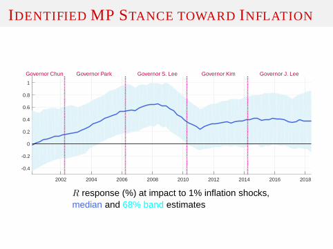
R response (%) at impact to 1% inflation shocks,median and 68% band estimates

Governor Chun Governor Park Governor S. Lee Governor Kim Governor J. Lee

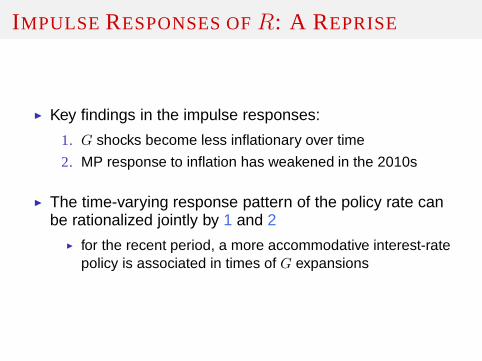
IMPULSE RESPONSES OF R: A REPRISE

◮ Key findings in the impulse responses:

1. G shocks become less inflationary over time

2. MP response to inflation has weakened in the 2010s

◮ The time-varying response pattern of the policy rate canbe rationalized jointly by 1 and 2

◮ for the recent period, a more accommodative interest-ratepolicy is associated in times of G expansions

Counterfactual Exercise

COUNTERFACTUAL IMPULSE RESPONSES

◮ Conduct a counterfactual experiment to net out how muchthe fall in the interest rate boosts the spending multiplier

◮ the counterfactual assumes that the interest rate did notchange in response to a G shock

◮ this can be implemented by using the actual VAR estimatedcoefficients from the other equations, while restricting thecoefficients in the interest rate rate equation to be zero

◮ e.g., Ramey (2013)

ACTUAL & COUNTERFACTUAL MULTIPLIERS

2005 2010 2015

0

0.05

0.1


2005 2010 2015

0

0.5

14 quarters

2005 2010 2015

0

0.5

1

1.5

8 quarters

2005 2010 2015

0

0.5

1

1.5

12 quarters

Actual Counterfactual

PV multiplier, actual and counterfactual estimates

DIFFERENCES IN THE PV MULTIPLIERS

2005 2010 2015-0.01

-0.005

0

0.005

0.01PV Multiplier Difference: Impact

2005 2010 2015

0

0.05

0.1

0.15

0.2

0.254 quarters

2005 2010 2015

-0.2

0

0.2

0.4

0.6

0.8

8 quarters

2005 2010 2015

-0.5

0

0.5

1

12 quarters

PV multiplier, actual minus counterfactual estimates

DIFFERENCES IN THE PV MULTIPLIERS

2000:Q2 2004:Q2 2008:Q2 2012:Q2 2016:Q2 2018:Q2

4 quarters 0.08 0.06 0.07 0.07 0.06 0.07[−0.02, 0.20] [0.00, 0.19] [−0.02, 0.21] [−0.01, 0.21] [−0.03, 0.21] [−0.03, 0.23]

8 quarters 0.13 0.18 0.28 0.33 0.30 0.24[−0.27, 0.48] [−0.10, 0.57] [−0.02, 0.75] [0.03, 0.80] [−0.03, 0.81] [−0.09, 0.82]

12 quarters 0.03 0.16 0.36 0.40 0.37 0.30[−0.59, 0.52] [−0.23, 0.69] [−0.06, 1.00] [0.00, 1.02] [−0.09, 1.05] [−0.17, 1.04]

Summary of the present-value multiplier gap estimates (in Korean won), median and [16%,84%] interval estimates

ACTUAL & COUNTERFACTUAL MULTIPLIERS

◮ Rossi and Zubairy (2011)◮ fiscal shocks are relatively more important in explaining

medium cycle fluctuations◮ MP shocks are relatively more important in accounting for

business cycle fluctuations

◮ Our finding: the effect of G shocks to output would havebeen much shorter-lived without the responses of R

Robustness Check

ROBUSTNESS 1: DROP OUT G

◮ The identified MP stance to inflation may be contaminatedby the incursion of gov’t spending as a model variable

◮ MP decisions are likely to be independent of FP actions

◮ Construct a 3-variable VAR specification without G

◮ obtain the responses of the policy rate to 1% inflationshocks

◮ compare them to their 4-variable baseline modelcounterpart

BASELINE VS. 3-VARIABLE VAR

2002 2004 2006 2008 2010 2012 2014 2016 2018

-0.4

-0.2

0

0.2

0.4

0.6

0.8

1

Baseline 3-variable VAR

R responses to π shocks, median and 68% band estimatesSolid: Benchmark; Dashed: 3-variable VAR without G

ROBUSTNESS 2: AUGMENT WITH TAXES

◮ Omission of another fiscal instrument, taxes (T ), may biasthe results

◮ the existing literature tends to include T as a model’sendogenous variable

◮ e.g., Blanchard and Perotti (2002); Ramey (2011)

◮ The responses of taxes to a gov’t spending shock can becrucial for the size of G multipliers

◮ if positive (negative), the expansionary effect of G shocks islikely to be mitigated (supplemented) by T responses

◮ Also, the sign of T responses at impact helps characterizethe financing source of the G expansion

◮ if positive (negative), the increase in G is initiallytax-financed (debt-financed)

ROBUSTNESS 2: AUGMENT WITH TAXES

◮ Expand the model by including taxes as an endogenousvariable

◮ The 5-variable VAR specification comprises {G, Y, π, T, R}

◮ The ordering is given as above

◮ T after Y and π can be rationalized that, given the tax rate,the tax base is contemporaneously affected by these twovariables, and thus tax receipts change

◮ Caldara and Kamps (2008)


2002 2006 2010 2014 2018

-1

-0.5

0

Tax Response: Impact

2002 2006 2010 2014 2018

-1

-0.5

0

0.5

1

4 quarters

2002 2006 2010 2014 2018

-0.5

0

0.5

1

8 quarters

2002 2006 2010 2014 2018

-0.5

0

0.5

1

12 quarters

T responses to G shocks, median and 68% band estimates


2002 2006 2010 2014 2018

0

0.05

0.1


2002 2006 2010 2014 2018

0

0.2

0.4

0.6

0.8

1

4 quarters

2002 2006 2010 2014 2018

0

0.5

1

1.5

8 quarters

2002 2006 2010 2014 2018

-0.5

0

0.5

1

1.5

12 quarters

PV multipliers, median and 68% band estimatesSolid: Benchmark; Dashed: 5-variable VAR augmented with T

Technical Appendix

APPENDIX 1: METHODOLOGY

◮ Assumptions: states follow random walks

Bt = vec([ct, B1,t, B2,t, B3,t)], Bt = Bt−1 + νt, νt ∼ NID(0, Q)

αt = vec(A−1

t ), αt = αt−1 + ζt, ζt ∼ NID(0, S)

σt = vec(diag(Σe,t)), log σt = log σt−1 + ηt, ηt ∼ NID(0,W )

◮ Informative but diffuse conditional prior distributions◮ calibrated based on 40 initial training samples (90:Q1-99:Q4)

◮ OLS estimates parameterize prior means, serve as startingvalues

◮ MCMC algorithm to generate sample from unknown jointposterior distribution p(BT ,ΣT

u , Q, S,W |ZT )

APPENDIX 2: SUMMARY OF GIBBS SAMPLER

1. Initialize AT , ΣTe , hyperparameters Q, S and W

2. Draw coefficients from p(BT |ZT , AT , Q), Carter-Kohn (1994)

3. Draw covariances from p(AT |ZT ,ΣTe , S), Carter-Kohn (1994)

4. Draw volatilities from p(ΣTe |Z

T , BT , AT ,W ), Carter-Kohn (1994)

5. Draw hyperparameters from p(Q|ZT , BT ), p(S|ZT , AT ),p(W |ZT ,ΣT

e )

6. Go to 2, generate 22k after 20k burn-in iterations

Measuring Time-varying Fiscal Multipliers

When Monetary Policy Matters∗

Jong-Suk Han† Joonyoung Hur‡

ABSTRACT

This paper empirically measures the change of the government spending multipliers since

2000 with a time-varying coefficient vector autoregressive(TVC-VAR) model. While estimat-

ing the multipliers, we explicitly take into account the monetary policy response measured by

interest rates. The present value fiscal multipliers in the long run have steadily increased after

the Global Financial Crisis. Moreover, our counterfactualexercise shows that the accommoda-

tive monetary policy stance enhances the long-run stimuluseffect of the government spending

on output.

Keywords: Time-varying coefficient VAR; Government spending multiplier; Monetary policy

JEL Classifications: C11; E32; E62; E52

∗We are grateful to Jinill Kim and Soyoung Kim for valuable discussions and comments. We also thank seminarparticipants at the Bank of Korea’s Research Department, Korea Institute for International Economic Policy and KoreaInstitute of Public Finance for helpful comments. The viewsexpressed in this paper are solely the responsibility ofthe authors and should not be interpreted as reflecting the views of the Korea Institute of Public Finance. This work issupported by Hankuk University of Foreign Studies ResearchFund of 2019.

†Center for Fiscal Projections, Korea Institute of Public Finance, 1924 Hannuri-daero, Sejong, Republic of Korea.Tel: +82-44-414-2415, E-mail:[email protected].

‡Corresponding author. Division of Economics, Hankuk University of Foreign Studies, 107, Imun-ro,Dongdaemun-gu, Seoul, Republic of Korea. Tel: +82-2-2173-8813, E-mail:[email protected].

HAN & H UR: MEASURING TIME-VARYING FISCAL MULTIPLIERS WHEN MP MATTERS

1 INTRODUCTION

The effects of expansionary government spending on macroeconomic aggregates depend on a host

of factors: expected sources of future fiscal financing [Uhlig (2010)], whether the implemented

policy is anticipated or not [Ramey(2011)], and how monetary policy behaves in times of the fiscal

expansion [Eggertsson(2008); Christiano et al.(2011); Erceg and Linde(2014)]. Among these, the

last dimension has received much recent attention, spurredprimarily by the fiscal stimuli associated

with the Federal Reserve’s zero interest rate policy in counteracting the global recession of 2008.

A burgeoning theoretical and empirical literature has developed in recent years, demonstrating that

fiscal effects are substantially larger at the lower bound for nominal interest rates.

Taken in a more general sense, the zero lower bound is regarded as a special case in which

central banks’ concerns shift away from their central objective—inflation targeting—toward other

goals, such as output or financial stabilization [e.g.,Board of Governors of the Federal Reserve

System(2009) andBank of England(2009)]. One of the main characteristics of the policy behavior

is that the monetary authority does not increase nominal rates strongly with inflation. A stream of

literature, includingKim (2003), Davig and Leeper(2011), andDupor and Li(2015), documents

that expansionary effects of government spending are much more pronounced when this type of

policy environment is in place.

This paper attempts to assess empirically how fluctuations in monetary policy behavior affect

the stimulus effects of government spending expansions. Weparticularly take into account Korea

as a laboratory for this avenue due to the following reasons.First, a structural break in the Korean

macroeconomic aggregates is observed, which may incur potential changes in the monetary policy

behavior. Figure1 shows the series for output, inflation, and the policy interest rate for the period

2000:Q1−2018:Q2. Focusing on output and inflation, the volatilitiesof these variables decline

substantially in the 2010s, compared to their 2010s counterpart. What is more striking, though,

is the disparity in the level of inflation across the two decades. Inflation started falling with the

beginning of the 2010s so that its overall level for the subsequent period is dramatically lower

than that of the 2000s. The policy rate over the sample periodtends to fluctuate with the level

of inflation. Given the sharp contrast in the levels of inflation, however, the responsiveness of

monetary policy toward inflation deserves careful scrutiny.

Second, the behavior of monetary policy in times of fiscal expansions turns out to be quite ac-

commodative over the sample. To inspect this in a formal manner, we estimate a 4-variable vector

autoregressive (VAR) model comprising of government spending, output, inflation and the nomi-

nal policy rate. The impulse responses to an identified government spending shock are provided

1


in Figure2.1 The results show that an increase in government spending stimulates output in the

medium to longer runs. Its impacts on inflation are negative for the short horizons, though they are

not significantly different from zero at conventional levels. A more notable finding emerges from

the interest rate response. An increase in government spending leads to a significant fall in the

policy rate, suggesting that the periods of fiscal expansions throughout the sample are on average

associated with monetary accommodation.

Based on these features, the contribution of this paper is toidentify a time-varying pattern in

government spending multipliers of Korea and to net out the contribution of monetary policy in

shaping the stimulus effects. We employ a time-varying coefficient VAR (hereafter TVC-VAR)

model as inPrimiceri (2005) andGalı and Gambetti(2015). The model is estimated with Korean

data ranged from 2000:Q1 to 2018:Q2. The selection of the sample period is constrained by the

shift in monetary policy occurring in the late 1990s.Brito and Bystedt(2010) andChoi and Hur

(2015) document that the post-2000s period corresponds to an inflation targeting regime, whereas

this evidence is hardly supported by data in the precedent period.

The results show that monetary policy responses to inflationvary considerably within the sam-

ple. The central bank’s stance toward inflation turns out to be quite mild during the early years of

the sample, whereas the second half of the 2000s is marked with a stronger reaction to inflation

over time up to the onset of the global financial crisis (GFC) of 2008-09. For the remainder of the

sample, the degree of policy responsiveness bounces back only marginally but not fully compared

to its peak in the late 2000s.

A number of notable time-varying patterns in macroeconomicaggregates followed by gov-

ernment spending expansions are observed from the results.First, government spending shocks

become less inflationary over time. In particular, the inflation responses become negative for the

post-GFC period in terms of the median estimates. Second, the nominal interest rate falls in re-

sponse to government spending expansions, and the plunges in the interest rate associated with

government spending shocks are more pronounced in the recent sample. Together with the afore-

mentioned monetary policy response toward inflation, the first finding may provide an important

insight in understanding the accommodative behavior of theinterest rate in times of government

spending increases. Taken together the findings that monetary policy response to inflation has

weakened in the 2010s and that government spending shocks become less inflationary as time

elapses, a more accommodative interest-rate policy in the recent period can be associated with

increases in government spending.

We demonstrate that the accommodative monetary policy in times of government spending

1The empirical procedure used for the results of Figure2 is detailed in Section2.

2


expansions is a critical determinant of the size of government spending multipliers. More specifi-

cally, the expansionary effect of government spending on output is a lot more pronounced for the

recent period than in the 2000s. For instance, the peak multiplier for 20004:Q2 is 0.51, whereas the

2016:Q2 multiplier turns out to be 0.88, which is more than 50% higher in size. We also find that

monetary policy stance matters a lot for the longer-run stimulus effects of government spending

than the short-runs.

2 ECONOMETRICSPECIFICATION

This article utilizes a TVC-VAR model to characterize how the expansionary effects of government

spending change over time. In this section, we illustrates the VAR model specification employed

in this paper.

2.1 VAR WITH TIME-VARYING COEFFICIENTS The reduced-form VAR specification is given

as

zt = µ0,t + µ1t + µ2t2 +Dxt +B1,tzt−1 + . . .+Bℓ,tzt−ℓ + ut, t = 1, . . . , T, (1)

whereµ0,t is ann×1 vector of time-varying constant terms, andt andt2 denote linear and quadratic

time trends, respectively.xt is anm × 1 vector of observed exogenous variables with the time-

invariant coefficient matrixD. zt is ann × 1 vector of observed endogenous variables andBi,t

with i = 1, . . . , ℓ aren × n matrices of time-varying coefficients associated with the endoge-

nous variables.ut are heteroskedastic reduced-form errors withE(utu′

t) = Σu,t. Notice that the

reduced-form disturbances are be correlated with each other, i.e., the off-diagonal elements ofΣu,t

are non-zero.

The choice of the exogenous variables is to reflect the Koreaneconomy’s feature as a small

open economy. FollowingKim (2000), we consider the US federal funds rate, the growth rate of

oil prices, and the real exchange rate of Korean won against the US dollar in order to control for

the potential factors affecting the central bank’s policy decision. In addition, US output is included

as a proxy for the world business cycle.2

In order to assess the effects of government spending on output conditioning on the monetary

policy, we have the minimal set of endogenous variables as{gt, yt, πt, rt}, wheregt is government

spending,yt is output,πt is inflation rate, andrt is the nominal interest rate.gt andyt are essential

in measuring the expansionary effects of government spending, often referred to as government

spending multipliers.3 The inclusion of inflation and the nominal interest rate is tocomplete the

2AppendixA provides a detailed description of the data used in this paper.3Using these two variables,Caldara and Kamps(2017) demonstrate that the size of government spending multipli-

ers hinges critically upon the identification strategies ofgovernment spending shocks.

3


monetary policy block associated with the central bank’s dual mandate—output and price stability.

The set of variables{yt, πt, rt} is often regarded as the minimal sufficient statistic in summarizing

the central banks’ dual mandate behavior [e.g.,Primiceri(2005) andCoibion(2012), among many

others]. Based on the information criteria such as AIC and BIC, the lag of the VAR specification

is set to beℓ = 3.

The corresponding structural VAR is written as

Atzt = At

(

µ0,t + µ1t + µ2t2 +Dxt

)

+ AtB1,tzt−1 + AtB2,tzt−2 + AtB3,tzt−3 + et, (2)

At eacht, consider the lower-triangular Cholesky decomposition ofthe covariance matrixΣu,t

which yields

Atut = et, (3)

whereet are the structural innovations with the covariance matrixE(ete′

t) = Σe,t so thatAtΣu,tA′

t =

Σe,tΣ′

e,t with

At =

1 0 0 0

α21,t 1 0 0

α31,t α32,t 1 0

α41,t α42,t α43,t 1

, Σe,t =

σ2

e1,t 0 0 0

0 σ2

e2,t 0 0

0 0 σ2

e3,t 0

0 0 0 σ2

e4,t

.

In this article, we order the endogenous variables as follows: government spending is ordered

first, output is ordered second, inflation is ordered third, and the nominal interest rate is ordered

last. This particular ordering has the following implications: (i) government spending is the most

exogenous, and thus has no contemporaneous responses to shocks to other variables in the system

[e.g.,Fatas and Mihov(2001) andBlanchard and Perotti(2002)]; (ii) output does not react to infla-

tion and interest rate shocks in the same period, but is affected contemporaneously by government

spending shocks; (iii) inflation does not react contemporaneously to interest rate shocks, but is

affected contemporaneously by government spending and output shocks; and (iv) the interest rate

is affected contemporaneously by all shocks in the system. Placing output and inflation in front of

the nominal interest rate can be justified on the grounds thatinterest rate-based monetary policy

decisions are conditioning on output and inflation of the concurrent period.

4


2.2 STATE-SPACE REPRESENTATION OF THEVAR SPECIFICATION The reduced-form VAR

in (1) has a state-space representation as follows:

[Observation equation] zt = Z ′

tBt + ut, Z ′

t = In ⊗ [1, z′t−1, . . . , z′t−ℓ], (4)

[State equation] Bt = Bt−1 + νt, (5)

where the symbol⊗ denotes the Kronecker product. FollowingPrimiceri (2005) andGalı and

Gambetti(2015), we make two assumptions on the time-varying parameters inthe model: (i) the

elements of the matricesAt andΣu,t follow an AR(1) process; and (ii) all the innovations in the

model are multivariate normal. Thus, the dynamics of the model’s time-varying parameter can be

summarized as follows:

αt =αt−1 + ζt, log σt = log σt−1 + ηt,

V =V ar

ut

νt

ζt

ηt

=

In 0 0 0

0 Q 0 0

0 0 S 0

0 0 0 W

,

whereαt denotes the column vector of the lower-triangular elementsof the matrixAt stacked by

rows,σt is the column vector of the diagonal elements of the matrixΣe,t, andQ, S, andW are

positive definite matrices. In sum, we have following time-varying parameters to be estimated:

[Coefficients of the reduced-form VAR] BT := {B1, . . . , BT} ,

[Elements of the Cholesky factor] AT := {A1, . . . , AT} ,

[Variances of the structural VAR] ΣTe := {Σe,1, . . . ,Σe,T} ,

[Variance-covariance matrices of the innovations]V.

2.3 DATA AND ESTIMATION The aforementioned TVC-VAR model is estimated using quar-

terly data from 1990:Q1 to 2018:Q2. The first 10-year sample,ranged between 1990:Q1 and

1999:Q4, is used to initiate the prior distributions for theTVC-VAR model so that the actual sam-

ple period for empirical analyses is from 2000:Q1 to 2018:Q2. The choice of the sample period for

empirical analyses is due primarily to the shift in monetarypolicy occurring in the late 1990s.Brito

and Bystedt(2010) andChoi and Hur(2015) document that the post-2000s period corresponds to

an inflation targeting regime, whereas this evidence is hardly supported by data in the precedent

period.

5


The estimation procedure of the TVC-VAR model follows that of Primiceri (2005) andGalı

and Gambetti(2015). We employ independent inverse-Wishart prior distributions for the hyperpa-

rametersQ, W , andS. The priors for the initial values forB0, α0, andlog σ0 are assumed to be

normally distributed. As a result, the entire sequences ofB, α, andlog σ are normally distributed

conditioned onQ, W , andS. The posterior distributions of the model’s parameters areobtained

by using Gibbs sampling, which simulates 22,000 posterior draws, with the first 20,000 used as a

burn-in period and every 2nd thinned, leaving a sample size of 1,000.4

3 EMPIRICAL RESULTS

This section documents the posterior estimates for the impulse responses from the aforementioned

TVC-VAR model. To begin, we report the identified central bank’s stance toward inflation, which

will be critical in shaping the expansionary effects of government spending shocks. We then pro-

vide the time-varying pattern in government spending multipliers and unveil their crucial determi-

nant by conducting a counterfactual experiment.

3.1 IDENTIFIED MONETARY POLICY STANCE TOWARD INFLATION Figure3 reports the time-

varying impulse responses of the nominal interest rateat impactassociated with 1% increases in

inflation. To connect this result with narrative accounts ofmonetary policy history in Korea, we

additionally provide the vertical lines indicating the Bank of Korea governor terms. As inPrimiceri

(2005), notice that the object in this figure can be interpreted as the contemporaneousmonetary

policy stance toward inflation, and thus corresponds to the Taylor rule inflation coefficient of fully

structural general equilibrium models.

Monetary policy responses to inflation turn out to be quite mild during the early years of the

sample. In order to achieve price stability via an Inflation Targeting system, the Bank of Korea

made its policy shift from the money aggregate based approach to the interest rate based policy in

1998. Hence, the weak response during the first half of the 2000s may stem from the monetary

policy turning point just prior to the sample period.

The second half of the 2000s is marked with a stronger reaction to inflation over time up to

the onset of the global financial crisis (GFC) of 2008-09. Consequently, monetary policy was the

most hawkish under the Seongtae Lee’s governorship. This upward tendency, however, did not

last long. Shortly after, confronting a severe economic downturn associated with the GFC, there

were two consecutive cuts of the policy rate in the first quarter of 2009. The interest rate fell from

4.05 (2008:Q4) to 1.88 (2009:Q2) percent per annum, an unprecedented low level in the Korean

4Please refer toGalı and Gambetti(2014) for a detailed description of the sampling algorithm used in this article.

6


monetary policy history. Our TVC-VAR estimates suggest that the central bank’s response toward

inflation declines with these policy actions.

For the remainder of the sample, the degree of policy responsiveness bounces back only marginally

but not fully compared to its peak in the late 2000s. Our estimates indicate that the central bank’s

stance toward inflation is not much different from its mid-2000s level. Notice, however, that the

level of inflation over this period is somewhat lower than that of the 2000s, as depicted in Figure1.

Taken together, the TVC-VAR result shows that the mild reaction to inflation in the recent period

can be justified in light of the low inflation environment.

3.2 EFFECTS OFGOVERNMENT SPENDING SHOCKS We now inspect the macroeconomic con-

sequences of government spending shocks, associated with the TVC-VAR model. In the existing

literature, the expansionary effects of government spending on output are often summarized by a

present value multiplier defined as follows:

Present Value Multiplier(Q) =

∑Q

t=0(1 + r)tyt

∑Q

t=0(1 + r)tgt

1

Y /G(6)

where r andG/Y denote the sample means of the real interest rate and share ofgovernment

spending in GDP, respectively.

Figure4 shows the median estimates of present value multipliers. The figure makes clear that

the effects of increases in government spending on output vary substantially over time, pronounced

more in the longer horizons. In particular, the longer-run multipliers tend to spike up in the 2010s.

As a result, the shape of present value multipliers changes as time elapses—from a hump-shaped

response pattern in the early 2000s to a monotonically increasing one after the GFC period. Since

present value multipliers represent the full dynamics of discounted future macroeconomic effects

caused by exogenous changes in government spending, this finding indicates that an increase in

government spending has more persistent effects on output in the recent sample.

To conduct full statistical analyses of the results, Figures5 through7 plot the median and 68%

band estimates of present value multipliers as well as of theimpulse responses of inflation and the

nominal interest rate for selected horizons—at impact, and4, 8 and 12 quarters after government

spending shocks. First of all, the sliced present value multipliers are reported in Figure5. Although

neither substantial in size nor statistically different from zero, it turns out that the impact multipliers

keep increasing over time. The pattern, however, is quite different for the 4-quarter multipliers as

in the second panel of the figure. Present value multipliers show a decreasing tendency from the

beginning of the sample to the GFC period, but they bounce back afterward. Accordingly, the

early 2000s and most of the 2010s correspond to the periods inwhich the expansionary effects of

7


government spending become significant in terms of the one-year estimates. For longer horizons,

present value multipliers display a similar pattern as theyhave no trend and remain statistically

indifferent from zero throughout the 2000s, and then rise tobecome significant in the 2010s.

In order to illustrate the differences in dynamics over time, Table1 reports the median estimates

of the present value multipliers for selected periods and horizons. Two findings stand out from

the peak multipliers. First, based on the peak multipliers,the expansionary effect of government

spending on output is a lot more pronounced for the recent period than in the 2000s. For instance,

the peak multiplier for 20004:Q2 is 0.51, whereas the 2016:Q2 multiplier turns out to be 0.88,

which is more than 50% higher in size. Second, the persistence effects of government spending

on output change over time. In the early 2000s, the peak multipliers appear at relatively shorter

horizons. This tendency, however, change dramatically forthe remainder of the sample so that

it takes more than 30 quarters for the maximum effect of government spending on output to be

realized. This finding suggests that government spending shocks tend to have more persistent

effects on output in the recent sample.

Figure6 provides the median and 68% band estimates of inflation impulse responses to gov-

ernment spending shocks for selected horizons. We do not observe any inflationary pressure due to

the fiscal expansions for all horizons considered, as the 68%band estimates always include zero.

This response pattern of inflation is somewhat puzzling based on a conventional macroeconomic

theory such as an IS-LM-type environment. Notice, however,that negative inflation responses to

a rise in government spending are often documented by the existing VAR studies with US data

includingFatas and Mihov(2001), Caldara and Kamps(2008) andMountford and Uhlig(2009).

Nevertheless, the response pattern at impact deserves further attention. The inflation responses

display a decreasing tendency as time elapses, and they become negative for the post-GFC period

in terms of the median estimates. Together with the monetarypolicy response toward inflation

described in Figure3, this finding may provide an important insight into how monetary policy in

times of government spending expansions is conducted.

In order to examine this issue in detail, Figure7 plots the impulse responses of the nominal

interest rate to government spending shocks. For the impactperiod, the responses are negative and

statistically different from zero over the whole sample period, consistent with the fixed-coefficient

VAR result in Figure2. When compared to the previous period, it is notable that themagnitude of

the negative response becomes more pronounced in the 2010s.The downward trend in the inflation

responses is also observed for the 4- and 8-quarter estimates. This response pattern can be ratio-

nalized by taking together the findings that monetary policyresponse to inflation has weakened

in the 2010s (Figure3) and government spending shocks become less inflationary astime elapses

8


(Figure6). Hence, a more accommodative interest-rate policy can be associated with increases in

government spending. An important implication of the rationale is that the expansionary effects of

government spending increases are amplified by the accommodative monetary policy, particularly

standing out in the 2010s. The subsequent section takes thisissue into consideration by conducting

a counterfactual exercise with a hypothetical monetary policy behavior during government spend-

ing expansions.

3.3 COUNTERFACTUAL IMPULSE RESPONSES To assess how much the fall in the interest rate

intensifies the present value multiplier, we pursue a counterfactual experiment in which the policy

rate did not change in response to government spending shocks. This empirical strategy is proposed

by Ramey(2013) in controlling for tax changes caused by an exogenous increase in government

spending. In a similar vein, we apply the methodology in order to mute the interest rate response

followed by government spending shocks. As provided inRamey(2013), the counterfactual exer-

cise can be implemented by using the actual VAR estimated coefficients from the other equations,

while restricting the coefficients in the interest rate rateequation to be zero.

Figure8 makes a comparison between the actual and counterfactual present value multipliers

for selected horizons. The gap across the two types of estimates is substantial, highlighted more

as the horizon increases. When associated with the counterfactual scenario, the 4-quarter present

value multiplier estimates show a similar time-varying pattern to their actual ones, with a slight

decrease in level. This tendency, however, does not hold forthe 8- and 12-quarter estimates.

The counterfactual multipliers associated with these horizons keep displaying a V-shaped pattern,

which is quite different from their actual counterparts.

In order to focus on the differences in dynamics across the two scenarios, Figure9 reports the

median and 68% error bands for the gap between the actual and counterfactual multiplier estimates.

As in the first panel of the figure, the gap across the two multipliers is minuscule at impact but

increases with horizons. As a result, the counterfactual scenario makes significant differences in

the first half of the 2010s based on the 8- and 12-horizon estimates. The only difference across

the two scenarios is the interest rate response to government spending shocks, so the disparity

in results corresponds to the role created by monetary policy behavior in times of government

spending expansions. Thus this finding suggests that the recent surge in government spending

multipliers reported in Figure5 is in part shaped by the accommodative stance of monetary policy.

Finally, Table2 tabulates the median and 68% estimates of the gap between theactual and coun-

terfactual present value multipliers for selected periodsand horizons. Focusing on the 2012:Q3

estimates when the gap is most pronounced and significant, 33% and 40% additional expansionary

effects of government spending on output are attributable to the particular monetary policy behav-

9


ior in terms of the median values. Although not significant, this effect seems to prevail throughout

the 2010s. These findings have implications that extend beyond the exercises performed here—in

principle, the monetary policy stance can have major implications for fiscal impacts.

4 ROBUSTNESSCHECK

4.1 IDENTIFIED MONETARY POLICY STANCE In gauging the monetary policy stance toward

its stabilizing objectives, a potential concern associated with the framework in this article is whether

the results are contaminated by the inclusion of governmentspending as a model’s endogenous

variable. This is because conventional monetary policy analyses tend to be embedded only with

variables relevant to monetary policy decisions, and government spending is unlikely to be one of

them. In this regard, a robustness check may be necessary to inspect if our result in Figure3 is con-

fronted with this issue. Accordingly, we construct a 3-variable VAR system without government

spending so that the model contains the policy rate as well asthe dual mandate objectives—output

and inflation.

Figure10plots the impulse responses of the nominal interest rate to 1% inflation shocks (dotted

lines), together with their baseline 4-variable model counterpart (solid line with shaded area). The

impulse responses from the 3-variable model display slightly tighter band estimates than those

from the 4-variable VARs. This tendency may be attributableto the “curse of dimensionality”

problem, typically associated with TVC-VARs of many additional parameters to be estimated as

the number of variables increase. Nevertheless, it is worthnoting that the overall pattern of the

responses remains quite similar to that of the baseline specification. The response pattern in the

2000s remains almost identical when government spending isexcluded. For the subsequent pe-

riod, the responses across the two models are quantitatively different, but not qualitatively. The

responses with the 3-variable system are constantly higherthan those of the baseline specification.

However, the fact that monetary policy becomes less hawkishin the 2010s than its peak response

in the late 2000s is almost unaltered under the 3-variable model.

4.2 CONTROLLING FOR TAXES As demonstrated inRossi and Zubairy(2011) and Ramey

(2013), how taxes behave in response to a government spending shock may have a crucial im-

plication for the size of government spending multipliers.Guided by the findings in the existing

literature, our second robustness check is to augment the model with taxes.

To this end, we specify a 5-variable VAR system consisting ofgovernment spending, output,

inflation, taxes and the nominal interest rate. Notice that this set of variables is the ones em-

ployed inPerotti(2005) andCaldara and Kamps(2008). Following Caldara and Kamps(2008),

the identification of government spending shocks relies on the recursive ordering as listed above.

10


Ordering taxes after output and inflation can be rationalized that, given the tax rate, the tax base is

contemporaneously affected by these two variables, and thus tax receipts change.

Focusing first on the impulse responses of taxes, two findingsemerge from Figure11. First,

there is no clear time-varying pattern in the tax responses.Second, the impulse responses of taxes

are statistically indifferent from zero for all the periodsand horizons considered, with an exception

of the impact responses in the early 2000s. It is, however, noticeable that the tax responses at

impact provide a characterization of government spending shocks over the sample period. Taxes

decrease at impact in response to increases in government spending, indicating that the identified

government spending shocks are initially deficit financed.

Figure12plots the present value multiplier estimates for selected horizons, associated with the

5-variable (dotted lines) and baseline 4-variable (solid line with shaded area) VAR specifications.

Despite the decreases in taxes at impact, the present value multipliers up to 4 quarters remain

almost unaltered by augmenting the model with taxes. The longer run multipliers tend to become

slightly smaller under the 5-variable system, but the differences are only marginal as its 68% bands

mostly overlap with those of the 4-variable benchmark. Hence, we find that controlling for taxes

does not alter substantially the quantitative estimates ofgovernment spending multipliers.

5 CONCLUSION

After the Global Financial Crisis, the growth rate in Korea has steadily declined despite the low

output volatility. In order to boost up the economic growth,the expansionary fiscal policy has been

conducted since 2010. At the same time, the monetary policy has been less hawkish during these

active fiscal policy regimes. Under this situation, our paper empirically assesses the effects of ex-

pansionary government spending on output changes over time, and investigate the role of monetary

policy stance on the multipliers. We tackle these problems with a time-varying coefficient VAR

model recently developed.

We apply TVC-VAR model in Korea from 2000:Q1 to 2018:Q2 with 4endogenous variables,

government spending, output, inflation and nominal interest rates. In order to reflect the small open

economy features in Korea, we exogenously control some variables such as US federal funds rate,

oil prices changes, the real exchange rate of Korean Won against the US dollar, and US output

as a proxy for the world business cycle. The present value spending multipliers display some

interesting trend across different time horizons. The impact multipliers have steadily increased

overtime but the 4-quarter multipliers display V-shaped with the turning points at 2008. The 8-

quarter and 12-quarter multipliers, however, significantly increased after GFC. On the other hand,

the monetary policy stance, measured with the response of nominal interest rate to 1% increases of

11


inflation, were more active until the GFC but moved toward relative passive stance after 2010. In

order to examine the effects of the monetary policy changes on the fiscal multipliers, we perform a

counterfactual analysis by restricting the coefficients inthe interest rate equation to be zero. When

monetary policy does not react to the economic shocks, the fiscal multipliers are significantly

dropped compared to the baseline results. Specially, the differences are pronounced in the 8-

quarter and 12-quarter multipliers after the GFC.

Our results have some important implications. For Korean economy point of view, we find

that the recent expansionary fiscal policy has positive impact on the output growth especially in

the long run. The 8-quarter and 12-quarter fiscal multipliers are significantly improved after the

GFC. Next, these improvement in the long-run multipliers are supported by the accommodative

monetary policy. As discussed before, the monetary policy stance has an important consequence

to an expansionary fiscal policy. This viewpoint is supported by various empirical results from

US. Our results from Korea is in line with these researches, and supports that the accommodative

monetary policy stance can amplify the fiscal multipliers and the amplification is stronger in the

long-run.

12


A DATA

We employ Korean data from 1990:Q1 to 2018:Q2 for the endogenous variables of the VAR mod-els. Our VAR specifications also include four exogenous variables which use quarterly data for thegrowth rate of oil price, federal funds rate, US real GDP per capita, and real exchange rate againstdollar. Detailed data descriptions are as follows:

Government Spending =log(Domestic Real Per Capita Government Spending),

GDP = log(Domestic Real Per Capita GDP),

Inflation Rate =log(Domestic CPI/Domestic CPI(−1)) × 100,

Taxes =log(Domestic Real Per Capita Taxes),

Nominal Interest Rate = Domestic Overnight Call Rate,

Growth Rate of Oil Pirce =log(Oil Price/Oil Price(−1))× 100,

US Nominal Interest Rate = US Federal Funds Rate,

US GDP = log(US Real Per Capita GDP),

Real Exchange Rate = Nominal Exchange Rate (won/dollar)× US CPI/Domestic CPI.

For the construction of the real per capita variables, domestic and US real series are divided by the

corresponding country’s population, except for the Koreanfiscal data. Only seasonally unadjusted

nominal variables are available for the Korean fiscal variables—government spending and taxes.

They are therefore deseasonalized by using the X-13-ARIMA procedure and converted into real

variables based on the domestic CPI. US GDP uses the real series. The original data and their

sources are given as follows:

• Domestic Nominal Government Spending: Total government spending expenditure, not sea-

sonally adjusted / Source: Korean Statistical InformationService (KOSIS)

• Domestic Real GDP: Real gross domestic product, seasonallyadjusted / Source: The Bank

of Korea’s Economic Statistics System Database (BOK-ECOS)

• Domestic CPI: Consumer price indexes, 2015=100, seasonally adjusted / Source: BOK-

ECOS

• Domestic Nominal Taxes: Total tax revenue, not seasonally adjusted / Source: KOSIS

• Domestic Nominal Interest Rate: Overnight call rate, uncollateralized, percent per annum,

averages of daily figures / Source: BOK-ECOS

• Domestic Population: Total population, annual / Source: KOSIS

13


• Oil price: Global price of Dubai Crude, US dollars per barrell, quarterly, not seasonally ad-

justed / Source: Federal Reserve Economic Data (FRED, St. Louis Fed), Series ID “POIL-

DUBUSDM”

• US Federal Funds Rate: Averages of daily figures, percent / Source: Board of Governors of

the Federal Reserve System

• US Real GDP: Real gross domestic product, chained dollars, billions of chained (2009)

dollars, seasonally adjusted at annual rates / Source: NIPATable 1.1.6, Line 1

• Nominal Exchange Rate: Won/dollar exchange rate / Source: BOK-ECOS

• US CPI: Consumer price index for all urban consumers, all items, index 1982−1984=100,

quarterly, seasonally adjusted / Source: FRED, Series ID “CPIAUCSL”

• US Population: Civilian noninstitutional population, ages 16 years and over, seasonally ad-

justed / Source: US Department of Labor, Bureau of Labor Statistics

14


B TABLES

2000:Q2 2004:Q2 2008:Q2 2012:Q2 2016:Q2 2018:Q2

Impact 0.02 0.03 0.04 0.05 0.05 0.05

4 quarters 0.43 0.33 0.39 0.39 0.43 0.42

8 quarters 0.52 0.49 0.29 0.70 0.75 0.67

12 quarters 0.44 0.50 0.15 0.78 0.82 0.75

Peak (QTR) 0.54 (7) 0.51 (11) 0.65 (39) 0.85 (39) 0.88 (30) 0.82 (31)

Table 1: Median estimates of the present value multipliers for selected periods and horizons. The numbers reported inthis table represent GDP responses in Korean won to initial increases in government spending by one Korean won.

2000:Q2 2004:Q2 2008:Q2 2012:Q2 2016:Q2 2018:Q2

4 quarters 0.08 0.06 0.07 0.07 0.06 0.07

[−0.02, 0.20] [0.00, 0.19] [−0.02, 0.21] [−0.01, 0.21] [−0.03, 0.21] [−0.03, 0.23]

8 quarters 0.13 0.18 0.28 0.33 0.30 0.24

[−0.27, 0.48] [−0.10, 0.57] [−0.02, 0.75] [0.03, 0.80] [−0.03, 0.81] [−0.09, 0.82]

12 quarters 0.03 0.16 0.36 0.40 0.37 0.30

[−0.59, 0.52] [−0.23, 0.69] [−0.06, 1.00] [0.00, 1.02] [−0.09, 1.05] [−0.17, 1.04]

Table 2: Gap between the actual and counterfactual present value multipliers for selected periods and horizons. Medianand [16%, 84%] estimates are reported.

15


C FIGURES

2002 2004 2006 2008 2010 2012 2014 2016 2018-4

-2

0

2

Output

Quad. detrendedHP filtered

2002 2004 2006 2008 2010 2012 2014 2016 2018

0

0.5

1

1.5

2

Inflation Rate and Nominal Interest Rate

InflationOvernight call rate

Figure 1: Time series for the macroeconomic aggregates in Korea, from 2000:Q1 to 2018:Q2.[Left panel] Real percapita output, quadratic detrended (solid line) and HP-filtered (dashed line).[Right panel] Quarterly inflation rate(solid line) and nominal interest rate (overnight call rate, dotted line).

0 5 10 15 20

0

0.5

1

Government Spending

0 5 10 15 20

-0.02

0

0.02

Output

0 5 10 15 20

-0.02

-0.01

0

0.01

Inflation Rate

0 5 10 15 20

-0.06

-0.04

-0.02

0

Nominal Interest Rate

Figure 2: Impulse responses to a 1% increase in government spending, associated with the fixed coefficient VARmodel. In each panel, point estimate (solid line) and 68% confidence interval estimates (dashed lines) are reported.The x-axis measures quarters.

16


2002 2006 2010 2014 2018

0

0.5

1Governor Chun Governor Park Governor S. Lee Governor Kim Governor J. Lee

Figure 3: Time-varying impulse responses of the interest rate at impact to 1% increases in inflation, associated with theTVC-VAR model. Median (solid line) and 68% band (shaded area) estimates are reported. The vertical lines indicatethe Bank of Korea governor terms.

40

0.2

0.4

30 20182016

0.6

201420

0.8

20122010200810 2006200420020

Figure 4: Time-varying present value multipliers, associated with the TVC-VAR model. Median estimates are re-ported.

17


2002 2006 2010 2014 2018

0

0.05

0.1


2002 2006 2010 2014 2018

0

0.5

14 quarters

2002 2006 2010 2014 2018

0

0.5

1

1.5

8 quarters

2002 2006 2010 2014 2018

0

0.5

1

1.5

12 quarters

Figure 5: Time-varying present value multipliers for selected horizons, associated with the TVC-VAR model. In eachpanel, median (solid line) and 68% band (shaded area) estimates are reported.

2002 2006 2010 2014 2018

-0.1

-0.05

0

0.05

Inflation Response: Impact

2002 2006 2010 2014 2018-0.04

-0.02

0

0.02

0.04

0.06

4 quarters

2002 2006 2010 2014 2018

-0.02

0

0.02

8 quarters

2002 2006 2010 2014 2018

-0.01

0

0.01

0.0212 quarters

Figure 6: Time-varying impulse responses of inflation to 1% increases in government spending for selected horizons,associated with the TVC-VAR model. In each panel, median (solid line) and 68% band (shaded area) estimates arereported.

18


2002 2006 2010 2014 2018-0.3

-0.2

-0.1

0Interest Rate Response: Impact

2002 2006 2010 2014 2018

-0.2

0

0.2

4 quarters

2002 2006 2010 2014 2018

-0.1

0

0.1

8 quarters

2002 2006 2010 2014 2018

-0.1

-0.05

0

0.05

12 quarters

Figure 7: Time-varying impulse responses of the interest rate to 1% increases in government spending for selectedhorizons, associated with the TVC-VAR model. In each panel,median (solid line) and 68% band (shaded area)estimates are reported.

2002 2006 2010 2014 2018

0

0.05

0.1


2002 2006 2010 2014 2018

0

0.5

14 quarters

2002 2006 2010 2014 2018

0

0.5

1

1.58 quarters

2002 2006 2010 2014 2018

0

0.5

1

1.5

12 quarters

Actual Counterfactual

Figure 8: Actual (solid line with shaded area) and counterfactual (dashed lines) time-varying present value multipliersfor selected horizons, associated with the TVC-VAR model. In each panel, median and 68% band estimates arereported. The counterfactual impulse responses are calculated under the assumption that the nominal interest rate didnot change in response to government spending shocks.

19


2002 2006 2010 2014 2018-0.01

0

0.01PV Multiplier Difference: Impact

2002 2006 2010 2014 2018

0

0.1

0.2

4 quarters

2002 2006 2010 2014 2018

-0.2

0

0.2

0.4

0.6

0.8

8 quarters

2002 2006 2010 2014 2018

-0.5

0

0.5

1

12 quarters

Figure 9: The differences between actual and counterfactual time-varying present value multipliers for selected hori-zons, associated with the TVC-VAR model. In each panel, median (thick dash-dot line) and 68% band (thin dash-dotlines) estimates are reported. The counterfactual impulseresponses are calculated under the assumption that the nom-inal interest rate did not change in response to government spending shocks.

2002 2006 2010 2014 2018

0

0.5

1

Baseline 3-variable VAR

Figure 10: Time-varying impulse responses of the interest rate at impact to 1% increases in inflation, associated withthe benchmark TVC-VAR model with 4 variables (solid line with shaded area) and the 3-variable TVC-VAR modelwithout government spending (dotted lines), respectively. Median and 68% band estimates are reported. The verticallines indicate the Bank of Korea governor terms.

20


2002 2006 2010 2014 2018

-1

-0.5

0

Tax Response: Impact

2002 2006 2010 2014 2018-1

-0.5

0

0.5

1

4 quarters

2002 2006 2010 2014 2018

-0.5

0

0.5

1

8 quarters

2002 2006 2010 2014 2018

-0.5

0

0.5

112 quarters

Figure 11: Time-varying impulse responses of taxes to 1% increases in government spending for selected horizons,associated with the 5-variable TVC-VAR model augmented with taxes. In each panel, median (thick dotted line) and68% band (thin dotted lines) estimates are reported.

2002 2006 2010 2014 2018

0

0.05

0.1


2002 2006 2010 2014 2018

0

0.5

1

4 quarters

2002 2006 2010 2014 2018

0

0.5

1

1.5

8 quarters

2002 2006 2010 2014 2018

-0.5

0

0.5

1

1.5

12 quarters

Figure 12: Time-varying present value multipliers for selected horizons, associated with the benchmark TVC-VARmodel with 4 variables (solid line with shaded area) and the 5-variable TVC-VAR model augmented with taxes (dottedlines). In each panel, median and 68% band estimates are reported.

21


REFERENCES

BANK OF ENGLAND (2009): “Minutes of the Monetary Policy Committee Meeting,” London,

March 4 and 5.

BLANCHARD , O. AND R. PEROTTI (2002): “An Empirical Characterization of the Dynamic Ef-

fects of Changes in Government Spending and Taxes on Output,” Quarterly Journal of Eco-

nomics, 117, 1329–1368.

BOARD OF GOVERNORS OF THEFEDERAL RESERVESYSTEM (2009): “Monetary Policy Report

to Congress,” Washington, D.C., July 21.

BRITO, R. D. AND B. BYSTEDT (2010): “Inflation Targeting in Emerging Economies: Panel

Evidence,”Journal of Development Economics, 91, 198–210.

CALDARA , D. AND C. KAMPS (2008): “What are the Effects of Fiscal Policy Shocks? A VAR-

based Comparative Analysis,” European Central Bank Working Paper Series No. 2008-877.

——— (2017): “The Analytics of SVARs: A Unified Framework to Measure Fiscal Multipliers,”

Review of Economic Studies, 84, 1015–1040.

CHOI, J.AND J. HUR (2015): “An Examination of Macroeconomic Fluctuations in Korea Exploit-

ing a Markov-switching DSGE Approach,”Economic Modelling, 51, 183–199.

CHRISTIANO, L. J., M. EICHENBAUM , AND S. REBELO (2011): “When is the Government

Spending Multiplier Large?”Journal of Political Economy, 119, 78–121.

COIBION, O. (2012): “Are the Effects of Monetary Policy Shocks Big orSmall?” American

Economic Journal: Macroeconomics, 4, 1–32.

DAVIG , T. AND E. M. LEEPER(2011): “Monetaryfiscal Policy Interactions and Fiscal Stimulus,”

European Economic Review, 55, 211–227.

DUPOR, B. AND R. LI (2015): “The Expected Inflation Channel of Government Spending in the

Postwar US,”European Economic Review, 74, 36–56.

EGGERTSSON, G. B. (2008): “Great Expectations and the End of the Depression,” American

Economic Review, 98, 1476–1516.

ERCEG, C. AND J. LINDE (2014): “Is There a Fiscal Free Lunch in a Liquidity Trap?”Journal of

the European Economic Association, 12, 73–107.

FATAS, A. AND I. M IHOV (2001): “The Effects of Fiscal Policy on Consumption and Employ-

ment: Theory and Evidence,” INSEAD and CEPR Discussion Paper 2760.

22


GAL I , J. AND L. GAMBETTI (2014): “The Effects of Monetary Policy on Stock Market Bubbles:

Some Evidence,” National Bureau of Economic Research Working Paper No. 19981.

——— (2015): “The Effects of Monetary Policy on Stock Market Bubbles: Some Evidence,”

American Economic Journal: Macroeconomics, 7, 233–57.

K IM , S. (2000): “Effects of Monetary Policy Shocks in a Small Open Economy: The Case of

Korea (in Korean),”Bnak of Korea’s Economic Analysis, 5, 1–17.

——— (2003): “Structural Shocks and the Fiscal Theory of the Price Level in the Sticky Price

Model,” Macroeconomic Dynamics, 7, 759–782.

MOUNTFORD, A. AND H. UHLIG (2009): “What are the Effects of Fiscal Policy Shocks?”Jour-

nal of Applied Econometrics, 24, 960–992.

PEROTTI, R. (2005): “Estimating the Effects of Fiscal Policy in OECDCountries,”Proceedings,

Federal Reserve Bank of San Francisco.

PRIMICERI, G. E. (2005): “Time Varying Structural Vector Autoregressions and Monetary Pol-

icy,” Review of Economic Studies, 72, 821–852.

RAMEY, V. A. (2011): “Identifying Government Spending Shocks: It’s All in the Timing,” Quar-

terly Journal of Economics, 126, 1–50.

——— (2013): “Government Spending and Private Activity,”Fiscal Policy after the Financial Cri-

sis, ed. by A. Alesina and F. Giavazzi. NBER Conference Report Series. University of Chicago

Press, Chicago, 19–55.

ROSSI, B. AND S. ZUBAIRY (2011): “What is the Importance of Monetary and Fiscal Shocks

in Explaining US Macroeconomic Fluctuations?”Journal of Money, Credit and Banking, 43,

1247–1270.

UHLIG , H. (2010): “Some Fiscal Calculus,”American Economic Review, 100, 30–34.

23

measuring time varying fiscal multipliers when …

Documents